Soft-DTW: a Differentiable Loss Function for Time-Series

Abstract

We propose in this paper a differentiable learning loss between time series, building upon the celebrated dynamic time warping (DTW) discrepancy. Unlike the Euclidean distance, DTW can compare time series of variable size and is robust to shifts or dilatations across the time dimension. To compute DTW, one typically solves a minimal-cost alignment problem between two time series using dynamic programming. Our work takes advantage of a smoothed formulation of DTW, called soft-DTW, that computes the soft-minimum of all alignment costs. We show in this paper that soft-DTW is a differentiable loss function, and that both its value and gradient can be computed with quadratic time/space complexity (DTW has quadratic time but linear space complexity). We show that this regularization is particularly well suited to average and cluster time series under the DTW geometry, a task for which our proposal significantly outperforms existing baselines (Petitjean et al., 2011). Next, we propose to tune the parameters of a machine that outputs time series by minimizing its fit with ground-truth labels in a soft-DTW sense.

1 Introduction

The goal of supervised learning is to learn a mapping that links an input to an output objects, using examples of such pairs. This task is noticeably more difficult when the output objects have a structure, i.e. when they are not vectors (Bakir et al., 2007). We study here the case where each output object is a time series, namely a family of observations indexed by time. While it is tempting to treat time as yet another feature, and handle time series of vectors as the concatenation of all these vectors, several practical issues arise when taking this simplistic approach: Time-indexed phenomena can often be stretched in some areas along the time axis (a word uttered in a slightly slower pace than usual) with no impact on their characteristics; varying sampling conditions may mean they have different lengths; time series may not synchronized.

The DTW paradigm. Generative models for time series are usually built having the invariances above in mind: Such properties are typically handled through latent variables and/or Markovian assumptions (Lütkepohl, 2005, Part I,§18). A simpler approach, motivated by geometry, lies in the direct definition of a discrepancy between time series that encodes these invariances, such as the Dynamic Time Warping (DTW) score (Sakoe & Chiba, 1971, 1978). DTW computes the best possible alignment between two time series (the optimal alignment itself can also be of interest, see e.g. Garreau et al. 2014) of respective length $n$ and $m$ by computing first the $n\times m$ pairwise distance matrix between these points to solve then a dynamic program (DP) using Bellman’s recursion with a quadratic $(nm)$ cost.

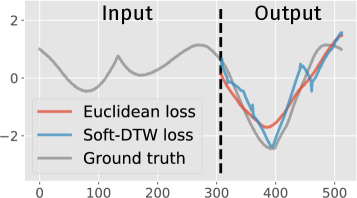
Figure 1: Given the first part of a time series, we trained two multi-layer perceptron (MLP) to predict the entire second part. Using the ShapesAll dataset, we used a Euclidean loss for the first MLP and the soft-DTW loss proposed in this paper for the second one. We display above the prediction obtained for a given test instance with either of these two MLPs in addition to the ground truth. Oftentimes, we observe that the soft-DTW loss enables us to better predict sharp changes. More time series predictions are given in Appendix F.

The DTW geometry. Because it encodes efficiently a useful class of invariances, DTW has often been used in a discriminative framework (with a $k$-NN or SVM classifier) to predict a real or a class label output, and engineered to run faster in that context (Yi et al., 1998). Recent works by Petitjean et al. (2011); Petitjean & Gançarski (2012) have, however, shown that DTW can be used for more innovative tasks, such as time series averaging using the DTW discrepancy (see Schultz & Jain 2017 for a gentle introduction to these ideas). More generally, the idea of synthetising time series centroids can be regarded as a first attempt to output entire time series using DTW as a fitting loss. From a computational perspective, these approaches are, however, hampered by the fact that DTW is not differentiable and unstable when used in an optimization pipeline.

Soft-DTW. In parallel to these developments, several authors have considered smoothed modifications of Bellman’s recursion to define smoothed DP distances (Bahl & Jelinek, 1975; Ristad & Yianilos, 1998) or kernels (Saigo et al., 2004; Cuturi et al., 2007). When applied to the DTW discrepancy, that regularization results in a soft-DTW score, which considers the soft-minimum of the distribution of all costs spanned by all possible alignments between two time series. Despite considering all alignments and not just the optimal one, soft-DTW can be computed with a minor modification of Bellman’s recursion, in which all $(\min,+)$ operations are replaced with $(+,\times)$. As a result, both DTW and soft-DTW have quadratic in time & linear in space complexity with respect to the sequences’ lengths. Because soft-DTW can be used with kernel machines, one typically observes an increase in performance when using soft-DTW over DTW (Cuturi, 2011) for classification.

Our contributions. We explore in this paper another important benefit of smoothing DTW: unlike the original DTW discrepancy, soft-DTW is differentiable in all of its arguments. We show that the gradients of soft-DTW w.r.t to all of its variables can be computed as a by-product of the computation of the discrepancy itself, with an added quadratic storage cost. We use this fact to propose an alternative approach to the DBA (DTW Barycenter Averaging) clustering algorithm of (Petitjean et al., 2011), and observe that our smoothed approach significantly outperforms known baselines for that task. More generally, we propose to use soft-DTW as a fitting term to compare the output of a machine synthesizing a time series segment with a ground truth observation, in the same way that, for instance, a regularized Wasserstein distance was used to compute barycenters (Cuturi & Doucet, 2014), and later to fit discriminators that output histograms (Zhang et al., 2015; Rolet et al., 2016). When paired with a flexible learning architecture such as a neural network, soft-DTW allows for a differentiable end-to-end approach to design predictive and generative models for time series, as illustrated in Figure 1. Source code is available at https://github.com/mblondel/soft-dtw.

Structure. After providing background material, we show in §2 how soft-DTW can be differentiated w.r.t the locations of two time series. We follow in §3 by illustrating how these results can be directly used for tasks that require to output time series: averaging, clustering and prediction of time series. We close this paper with experimental results in §4 that showcase each of these potential applications.

Notations. We consider in what follows multivariate discrete time series of varying length taking values in $\Omega\subset\mathbb{R}^{p}$. A time series can be thus represented as a matrix of $p$ lines and varying number of columns. We consider a differentiable substitution-cost function $\delta:\mathbb{R}^{p}\times\mathbb{R}^{p}\rightarrow\mathbb{R}_{+}$ which will be, in most cases, the quadratic Euclidean distance between two vectors. For an integer $n$ we write $\llbracket n\rrbracket$ for the set $\{1,\dots,n\}$ of integers. Given two series’ lengths $n$ and $m$, we write $\mathcal{A}_{n,m}\subset\{0,1\}^{n\times m}$ for the set of (binary) alignment matrices, that is paths on a $n\times m$ matrix that connect the upper-left $(1,1)$ matrix entry to the lower-right $(n,m)$ one using only $\downarrow,\rightarrow,\searrow$ moves. The cardinal of $\mathcal{A}_{n,m}$ is known as the $\text{delannoy}(n-1,m-1)$ number; that number grows exponentially with $m$ and $n$.

2 The DTW and soft-DTW loss functions

We propose in this section a unified formulation for the original DTW discrepancy (Sakoe & Chiba, 1978) and the Global Alignment kernel (GAK) (Cuturi et al., 2007), which can be both used to compare two time series $\mathbf{x}=(x_{1},\dots,x_{n})\in\mathbb{R}^{p\times n}$ and $\mathbf{y}=(y_{1},\dots,y_{m})\in\mathbb{R}^{p\times m}$.

2.1 Alignment costs: optimality and sum

Given the cost matrix $\Delta(\mathbf{x},\mathbf{y})\coloneqq\begin{bmatrix}\delta(x_{i},y_{j})\end{bmatrix}_{ij}\in\mathbb{R}^{n\times m}$, the inner product $\langle A,\Delta(\mathbf{x},\mathbf{y})\,\rangle$ of that matrix with an alignment matrix $A$ in $\mathcal{A}_{n,m}$ gives the score of $A$, as illustrated in Figure 2. Both DTW and GAK consider the costs of all possible alignment matrices, yet do so differently:

$$\text{DTW}(\mathbf{x},\mathbf{y}) \coloneqq\min_{A\in\mathcal{A}_{n,m}}\langle A,\Delta(\mathbf{x},\mathbf{y})\,\rangle,$$ (1)

$$k_{\text{GA}}^{\gamma}(\mathbf{x},\mathbf{y}) \coloneqq\sum_{A\in\mathcal{A}_{n,m}}e^{-\langle A,\Delta(\mathbf{x},\mathbf{y})\,\rangle/\gamma}.$$

DP Recursion. Sakoe & Chiba (1978) showed that the Bellman equation (1952) can be used to compute DTW. That recursion, which appears in line 5 of Algorithm 1 (disregarding for now the exponent $\gamma$), only involves $(\min,+)$ operations. When considering kernel $k_{\text{GA}}^{\gamma}$ and, instead, its integration over all alignments (see e.g. Lasserre 2009), Cuturi et al. (2007, Theorem 2) and the highly related formulation of Saigo et al. (2004, p.1685) use an old algorithmic appraoch (Bahl & Jelinek, 1975) which consists in (i) replacing all costs by their neg-exponential; (ii) replace $(\min,+)$ operations with $(+,\times)$ operations. These two recursions can be in fact unified with the use of a soft-minimum operator, which we present below.

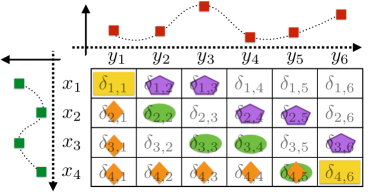
Figure 2: Three alignment matrices (orange, green, purple, in addition to the top-left and bottom-right entries) between two time series of length 4 and 6. The cost of an alignment is equal to the sum of entries visited along the path. DTW only considers the optimal alignment (here depicted in purple pentagons), whereas soft-DTW considers all $\text{delannoy}(n-1,m-1)$ possible alignment matrices.

Unified algorithm Both formulas in Eq. (1) can be computed with a single algorithm. That formulation is new to our knowledge. Consider the following generalized $\min$ operator, with a smoothing parameter $\gamma\geq 0$:

$$\operatorname{\operatorname{min}^{\gamma}}\{a_{1},\dots,a_{n}\}\coloneqq\begin{cases}\min_{i\leq n}a_{i},&\gamma=0,\\ -\gamma\log\sum_{i=1}^{n}e^{-a_{i}/\gamma},&\gamma>0.\end{cases}$$

With that operator, we can define $\gamma$-soft-DTW:

$$\boxed{\operatorname{\mathbf{dtw}_{\gamma}}(\mathbf{x},\mathbf{y})\coloneqq\operatorname{\operatorname{min}^{\gamma}}\{\langle A,\Delta(\mathbf{x},\mathbf{y})\,\rangle,A\in\mathcal{A}_{n,m}\}.}$$ (2)

The original DTW score is recovered by setting $\gamma$ to $0$. When $\gamma>0$, we recover $\operatorname{\mathbf{dtw}_{\gamma}}=-\gamma\log k_{\text{GA}}^{\gamma}$. Most importantly, and in either case, $\operatorname{\mathbf{dtw}_{\gamma}}$ can be computed using Algorithm 1, which requires $(nm)$ operations and $(nm)$ storage cost as well . That cost can be reduced to $2n$ with a more careful implementation if one only seeks to compute $\operatorname{\mathbf{dtw}_{\gamma}}(\mathbf{x},\mathbf{y})$, but the backward pass we consider next requires the entire matrix $R$ of intermediary alignment costs. Note that, to ensure numerical stability, the operator $\operatorname{\operatorname{min}^{\gamma}}$ must be computed using the usual log-sum-exp stabilization trick, namely that $\log\sum_{i}e^{z_{i}}=(\max_{j}z_{j})+\log\sum_{i}e^{z_{i}-\max_{j}z_{j}}.$

Algorithm 1 Forward recursion to compute $\operatorname{\mathbf{dtw}_{\gamma}}(\mathbf{x},\mathbf{y})$ and intermediate alignment costs

1:Inputs: $\mathbf{x,y}$, smoothing $\gamma\geq 0$, distance function $\delta$

2:$r_{0,0}=0;r_{i,0}=r_{0,j}=\infty;i\in\llbracket n\rrbracket,j\in\llbracket m\rrbracket$

3:for $j=1,\dots,m$ do

4:     for $i=1,\dots,n$ do

5:         $\!\!\!\!\!\!r_{i,j}=\delta(x_{i},y_{j})+\operatorname{\operatorname{min}^{\gamma}}\{r_{i-1,j-1},r_{i-1,j},r_{i,j-1}\}$

6:     end for

7:end for

8:Output: $(r_{n,m},R)$

2.2 Differentiation of soft-DTW

A small variation in the input $\mathbf{x}$ causes a small change in $\operatorname{\mathbf{dtw}_{0}}(\mathbf{x},\mathbf{y})$ or $\operatorname{\mathbf{dtw}_{\gamma}}(\mathbf{x},\mathbf{y})$. When considering $\operatorname{\mathbf{dtw}_{0}}$, that change can be efficiently monitored only when the optimal alignment matrix $A^{\star}$ that arises when computing $\operatorname{\mathbf{dtw}_{0}}(\mathbf{x},\mathbf{y})$ in Eq. (1) is unique. As the minimum over a finite set of linear functions of $\Delta$, $\operatorname{\mathbf{dtw}_{0}}$ is therefore locally differentiable w.r.t. the cost matrix $\Delta$, with gradient $A^{\star}$, a fact that has been exploited in all algorithms designed to average time series under the DTW metric (Petitjean et al., 2011; Schultz & Jain, 2017). To recover the gradient of $\operatorname{\mathbf{dtw}_{0}}(\mathbf{x},\mathbf{y})$ w.r.t. $\mathbf{x}$, we only need to apply the chain rule, thanks to the differentiability of the cost function:

$$\nabla_{\mathbf{x}}{\operatorname{\mathbf{dtw}_{0}}}(\mathbf{x},\mathbf{y})=\left(\frac{\partial\Delta(\mathbf{x},\mathbf{y})}{\partial\mathbf{x}}\right)^{T}A^{\star},$$ (3)

where $\partial\Delta(\mathbf{x},\mathbf{y})/\partial\mathbf{x}$ is the Jacobian of $\Delta$ w.r.t. $\mathbf{x}$, a linear map from $\mathbb{R}^{p\times n}$ to $\mathbb{R}^{n\times m}$. When $\delta$ is the squared Euclidean distance, the transpose of that Jacobian applied to a matrix $B\in\mathbb{R}^{n\times m}$ is ($\circ$ being the elementwise product):

$$(\partial\Delta(\mathbf{x},\mathbf{y})/\partial\mathbf{x})^{T}B=2\left((\mathbf{1}_{p}\mathbf{1}_{m}^{T}B^{T})\circ\mathbf{x}-\mathbf{y}B^{T}\right).$$

With continuous data, $A^{\star}$ is almost always likely to be unique, and therefore the gradient in Eq. (3) will be defined almost everywhere. However, that gradient, when it exists, will be discontinuous around those values $\mathbf{x}$ where a small change in $\mathbf{x}$ causes a change in $A^{\star}$, which is likely to hamper the performance of gradient descent methods.

The case $\gamma>0$.

An immediate advantage of soft-DTW is that it can be explicitly differentiated, a fact that was also noticed by  Saigo et al. (2006) in the related case of edit distances. When $\gamma>0$, the gradient of Eq. (1) is obtained via the chain rule,

$$\nabla_{\mathbf{x}}\operatorname{\mathbf{dtw}_{\gamma}}(\mathbf{x},\mathbf{y})=\left(\frac{\partial\Delta(\mathbf{x},\mathbf{y})}{\partial\mathbf{x}}\right)^{T}\mathbb{E}_{\gamma}[A],$$ (4)

$$\text{where}\quad\mathbb{E}_{\gamma}[A]\coloneqq\frac{1}{k_{\text{GA}}^{\gamma}(\mathbf{x},\mathbf{y})}\sum_{A\in\mathcal{A}_{n,m}}e^{-\langle A,\Delta(\mathbf{x},\mathbf{y})/\gamma\,\rangle}A,$$

is the average alignment matrix $A$ under the Gibbs distribution $p_{\gamma}\propto e^{-\langle A,\Delta(\mathbf{x},\mathbf{y})\,\rangle/\gamma}$ defined on all alignments in $\mathcal{A}_{n,m}$. The kernel $k_{\text{GA}}^{\gamma}(\mathbf{x},\mathbf{y})$ can thus be interpreted as the normalization constant of $p_{\gamma}$. Of course, since $\mathcal{A}_{n,m}$ has exponential size in $n$ and $m$, a naive summation is not tractable. Although a Bellman recursion to compute that average alignment matrix $\mathbb{E}_{\gamma}[A]$ exists (see Appendix A) that computation has quartic ($n^{2}m^{2}$) complexity. Note that this stands in stark contrast to the quadratic complexity obtained by Saigo et al. (2006) for edit-distances, which is due to the fact the sequences they consider can only take values in a finite alphabet. To compute the gradient of soft-DTW, we propose instead an algorithm that manages to remain quadratic ($nm$) in terms of complexity. The key to achieve this reduction is to apply the chain rule in reverse order of Bellman’s recursion given in Algorithm 1, namely backpropagate. A similar idea was recently used to compute the gradient of ANOVA kernels in (Blondel et al., 2016).

2.3 Algorithmic differentiation

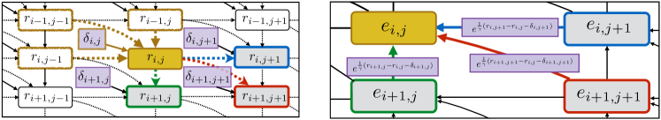
Figure 3: Sketch of the computational graph for soft-DTW, in the forward pass used to compute $\operatorname{\mathbf{dtw}_{\gamma}}$ (left) and backward pass used to compute its gradient $\nabla_{\mathbf{x}}\operatorname{\mathbf{dtw}_{\gamma}}$ (right). In both diagrams, purple shaded cells stand for data values available before the recursion starts, namely cost values (left) and multipliers computed using forward pass results (right). In the left diagram, the forward computation of $r_{i,j}$ as a function of its predecessors and $\delta_{i,j}$ is summarized with arrows. Dotted lines indicate a $\operatorname{\operatorname{min}^{\gamma}}$ operation, solid lines an addition. From the perspective of the final term $r_{n,m}$, which stores $\operatorname{\mathbf{dtw}_{\gamma}}(\mathbf{x},\mathbf{y})$ at the lower right corner (not shown) of the computational graph, a change in $r_{i,j}$ only impacts $r_{n,m}$ through changes that $r_{i,j}$ causes to $r_{i+1,j}$, $r_{i,j+1}$ and $r_{i+1,j+1}$. These changes can be tracked using Eq. (7,8) and appear in lines 9-11 in Algorithm 2 as variables $a,b,c$, as well as in the purple shaded boxes in the backward pass (right) which represents the recursion of line 12 in Algorithm 2.

Differentiating algorithmically $\operatorname{\mathbf{dtw}_{\gamma}}(\mathbf{x},\mathbf{y})$ requires doing first a forward pass of Bellman’s equation to store all intermediary computations and recover $R=[r_{i,j}]$ when running Algorithm 1. The value of $\operatorname{\mathbf{dtw}_{\gamma}}(\mathbf{x},\mathbf{y})$—stored in $r_{n,m}$ at the end of the forward recursion—is then impacted by a change in $r_{i,j}$ exclusively through the terms in which $r_{i,j}$ plays a role, namely the triplet of terms $r_{i+1,j},r_{i,j+1},r_{i+1,j+1}$. A straightforward application of the chain rule then gives

$$\!\!\underbrace{\tfrac{\partial r_{n,m}}{\partial r_{i,j}}}_{e_{i,j}}\!\!=\underbrace{\tfrac{\partial r_{n,m}}{\partial r_{i+1,j}}}_{e_{i+1,j}}\!\boldsymbol{{\color[rgb]{0.05,0.50,0.15}\tfrac{\partial r_{i+1,j}}{\partial r_{i,j}}}}+\underbrace{\tfrac{\partial r_{n,m}}{\partial r_{i,j+1}}}_{e_{i,j+1}}\!\boldsymbol{{\color[rgb]{0,0,1}\tfrac{\partial r_{i,j+1}}{\partial r_{i,j}}}}+\underbrace{\tfrac{\partial r_{n,m}}{\partial r_{i+1,j+1}}}_{e_{i+1,j+1}}\!\boldsymbol{{\color[rgb]{1,0,0}\tfrac{\partial r_{i+1,j+1}}{\partial r_{i,j}}}},$$ (5)

in which we have defined the notation of the main object of interest of the backward recursion: $e_{i,j}\coloneqq\tfrac{\partial r_{n,m}}{\partial r_{i,j}}$. The Bellman recursion evaluated at $(i+1,j)$ as shown in line 5 of Algorithm 1 (here $\delta_{i+1,j}$ is $\delta(x_{i+1},y_{j})$) yields :

$$r_{i+1,j}=\delta_{i+1,j}+\operatorname{\operatorname{min}^{\gamma}}\{r_{i,j-1},r_{i,j},r_{i+1,j-1}\},$$ (6)

which, when differentiated w.r.t $r_{i,j}$ yields the ratio:

$$\boldsymbol{{\color[rgb]{0.05,0.50,0.15}\tfrac{\partial r_{i+1,j}}{\partial r_{i,j}}}}=e^{-r_{i,j}/\gamma}/\left(e^{-r_{i,j-1}/\gamma}+e^{-r_{i,j}/\gamma}+e^{-r_{i+1,j-1}/\gamma}\right).$$

The logarithm of that derivative can be conveniently cast using evaluations of $\operatorname{\operatorname{min}^{\gamma}}$ computed in the forward loop:

$$\gamma\log\boldsymbol{{\color[rgb]{0.05,0.50,0.15}\tfrac{\partial r_{i+1,j}}{\partial r_{i,j}}}} =\operatorname{\operatorname{min}^{\gamma}}\{r_{i,j-1},r_{i,j},r_{i+1,j-1}\}-r_{i,j}$$ (7)

$$=r_{i+1,j}-\delta_{i+1,j}-r_{i,j}.$$

Similarly, the following relationships can also be obtained:

$$\gamma\log\boldsymbol{{\color[rgb]{0,0,1}\tfrac{\partial r_{i,j+1}}{\partial r_{i,j}}}} =r_{i,j+1}-r_{i,j}-\delta_{i,j+1},$$ (8)

$$\gamma\log\boldsymbol{{\color[rgb]{1,0,0}\tfrac{\partial r_{i+1,j+1}}{\partial r_{i,j}}}} =r_{i+1,j+1}-r_{i,j}-\delta_{i+1,j+1}.$$

We have therefore obtained a backward recursion to compute the entire matrix $E=[e_{i,j}]$, starting from $e_{n,m}=\tfrac{\partial r_{n,m}}{\partial r_{n,m}}=1$ down to $e_{1,1}$. To obtain $\nabla_{\mathbf{x}}\operatorname{\mathbf{dtw}_{\gamma}}(\mathbf{x},\mathbf{y})$, notice that the derivatives w.r.t. the entries of the cost matrix $\Delta$ can be computed by $\tfrac{\partial r_{n,m}}{\partial\delta_{i,j}}=\tfrac{\partial r_{n,m}}{\partial r_{i,j}}\tfrac{\partial r_{i,j}}{\partial\delta_{i,j}}=e_{i,j}\cdot 1=e_{i,j},$ and therefore we have that

$$\nabla_{\mathbf{x}}\operatorname{\mathbf{dtw}_{\gamma}}(\mathbf{x},\mathbf{y})=\left(\frac{\partial\Delta(\mathbf{x},\mathbf{y})}{\partial\mathbf{x}}\right)^{T}E,$$

where $E$ is exactly the average alignment $\mathbb{E}_{\gamma}[A]$ in Eq. (4). These computations are summarized in Algorithm 2, which, once $\Delta$ has been computed, has complexity $nm$ in time and space. Because $\operatorname{\operatorname{min}^{\gamma}}$ has a $1/\gamma$-Lipschitz continuous gradient, the gradient of $\operatorname{\mathbf{dtw}_{\gamma}}$ is $2/\gamma$-Lipschitz continuous when $\delta$ is the squared Euclidean distance.

Algorithm 2 Backward recursion to compute $\nabla_{\mathbf{x}}\operatorname{\mathbf{dtw}_{\gamma}}(\mathbf{x},\mathbf{y})$

1:Inputs: $\mathbf{x},\mathbf{y}$, smoothing $\gamma\geq 0$, distance function $\delta$

2:$(\cdot,R)=\operatorname{\mathbf{dtw}_{\gamma}}(\mathbf{x},\mathbf{y})$, $\Delta=[\delta(x_{i},y_{j})]_{i,j}$

3:$\delta_{i,m+1}=\delta_{n+1,j}=0,i\in\llbracket n\rrbracket,j\in\llbracket m\rrbracket$

4:$e_{i,m+1}=e_{n+1,j}=0,i\in\llbracket n\rrbracket,j\in\llbracket m\rrbracket$

5:$r_{i,m+1}=r_{n+1,j}=-\infty,i\in\llbracket n\rrbracket,j\in\llbracket m\rrbracket$

6:$\delta_{n+1,m+1}=0,e_{n+1,m+1}=1,r_{n+1,m+1}=r_{n,m}$

7:for $j=m,\dots,1$ do

8:     for $i=n,\dots,1$ do

9:         $\!\!\!\!\!\!a=\exp\frac{1}{\gamma}(r_{i+1,j}-r_{i,j}-\delta_{i+1,j})$

10:         $\!\!\!\!\!\!b=\exp\frac{1}{\gamma}(r_{i,j+1}-r_{i,j}-\delta_{i,j+1})$

11:         $\!\!\!\!\!\!c=\exp\frac{1}{\gamma}(r_{i+1,j+1}-r_{i,j}-\delta_{i+1,j+1})$

12:         $\!\!\!\!\!\!e_{i,j}=e_{i+1,j}\cdot a+e_{i,j+1}\cdot b+e_{i+1,j+1}\cdot c$

13:     end for

14:end for

15:Output: $\nabla_{\mathbf{x}}\operatorname{\mathbf{dtw}_{\gamma}}(\mathbf{x},\mathbf{y})=\left(\frac{\partial\Delta(\mathbf{x},\mathbf{y})}{\partial\mathbf{x}}\right)^{T}E$

3 Learning with the soft-DTW loss

3.1 Averaging with the soft-DTW geometry

We study in this section a direct application of Algorithm 2 to the problem of computing Fréchet means (1948) of time series with respect to the $\operatorname{\mathbf{dtw}_{\gamma}}$ discrepancy. Given a family of $N$ times series $\mathbf{y}_{1},\dots,\mathbf{y}_{N}$, namely $N$ matrices of $p$ lines and varying number of columns, $m_{1},\dots,m_{N}$, we are interested in defining a single barycenter time series $\mathbf{x}$ for that family under a set of normalized weights $\lambda_{1},\dots,\lambda_{N}\in\mathbb{R}_{+}$ such that $\sum_{i=1}^{N}\lambda_{i}=1$. Our goal is thus to solve approximately the following problem, in which we have assumed that $\mathbf{x}$ has fixed length $n$:

$$\min_{\mathbf{x}\in\mathbb{R}^{p\times n}}\sum_{i=1}^{N}\frac{\lambda_{i}}{m_{i}}\operatorname{\mathbf{dtw}_{\gamma}}(\mathbf{x},\mathbf{y}_{i}).$$ (9)

Note that each $\operatorname{\mathbf{dtw}_{\gamma}}(\mathbf{x},\mathbf{y}_{i})$ term is divided by $m_{i}$, the length of $\mathbf{y}_{i}$. Indeed, since $\operatorname{\mathbf{dtw}_{0}}$ is an increasing (roughly linearly) function of each of the input lengths $n$ and $m_{i}$, we follow the convention of normalizing in practice each discrepancy by $n\times m_{i}$. Since the length $n$ of $\mathbf{x}$ is here fixed across all evaluations, we do not need to divide the objective of Eq. (9) by $n$. Averaging under the soft-DTW geometry results in substantially different results than those that can be obtained with the Euclidean geometry (which can only be used in the case where all lengths $n=m_{1}=\dots=m_{N}$ are equal), as can be seen in the intuitive interpolations we obtain between two time series shown in Figure 4.

Non-convexity of $\operatorname{\mathbf{dtw}_{\gamma}}$. A natural question that arises from Eq. (9) is whether that objective is convex or not. The answer is negative, in a way that echoes the non-convexity of the $k$-means objective as a function of cluster centroids locations. Indeed, for any alignment matrix $A$ of suitable size, each map $\mathbf{x}\mapsto\langle A,\Delta(\mathbf{x},\mathbf{y})\,\rangle$ shares the same convexity/concavity property that $\delta$ may have. However, both $\min$ and $\operatorname{\operatorname{min}^{\gamma}}$ can only preserve the concavity of elementary functions (Boyd & Vandenberghe, 2004, pp.72-74). Therefore $\operatorname{\mathbf{dtw}_{\gamma}}$ will only be concave if $\delta$ is concave, or become instead a (non-convex) (soft) minimum of convex functions if $\delta$ is convex. When $\delta$ is a squared-Euclidean distance, $\operatorname{\mathbf{dtw}_{0}}$ is a piecewise quadratic function of $\mathbf{x}$, as is also the case with the $k$-means energy (see for instance Figure 2 in Schultz & Jain 2017). Since this is the setting we consider here, all of the computations involving barycenters should be taken with a grain of salt, since we have no way of ensuring optimality when approximating Eq. (9).

Smoothing helps optimizing $\operatorname{\mathbf{dtw}_{\gamma}}$. Smoothing can be regarded, however, as a way to “convexify” $\operatorname{\mathbf{dtw}_{\gamma}}$. Indeed, notice that $\operatorname{\mathbf{dtw}_{\gamma}}$ converges to the sum of all costs as $\gamma\rightarrow\infty$. Therefore, if $\delta$ is convex, $\operatorname{\mathbf{dtw}_{\gamma}}$ will gradually become convex as $\gamma$ grows. For smaller values of $\gamma$, one can intuitively foresee that using $\operatorname{\operatorname{min}^{\gamma}}$ instead of a minimum will smooth out local minima and therefore provide a better (although slightly different from $\operatorname{\mathbf{dtw}_{0}}$) optimization landscape. We believe this is why our approach recovers better results, even when measured in the original $\operatorname{\mathbf{dtw}_{0}}$ discrepancy, than subgradient or alternating minimization approaches such as DBA (Petitjean et al., 2011), which can, on the contrary, get more easily stuck in local minima. Evidence for this statement is presented in the experimental section.

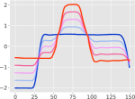
(a) Euclidean loss

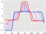
(b) Soft-DTW loss ($\gamma=1$)

Figure 4: Interpolation between two time series (red and blue) on the Gun Point dataset. We computed the barycenter by solving Eq. (9) with $(\lambda_{1},\lambda_{2})$ set to (0.25, 0.75), (0.5, 0.5) and (0.75, 0.25). The soft-DTW geometry leads to visibly different interpolations.

3.2 Clustering with the soft-DTW geometry

The (approximate) computation of $\operatorname{\mathbf{dtw}_{\gamma}}$ barycenters can be seen as a first step towards the task of clustering time series under the $\operatorname{\mathbf{dtw}_{\gamma}}$ discrepancy. Indeed, one can naturally formulate that problem as that of finding centroids $\mathbf{x}_{1},\dots,\mathbf{x}_{k}$ that minimize the following energy:

$$\min_{\mathbf{x}_{1},\dots,\mathbf{x}_{k}\in\mathbb{R}^{p\times n}}\sum_{i=1}^{N}\frac{1}{m_{i}}\min_{j\in[[k]]}\operatorname{\mathbf{dtw}_{\gamma}}(\mathbf{x}_{j},\mathbf{y}_{i}).$$ (10)

To solve that problem one can resort to a direct generalization of Lloyd’s algorithm (1982) in which each centering step and each clustering allocation step is done according to the $\operatorname{\mathbf{dtw}_{\gamma}}$ discrepancy.

3.3 Learning prototypes for time series classification

One of the de-facto baselines for learning to classify time series is the $k$ nearest neighbors ($k$-NN) algorithm, combined with DTW as discrepancy measure between time series. However, $k$-NN has two main drawbacks. First, the time series used for training must be stored, leading to potentially high storage cost. Second, in order to compute predictions on new time series, the DTW discrepancy must be computed with all training time series, leading to high computational cost. Both of these drawbacks can be addressed by the nearest centroid classifier (Hastie et al., 2001, p.670), (Tibshirani et al., 2002). This method chooses the class whose barycenter (centroid) is closest to the time series to classify. Although very simple, this method was shown to be competitive with $k$-NN, while requiring much lower computational cost at prediction time (Petitjean et al., 2014). Soft-DTW can naturally be used in a nearest centroid classifier, in order to compute the barycenter of each class at train time, and to compute the discrepancy between barycenters and time series, at prediction time.

3.4 Multistep-ahead prediction

Soft-DTW is ideally suited as a loss function for any task that requires time series outputs. As an example of such a task, we consider the problem of, given the first $1,\dots,t$ observations of a time series, predicting the remaining $(t+1),\dots,n$ observations. Let $\mathbf{x}^{t,t^{\prime}}\in\mathbb{R}^{p\times(t^{\prime}-t+1)}$ be the submatrix of $\mathbf{x}\in\mathbb{R}^{p\times n}$ of all columns with indices between $t$ and $t^{\prime}$, where $1\leq t<t^{\prime}<n$. Learning to predict the segment of a time series can be cast as the problem

$$\min_{\theta\in\Theta}\sum_{i=1}^{N}\operatorname{\mathbf{dtw}_{\gamma}}\left(f_{\theta}(\mathbf{x}_{i}^{1,t}),\mathbf{x}_{i}^{t+1,n}\right),$$ (11)

where $\{f_{\theta}\}$ is a set of parameterized function that take as input a time series and outputs a time series. Natural choices would be multi-layer perceptrons or recurrent neural networks (RNN), which have been historically trained with a Euclidean loss (Parlos et al., 2000, Eq.5).

4 Experimental results

Throughout this section, we use the UCR (University of California, Riverside) time series classification archive (Chen et al., 2015). We use a subset containing 79 datasets encompassing a wide variety of fields (astronomy, geology, medical imaging) and lengths. Datasets include class information (up to 60 classes) for each time series and are split into train and test sets. Due to the large number of datasets in the UCR archive, we choose to report only a summary of our results in the main manuscript. Detailed results are included in the appendices for interested readers.

4.1 Averaging experiments

In this section, we compare the soft-DTW barycenter approach presented in §3.1 to DBA (Petitjean et al., 2011) and a simple batch subgradient method.

Experimental setup. For each dataset, we choose a class at random, pick 10 time series in that class and compute their barycenter. For quantitative results below, we repeat this procedure 10 times and report the averaged results. For each method, we set the maximum number of iterations to 100. To minimize the proposed soft-DTW barycenter objective, Eq. (9), we use L-BFGS.

Table 1: Percentage of the datasets on which the proposed soft-DTW barycenter is achieving lower DTW loss (Equation (9) with $\gamma=0$) than competing methods.

	Random initialization	Euclidean mean initialization
Comparison with DBA
$\gamma=1$	40.51%	3.80%
$\gamma=0.1$	93.67%	46.83%
$\gamma=0.01$	100%	79.75%
$\gamma=0.001$	97.47%	89.87%
Comparison with subgradient method
$\gamma=1$	96.20%	35.44%
$\gamma=0.1$	97.47%	72.15%
$\gamma=0.01$	97.47%	92.41%
$\gamma=0.001$	97.47%	97.47%

Qualitative results. We first visualize the barycenters obtained by soft-DTW when $\gamma=1$ and $\gamma=0.01$, by DBA and by the subgradient method. Figure 5 shows barycenters obtained using random initialization on the ECG200 dataset. More results with both random and Euclidean mean initialization are given in Appendix B and C.

We observe that both DBA or soft-DTW with low smoothing parameter $\gamma$ yield barycenters that are spurious. On the other hand, a descent on the soft-DTW loss with sufficiently high $\gamma$ converges to a reasonable solution. For example, as indicated in Figure 5 with DTW or soft-DTW ($\gamma=0.01$), the small kink around $x=15$ is not representative of any of the time series in the dataset. However, with soft-DTW ($\gamma=1$), the barycenter closely matches the time series. This suggests that DTW or soft-DTW with too low $\gamma$ can get stuck in bad local minima.

When using Euclidean mean initialization (only possible if time series have the same length), DTW or soft-DTW with low $\gamma$ often yield barycenters that better match the shape of the time series. However, they tend to overfit: they absorb the idiosyncrasies of the data. In contrast, soft-DTW is able to learn barycenters that are much smoother.

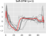
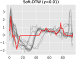
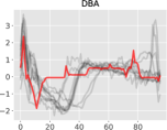
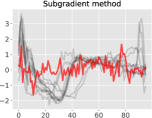
Figure 5: Comparison between our proposed soft barycenter and the barycenter obtained by DBA and the subgradient method, on the ECG200 dataset. When DTW is insufficiently smoothed, barycenters often get stuck in a bad local minimum that does not correctly match the time series.

Quantitative results. Table 1 summarizes the percentage of datasets on which the proposed soft-DTW barycenter achieves lower DTW loss when varying the smoothing parameter $\gamma$. The actual loss values achieved by different methods are indicated in Appendix G and Appendix H.

As $\gamma$ decreases, soft-DTW achieves a lower DTW loss than other methods on almost all datasets. This confirms our claim that the smoothness of soft-DTW leads to an objective that is better behaved and more amenable to optimization by gradient-descent methods.

4.2 $k$-means clustering experiments

We consider in this section the same computational tools used in §4.1 above, but use them to cluster time series.

Experimental setup. For all datasets, the number of clusters $k$ is equal to the number of classes available in the dataset. Lloyd’s algorithm alternates between a centering step (barycenter computation) and an assignment step. We set the maximum number of outer iterations to $30$ and the maximum number of inner (barycenter) iterations to 100, as before. Again, for soft-DTW, we use L-BFGS.

Qualitative results. Figure 6 shows the clusters obtained when runing Lloyd’s algorithm on the CBF dataset with soft-DTW ($\gamma=1$) and DBA, in the case of random initialization. More results are included in Appendix E. Clearly, DTW absorbs the tiny details in the data, while soft-DTW is able to learn much smoother barycenters.

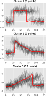
(a) Soft-DTW ($\gamma=1$)

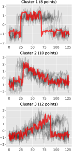
(b) DBA

Figure 6: Clusters obtained on the CBF dataset when plugging our proposed soft barycenter and that of DBA in Lloyd’s algorithm. DBA absorbs the idiosyncrasies of the data, while soft-DTW can learn much smoother barycenters.

Quantitative results. Table 2 summarizes the percentage of datasets on which soft-DTW barycenter achieves lower $k$-means loss under DTW, i.e. Eq. (10) with $\gamma=0$. The actual loss values achieved by all methods are indicated in Appendix I and Appendix J. The results confirm the same trend as for the barycenter experiments. Namely, as $\gamma$ decreases, soft-DTW is able to achieve lower loss than other methods on a large proportion of the datasets. Note that we have not run experiments with smaller values of $\gamma$ than 0.001, since $\mathbf{dtw}_{0.001}$ is very close to $\operatorname{\mathbf{dtw}_{0}}$ in practice.

Table 2: Percentage of the datasets on which the proposed soft-DTW based $k$-means is achieving lower DTW loss (Equation (10) with $\gamma=0$) than competing methods.

	Random initialization	Euclidean mean initialization
Comparison with DBA
$\gamma=1$	15.78%	29.31%
$\gamma=0.1$	24.56%	24.13%
$\gamma=0.01$	59.64%	55.17%
$\gamma=0.001$	77.19%	68.97%
Comparison with subgradient method
$\gamma=1$	42.10%	46.44%
$\gamma=0.1$	57.89%	50%
$\gamma=0.01$	76.43%	65.52%
$\gamma=0.001$	96.49%	84.48%

4.3 Time-series classification experiments

In this section, we investigate whether the smoothing in soft-DTW can act as a useful regularization and improve classification accuracy in the nearest centroid classifier.

Experimental setup. We use 50% of the data for training, 25% for validation and 25% for testing. We choose $\gamma$ from 15 log-spaced values between $10^{-3}$ and $10$.

Quantitative results. Each point in Figure 7 above the diagonal line represents a dataset for which using soft-DTW for barycenter computation rather than DBA improves the accuracy of the nearest centroid classifier. To summarize, we found that soft-DTW is working better or at least as well as DBA in 75% of the datasets.

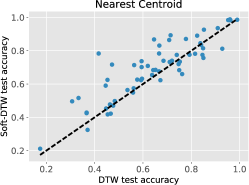
Figure 7: Each point above the diagonal represents a dataset where using our soft-DTW barycenter rather than that of DBA improves the accuracy of the nearest nearest centroid classifier. This is the case for 75% of the datasets in the UCR archive.

4.4 Multistep-ahead prediction experiments

In this section, we present preliminary experiments for the task of multistep-ahead prediction, described in §3.4.

Experimental setup. We use the training and test sets pre-defined in the UCR archive. In both the training and test sets, we use the first 60% of the time series as input and the remaining 40% as output, ignoring class information. We then use the training set to learn a model that predicts the outputs from inputs and the test set to evaluate results with both Euclidean and DTW losses. In this experiment, we focus on a simple multi-layer perceptron (MLP) with one hidden layer and sigmoid activation. We also experimented with linear models and recurrent neural networks (RNNs) but they did not improve over a simple MLP.

Implementation details. Deep learning frameworks such as Theano, TensorFlow and Chainer allow the user to specify a custom backward pass for their function. Implementing such a backward pass, rather than resorting to automatic differentiation (autodiff), is particularly important in the case of soft-DTW: First, the autodiff in these frameworks is designed for vectorized operations, whereas the dynamic program used by the forward pass of Algorithm 1 is inherently element-wise; Second, as we explained in §2.2, our backward pass is able to re-use log-sum-exp computations from the forward pass, leading to both lower computational cost and better numerical stability. We implemented a custom backward pass in Chainer, which can then be used to plug soft-DTW as a loss function in any network architecture. To estimate the MLP’s parameters, we used Chainer’s implementation of Adam (Kingma & Ba, 2014).

Qualitative results. Visualizations of the predictions obtained under Euclidean and soft-DTW losses are given in Figure 1, as well as in Appendix F. We find that for simple one-dimensional time series, an MLP works very well, showing its ability to capture patterns in the training set. Although the predictions under Euclidean and soft-DTW losses often agree with each other, they can sometimes be visibly different. Predictions under soft-DTW loss can confidently predict abrupt and sharp changes since those have a low DTW cost as long as such a sharp change is present, under a small time shift, in the ground truth.

Quantitative results. A comparison summary of our MLP under Euclidean and soft-DTW losses over the UCR archive is given in Table 3. Detailed results are given in the appendix. Unsurprisingly, we achieve lower DTW loss when training with the soft-DTW loss, and lower Euclidean loss when training with the Euclidean loss. Because DTW is robust to several useful invariances, a small error in the soft-DTW sense could be a more judicious choice than an error in an Euclidean sense for many applications.

Table 3: Averaged rank obtained by a multi-layer perceptron (MLP) under Euclidean and soft-DTW losses. Euclidean initialization means that we initialize the MLP trained with soft-DTW loss by the solution of the MLP trained with Euclidean loss.

Training loss	Random initialization	Euclidean initialization
When evaluating with DTW loss
Euclidean	3.46	4.21
soft-DTW ($\gamma=1$)	3.55	3.96
soft-DTW ($\gamma=0.1$)	3.33	3.42
soft-DTW ($\gamma=0.01$)	2.79	2.12
soft-DTW ($\gamma=0.001$)	1.87	1.29
When evaluating with Euclidean loss
Euclidean	1.05	1.70
soft-DTW ($\gamma=1$)	2.41	2.99
soft-DTW ($\gamma=0.1$)	3.42	3.38
soft-DTW ($\gamma=0.01$)	4.13	3.64
soft-DTW ($\gamma=0.001$)	3.99	3.29

5 Conclusion

We propose in this paper to turn the popular DTW discrepancy between time series into a full-fledged loss function between ground truth time series and outputs from a learning machine. We have shown experimentally that, on the existing problem of computing barycenters and clusters for time series data, our computational approach is superior to existing baselines. We have shown promising results on the problem of multistep-ahead time series prediction, which could prove extremely useful in settings where a user’s actual loss function for time series is closer to the robust perspective given by DTW, than to the local parsing of the Euclidean distance.

Acknowledgements.

MC gratefully acknowledges the support of a chaire de l’IDEX Paris Saclay.

Appendix material

Appendix A Recursive forward computation of the average path matrix

The average alignment under Gibbs distribution $p_{\gamma}$ can be computed with the following forward recurrence, which mimics closely Bellman’s original recursion. For each $i\in\llbracket n\rrbracket,j\in\llbracket m\rrbracket$, define

$$E_{i+1,j+1}=\begin{bmatrix}e^{-\delta_{i+1,j+1}/\gamma}E_{i,j}&\mathbf{0}_{i}\\ \mathbf{0}_{j}^{T}&e^{-r_{i+1,j+1}/\gamma}\end{bmatrix}+\begin{bmatrix}\lx@intercol\hfil e^{-\delta_{i+1,j+1}/\gamma}E_{i,j+1}\hfil\lx@intercol\\ \mathbf{0}_{j}^{T}&e^{-r_{i+1,j+1}/\gamma}\end{bmatrix}+\begin{bmatrix}\hbox{\multirowsetup$e^{-\delta_{i+1,j+1}/\gamma}E_{i+1,j}$}&\mathbf{0}_{i}\\ &e^{-r_{ij}/\gamma}\end{bmatrix}$$

Here terms $r_{ij}$ are computed following the recursion in Algorithm 2. Border matrices are initialized to $0$, except for $E_{1,1}$ which is initialized to $[1]$. Upon completion, the average alignment matrix is stored in $E_{n,m}$.

The operation above consists in summing three matrices of size $(i+1,j+1)$. There are exactly $(nm)$ such updates. A careful implementation of this algorithm, that would only store two arrays of matrices, as Algorithm 1 only store two arrays of values, can be carried out in $nm\min(n,m)$ space but it would still require $(nm)^{2}$ operations.

Appendix B Barycenters obtained with random initialization

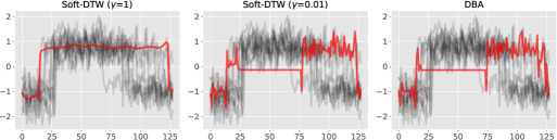
(a) CBF

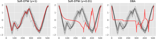
(b) Herring

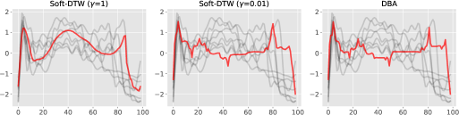
(c) Medical Images

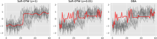
(d) Synthetic Control

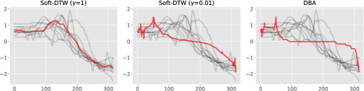
(e) Wave Gesture Library Y

Appendix C Barycenters obtained with Euclidean mean initialization

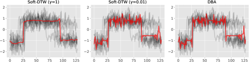
(a) CBF

(b) Herring

(c) Medical Images

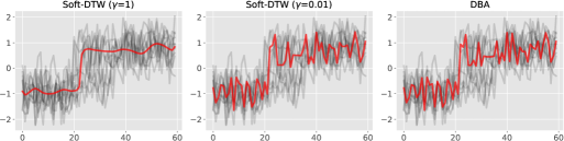
(d) Synthetic Control

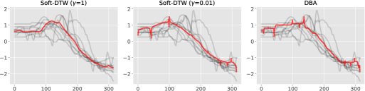
(e) Wave Gesture Library Y

Appendix D More interpolation results

Left: results obtained under Euclidean loss. Right: results obtained under soft-DTW ($\gamma=1$) loss.

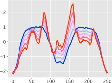
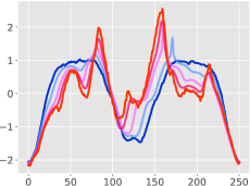
(a) ArrowHead

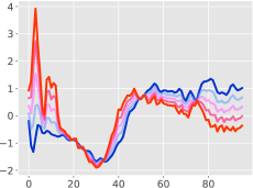
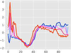
(b) ECG200

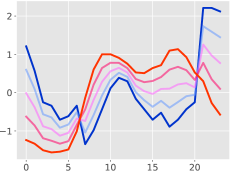
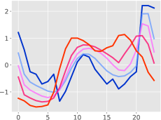
(c) ItalyPowerDemand

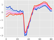
(d) TwoLeadECG

Appendix E Clusters obtained by $k$-means under DTW or soft-DTW geometry

CBF dataset

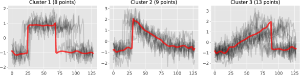
(a) Soft-DTW ($\gamma=1$, random initialization)

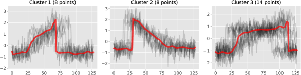
(b) Soft-DTW ($\gamma=1$, Euclidean mean initialization)

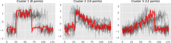
(c) DBA (random initialization)

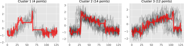
(d) DBA (Euclidean mean initialization)

ECG200 dataset

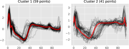
(a) Soft-DTW ($\gamma=1$, random initialization)

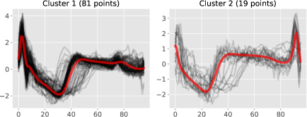
(b) Soft-DTW ($\gamma=1$, Euclidean mean initialization)

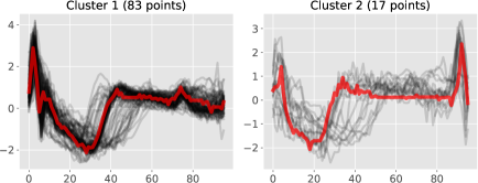
(c) DBA (random initialization)

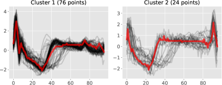
(d) DBA (Euclidean mean initialization)

Appendix F More visualizations of time-series prediction

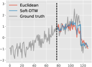
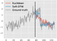
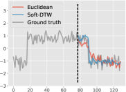
(a) CBF

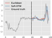
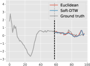
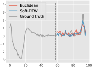
(b) ECG200

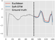
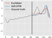
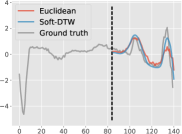
(c) ECG5000

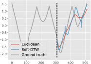
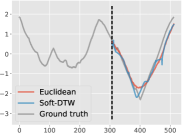
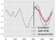
(d) ShapesAll

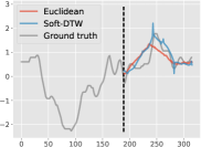
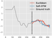
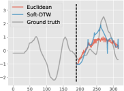
(e) uWaveGestureLibrary_Y

Appendix G Barycenters: DTW loss (Eq. 9 with $\gamma=0$) achieved with random init

Dataset	Soft-DTW $\gamma=1$	$\gamma=0.1$	$\gamma=0.01$	$\gamma=0.001$	Subgradient method	DBA	Euclidean mean
50words	5.000	2.785	2.513	2.721	44.399	4.554	25.388
Adiac	0.235	0.207	0.257	0.428	25.533	0.754	0.177
ArrowHead	2.390	1.598	1.487	1.664	36.125	2.512	2.743
Beef	10.471	6.541	6.200	6.238	88.100	7.780	25.347
BeetleFly	35.790	23.655	22.559	23.105	77.993	25.122	191.574
BirdChicken	23.300	12.542	11.164	11.954	45.777	12.820	92.061
CBF	21.098	11.949	12.564	12.667	30.281	14.836	28.236
Car	2.639	1.750	1.611	1.914	80.437	2.609	5.106
ChlorineConcentration	22.260	13.932	14.818	15.044	32.134	16.168	15.411
CinC_ECG_torso	118.872	80.248	76.536	76.812	262.221	90.663	761.238
Coffee	1.036	0.871	1.262	1.630	41.741	2.380	0.591
Computers	231.421	182.380	178.184	179.886	$\infty$	183.388	391.830
Cricket_X	41.514	29.290	28.424	28.851	70.128	28.955	104.699
Cricket_Y	51.858	30.321	30.337	31.041	70.989	33.098	107.712
Cricket_Z	43.458	30.264	28.668	29.373	68.382	32.182	128.129
DiatomSizeReduction	0.055	0.054	0.064	0.132	49.308	0.418	0.033
DistalPhalanxOutlineAgeGroup	1.380	1.074	1.407	1.509	11.539	1.761	0.981
DistalPhalanxOutlineCorrect	2.501	1.968	2.267	2.634	13.169	2.991	2.374
DistalPhalanxTW	1.148	0.906	1.015	1.159	10.957	1.228	0.867
ECG200	7.374	6.400	6.871	7.047	19.514	8.257	10.107
ECG5000	8.951	8.961	10.601	10.265	34.558	12.098	14.517
ECGFiveDays	9.816	9.019	9.364	9.407	17.898	9.837	23.975
Earthquakes	148.959	85.219	85.470	85.515	$\infty$	85.788	330.776
ElectricDevices	27.852	23.769	23.783	24.009	$\infty$	24.869	56.470
FISH	0.978	0.641	0.662	0.957	63.566	1.680	1.543
FaceAll	15.068	12.373	13.248	13.494	24.582	15.980	29.982
FaceFour	15.500	14.519	15.002	14.849	$\infty$	16.339	25.410
FacesUCR	15.033	13.077	13.405	14.174	30.621	14.796	27.026
FordA	56.936	45.492	46.170	46.038	96.087	49.723	218.482
FordB	59.117	47.812	47.058	47.642	102.279	50.262	250.595
Gun_Point	7.204	2.507	2.037	2.211	22.590	2.374	7.286
Ham	24.833	19.101	20.397	20.713	55.769	22.807	30.685
HandOutlines	3.400	2.690	2.814	28.759	353.235	3.422	7.838
Haptics	16.424	14.351	14.129	14.320	172.988	16.464	39.559
Herring	1.212	0.946	1.022	1.349	71.388	2.097	1.884
InlineSkate	83.107	29.672	22.819	N/A	N/A	N/A	N/A
ItalyPowerDemand	2.442	2.124	2.316	2.372	5.434	2.355	2.329
MedicalImages	6.934	5.809	5.980	6.089	22.777	6.252	10.911
MiddlePhalanxOutlineAgeGroup	0.858	0.753	1.305	1.375	11.474	1.605	0.624
MiddlePhalanxOutlineCorrect	0.832	0.714	0.985	1.030	11.643	1.678	0.611
MiddlePhalanxTW	0.755	0.581	0.963	1.206	10.684	1.274	0.447
MoteStrain	24.177	21.639	21.616	21.554	32.007	22.437	26.646
NonInvasiveFatalECG_Thorax1	6.671	3.324	4.738	5.031	59.162	6.378	3.568
NonInvasiveFatalECG_Thorax2	2.559	3.159	3.587	4.097	40339.200	6.494	2.864
OSULeaf	30.041	20.692	20.034	19.950	76.057	23.915	136.512
OliveOil	0.657	0.959	1.494	1.804	95.499	3.420	0.008
PhalangesOutlinesCorrect	1.383	1.114	1.405	1.516	11.070	1.743	1.210
Phoneme	99.205	72.412	73.666	73.767	157.124	78.664	138.157
Plane	1.079	0.849	1.220	1.629	20.328	2.111	1.209
ProximalPhalanxOutlineAgeGroup	0.618	0.511	0.691	0.878	10.437	1.177	0.322
ProximalPhalanxOutlineCorrect	0.749	0.654	0.833	0.882	10.767	1.111	0.615
ProximalPhalanxTW	0.653	0.536	0.672	0.778	10.377	1.133	0.462
RefrigerationDevices	159.745	146.601	140.634	141.200	$\infty$	148.931	363.732
ScreenType	156.442	123.746	121.432	122.247	$\infty$	132.748	334.379
ShapeletSim	236.039	123.605	125.657	126.062	154.480	130.428	283.458
ShapesAll	15.267	7.108	6.466	6.818	58.734	8.236	67.790
SmallKitchenAppliances	176.073	164.419	162.009	162.585	$\infty$	168.170	524.542
SonyAIBORobotSurface	5.735	4.916	5.425	5.337	$\infty$	5.813	5.430
SonyAIBORobotSurfaceII	11.994	11.048	11.278	11.405	6637415.793	11.481	13.783
StarLightCurves	22.342	11.757	7.934	7.654	102.255	11.600	47.353
Strawberry	1.392	1.191	1.477	1.627	28.696	2.347	1.300
SwedishLeaf	2.409	1.968	2.476	2.904	19.638	3.283	6.274
Symbols	0.845	0.488	0.439	0.460	$\infty$	0.828	4.953
ToeSegmentation1	35.904	27.461	26.554	26.988	63.040	29.838	129.858
ToeSegmentation2	34.177	24.476	23.003	23.194	$\infty$	24.944	170.222
Trace	2.686	1.453	0.870	1.031	43.017	2.233	26.037
TwoLeadECG	1.811	1.514	1.641	1.701	7.961	1.802	2.216
Two_Patterns	12.048	9.294	7.764	8.143	22.489	8.937	60.963
UWaveGestureLibraryAll	68.276	42.692	38.327	40.320	$\infty$	49.486	181.901
Wine	0.728	0.500	0.746	1.147	32.463	1.812	0.094
WordsSynonyms	9.305	4.917	4.491	4.740	48.605	7.209	29.713
Worms	100.683	64.029	61.527	61.296	35.906	68.282	421.381
WormsTwoClass	110.292	68.932	66.258	65.964	37.047	72.387	430.774
synthetic_control	14.366	7.115	7.506	7.516	15.931	8.123	12.187
uWaveGestureLibrary_X	27.610	16.618	14.902	14.442	$\infty$	18.269	75.119
uWaveGestureLibrary_Y	29.964	16.106	14.556	14.450	$\infty$	15.961	74.405
uWaveGestureLibrary_Z	40.154	24.001	22.462	22.656	$\infty$	25.040	107.540
wafer	25.831	23.595	25.828	25.195	$\infty$	27.323	65.100
yoga	27.418	13.524	11.828	12.051	40.171	15.319	111.236

Appendix H Barycenters: DTW loss (Eq. (9) with $\gamma=0$) achieved with Euclidean init

Dataset	Soft-DTW $\gamma=1$	$\gamma=0.1$	$\gamma=0.01$	$\gamma=0.001$	Subgradient method	DBA	Euclidean mean
50words	5.400	2.895	2.355	2.439	4.064	2.595	22.294
Adiac	0.124	0.103	0.089	0.069	0.081	0.071	0.103
ArrowHead	2.677	1.759	1.282	1.327	1.587	1.411	2.965
Beef	14.814	6.412	5.252	5.694	11.112	5.528	31.486
BeetleFly	33.082	20.819	20.781	22.127	25.554	21.960	191.285
BirdChicken	21.646	9.445	7.807	8.026	473.653	8.243	70.614
CBF	22.498	11.844	11.433	11.597	15.321	12.291	28.228
Car	1.556	0.932	0.693	0.901	1.171	1.079	2.439
ChlorineConcentration	19.239	10.663	10.434	10.468	11.370	10.638	13.549
CinC_ECG_torso	112.562	78.292	69.415	70.383	76.693	68.641	751.445
Coffee	1.078	0.657	0.460	0.393	0.435	0.399	0.571
Computers	172.590	138.605	144.576	146.409	$\infty$	154.956	381.271
Cricket_X	48.334	35.136	33.103	33.312	42.018	34.430	125.879
Cricket_Y	41.804	31.395	31.044	31.158	35.957	31.749	97.393
Cricket_Z	46.957	33.453	34.005	33.708	45.125	36.025	140.474
DiatomSizeReduction	0.039	0.033	0.028	0.021	0.024	0.019	0.032
DistalPhalanxOutlineAgeGroup	1.578	0.988	0.784	0.779	0.847	0.794	1.075
DistalPhalanxOutlineCorrect	2.878	2.002	1.751	1.754	2475.922	1.790	2.780
DistalPhalanxTW	1.377	0.837	0.655	0.651	0.773	0.667	0.997
ECG200	7.266	5.608	5.395	5.424	5.955	5.494	9.638
ECG5000	12.430	10.377	10.332	10.343	12.340	10.595	18.886
ECGFiveDays	8.416	7.452	7.046	7.101	145.106	7.145	23.477
Earthquakes	172.035	91.568	90.684	91.071	$\infty$	92.126	335.240
ElectricDevices	30.832	26.480	27.131	27.076	$\infty$	27.615	57.938
FISH	1.183	0.806	0.541	0.508	0.645	0.551	1.933
FaceAll	18.102	13.305	13.104	13.074	16.491	13.915	40.404
FaceFour	17.070	13.069	12.984	13.091	$\infty$	13.568	28.203
FacesUCR	17.172	13.081	13.293	13.394	15.780	13.498	35.942
FordA	53.903	42.199	41.835	41.966	53.545	44.259	235.362
FordB	61.168	48.150	47.327	47.743	60.120	50.121	246.802
Gun_Point	5.924	2.132	1.695	1.666	2.543	1.682	5.906
Ham	25.353	18.841	17.457	17.294	$\infty$	17.917	32.456
HandOutlines	2.238	1.718	1.004	0.527	$\infty$	0.515	6.452
Haptics	12.554	8.874	7.785	8.197	12.193	8.219	35.613
Herring	1.655	1.117	0.809	0.760	0.956	0.817	2.564
InlineSkate	100.849	46.460	27.248	35.578	N/A	N/A	N/A
ItalyPowerDemand	2.597	1.990	1.956	1.985	2.132	1.997	2.449
MedicalImages	5.719	4.319	4.145	4.070	4.791	4.371	8.047
MiddlePhalanxOutlineAgeGroup	0.870	0.578	0.427	0.415	0.464	0.426	0.552
MiddlePhalanxOutlineCorrect	0.799	0.609	0.460	0.443	0.501	0.461	0.577
MiddlePhalanxTW	0.658	0.466	0.335	0.321	0.358	0.332	0.434
MoteStrain	24.451	20.720	20.829	21.057	$\infty$	21.273	26.694
NonInvasiveFatalECG_Thorax1	1.619	1.384	0.907	0.785	0.691	0.814	1.400
NonInvasiveFatalECG_Thorax2	1.624	1.370	0.932	0.827	2.163	0.853	1.409
OSULeaf	27.428	18.666	18.544	18.595	24.692	20.244	135.980
OliveOil	0.367	0.074	0.022	0.013	0.011	0.009	0.011
PhalangesOutlinesCorrect	1.172	0.895	0.699	0.695	0.766	0.704	1.002
Phoneme	135.535	104.971	105.478	108.031	126.055	108.513	254.392
Plane	0.928	0.600	0.404	0.399	0.499	0.430	1.203
ProximalPhalanxOutlineAgeGroup	0.820	0.502	0.361	0.346	0.390	0.356	0.512
ProximalPhalanxOutlineCorrect	0.816	0.630	0.463	0.452	0.517	0.461	0.669
ProximalPhalanxTW	0.637	0.431	0.313	0.304	0.341	0.308	0.471
RefrigerationDevices	154.420	133.321	135.721	135.300	$\infty$	142.697	358.823
ScreenType	189.188	143.582	143.894	141.776	$\infty$	148.464	325.840
ShapeletSim	231.937	124.443	122.000	122.506	154.089	127.977	284.079
ShapesAll	13.416	7.519	6.420	6.509	7.317	7.478	80.306
SmallKitchenAppliances	188.030	173.670	169.755	167.097	$\infty$	173.004	505.356
SonyAIBORobotSurface	5.715	4.002	3.870	3.896	$\infty$	3.828	5.444
SonyAIBORobotSurfaceII	11.300	8.947	8.853	8.871	12.651	8.977	14.225
StarLightCurves	13.581	6.619	4.054	3.765	7.247	4.517	30.354
Strawberry	2.218	1.413	1.128	1.070	1.374	1.156	2.128
SwedishLeaf	2.957	2.068	2.049	2.081	2.520	2.163	6.236
Symbols	0.762	0.451	0.412	0.401	$\infty$	0.474	4.822
ToeSegmentation1	35.832	26.067	26.337	25.735	31.157	27.493	131.683
ToeSegmentation2	34.264	22.238	20.800	21.563	$\infty$	23.080	164.101
Trace	1.737	1.744	1.508	1.378	4.170	1.969	26.814
TwoLeadECG	1.533	1.172	1.030	1.043	1.323	1.093	2.046
Two_Patterns	10.891	7.505	6.045	6.079	18.987	6.584	66.027
UWaveGestureLibraryAll	67.549	38.179	32.894	33.426	$\infty$	39.241	167.486
Wine	0.707	0.188	0.127	0.111	0.114	0.110	0.118
WordsSynonyms	9.804	7.282	6.711	6.785	8.884	6.868	39.843
Worms	101.850	61.067	58.725	56.793	244.738	63.234	415.674
WormsTwoClass	122.901	68.771	64.655	64.898	1297.616	72.011	395.088
synthetic_control	18.147	9.189	9.307	9.350	11.520	9.614	19.237
uWaveGestureLibrary_X	34.423	19.787	18.746	17.807	$\infty$	24.269	93.839
uWaveGestureLibrary_Y	27.744	14.309	13.010	13.607	$\infty$	15.283	51.854
uWaveGestureLibrary_Z	21.927	10.081	8.456	8.453	$\infty$	11.040	47.947
wafer	32.561	29.197	28.908	28.820	$\infty$	33.379	67.413
yoga	23.698	11.632	9.433	9.204	16.239	10.058	93.688

Appendix I $k$-means clustering: DTW loss achieved (Eq. (10) with $\gamma=0$, log-scaled) when using random initialization

Dataset	Soft-DTW $\gamma=1$	$\gamma=0.1$	$\gamma=0.01$	$\gamma=0.001$	Subgradient method	DBA	Euclidean mean
50words	16.294	16.193	16.125	16.135	16.163	16.156	16.205
Adiac	11.933	11.933	11.933	11.933	11.933	11.933	11.933
ArrowHead	9.020	8.757	8.699	8.687	8.732	8.692	8.958
Beef	11.215	11.095	11.069	11.061	11.061	11.117	11.215
BeetleFly	9.946	9.618	9.531	9.592	9.619	9.591	10.368
BirdChicken	9.996	9.652	9.374	9.515	9.870	9.585	10.335
CBF	10.150	10.065	10.005	10.006	10.009	10.009	10.150
Car	9.392	9.290	9.067	9.039	9.059	9.046	9.276
ChlorineConcentration	15.512	15.214	15.182	15.175	15.176	15.176	15.331
CinC_ECG_torso	13.134	12.837	12.848	12.868	13.621	12.877	13.621
Coffee	7.150	6.893	6.692	6.628	6.693	6.651	6.825
Computers	16.420	16.498	16.489	16.502	16.960	16.475	16.960
Cricket_X	16.922	16.696	16.629	16.628	16.649	16.653	16.955
Cricket_Y	16.783	16.588	16.545	16.533	16.570	16.570	16.803
Cricket_Z	16.874	16.669	16.597	16.593	16.620	16.620	16.981
DiatomSizeReduction	5.959	5.907	5.889	5.739	5.798	5.758	5.932
DistalPhalanxOutlineAgeGroup	11.193	11.220	11.202	11.198	11.194	11.196	11.158
DistalPhalanxOutlineCorrect	12.467	12.373	12.340	12.342	12.494	12.350	12.483
DistalPhalanxTW	11.244	11.260	11.263	11.251	11.264	11.261	11.222
ECG200	11.395	11.317	11.323	11.274	11.300	11.289	11.501
ECG5000	16.169	16.084	16.142	16.136	16.137	16.136	16.211
ECGFiveDays	8.734	8.579	8.522	8.513	8.713	8.533	8.818
Earthquakes	14.757	14.727	14.726	14.728	14.757	14.726	14.757
ElectricDevices	22.404	22.428	22.401	22.398	22.630	22.399	22.332
FISH	10.841	10.740	10.594	10.514	10.560	10.566	10.841
FaceAll	16.272	16.187	16.185	16.183	16.197	16.182	16.291
FaceFour	10.422	10.318	10.302	10.316	10.575	10.321	10.533
FacesUCR	14.479	14.432	14.426	14.423	14.430	14.429	14.431
FordA	18.604	18.390	18.388	18.387	18.977	18.385	18.977
FordB	17.620	17.429	17.425	17.426	17.466	17.416	17.998
Gun_Point	10.242	10.019	9.843	9.743	9.883	9.738	10.130
Ham	12.772	12.545	12.488	12.473	13.240	12.506	12.957
MedicalImages	15.081	14.982	14.985	14.979	14.986	14.986	15.032
MiddlePhalanxOutlineAgeGroup	9.909	9.919	9.856	9.818	9.824	9.822	9.856
MiddlePhalanxOutlineCorrect	11.121	11.088	10.984	10.951	10.962	10.961	10.923
MiddlePhalanxTW	10.514	10.514	10.514	10.514	10.514	10.514	10.514
MoteStrain	9.560	9.484	9.460	9.451	9.201	9.470	9.557
NonInvasiveFatalECG_Thorax1	17.728	N/A	N/A	N/A	N/A	N/A	N/A
ProximalPhalanxTW	11.055	10.993	10.978	10.958	10.968	10.965	10.968
RefrigerationDevices	17.391	17.351	17.311	17.322	17.758	17.324	17.758
ScreenType	17.467	17.388	17.306	17.297	18.126	17.289	17.838
ShapeletSim	11.176	10.896	10.905	10.906	10.916	10.915	11.176
ShapesAll	17.539	17.405	17.331	17.333	17.605	17.357	17.509
SmallKitchenAppliances	17.551	17.611	17.537	17.606	18.007	17.561	18.007
SonyAIBORobotSurface	8.181	7.959	7.934	7.943	8.247	7.958	8.084
SonyAIBORobotSurfaceII	9.349	9.265	9.267	9.267	9.325	9.277	9.338
StarLightCurves	19.435	19.110	19.012	N/A	N/A	N/A	N/A
Trace	14.570	14.570	14.556	14.550	14.555	14.556	14.553
TwoLeadECG	6.939	6.939	6.892	6.879	6.936	6.892	6.743
Two_Patterns	17.416	17.379	17.317	17.325	17.524	17.307	17.524
UWaveGestureLibraryAll	18.911	18.641	18.514	18.531	19.282	18.537	19.244
Wine	7.527	7.297	6.482	6.358	6.390	6.353	6.223
WordsSynonyms	15.209	15.093	15.024	15.025	15.053	15.036	15.159
Worms	14.184	14.051	13.889	13.896	14.943	13.968	14.648
WormsTwoClass	13.727	13.471	13.429	13.462	14.944	13.494	14.944
synthetic_control	15.338	15.303	15.292	15.291	15.303	15.295	15.278
uWaveGestureLibrary_X	18.789	18.568	N/A	N/A	N/A	N/A	N/A

Appendix J $k$-means clustering: DTW loss achieved (Eq. (10) with $\gamma=0$, log-scaled) when using Euclidean mean initialization

Dataset	Soft-DTW $\gamma=1$	$\gamma=0.1$	$\gamma=0.01$	$\gamma=0.001$	Subgradient method	DBA	Euclidean mean
50words	16.233	16.145	16.046	16.035	16.045	16.233	16.233
Adiac	12.311	12.311	12.264	12.241	12.234	12.233	12.311
ArrowHead	9.014	8.963	8.766	8.746	8.851	8.809	9.014
Beef	11.225	11.110	11.088	11.079	11.077	11.070	11.300
BeetleFly	9.895	9.290	9.268	9.240	9.512	10.926	10.926
BirdChicken	10.032	9.542	9.352	9.338	9.422	9.414	10.335
CBF	10.246	9.995	9.910	9.908	9.933	9.921	10.246
Car	9.276	9.229	8.989	8.910	8.936	8.935	9.276
ChlorineConcentration	15.331	15.291	15.254	15.252	15.270	15.252	15.331
CinC_ECG_torso	13.197	12.803	12.752	12.728	13.723	13.723	13.723
Coffee	6.825	6.825	6.668	6.599	6.605	6.591	6.825
Computers	16.417	16.346	16.301	16.289	17.167	16.342	17.167
Cricket_X	16.895	16.719	16.622	16.623	16.612	16.600	16.987
Cricket_Y	16.770	16.651	16.546	16.514	16.515	16.527	16.861
Cricket_Z	16.924	16.748	16.670	16.633	16.653	16.653	17.028
DiatomSizeReduction	5.963	5.963	5.963	5.884	5.897	5.896	5.963
DistalPhalanxOutlineAgeGroup	11.164	11.164	11.164	11.164	11.164	11.164	11.164
DistalPhalanxOutlineCorrect	12.544	12.533	12.494	12.475	12.240	12.479	12.577
DistalPhalanxTW	11.242	11.259	11.256	11.243	11.251	11.245	11.259
ECG200	11.462	11.291	11.239	11.222	11.231	11.234	11.503
ECG5000	16.253	16.180	16.171	16.183	16.170	16.172	16.262
ECGFiveDays	8.738	8.614	8.543	8.549	8.709	8.559	8.818
Earthquakes	15.113	14.625	14.601	14.599	15.952	14.597	15.952
ElectricDevices	22.295	22.325	22.291	22.290	22.379	22.283	22.379
FISH	10.904	10.843	10.589	10.543	10.527	10.555	10.904
FaceAll	16.278	16.162	16.145	16.145	16.152	16.140	16.347
FaceFour	10.376	10.273	10.239	10.226	10.566	10.241	10.566
FacesUCR	14.472	14.434	14.406	14.407	14.391	14.481	14.481
FordA	18.581	18.354	18.354	18.360	20.038	20.038	20.038
FordB	17.649	17.443	17.429	17.436	17.466	17.427	19.143
Gun_Point	10.334	10.027	9.806	9.751	9.902	9.833	10.334
Ham	12.805	12.603	12.559	12.558	12.974	12.561	12.974
HandOutlines	13.712	N/A	N/A	N/A	N/A	N/A	N/A
MedicalImages	15.082	14.963	14.940	14.942	14.950	14.941	15.091
MiddlePhalanxOutlineAgeGroup	9.856	9.856	9.855	9.821	9.823	9.821	9.856
MiddlePhalanxOutlineCorrect	10.962	10.962	10.962	10.959	10.950	10.950	10.962
MiddlePhalanxTW	10.558	10.587	10.587	10.569	10.572	10.570	10.587
MoteStrain	9.551	9.454	9.413	9.451	9.557	9.446	9.557
NonInvasiveFatalECG_Thorax1	17.765	N/A	N/A	N/A	N/A	N/A	N/A
ProximalPhalanxTW	10.978	10.973	10.978	10.978	10.978	10.978	10.978
RefrigerationDevices	17.260	17.202	17.093	17.073	18.140	17.095	18.140
ScreenType	17.430	17.359	17.294	17.292	17.838	17.323	17.838
ShapeletSim	11.497	10.864	10.845	10.853	10.865	11.608	11.608
ShapesAll	17.560	17.431	17.335	17.328	17.560	17.560	17.560
SmallKitchenAppliances	17.310	17.273	17.357	17.357	18.206	18.206	18.206
SonyAIBORobotSurface	8.084	7.980	7.941	7.947	8.084	7.948	8.084
SonyAIBORobotSurfaceII	9.338	9.207	9.196	9.195	9.338	9.195	9.338
StarLightCurves	19.457	19.178	19.083	N/A	N/A	N/A	N/A
Trace	14.553	14.553	14.553	14.549	14.553	14.553	14.553
TwoLeadECG	6.743	6.705	6.623	6.606	6.666	6.633	6.743
Two_Patterns	17.084	17.363	17.242	17.255	17.518	17.316	17.942
UWaveGestureLibraryAll	18.820	18.613	18.539	18.488	19.259	18.508	19.259
Wine	6.223	6.223	6.223	6.223	6.223	6.205	6.223
WordsSynonyms	15.184	15.036	14.947	14.951	14.965	14.959	15.196
Worms	14.043	13.860	13.791	13.777	14.696	13.772	14.696
WormsTwoClass	13.699	13.440	13.322	13.337	15.076	13.390	15.076
synthetic_control	15.472	15.367	15.337	15.338	15.330	15.336	15.472
uWaveGestureLibrary_X	18.844	18.562	N/A	N/A	N/A	N/A	N/A

Appendix K Time-series prediction: DTW loss achieved when using random init

Dataset	Soft-DTW loss $\gamma=1$	$\gamma=0.1$	$\gamma=0.01$	$\gamma=0.001$	Euclidean loss
50words	6.473	4.921	4.999	6.489	18.734
Adiac	0.094	0.074	0.078	0.109	0.103
ArrowHead	1.851	1.708	1.933	1.909	2.073
Beef	12.229	8.688	10.244	9.126	22.228
BeetleFly	35.037	25.439	27.588	23.494	50.610
BirdChicken	31.878	19.914	25.100	14.981	30.693
CBF	10.802	9.263	9.595	10.151	12.868
Car	1.724	2.307	2.202	1.318	1.588
ChlorineConcentration	7.876	2.108	2.331	1.735	0.769
CinC_ECG_torso	45.675	26.337	23.567	24.550	48.171
Coffee	0.914	0.727	1.662	1.883	0.660
Computers	92.584	84.723	78.953	75.435	235.208
Cricket_X	9.394	8.042	7.123	7.226	12.080
Cricket_Y	11.989	9.643	9.534	9.545	15.002
Cricket_Z	9.161	6.889	6.585	7.200	11.003
DiatomSizeReduction	1.182	0.922	0.820	0.897	1.203
DistalPhalanxOutlineAgeGroup	0.426	0.291	0.541	0.496	0.231
DistalPhalanxOutlineCorrect	0.494	0.476	0.564	0.591	0.351
DistalPhalanxTW	0.441	0.330	0.305	1.214	0.231
ECG200	1.874	1.716	1.884	1.734	1.905
ECG5000	4.895	4.705	4.543	4.441	5.463
ECGFiveDays	1.834	1.944	1.699	1.642	2.220
Earthquakes	74.738	59.973	60.877	57.827	147.980
ElectricDevices	20.186	15.125	15.218	15.287	37.121
FISH	0.464	0.429	0.354	0.459	0.462
FaceAll	9.317	7.451	7.902	7.276	10.716
FaceFour	19.564	20.881	28.150	28.839	46.841
FacesUCR	15.359	14.643	16.143	17.428	28.576
Gun_Point	0.896	0.805	0.923	0.834	0.858
Ham	20.154	17.931	17.786	17.413	24.340
Haptics	16.174	17.775	17.142	17.423	23.130
Herring	1.000	0.712	0.666	0.762	0.865
InsectWingbeatSound	3.460	2.823	2.458	2.220	5.437
ItalyPowerDemand	0.911	0.893	0.711	0.798	0.881
LargeKitchenAppliances	63.153	60.739	60.157	61.841	266.853
Lighting2	73.293	66.341	65.335	66.881	147.668
Lighting7	44.446	42.699	40.608	41.502	68.902
Meat	0.162	0.242	0.246	0.650	0.099
MedicalImages	1.023	0.853	0.708	0.778	1.211
MiddlePhalanxOutlineAgeGroup	0.343	0.347	0.570	0.400	0.312
MiddlePhalanxOutlineCorrect	0.278	0.204	0.227	0.202	0.182
MiddlePhalanxTW	0.251	0.153	0.445	0.314	0.132
MoteStrain	10.188	9.986	11.119	10.250	11.183
NonInvasiveFatalECG_Thorax1	1.002	0.920	0.675	0.634	1.219
OSULeaf	15.125	11.722	11.086	10.775	30.739
OliveOil	0.476	0.683	2.082	2.076	0.020
PhalangesOutlinesCorrect	0.352	0.216	0.352	0.338	0.170
Phoneme	160.536	150.017	148.175	145.093	219.704
Plane	0.619	0.564	0.834	0.788	0.630
ProximalPhalanxOutlineAgeGroup	0.134	0.062	0.105	0.118	0.046
ProximalPhalanxOutlineCorrect	0.129	0.047	0.089	0.128	0.044
ProximalPhalanxTW	0.154	0.077	0.102	0.150	0.055
RefrigerationDevices	108.421	93.519	89.370	89.873	160.361
ShapeletSim	102.413	70.455	71.156	72.094	108.936
ShapesAll	10.391	9.027	7.850	7.207	18.348
SonyAIBORobotSurface	4.453	4.494	4.318	4.910	4.388
SonyAIBORobotSurfaceII	8.072	8.302	7.758	8.669	8.628
Strawberry	0.123	0.088	0.137	0.100	0.081
SwedishLeaf	1.486	1.277	1.316	1.169	1.633
Symbols	17.963	14.039	15.172	13.192	38.268
ToeSegmentation1	23.866	22.987	26.056	22.401	35.806
ToeSegmentation2	41.450	33.100	30.931	31.106	61.899
Trace	0.563	0.379	0.352	0.279	0.582
TwoLeadECG	0.441	0.394	0.318	0.320	0.336
Two_Patterns	15.035	10.100	10.588	8.584	35.923
UWaveGestureLibraryAll	40.324	28.975	26.193	25.897	93.019
Wine	0.164	0.203	1.417	0.958	0.028
WordsSynonyms	12.466	10.437	9.165	9.219	32.003
Worms	81.236	63.938	60.950	59.995	114.528
WormsTwoClass	78.455	66.609	60.207	61.685	122.619
synthetic_control	7.709	5.315	5.390	5.506	7.690
uWaveGestureLibrary_X	13.096	9.995	10.143	9.433	19.995
uWaveGestureLibrary_Y	9.793	7.272	7.327	7.225	17.706
uWaveGestureLibrary_Z	11.883	8.909	8.494	8.416	20.092
wafer	1.049	0.473	0.386	0.496	2.636
yoga	2.932	2.431	1.995	3.309	4.305

Appendix L Time-series prediction: DTW loss achieved when using Euclidean init

Dataset	Soft-DTW loss $\gamma=1$	$\gamma=0.1$	$\gamma=0.01$	$\gamma=0.001$	Euclidean loss
50words	6.330	5.628	4.885	4.553	18.734
Adiac	0.082	0.076	0.064	0.079	0.103
ArrowHead	1.823	2.016	1.762	2.106	2.073
Beef	7.250	6.940	7.146	3.757	22.228
BeetleFly	32.430	26.600	27.199	29.003	50.610
BirdChicken	24.952	22.600	19.914	20.540	30.693
CBF	10.744	8.978	9.215	8.398	12.868
Car	0.906	0.812	0.709	0.740	1.588
ChlorineConcentration	6.018	0.979	0.695	0.698	0.769
CinC_ECG_torso	29.892	18.638	19.635	19.191	48.171
Coffee	0.870	0.582	0.511	0.496	0.660
Computers	86.619	79.250	82.215	81.417	235.208
Cricket_X	10.954	8.200	7.932	8.296	12.080
Cricket_Y	11.901	10.150	10.265	9.574	15.002
Cricket_Z	9.714	7.760	7.544	8.041	11.003
DiatomSizeReduction	0.964	0.852	0.874	0.869	1.203
DistalPhalanxOutlineAgeGroup	0.403	0.206	0.175	0.177	0.231
DistalPhalanxOutlineCorrect	0.515	0.310	0.300	0.262	0.351
DistalPhalanxTW	0.468	0.228	0.186	0.178	0.231
ECG200	1.907	1.541	1.565	1.536	1.905
ECG5000	4.737	4.190	4.398	4.148	5.463
ECGFiveDays	1.584	1.396	1.322	1.335	2.220
Earthquakes	71.461	55.819	56.504	57.153	147.980
ElectricDevices	19.499	15.045	14.999	15.228	37.121
FISH	0.439	0.353	0.319	0.318	0.462
FaceAll	9.309	8.687	7.803	7.853	10.716
FaceFour	20.483	20.411	21.259	21.444	46.841
FacesUCR	14.984	14.530	14.403	14.729	28.576
Gun_Point	0.447	0.368	0.300	0.297	0.858
Ham	16.152	14.717	12.252	13.424	24.340
Haptics	15.177	14.275	12.394	11.931	23.130
Herring	0.310	0.305	0.292	0.249	0.865
InsectWingbeatSound	3.104	2.346	2.186	2.036	5.437
ItalyPowerDemand	0.802	0.595	0.623	0.654	0.881
LargeKitchenAppliances	61.531	63.834	59.116	57.219	266.853
Lighting2	65.602	62.240	61.561	60.826	147.668
Lighting7	43.930	41.668	40.535	39.422	68.902
Meat	0.173	0.140	0.103	0.077	0.099
MedicalImages	0.932	0.671	0.615	0.651	1.211
MiddlePhalanxOutlineAgeGroup	0.283	0.200	0.134	0.154	0.312
MiddlePhalanxOutlineCorrect	0.269	0.169	0.133	0.148	0.182
MiddlePhalanxTW	0.225	0.126	0.111	0.094	0.132
MoteStrain	9.704	9.321	9.385	10.156	11.183
NonInvasiveFatalECG_Thorax1	0.921	0.736	0.540	0.536	1.219
OSULeaf	16.168	14.372	13.354	12.350	30.739
OliveOil	0.179	0.298	0.034	0.026	0.020
PhalangesOutlinesCorrect	0.328	0.231	0.161	0.153	0.170
Phoneme	173.501	158.036	159.293	158.776	219.704
Plane	0.454	0.343	0.311	0.370	0.630
ProximalPhalanxOutlineAgeGroup	0.137	0.056	0.039	0.036	0.046
ProximalPhalanxOutlineCorrect	0.118	0.046	0.033	0.030	0.044
ProximalPhalanxTW	0.164	0.067	0.054	0.045	0.055
RefrigerationDevices	107.693	95.458	90.328	91.687	160.361
ShapeletSim	106.805	73.626	72.985	73.987	108.936
ShapesAll	11.946	7.724	7.127	7.522	18.348
SonyAIBORobotSurface	4.068	3.619	3.400	3.737	4.388
SonyAIBORobotSurfaceII	6.954	6.585	6.410	6.593	8.628
Strawberry	0.110	0.082	0.071	0.069	0.081
SwedishLeaf	1.438	1.151	1.095	1.108	1.633
Symbols	14.717	12.040	15.229	16.199	38.268
ToeSegmentation1	24.293	20.905	22.914	22.566	35.806
ToeSegmentation2	44.439	36.333	35.804	41.121	61.899
Trace	0.578	0.331	0.272	0.250	0.582
TwoLeadECG	0.157	0.131	0.129	0.149	0.336
Two_Patterns	14.843	11.616	11.622	11.059	35.923
UWaveGestureLibraryAll	42.336	30.864	27.572	26.573	93.019
Wine	0.069	0.263	0.045	0.029	0.028
WordsSynonyms	12.654	10.089	9.887	8.946	32.003
Worms	74.589	71.946	70.245	67.669	114.528
WormsTwoClass	81.311	61.360	62.281	74.672	122.619
synthetic_control	7.455	5.509	5.374	5.369	7.690
uWaveGestureLibrary_X	14.151	10.065	9.231	9.197	19.995
uWaveGestureLibrary_Y	9.852	7.285	7.066	7.036	17.706
uWaveGestureLibrary_Z	12.019	8.893	8.453	8.513	20.092
wafer	1.125	0.838	0.765	0.818	2.636
yoga	2.510	2.209	1.807	1.851	4.305

References

- Bahl & Jelinek (1975) Bahl, L and Jelinek, Frederick. Decoding for channels with insertions, deletions, and substitutions with applications to speech recognition. IEEE Transactions on Information Theory, 21(4):404–411, 1975.
- Bakir et al. (2007) Bakir, GH, Hofmann, T, Schölkopf, B, Smola, AJ, Taskar, B, and Vishwanathan, SVN. Predicting Structured Data. Advances in neural information processing systems. MIT Press, Cambridge, MA, USA, 2007.
- Bellman (1952) Bellman, Richard. On the theory of dynamic programming. Proceedings of the National Academy of Sciences, 38(8):716–719, 1952.
- Blondel et al. (2016) Blondel, Mathieu, Fujino, Akinori, Ueda, Naonori, and Ishihata, Masakazu. Higher-order factorization machines. In Advances in Neural Information Processing Systems 29, pp. 3351–3359. 2016.
- Boyd & Vandenberghe (2004) Boyd, Stephen and Vandenberghe, Lieven. Convex Optimization. Cambridge University Press, 2004.
- Chen et al. (2015) Chen, Yanping, Keogh, Eamonn, Hu, Bing, Begum, Nurjahan, Bagnall, Anthony, Mueen, Abdullah, and Batista, Gustavo. The ucr time series classification archive, July 2015. www.cs.ucr.edu/~eamonn/time_series_data/.
- Cuturi (2011) Cuturi, Marco. Fast global alignment kernels. In Proceedings of the 28th international conference on machine learning (ICML-11), pp. 929–936, 2011.
- Cuturi & Doucet (2014) Cuturi, Marco and Doucet, Arnaud. Fast computation of Wasserstein barycenters. In Proceedings of the 31st International Conference on Machine Learning (ICML-14), pp. 685–693, 2014.
- Cuturi et al. (2007) Cuturi, Marco, Vert, Jean-Philippe, Birkenes, Oystein, and Matsui, Tomoko. A kernel for time series based on global alignments. In 2007 IEEE International Conference on Acoustics, Speech and Signal Processing-ICASSP’07, volume 2, pp. II–413, 2007.
- Fréchet (1948) Fréchet, Maurice. Les éléments aléatoires de nature quelconque dans un espace distancié. In Annales de l’institut Henri Poincaré, volume 10, pp. 215–310. Presses universitaires de France, 1948.
- Garreau et al. (2014) Garreau, Damien, Lajugie, Rémi, Arlot, Sylvain, and Bach, Francis. Metric learning for temporal sequence alignment. In Advances in Neural Information Processing Systems, pp. 1817–1825, 2014.
- Hastie et al. (2001) Hastie, Trevor, Tibshirani, Robert, and Friedman, Jerome. The Elements of Statistical Learning. Springer New York Inc., 2001.
- Kingma & Ba (2014) Kingma, Diederik and Ba, Jimmy. Adam: A method for stochastic optimization. arXiv preprint arXiv:1412.6980, 2014.
- Lasserre (2009) Lasserre, Jean B. Linear and integer programming vs linear integration and counting: a duality viewpoint. Springer Science & Business Media, 2009.
- Lloyd (1982) Lloyd, Stuart. Least squares quantization in pcm. IEEE Trans. on Information Theory, 28(2):129–137, 1982.
- Lütkepohl (2005) Lütkepohl, Helmut. New introduction to multiple time series analysis. Springer Science & Business Media, 2005.
- Parlos et al. (2000) Parlos, Alexander G, Rais, Omar T, and Atiya, Amir F. Multi-step-ahead prediction using dynamic recurrent neural networks. Neural networks, 13(7):765–786, 2000.
- Petitjean & Gançarski (2012) Petitjean, François and Gançarski, Pierre. Summarizing a set of time series by averaging: From steiner sequence to compact multiple alignment. Theoretical Computer Science, 414(1):76–91, 2012.
- Petitjean et al. (2011) Petitjean, François, Ketterlin, Alain, and Gançarski, Pierre. A global averaging method for dynamic time warping, with applications to clustering. Pattern Recognition, 44(3):678–693, 2011.
- Petitjean et al. (2014) Petitjean, François, Forestier, Germain, Webb, Geoffrey I, Nicholson, Ann E, Chen, Yanping, and Keogh, Eamonn. Dynamic time warping averaging of time series allows faster and more accurate classification. In ICDM, pp. 470–479. IEEE, 2014.
- Ristad & Yianilos (1998) Ristad, Eric Sven and Yianilos, Peter N. Learning string-edit distance. IEEE Transactions on Pattern Analysis and Machine Intelligence, 20(5):522–532, 1998.
- Rolet et al. (2016) Rolet, A., Cuturi, M., and Peyré, G. Fast dictionary learning with a smoothed Wasserstein loss. Proceedings of AISTATS’16, 2016.
- Saigo et al. (2004) Saigo, Hiroto, Vert, Jean-Philippe, Ueda, Nobuhisa, and Akutsu, Tatsuya. Protein homology detection using string alignment kernels. Bioinformatics, 20(11):1682–1689, 2004.
- Saigo et al. (2006) Saigo, Hiroto, Vert, Jean-Philippe, and Akutsu, Tatsuya. Optimizing amino acid substitution matrices with a local alignment kernel. BMC bioinformatics, 7(1):246, 2006.
- Sakoe & Chiba (1971) Sakoe, Hiroaki and Chiba, Seibi. A dynamic programming approach to continuous speech recognition. In Proceedings of the Seventh International Congress on Acoustics, Budapest, volume 3, pp. 65–69, 1971.
- Sakoe & Chiba (1978) Sakoe, Hiroaki and Chiba, Seibi. Dynamic programming algorithm optimization for spoken word recognition. IEEE Trans. on Acoustics, Speech, and Sig. Proc., 26:43–49, 1978.
- Schultz & Jain (2017) Schultz, David and Jain, Brijnesh. Nonsmooth analysis and subgradient methods for averaging in dynamic time warping spaces. arXiv preprint arXiv:1701.06393, 2017.
- Tibshirani et al. (2002) Tibshirani, Robert, Hastie, Trevor, Narasimhan, Balasubramanian, and Chu, Gilbert. Diagnosis of multiple cancer types by shrunken centroids of gene expression. Proceedings of the National Academy of Sciences, 99(10):6567–6572, 2002.
- Yi et al. (1998) Yi, Byoung-Kee, Jagadish, HV, and Faloutsos, Christos. Efficient retrieval of similar time sequences under time warping. In Data Engineering, 1998. Proceedings., 14th International Conference on, pp. 201–208. IEEE, 1998.
- Zhang et al. (2015) Zhang, C., Frogner, C., Mobahi, H., Araya-Polo, M., and Poggio, T. Learning with a Wasserstein loss. Advances in Neural Information Processing Systems 29, 2015.