Standard Galactic Field RR Lyrae. I. Optical to Mid-Infrared Phased Photometry

Abstract

We present a multi-wavelength compilation of new and previously published photometry for 55 Galactic field RR Lyrae variables. Individual studies, spanning a time baseline of up to 30 years, are self-consistently phased to produce light curves in 10 photometric bands covering the wavelength range from 0.4 to 4.5 microns. Data smoothing via the GLOESS technique is described and applied to generate high-fidelity light curves, from which mean magnitudes, amplitudes, rise-times, and times of minimum and maximum light are derived. 60,000 observations were acquired using the new robotic Three-hundred MilliMeter Telescope (TMMT), which was first deployed at the Carnegie Observatories in Pasadena, CA, and is now permanently installed and operating at Las Campanas Observatory in Chile. We provide a full description of the TMMT hardware, software, and data reduction pipeline. Archival photometry contributed approximately 31,000 observations. Photometric data are given in the standard Johnson $UBV$, Kron-Cousins $R_{C}I_{C}$, 2MASS JHK, and Spitzer [3.6] and [4.5] bandpasses.

1 Introduction

RR Lyrae variables (RRL) are evolved, low-metallicity, He-burning variable stars. They are extremely important for distance determinations because at infrared wavelengths their period-luminosity relationship shows incredibly small scatter in Galactic and LMC clusters (Longmore et al., 1986, 1990; Dall’Ora et al., 2004; Braga et al., 2015). At near-infrared wavelengths the scatter can be as low as $\sigma=0.02$ mag, which translates to $\sim$ 1% uncertainty in distance to an individual star (see detailed discussion in Beaton et al., 2016).

While the body of work in Galactic clusters sets the foundation for exquisite differential distances using the RRL period-luminosity-metallicity (PLZ) relation and yields well-defined slopes, a direct calibration of zero-point, slope, and metallicity parameters using geometric distance estimates has been elusive since their discovery over a century ago (based on the work of Williamina Fleming as published in Pickering et al., 1901). While there were over 100 RRL in the Hipparcos catalog, RR Lyr itself was the only variable of this class that was both sufficiently bright and near enough to determine a parallax with an uncertainty of less than 20 per cent (Perryman et al., 1997a; van Leeuwen, 2007). Later, Benedict et al. (2011) derived trigonometric parallaxes using the Fine Guidance Sensor aboard the HST(HST) for five field RRL with individual quoted uncertainties at the level of 5%-10%. While the work of Benedict et al. (2011) did provide the first truly geometric foundation, a relatively small sample size still limits the overall statistical accuracy and is not necessarily an improvement over PLZ determinations using Local Group objects with distances independently derived by other means (e.g., using star clusters and main-sequence fitting or dwarf galaxies with precise distances derived by other techniques, such as eclipsing binaries). The Gaia mission (Gaia Collaboration, 2016) is poised to provide the first opportunity for such a measurement (geometrically based with a large sample size) and it is our purpose in this and related works to provide the necessary data to make full use of the highest-precision Gaia RRL sample.

In this work, we present optical and infrared data for 55 of the nearest and brightest Galactic field RRL stars. These stars span $7.5<\langle V\rangle<13.4$ mag in $V$ magnitude, with the majority of them falling in the magnitude range for which Gaia is expected to provide trigonometric parallaxes with a precision better than $\sim$10 microarcseconds ($\mu$as) (see Table 1 in de Bruijne et al., 2014, for predicted end-of-mission values that will likely be updated with the first Gaia-only parallaxes in DR2). These 55 RRL were selected as part of the Carnegie RR Lyrae Program (CRRP), which has the primary goal of establishing the foundation for a Population II-based distance scale utilizing the near- and mid-infrared properties of RR Lyrae stars in the Local Group. This work supports both the Carnegie-Chicago Hubble Program (CCHP; an overview is given in Beaton et al., 2016), aiming to produce a completely Population II extragalactic distance scale, and the Spitzer Merger History and Shape of the Galactic Halo (SMHASH; V. Scowcroft et al. 2017 in preparation), aiming to construct precision three-dimensional maps of the Population II-dominant portions of our Galaxy (e.g., the bulge and stellar halo). These stars were selected to span a large range of metallicity, have low Galactic extinction, have a moderate incidence of Blazhko stars, and have maximum overlap with other distance measurement techniques like the Baade-Wesselink method (Baade, 1926; Wesselink, 1946).

The organization of the paper is as follows. A detailed discussion of the properties of the CRRP RRL sample is given in Section 2. Our hardware and targeted optical-monitoring campaign are described in Section 3. Archival studies are described in Section 4. The procedures adopted for phasing individual data sets are described in Section 5. Our algorithm (GLOESS) to determine mean magnitudes and provide uniformly sampled light curves is described and applied in Section 6. Finally, a summary of this work is provided in Section 7. Appendix A gives the technical details for processing data from our custom hardware and Appendix B provides detailed information for each star in our sample.

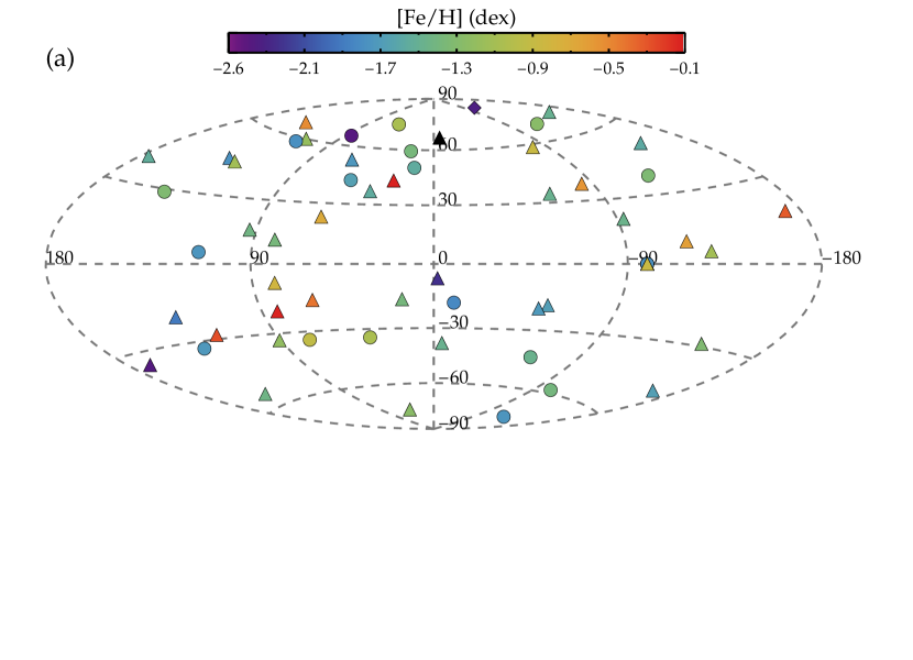
Figure 1: The sample of RR Lyrae Galactic Calibrators. (a) Distribution of targets in Galactic latitude ($l$) and longitude ($b$) color-coded by metallicity. Stars of type RRab are shown as triangles, RRc as circles, and RRd as a diamond. The target RR Lyrae are largely out of the Galactic plane ($|b|>10^{\circ}$), where variations in line-of-sight extinction due to dust variations are minimal (e.g., Zasowski et al., 2009). (b) Marginal distribution of [Fe/H] for our targets, demonstrating that the metal-poor end is well populated, but there are stars forming a high-metallicity tail. (c) Marginal distribution of $\log(P)$ for our targets, emphasizing a relatively uniform distribution.

2 The RR Lyrae Calibrator Sample

In this section we describe the demographics of our sample of 55 stars; a summary of the sample properties is given in Table 2.2. A comprehensive introduction to RRL is given by Smith (1995), with an updated presentation provided by Catelan & Smith (2015). As we describe our sample we briefly summarize the basics of RRL as needed for the purposes of this paper.

2.1 Demographics of Pulsation Properties

There are two primary subtypes of RRL, those that pulsate in the fundamental mode (RRab) and those that pulsate in the first overtone mode (RRc; i.e., there is a pulsational node within the star). A third subtype pulsates in both modes simultaneously — these are known as RRd-type variables. Generally, for stars of the same density, the ratio of the fundamental period ($P_{F}$) and the first-overtone period ($P_{FO}$) is approximately $P_{FO}$/$P_{F}$ = 0.746 (or $\Delta[\log(P)]=0.127$) and for many purposes the first overtone period can be converted to the equivalent fundamental period using this relationship. Application of this shift is often termed “fundamentalizing the period.” While RRab stars on average have longer periods than their first-overtone counterparts, the classification of a given star is generally based on the shape and amplitude of the optical light curve, with RRab stars having, in general, larger amplitudes and an asymmetric, ‘saw-tooth’ shape and RRc stars looking significantly more symmetric and sinusoidal. The distribution of RRL into these classifications is correlated with the specific (color/temperature) location of the star within the instability strip, which in turn is determined by where the star lands on the horizontal branch based on its post He-flash stellar structure and mass loss. RRc are hotter (bluer) than RRab, and the RRd-type stars fall in the color/temperature transition region between these two groupings. Based on their published classifications in the literature, 37 stars in our sample pulsate in the fundamental mode (RRab, 67%), 17 are in the first-overtone mode (RRc, 31%), and one star, CU Com, is a double-mode pulsator (RRd, 2%).

While many individual RRL have stable pulsation properties, as a population they can show modulation effects in the shapes and amplitudes of their light curves and in their periods. Light-curve modulations range both in their amplitudes — some even at the millimagnitude (only detectable with the exquisite time resolution and photometric stability for projects like Kepler in space and OGLE from the ground; see Nemec et al., 2013; Smolec et al., 2015, respectively) and some at the level of tenths of a magnitude (e.g., those discussed in Smith, 1995)—and in their timescales — some with very short few-day periods (e.g., Nemec et al., 2013) and some with very long multi-year periods (e.g., Skarka, 2014). The most famous of these is the Blazhko effect Blažko (1907), which is a periodic modulation of the amplitude and shape of an RRL light curve, with periods of order of tens to hundreds of pulsation cycles. The amplitude modulation from the Blazhko effect varies from star to star (and by passband) with ranges of a few hundredths to several tenths of a magnitude.

In addition, RRL stars can show period changes thought to correspond to the evolutionary path of an individual star. Such changes can appear to be sudden or gradual, depending on the time sampling of data sets. Recent efforts have combined temporally well-sampled, long-baseline photometric data sets in Galactic star clusters to explore these effects and find that most period changes ascribed to evolutionary effects are consistent with being gradual when visualized with semicontinuous sampling over very long timescales. Period changes attributed to nonevolutionary origins are also observed, and in contrast to evolutionary effects, these are identified as sudden nonlinear or chaotic evolution of the light curve over time (for example see Arellano Ferro et al., 2016, for a century-long study of period changes in M5). In our sample, nine stars show the Blazhko effect from Smith (1995, 16%; their Table 5.2), an additional four stars show the Blazhko effect from the compilation of Skarka (2013, 7%;), and two stars show the Blazhko effect in Skarka (2014, 4%), for a total of 15 stars showing the Blazhko effect. References for the studies demonstrating the Blazhko effect are given for each affected star in Appendix B.

The total frequency of Blazhko stars in our sample, 27%, is comparable to that observed for the full field RR Lyrae population and in clusters (e.g., Smith, 1995, though recent work has suggested this number could be as high as 50% when small amplitude variations are included; J. Jurcsik, private communication). The Blazhko periods for our sample (see Table 2.2) range from tens of days to several years and have Blazhko amplitudes that can be as small as only a few hundredths of a magnitude or as large as a few tenths of a magnitude. In our sample, 32% of our RRab stars are Blazhko (12 stars) and 18% of our RRc stars are Blazhko (3 stars); these frequencies are similar to but not perfectly matched to the general statistics for the Galactic RRL population, where $\sim$50% of RRab and $\sim$10% of RRc type variables show amplitude variations ( though we note the small number statistics for our RRc stars; for discussion see Section 6.5 of Catelan & Smith, 2015, and references therein). Considering our overall breakdown in RRL subtypes and amplitude modulation effects, the demographics of our RRL sample are not unrepresentative of the broader field population of Galactic RRL.

We note that our discussion has focused on stars with a single pulsation mode. In the era of space-based photometry and top-quality photometry gathered from Earth (e.g. Kepler from space and OGLE from the ground being two representative examples; see Nemec et al., 2013; Smolec et al., 2015, respectively), a more complicated view of RRL stars has emerged, and they can no longer be considered ‘simple’ radially pulsating stars. In 200 day continuous coverage for RRL in the M3 star cluster Jurcsik et al. (2015), find that 70% of RRc stars show multi-periodicity. Moreover, nonradial pulsation in RRc stars appears to be common because 14 out of 15 RRc stars (93%) observed from space show evidence for additional nonradial modes (e.g., Szabó et al., 2014; Moskalik et al., 2015; Molnár et al., 2015; Kurtz et al., 2016). Similarly, the incidence rate in the top-quality ground-based data is also large, with 27% of RRc in the OGLE Galactic bulge data (Netzel et al., 2015) and 38% in M3 photometry (Jurcsik et al., 2015) showing nonradial modes. Because many of these effects are of overall small amplitude, these nonradial modes and additional periodicities likely have a negligible effect on the goals of this work – to produce a robust Galactic calibration sample for parallax-based PL determinations – but do suggest that there is great complexity to the physical mechanisms at work in RRL stars. With these considerations in mind, an empirical approach to calibrating PL or PLZ relations is indeed preferable to theoretically derived relations that typically do not include the all of the physics driving these nonradial and multimode effects.

2.2 Effectiveness of Sample for PL Determinations

Figure 1(a) shows the sky distribution of the CRRP targets for Galactic coordinates. The stars span the complete range of R.A. and cover both hemispheres. The bulk of our sample of Galactic RRL reside out of the Galactic plane, which reduces complications from large line-of-sight extinction and variations of the reddening law within the disk (e.g., Zasowski et al., 2009, among others).

bf Figure 1(b) shows the [Fe/H] distribution of our catalog, spanning 2.5 dex in metallicity with the most metal poor star at $\text{[Fe/H]}=-2.56$ (UY Boo) and the most metal rich at $\text{[Fe/H]}=-0.07$ (AN Ser). The [Fe/H] values are adopted from the compilation of Fernley et al. (1998a) (as presented in Feast et al. (2008)) for all but two stars; the [Fe/H] for BB Pup comes from Fernley et al. (1998b) and that for CU Com from Clementini et al. (2000). The values from Fernley et al. (1998a) come from both direct high-resolution measurements and the $\Delta S$ method of Preston (1959), with the latter being calibrated to the former and brought onto a uniform scale having typical uncertainties of 0.15 dex. The majority of the sample can be considered metal poor with 70% (38 stars) of the sample uniformly distributed over a range of 1 dex ($-2<\text{[Fe/H]}<-1$) with a mean value of $\langle\text{[Fe/H]}\rangle=-1.50$ dex ($\sigma=0.24$ dex). The other 30% (17 stars) make up a metal rich sample that is itself uniformly distributed over a range of 1 dex ($-1<\text{[Fe/H]}<0$) with a mean value of $\langle\text{[Fe/H]}\rangle=-0.50$ dex ($\sigma=0.30$ dex).

Figure 1(c) shows the period distribution of our sample, with the shortest period being $P=0.25$ days (DH Peg) and the longest $P=0.73$ days (HK Pup) ($\log(P)=-0.60$ and $\log(P)=-0.14$, respectively). The sample is well designed to uniformly cover the distribution of $\log(P)$ anticipated in RRL populations and provide the greatest leverage to determine RRL relationships with respect to period.

With the exception of CU Com and BB Pup, all of our stars were included in the Hipparcos catalog (albeit with fractional errors larger than 30%), which means most stars were included in the Tycho-Gaia Astrometric Solution catalog (TGAS; Michalik et al., 2015; Lindegren et al., 2016) as part of Gaia DR1 Gaia Collaboration (2016); Gaia Collaboration et al. (2016). All five RR Lyrae from the Hubble Space Telescope-Fine Guidance Sensor parallax program presented in Benedict et al. (2011) are included in our sample. Seventeen stars have distances derived previously from the Baade-Wesselink (BW) technique in the recent compilation of Muraveva et al. (2015, and references therein). An additional five stars have BW distances from other works (see Table 2.2). The last three columns of Table 2.2 summarize the available distance measurements on a star-by-star basis.

Table 1: RRL Galactic Calibrators and Ephemerides.

Name	$P_{\text{final}}$	HJD${}_{\text{max}}$	$\zeta$	RRL Type	PBl	[Fe/H]	$\pi$
	(days)	(days)	(days yr-1)				HIP	BW	HST
SW And	0.4422602	2456876.9206	1.720e-04	RRab	36.8	-0.24	HIP	1,2
XX And	0.722757	2456750.915	$\cdots$	RRab	$\cdots$	-1.94	HIP
WY Ant	0.5743456	2456750.384	-1.460e-04	RRab	$\cdots$	-1.48	HIP	3
X Ari	0.65117288	2456750.387	-2.40e-04	RRab	$\cdots$	-2.43	HIP	4,5
ST Boo	0.622286	2456750.525	$\cdots$	RRab	284.0	-1.76	HIP
UY Boo	0.65083	2456750.522	$\cdots$	RRab	171.8	-2.56	HIP
RR Cet	0.553029	2456750.365	$\cdots$	RRab	$\cdots$	-1.45	HIP	1
W Crt	0.41201459	2456750.279	-9.400e-05	RRab	$\cdots$	-0.54	HIP	3
UY Cyg	0.56070478	2456750.608	$\cdots$	RRab	$\cdots$	-0.80	HIP
XZ Cyg	0.46659934	2456750.550	$\cdots$	RRab	57.3	-1.44	HIP		HST
DX Del	0.47261673	2456750.248	$\cdots$	RRab	$\cdots$	-0.39	HIP	2,8
SU Dra	0.66042001	2456750.580	$\cdots$	RRab	$\cdots$	-1.80	HIP	1	HST
SW Dra	0.56966993	2456750.400	$\cdots$	RRab	$\cdots$	-1.12	HIP	5
RX Eri	0.58724622	2456750.480	$\cdots$	RRab	$\cdots$	-1.33	HIP	1
SV Eri	0.713853	2456749.956	$\cdots$	RRab	$\cdots$	-1.70	HIP
RR Gem	0.39729	2456750.485	$\cdots$	RRab	7.2	-0.29	HIP	1
TW Her	0.399600104	2456750.388	$\cdots$	RRab	$\cdots$	-0.69	HIP	5
VX Her	0.45535984	2456750.405	-2.400e-04	RRab	455.37	-1.58	HIP
SV Hya	0.4785428	2456750.377	$\cdots$	RRab	63.3	-1.50	HIP
V Ind	0.4796017	2456750.041	$\cdots$	RRab	$\cdots$	-1.50	HIP
RR Leo	0.4523933	2456750.630	$\cdots$	RRab	$\cdots$	-1.60	HIP	1
TT Lyn	0.597434355	2456750.790	$\cdots$	RRab	$\cdots$	-1.56	HIP	1
RR Lyr	0.5668378	2456750.210	$\cdots$	RRab	39.8	-1.39	HIP		HST
RV Oct	0.5711625	2456750.570	$\cdots$	RRab	$\cdots$	-1.71	HIP	3
UV Oct	0.54258	2456750.440	$\cdots$	RRab	144.0	-1.74	HIP		HST
AV Peg	0.3903747	2456750.518	$\cdots$	RRab	$\cdots$	-0.08	HIP	1
BH Peg	0.640993	2456750.794	$\cdots$	RRab	39.8	-1.22	HIP
BB Pup	0.48054884	2456750.102	$\cdots$	RRab	$\cdots$	-0.60		3
HK Pup	0.7342073	2456750.387	$\cdots$	RRab	$\cdots$	-1.11	HIP
RU Scl	0.493355	2456750.296	$\cdots$	RRab	23.9	-1.27	HIP
AN Ser	0.52207144	2456750.334	$\cdots$	RRab	$\cdots$	-0.07	HIP
V0440 Sgr	0.47747883	2456750.706	$\cdots$	RRab	$\cdots$	-1.40	HIP	6
V0675 Sgr	0.6422893	2456750.819	$\cdots$	RRab	$\cdots$	-2.28	HIP
AB UMa	0.59958113	2456750.6864	$\cdots$	RRab	$\cdots$	-0.49	HIP
RV UMa	0.46806	2456750.455	$\cdots$	RRab	90.1	-1.20	HIP
TU UMa	0.5576587	2456750.033	$\cdots$	RRab	$\cdots$	-1.51	HIP	1
UU Vir	0.4756089	2456750.0557	-9.300e-05	RRab	$\cdots$	-0.87	HIP	1,5
AE Boo	0.31489	2456750.435	$\cdots$	RRc	$\cdots$	-1.39	HIP
TV Boo	0.31256107	2456750.0962	$\cdots$	RRc	9.74	-2.44	HIP	1
ST CVn	0.329045	2456750.567	$\cdots$	RRc	$\cdots$	-1.07	HIP
UY Cam	0.2670274	2456750.147	2.400e-04	RRc	$\cdots$	-1.33	HIP
YZ Cap	0.2734563	2456750.400	$\cdots$	RRc	$\cdots$	-1.06	HIP	6
RZ Cep	0.30868	2456755.135	-1.420e-03	RRc	$\cdots$	-1.77	HIP		HST
RV CrB	0.33168	2456750.524	$\cdots$	RRc	$\cdots$	-1.69	HIP
CS Eri	0.311331	2456750.380	$\cdots$	RRc	$\cdots$	-1.41	HIP
BX Leo	0.362755	2456750.782	$\cdots$	RRc	$\cdots$	-1.28	HIP
DH Peg	0.25551053	2456553.0695	$\cdots$	RRc	$\cdots$	-0.92	HIP	5,7
RU Psc	0.390365	2456750.335	$\cdots$	RRc	28.8	-1.75	HIP
SV Scl	0.377356	2457000.479	3.0e-04	RRc	$\cdots$	-1.77	HIP
AP Ser	0.34083	2456750.510	$\cdots$	RRc	$\cdots$	-1.58	HIP
T Sex	0.3246846	2456750.229	1.871e-03	RRc	$\cdots$	-1.34	HIP	1
MT Tel	0.3168974	2456750.108	5.940e-04	RRc	$\cdots$	-1.85	HIP
AM Tuc	0.4058016	2456750.392	$\cdots$	RRc	1748.9	-1.49	HIP
SX UMa	0.3071178	2456750.347	$\cdots$	RRc	$\cdots$	-1.81	HIP
CU Com	0.4057605	2456750.410	$\cdots$	RRd	$\cdots$	-2.38

References. — (1) Liu & Janes (1990); (2) Jones et al. (1992); (3) Skillen et al. (1993a); (4) Fernley et al. (1989); (5) Jones et al. (1988); (6) Cacciari et al. (1989); (7) Fernley et al. (1990); (8) Skillen et al. (1989)

3 The Three-hundred Millimeter Telescope

There are significant complications of a technical and practical nature when contemplating the use of traditional telescope/detector systems to study Galactic RRL. RRL have typical periods of order a day or less (requiring high-cadence, short-term sampling), but they can also show significant variations and period changes over time, requiring additional long-term sampling. These general considerations aside, the 55 Galactic RRL in our sample are noteworthy for being among the brightest RRL in the sky and are therefore too bright for even some of the “smallest” (i.e., 1 m class) telescopes at most modern observatories. Moreover, bright Galactic RRL are relatively rare and they are distributed over the entire night sky, which means that to build a uniform and relatively complete sample of such targets requires a dual-hemisphere effort. In direct response to this need, we assembled a devoted robotic 300mm telescope system to obtain modern, high-cadence, optical light curves for these important targets. In the sections to follow, we describe the telescope system (Section 3.1), the observing procedures (Section 3.2), and the resulting photometry (Section 3.3), with a summary given in Section 3.4.

3.1 TMMT Hardware

The Three-hundred MilliMeter Telescope (TMMT) is a 300mm $f/7.9$ flat-field Ritchey-Chrétien telescope on an AP1600 mount. The imager consists of an Apogee D09 camera assembly, which includes an E2V42-40 CCD with mid-band coatings and an external Apogee⁷ nine-position filter wheel containing U, B, V, R_c & I_c Bessel filters, a 7nm wide H$\alpha$ filter, and an aluminum blank acting as a dark slide. The imaging equipment is connected to the telescope via a Finger Lakes Instruments ATLAS focuser with adapters custom-made by Precise Parts. The short back focal length of the system and the depth of the CCD in the camera housing precluded the option of using an off-axis guider. For the program described here, individual exposures were short enough that guiding was not required. The mount contains absolute encoders, which are able to virtually eliminate periodic error, and the pointing model program applies differential tracking rates that correct for polar misalignment, flexure, and atmospheric refraction.

The system was first tested in the Northern Hemisphere at the Carnegie Observatories Headquarters (in downtown Pasadena, CA) from 2013 August to 2014 August. It was later (2014 September) shipped to Chile and permanently mounted in the Southern Hemisphere in a dedicated building with a remotely controlled, roll-off roof at Las Campanas Observatory (LCO). RRL monitoring observations continued until 2015 July.

The TMMT is controlled by a PC that can be accessed remotely through a VNC or a remote desktop sharing application. The unique testing and deployment of the TMMT has enabled true full-sky coverage for our RRL campaign, not just keeping the CCD setup consistent but also using the same system in both hemispheres so to minimize the effects of observational (equipment) systematics on our science goals.

3.2 Observations

ACP Observatory Control Software is used to automate the actions of the individual hardware components and associated software programs; more specifically, MaximDL controls the camera, FocusMax controls the focus, and APCC⁶ controls the mount. Weather safety information was obtained via the internet from the nearby HAT South facility .

For the RRL program, an ACP script was automatically generated each day to observe RRL program stars at phases that had not yet been covered. The script included observations of standard stars spaced throughout the night to calibrate the data. Additional scripts control other functions of the telescope, including: automatically starting the telescope at dusk, monitoring the weather, monitoring the state of each device and software to catch errors (and restart if necessary), and, finally, to shutting down at dawn. Images were automatically pipeline-processed using standard procedures, which are detailed in Appendix A.

The goal of the program was to obtain complete phase coverage for each of the 55 sources. Due to time and observability constraints, in particular the limited time available for the Northern sample while the telescope was deployed at the Carnegie Observatory Headquarters, there are still phase gaps for most of the stars. Additional phase sampling was obtained for nearly completed stars only when it was observationally efficient to do so. At the conclusion of the TMMT program, we have photometric observations in the $B$, $V$, and $I_{C}$ broadband filters for each of our 55 RRL.

Table 2: Optical Photometric Parameters for SBS and LCO.

Site	$v_{1}$	$v_{2}$	$v_{3}$	$b_{1}$	$b_{2}$	$b_{3}$	$i_{1}$	$i_{2}$	$i_{3}$
SBS	-4.18	0.23	-0.07	-0.44	0.14	1.32	0.78	0.08	0.92
$\sigma_{SBS}$	0.10	0.10	0.01	0.15	0.15	0.03	0.13	0.09	0.02
LCO	-4.09	0.13	-0.08	-0.42	0.10	1.32	0.68	0.08	0.92
$\sigma_{LCO}$	0.06	0.04	0.01	0.06	0.05	0.02	0.07	0.05	0.01

3.3 Photometry

Instrumental magnitudes ($m_{B}$, $m_{V}$, $m_{I_{C}}$) were extracted from the TMMT imaging data using DAOPHOT (Stetson, 1987). Aperture corrections were measured using DAOGROW (Stetson, 1990) and applied to correct the aperture photometry to infinite radius.

The magnitudes ($B$, $V$, $I_{C}$) and colors ($B-V$) and ($V-I_{C}$) for a set of standard stars were adopted from Landolt standard fields (Cousins, 1980; Landolt, 1983; Cousins, 1984; Landolt, 2009). Photometric calibrations were determined using the IRAF PHOTCAL package (Davis & Gigoux, 1993) with the fitparams and invertfit tasks. Second-order extinction terms were also measured, but found to be negligible and therefore not included.

The final adopted photometric calibration procedure is as follows: The zero-points are referenced to an airmass of 1.5 to minimize correlation between airmass ($X_{B}$, $X_{V}$, $X_{I_{C}}$) and zero-point terms. For the purposes of this work, we provide our calibrations for three of the photometric bands, $m_{B}$, $m_{V}$, $m_{I_{C}}$. We define relationships between these instrumental magnitudes and the true magnitudes ($B$, $V$, $I_{C}$) and colors ($B-V$, $V-I_{C}$) as follows:

$$V=v_{1}+m_{V}-v_{2}\left[(X_{V})-1.5\right]+v_{3}(m_{V}-m_{I_{C}})$$ (1)

$$B-V=b_{1}-b_{2}\left[0.5\times(X_{B}+X_{V})-1.5\right]+b_{3}(m_{B}-m_{V})$$ (2)

and

$$V-I_{C}=i_{1}-i_{2}\left[0.5\times(X_{I_{C}}+X_{V})-1.5\right]+i_{3}(m_{V}-m_{I_{C}})$$ (3)

The coefficients for the various corrections are: (i) zero-point offset ($b_{1}$, $v_{1}$, $i_{1}$), (ii) airmass term ($b_{2}$, $v_{2}$, $i_{2}$), (iii) and a color term ($b_{3}$, $v_{3}$, $i_{3}$). These three sets of coefficients (one set for each filter) are unique for the telescope and observing site. Median values and 1$\sigma$ deviations for the TMMT at the Carnegie Observatories Santa Barbara Street (SBS) and Las Campanas Observatory (LCO) sites are given in Table 2, and were used as the starting point for calibrating individual nights or were adopted as the solution if not enough standards were observed. Each photometric night has a systematic zero-point error determined from fitting the standard star photometry, which propagates to each RRL observed on that night. To reduce the final systematic uncertainty on the mean magnitude of an RRL, each RRL was observed on as many photometric nights as possible.

DAOMATCH and DAOMASTER were used to create the light curve relative to the first frame by finding and subtracting the average magnitude offset (determined from the ensemble photometry of common stars in all the frames) relative to the first frame in the series. Figure 2 shows the zero-point data for V Ind. The average differential magnitude ($\delta V$) for stars relative to the first frame is plotted with associated error bars. Since each frame was calibrated any frame taken on a photometric night could act as the reference, or alternatively, the average of all the photometrically calibrated frames can be used. The advantage of using the average is that it minimizes random fluctuations or poorly calibrated frames. Figure 2 illustrates an example where the first frame calibration deviated only slightly from the average. The final photometry is corrected by the average offset relative to the reference frame, thus avoiding the problem of choosing the “best” frame. Since multiple nights were used, each independently calibrated, the final systematic error is reduced. Note that the two nights plotted on the right of Figure 2 were not photometric and the default photometric solution was adopted. The transformation errors on nights such as this may appear discrepant if too few stars were used, resulting in potentially unrealistic photometric solutions; hence these nights are not used for calibration. Trends in nonphotometric data may be correlated with airmass, in which case the airmass term may be poorly constrained. Dips in the data may be due to a passing cloud or variable conditions.

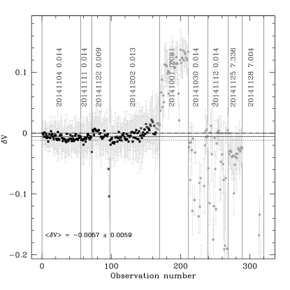
Figure 2: An example of the photometric errors over multiple nights for V Ind. A total of 326 images were reduced over nine nonconsecutive nights. Each frame is calibrated based on the transformation equations for that night. The average difference magnitude ($\delta V$) for stars relative to the first frame is plotted in with associated error bars. Four of the nights (black points) were photometric and had good photometric solutions from observations of standard star. The remaining nights either had poor solutions or used the default transformation coefficients. The systematic error of the nightly zero-point solution is given next to the date of observation; see text for details.

3.4 Summary

The TMMT is a fully robotic, 300 mm telescope at LCO, for which the nightly operation and data processing have completely automated. Over the course of two years data were collected on 179 individual nights for our sample of the 55 RR Lyrae in the $B$,$V$, and $I_{C}$ broadband filters. Of these nights, 76 were under photometric conditions and calibrated directly. The 103 nonphotometric nights were roughly calibrated by using the default transformation equations, but only provide differential photometry relative to the calibrated frames. This resulted in 59,698 final individual observations. Individual data points have a typical photometric precision of 0.02 mag. The statistical error falls rapidly with hundreds of observations, with the zero-point uncertainties being the largest source of uncertainty in the final reported mean magnitude.

4 Archival Observations

RR Lyrae variables can show changes in their periods (see discussions in Smith, 1995), and can have large accumulated effects from period inaccuracies, making it problematic to apply ephemerides derived from earlier work to new observational campaigns. While these two causes— period changes and period inaccuracies— have very different physical meanings (one intrinsic to the star and one to limited observations) the effect on trying to use data over long baselines is the same: individual observations will not “phase up” to form a self-consistent light curve. When well-sampled observations are available that cover a few pulsation cycles, it is possible to visually see the phase offset and simply align light-curve substructure (i.e., the exact timings of minimum and maximum light), but in the case of sparse sampling the resulting phased data will not necessarily form clear identifiable sequences (more details will be given in Section 5).

Thus, to compare the results of our TMMT campaign to previous studies of these RRL and to fill gaps in our TMMT phase coverage, we have compiled available broadband data from literature published over the past 30 years and spanning our full wavelength coverage. We note that this is not a comprehensive search of all available photometry. In the following sections, we give an overview of data sources for the sample, organized by passband, with star-by-star details given in Appendix B. Optical observations are described in Section 4.1, NIR observations in Section 4.2, and MIR observations in Section 4.3. Observations are converted from their native photometric systems to Johnson $U$, $B$, $V$, Kron-Cousins $R_{C}$,$I_{C}$, 2MASS $J,H,K_{s}$, and Spitzer 3.6$\mu$m and 4.5$\mu$m, with the transformations given in the text. Section 4.4 presents a summary of the resulting archival datasets.

4.1 Optical Data

4.1.1 ASAS

The All Sky Automated Survey (ASAS) is a long-term project monitoring all stars brighter than $V\sim$14 mag (Pojmanski, 1997, 2002, 2003; Pojmanski & Maciejewski, 2004, 2005; Pojmanski et al., 2005). The program covers both hemispheres, with telescopes at Las Campanas Observatory in Chile and Haleakala on Maui, both of which provide simultaneous $I$ and $V$ photometry. Not all photometry produced by the program has yet been made public (i.e., only $I$ or $V$ is available and for only limited fields and time frames). Moreover, several of our brightest targets, for example SU Dra and RZ Cep, both of which have parallaxes from the HST-FGS program, are not included. We adopt $V$ magnitudes from ASAS to augment phase coverage for some of our sample, if needed and where available.

4.1.2 GEOS

The Groupe Europ$e^{{}^{\prime}}$en d’Observations Stellaires (GEOS) RR Lyr Survey is a long-term program utilizing TAROT (Klotz et al., 2008, 2009) at Calern Observatory (Observatoire de la Côte d’Azur, Nice University, France). Annual data releases from this project add times for maximum light for program stars over the last year of observations (data releases include Le Borgne et al., 2005, 2006a, 2006b, 2007a, 2007b, 2008, 2009, 2011, 2013, among others). GEOS aims to characterize period variations in RRL stars by providing long-term, homogeneous monitoring of bright RRL stars, albeit only around the anticipated times of maximum light. The primary public data product from this program are the times of light curve maxima over a continuous period since the inception of the program in 2000. A well observed star will have its maximum identified to a precision of 4.3 minutes (0.003 days), but measurements vary between $\sigma_{max}$=0.002 and $\sigma_{max}$=0.010 days depending on local weather conditions. Such data are invaluable for understanding period and amplitude modulations for specific RRL (e.g., RR Lyr in Le Borgne et al., 2014) and for RRL as a population (Le Borgne et al., 2007c, 2012). We utilize the timing of maxima provided by GEOS for our common stars, primarily for the phasing efforts to be described in Section 5.

4.1.3 Individual Studies

In addition to the large programs previously described, we use data from individual studies over the past 30 years. Due to the diversity of such works, we must determine filter transformations on a study-by-study basis as we now describe.

For the conversion of Johnson $R_{J}$ and $I_{J}$ to Cousins $R_{C}$ and $I_{C}$ (noting that $V$ is the same in either), we utilize the following transformations from Fernie (1983):

$$V-R_{C}=\begin{cases}-0.024+0.730\times(V-R_{J})&\text{for }(V-R_{J})\leq 1.1\\ +0.218+0.522\times(V-R_{J})&\text{for }(V-R_{J})>1.1\end{cases}$$

and

$$R_{C}-I_{C}=\begin{cases}+0.034+0.845\times(R_{J}-I_{J})&\text{for }(R_{J}-I_{J})\leq 0.8\\ -0.239+1.315\times(R_{J}-I_{J})&\text{for }(R_{J}-I_{J})>0.8\end{cases}$$

$$V-I_{C}=\begin{cases}+0.004+0.783\times(V-I_{J})&\text{for }(V-I_{J})\leq 1.9\\ -0.507+1.217\times(V-I_{J})&\text{for }(V-I_{J})>1.9\end{cases}$$

This is required to convert data from Barnes et al. (1992) and Cacciari et al. (1987) to our system.

Optical data from Skillen et al. (1993b); Liu & Janes (1989); Paczyński (1965); Jones et al. (1992); Warren (1966); Fernley et al. (1990, 1989) and Clementini et al. (2000) are also used for our study but no global transformations were required.

4.2 Near-Infrared Data

Multi-Epoch data in the NIR are particularly sparse, but owing to numerous RRL campaigns in the 1980s and 1990s to apply the BW technique to determine distances to these stars, there are some archival data in these bands. Care, however, must be taken in using these archival data directly with more recent data, because (i) they must be brought onto the same photometric system (filter systems and detector technology have changed) and (ii) RRL are prone to period shifts over rather short time-scales. While the former concern can be characterized statistically, the latter concern presents a serious limitation to the use of archival data. Contemporaneous optical observations are necessary to properly phase the NIR data with our modern optical data. Thus, only data that could be phased, owing to the availability of contemporaneous optical data, could ultimately be used for our purposes.

4.2.1 2MASS

Single-epoch photometry is available from 2MASS (Skrutskie et al., 2006) in $J$, $H$, and $K_{s}$. Phasing of these data was accomplished primarily using data from GEOS (Section 4.1.2).

4.2.2 Individual Studies

Data from Sollima et al. (2008) are adopted and already on the 2MASS system.

To convert from the CIT systems to 2MASS we use the following transformations:

$$(J-K)_{\text{2MASS}}=1.068\times(J-K)_{\text{CIT}}-0.020\\ (H-K)_{\text{2MASS}}=1.000\times(H-K)_{\text{CIT}}+0.034\\ K_{s}=K_{\text{CIT}}-0.019+0.001\times(J-K)_{\text{CIT}}$$ (4)

This was required for data presented in Liu & Janes (1989), Barnes et al. (1992) and Fernley et al. (1993). If no color was provided, then the average color for RRL of $(J-K)_{\text{CIT}}$ = 0.25 was adopted.

The data in Skillen et al. (1989) and Fernley et al. (1990) required conversion from the UKIRT system as follows:

$$(J-K)_{\text{2MASS}}=1.070\times(J-K)_{\text{UKIRT}}-0.015\\ (H-K)_{\text{2MASS}}=1.071\times(H-K)_{\text{UKIRT}}+0.014\\ K_{s}=K_{\text{UKIRT}}+0.003+0.04\times(J-K)_{\text{UKIRT}}$$ (5)

The average colors for RRL of $(J-K)_{\text{UKIRT}}$ = 0.3 and $(H-K)_{\text{UKIRT}}$ = 0.1 were adopted if no color information data were available.

Data from Fernley et al. (1989) and Skillen et al. (1993a) required conversion from the SAAO system to 2MASS as follows:

$$(J-K)_{\text{2MASS}}=0.944\times(J-K)_{\text{SAAO}}-0.005\\ (H-K)_{\text{2MASS}}=0.945\times(H-K)_{\text{SAAO}}+0.043\\ K_{s}=K_{\text{SAAO}}-0.024+0.017\times(J-K)_{\text{SAAO}}$$ (6)

The average colors for RRL of $(J-K)_{\text{SAAO}}$ = 0.2 and $(H-K)_{\text{SAAO}}$ = 0.2 were adopted if no color data were available.

4.3 Mid-Infrared Data

4.3.1 Spitzer

The mid-infrared [3.6] and [4.5] (hereafter also S1 and S2, respectively) observations were taken using Spitzer/IRAC as part of the Warm–Spitzer Exploration Science Carnegie RR Lyrae Program (CRRP; PID 90002 Freedman et al., 2012). Each star was observed a minimum of 24 times (with additional observations provided by the Spitzer Science Center to fill small gaps in the telescope’s schedule). The Spitzer images were processed using SSC pipeline version S19.2. Aperture photometry was performed using the SSC-contributed software tool irac_aphot_corr, which performs the pixel-phase and location-dependent corrections. The photometry was calibrated to the standard system defined by Reach et al. (2005) using the aperture corrections for the S19.2 pipeline data provided to us by the SSC (S. Carey, 2016, private communication).

4.3.2 WISE

WISE (Wright et al., 2010) or NEOWISE (Mainzer et al., 2011, 2014) photometry is available for each of our stars (Wright et al., 2010). This is the only MIR data for three RRL. We opt to tie the WISE photometric system to that defined for Spitzer. For our RRL stars, we find an average offset of

$$W1-[3.6]=-0.038\pm 0.010$$ (7)

and

$$W2-[4.5]=-0.027\pm 0.010$$ (8)

This offset is applied to all of the WISE or NEOWISE data used in this work.

4.4 Summary of Archival Data

We have compiled a heterogeneous sample of data in order to build well sampled light curves from the optical to mid-infrared. We have homogenized these diverse data sets to the following filter systems: Johnson $UBV$, Kron-Cousins $RI$, 2MASS $J,H,K_{s}$, and Spitzer $[3.6]$, $[4.5]$. In addition to the photometric measurements, the phasing of the archival data had to be aligned to the current epoch because the periods of RRL can change over time; see Fig Figure 3 for examples of phase drift. Aligning the archival data in phase is the topic of Section 5.

Representative light curves for a subset of stars are shown in Figure 4. The stars shown in Figure 4 were selected based on having good sampling for the bulk of the 10 photometric bands. Individual data points are given in the first phase cycle of the data ($0<\phi<1$), with filled symbols being new data from this work (TMMT and Spitzer) and open symbols representing data taken from the literature. Single-epoch 2MASS data are represented by open pentagons. NIR data from Fernley et al. (1993) are available for many stars but only for a few epochs; these data are represented by open triangles. All other literature data in the NIR are represented by open squares.

Visualizations of this type are provided for each of our 55 stars as a figure set associated with Figure 4.

Figure 3: Data from GEOS (Sec 4.1.2) demonstrating of phasing solutions in the O-C diagram (see Section 5.1 for details) for the four cases described in the text. The solid vertical line highlights the epoch of the TMMT data and the vertical dashed line is at the epoch of the 2mass observations. (a) – top left Flat O-C behavior (for AN Ser) implies that no updates to period are required. (b) – top right Linear O-C behavior over the last 30 years (for DX Del) implies that the period is slightly longer than originally determined. (c) – bottom left Quadratic O-C behavior (for X Ari) implies that the period itself has been changing over time. (d) – bottom right Chaotic O-C behavior (for RR Lyr) implies that neither adding precision to the period nor applying a shift in period is sufficient to phase all of the individual data-sets analytically. In this case, each data-set gets a custom phase offset for alignment to the current TMMT epoch.

5 Reconciling Phase

Due to their short periods, RRL experience hundreds to over one thousand period cycles over a single year (between 500 and 1460 cycles per annum for our longest- and shortest-period RRLs, HK Pup and DH Peg, respectively). On these long timescales RR Lyrae can show physical changes in their periods due to their own stellar evolution that may appear gradual/smooth or sudden or they can show sudden changes with unexplained origins (i.e., changes not based on evolution). Over our 30 year baseline, a period uncertainty of 1 s results in maximal offsets of 0.17 day or a 0.24 phase for HK Pup (longest period) and 0.50 day or 1.95 full cycles for DH Peg (shortest period). Each individual observation taken within this time span would have its own phase offset. In this section, we describe our procedures to merge the data described in the previous section by updating the ephemerides for each star.

For clarification, we define several terms for the discussions to follow. A data set is either a single or a set of individual photometric measurement(s) for a given star and the associated date of observation taken with the same instrument setup and transformed into our standard photometric systems. We define the HJD${}_{\text{max}}$ as the HJD at maximum light measured from our TMMT data, which means that the quantity is defined uniformly for all stars in our sample. Our term ($\vartheta$) is the offset in days between our HJD${}_{\text{max}}$ and the date of observation, which is defined mathematically as follows:

$$\vartheta_{i}=\text{HJD}_{i,\text{obs}}-\text{HJD}_{\text{max}}$$ (9)

for each individual data point ($i$). Then, we define the initial phase ($\phi^{0}$) for each data point ($i$) as follows:

$$\phi^{0}_{i}=\frac{\vartheta_{i}}{P_{\text{archival}}}-\rm{int}{\left(\frac{\vartheta_{i}}{P_{\text{archival}}}\right)},$$ (10)

where the $P_{\text{archival}}$ is adopted from Feast et al. (2008). As we merge data, the initial phase ($\phi^{0}$) may be modified by adjustments to the period, HJD${}_{\text{max}}$, and inclusion of higher-order terms, which are fixed for an individual star. The final phase ($\phi$) for any given data point is defined as:

$$\phi_{i}=\frac{\vartheta_{i}}{P_{\text{final}}}-\rm{int}{\left(\frac{\vartheta_{i}}{P_{\text{final}}}\right)}+\zeta\left(\frac{\vartheta_{i}}{365.25}\right)^{2},$$ (11)

where $P_{\text{final}}$ is the final period, and $\zeta$ is an optional term (quadratic in $\vartheta$) that is used to describe changes in period in recent times, where $\zeta=0$ for a star with a stable period. The HJD${}_{\text{max}}$ measured from our TMMT data and $\zeta$ and $P_{\text{final}}$, determined by the analyses to follow, are given in Table 2.2 for each of the stars in our sample.

Our goal for this work is to build multi-wavelength light curves, and as such our goal for phasing is to make all of the data sets for a given star conform to a single set of HJD${}_{\text{max}}$, $P_{\text{final}}$ and $\zeta$ that self-consistently phase all of the data-sets for a star (see Appendix B). While this seems straightforward, in practice it is quite difficult owing both (i) to the nature of the observational data and (ii) to the nature of finding phasing solutions.

Based on the sampling, each observational data set can be placed into one of three categories:

• Case 1 —well sampled light curves,

• Case 2 —sparse coverage (or single points) for which there is a contemporaneous data set in the previous category (sparse data become ‘locked’ to the data in Case 1), and

• Case 3 —sparse coverage (or single points) with wide time baselines from well sampled curves.

Case 1 and Case 2 can be analyzed and evaluated in the O-C diagram, which compares the observed (O) and computed or predicted (C) time of maximum or minimum light as a function of time (here we will use $\vartheta$). The Case 2 data-sets become ‘locked’ to their contemporaneous Case 1 data sets. Usually the well sampled data sets can be merged by visual examination of their light curves. For Case 3, the ephemerides for the majority of the well sampled data must be complete (e.g., the analyses for Case 1 and Case 2) before the data set can be fully evaluated for consistency with the phased data sets. Usually, the Case 3 data set is ‘locked’ to the nearest GEOS maxima observation and phased to other data via small shifts in $\phi$.

5.1 The O-C Diagram

Full evaluation of the ephemerides occurs within the context of the O-C diagram (see Figure 3 of Liska & Skarka, 2015, for good demonstrations of various behaviors). O-C diagrams have a long history, beginning with Luyten (1921) and Eddington & Plakidis (1929), and are utilized for a number of time-domain topics in astronomy. An excellent general introduction to O-C diagrams and their application for various science goals, as well as detailed discussion of misuse of such diagrams, is provided by Sterken (2005) and we refer the interested reader to that text. We now describe our use of the O-C diagram in the context of the goals of this work.

The O-C diagrams for stars in our study could be classified into four characteristic behaviors, which are demonstrated in the panels of Figure 3: flat, linear, quadratic, and chaotic/jittery. These behaviors are applied to when the the data directly used in this study were taken. DX Del (Figure 3(b)), for example, was flat and then became (positive) linear; the linear portion applies to all available data analyzed in this work. None of the stars exhibited high-order periodic behavior that could be associated with a close companion or other complicated physical scenario (for examples of these cases see discussions in Sterken, 2005; Liska & Skarka, 2015). We discuss the implications for each of the situations in the sections to follow.

Flat O-C Diagram. If the data sets are in phase with the literature period and TMMT HJD${}_{\text{max}}$, then the O-C diagram will show flat behavior as in the example in Figure 3a. Physically, this means that the period itself has been stable over the time frame of the data set. If the TMMT HJD${}_{\text{max}}$ is correct, then $\langle O-C\rangle=0$; if it is incorrect, then there will be a zero-point offset. To reconcile, we adjust HJD${}_{\text{max}}$, where a positive (negative) offset implies that the observed HJD${}_{\text{max}}$ is occurs later (earlier) than the value predicted by Equation 10. HJD${}_{\text{max}}$ is then adjusted such that the $\langle O-C\rangle=0$.

Linear O-C Diagram. If the data sets show linear behavior (with nonzero slope) in the O-C diagram then observed maxima occur earlier (later) than predicted by Equation 10. This is typically an indication that the period is incorrect in a way that accumulates over time, i.e., a constant difference between the true period and that initially used for phasing. The magnitude of the slope provides the amount of period mismatch and the sign of the slope indicates whether the period should be lengthened (negative) or shortened (positive).

Quadratic O-C Diagram. RRL with historical or current constant period changes (most likely due to evolution) will have parabolic behavior in the O-C diagram. An upward (downward) parabola represents a period that is lengthening (shortening) at a constant rate over time. Since the period is still evolving, we describe the evolution of the period with an additional term in lieu of providing the period for the current epoch (if the period became constant, then we would see discontinuity from a parabola to linear). An example is given in Figure 3c. The quadratic shape can be fit, resulting in an additional coefficient for phasing the data, which we call $\zeta$ in Equation 10. Values of $\zeta$ are given in Table 2.2, with ‘no data’ indicating that no quadratic term was required.

Chaotic/Jittery O-C Diagram. Chaotic/jittery O-C diagrams could have many causes, including unresolved high-order variations due to companions, sudden period changes due to stellar evolution or other physical processes, typographical or computational errors in literature observations, and/or a combination of effects that cannot be identified individually (see some examples of individual effects in Liska & Skarka, 2015). Additionally, both sudden and prolonged chaotic and/or nonlinear effects could have causes unrelated to the physical evolution of the star. Merging data in these cases is quite complex. Our general approach is to fit only the recent behavior in the O-C diagram to adjust the ephemerides (the last decade is usually covered by GEOS). Older data sets are then treated individually, often requiring individual phase shifts for merging. An example chaotic/jittery O-C diagram is given in Figure 3d and for this demonstration we use RR Lyr itself, which appears chaotic/jittery in this visualization because of its strong Blazhko effect with a variable period (see Section B.33 for details).

5.2 Final Ephemerides

Making the data sets align to a single set of ephemerides is a multi-step process. Data are converted to an initial phase ($\phi_{0}$) based on the literature period ($P_{\text{archival}}$) and TMMT HJD${}_{\text{max}}$ using Equation 10. Iteration on the parameters occurs via visual inspection of the light curves from multiple data sets and the O-C Diagram. Case 1 and Case 2 data-sets provide the most leverage on the ephemerides and are, as such, merged first, with Case 3 data-sets being tied to the closest GEOS epoch and folded in last. Flat, linear, and quadratic O-C behaviors constrain adjustments to the ephemerides, which are also evaluated in the light curves. An additional term, $\zeta$, may be added as in Equation 11 to describe period changes in a quadratic O-C diagram. Final ephemerides are reported in Table 2.2, with some star-specific notes for chaotic/jittery O-C diagrams included in Appendix B.

Our final data sets report the final derived phase for each data point ($\phi_{i}$) using our adopted ephemerides as well as the original HJD of observation. Our process has generally preserved phase differences between filters. We note that our goal in this process was to build multi-wavelength light curves for the eventual multi-wavelength calibration of period-luminosity relationships and not to find the highest-fidelity ephemerides for these stars. Thus, while our solutions are adequate for our goal (as will be shown in the next section), they may not be unique solutions and may require further adjustment for other applications.

6 Light Curves and Mean Magnitudes

The light curves constructed from the newly acquired TMMT data and phased archival data are shown in Fig 4. The complete figure set (55 images) is available in Appendix B. The process of creating a light curve through the data using the GLOESS technique is described in the following sections. From the evenly sampled GLOESS light curve the intensity mean magnitude is determined as a simple average of the intensity of the GLOESS data points and converted to a magnitude. Table 6 contains each new TMMT measurement along with all phased archival data included in this study. The full table is available in the online journal and a portion is shown here for form and content.

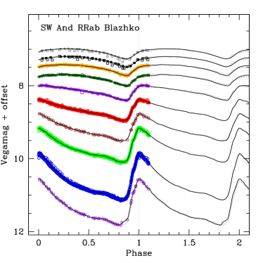
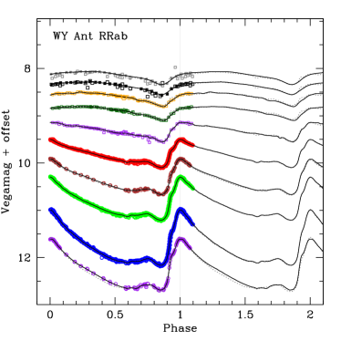
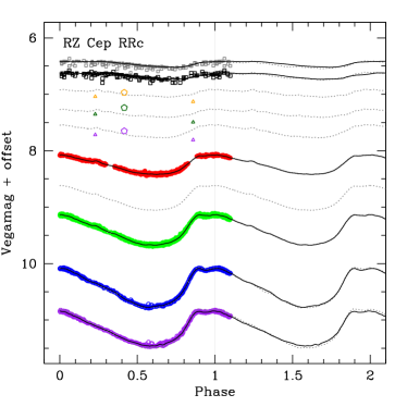
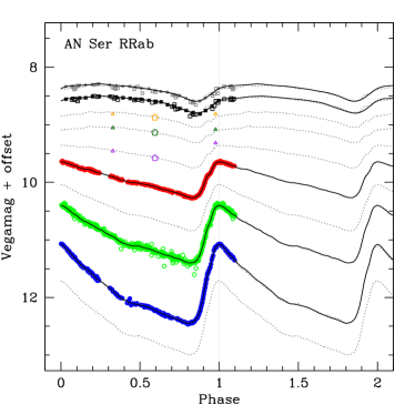
Figure 4: Example light curves from the final data sets. Data and GLOESS fits for the RRab types SW And (top left) and WY Ant (top right) and the RRc types RZ Cep (bottom left) and T Sex (bottom right). From top to bottom in each panel, the bands are $S2$ (gray), $S1$ (black), $K_{s}$ (orange), $H$ (dark green), $J$ (purple), $I_{C}$ (red), $R_{C}$ (brown), $V$ (light green), $B$ (blue), and $U$ (purple). Filled points are newly acquired data from TMMT (circles) and Spitzer (squares). All open symbols are adopted from the literature. Large open pentagons are $J$, $H$, $K_{s}$ from 2MASS, open triangles are NIR data from Fernley et al. (1993) and open squares are NIR data from the remaining literature sources. For the MIR data, open symbols are from WISE and filled symbols are from Spitzer. The GLOESS light curve fit for each band is shown as the solid line ($3\sigma$ outliers were rejected during creation of the GLOESS light curve). The dotted line is constructed from the $V$ and $I$ GLOESS light curves for each band. The process of generating this faux curve and using it as a template is the topic of a future paper, but is briefly demonstrated here.

Fig. Set4. Multi-Wavelength phased RR Lyrae light curves

Table 3: TMMT Photometry and Phased Archival Data

Star	Filter	mag	$\sigma_{phot}$	$\sigma_{sys}$	HMJD	Phase ($\phi$)	Reference
SW And	I	9.170	0.010	0.009	56549.3206	0.390	0
SW And	I	9.168	0.010	0.009	56549.3216	0.392	0
SW And	I	9.173	0.010	0.009	56549.3222	0.394	0
SW And	I	9.174	0.010	0.009	56549.3229	0.395	0
SW And	I	9.171	0.010	0.009	56549.3235	0.397	0

Note. — The Heliocentric Modified Julian Day (HMJD = HJD - 2400000.5) is provided. The photometric error for each measurement is included as well as the systematic error in the zero-point determination. Table 6 is published in its entirety in the machine-readable format. A portion is shown here for guidance regarding its form and content.

References. — (0) TMMT This work; (1) Spitzer This work; (4) Skillen et al. (1993a); (5) Barnes et al. (1992); (7) Liu & Janes (1989); (8) Liu & Janes (1989); (9) Barcza & Benkő (2014); (10) Paczyński (1965); (11) 2MASS Skrutskie et al. (2006); (17) ASAS Pojmanski (1997); (15) Jones et al. (1992); (19) IBVS Broglia & Conconi (1992); (31) Fernley et al. (1990); (41) Fernley et al. (1989); (98) Clementini et al. (1990); (99) Clementini et al. (2000); (999) TMMT modified for Blazhko effect.

6.1 GLOESS Light Curve Fitting

Nonparametric kernel regression and local polynomial fitting have a long history, dating as far back as Macaulay (1931); in particular they have been extensively applied to the analysis of time series data. More recently popularized and developed by Cleveland (1979) and Cleveland & J. (1988), this method has been given the acronym LOESS (standing for LOcal regrESSion), or alternatively and less frequently LOWESS (standing for LOcally WEighted Scatterplot Smoothing). In either event, a finite-sized, moving window (a kernel of finite support) was used to select data, which were then used in a polynomial regression to give a single interpolation point at the center of the adopted kernel (usually uniform or triangular windows). The kernel was then moved by some interpolation interval determined by the user and the process repeated until the entire data set was scanned. Instabilities would occur when the window was smaller than the largest gaps between consecutive data points. To eliminate this possibility one of us (BFM) introduced GLOESS, a Gaussian-windowed LOcal regrESSion method, first used by Persson et al. (2004) to fit Cepheid light curves. In its simplest form GLOESS penalized the data, both ahead of and behind the center point of the window, by their Gaussian-weighted distance quadratically convolved with their individual statistical errors. Instabilities are guaranteed to be avoided given that all data contribute to the polynomial regressions at every step.

GLOESS light curves were created for our stars for each band independently, the goal being to create uniformly interpolated light curves from nonuniformly sampled data. In this way, for example, color curves and/or other more complicated combinations of colors and magnitudes can be derived from multi-wavelength data sets that were collected in different bands at disparate and non-overlapping epochs (see for example the application in Freedman & Madore, 2010). In our particular implementation of the GLOESS formalism the width of the window, $\Delta x$ (usually phase), could be either set to a constant or allowed to vary as the density of available data points changes. The latter allows for finer detail to be captured in the interpolation in regions where there are more densely populated data points. Our implementation has been extended further by also weighting in $\Delta y$ (magnitude). By doing a first-pass linear interpolation the data points are weighted by an additional factor of $e^{-\Delta_{y}^{2}/\sigma_{y}^{2}}$. In this way, regions near the top and bottom of a steeply rising feature are “shielded” from each other. In this case, $\sigma_{y}$ is the scatter in the data within the $\Delta x$ window. Outliers are clipped by performing a second iteration and rejecting points outside $3\sigma$. For some stars, it proved useful to partition the data into discrete regions to further isolate steeply changing features from one another.

The results of the GLOESS fitting are shown for each of the light curves given in Figure 4 as the solid gray lines. In comparison to the data points (shown for $0<\phi<1.0$), the GLOESS curve (shown in isolation for $1.0<\phi<2.0$) accurately traces the natural structure of the light curves with no a priori assumptions of that shape. There are two types of cases in our current sample that require special attention. These are (i) those stars exhibiting the Blazhko effect in our sampling (typically only visible in TMMT data) and (ii) those stars with large phase gaps.

6.1.1 Treatment of the Blazhko Effect

The Blazhko effect is a modulation of the amplitude and shape of the RRL light curve with periods ranging from a few to hundreds of days. The search for a physical basis for the Blazhko effect remains unclear globally and is beyond the scope of this paper. The average luminosity of Blazhko stars remains constant from cycle to cycle; however; data that nonuniformly sample the light curve from different Blazhko cycles may lead to an incorrect determination of the mean, biased in the direction where most of the data were obtained. For the purposes of this paper, we did the following: If the observations could be separated cleanly into distinct Blazhko cycles, then the two cycles were shifted and scaled to one another if necessary for the purposes of GLOESS fitting (for example, SV Hya and RV UMa). Data displayed in these figures are the original photometry with the modified photometry displayed in gray. If the observations could not readily be separated, then the GLOESS algorithm was left to average between the cycles.

6.1.2 Light-curve Partitioning

One feature of GLOESS is that points ahead of or behind the current interpolation point are downweighted. In the optical bands, the light curves can have very rapid rise times, and even with the the weighting function sometimes the data on the ascending or descending side of the light curve still influence the local estimation of the others. Here we briefly discuss the general modification of GLOESS for these situations.

For the purposes of this work, the phase between minimum light and just past maximum light was often ‘partitioned’ such that the points on either side of the maximum could not influence each other. This partitioning was particularly necessary for the optical light curves of RRab variables. This was done by setting the weights of those points outside the fitting partition to zero. To prevent discontinuities at or near the partition point, data from within 0.02 in phase were allowed to contribute from the opposite side. In this way, there were always data to interpolate and GLOESS did not have to extrapolate.

Another feature of GLOESS is that at each point of interpolation a quadratic function locally fits the weighted data. This low-order function has the advantage of not overfitting the data and generally changes slowly at adjacent interpolation points, thus providing a relatively smooth and continuous curve through the data in the end. At the timing of the ‘hump’ in the ascending branch of the light curve for RRabs in the optical (see Chadid et al., 2014, Figure 6 for a visualization), the function is allowed to use the best $\chi^{2}$ result for a first-, second-, or third-order order polynomial. Because the ‘hump’ happens so quickly there are often not enough data to capture the subtlety of the feature. Allowing for a third-order polynomial in this region avoids losing this and similar features in the light curves. RRcs are relatively smooth (in comparison to RRabs) and we always use an underlying quadratic function.

6.2 Light-curve Properties

Mean magnitudes were determined by computing the mean intensity of the evenly sampled GLOESS fit points to the light curve, then converting back to a magnitude. The light curve must be sampled with enough data points to capture all the nuances of the shape for an accurate mean; in our case we sampled with 256 data points spaced every 1/256 in phase. Generally, GLOESS fits were determined only for those stars and bands that had more than 20 individual data points over a reasonable portion of phase (i.e., 20 data points only spanning $\phi\sim$ 0.1 would not have a GLOESS fit nor a mean magnitude). Table 4 contains each GLOESS-generated light curve. The full table is available in the online journal and a portion is shown here for form and content.

The random uncertainty of the GLOESS-derived mean magnitude is simply the error on the mean of data points going into GLOESS fitting. Thus, stars with more data points will have a smaller uncertainity in GLOESS mean magnitude. The systematic uncertainty is determined by the photometric transformations, either in transforming our TMMT photometry onto an absolute system (see Figure 2) or as reported in the literature and in transforming from other filter systems (as described in Section 4). The final reported error is $\sigma^{2}=1/\sum(1/\sigma_{phot}^{2})+1/\sum(1/\sigma_{sys}^{2})$, where the sum over $\sigma_{sys}$ includes only the unique entries from each reference, i.e. it is not counted for every measurement. These results are given in Table Acknowledgments. A technique to better utilize sparsely sampled data will be presented in a future companion paper (R. L. Beaton et al. 2017,  in preparation) and no mean magnitudes are reported here for data with too few measurements to construct a GLOESS light curve.

In addition to the mean magnitudes, we provide amplitudes ($a_{\lambda}$), rise times ($RT_{\lambda}$), and magnitudes at HJD${}_{\text{max}}$ in Table LABEL:tab:lcpars as measured from the GLOESS light curves. We define ($a_{\lambda}$) and ($RT_{\lambda}$) as the difference in magnitude and phase, respectively, between the minimum and maximum of the GLOESS light curve. We note that at the longer wavelengths these terms become less well defined due to the less prominent ‘saw-tooth’ shape and overall smaller amplitudes, both of which are typical changes for RRL stars at these passbands.

Table 4: GLOESS light curves.

Star Name	Filter	$\phi$	GLOESS Mag.
SW And	U	0.00000	9.562
SW And	U	0.00391	9.559
SW And	U	0.00781	9.560
SW And	U	0.01172	9.563
SW And	U	0.01562	9.571

Note. — Table 4 is published in its entirety in the machine-readable format. A portion is shown here for guidance regarding its form and content.

6.3 Comparison with Literature Values

The difference between the intensity means in the $V$ band determined here and literature values is shown in Figure 5. In most cases $B$ photometry is available for comparison with respect to $V$ (i.e. $B-V$), but $I_{C}$ is not, which was part of the motivation for this work. Notable outliers are labeled in Figure 5 and it is worth noting that three out of the five RRL with HST parallaxes are considered outliers. Both RV UMa and ST Boo exhibit the Blazhko effect (our treatment of these stars was discussed in Section 6.1.1) and differences are likely due to having sampled different parts of the Blazhko cycle.

We compare our GLOESS-derived apparent mean magnitudes for 53 stars to those presented in Feast et al. (2008), which were originally derived in Fernley et al. (1998a) from Hipparcos Fourier fitting to $H_{P}$ magnitudes (converted to intensity). A correction was used in Fernley et al. (1998a) to transform the RRL from the $H_{P}$ system onto the standard Johnson $V$ system by adopting an average color for each subtype of star; the corrections were $-0.09$ mag for the RRabs and $-0.06$ mag for the RRcs. Some of the scatter from Feast et al. (2008) and Fernley et al. (1998a) in Figure 5 is due to reddening, since the corrections were not based on apparent color but rather by adopting a mean color for each type of star. RZ Cep (type RRc), for example, is highly reddened and has an apparent color redder than most RRabs (which should be intrinsically redder than RRcs). Thus RZ Cep’s (and the others’) color correction was likely underestimated when transforming from $H_{P}$ to $V$. Both XZ Cyg and RR Lyr are also offset, perhaps due to their Blazhko cycle. The mean magnitude from Fernie (1965) for RR Lyr is in agreement with the value determined here. For 51 stars in common (two rejected) we find an average offset of $\Delta V=-0.018\pm 0.021$ mag.

Piersimoni et al. (1993) provide photometry for two stars (AB UMa and ST Boo). There is good agreement on AB UMa, but the reported mean magnitude reported for ST Boo (a Blazhko star) differs by 0.07 mag.

There are a number of stars with BW analysis; the results of Skillen et al. (1993b, 1989) and Fernley et al. (1989, 1990) are grouped together in Fig 5 as ”Skillen 1993.” For the seven stars in common (one rejected), we find an average offset of $\Delta V=-0.005\pm 0.009$ magnitudes. W Crt was discussed in Skillen et al. (1993b) as perhaps having an offset from observations between different telescopes.

We have 10 stars in common with Liu & Janes (1990) and we we find an average offset of $\Delta V=-0.008\pm 0.007$ mag. For the 10 stars in common with Fernie (1965) we find an average offset of $\Delta V=-0.001\pm 0.016$ mag. For three stars in common with Cacciari et al. (1987, we exclude V0440 Sgr), we find an average offset of $\Delta V=-0.009\pm 0.001$ mag.

Simon & Teays (1982) adopted photometry for a number of stars from earlier sources to generate Fourier fits to the light curve for each star. The fits were performed in magnitudes so the Fourier parameters provided were used to generate light curves from which the intensity-averaged magnitudes were determined. For the 23 stars in common with Simon & Teays (1982), we find an average offset of $\Delta V=-0.019\pm 0.024$ mag.

Overall, the average offsets in the Johnson $V$ band between the literature intensity mean values in the literature and our current results fall between 1% and 2%. On average this would indicate that the current photometry is about 1% brighter than previous estimates. To check potential systematics, random standard stars observed with TMMT were processed like the RRL sample and the final mean magnitudes did not deviate from their standard values. Additionally, to check the GLOESS method, literature data was passed through the GLOESS algorithm and their final mean magnitudes agreed with their published values. The source of any systematic remains unclear and a full investigation into the potential systematics involved in the complete assimilation of other data from the literature is beyond the scope of this paper.

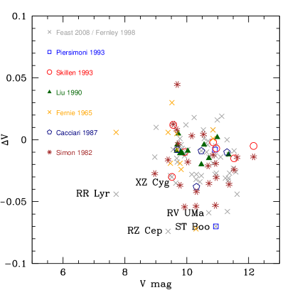
Figure 5: Difference between the current intensity mean values ¡$V$¿ and values published in the literature as described in the text.

7 Summary and Future Work

With the upcoming Gaia results, we will soon be able to calibrate the period–luminosity relationship directly using trigonometric parallaxes for a large sample of nearby Galactic RR Lyrae variables. In anticipation of the Gaia data releases, we have prepared a data set spanning a wavelength range from 0.4 to 4.5 microns in 10 individual photometric bands for a sample of 55 bright, nearby RR Lyrae variables that will be in the highest-precision Gaia sample. Moreover, 53 of the 55 stars appear in the Hipparcos catalog, and a large fraction were a part of the Gaia first data release with the Tycho-Gaia Astrometric Solution (TGAS; Michalik et al., 2015; Lindegren et al., 2016). Our sample spans a representative range of RRL properties, containing both RRab and RRc type stars, a wide range of metallicity, and several stars showing short-term and long-term Blazhko modulations.

In this paper, we described the TMMT, an automated, small-aperture facility designed to obtain high-precision, multi-epoch photometry for calibration sources. We presented a multi-site and multi-year campaign with the TMMT that produced well-sampled optical light curves for our (55-star) sample. Additionally, we utilize MIR light curves obtained in the CRRP. Furthermore, we present an extensive literature search of the photometry to expand our phase coverage at all wavelengths. We described our efforts to merge these data sets to conform to a single set of ephemerides (HJD_max, period, and higher-order terms) and explicitly include both our filter transformations and phasing solutions.

With multi-wavelength merged data sets, we apply the GLOESS technique to produce well-sampled, smoothed light curves for as many stars and bands as possible. GLOESS produces light curves that are not scaled templates or analytic functions, but are generated from a stars’ actual data and thereby preserve the details of their often unique light-curve sub-structure. We describe adaptations of this technique required for application to stars with large amplitude modulations due to the Blazhko effect, and with other light -curve features that can present challenges. The GLOESS light curves are then used to determine high-precision intensity mean magnitudes and mean light-curve properties including amplitudes, rise times, and magnitudes at minimum and maximum light.

While our study is as complete as possible, many stars have observational data that are currently not well sampled enough for the direct application of GLOESS. We have GLOESS light curves for 22 (40%) stars in the $U$, 55 (100%) stars in $B$, 55 (100%) stars in $V$, 20 (36%) stars in $R$, 55 (100%) stars in $I$, 19 (35%) stars in $J$, 9 (16%) stars in $H$, 20 (36%) stars in $K_{s}$, 55 (100%) in [3.6], and 55 (100%) in [4.5]. Our sample is particularly limited for the near-infrared, where high-cadence observations of bright stars are challenging or observationally expensive. A companion paper will present a technique, schematically described in Beaton et al. (2016), that uses the TMMT-derived GLOESS optical light curves presented in this work to produce star-by-star predictive templates capable of making use of single-phase or sparsely sampled data sets for RR Lyrae.

References

- Arellano Ferro et al. (2016) Arellano Ferro, A., Ahumada, J. A., Kains, N., & Luna, A. 2016, MNRAS, arXiv:1606.01181
- Baade (1926) Baade, W. 1926, Astronomische Nachrichten, 228, 359
- Barcza & Benkő (2014) Barcza, S., & Benkő, J. M. 2014, MNRAS, 442, 1863
- Barnes et al. (1992) Barnes, III, T. G., Moffett, T. J., & Frueh, M. L. 1992, PASP, 104, 514
- Beaton et al. (2016) Beaton, R. L., Freedman, W. L., Madore, B. F., et al. 2016, ArXiv e-prints, arXiv:1604.01788
- Benedict et al. (2011) Benedict, G. F., McArthur, B. E., Feast, M. W., et al. 2011, AJ, 142, 187
- Blažko (1907) Blažko, S. 1907, Astronomische Nachrichten, 175, 325
- Braga et al. (2015) Braga, V. F., Dall’Ora, M., Bono, G., et al. 2015, ApJ, 799, 165
- Broglia & Conconi (1992) Broglia, P., & Conconi, P. 1992, Information Bulletin on Variable Stars, 3748
- Cacciari et al. (1989) Cacciari, C., Clementini, G., & Buser, R. 1989, A&A, 209, 154
- Cacciari et al. (1987) Cacciari, C., Clementini, G., Prevot, L., et al. 1987, A&AS, 69, 135
- Catelan & Smith (2015) Catelan, M., & Smith, H. A. 2015, Pulsating Stars
- Chadid et al. (2014) Chadid, M., Vernin, J., Preston, G., et al. 2014, AJ, 148, 88
- Clementini et al. (1990) Clementini, G., Cacciari, C., & Lindgren, H. 1990, A&AS, 85, 865
- Clementini et al. (2000) Clementini, G., Di Tomaso, S., Di Fabrizio, L., et al. 2000, AJ, 120, 2054
- Cleveland (1979) Cleveland, w. S. 1979, Journal of the American Statistical Association, 74, 829. http://www.jstor.org/stable/2286407
- Cleveland & J. (1988) Cleveland, W. S., & J., D. S. 1988, Journal of the American Statistical Association, 83, 596. http://www.jstor.org/stable/2289282
- Cousins (1980) Cousins, A. W. J. 1980, South African Astronomical Observatory Circular, 1, 234
- Cousins (1984) —. 1984, South African Astronomical Observatory Circular, 8, 69
- Dall’Ora et al. (2004) Dall’Ora, M., Storm, J., Bono, G., et al. 2004, ApJ, 610, 269
- Davis & Gigoux (1993) Davis, L. E., & Gigoux, P. 1993, in Astronomical Society of the Pacific Conference Series, Vol. 52, Astronomical Data Analysis Software and Systems II, ed. R. J. Hanisch, R. J. V. Brissenden, & J. Barnes, 479
- de Bruijne et al. (2014) de Bruijne, J. H. J., Rygl, K. L. J., & Antoja, T. 2014, in EAS Publications Series, Vol. 67, EAS Publications Series, 23–29
- Drimmel et al. (2003) Drimmel, R., Cabrera-Lavers, A., & López-Corredoira, M. 2003, A&A, 409, 205
- Eddington & Plakidis (1929) Eddington, A. S., & Plakidis, S. 1929, MNRAS, 90, 65
- Feast et al. (2008) Feast, M. W., Laney, C. D., Kinman, T. D., van Leeuwen, F., & Whitelock, P. A. 2008, MNRAS, 386, 2115
- Fernie (1965) Fernie, J. D. 1965, ApJ, 141, 1411
- Fernie (1983) —. 1983, PASP, 95, 782
- Fernley & Barnes (1997) Fernley, J., & Barnes, T. G. 1997, A&AS, 125, doi:10.1051/aas:1997222
- Fernley et al. (1998a) Fernley, J., Barnes, T. G., Skillen, I., et al. 1998a, A&A, 330, 515
- Fernley et al. (1998b) Fernley, J., Skillen, I., Carney, B. W., Cacciari, C., & Janes, K. 1998b, MNRAS, 293, L61
- Fernley et al. (1989) Fernley, J. A., Lynas-Gray, A. E., Skillen, I., et al. 1989, MNRAS, 236, 447
- Fernley et al. (1993) Fernley, J. A., Skillen, I., & Burki, G. 1993, A&AS, 97, 815
- Fernley et al. (1990) Fernley, J. A., Skillen, I., Jameson, R. F., & Longmore, A. J. 1990, MNRAS, 242, 685
- Freedman et al. (2012) Freedman, W., Scowcroft, V., Madore, B., et al. 2012, The Carnegie RR Lyrae Program, Spitzer Proposal, ,
- Freedman & Madore (2010) Freedman, W. L., & Madore, B. F. 2010, ApJ, 719, 335
- Gaia Collaboration (2016) Gaia Collaboration. 2016, ArXiv e-prints, arXiv:1609.04153
- Gaia Collaboration et al. (2016) Gaia Collaboration, Brown, A. G. A., Vallenari, A., et al. 2016, ArXiv e-prints, arXiv:1609.04172
- Hurta et al. (2008) Hurta, Z., Jurcsik, J., Szeidl, B., & Sódor, Á. 2008, AJ, 135, 957
- Jones et al. (1988) Jones, R. V., Carney, B. W., & Latham, D. W. 1988, ApJ, 332, 206
- Jones et al. (1992) Jones, R. V., Carney, B. W., Storm, J., & Latham, D. W. 1992, ApJ, 386, 646
- Jurcsik et al. (2005) Jurcsik, J., Sódor, Á., Váradi, M., et al. 2005, A&A, 430, 1049
- Jurcsik et al. (2009) Jurcsik, J., Sódor, Á., Szeidl, B., et al. 2009, MNRAS, 400, 1006
- Jurcsik et al. (2015) Jurcsik, J., Smitola, P., Hajdu, G., et al. 2015, ApJS, 219, 25
- Klotz et al. (2009) Klotz, A., Boër, M., Atteia, J. L., & Gendre, B. 2009, AJ, 137, 4100
- Klotz et al. (2008) Klotz, A., Vachier, F., & Boër, M. 2008, Astronomische Nachrichten, 329, 275
- Kolenberg et al. (2006) Kolenberg, K., Smith, H. A., Gazeas, K. D., et al. 2006, A&A, 459, 577
- Kolenberg et al. (2011) Kolenberg, K., Bryson, S., Szabó, R., et al. 2011, MNRAS, 411, 878
- Kollmeier et al. (2013) Kollmeier, J. A., Szczygieł, D. M., Burns, C. R., et al. 2013, ApJ, 775, 57
- Kurtz et al. (2016) Kurtz, D. W., Bowman, D. M., Ebo, S. J., et al. 2016, MNRAS, 455, 1237
- LaCluyzé et al. (2004) LaCluyzé, A., Smith, H. A., Gill, E.-M., et al. 2004, AJ, 127, 1653
- Landolt (1983) Landolt, A. U. 1983, AJ, 88, 439
- Landolt (2009) —. 2009, AJ, 137, 4186
- Le Borgne et al. (2005) Le Borgne, J. F., Klotz, A., & Boer, M. 2005, Information Bulletin on Variable Stars, 5622
- Le Borgne et al. (2006a) —. 2006a, Information Bulletin on Variable Stars, 5686
- Le Borgne et al. (2006b) —. 2006b, Information Bulletin on Variable Stars, 5717
- Le Borgne et al. (2007a) —. 2007a, Information Bulletin on Variable Stars, 5767
- Le Borgne et al. (2007b) —. 2007b, Information Bulletin on Variable Stars, 5790
- Le Borgne et al. (2008) —. 2008, Information Bulletin on Variable Stars, 5853
- Le Borgne et al. (2009) —. 2009, Information Bulletin on Variable Stars, 5895
- Le Borgne et al. (2011) —. 2011, Information Bulletin on Variable Stars, 5986
- Le Borgne et al. (2013) —. 2013, Information Bulletin on Variable Stars, 6043
- Le Borgne et al. (2007c) Le Borgne, J. F., Paschke, A., Vandenbroere, J., et al. 2007c, A&A, 476, 307
- Le Borgne et al. (2012) Le Borgne, J.-F., Klotz, A., Poretti, E., et al. 2012, AJ, 144, 39
- Le Borgne et al. (2014) Le Borgne, J. F., Poretti, E., Klotz, A., et al. 2014, MNRAS, 441, 1435
- Lindegren et al. (2016) Lindegren, L., Lammers, U., Bastian, U., et al. 2016, ArXiv e-prints, arXiv:1609.04303
- Liska & Skarka (2015) Liska, J., & Skarka, M. 2015, Open European Journal on Variable Stars, 169, 38
- Liu & Janes (1989) Liu, T., & Janes, K. A. 1989, ApJS, 69, 593
- Liu & Janes (1990) —. 1990, ApJ, 354, 273
- Liška et al. (2016) Liška, J., Skarka, M., Mikulášek, Z., Zejda, M., & Chrastina, M. 2016, A&A, 589, A94
- Longmore et al. (1990) Longmore, A. J., Dixon, R., Skillen, I., Jameson, R. F., & Fernley, J. A. 1990, MNRAS, 247, 684
- Longmore et al. (1986) Longmore, A. J., Fernley, J. A., & Jameson, R. F. 1986, MNRAS, 220, 279
- Luyten (1921) Luyten, W. J. 1921, Observations of variable stars …
- Macaulay (1931) Macaulay, F. R. 1931, The Smoothing of Time Series (New York, New York, USA: NBER). http://www.nber.org/books/maca31-1
- Mainzer et al. (2011) Mainzer, A., Bauer, J., Grav, T., et al. 2011, ApJ, 731, 53
- Mainzer et al. (2014) Mainzer, A., Bauer, J., Cutri, R. M., et al. 2014, ApJ, 792, 30
- Michalik et al. (2015) Michalik, D., Lindegren, L., & Hobbs, D. 2015, A&A, 574, A115
- Molnár et al. (2015) Molnár, L., Szabó, R., Moskalik, P. A., et al. 2015, MNRAS, 452, 4283
- Moskalik et al. (2015) Moskalik, P., Smolec, R., Kolenberg, K., et al. 2015, MNRAS, 447, 2348
- Muraveva et al. (2015) Muraveva, T., Palmer, M., Clementini, G., et al. 2015, ApJ, 807, 127
- Nemec et al. (2013) Nemec, J. M., Cohen, J. G., Ripepi, V., et al. 2013, ApJ, 773, 181
- Netzel et al. (2015) Netzel, H., Smolec, R., & Moskalik, P. 2015, MNRAS, 453, 2022
- Paczyński (1965) Paczyński, B. 1965, Acta Astron., 15, 115
- Perryman et al. (1997a) Perryman, M. A. C., Lindegren, L., Kovalevsky, J., et al. 1997a, A&A, 323
- Perryman et al. (1997b) —. 1997b, A&A, 323
- Persson et al. (2004) Persson, S. E., Madore, B. F., Krzemiński, W., et al. 2004, AJ, 128, 2239
- Pickering et al. (1901) Pickering, E. C., Colson, H. R., Fleming, W. P., & Wells, L. D. 1901, ApJ, 13, doi:10.1086/140808
- Piersimoni et al. (1993) Piersimoni, A. M., di Paolantonio, A., Burchi, R., & de Santis, R. 1993, A&AS, 101, 195
- Pojmanski (1997) Pojmanski, G. 1997, Acta Astron., 47, 467
- Pojmanski (2002) —. 2002, Acta Astron., 52, 397
- Pojmanski (2003) —. 2003, Acta Astron., 53, 341
- Pojmanski & Maciejewski (2004) Pojmanski, G., & Maciejewski, G. 2004, Acta Astron., 54, 153
- Pojmanski & Maciejewski (2005) —. 2005, Acta Astron., 55, 97
- Pojmanski et al. (2005) Pojmanski, G., Pilecki, B., & Szczygiel, D. 2005, Acta Astron., 55, 275
- Preston (1959) Preston, G. W. 1959, ApJ, 130, 507
- Reach et al. (2005) Reach, W. T., Megeath, S. T., Cohen, M., et al. 2005, PASP, 117, 978
- Simon & Teays (1982) Simon, N. R., & Teays, T. J. 1982, ApJ, 261, 586
- Skarka (2013) Skarka, M. 2013, A&A, 549, A101
- Skarka (2014) —. 2014, A&A, 562, A90
- Skarka & Zejda (2013) Skarka, M., & Zejda, M. 2013, MNRAS, 428, 1442
- Skillen et al. (1993a) Skillen, I., Fernley, J. A., Stobie, R. S., & Jameson, R. F. 1993a, MNRAS, 265, 301
- Skillen et al. (1993b) Skillen, I., Fernley, J. A., Stobie, R. S., Marang, F., & Jameson, R. F. 1993b, South African Astronomical Observatory Circular, 15, 90
- Skillen et al. (1989) Skillen, I., Jameson, R. F., Fernley, J. A., Lynas-Gray, A. E., & Longmore, A. J. 1989, MNRAS, 241, 281
- Skrutskie et al. (2006) Skrutskie, M. F., Cutri, R. M., Stiening, R., et al. 2006, AJ, 131, 1163
- Smith (1995) Smith, H. A. 1995, Cambridge Astrophysics Series, 27
- Smolec et al. (2015) Smolec, R., Soszyński, I., Udalski, A., et al. 2015, MNRAS, 447, 3756
- Sollima et al. (2008) Sollima, A., Cacciari, C., Arkharov, A. A. H., et al. 2008, MNRAS, 384, 1583
- Sterken (2005) Sterken, C. 2005, in Astronomical Society of the Pacific Conference Series, Vol. 335, The Light-Time Effect in Astrophysics: Causes and cures of the O-C diagram, ed. C. Sterken, 3
- Stetson (1987) Stetson, P. B. 1987, PASP, 99, 191
- Stetson (1990) —. 1990, PASP, 102, 932
- Szabó et al. (2014) Szabó, R., Benkő, J. M., Paparó, M., et al. 2014, A&A, 570, A100
- Szczygieł & Fabrycky (2007) Szczygieł, D. M., & Fabrycky, D. C. 2007, MNRAS, 377, 1263
- van Leeuwen (2007) van Leeuwen, F. 2007, A&A, 474, 653
- Warren (1966) Warren, P. R. 1966, Monthly Notes of the Astronomical Society of South Africa, 25, 103
- Wesselink (1946) Wesselink, A. J. 1946, Bull. Astron. Inst. Netherlands, 10, 91
- Wright et al. (2010) Wright, E. L., Eisenhardt, P. R. M., Mainzer, A. K., et al. 2010, AJ, 140, 1868
- Wunder (1990) Wunder, E. 1990, BAV Rundbrief - Mitteilungsblatt der Berliner Arbeits-gemeinschaft fuer Veraenderliche Sterne, 39, 9
- Zasowski et al. (2009) Zasowski, G., Majewski, S. R., Indebetouw, R., et al. 2009, ApJ, 707, 510
- Zhou & Liu (2003) Zhou, A.-Y., & Liu, Z.-L. 2003, AJ, 126, 2462
Appendix A Image Processing
The following section discusses the data reduction procedure under the following prescription: