Radio Planetary Nebulae in the Large Magellanic Cloud

Abstract

We present 21 new radio-continuum detections at catalogued planetary nebula (PN) positions in the Large Magellanic Cloud (LMC) using all presently available data from the Australia Telescope Online Archive at 3, 6, 13 and 20 cm. Additionally, 11 previously detected LMC radio PNe are re-examined with $7$ detections confirmed and reported here. An additional three PNe from our previous surveys are also studied. The last of the 11 previous detections is now classified as a compact H ii region which makes for a total sample of 31 radio PNe in the LMC. The radio-surface brightness to diameter ($\Sigma$–D) relation is parametrised as $\Sigma\propto{D^{-\beta}}$. With the available 6 cm $\Sigma$–$D$ data we construct $\Sigma$–$D$ samples from 28 LMC PNe and 9 Small Magellanic Cloud (SMC) radio detected PNe. The results of our sampled PNe in the Magellanic Clouds (MCs) are comparable to previous measurements of the Galactic PNe. We obtain $\beta=2.9\pm 0.4$ for the MC PNe compared to $\beta=3.1\pm 0.4$ for the Galaxy. For a better insight into sample completeness and evolutionary features we reconstruct the $\Sigma$–$D$ data probability density function (PDF). The PDF analysis implies that PNe are not likely to follow linear evolutionary paths. To estimate the significance of sensitivity selection effects we perform a Monte Carlo sensitivity simulation on the $\Sigma$–$D$ data. The results suggest that selection effects are significant for values larger than $\beta\sim 2.6$ and that a measured slope of $\beta=2.9$ should correspond to a sensitivity-free value of $\sim 3.4$.

1 Introduction

Filipović et al. (2009) reported the first confirmed extragalactic radio-continuum (RC) detection of 15 planetary nebulae (PNe) in the Magellanic Clouds (MCs) of which 11 are located in the Large Magellanic Cloud (LMC). Prior to this study, a tentative radio detection of only three extragalactic PNe had been reported in the literature (Zijlstra et al., 1994; Dudziak et al., 2000). Bojičić et al. (2010) and Leverenz et al. (2016), reported detection results and RC data measurements from 16 PN positions in the Small Magellanic Cloud (SMC). The RC detection of MC PNe is re-examined and extended in the present paper with a total of 31 RC detections. These consist of 21 new RC detections reported here for the first time, re-measurements of seven previously reported RC detections in the LMC, and three PNe which were detected in LMC surveys and reported in Filipović et al. (2009).

2 Archival data and new radio-continuum observations

The Australia Telescope Compact Array (ATCA) archive databases contain unprocessed Australia Telescope National Facility (ATNF) radio astronomy data obtained with the ATCA and other Australian facilities managed by the Commonwealth Scientific and Industrial Research Organisation of Australia (CSIRO). This data is accessible through the Australia Telescope Online Archive (ATOA) search page. We first searched the ATOA to select any projects with data at 3, 6, 13 or 20 cm that were obtained using a 6 km configuration of the ATCA antenna array in order to select projects with the best possible resolution. Typically, these projects contained raw data for multiple images with different central coordinates. A project was selected for processing if an LMC PN was located within a 10 arcmin radius of any central coordinate contained therein. The base catalogue and the criteria for selection are discussed in Sect. 3. Most of these ATCA projects were intended to image various other LMC objects that were not PNe.

This manual search identified projects that could possibly contain PNe in images that might result in a PN RC detection. Each central coordinate and each frequency from all of the identified projects found in this way were manually processed to create images from the data and then the images were examined at the coordinates of known (optical) PNe for RC emission detection.

Our project, ATCA C2367, which operated in 2010, was executed specifically to study RC PNe in the MCs. This project yielded most (26 out of 29) of the 3 cm and 6 cm detections in this study.

Seventeen ATCA projects were found to meet our selection criteria as explained above. All of the raw data at our frequencies of interest from these projects were examined. Each project contained data from two to four frequencies. We manually processed all of the data to produce images at every frequency. Every image was examined for RC detections at the PN coordinates. Due to differences in sensitivity (RMS noise level) and primary beam coverage from one image/frequency to another, PN RC detection at one frequency did not mean that detection at another frequency was to be expected. Only nine projects (see Table 1) had data that led to a PN RC detection. Four of those projects had PN RC detections at only one frequency.

Table 2 lists the projects that had images that did not contain PN detections and shows the pointing centres of each of those images. It also contains the RP catalogue references (see Sect. 3) to the PNe contained within approximately two thirds of the diameter of each full image since detections close to the edge of the images are not reliable. A total of 61 images were developed that did not contain any PN RC detections.

The ATCA data were processed using miriad software (Sault et al., 2011). The miriad sigest task was used to determine the 1$\sigma$ RMS noise level in a region essentially devoid of any strong point sources near each PN examined. For unresolved sources, the miriad imfit task was used to determine the integrated flux density from the PN using a Gaussian-fitting. For resolved sources, the pixels within a 1$\sigma$ Jy beam^-1 contour centred on the PN were used to estimate the PN integrated flux density. A positive RC detection with either method was defined as a flux density estimate $\geqslant$3$\sigma$ above the RMS noise.

Table 1: Radio data used in this study are identified with the ATCA project numbers. Data using the Compact Array Broadband Backend (CABB) configuration were acquired using the 2 GHz receiver bandwidth capability of the ATCA. Project C2908 is a MOSAIC survey of the LMC Supershell 4.

ATCA	$\nu$	$\lambda$	Beam	RMS
Project No.	(GHz)	(cm)	($\arcsec\times\arcsec$)	(mJy/beam)
C256	1.376	20	2.4$\times$7.0	0.10
C256	2.378	13	7.7$\times$4.2	0.10
C308	5.824	06	2.5$\times$1.1	0.10
C308	8.640	03	1.6$\times$0.7	0.10
C354	1.376	20	8.5$\times$7.9	0.15
C395	1.376	20	6.6$\times$6.3	0.13
C395	2.378	13	3.8$\times$3.5	0.14
C479	1.344	20	7.4$\times$6.9	0.12
C479	2.378	13	4.1$\times$3.9	0.12
C520	1.384	20	10.0$\times$6.0	0.15
C1973 CABB	5.500	06	2.4$\times$2.0	0.03
C2367 CABB	5.500	06	2.0$\times$1.6	0.01
C2367 CABB	9.000	03	1.2$\times$1.0	0.10
C2908 CABB	2.162	13	5.3$\times$3.9	0.30

Table 2: ATCA projects that contained PN coordinates but did not yield PN RC detections. The listed coordinates represent the centre of the pointing.

ATCA	$\lambda$	RA(J2000)	DEC (J2000)	RP Catalogued PNe*
Project	(cm)	(h m s)	(∘ ′ ″)	not detected
C015	6	05:35:27.90	–69:16:21.59	365 395
	3	–	–	395
C148	6	05:08:59.00	–68:43:34.09	1395 1396 1399 1426
				1443 1444 1446 1456
				1550
	3	–	–	1444 1550
C256	20	05:18:51.40	–69:37:31.70	1223 1225 1228 1229
				1230 1231 1232 1234
				1235 1338 1341 1352
				1353 1354 1357 1358
				1371 2194
	13	–	–	1225 1228 1229 1230
				1338 1341
C282	20	04:53:29.70	–67:23:20.20	1078 1081 1092 1095
				1554 1555 1556 1558
				1580 1584 1595
	13	–	–	1092 1095
	20	05:22:41.10	–66:40:56.30	1801 1895
	13	–	–	1895
C354	20	05:09:53.00	–68:53:15.00	1218 1219 1310 1313
				1314 1315 1317 1323
				1324 1395 1396 1399
				1400 1402 1408 1416
				1418 1426 1443 1444
				1446 1456 1550 1823
				1835
	13	–	–	1218 1323 1324 1395
				1399 1418 1426 1443
				1444 1446 1550
	20	05:35:24.00	–67:34:50.00	366 1053
	13	–	–	366 1053
C394	20	05:05:54.00	–68:01:46.00	1397 1409 1532 1798
				1802 1878
	13	–	–	1802 1878
C395	20	04:59:42.00	–70:09:10.00	1602 1605 1608 1609
				1660 1679 1697 1771
C479	20	05:05:30.00	–67:52:00.00	1397 1532 1802 1878
				1886
	13	–	–	1878
C520	20	05:13:50.80	–69:51:47.00	1225 1237 1267 1288
C634	20	05:13:50.80	–69:51:47.00	1636
	13	–	–	1636
C663	6	05:31:55.82	–71:00:18.86	1012
C1074	20	04:53:40.00	–68:29:40.00	1800
	13	–	–	1800
C2044	6	05:23:33.02	–69:37:03.73	757 875 889
	3	–	–	757 875 889
	6	05:27:41.04	–67:27:15.60	1047
	6	05:39:07.52	–69:30:25.44	243
	6	05:39:57.98	–71:10:18.05	44 46
	3	–	–	44 46
	6	05:19:11.78	–69:12:23.84	1227
	3	–	–	1227
	6	05:22:08.68	–67:58:12.87	979 980 1534
	3	–	–	980 979
C2367	6	05:03:41.30	–70:14:13.60	1605
	3	–	–	1605

RP Catalogued PNe* This catalogue is a general inventory of LMC PNe known at time of publication and also contains PNe found by Henize (1956), Lindsay (1961), Lindsay & Mullan (1963), Lindsay (1963), Westerlund & Smith (1964), Sanduleak et al. (1978), Jacoby (1980), Morgan & Good (1992), Morgan (1994).

3 Method and Results

3.1 Base catalogue and detection method

In order to make the base list for this study we used the PN catalogue from Reid & Parker (2006a, b, 2010), collectively referred to here as RP. The RP catalogue of the LMC was constructed from a portion of the Anglo-Australian Observatory (AAO)/UKST H$\alpha$ survey of the Southern Galactic Plane (Parker et al., 2005). The catalogue covers $\approx 25~{}deg^{2}$ centred on the LMC and contains 629 PNe found by using deep H$\alpha$ and ‘Short Red’ images. Each PN was then verified using spectroscopic measurements and classified as ‘Known’, ‘True’, ‘Likely’, or ‘Possible’. This catalogue was further refined with an extensive re-examination of the ’Likely’ and ’Possible’ categories using a multiwavelength analysis of the catalogue in Reid (2014). The subset of the RP catalogue used in our current study contains coordinates only from PNe classified as ‘Known’ or ‘True’.

The RP catalogue numbers are written as ‘RPxxxx’ to stand for ‘[RP2006] xxxx’. LMC catalogue references from Sanduleak et al. (1978), which have the form ‘SMP LMC xx’, are referred to as ‘SMP Lxx’. For references to SMC PNe catalogued as ‘SMP SMC xx’, we use ‘SMP Sxx’ as a shorthand. In general, we use SMP catalogue numbers where possible, but for PNe which do not appear in the SMP catalogue, we use the RP catalogue numbers.

PNe that are resolved at any observational wavelength are frequently found to have an irregular shape (Kwok, 2010). This is easily seen in high resolution images of PNe at optical wavelengths and in some of our resolved RC images: SMP L13, SMP L21, SMP L37, SMP L38, SMP L58, for example (see Fig. 1–5). As the dimensions of the synthesised beam approaches the overall size of the PN, the detected shape becomes more indistinct approaching a Gaussian intensity distribution defined only by the source intensity and the synthesised beam parameters. For unresolved PNe, the coordinates can be approximated as the position of the peak of a Gaussian-fitting to the intensity. For resolved images, however, there is no consistent portion of the typically asymmetric image to unambiguously define as its coordinates since only a portion of the PN may be detected. The RP catalogue positions are in the visible portion of the spectrum which may image different parts of the PN from the RC data. The position of the central star (CS) is likely the best definition if it can be detected but RC imaging does not detect the CS.

The synthesised telescope beam for each radio detection is shown in the images of the PNe (Fig. 1–5). The synthesised beam is a two-dimensional Gaussian distribution dependent on the wavelength, the ATCA telescope array configuration, and the coordinates of the image. The optical diameters of the PNe we studied here range over an order of magnitude – from 0.24 arcsec to 2.53 arcsec. The synthesized beam sizes are typically not symmetric and vary widely as seen in Table 1 (Col. 4) from 0.7 arcsec to 10.0 arcsec. In addition to meeting the requirement that the intensity measured is $\geqslant$3$\sigma$ above the RMS noise, we require that a PN RC detection meets one of two additional conditions: 1) for unresolved sources the peak of the RC intensity must be $<$5 arcsec from the RP PN coordinates; or 2) the apparent centre of a resolved source must be $<$5 arcsec from the RP PN coordinates. We have chosen 5 arcsec since the maximum absolute positional uncertainty of the ATCA is 5 arcsec (Stevens et al., 2014).

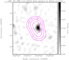
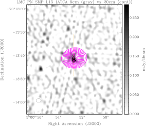
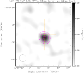
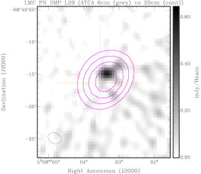
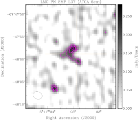
Figure 1: New and previous radio detections of LMC PNe. Images are constructed as total intensity radio maps. Contours are integral multiples of the measured RMS noise starting at 3$\sigma$ with spacings of 1$\sigma$. Top row: SMP L13 at 6 cm (grey scale) with 20 cm contours and SMP L15 at 6 cm (grey scale) with 20 cm contours; Second row: SMP L21 at 6 cm and SMP L23 at 13 cm (grey scale) with 20 cm contours; Third row: SMP L29 at 6 cm (grey scale) with 20 cm contours and SMP L37 at 6 cm. The beam size of each image is shown in the bottom left corner. The orange crosses represent the PN positions from the RP catalogue.

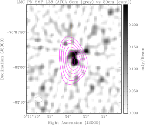
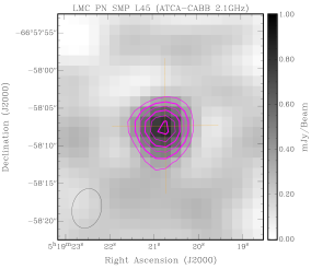
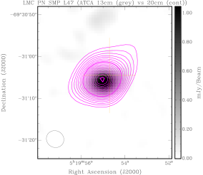
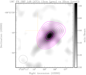
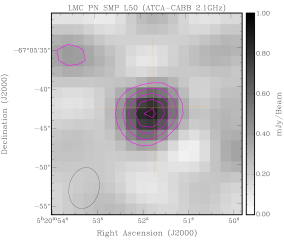
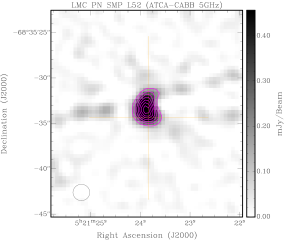
Figure 2: New and previous radio detections of LMC PNe. Images are constructed as total intensity radio maps. Contours are integral multiples of the measured RMS noise starting at 3$\sigma$ with spacings of 1$\sigma$. Top row: SMP L38 at 6 cm (grey scale) with 20 cm contours and SMP L45 at 2.1 GHz; Second row: SMP L47 and SMP 48 at 13 cm (grey scale) with 20 cm contour; Third row: SMP L50 at 2.1 GHz and SMP L52 at 5 GHz. The beam size of each image is shown in the bottom left corner. The orange crosses represent the PN positions from the RP catalogue.

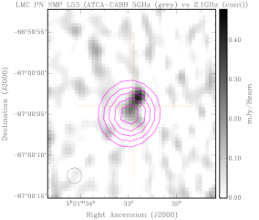
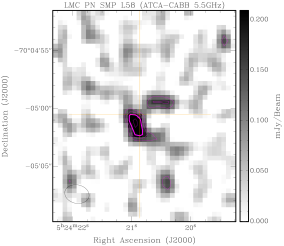
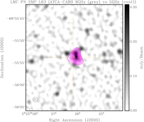
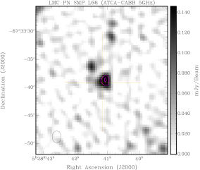
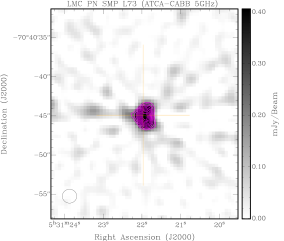
Figure 3: New and previous radio detections of LMC PNe. Images are constructed as total intensity radio maps. Contours are integral multiples of the measured RMS noise starting at 3$\sigma$ with spacings of 1$\sigma$. Top row: SMP L53 at 5 GHz (grey scale) with 2.1 GHz contours and SMP L58 at 5.5 GHz; Second row: SMP L62 at 3 cm (grey scale) with 6 cm contours and SMP L63 at 9 GHz (grey scale) with 5 GHz contours; Third row: SMP L66 at 5 GHz and SMP L73 at 5 GHz. The beam size of each image is shown in the bottom left corner. The orange crosses represent the PN positions from the RP catalogue.

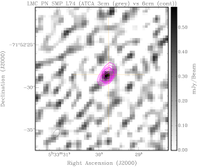
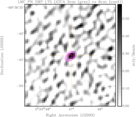
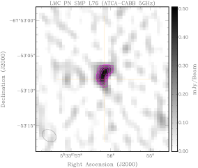
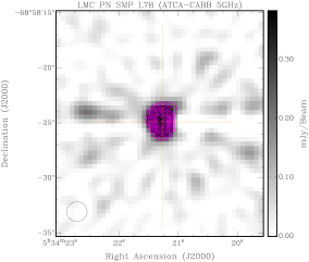
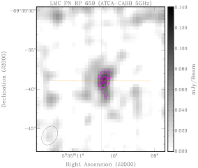
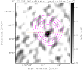
Figure 4: New and previous radio detections of LMC PNe. Images are constructed as total intensity radio maps. Contours are integral multiples of the measured RMS noise starting at 3$\sigma$ with spacings of 1$\sigma$. Top row: SMP L74 at 3 cm (grey scale) with 6 cm contours and SMP L75 at 3 cm (grey scale) with 6 cm contours; Second row: SMP L76 at 5 GHz and SMP L78 at 5 GHz; Third row: RP 659 at 5 GHz and SMP L83 at 6 cm (grey scale) with 20 cm contours. The beam size of each image is shown in the bottom left corner. The orange crosses represent the PN positions from the RP catalogue.

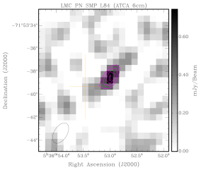
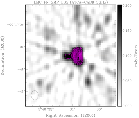
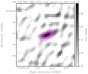
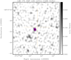
Figure 5: New and previous radio detections of LMC PNe. Images are constructed as total intensity radio maps. Contours are integral multiples of the measured RMS noise starting at 3$\sigma$ with spacings of 1$\sigma$. Top row: SMP L84 at 6 cm and SMP L85 at 5 GHz; Bottom row: SMP L89 at 3 cm (grey scale) with 6 cm contours and SMP L92 at 5 GHz. The beam size of each image is shown in the bottom left corner. The orange crosses represent the PN positions from the RP catalogue.

3.2 Detection Results

After careful examination of all of our available data, 21 new RC detections of PNe in our base catalogue were identified: SMP L13, SMP L15, SMP L21, SMP L23, SMP L29, SMP L37, SMP L38, SMP L45, SMP L50, SMP L52, SMP L53, SMP L58, SMP L63, SMP L66, SMP L73, SMP L75, SMP L76, SMP L78, RP 659, SMP L85, and SMP L92.

For seven previously detected PNe (Filipović et al., 2009): SMP L47, SMP L48, SMP L62, SMP L74, SMP L83, SMP L84, and SMP L89, a flux density was measured on at least one frequency, confirming previous detections. The data for these PN detections come from the various ATCA projects listed in Table 1. All of the RC LMC PNe detected here are from the set of PN coordinates that RP has published with a classification of ‘Known’ or ‘True’.

The four PNe listed in Filipović et al. (2009) for which we did not find any new reliable detections were SMP L8, SMP L25, SMP L33, and SMP L39. SMP L8 has been reclassified as a compact H ii region and is not listed in the RP catalogue. Therefore, they are not included in our study presented here. We detected RC emission from the positions of previously known RC PNe SMP L25 and SMP L33 in 20 cm data from ATCA project C354. Unfortunately, both PNe are far from the centre of the primary beam ($\sim$25 arcmin at 20 cm) and therefore their flux density measurements are very uncertain even after the image has been corrected for the primary beam (miriad linmos task). SMP L39 was not contained in any of the projects which met our requirements for inclusion.

The RP coordinates and the measured integrated radio flux densities for the detected PNe are shown in Table LABEL:tbl:MeasureRC. The flux densities of the three previously detected PNe which we could not measure, SMP L25, SMP L33, SMP L39, are included in Table LABEL:tbl:MeasureRC with intensities from Filipović et al. (2009) for completeness of the LMC PN sample. The finding charts for all LMC PN RC detections are shown in Figs. 1 through 5. These images are constructed as total intensity RC maps at the detection frequencies overlaid with contours at integral multiples of the estimated RMS noise. The orange crosses represent the PN coordinates from the RP catalogue.

As can be seen from the finding charts presented (Fig. 1–5), in most cases the radio detections are of isolated sources well correlated with their RP catalogue optical counterparts. Most detections of a PN were at one or two frequencies with only two detections at three frequencies and none at four frequencies. The absence of detection at more frequencies was due either to a lack of data for a PN at that frequency or that the emissions were determined to be below the 3$\sigma$ noise level.

Table 3: Coordinates and flux density measurements of detected LMC PNe. The new flux density measurements are shown in the columns titled ‘new’ and previous detections (Filipović et al., 2009) are listed in the columns titled ‘F09’. The symbol ‘$<$’ indicates that the actual value is less than the indicated value. Col. 12 is the MIR/S${}_{20\,cm}$ ratio using $8~{}\mu$m data from the VizieR Online Data Catalog: SAGE LMC and SMC IRAC Source Catalog (IPAC 2009). Col. 13 is the calculated H$\alpha$ flux using tabulated H$\beta$ and extinction values cH$\beta$ from (Reid & Parker, 2010). Col. 14 is from Table LABEL:tbl:physprop. The ‘Source Ref.’, Col 15, refers to the sources of the RC data used for our measurements from the ATCA project data base references found at the bottom of this table.

No.	PN	RA	DEC	S${}_{3\,cm}$ (mJy)		S${}_{6\,cm}$ (mJy)		S${}_{13\,cm}$ (mJy)		S${}_{20\,cm}$ (mJy)		MIR/	H$\alpha$ flux $(10^{-13})$	$\theta$	Source
		(J2000)	(J2000)	new	F09	new	F09	new	F09	new	F09	S${}_{20\,cm}$	${\text{erg c}}{{\text{m}}^{-2}}{\text{ }}{{\text{s}}^{-1}}$	(″)	Ref.
	(1)	(2)	(3)	(4)	(5)	(6)	(7)	(8)	(9)	(10)	(11)	(12)	(13)	(14)	(15)
1	SMP L13	04:59:59.99	–70:27:40.8	…	…	0.40$\pm$0.04	…	…	…	0.45$\pm$0.04	…	18.0	5.8	0.94	8
2	SMP L15	05:00:52.71	–70:13:41.1	…	…	0.64$\pm$0.05	…	0.98$\pm$0.05	…	0.90$\pm$0.06	…	24.4	6.5	0.82	4,8
3	SMP L21	05:04:51.99	–68:39:09.7	…	…	0.62$\pm$0.05	…	…	…	…	…	…	6.9	0.24	8
4	SMP L23	05:06:09.45	–67:45:27.8	…	…	…	…	0.67$\pm$0.04	…	0.66$\pm$0.04	…	4.4	6.7	0.39	5
5	SMP L25	05:06:23.91	–69:03:19.0	…	2.4$\pm$0.24	…	2.1 $\pm$0.21	…	…	…	1.8$\pm$0.2	10.5	14.7	0.46	…
6	SMP L29	05:08:03.32	–68:40:16.6	…	…	0.65$\pm$0.06	…	…	…	0.70$\pm$0.07	…	17.9	5.9	0.54	3,8
7	SMP L33	05:10:09.41	–68:29:54.5	…	1.8$\pm$0.2	…	$<$1.5	…	…	…	$<$1	…	5.1	0.62	…
8	SMP L37	05:11:02.92	–67:47:59.4	…	…	0.52$\pm$0.04	…	…	…	…	…	…	3.3	0.50	8
9	SMP L38	05:11:23.69	–70:01:57.4	…	…	0.58$\pm$0.05	…	…	…	0.58$\pm$0.05	…	87.9	7.0	0.50	6,8
10	SMP L39	05:11:42.11	–68:34:59.1	…	$<$1.5	…	$<$1.5	…	…	…	2.3 $\pm$0.23	3.0	2.2	0.46	…
11	SMP L45	05:19:20.71	–66:58:06.9	…	…	…	…	1.00$\pm$0.10	…	…	…	…	3.6	1.44	9
12	SMP L47	05:19:54.65	–69:31:05.1	…	2.3$\pm$0.23	…	2.1$\pm$0.21	1.50$\pm$0.05	…	1.30$\pm$0.05	2.2$\pm$0.22	17.1	11.3	0.50	1
13	SMP L48	05:20:09.48	–69:53:39.1	…	$<$1	1.4$\pm$0.2	1.5$\pm$0.2	1.50$\pm$0.10	…	1.00$\pm$0.05	1.6$\pm$0.2	18.0	10.2	0.40	1
14	SMP L50	05:20:51.73	–67:05:43.4	…	…	…	…	1.00$\pm$0.15	…	…	…	…	6.5	0.70	9
15	SMP L52	05:21:23.96	–68:35:33.8	…	…	1.00$\pm$0.05	…	…	…	…	…	…	11.1	0.40	8
16	SMP L53	05:21:32.83	–67:00:04.6	…	…	0.61$\pm$0.06	…	0.92$\pm$0.15	…	…	…	…	20.7	0.80	8,9
17	SMP L58	05:24:20.77	–70:05:01.5	…	…	0.31$\pm$0.05	..	…	…	…	…	…	9.0	0.26	8
18	SMP L62	05:24:55.08	–71:32:56.3	2.1$\pm$0.2	1.8$\pm$0.2	2.6$\pm$0.1	2.1$\pm$0.21	…	…	…	2.5 $\pm$0.3	3.0	18.8	0.54	2
19	SMP L63	05:25:26.02	–68:55:54.0	0.5$\pm$0.1	…	1.2$\pm$0.1	…	…	…	…	…	…	12.7	0.52	8
20	SMP L66	05:28:41.00	–67:33:39.3	…	…	0.25$\pm$0.05	…	…	…	…	…	…	8.3	1.08	8
21	SMP L73	05:31:21.89	–70:40:45.5	…	…	1.01$\pm$0.06	…	…	…	…	…	…	13.7	0.50	8
22	SMP L74	05:33:29.76	–71:52:28.5	0.97$\pm$0.15	$<$1.5	1.06$\pm$0.15	$<$1.5	…	…	…	3.0$\pm$0.3	5.2	…	0.70	8
23	SMP L75	05:33:47.00	–68:36:44.2	1.14$\pm$0.15	…	1.45$\pm$0.15	…	…	…	…	…	…	10.2	0.40	8
24	SMP L76	05:33:56.10	–67:53:09.2	…	…	0.61$\pm$0.07	…	…	…	…	…	…	13.7	…	8
25	SMP L78	05:34:21.19	–68:58:25.3	…	…	1.28$\pm$0.06	…	…	…	…	…	…	12.5	0.56	8
26	RP 659	05:35:10.19	–69 39 39.3	…	…	0.12$\pm$0.02	…	…	…	…	…	…	1.2	…	7
27	SMP L83	05:36:20.81	–67:18:07.5	…	0.7$\pm$0.07	0.74$\pm$0.10	0.9$\pm$0.1	…	…	0.9$\pm$0.1	1.6 $\pm$0.2	1.4	4.9	2.52	3
28	SMP L84	05:36:53.46	–71:53:39.3	…	$<$1.5	0.80$\pm$0.11	$<$1.5	…	…	…	1.6$\pm$0.2	1.7	…	0.58	8
29	SMP L85	05:40:30.80	–66:17:37.4	…	…	1.15$\pm$0.06	…	…	…	…	…	…	6.5	…	8
30	SMP L89	05:42:37.17	–70:09:30.4	1.60$\pm$0.15	1.8$\pm$0.2	1.49$\pm$0.10	1.6$\pm$0.2	…	…	…	2.1$\pm$0.21	13.3	7.9	0.46	8
31	SMP L92	05:47:04.80	–69:27:32.1	…	…	0.41$\pm$0.06	…	…	…	…	…	…	6.6	0.52	8

Table 4: Measured and calculated LMC PN RC parameters. Col. 2 contains the photometric angular diameters. The references used for the diameters are listed in Col. 3 and they refer to the list at the bottom of the table. The spectral indexes ($\alpha$) are listed in Col. 4a and 4b. The adopted flux densities at 6 cm are in Col. 5. Those which are in brackets were estimated from other band measurements. The angular diameters in Col. 2 in arcseconds are used to calculate the radii in pc shown in Col. 7. Values for brightness temperatures (T_b), the electron densities (n_e) and ionised masses (M_i) are calculated from the adopted 6 cm flux densities and the radii. These are presented in Cols. 6, 8, and 9, respectively.

PN	$\theta$	Ref	$\alpha$		S${}_{6\,cm}$	Tb	r	log($n_{e}$)	$M_{i}$
	(″)		$>$5 GHz	$<$ 5 GHz	(mJy)	(K)	(pc)	(cm-3)	($M_{\odot}$)
(1)	(2)	(3)	(4a)	(4b)	(5)	(6)	(7)	(8)	(9)
SMP L13	0.94	1	…	–0.09$\pm$0.10	0.40$\pm$0.04	25$\pm$3	0.11	3.19	0.225
SMP L15	0.82	1	…	–0.27$\pm$0.10	0.64$\pm$0.05	68$\pm$5	0.10	3.38	0.236
SMP L21	0.24	4	…	…	0.62$\pm$0.05	594$\pm$48	0.03	4.17	0.036
SMP L23	0.40	3	…	00.28$\pm$0.20	$[$0.68$\pm$0.04$]$	302$\pm$18	0.05	3.87	0.075
SMP L25	0.46	1	00.27$\pm$0.40	00.11$\pm$0.20	2.1$\pm$0.21	559$\pm$56	0.06	4.02	0.167
SMP L29	0.54	2	…	–0.05$\pm$0.13	0.65$\pm$0.06	124$\pm$11	0.07	3.65	0.128
SMP L33	0.62	1	…	…	$[$1.9$\pm$0.2$]$	339$\pm$36	0.07	3.80	0.252
SMP L37	0.50	2	…	…	0.52$\pm$0.04	116$\pm$9	0.06	3.66	0.096
SMP L38	0.50	1	…	00.00$\pm$0.13	0.58$\pm$0.05	130$\pm$11	0.06	3.68	0.103
SMP L39	0.46	2	…	…	$[$2.0$\pm$0.2$]$	645$\pm$65	0.06	4.00	0.168
SMP L45	1.44	2	…	…	$[$0.88$\pm$0.09$]$	29$\pm$3	0.17	3.09	0.612
SMP L47	0.50	2	…	00.26$\pm$0.13	2.1$\pm$0.21	493$\pm$49	0.06	3.96	0.203
SMP L48	0.40	2	…	00.22$\pm$0.08	1.4$\pm$0.2	596$\pm$85	0.05	4.02	0.116
SMP L50	0.70	1	…	…	$[$0.93$\pm$0.14$]$	128$\pm$19	0.08	3.56	0.216
SMP L52	0.40	2	…	…	1.0$\pm$0.05	349$\pm$17	0.05	3.94	0.096
SMP L53	0.80	1	…	–0.44$\pm$0.30	0.61$\pm$0.06	53$\pm$5	0.10	3.39	0.211
SMP L58	0.26	1	…	…	0.31$\pm$0.05	260$\pm$42	0.03	3.98	0.028
SMP L62	0.54	2	–0.43$\pm$0.30	…	2.6$\pm$0.1	496$\pm$19	0.07	3.95	0.251
SMP L63	0.52	2	–1.80$\pm$0.60	…	1.2$\pm$0.1	251$\pm$21	0.06	3.84	0.160
SMP L66	1.10	4	…	…	0.25$\pm$0.05	12$\pm$2	0.13	2.99	0.214
SMP L73	0.50	2	…	…	1.01$\pm$0.06	226$\pm$13	0.06	3.80	0.135
SMP L74	0.70	2	–0.18$\pm$0.60	…	1.06$\pm$0.15	121$\pm$17	0.08	3.59	0.236
SMP L75	0.40	2	–0.50$\pm$0.50	…	1.45$\pm$0.15	507$\pm$52	0.05	4.03	0.115
SMP L76	…	…	…	…	0.61$\pm$0.07	…	…	…	…
SMP L78	0.56	1	…	…	1.28$\pm$0.06	230$\pm$11	0.07	3.78	0.179
RP 659	…	…	…	…	0.12$\pm$0.02	…	….	….	…
SMP L83	2.53	2	…	–0.14$\pm$0.20	0.74$\pm$0.10	7$\pm$1	0.30	2.68	1.337
SMP L84	0.50	2	…	…	0.80$\pm$0.11	132$\pm$18	0.07	3.65	0.150
SMP L85	…	…	…	…	1.15$\pm$0.06	…	…	…	…
SMP L89	0.46	2	00.14$\pm$0.30	…	1.49$\pm$0.10	397$\pm$27	0.06	3.94	0.143
SMP L92	0.52	2	…	…	0.41$\pm$0.06	86$\pm$13	0.06	3.58	0.090

3.3 Radio-continuum properties of the detected PNe

From the measurements made here and data from the literature, additional physical properties of the detected PNe were determined. In Table LABEL:tbl:MeasureRC (Column 12) we calculated the ratio of Mid-Infrared (MIR) and 20 cm flux densities using $8~{}\mu$m MIR data from the Sage LMC and SMC IRAC Source Catalog (IPAC 2009) containing LMC data from Meixner et al. (2006). This data was downloaded from the VizieR Online Data Catalog collection. Cohen et al. (2007b) using Galactic data from Cohen & Green (2001) and other sources referenced therein, examined the MIR-RC ratio, ${{{S_{8.3\mu m}}}\mathord{\left/{\vphantom{{{S_{8.3\mu m}}}{{S_{843\,MHz}}}}}\right.\kern-1.2pt}{{S_{\rm 843\,MHz}}}}$ for PNe in the Galactic plane and calculated a median ratio of 12. The median ratio for our population of the LMC PNe is 11.9 using ${{{S_{8\mu m}}}\mathord{\left/{\vphantom{{{S_{8\,\mu m}}}{{S_{1.4\,GHz}}}}}\right.\kern-1.2pt}{{S_{\rm 1.4\,GHz}}}}$. The largest deviation from this median in our sample was calculated to be 87.9 for SMP L38. This, however, is likely to be due to unusual dust emissions from polycyclic aromatic hydrocarbons emitted by this PN as discussed in Bernard-Salas et al. (2009) who included this PN in their study of the MC PNe.

In Table LABEL:tbl:physprop, the RC spectral energy distribution (SED) was calculated for each PN for which measurements of flux density had been made on at least two frequencies. The fitting equation is:

$$S_{\nu}=\beta\nu^{\alpha}$$ (1)

where $\alpha$ is the spectral index and $S_{\nu}$ is the flux density at frequency $\nu$. The spectral indices are shown in Cols. 4a and 4b of Table LABEL:tbl:physprop.

PN RC emission is primarily thermal radiation from free-free interactions between electrons and ions within the nebular shell (Kwok, 2000). The SED is dependent on the metallicity, electron density, and temperature. Typically, at higher frequencies ($>$5 GHz), the nebula is optically thin and the spectral index ($\alpha$) is expected to be $\sim-0.1$. At lower frequencies ($<$5 GHz), young PNe are most likely optically thick with an expected spectral index of $\sim$2 (Pottasch, 1984). However, different density profile models can produce a very different SED. For example, if the density profile is from a constant mass loss, the spectral index for the PN would be optically thin and observed to be inverted with $\alpha\sim$0.6 (Panagia & Felli, 1975). Gruenwald & Aleman (2007) cautions that radio SED observations from PNe cannot uniquely determine the density profiles of the PNe.

The critical frequency of a PN is defined as the transition frequency from optically thick with a positive spectral index to optically thin with a negative spectral index. Most Galactic PNe exhibit a critical frequency of less than 5 GHz (Gruenwald & Aleman, 2007). However, the critical frequencies for the PNe depend on gas density and can range from $\sim$0.4 GHz to $>$15 GHz (Gruenwald & Aleman, 2007). Young and compact PNe have been observed with critical frequencies of $\sim$5 GHz to 28 GHz (Aaquist & Kwok, 1991). These young PNe most likely have very high electron densities which makes the critical frequency much higher than 5 GHz (Kwok, 1982; Pazderska et al., 2009). We calculated the spectral indices $\alpha$ above and below 5 GHz from Eq. 1 as a proxy of the evolutionary state of the PNe.

Non-thermal radio emission has been proposed for some PN emissions (Dgani & Soker, 1998). The mechanism offered requires fast winds from the CS of the PN to create an inner region where strong magnetic fields are interacting with the CS wind. A non-thermal SED would be expected to have a spectral index $\alpha\ll-0.1$ (Gurzadyan, 1997). Cohen et al. (2006) reported non-thermal emissions from a very unusual Asymptotic Giant Branch (AGB) star. This star was measured to have $\alpha\sim-0.9$ and contained shocked interactions between a cold PN–like nebular shell and the hot, fast stellar wind from the AGB star. The source, however, of most apparent non-thermal radio detections is more likely to be a Supernova Remnant or an Active Galactic Nucleus coincident with the position of the PN.

In Col. 5 (Table LABEL:tbl:physprop) the adopted flux densities at 6 cm for all of the detected RC PNe are presented. If direct measurement at 6 cm was not available, we estimated the flux density from neighbouring bands. This was necessary for SMP L23, SMP L33, SMP L39, and SMP L45. The entries that are estimated are indicated in Table LABEL:tbl:physprop with brackets around the 6 cm values.

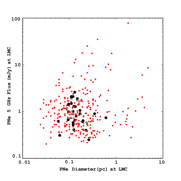
Figure 6: Galactic PNe from (Siódmiak & Tylenda, 2001) (small red dots), SMC PNe data from (Leverenz et al., 2016) (green stars), (both scaled to the distance of the LMC), and our new LMC measurements (large black dots).

We also compared our adopted 6 cm flux densities with a sample of well-measured Galactic PNe (GPNe). This sample is a data base of optical diameters and 6 cm integrated flux density measurements from Siódmiak & Tylenda (2001) consisting primarily of PNe from the Galactic bulge. Their diameter measurements were calculated using the 10 per cent peak contour approach. They used only optical data from photographic plates since they judged that newer CCD images were too sensitive and could not be directly compared to extant diameter measurements derived from photographic plates. We re-scaled their data to the distance of the LMC (50 kpc; Pietrzyński et al. (2013)) and plotted both data-sets on the same figure (Fig. 6). Additionally we included nine SMC PNe from Leverenz et al. (2016): SMP S6, SMP S13, SMP S14, SMP S16, SMP S17, SMP S18, SMP S19, SMP S22, and SMP S24. These SMC PNe were unambiguously determined not to be PN mimics and were also re-scaled to the distance of the LMC. The green star markers on Fig. 6 represent the SMC data.

Our RC LMC PN measurements are consistent with the scaled flux densities and diameters from both the Galactic and SMC samples. The angular diameters in Table LABEL:tbl:physprop (Col. 2) were adopted from Shaw et al. (2001, 2006), Vassiliadis et al. (1998), and Stanghellini et al. (1999). For consistency, we chose only photometric radii defined as the radius containing 85 per cent of the total emitted flux (Shaw et al., 2001) since measurements based on this method were available from all of the sources we consulted for the radius data which we adopted. We estimated that the differences in the techniques for the diameter measurements for this comparison was not significant (the 10 per cent peak flux density used by Siódmiak & Tylenda (2001) for the GPNe compared to the 85 per cent flux density limit we employed for the MC PNe).

We used our adopted 6 cm flux densities and the angular diameters from the literature to estimate the electron densities ($n_{e}$) and ionized masses ($M_{i}$) for all detected RC PNe (Table LABEL:tbl:physprop, Cols. 8 and 9). The $n_{e}$ and $M_{i}$ are calculated from equations (1) and (2) in Gathier (1987), respectively. The electron temperature ($T_{e}$) for all PNe was chosen to be the canonical temperature of 10 000 K. The solar metallicity parameter and the consensus filling factors were both assigned a numerical value of $0.3$ (Boffi & Stanghellini, 1994; Frew et al., 2016a). The helium abundance for SMP L13 was taken from de Freitas Pacheco et al. (1993). SMP L39, SMP L52, and RP 659 were assigned the default value of 0.1 per Gathier (1987) since measured values for those PNe were not available. Calculations for the remaining PNe used helium abundances from Chiappini et al. (2009). No values for the fraction of doubly ionised helium were available so we adopted the default value of $1/3$ as used by Gathier (1987). Uncertainties in $n_{e}$ and $M_{i}$ are estimated to be on the order of 40 per cent.

Thermal brightness (T_b) at 6 cm is shown in Table LABEL:tbl:physprop (Col. 6). It is a good proxy for PN evolutionary status (Kwok, 1985; Zijlstra, 1990; Gruenwald & Aleman, 2007) and also an indication of self absorption. We calculated the conventional radio thermal brightness assuming an isothermal nebula from Wilson et al. (2009) as follows:

$${T_{b}}=\frac{{{c^{2}}}}{{2k{\nu^{2}}}}\cdot\frac{{{S_{\nu}}}}{{\Delta\Omega}}$$ (2)

To determine the self absorption correction for our results, we applied the two component model of self absorption from Siódmiak & Tylenda (2001). We adopted the values of $\xi=0.27$ and $\varepsilon=0.19$ for this comparison. This model provides a correction factor based on the ratio of the measured $T_{b}$ with the electron temperature, $T_{e}$. We adopted the canonical value of 10000 K for $T_{e}$. The highest thermal brightness we calculated from our data is from SMP L39 at 645 K. For this value of $T_{b}$, the model gives a correction factor of 1.8 at 20 cm and 1.01 at 6 cm. The value of 339 K for $T_{b}$ from SMP L33 is determined to have a correction factor of 1.4 at 20 cm. At 6 cm, there is essentially no self absorption. Our conclusion was that there was significant self absorption in some of our results at 20 cm but at shorter wavelengths the self absorption was negligible.

4 $\Sigma-D$ relation for PNe

Table 5: Results of the $\Sigma$–$D$ analysis at 6 cm. Col. 1 lists the sample designation with the number of data points in Col. 2 and the calculated correlation coefficient in Col. 3. Cols. 4-7 list the values for the parameters of the fitting from the $\Sigma$ offsets and their estimated uncertainties. The average fractional error for the calculated distances are in Col. 8. Cols. 9-13 present the values for the orthogonal-offset-fitting and the corresponding average distance fractional errors. In Cols. 14-16 we present the average fractional errors for the PDF distance estimators: mean, mode, and median.

Sample			$\Sigma$ offsets						Orthogonal offsets						$f(\%)$
	$N$	$r$	$A$	$\Delta A$	$\beta$	$\Delta\beta$	$f(\%)$		$A$	$\Delta A$	$\beta$	$\Delta\beta$	$f(\%)$		mean	mode	median
(1)	(2)	(3)	(4)	(5)	(6)	(7)	(8)		(9)	(10)	(11)	(12)	(13)		(14)	(15)	(16)
LMC	28	–0.87	–19.7	0.3	2.2	0.4	22.97		–20.3	0.4	2.9	0.5	19.58		18.29	17.28	18.37
SMC†	9	–0.94	–20.1	…	2.7	…	9.99		–20.4	…	3.0	…	9.52		…	…	…
LMC+SMC	37	–0.88	–19.9	0.3	2.3	0.3	20.17		–20.3	0.3	2.9	0.4	17.00		16.05	14.64	16.02

^† Presented results are not reliable due to the small number of data points and are given only for the sake of completeness. Unlike the other two samples, these fitting parameters are not determined with the bootstrap procedure described in the paper but from a simple linear regression fitting to the data sample. The 2D density smoothing did not yield convergent results and no fractional errors were calculated.

The radio flux measurements at 6 cm and radius measurements in parsecs from Table LABEL:tbl:physprop were used to calculate the surface brightness and diameter values for the $\Sigma$–$D$ relation study of the MC PNe.

Recently, Leverenz et al. (2016) described the $\Sigma$–$D$ relation for a sample of SMC PNe. Here, we extended that work by analyzing our radio detected PNe in terms of the $\Sigma$–$D$ relation for both the LMC and the SMC. The model for the radio surface brightness we adopted from Vukotić et al. (2009) is shown in the following equation:

$$\Sigma\left[{\text{W}}{{\text{m}}^{-2}}{\text{H}}{{\text{z}}^{-1}}{\text{s}}{{\text{r}}^{-1}}\right]=1.505\cdot{10^{-19}}{{S\left[\text{Jy}\right]}\mathord{\left/{\vphantom{{S\left[{Jy}\right]}{{\theta^{2}}\left[{}^{\prime}\right]}}}\right.\kern-1.2pt}{{\theta^{2}}\left[\arcmin\right]}}$$ (3)

The form of the $\Sigma$–$D$ model equation adopted for these surface brightness calculations is

$$\Sigma=AD^{-\beta}$$ (4)

see Vukotić et al. (2014).

There are 715 observed PNe in the LMC (Reid & Parker, 2013; Reid, 2014) but only 31 of them have been detected at radio frequencies. This is indicative of a strong observational bias suggesting that only the ‘tip of the iceberg’ is observed at radio frequencies, see Vukotić et al. (2009). Indeed, while the measured surface brightness of GPNe extends from $\sim 10^{-24}$ to $\sim 10^{-16}$ ${\text{W}}{{\text{m}}^{-2}}{\text{H}}{{\text{z}}^{-1}}{\text{s}}{{\text{r}}^{-1}}$ , the PNe from the MCs are detected only in the high brightness half of this interval from $\sim 10^{-20}$ to $\sim 10^{-16}$ ${\text{W}}{{\text{m}}^{-2}}{\text{H}}{{\text{z}}^{-1}}{\text{s}}{{\text{r}}^{-1}}$. Similar selection effects can be seen in $D$ as well. The largest PN in our radio LMC sample is smaller than 1 pc, unlike the largest PN used for H$\alpha$ statistical distance calibration (Frew et al., 2016a) being $>2$ pc in size.

With such a strong selection effect in play we constructed a Monte Carlo simulation (described in Section 4.4) to quantify the influence of sensitivity related selection effects on our $\Sigma$–$D$ samples. We utilised bootstrap statistics (Efron & Tibshirani, 1993) to reconstruct the prior distribution of the $\Sigma$–$D$ relation parameters. For each $\Sigma$–$D$ data sample we applied both $\Sigma$ offset and orthogonal offset analysis. In addition, we reconstructed the $\Sigma$–$D$ probability density function (PDF) using bootstrap based kernel density smoothing (for details see Bozzetto et al., 2017, and references therein). The reconstruction of the $\Sigma$–$D$ PDF provides a better insight into observational biases and evolutionary features of each sample (see also Vukotić et al., 2014, and references therein). Unlike Vukotić et al. (2014), the PDF calculation is improved with the use of bootstrap based kernel density smoothing instead of bootstrap based centroid offset smoothing. We applied a standard Gaussian kernel in order to calculate optimal smoothing bandwidths. For data in two dimensions a Gaussian product kernel was used. The optimal smoothing bandwidths ($h$) were selected by minimising the bootstrap integrated mean squared error (BIMSE) (for details see Bozzetto et al., 2017).

From the LMC and SMC data we defined three samples: 1) the sample of 28 LMC PNe; 2) the sample of 9 SMC PNe with reliable flux density estimates; 3) the sample consisting of the combined LMC + SMC PNe with 37 total PNe.

As a measure of the sample spread and reliability we calculated the correlation coefficient $r$ and the average fractional error $f$. For the $\Sigma$–$D$ statistical distances to the MCs, we calculated $f$ and estimated the distances from the $\Sigma$–$D$ relation (for a detailed description of statistical distance calculation see Vukotić et al. (2014)). The results are shown in Table 5 and Fig. 7.

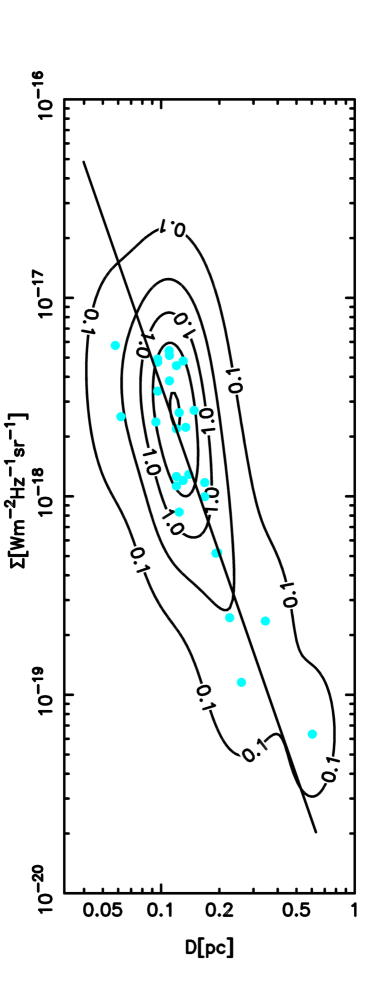
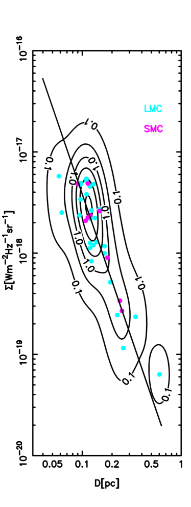
Figure 7: $\Sigma$–$D$ data plots at 6 cm with the reconstructed data probability density distribution and orthogonal regression best-fitting line: LMC (left) and LMC+SMC (right). The PDF contour plot is calculated on the $100\times 100$ grid mapped on the plotted variables range. Contours levels are at 0.1, 0.5, 1.0, 1.5, 2.0 and 2.5. Optimal smoothing bandwidths are found at $h_{\log D}=0.11$ and $h_{\log\Sigma}=0.30$ for the LMC sample and $h_{\log D}=0.09$ and $h_{\log\Sigma}=0.26$ for the LMC+SMC sample.

The average fractional error for distance was calculated as:

$${f}=\frac{1}{N}\sum_{i=1}^{N}\left|\frac{d_{\mathrm{i}}-d_{\mathrm{i}}^{\mathrm{s}}}{d_{\mathrm{i}}}\right|$$ (5)

where $N$ is the number of data points in the sample, $d_{\mathrm{i}}$ is the measured distance to the object of the $\mathrm{i}^{\mathrm{th}}$ data point, and $d_{\mathrm{i}}^{\mathrm{s}}$ is a statistical distance to that object determined either from the parameters of an empirical fitting or from the PDF method. The PDF method for a fixed $\Sigma$ value gives a probability density over $D$. The values of $D$ for the mean, mode, and median are used to calculate the corresponding statistical distances (Table 5).

4.1 SMC sample

With the highest $r$ value and the smallest values for $f$ (Table 5) the SMC sample appears to be very compact and reliable. However, the kernel density smoothing does not give convergent results for optimal smoothing bandwidths. This is caused by the small number of data points. The optimal smoothing bandwidths are calculated around $\sim 0.14$ and $\sim 0.40$ but repeated calculations do not give consistent results.

We note that the SMC sample consists of a small number of data points that are difficult to measure accurately in that they are very close to the survey sensitivity line. This suggests that the quality of this sample could be weaker than it would first appear from a simple linear regression. Applying the bootstrap procedure could provide erroneous values for $A$ and $\beta$ and their uncertainties. The small number of data points, even with the high correlation value, gives non-physical values for $A$ and $\beta$ when fitting the re-sampled samples. This resampling with repetition is the essence of the bootstrap analysis (see Vukotić et al. (2014) and references therein).

Instead of presenting these erroneous values, in Table 5 we show values from a simple empirical fitting of a single line to the SMC sample without the application of the bootstrap analysis. Even though we do not consider these fitted parameter values reliable we do utilise the SMC sample to form a more complete combined MC PN sample.

4.2 LMC and combined sample

The larger LMC sample appears to be more complete and reliable than the SMC sample although it is also very close to the survey sensitivity line (Figs. 7 and 9). An interesting feature of these plots is that the data density contours in the $\Sigma-D$ plane at $\gtrsim 1$ levels are symmetric about the line of the steeper slope than the slope of the orthogonal offset best-fitting line for both LMC and the combined sample. This (a)symmetric discrepancy is evident over a large part of the plotted variables range, $D\lesssim 0.3$ pc. This is in agreement with the fig. 5 plot from Frew et al. (2016b) where the authors plotted similar quantities (H$\alpha$ brightness verses radius) along with the evolutionary paths for PNe of different masses. The plotted paths significantly deviate from a straight line in the $D\lesssim 0.3$ pc range. This reveals the need for developing new statistical tools for future empirical studies of PN evolution in order to quantify the subtleties of that evolution. With the larger data spread, the LMC sample is certainly less sensitivity biased than the SMC sample but the somewhat large uncertainties, especially $\Delta\beta\sim 0.4-0.5$, indicate a possible reduced sample quality. Although less extreme than the SMC sample, the LMC sample bias could cause peculiar values for the fitting of the parameters for the re-sampled sample.

Combining the SMC and LMC samples into one sample yielded the best results. The combined sample has smaller values for $\Delta A$ and $\Delta\beta$ compared to the LMC sample alone (Table 5). We also found that the average fractional distance error calculated with the PDF method for the combined sample is $f\sim 16$ per cent which is lower than that of the LMC sample alone which is $f\sim 18$ per cent. This demonstrates the potential of RC MC PN samples to be used for statistical distance estimates. However, $\sim 18$ per cent of the LMC’s $50$ kpc distance is $\sim$9 kpc. Comparing this to a 1 kpc LMC depth (Pietrzyński et al., 2013), (Frew et al., 2016c) suggests that there is still significant room for improvement. This is likely to be achieved by more sensitive and more accurate radio surveys with larger samples.

4.3 $\Sigma$–$D$ slope

The value of $\beta$ in the $\Sigma$–$D$ relation is theoretically expected to change from $\sim$1 to 3 over the lifetimes of the PNe (Urošević et al., 2009). Using a GPN sample they found an empirical slope of $\beta\simeq 2.3\pm 0.4$ by fitting the $\Sigma$ offsets. The $\beta$ values from $\Sigma$ offsets in this work, $2.3$ for combined sample and $2.2$ for the LMC sample alone, may imply a similar age for the MC PN population compared to their selected GPN sample. However, the more robust orthogonal slope of $2.9$ (Table 5) could give the impression that the MC PNe might be in a late stage of their evolution. Vukotić et al. (2009) argued that the MC PN samples are biased with sensitivity selection effects and consequently the empirical slopes should be steeper than that estimated from the $\Sigma-D$ empirical data fittings. Applying the bootstrap procedure to a sample of GPNe with reliable distances, Vukotić & Urošević (2012) obtained an orthogonal offset $\beta=3.1\pm 0.4$ which is consistent with our MC results presented in Table 5. Both the $\Sigma$ offset slope for the GPN sample from Urošević et al. (2009) and the orthogonal offset slope from Vukotić & Urošević (2012) overlap within the estimated uncertainties of the slopes from Table 5.

4.4 $\Sigma$–$D$ sensitivity selection effects

To estimate the accuracy of our results related to the $\Sigma$–$D$ slope we simulated the influence of sensitivity related selection effects. This method is from Vukotić et al. (2009) who applied this technique to a very small sample of five PNe. We performed a similar simulation (although more advanced in some technical details) applying this method to our MC PN samples. This great improvement in the number of radio MC PN detections should result in a significantly more complete PN sample.

To estimate the influence of the sensitivity selection effects we generated artificial PN $\Sigma$–$D$ samples using a Monte Carlo simulation from the properties of our 6 cm data and compared the sample parameters before and after sensitivity selection. With the smallest PN in our 6 cm sample having a diameter of $D_{\mathrm{min}}=0.058$ pc (Table LABEL:tbl:physprop) and the fact that the largest PNe usually swell up to $D_{\mathrm{max}}\sim 2$ pc, we distributed artificial points randomly generated in the $[D_{\mathrm{min}},D_{\mathrm{max}}]$ interval using the random number generator of Saito & Matsumoto (2008) with a uniform density on the $\log D$ scale equal to the density of the adopted 6 cm data. This resulted in a total of 55 artificial points (for the combined sample and 42 for the LMC sample) per generated sample in a given $[\log D_{\mathrm{min}},\log D_{\mathrm{max}}]$ interval. These points were then projected on to a series of lines with $\beta$ ranging from $1.5$ to $3.6$. All of these lines intersected the orthogonal offset best-fitting line to the 6 cm adopted data ($L_{\mathrm{o}}$) at $D_{\mathrm{min}}$. The next step was to disperse the points from the lines upon which they were projected in such a way as to simulate the dispersion of the adopted 6 cm data. This was achieved by applying the kernel density smoothing in 1D from Bozzetto et al. (2017). From the adopted 6 cm data we reconstructed the smooth probability density distribution of the orthogonal distances (offsets) from the $L_{\mathrm{o}}$ line (Fig. 8).

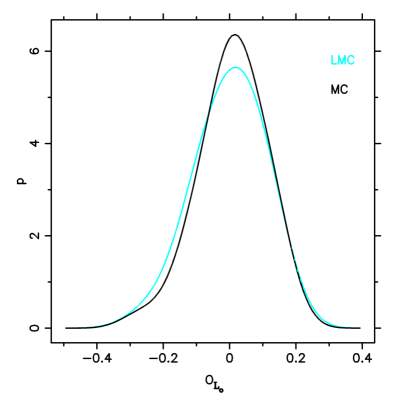
Figure 8: Our initial findings for the 6 cm data sample probability density distributions of the orthogonal distances from the orthogonal offset best-fitting lines $L_{\mathrm{o}}$ for the LMC and the combined sample.

It is reasonable to assume that the data do not have the same scatter along the simulated interval. We used empirical data for the input of our sensitivity simulation and we modeled the sensitivity line in such a way that it passed through the data point that gave the lowest $\Sigma$ value. We have no empirical knowledge of the data spread at the faint end. Even for the part above the sensitivity line, the PDF contours from Fig. 7 do not appear to have much variability in spread. In this way we simulated the uniform dispersion model for the whole simulated data interval. This is sufficient to demonstrate the influence of the sensitivity selection on the $\Sigma$–$D$ slope. Even if we use a different Scatter value at the faint end, most of it will get a sensitivity cut off and will not influence the results. Our initial findings (Fig. 8) showed no significant difference for the overall scatter in the case of the LMC and the combined sample. Both distributions were rather symmetric around the peak which was close to a value of zero. Each point was randomly dispersed in the orthogonal direction from the simulated slope line according to the probability density distribution from Fig. 8. The dispersion was controlled with a parameter called $Scatter$ which is multiplied by the dispersion obtained from the distributions in Fig. 8 to obtain the actual dispersion. We then calculated the orthogonal offset fitting parameters for the dispersed artificial sample. For each simulated slope we generated $100$ artificial samples. The mean values of the fitting parameters after selection and their estimated uncertainties (calculated as the standard deviation of the given array of elements) are presented in Table 6. In Fig. 9 we plotted one artificial sample for $Scatter=2.0$ with a simulated $\beta$ of $3.5$ along with the combined MC PN sample and sensitivity line. Since the presented LMC survey is not uniform in terms of sensitivity we selected the sensitivity line in such a way that it passed through the data point of the combined sample that gives the lowest $\Sigma$ value at the horizontal part of the sensitivity line. For the break point of the sensitivity line we selected the average equivalent of the circular beam size calculated from the beam sizes of each particular reduced image. At the adopted LMC distance this translates to $D=1.017$ pc.

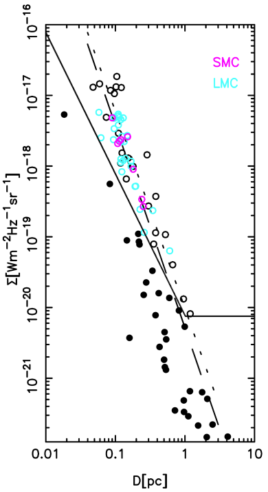
Figure 9: An example of an artificial sample generated from the combined sample orthogonal offsets for the simulated $\beta$ of $3.5$ and a $Scatter$ of 2.0. After selection the slope flattens to $2.8$ (short-dashed line fit). The solid line is the sensitivity line with the horizontal part at $\Sigma=7.54\times 10^{-21}$Wm^-2Hz^-1sr^-1 with the break point at $D=1.017$ pc. The long-dashed line is the orthogonal offset best-fitting to the combined MC PN sample. Data points in black are the simulated sample with the points below the sensitivity line plotted as filled circles.

Table 6: Parameters of the simulated samples and results of the sensitivity simulations for the LMC sample and the combined sample. Cols. 1-2 are the parameters from Equation 4 of the simulated $\Sigma$–$D$ evolution lines. While Cols. 3-7 present the results for LMC sample, Cols. 8-12 in a same way present the results for the combined sample. In Cols. 3 and 5 are the mean values of $\Sigma$–$D$ parameters calculated from the orthogonal offset fits after the selection has been applied and their estimated uncertainties are in Cols.  4 and 6, respectfully. In Col. 7 we give the difference between the mean slope after selection and the simulated slope. For all simulated slopes we fit 100 artificially generated samples.

			LMC sample						Combined sample
Simulated			After selection						After selection
$\log A$	$\beta$		$<\log A>$	$\sigma_{<\log A>}$	$<\beta>$	$\sigma_{<\beta>}$	$\Delta\beta$		$<\log A>$	$\sigma_{<\log A>}$	$<\beta>$	$\sigma_{<\beta>}$	$\Delta\beta$
(1)	(2)		(3)	(4)	(5)	(6)	(7)		(8)	(9)	(10)	(11)	(12)
$Scatter$ = 1.0
-18.62	1.50		-18.63	0.049	1.49	0.080	0.01		-18.56	0.035	1.48	0.054	0.02
-18.74	1.60		-18.75	0.054	1.59	0.083	0.01		-18.70	0.033	1.59	0.053	0.01
-18.87	1.70		-18.87	0.053	1.68	0.077	0.02		-18.82	0.037	1.69	0.060	0.01
-18.99	1.80		-19.00	0.057	1.79	0.093	0.01		-18.94	0.040	1.79	0.065	0.01
-19.11	1.90		-19.12	0.054	1.90	0.089	0.00		-19.07	0.045	1.89	0.062	0.01
-19.24	2.00		-19.24	0.070	2.00	0.112	0.00		-19.19	0.048	1.98	0.069	0.02
-19.36	2.10		-19.36	0.057	2.09	0.098	0.01		-19.31	0.049	2.09	0.075	0.01
-19.48	2.20		-19.48	0.064	2.20	0.107	-0.00		-19.44	0.048	2.19	0.071	0.01
-19.61	2.30		-19.59	0.061	2.26	0.098	0.04		-19.55	0.051	2.27	0.076	0.03
-19.73	2.40		-19.68	0.065	2.35	0.116	0.05		-19.66	0.049	2.36	0.084	0.04
-19.86	2.50		-19.78	0.078	2.40	0.120	0.10		-19.76	0.064	2.44	0.099	0.06
-19.98	2.60		-19.86	0.077	2.46	0.120	0.14		-19.85	0.063	2.50	0.102	0.10
-20.10	2.70		-19.94	0.097	2.53	0.159	0.17		-19.93	0.066	2.56	0.107	0.14
-20.23	2.80		-20.00	0.102	2.53	0.152	0.27		-20.01	0.075	2.61	0.110	0.19
-20.35	2.90		-20.07	0.136	2.61	0.167	0.29		-20.09	0.089	2.68	0.127	0.22
-20.47	3.00		-20.17	0.163	2.71	0.227	0.29		-20.16	0.099	2.72	0.132	0.28
-20.60	3.10		-20.18	0.144	2.71	0.197	0.39		-20.22	0.137	2.78	0.176	0.32
-20.72	3.20		-20.27	0.183	2.77	0.244	0.43		-20.28	0.128	2.81	0.168	0.39
-20.85	3.30		-20.32	0.262	2.79	0.323	0.51		-20.39	0.183	2.91	0.219	0.39
-20.97	3.40		-20.37	0.224	2.84	0.277	0.56		-20.45	0.169	2.96	0.209	0.44
-21.09	3.50		-20.46	0.433	2.92	0.444	0.58		-20.58	0.294	3.05	0.338	0.45
-21.22	3.60		-20.55	0.392	3.00	0.413	0.60		-20.61	0.281	3.08	0.308	0.52
$Scatter$ = 2.0
-18.62	1.50		-18.62	0.091	1.50	0.144	-0.00		-18.56	0.069	1.48	0.115	0.02
-18.74	1.60		-18.73	0.099	1.59	0.145	0.01		-18.70	0.074	1.60	0.123	0.00
-18.87	1.70		-18.87	0.107	1.71	0.182	-0.01		-18.80	0.077	1.68	0.115	0.02
-18.99	1.80		-18.96	0.095	1.80	0.153	-0.00		-18.92	0.065	1.77	0.105	0.03
-19.11	1.90		-19.09	0.101	1.90	0.165	0.00		-19.05	0.082	1.88	0.131	0.02
-19.24	2.00		-19.17	0.099	1.97	0.146	0.03		-19.17	0.083	1.99	0.125	0.01
-19.36	2.10		-19.29	0.100	2.09	0.151	0.01		-19.27	0.075	2.08	0.136	0.02
-19.48	2.20		-19.34	0.116	2.10	0.198	0.10		-19.36	0.084	2.14	0.141	0.06
-19.61	2.30		-19.42	0.111	2.17	0.173	0.13		-19.43	0.073	2.18	0.122	0.12
-19.73	2.40		-19.48	0.137	2.20	0.215	0.20		-19.52	0.078	2.26	0.129	0.14
-19.86	2.50		-19.56	0.129	2.29	0.212	0.21		-19.59	0.101	2.33	0.174	0.17
-19.98	2.60		-19.62	0.140	2.30	0.223	0.30		-19.66	0.106	2.36	0.182	0.24
-20.10	2.70		-19.68	0.145	2.37	0.225	0.33		-19.72	0.110	2.42	0.184	0.28
-20.23	2.80		-19.74	0.166	2.44	0.237	0.36		-19.80	0.129	2.48	0.196	0.32
-20.35	2.90		-19.77	0.156	2.46	0.259	0.44		-19.84	0.142	2.50	0.210	0.40
-20.47	3.00		-19.79	0.184	2.45	0.321	0.55		-19.88	0.169	2.53	0.230	0.47
-20.60	3.10		-19.85	0.198	2.48	0.278	0.62		-19.95	0.141	2.60	0.193	0.50
-20.72	3.20		-19.90	0.216	2.54	0.311	0.66		-19.97	0.180	2.58	0.252	0.62
-20.85	3.30		-19.95	0.227	2.59	0.329	0.71		-20.02	0.226	2.62	0.308	0.68
-20.97	3.40		-20.02	0.302	2.67	0.440	0.73		-20.01	0.212	2.62	0.260	0.78
-21.09	3.50		-20.09	0.397	2.72	0.541	0.78		-20.10	0.290	2.71	0.388	0.79
-21.22	3.60		-20.06	0.343	2.65	0.479	0.95		-20.18	0.290	2.79	0.346	0.81
$Scatter$ = 3.0
-18.62	1.50		-18.54	0.127	1.49	0.233	0.01		-18.51	0.091	1.47	0.167	0.03
-18.74	1.60		-18.67	0.129	1.59	0.217	0.01		-18.66	0.119	1.60	0.187	-0.00
-18.87	1.70		-18.78	0.135	1.72	0.243	-0.02		-18.76	0.104	1.70	0.173	-0.00
-18.99	1.80		-18.86	0.149	1.78	0.254	0.02		-18.88	0.105	1.81	0.182	-0.01
-19.11	1.90		-18.98	0.137	1.92	0.233	-0.02		-18.96	0.119	1.87	0.209	0.03
-19.24	2.00		-19.07	0.128	1.99	0.206	0.01		-19.06	0.105	1.97	0.169	0.03
-19.36	2.10		-19.14	0.158	2.01	0.298	0.09		-19.18	0.122	2.10	0.176	-0.00
-19.48	2.20		-19.18	0.130	2.07	0.191	0.13		-19.25	0.102	2.14	0.170	0.06
-19.61	2.30		-19.22	0.137	2.08	0.230	0.22		-19.31	0.116	2.19	0.208	0.11
-19.73	2.40		-19.30	0.153	2.21	0.287	0.19		-19.36	0.128	2.25	0.199	0.15
-19.86	2.50		-19.35	0.165	2.25	0.280	0.25		-19.43	0.130	2.24	0.214	0.26
-19.98	2.60		-19.37	0.159	2.26	0.338	0.34		-19.47	0.131	2.28	0.249	0.32
-20.10	2.70		-19.44	0.198	2.35	0.378	0.35		-19.53	0.132	2.35	0.210	0.35
-20.23	2.80		-19.51	0.190	2.35	0.357	0.45		-19.56	0.145	2.36	0.234	0.44
-20.35	2.90		-19.55	0.221	2.44	0.394	0.46		-19.58	0.156	2.37	0.246	0.53
-20.47	3.00		-19.57	0.266	2.41	0.448	0.59		-19.66	0.184	2.47	0.273	0.53
-20.60	3.10		-19.57	0.251	2.40	0.438	0.70		-19.70	0.166	2.49	0.286	0.61
-20.72	3.20		-19.69	0.266	2.58	0.438	0.62		-19.72	0.204	2.51	0.317	0.69
-20.85	3.30		-19.66	0.244	2.46	0.433	0.84		-19.78	0.283	2.58	0.410	0.72
-20.97	3.40		-19.71	0.310	2.60	0.529	0.80		-19.78	0.203	2.52	0.328	0.88
-21.09	3.50		-19.73	0.275	2.59	0.499	0.91		-19.83	0.250	2.58	0.382	0.92
-21.22	3.60		-19.76	0.313	2.60	0.493	1.00		-19.87	0.326	2.63	0.504	0.97

The results in Table 6 do not appear to be significantly dependent on $Scatter$. For each given $Scatter$ the $\Delta\beta$ becomes larger than $\sigma_{<\beta>}$ when the simulated $\beta$ becomes as large as $\sim 2.5-2.7$. This corresponds to $<\beta>\sim 2.5$ ($Scatter=1.0$) and, although within the estimated uncertainty, reduces to $<\beta>\sim 2.3$ for a larger $Scatter$. Hence the steeper slopes, such as $\sim 2.9$ (as obtained in this work) are significantly influenced by the sensitivity selection effect. For $<\beta>\sim 2.9$ the simulated slope is $\sim 3.4$ and is even greater for larger $Scatter$. Since the MC PN samples appear to be significantly influenced by sensitivity selection it is likely that only the brightest part of the sample is detected. However, any strong claims should be avoided since the results might depend on the simulation algorithm and the selected sensitivity line.

5 Summary

We searched the ATOA for projects with high resolution data at 3, 6, 13, or 20 cm which had pointing centres within 10 arcmin of PN coordinates from the RP database. Some seventeen projects met those requirements and were processed in order to search for PNe at established (RP database) coordinates. We found 28 sources with detectable radio emissions in at least one of these radio bands with a flux density $\geq 3\sigma$ above the noise. Of these 28 PNe, 21 are new radio detections reported here for the first time. We also report a total of 61 ATCA images from the seventeen projects within which we did not find any PN RC emissions at RP database coordinates that were $\geq 3\sigma$ above the noise.

This radio-continuum tally is only $\sim$5 per cent of the known population of PNe in the LMC. The likely reasons for this very small detection ratio are the relatively low flux densities from the PNe at the distance to the LMC and the lack of complete (and uniform) area coverage of the LMC with high sensitivity observations.

Our measurements along with data from the literature were used to calculate additional RC properties of the detected PNe. We calculated the MIR-20 cm flux density ratios resulting in a median value of 11.9 compared to the Cohen et al. (2007a) value for the Galactic bulge of 12. We further calculated essentially no self absorption effect for our 6 cm measurements. In addition, our adopted 6 cm flux densities and diameters compare very well with the Galactic bulge distance-scaled PN data set from Siódmiak & Tylenda (2001).

We used the combined sample of $37$ radio PNe from the LMC and the SMC (Leverenz et al., 2016) with available reliable data to examine the $6$ cm radio $\Sigma$–$D$ relation. Two sample sets were analysed: the LMC sample and the combined LMC+SMC sample. The reconstruction of the probability density function shows that the rather complex PN evolutionary paths are not likely to be well represented by a single linear best-fitting line but that more complex statistical tools should be used. The rather incomplete SMC sample well complements the more numerous LMC sample. We fitted the selected $\Sigma$–$D$ data with both $\Sigma$ offsets and orthogonal offsets to obtain the fitting parameters. The value of $\beta$ in the $\Sigma$–$D$ relation is theoretically expected to change from $\sim$1 to 3 over the lifetime of the PNe (Urošević et al., 2009). For the combined sample we obtained for orthogonal offsets $\beta=2.9\pm 0.4$ and for $\Sigma$ offsets $\beta=2.3\pm 0.3$. Both values are comparable to the previously obtained values for GPN samples.

Sensitivity selection effects were examined by simulating an artificial random sample with values of $\beta$ from $1.5$ to $3.6$ and values of $D$ extending over a range from the minimum observed diameter in our sample to $2$ pc. A strong selection effect is seen in MC data. The MC RC data is very close to the measurement sensitivity limit which weakens its quality and $\Sigma$ is only detected in the high range of values expected from measurements taken of GPNe. The results of our Monte Carlo sensitivity simulation suggested that selection effects are significant for values larger than $\beta\sim 2.6$. We note that a measured slope of $\beta=2.9$ should correspond to a sensitivity free value of $\sim 3.4$. We demonstrated that an artificial sample derived from the combined sample shows that a large part of the data contained in the artificial sample cannot be detected with the sensitivity of the measurements in available RC data from the MCs.

For the LMC and combined LMC+SMC samples, applying the PDF statistical distance calculation, we calculated the average fractional error for the statistical distance measurement. For the mean, mode, and median PDF estimators the average fractional distance error was $\sim 16$ per cent for the combined sample and $\sim 18$ per cent for the LMC sample alone. At the LMC distance ($\sim 50$ kpc) this $\sim 18$ per cent translates to $\sim 9$ kpc average distance error which is still significantly larger than the $1$ kpc LMC depth.

Our study demonstrated the potential for extended RC MC PN samples to be used as statistical distance estimators. Still, much can be improved, including the understanding of observational biases, especially sensitivity selection effects. Next generation multi-frequency radio surveys with greater sensitivity and accuracy should lead to improved PN classification and to a better understanding of PDF evolutionary features.

References

- Aaquist & Kwok (1991) Aaquist O. B., Kwok S., 1991, ApJ, 378, 599
- Bernard-Salas et al. (2009) Bernard-Salas J., Peeters E., Sloan G. C., Gutenkunst S., Matsuura M., Tielens A. G. G. M., Zijlstra A. A., Houck J. R., 2009, ApJ, 699, 1541
- Boffi & Stanghellini (1994) Boffi F. R., Stanghellini L., 1994, A&A, 284, 248
- Bojičić et al. (2010) Bojičić I. S., Filipović M. D., Crawford E. J., 2010, Serbian Astronomical Journal, 181, 63
- Bozzetto et al. (2017) Bozzetto L., et al., 2017, in prep.
- Chiappini et al. (2009) Chiappini C., Gorny S., Stasinska G., Barbuy B., 2009, Astronomy and Astrophysics, 494, 591
- Cohen & Green (2001) Cohen M., Green A. J., 2001, MNRAS, 325, 531
- Cohen et al. (2006) Cohen M., Chapman J. M., Deacon R. M., Sault R. J., Parker Q. A., Green A. J., 2006, MNRAS, 369, 189
- Cohen et al. (2007a) Cohen M., et al., 2007a, MNRAS, 374, 979
- Cohen et al. (2007b) Cohen M., et al., 2007b, ApJ, 669, 343
- Dgani & Soker (1998) Dgani R., Soker N., 1998, ApJ Letters, 499, L83
- Dudziak et al. (2000) Dudziak G., Péquignot D., Zijlstra A. A., Walsh J. R., 2000, A&A, 363, 717
- Efron & Tibshirani (1993) Efron B., Tibshirani R. J., 1993, An Introduction to the Bootstrap. Chapman & Hall, New York, NY
- Filipović et al. (2009) Filipović M. D., et al., 2009, MNRAS, 399, 769
- Frew et al. (2016a) Frew D. J., Bojičić I. S., Parker Q. A., 2016a, in 11th Pacific Rim Conference on Stellar Astrophysics. pp 2–5
- Frew et al. (2016b) Frew D. J., Parker Q. A., Bojii I. S., 2016b, MNRAS, 455, 1459
- Frew et al. (2016c) Frew D. J., Parker Q. A., Bojičić I. S., 2016c, MNRAS, 455, 1459
- Gathier (1987) Gathier R., 1987, A&AS, 71, 245
- Gruenwald & Aleman (2007) Gruenwald R., Aleman A., 2007, A&A, 461, 1019
- Gurzadyan (1997) Gurzadyan G. A., 1997, The Physics and Dynamics of Planetary Nebulae. Springer
- Henize (1956) Henize K. G., 1956, ApJ Supplement Series, 2, 315
- Jacoby (1980) Jacoby G. H., 1980, ApJ Supplement Series, 42, 1
- Kwok (1982) Kwok S., 1982, ApJ, 258, 280
- Kwok (1985) Kwok S., 1985, ApJ, 290, 568
- Kwok (2000) Kwok S., 2000, The Origin and Evolution of Planetary Nebulae. Cambridge University Press
- Kwok (2010) Kwok S., 2010, PASA, 27, 174
- Leverenz et al. (2016) Leverenz H., Filipović M. D., Bojičić I. S., Crawford E. J., Collier J. D., Grieve K., Drašković D., Reid W. A., 2016, Ap&SS, 361, 108
- Lindsay (1961) Lindsay E. M., 1961, The Astronomical Journal, 66, 169
- Lindsay (1963) Lindsay E. M., 1963, Irish Astronomical Journal, 6, 127
- Lindsay & Mullan (1963) Lindsay E. M., Mullan D. J., 1963, Irish Astronomical Journal, 6, 51
- Meixner et al. (2006) Meixner M., et al., 2006, AJ, 132, 2268
- Morgan (1994) Morgan D. H., 1994, Astronomy and Astrophysics Suppl. 103, 235-344 (1994), 103
- Morgan & Good (1992) Morgan D. H., Good A. R., 1992, Astronomy and Astrophysics Supplement Series, 92, 571
- Panagia & Felli (1975) Panagia N., Felli M., 1975, A&A, 39, 1
- Parker et al. (2005) Parker Q. A., et al., 2005, MNRAS, 362, 689
- Pazderska et al. (2009) Pazderska B. M., et al., 2009, A&A, 498, 463
- Pietrzyński et al. (2013) Pietrzyński G., et al., 2013, Nature, 495, 76
- Pottasch (1984) Pottasch S. R., 1984, Planetary nebulae. Astrophysics and space science library Vol. 107, D. Reidel ;Distributed in the U.S. by Kluwer Academic, Dordrecht ;Boston :Hingham, Mass.
- Reid (2014) Reid W. A., 2014, MNRAS, 438, 2642
- Reid & Parker (2006a) Reid W. A., Parker Q. A., 2006a, MNRAS, 365, 401
- Reid & Parker (2006b) Reid W. A., Parker Q. A., 2006b, MNRAS, 373, 521
- Reid & Parker (2010) Reid W. A., Parker Q. A., 2010, MNRAS, 405, 1349
- Reid & Parker (2013) Reid W. A., Parker Q. A., 2013, MNRAS, 436, 604
- Saito & Matsumoto (2008) Saito M., Matsumoto M., 2008, in Keller A., Heinrich S., Niederreiter H., eds, , Monte Carlo and Quasi-Monte Carlo Methods 2006. Springer Berlin Heidelberg, Berlin, Heidelberg, Chapt. 36, pp 607–622
- Sanduleak et al. (1978) Sanduleak N., MacConnell D. J., Davis Philip A. G., 1978, PASP, 90, 621
- Sault et al. (2011) Sault R. J., Teuben P., Wright M. C. H., 2011, MIRIAD: Multi-channel Image Reconstruction, Image Analysis, and Display, Astrophysics Source Code Library (ascl:1106.007)
- Shaw et al. (2001) Shaw R. A., Stanghellini L., Mutchler M., Balick B., Blades J. C., 2001, ApJ, 548, 727
- Shaw et al. (2006) Shaw R. A., Stanghellini L., Villaver E., Mutchler M., Al S. E. T., 2006, ApJS
- Siódmiak & Tylenda (2001) Siódmiak N., Tylenda R., 2001, A&A, 373, 1032
- Stanghellini et al. (1999) Stanghellini L., Blades J. C., Osmer S. J., Barlow M. J., Liu X.-W., 1999, ApJ, 510, 687
- Stevens et al. (2014) Stevens J., Wark R., Edwards P., 2014, Technical report, ATCA: Users’ Guide. CSIRO
- Urošević et al. (2009) Urošević D., Vukotić B., Arbutina B., Ilić D., Filipović M., Bojičić I., Segan S., Vidojević S., 2009, A&A, 495, 537
- Vassiliadis et al. (1998) Vassiliadis E., et al., 1998, ApJ, 503, 253
- Vukotić & Urošević (2012) Vukotić B., Urošević D., 2012, in IAU Symposium. pp 522–523
- Vukotić et al. (2009) Vukotić B., Urošević D., Filipović M. D., Payne J. L., 2009, A&A, 503, 855
- Vukotić et al. (2014) Vukotić B., Jurković M., Urošević D., Arbutina B., 2014, MNRAS, 440, 2026
- Westerlund & Smith (1964) Westerlund B. E., Smith L. F., 1964, MNRAS, 127, 449
- Wilson et al. (2009) Wilson T. L., Rohlfs K., Huettemeister S., 2009, Tools of radio astronomy, 5 edn. Springer, Berlin ; New York
- Zijlstra (1990) Zijlstra A. A., 1990, A&A, 234, 387
- Zijlstra et al. (1994) Zijlstra A. A., van Hoof P. A. M., Chapman J. M. andLoup C., 1994, A&A, 290, 228
- de Freitas Pacheco et al. (1993) de Freitas Pacheco J. A., Costa R. D. D., Maciel W. J., 1993, A&A, 279, 567