CoVaR-based portfolio selection

Abstract

We consider the portfolio optimization with risk measured by conditional
value-at-risk, based on the stress event of chosen asset being equal to the opposite of its value-at-risk level, under the normality assumption. Solvability conditions are given and illustrated by examples.

1 Introduction

What is the best asset allocation? Markowitz [1952] answered this question in his landmark article on mean-variance model of portfolio selection, followed few years later by a book— Markowitz [1959]—on the same subject and thus the Modern Portfolio Theory originated, providing its creator with Alfred Nobel Memorial Prize in Economic Sciences (1990). Markowitz exceptional idea was to minimize portfolio variance or (equivalently) standard deviation for a fixed portfolio return $E$. Therefore, the investor faces an optimization problem, given as follows:

$$\left\{\begin{array}[]{lcccccc}\operatorname{\sigma}(x)\rightarrow\min\\ x^{\mathrm{T}}\mu\geq E\\ x_{1}+\dots+x_{n}=1\\ x_{1},x_{2},\dots,x_{n}\geq 0\quad\left(\star\right)\\ \end{array}\right.$$ (1)

where portfolio (i.e. investment strategy) ${x=(x_{1},\dots,x_{n})^{\mathrm{T}}}$ meets the natural condition of summing up to $1$ and ${\mu=(\mu_{1},\dots,\mu_{n})^{\mathrm{T}}}$ is defined as expected value of $n$-dimensional random variable of returns on risky assets, ${R=(R_{1},\dots,R_{n})^{\mathrm{T}}}$, with ${X=x^{\mathrm{T}}R=\sum\limits_{i=1}^{n}x_{i}R_{i}}$ being the univariate random variable of return on the portfolio. The $\left(\star\right)$ constraint is optional and concerns the possibility of short-selling. Without it the model is known as the Black model—see Alexander and Francis [1986] and the original article of Black [1972].

To obtain a non-degenerate problem, two assumptions are made. First, ${\mu\nparallel\mathbbm{1}_{n}=(1,\dots,1)^{\mathrm{T}}}$, i.e. not every asset has the same expected return. Second, the covariance matrix of $R$, ${\Sigma=\left[\sigma_{ij}\right]_{i,j=1,\dots,n}}$ is positive definite.

Merton solved problem (1) with those two assumptions satisfied and constraint $\left(\star\right)$ dropped. His formulae in contemporary terms (cf. Merton [1972]) assume the following form:

$$\operatorname{x}(E)=\Big{(}\big{(}\alpha_{M}\gamma_{M}-\beta_{M}^{2}\big{)}\Sigma\Big{)}^{-1}\left(\,\left|\begin{array}[]{ccccccc}E&\beta_{M}\\ 1&\gamma_{M}\end{array}\right|\mu+\left|\begin{array}[]{ccccccc}\alpha_{M}&E\\ \beta_{M}&1\end{array}\right|\mathbbm{1}_{n}\right)$$ (2)

where $\alpha_{M}=\mu^{\mathrm{T}}\Sigma^{-1}\mu,\ \beta_{M}=\mu^{\mathrm{T}}\Sigma^{-1}\mathbbm{1}_{n},\ \gamma_{M}=\mathbbm{1}_{n}^{\mathrm{T}}\Sigma^{-1}\mathbbm{1}_{n}$. The graph of ${x(E)}$ is a line $\Gamma$ called the critical line. Portfolio is said to be efficient if there is no portfolio with either smaller $\sigma$ for the same or greater $E$, or greater $E$ for the same or smaller $\sigma$. Both terms first appear in Markowitz [1952]. The set of efficient portfolios is a subset of ${\{x(E)\mid E\in\mathbb{R}\}}$. Its image in ${x\mapsto(\sigma(x),E(x))}$ mapping is known as the efficient frontier.

The main objective of this paper is to provide some insight into problem (1) with $\mathop{\operatorname{CoVaR_{\alpha,\beta}^{=}}}$ as the alternate risk measure, without $\left(\star\right)$ constraint (if not stated differently), and under normality assumption added to original ones. We begin with briefly stating the reasons why $\mathop{\operatorname{VaR_{\alpha}}}$ is not of interest in that case and then proceed with $\mathop{\operatorname{CoVaR_{\alpha,\beta}^{=}}}$-a conditional value at risk proposed by Adrian and Brunnermeier [2008, 2016], not to be confused with $\operatorname{CVaR}$ (Mean Excess Loss) as used by Rockafellar and Uryasev [2000] for the optimization problem. With the aid of examples the properties of the new risk measure, the critical set i.e. the set of minimum-$CoVaR$ portfolios for fixed expected value and the very existence of that set are discussed.

2 Risk measured by VaR

For $X$-a random variable of an asset portfolio (the profit/loss approach) let value-at-risk be defined as ${\mathop{\operatorname{VaR_{\alpha}}}(X)=-Q^{+}_{\alpha}(X)}$. It is worth noting that $\operatorname{VaR}$ is a downside risk measure, while $\operatorname{\sigma}$ is classified as a volatility measure. The former is monotone, translation invariant and positively homogeneous, lacking only subadditivity to be a coherent risk measure (cf. Artzner et al. [1999]), while the latter is just positively homogeneous. However, for ${\alpha\in(0,1/2)}$ and under normality assumption, $\mathop{\operatorname{VaR_{\alpha}}}$ is coherent, as Artzner et al. [1999] prove. It might seem promising, but as soon as we calculate the actual value-at-risk of portfolio, ${-x^{\mathrm{T}}\mu+\operatorname{\sigma}(x)\cdot(-\Phi^{-1}(\alpha))}$, we can clearly see that it yields the same solutions as $\sigma(x)$ (for formal proofs see Alexander and Baptista [2002]).

3 Risk measured by $\mathrm{CoVaR}^{=}$

In present section we begin by giving a definition of $\mathop{\operatorname{CoVaR_{\alpha,\beta}^{=}}}$, as introduced by Adrian and Brunnermeier [2008, 2016], though notation is rather that of Mainik and Schaanning [2014] (cf. Bernardi et al. [2017]).

$$\mathop{\operatorname{CoVaR_{\alpha,\beta}^{=}}}(X\mid Y)=\mathop{\operatorname{VaR_{\beta}}}(X\mid Y=-\mathop{\operatorname{VaR_{\alpha}}}(Y))$$

The first assumption to be made is that of normality, ${R\sim\mathcal{N}(\mu,\Sigma)}$, ${\Sigma>0}$. For bivariate Gauss distribution, where

$$\left(\begin{array}[]{rrr}X\\ Y\\ \end{array}\right)\sim\mathcal{N}_{2}\left(\left(\begin{array}[]{ccccccc}\mu_{X}\\ \mu_{Y}\\ \end{array}\right),\left(\begin{array}[]{cccc}\sigma_{X}^{2}&\rho_{X,Y}\,\sigma_{X}\sigma_{Y}\\ \rho_{X,Y}\,\sigma_{X}\sigma_{Y}&\sigma_{Y}^{2}\\ \end{array}\right)\right)\quad\mbox{for }|\rho_{X,Y}|<1$$

and ${X=\mu_{X}\pm\sigma_{X}/\sigma_{Y}(Y-\mu_{Y})}$ for ${\rho_{X,Y}=\pm 1}$, Mainik and Schaanning [2014] obtain formula:

$$\mathop{\operatorname{CoVaR_{\alpha,\beta}^{=}}}(X\mid Y)=-\mu_{X}-\sigma_{X}\Big{(}\rho_{X,Y}\Phi^{-1}(\alpha)+\Phi^{-1}(\beta)\sqrt{1-\rho_{X,Y}^{2}}\Big{)}$$ (3)

The second assumption, ${\alpha,\beta\in(0,1/2)}$, is only natural as investor interest in calculating $\operatorname{VaR}$ lays chiefly in significance level being close to $0$. Consequently, ${a=-\Phi^{-1}(\alpha)}$ and ${b=-\Phi^{-1}(\beta)}$ are positive numbers which prevents us from dwelling on sub-cases.

This established, the distribution of $X=x^{\mathrm{T}}R$ is conditioned on one chosen variable $R_{i}$, $i\in\{1,\dots,n\}$. Without loss of generality let that be $Y=R_{1}$. Naturally, $\mathop{\operatorname{VaR_{\alpha}}}(R_{1})=-\mu_{1}+a\,\sigma_{1}$ and ${\rho_{X,Y}=\sigma_{1}^{-1}\big{(}x^{\mathrm{T}}\Sigma x\big{)}^{-1/2}\sum\limits^{n}_{k=1}x_{i}\sigma_{1k}}$.

Investor faces the following optimization problem:

$$\left\{\begin{array}[]{lcccccc}\mathop{\operatorname{CoVaR_{\alpha,\beta}^{=}}}(X\mid Y)\rightarrow\min\\ x^{\mathrm{T}}\mu=E\\ x_{1}+\dots+x_{n}=1\\ \end{array}\right.$$ (4)

For ${\rho_{X,Y}=\pm 1}$ there is a linear relationship between $X$ and $Y$. Consequently ${X\mid Y=-\mathop{\operatorname{VaR_{\alpha}}}(Y)}$ is a constant, hence respectively ${\mathop{\operatorname{CoVaR_{\alpha,\beta}^{=}}}(X\mid Y)=-\mu_{1}\pm a\,\sigma_{1}}$.

We observe (after applying formulae ${\sigma_{ij}=\rho_{ij}\sigma_{i},\sigma_{j}}$ and (3), and a little manipulation) that the following is true:

$$\mathop{\operatorname{CoVaR_{\alpha,\beta}^{=}}}(X\mid Y)=-x^{\mathrm{T}}\mu+a\sum\limits^{n}_{k=1}x_{i}\rho_{1k}\sigma_{k}+b\,\sqrt{x^{\mathrm{T}}Qx}$$ (5)

where $Q$ is defined as:

$$Q=\Sigma-q\cdot q^{\mathrm{T}}=\left(\begin{array}[]{ccccc}0\mskip-10.0mu&\lx@intercol\hfil\lx@intercol\vrule\lx@intercol&0\\ \cline{1-3}\cr 0\mskip-10.0mu&\lx@intercol\hfil\lx@intercol\vrule\lx@intercol&\widehat{Q}\\ \end{array}\right)$$

with $\widehat{Q}$ being a symmetric $(n-1)\times(n-1)$ positive definite matrix (see the Appendix) and ${q=1/\sigma_{1}\Sigma\,e_{1}}$ where ${e_{1}=(1,0,\dots,0)^{\mathrm{T}}}$.

Since ${\mathop{\operatorname{CoVaR_{\alpha,\beta}^{=}}}(X\mid Y)}$ depends solely on $x$ for given ${\Sigma,\mu,\alpha,\beta}$, let us from now on denote is as ${\mathop{\operatorname{CoVaR_{\alpha,\beta}^{=}}}(x)}$. Therefore optimization problem (4) presents itself as follows:

$$\left\{\begin{array}[]{lcccccc}\mathop{\operatorname{CoVaR_{\alpha,\beta}^{=}}}(x)=-x^{\mathrm{T}}\mu+a\,x^{\mathrm{T}}q+b\,\sqrt{x^{\mathrm{T}}Qx}\rightarrow\min\\ x^{\mathrm{T}}\mu=E\\ x_{1}+\dots+x_{n}=1\\ \end{array}\right.$$ (6)

Obviously for ${a=b}$ the critical set remains independent of $a$. Function $\mathop{\operatorname{CoVaR_{\alpha,\beta}^{=}}}$ is convex (see Appendix) and positive homogeneous (of degree $1$), as $\operatorname{\sigma}$ is.

$\mathop{\operatorname{CoVaR_{\alpha,\beta}^{=}}}$ is not bounded above and it does not have to be bounded below (contrary to $\operatorname{\sigma}$ which is always bounded below).

What conditions should be met in order for problem (6) to have a solution? Before introducing the main theorem of this work, we define ${\widehat{x}=(x_{2},\dots,x_{n})^{\mathrm{T}}}$, ${f(\widehat{x})=\mathop{\operatorname{CoVaR_{\alpha,\beta}^{=}}}(1-x_{2}-\dots-x_{n},x_{2},\ldots,x_{n})}$, ${\widehat{\mu}=(\mu_{2}-\mu_{1},\dots,\mu_{n}-\mu_{1})^{\mathrm{T}}}$,
${\widehat{q}=(\rho_{12}\sigma_{2}-\sigma_{1},\dots,\rho_{1n}\sigma_{n}-\sigma_{1})^{\mathrm{T}}}$, ${\widehat{E}=E-\mu_{1}}$ and

$$G=\left(\begin{array}[]{ccccc}\alpha_{C}&\beta_{C}\\ \beta_{C}&\gamma_{C}\\ \end{array}\right)\ \mbox{where }\ \alpha_{C}=\widehat{\mu}^{\mathrm{T}}\widehat{Q}^{-1}\widehat{\mu},\ \beta_{C}=\widehat{\mu}^{\mathrm{T}}\widehat{Q}^{-1}\widehat{q}\ \mbox{and}\ \gamma_{C}=\widehat{q}^{\mathrm{T}}\widehat{Q}^{-1}\widehat{q}$$

with ${\Delta=b^{2}\alpha_{C}-a^{2}\det G}$.

Theorem 1

Let vectors ${\mathbbm{1}_{n},\mu,q}$ be linearly independent.
If ${\Delta>0}$ then the optimization problem

$$\left\{\begin{array}[]{lcccccc}f(\widehat{x})=-\mu_{1}+a\,\sigma_{1}-\widehat{x}^{\mathrm{T}}\widehat{\mu}+a\,\widehat{x}^{\mathrm{T}}\widehat{q}+b\,\sqrt{\widehat{x}^{\mathrm{T}}\widehat{Q}\widehat{x}}\rightarrow\min\\ \widehat{x}^{\mathrm{T}}\widehat{\mu}=\widehat{E}\\ \end{array}\right.$$ (7)

equivalent to problem (6) has for a given $\widehat{E}$ a unique solution

$$\widehat{x}(\widehat{E}) =\dfrac{\widehat{E}}{\alpha_{C}}\,\widehat{Q}^{-1}\widehat{\mu}+|\widehat{E}|\,\dfrac{a\,}{\alpha_{C}\sqrt{\Delta}}\,\widehat{Q}^{-1}(\beta_{C}\,\widehat{\mu}-\alpha_{C}\,\widehat{q}),$$

and

$$f\Big{(}\widehat{x}(\widehat{E})\Big{)}=-\mu_{1}+a\,\sigma_{1}+\widehat{E}\left(\frac{a\,\beta_{C}}{\alpha_{C}}-1\right)+\frac{|\widehat{E}|}{\alpha_{C}}\sqrt{\Delta}.$$

Moreover, for ${\Delta>0}$ and ${x(\widehat{E})=(1-\mathbbm{1}_{n-1}^{\mathrm{T}}\widehat{x}(\widehat{E}),\widehat{x}(\widehat{E})^{\mathrm{T}})^{\mathrm{T}}}$ the following is true:

1. For ${a\beta_{C}-\alpha_{C}\leq-\sqrt{\Delta}}$ there is no $\mathop{\operatorname{CoVaR_{\alpha,\beta}^{=}}}$-efficient portfolio.

2. For ${-\sqrt{\Delta}<a\beta_{C}-\alpha_{C}\leq\sqrt{\Delta}}$ only ${x(\widehat{E})}$ for ${\widehat{E}\geq 0}$ are $\mathop{\operatorname{CoVaR_{\alpha,\beta}^{=}}}$-efficient portfolios.

3. For ${\sqrt{\Delta}<a\beta_{C}-\alpha_{C}}$ all portfolios ${x(\widehat{E})}$ constitute the set
   of $\mathop{\operatorname{CoVaR_{\alpha,\beta}^{=}}}$-efficient portfolios.

We relegate the proof to Appendix.

Now some examples will be presented. The first shows how unless ${\Delta>0}$ condition is satisfied we obtain optimization problem without solution and suggests using ${(\star)}$ constraint in such a case.

3.1 Example 1

$${(R_{1},R_{2},R_{3})\sim\mathcal{N}_{3}\left(\left(\begin{array}[]{ccccccc}1\\ 4\\ 3\\ \end{array}\right),\left(\begin{array}[]{rrr}1&-4/3&2/3\\ -4/3&4&-1\\ 2/3&-1&1\\ \end{array}\right)\right),\quad a=8/10,\ b=7/10}$$

By a straightforward calculation we get:

$${\mathop{\operatorname{CoVaR_{\alpha,\beta}^{=}}}(x)=1/30\Big{(}-6x_{1}-152x_{2}-74x_{3}+7\sqrt{20x_{2}^{2}-2x_{2}x_{3}+5x_{3}^{2}}\,\Big{)}}$$

and ${\hat{Q}=\left(\begin{array}[]{rrr}20/9&-1/9\\ -1/9&5/9\\ \end{array}\right)}.$ Suppose ${x^{\mathrm{T}}\mu=2}$—together with ${x_{1}+x_{2}+x_{3}=1}$ condition it implies ${x_{2}=2x_{1}-1}$ and ${x_{3}=-3x_{1}+2}$. Without $\left(\star\right)$ constraint we can solve the optimization problem (6) for ${E=2}$ by minimizing over $\mathbb{R}$ the following function:

$$g(x_{1}) =\mathop{\operatorname{CoVaR_{\alpha,\beta}^{=}}}(x_{1},2x_{1}-1,-3x_{1}+2)=$$

$$=1/30\Big{(}-88x_{1}+4+7\sqrt{137x_{1}^{2}-154x_{1}+44}\,\Big{)}$$

Clearly, ${\lim\limits_{x_{1}\rightarrow+\infty}g(x_{1})=-\infty}$, hence $g$ does not attain minimum, which shows that even with additional constraints in this simple example $\mathop{\operatorname{CoVaR_{\alpha,\beta}^{=}}}$ may be unbounded below. Now we add the non-negativity constraint $(\star)$ i.e. we minimize $\mathop{\operatorname{CoVaR_{\alpha,\beta}^{=}}}$ on the standard $2$-simplex (equilateral triangle in $\mathbb{R}^{3}$):

$$\left\{\begin{array}[]{lcccccc}g(x_{1})\rightarrow\min\\ x_{1}\in[1/2,2/3]\\ \end{array}\right.\quad\mbox{ gives us }x_{\min}=2/3,\ g(x_{\min})=1/45(-82+7\sqrt{5}).$$

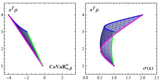
Figure 1: Images of functions ${x\mapsto\big{(}\mathop{\operatorname{CoVaR_{\alpha,\beta}^{=}}}(x),x^{\mathrm{T}}\mu\big{)}}$ (left) and ${x\mapsto\big{(}\operatorname{\sigma}(x),x^{\mathrm{T}}\mu\big{)}}$ (right) for ${x\in\{(x_{1},x_{2},x_{3})\in\mathbb{R}^{3}\mid x_{1}+x_{2}+x_{3}=1,\ x_{1}\geq 0,\ x_{2}\geq 0,\ x_{3}\geq 0\}}$.

Figure (1) might be of use both as an illustration and providing comparisons.

With one example without the counterpart of the critical line (2) the second one will be presented—this time with function $\mathop{\operatorname{CoVaR_{\alpha,\beta}^{=}}}$ attaining its minimum over $\{x\in\mathbb{R}^{n}\mid x_{1}+\dots+x_{n}=1\}$ which allows us to consider (6) both with and without the non-negativity constraint $(\star)$.

3.2 Example 2

$$(R_{1},R_{2},R_{3})\sim\mathcal{N}_{3}\left(\left(\begin{array}[]{ccccccc}2\\ 3\\ 1\\ \end{array}\right),\left(\begin{array}[]{rrr}1&1/5&1\\ 1/5&1&0\\ 1&0&9\\ \end{array}\right)\right),\quad a=1,\ b=2$$

In this case ${\mathop{\operatorname{CoVaR_{\alpha,\beta}^{=}}}(x)=1/5\Big{(}-5x_{1}-14x_{2}+2\sqrt{24x_{2}^{2}-10x_{2}x_{3}+200x_{3}^{2}\ }\Big{)}}$. Using just the ‘portfolio constraint’, $x_{1}+x_{2}+x_{3}=1$ from the optimization problem (6) generates a bounded below function with unique global minimum:

$$\left\{\begin{array}[]{lcccccc}\mathop{\operatorname{CoVaR_{\alpha,\beta}^{=}}}(x)\rightarrow\min\\ x_{1}+x_{2}+x_{3}=1\\ \end{array}\right.\quad\mbox{ gives us }x_{\min}=(1,0,0)^{\mathrm{T}},\ \mathop{\operatorname{CoVaR_{\alpha,\beta}^{=}}}(x_{\min})=-1.$$

3.3 Example 3

$$(R_{1},R_{2},R_{3})\sim\mathcal{N}_{3}\left(\left(\begin{array}[]{ccccccc}1\\ 2\\ 3\\ \end{array}\right),\left(\begin{array}[]{ccccccc}1&1&2\\ 1&9&0\\ 2&0&16\\ \end{array}\right)\right)$$

where:

$$\widehat{Q}=\left(\begin{array}[]{ccccccc}8&-2\\ -2&12\\ \end{array}\right)$$

This example is essentially an illustration of the dependence between values of $a,b$ and the obtained set of $\mathop{\operatorname{CoVaR_{\alpha,\beta}^{=}}}$-efficient portfolios. We have

$$\mathop{\operatorname{CoVaR_{\alpha,\beta}^{=}}}(x)=(a-1)x_{1}+(a-2)x_{2}+(2a-3)x_{3}+2b\sqrt{2x_{2}^{2}-x_{2}x_{3}+3x_{3}^{2}\,}.$$

Figure (2) presents five different possibilities, of which two first represent case $1$ in the theorem, two next—case $2$ and the last one case $3.$

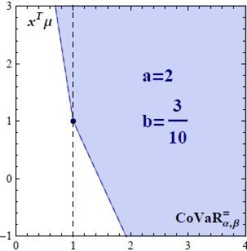
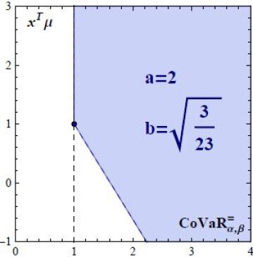
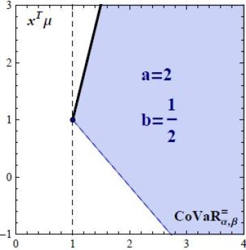
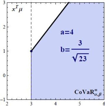
Figure 2: Images of ${x\mapsto\big{(}\mathop{\operatorname{CoVaR_{\alpha,\beta}^{=}}}(x),x^{\mathrm{T}}\mu\big{)}}$ for a choice of $(a,b)$.
The $\mathop{\operatorname{CoVaR_{\alpha,\beta}^{=}}}$-efficient frontiers are marked by thick lines.

4 Appendix: proofs $\&$ auxiliary results

4.1 Positive definiteness of $\hat{Q}$ and positive semidefiniteness of $Q$

For $\Sigma>0$ and ${e_{1}=\big{(}1,0,\dots,0\big{)}^{\mathrm{T}}}$ there is:

$$Q=\Sigma-\sigma_{1}^{-2}\,\Sigma e_{1}e_{1}^{\mathrm{T}}\Sigma=\Sigma\big{(}\Sigma^{-1}-\sigma_{1}^{-2}\,e_{1}e_{1}^{\mathrm{T}}\big{)}\Sigma.$$

Matrix ${e_{1}e_{1}^{\mathrm{T}}}$ has only one non-zero element (i.e. $1$ in first row, first column). In consequence ${\Sigma^{-1}-\sigma_{1}^{-2}\,e_{1}e_{1}^{\mathrm{T}}}$ has rank equal at least ${n-1}$ as its columns from second to last are the corresponding columns of $\Sigma^{-1}$. Therefore matrices $\hat{Q}$ and $Q$ are of the rank ${n-1}$, so that they are positive definite and positive semidefinite, respectively.
On the other hand, for $X=x^{\mathrm{T}}R$ and ${Y=R_{1}}$ we have

$$\forall x\in\{(x_{1},\widehat{x})\in\mathbb{R}^{n}\mid x_{1}\in\mathbb{R},\ \widehat{x}\in\mathbb{R}^{n-1}\}:\\ \widehat{x}^{\mathrm{T}\,}\widehat{Q}\widehat{x}=x^{\mathrm{T}\,}Qx=x^{\mathrm{T}\,}\Sigma x-x^{\mathrm{T}\,}q\,q^{\mathrm{T}\,}x=\sigma^{2}_{X}(1-\rho_{X,Y}^{2})\geq 0$$

so that ${\rho_{X,Y}^{2}=\pm 1}$ if and only if ${x=(const,0,\dots,0)^{\mathrm{T}}}$ (due to positive definiteness of $\widehat{Q}$) which in problem (4) implies ${x=(1,0,\dots,0)^{\mathrm{T}}}$.

4.2 Convexity of $\mathop{\operatorname{CoVaR_{\alpha,\beta}^{=}}}$ function

Function $s(\widehat{x})=\sqrt{\widehat{x}^{\mathrm{T}\,}\widehat{Q}\widehat{x}}$   is a norm induced by inner product ${\widehat{x}^{\mathrm{T}}\widehat{Q}\widehat{x}}$ and as such is convex on $\mathbb{R}^{n-1}$–indeed, due to $s$ being positively homogeneous of degree $1$, the Jensen’s inequality can be rewritten as:

$$\forall\widehat{x},\widehat{y}\in\mathbb{R}^{n-1},\forall\lambda\in[0,1]:\quad s\big{(}\lambda\widehat{x}+(1-\lambda)\widehat{y}\big{)}\leq s(\lambda\widehat{x})+s\big{(}(1-\lambda)\widehat{y}\big{)}$$ (8)

which is just triangle inequality, satisfied by every norm.

The fact that ${s(x_{2},0,\dots,0)=|x_{2}|\sqrt{\widehat{q}_{11}}}$ contradicts the strict convexity. However, as the inequality (8) is strict provided that ${\widehat{x}\nparallel\widehat{y}}$, function $s$ is strictly convex on every line segment not contained in any half-line with the origin as its element.

The instantaneous implication is that ${x^{\mathrm{T}}Qx=\widehat{x}^{\mathrm{T}}\widehat{Q}\widehat{x}}\,$ is convex on $\mathbb{R}^{n}$. Function ${\mathop{\operatorname{CoVaR_{\alpha,\beta}^{=}}}(x)=-x^{\mathrm{T}}\mu+a\,x^{\mathrm{T}}q+b\,\sqrt{x^{\mathrm{T}}Qx}}$ is convex as a linear combination of (proper) convex functions with positive coefficients.

4.3 A lemma about certain convex function

Lemma 1

Let us consider function ${F:\mathbb{R}\mapsto\mathbb{R}}$, ${F(t)=s\cdot t+\sqrt{(t-p)^{2}+q\,}}$ with ${s\in\mathbb{R}_{+}\cup\{0\},q\in\mathbb{R}_{+},\ p\in\mathbb{R}}$. Then ${F}$ is convex and the following is true:

1. For ${s\in[0,1)}$ there is a global minimum ${ps+\sqrt{q(1-s^{2})\,}}$ attained
   at ${t=p-s\sqrt{q(1-s^{2})^{-1}\,}}$

2. For ${s=1}$ there is no global minimum, but ${F(t)>\lim\limits_{\xi\rightarrow-\infty}F(\xi)=p}$

3. For $s>1$ function $F$ is not bounded below, ${\lim\limits_{\xi\rightarrow-\infty}F(\xi)=-\infty}$.

Proof via direct calculation.

4.4 Proof of the main theorem

For ${\mu,\mathbbm{1}_{n},q}$ linearly independent (which implies ${n\geq 3}$) we solve the following problem:

$$\left\{\begin{array}[]{lcccccc}\widehat{h}(\widehat{x})=1/2\,\widehat{x}^{\mathrm{T}}\widehat{Q}\widehat{x}\rightarrow\min\\ \widehat{x}^{\mathrm{T}}\widehat{\mu}=\widehat{E}\\ \widehat{x}^{\mathrm{T}}\widehat{q}=\widehat{t}\\ \end{array}\right.$$ (9)

and then vary the parameter $\widehat{t}$ in order to minimize the obtained solution with respect to $\widehat{t}$. Naturally, $\widehat{h}$ is strictly convex.

Via the method of Lagrange multipliers we get ${\widehat{Q}\widehat{x}=\lambda_{1}\widehat{\mu}+\lambda_{2}\widehat{q}}$. In consequence ${\widehat{x}=\lambda_{1}\widehat{Q}^{-1}\widehat{\mu}+\lambda_{2}\widehat{Q}^{-1}\widehat{q}}$. Left multiplication of first equation (by $\widehat{x}^{\mathrm{T}}$) and the second equation (by $\widehat{\mu}^{\mathrm{T}}$ and $\widehat{q}^{\mathrm{T}}$) gives us:

$$\widehat{x}^{\mathrm{T}}\widehat{Q}\widehat{x}= \lambda_{1}\widehat{E}+\lambda_{2}\widehat{t}$$ (10)

$$\widehat{E}= \lambda_{1}\,\alpha_{C}+\lambda_{2}\,\beta_{C}$$ (11)

$$\widehat{t}= \lambda_{1}\,\beta_{C}+\lambda_{2}\,\gamma_{C}$$ (12)

Scalars ${\lambda_{1},\lambda_{2}}$ are easily obtained from (11) and (12). Ultimately,

$${\widehat{x}^{\mathrm{T}}\widehat{Q}\widehat{x}=\Big{(}\widehat{E},\widehat{t}\,\Big{)}\cdot G^{-1}\cdot\Big{(}\widehat{E},\widehat{t}\,\Big{)}^{\mathrm{T}}},$$

where ${G}$ is the Gramian matrix of linearly independent vectors $\widehat{\mu},\widehat{q}$, with the inner product defined by matrix $\widehat{Q}^{-1}$ ($\widehat{Q}$ being positive definite implies positive definiteness of both $G$ and $G^{-1}$). Unless ${\widehat{E}=0}$ this quadratic function of $\widehat{t}$ is positive and bounded from $0$ (in the former case $0$ is attained for ${\widehat{t}=0}$ and equation (10) yields ${\widehat{x}=0}$). Then,

$$f(\widehat{x})=-\mu_{1}+a\,\sigma_{1}-\widehat{E}+a\,\widehat{t}+b\,\big{(}\alpha_{C}/\det G\big{)}^{1/2}\ \sqrt{\left(\widehat{t}-\beta_{C}/\alpha_{C}\,\widehat{E}\,\right)^{2}+\det G\cdot\widehat{E}^{2}/\alpha_{C}^{2}\,}$$

We take ${b^{-1}\big{(}\alpha_{C}/\det G\big{)}^{-1/2}\cdot\Big{(}f(\widehat{x})+\mu_{1}-a\,\sigma_{1}+\widehat{E}\Big{)}}$. Then the obtained function is of the type from lemma 4.3 with ${s=ab^{-1}\big{(}\det G/\alpha_{C}\big{)}^{1/2}}$. That means the global minimum is achieved for

$$\widehat{t}=\dfrac{\beta_{C}}{\alpha_{C}}\widehat{E}-|\widehat{E}|\,\dfrac{a\,\det G}{\alpha_{C}\sqrt{\Delta}},$$

under condition ${b>a\big{(}\det G/\alpha_{C}\big{)}^{1/2}}$ (i.e ${s<1}$) equivalent to ${\Delta>0}$ as ${a,b>0}$.

Then, ${\widehat{x}=\lambda_{1}\widehat{Q}^{-1}\widehat{\mu}+\lambda_{2}\widehat{Q}^{-1}\widehat{q}}$ yields formula for ${\widehat{x}(E)}$:

$$\widehat{x}(\widehat{E}) =\dfrac{\widehat{E}}{\alpha_{C}}\,\widehat{Q}^{-1}\widehat{\mu}+|\widehat{E}|\,\dfrac{a\,}{\alpha_{C}\sqrt{\Delta}}\,\widehat{Q}^{-1}(\beta_{C}\,\widehat{\mu}-\alpha_{C}\,\widehat{q}),$$

which is correct also for ${\widehat{E}=0}$ as ${\widehat{x}(0)=0}$. Formula for ${f\Big{(}\widehat{x}(\widehat{E})\Big{)}}$ comes as the obvious consequence:

$$f\Big{(}\widehat{x}(\widehat{E})\Big{)}=-\mu_{1}+a\,\sigma_{1}+\widehat{E}\left(\frac{a\,\beta_{C}}{\alpha_{C}}-1\right)+\frac{|\widehat{E}|}{\alpha_{C}}\sqrt{\Delta}.$$

Now we find $\mathop{\operatorname{CoVaR_{\alpha,\beta}^{=}}}$-efficient portfolios. The only ones that might satisfy the required conditions are ${x(\widehat{E})=(1-\mathbbm{1}_{n-1}^{\mathrm{T}}\widehat{x}(\widehat{E}),\widehat{x}(\widehat{E})^{\mathrm{T}})^{\mathrm{T}}}$ portfolios as graph of ${g(\widehat{E}):=f\Big{(}\widehat{x}(\widehat{E})\Big{)}}$ is the lower boundary of ${\{\big{(}x^{\mathrm{T}}\mu,\mathop{\operatorname{CoVaR_{\alpha,\beta}^{=}}}(x)\big{)}\mid x\in\mathbb{R}^{n}\}}$. Function $g(\widehat{E})$ is a continuous piecewise function comprising two linear functions. It can be easily observed that whether for a given $\widehat{E}$ portfolio ${x(\widehat{E})}$ is $\mathop{\operatorname{CoVaR_{\alpha,\beta}^{=}}}$-efficient depends solely on the ratio of ${a\,\beta_{C}/\alpha_{C}-1}$ and ${\alpha_{C}\sqrt{\Delta}}$, or, to be more specific, on the inequalities between ${a\beta_{C}-\alpha_{C}}$,${-\sqrt{\Delta}}$ and ${\sqrt{\Delta}}$.

4.5 Additional remarks

First note that without assuming linear independence of ${\mu,\mathbbm{1}_{n},q}$ there is ${q=\xi_{1}\mu+\xi_{2}\mathbbm{1}_{n}}$ (by previous assumption ${\mu}$ and ${\mathbbm{1}_{n}}$ are linearly independent). Therefore the optimization problem (7) would have the same critical set as that of Markowitz.

Observe also that for ${a\rightarrow 0}$ function $\widehat{x}(\widehat{E})$ converges to a linear function which is only to be expected by looking at the function defined in (7). Still, the problem is not equivalent to that of minimizing $\sigma$ (or $\mathop{\operatorname{VaR_{\alpha}}}$) as ${\sqrt{x^{\mathrm{T}}Qx}=\sqrt{\widehat{x}^{\mathrm{T}}\widehat{Q}\widehat{x}}}$, not ${\sqrt{x^{\mathrm{T}}\Sigma x}}$, is minimized. A linear function is achieved in no other way, as ${\widehat{\mu}\nparallel\widehat{q}}$ due to linear independence of ${\mu,\mathbbm{1}_{n},q}$. Therefore, the image of the ‘$\operatorname{CoVaR}^{=}$-critical polyline’  in ${E\mapsto\Big{(}E,f\Big{(}\widehat{x}(\widehat{E})\Big{)}\Big{)}}$ consist of two rays and with our assumption concerning $\Delta$ is never a line.

Now let ${\Delta=0}$ (i.e. ${s=1}$). Note here that ${p=\beta_{C}/\alpha_{C}\widehat{E}}$ from the lemma is not necessarily a positive number. Should we solve:

$$\left\{\begin{array}[]{lcccccc}\widehat{x}^{\mathrm{T}}\widehat{\mu}=\widehat{E}\\ \widehat{x}^{\mathrm{T}}\widehat{q}=\widehat{t}\\ \end{array}\right.$$

for any solution ${\widehat{x}_{\widehat{t}}(\widehat{E})}$ we would get ${g\big{(}\widehat{x}_{\widehat{t}}(\widehat{E})\big{)}\overset{\widehat{t}\rightarrow-\infty}{\longrightarrow}p}$ (solution being unique for given ${\widehat{t},\widehat{E}}$ only in case of ${n=3}$).

5 Future research

Present work but lightly touches the wide and complex subject of portfolio optimization for $\mathop{\operatorname{CoVaR_{\alpha,\beta}^{=}}}$. For any question answered few more are raised. What if the normality assumption was to be dropped? What if the Gauss distribution was to be replaced by another one? Will the results hold for $\operatorname{CoVaR}$? How solving the problem for various families of copulas, as done in Bernardi et al. [2017], would change the outcome? Also, Mainik and Schaanning [2014] show that $\mathop{\operatorname{CoVaR_{\alpha,\beta}^{=}}}$ is not monotonic with respect to $\rho_{X,Y}$—how badly does it affect the presented model?

References

- Adrian and Brunnermeier [2008] Adrian, T., Brunnermeier, M. K., 2008. Staff reports.
- Adrian and Brunnermeier [2016] Adrian, T., Brunnermeier, M. K., 2016. Covar. American Economic Review 106 (7), 1705–41.
- Alexander and Baptista [2002] Alexander, G. J., Baptista, A. M., 2002. Economic implications of using a mean-var model for portfolio selection: A comparison with mean-variance analysis. Journal of Economic Dynamics and Control 26 (7), 1159–1193.
- Alexander and Francis [1986] Alexander, G. J., Francis, J. C., 1986. Portfolio Analysis. Prentice-Hall foundations of finance series. Prentice-Hall.
- Artzner et al. [1999] Artzner, P., Delbaen, F., Eber, J.-M., Heath, D., 1999. Coherent measures of risk. Mathematical finance 9 (3), 203–228.
- Bernardi et al. [2017] Bernardi, M., Durante, F., Jaworski, P., 2017. Covar of families of copulas. Statistics & Probability Letters 120, 8–17.
- Black [1972] Black, F., 1972. Capital market equilibrium with restricted borrowing. The Journal of Business 45 (3), 444–455.
- Mainik and Schaanning [2014] Mainik, G., Schaanning, E., 2014. On dependence consistency of covar and some other systemic risk measures. Statistics & Risk Modeling 31 (1), 49–77.
- Markowitz [1952] Markowitz, H., 1952. Portfolio selection. The Journal of Finance 7 (1), 77–91.
- Markowitz [1959] Markowitz, H., 1959. Portfolio Selection: Efficient Diversification of Investments. New York : Wiley.
- Merton [1972] Merton, R. C., 1972. An analytic derivation of the efficient portfolio frontier. Journal of financial and quantitative analysis 7 (04), 1851–1872.
- Rockafellar and Uryasev [2000] Rockafellar, R. T., Uryasev, S., 2000. Optimization of conditional value-at-risk. Journal of risk 2, 21–42.