Accurate parameters for HD 209458 and its planet from HST spectrophotometry

Abstract

We present updated parameters for the star HD 209458 and its transiting giant planet. The stellar angular diameter $\theta$=0.2254$\pm$0.0017 mas is obtained from the average ratio between the absolute flux observed with the Hubble Space Telescope and that of the best-fitting Kurucz model atmosphere. This angular diameter represents an improvement in precision of more than four times compared to available interferometric determinations. The stellar radius $R_{\star}$=1.20$\pm$0.05 R_☉ is ascertained by combining the angular diameter with the Hipparcos trigonometric parallax, which is the main contributor to its uncertainty, and therefore the radius accuracy should be significantly improved with Gaia’s measurements. The radius of the exoplanet $R_{\text{p}}$=1.41$\pm$0.06 $R_{\text{J}}$ is derived from the corresponding transit depth in the light curve and our stellar radius. From the model fitting, we accurately determine the effective temperature, $T_{\text{eff}}$=6071$\pm$20 K, which is in perfect agreement with the value of 6070$\pm$24 K calculated from the angular diameter and the integrated spectral energy distribution. We also find precise values from recent Padova Isochrones, such as $R_{\star}$=1.20$\pm$0.06 R_☉ and $T_{\text{eff}}$=6099$\pm$41 K. We arrive at a consistent picture from these methods and compare the results with those from the literature.

1 Introduction

Accurate stellar radii are required to determine accurate planetary radii from (spectro-)photometric transits. Long-baseline optical/infrared interferometry provides the most direct way to ascertain stellar angular diameters, but it is limited to relatively nearby and bright stars (e.g.: van Belle & von Braun, 2009; Baines et al., 2009; van Braun et al., 2014; Boyajian et al., 2015; Ligi et al., 2015).

Recently, Allende Prieto & del Burgo (2016) have shown that the comparison of absolute flux spectrophotometry of A stars from the STIS Next Generation Spectral Library (NGSL; Gregg et al., 2006) with appropriate stellar atmosphere models leads to angular diameters that are more accurate than those from interferometry. Both methods require accurate parallaxes to finally achieve precise stellar radii.

Measurements of parallaxes from ground-based instruments are subject to distortions due to the Earth’s atmosphere. Observations from space overcome this problem. ESA’s Hipparcos was the first space mission fully dedicated to determine precise positions, distances, proper motions, and luminosities for more than 118,000 stars brighter than V=12.4 mag (ESA, 1997; van Leeuwen, 2007) over the entire sky. Hipparcos has had a remarkable impact in many different areas of Astronomy. ESA’s Gaia, launched in 2013, is collecting astrometric, photometric, and spectroscopic data for about 10⁹ stars with 3$\la$V$\la$20 mag with a much higher precision in position accuracy and much higher sensitivity than Hipparcos.

HD 209458 is a nearby (parallax $\Pi$=20.15$\pm$0.80 mas, van Leeuwen, 2007) G0V star with an estimated age of 4$\pm$2 Gyr (Melo et al., 2006). It has been recently observed with the CHARA Array interferometer, finding that its limb-darkened angular diameter is $\theta_{\text{LD}}$= 0.225$\pm$0.007 mas (Boyajian et al., 2015). It harbors HD 209458 b, the first transiting planet discovered (Charbonneau et al., 2000). This is a short period inflated planet that has challenged planet formation theories (Mardling, 2007). HD 209458 is also one of only two systems with absolute stellar and planetary masses derived from high resolution spectroscopy (Snellen et al., 2010). The other is HD 189733 (de Kok et al., 2013).

Modeling the Spectral Energy Distribution (SED) of G-type stars is relatively easy in the optical and infrared, where the continuum opacity is dominated by H^- bound-free and free-free absorption, but becomes increasingly harder in the ultraviolet due to the accumulation of spectral lines, the complex contribution of bound-free opacity from neutral atoms, and the shift of the line formation from the photosphere to higher atmospheric layers.

HD 209458 was observed with the instruments STIS and NICMOS onboard NASA/ESA Hubble Space Telescope (HST). Observing from space avoids the scintillation noise resulting from air turbulence in the Earth’s atmosphere, yielding an improvement of up to three orders of magnitude in (spectro-)photometric precision. Moreover, the limitations owing to the day-night cycle and variable weather conditions are eliminated.

In this paper we present results based on the analysis of the HST spectrophotometry of HD 209458. Section 2 describes the observed and modeled spectra, and the evolutionary models used here. In Section 3, the analysis and results on the properties of this host star and its planet are explained, including an accurate effective temperature for HD 209458 and the most accurate to date nearly model-independent radii for the star and its planet. This section also includes a comparison of our results with those in the literature. Section 4 is devoted to a discussion on the potential precision and accuracy expected for the applied technique and a comparison with others. Finally, Section 5 presents our conclusions.

2 Observed and modeled spectra

2.1 Absolute spectrophotometry

The HST archive contains STIS CCD first order spectroscopy (G430L, G750M, and G750L) and NICMOS slitless grism imaging spectroscopy (G096, G141, and G206) for HD 209458. The reduced data were downloaded from the CALSPEC Calibration Database, which contains the composite stellar spectra for the flux standards on the HST system.

STIS data are fairly homogeneous, even though their wide spectral coverage relies on using different gratings. The expected resolving power $R$ varies slightly with wavelength, as described in the STIS Instrument Handbook. According with the NICMOS Instrument Handbook the resolving power is $R\sim$ 200 per pixel over the full field of view of the camera. We found the FWHM values in the FITS header of the CALSPEC spectrum for HD 209458 to be smaller than those needed to match this spectrum in the ultraviolet and visible (R$\approx$560-700). Therefore, we applied our own estimates of FWHM for each grating to properly smooth our theoretical models before comparing them to the observations.

2.2 Stellar atmosphere models

We computed synthetic spectra covering the wavelength range 0.2–2.5 $\mu$m with wavelength steps equivalent to 0.3 km s^-1. The calculations are based on Kurucz ATLAS9 model atmospheres (Mészáros et al., 2012) and the synthesis code ASS$\epsilon$T (Koesterke et al., 2008; Koesterke, 2009), operated in 1D (plane-parallel geometry) mode. The reference solar abundances adopted in the model atmosphere and the synthesis are from Asplund et al. (2005).

The equation of state includes the first 92 elements in the periodic table and 338 molecules (Tsuji, 1964, 1973, 1976, with some updates). Partition functions are adopted from Irwin (1981). Bound-free absorption from H, H^-, HeI, HeII, and the first two ionization stages of C, N, O, Na, Mg, Al, Si, Ca (from the Opacity Project; see Cunto et al., 1993) and Fe (from the Iron Project; Bautista, 1997; Nahar, 1995) are included. Line absorption is modeled in detail using the atomic and molecular (H₂, CH, C₂, CN, CO, NH, OH, MgH, SiH, and SiO) files compiled by Kurucz.

Level dissolution near the Balmer series limit is accounted for (Hubeny et al., 1994). The radiative transfer calculations include Rayleigh (H; Lee & Kim, 2004) and electron (Thomson) scattering. The damping of H lines are treated in detail using Stark (Stehlé, 1994; Stehlé & Hutcheon, 1999) and self-broadening (for Balmer Barklem et al., 2000; Ali et al., 1966, for Lyman and Paschem lines).

To ease the derivation of atmospheric parameters from the HST spectrophotometry, we computed a grid of model surface fluxes for effective temperatures in the range 5750 $\leq T_{\text{eff}}\leq$ 10,000 K, surface gravity 1.0 $\leq\log g\leq$ 5.0 ($g$ in cm s^-2), microturbulence -0.3 $\leq\log\xi_{t}\leq$ 0.9 ($\xi_{t}$ in km s^-1), metallicity -5 $\leq$ [Fe/H] $\leq$ +1.0, and $\alpha$-element enhancement -1.0 $\leq$ [$\alpha$/Fe] $\leq$ +1.0, in steps of 250 K, 0.5 dex, 0.3 dex, 0.25 dex, and 0.25 dex, respectively. Spectra were convolved with a series of Gaussian kernels (see §2.1) to account for instrumental broadening. The effect of interstellar reddening was considered following Fitzpatrick (1999).

2.3 Stellar evolution models

We employed the PARSEC (stellar tracks and isochrones with the PAdova & TRieste Stellar Evolution Code) Isochrones (version 1.2S: Bressan et al., 2012; Chen et al., 2014, 2015; Tang et al., 2014), with two different grids adequate to derive the stellar properties of the Sun and our target of interest. In the first grid, which is used to calibrate the system (given that HD 209458 is particularly similar to the Sun), the initial metallicity $Z_{\text{ini}}$ ranges from 0.0151 to 0.0211, in steps of 0.0005, age ($\tau$) from 4.1 to 5.3 Gyr, in steps of 0.01 Gyr, and initial mass ($M_{\text{ini}}$) ranging from 0.09 M_☉ to the highest mass established by the stellar lifetime, in steps of 10^-4 M_☉. In the second grid, $Z_{\text{ini}}$ goes from 0.0046 to 0.0246, in steps of 0.005, $\tau$ from 0.1 to 12.1 Gyr, in steps of 0.3 Gyr, and $M_{\text{ini}}$ spans from 0.09 M_☉ to the highest mass given the stellar lifetime, in steps of 2 10^-3 M_☉.

The PARSEC models include the evolution of a star from its formation to the asymptotic giant branch phase for low- and intermediate mass stars, or the carbon ignition phase for massive stars. The age ruler by these models includes the pre-main sequence lifetime, which is about 40 Myr for the Sun and slightly lower for HD 209458. These models provide, among other stellar parameters, actual mass, luminosity, effective temperature, surface gravity, bolometric magnitude, and magnitudes in a chosen photometric system (Johnson-Cousins for this research) as a function of the stellar age, metallicity, and the initial mass. The radius can be trivially calculated from the mass and gravity, and the mean density from the mass and radius. We only used the photometric bands $B$ and $V$ provided by PARSEC, which were obtained with the responses and zero points derived by Maíz Apellániz (2006). The corresponding stellar parameters for the regular sampling in M${}_{\text{ini}}$ were computed from the tabulated values using linear interpolation.

3 Analysis and results

3.1 Spectral analysis

We searched for the values of $T_{\text{eff}}$, $\log g$, [Fe/H], [$\alpha$/Fe], and $\xi_{t}$, associated with the model fluxes that best fit the spectrum of HD 209458 in the wavelength range from 0.29 to 2.5 $\mu$m. For this fit we divided both observations and models, resampled on the same wavelength grid, by their own mean fluxes. Interstellar extinction was considered as well, finding that the optimal solution led to a negative value ($E(B-V)$ = -0.09 mag), and therefore was neglected given the proximity of HD 209458 ($\sim$50 pc). This is in agreement with the small value $E(B-V)$=0.003 mag found from the same HST data by Bohlin et al. (2014), who noted that the CALSPEC data for this star agrees with its preferred model to $\sim$2%.

We defined three wavelength regions of interest: ultraviolet (UV: 0.29-0.50 $\mu$m), visible (VIS: 0.50-1.0 $\mu$m), and near-infrared (NIR: 1.0-2.5 $\mu$m). We performed fittings to VIS-NIR, VIS, UV-VIS-NIR, and UV-VIS, allowing all stellar parameters to vary (all/free), fixing $\log g$ (g/fixed), and fixing all parameters except $T_{\text{eff}}$ ($T_{\text{eff}}$/free). In this way, we could gauge the achieved accuracy and precision for determining stellar parameters for the different cases.

Table 1: Stellar parameters and 1$\sigma$ uncertainties of HD 209458 obtained from different methods: 1) BF: Best-fitting Kurucz model atmosphere to ascertain $T_{\text{eff}}$, $\theta$ (through the comparison with the observed spectrum), and $R_{\star}$ (using $\theta$ and $\Pi$). $L_{\star}$ is then calculated from $R_{\star}$ and $T_{\text{eff}}$; 2) Procedure based on the bolometric flux to determine $T_{\text{eff}}$ using the theoretical model ($f_{\text{bol}}$-mod) and the observed spectrum ($f_{\text{bol}}$-obs) in combination with $\theta$. Also to obtain $L_{\star}$ using $\Pi$; 3) EM: Search for PARSEC (version 1.2S) evolution models using the likelihood function ${\mathcal{L}}$; 4) Determination of $\log g$ from $R_{\star}$ (using BF) and either $\rho_{\star}$ derived from the light curve (BF-LC) or $M_{\star}$ derived from the PARSEC models (BF-EM). BF-LC and BF-EM also permit to calculate $M_{\star}$ and $\rho_{\star}$, respectively. SynPhot: Synthetic photometry in the Johnson-Cousins $UBVRI$ and 2MASS systems extracted from the CALSPEC spectrum of this star.

Parameter	Value$\pm$uncertainty	Note
$T_{\text{eff}}$ (K)	6071$\pm$20	BF; see §3.1
$\shortparallel$	6070$\pm$24	$f_{\text{bol}}$-mod; see §3.5
$\shortparallel$	6064$\pm$24	$f_{\text{bol}}$-obs; see §3.5
$\shortparallel$	6099$\pm$41	EM; see §3.8
$\theta$ (mas)	0.2254$\pm$0.0017	BF; see §3.3
$R_{\star}$ (R☉)	1.20$\pm$0.05	BF; see §3.4
$\shortparallel$	1.20$\pm$0.06	EM; see §3.8
$L_{\star}$ (L☉)	1.77$\pm$0.14	$f_{\text{bol}}$-mod; see §3.6
$\shortparallel$	1.76$\pm$0.14	$f_{\text{bol}}$-obs; see §3.6
$\shortparallel$	1.77$\pm$0.14	BF; see §3.6
$\shortparallel$	1.79$\pm$0.14	EM; see §3.8
$M_{\text{bol}}$ (mag)	4.11$\pm$0.09	EM; see §3.8
$\log g$ [cm s-2]	4.38$\pm$0.06	BF-LC; see §3.7
$\shortparallel$	4.33$\pm$0.04	BF-EM; see §3.7
$\shortparallel$	4.33$\pm$0.04	EM; see §3.8
$M_{\star}$ (M☉)	1.26$\pm$0.15	BF-LC; see §3.7
$\shortparallel$	1.12$\pm$0.04	EM; see §3.8
$\rho_{\star}$ (g cm-3)	0.91$\pm$0.11	BF-EM; see §3.7
$\shortparallel$	0.91$\pm$0.14	EM; see §3.8
$\tau$ (Gyr)	3.5$\pm$1.4	EM; see §3.8
$U$	8.235	SynPhot; see §3.2
$B$	8.204	$\shortparallel$
$V$	7.655	$\shortparallel$
$R$	7.342	$\shortparallel$
$I$	7.037	$\shortparallel$
$J$	6.635	$\shortparallel$
$H$	6.346	$\shortparallel$
$K_{s}$	6.326	$\shortparallel$

The optimization was done using the FORTRAN90 code FER R E (Allende Prieto et al., 2006) using the Unconstrained Optimization BY Quadratic Approximation (UOBYQA) algorithm (Powell, 2002). Model fluxes with any set of atmospheric parameters are derived by cubic Bezier interpolation (see Auer, 2003, and references therein) in the grid of model fluxes described in §2.2.

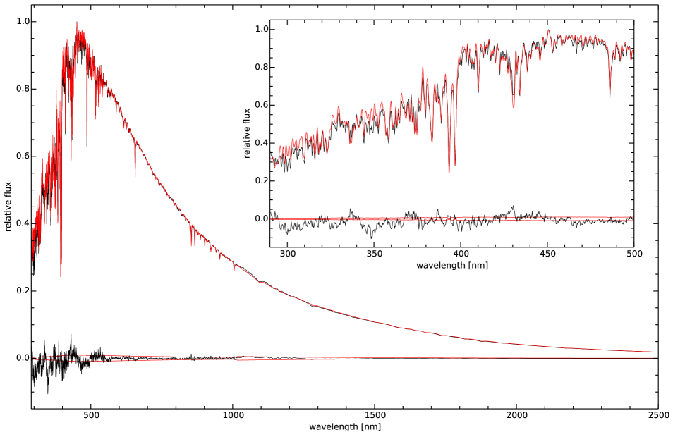
Figure 1: HST spectrum (solid black line) and best-fitting model (solid red line) for HD 209458. Also, at the bottom the residuals (black line) and the 1$\sigma$ uncertainties for the flux (red lines), stored in the FITS header of the CALSPEC spectrum. The spectra, residuals, and uncertainties between 290 and 500 nm are also zoomed.

STIS spectra have been proven to be very useful to ascertain angular diameters of A-type stars, but a free parameter fitting does not necessarily provide accurate values of e.g., surface gravity (Allende Prieto & del Burgo, 2016). For HD 209458, the fitting with the lowest value for chi-square ($\chi^{2}$) was that of VIS-NIR-all/free, but the extracted parameters ($T_{\text{eff}}$=6125 K, $\log g$=4.78, [Fe/H]=-0.19) have extreme values (the highest ones for $T_{\text{eff}}$ and $\log g$, and the second lowest one of [Fe/H] among all fittings). Since our goal is to derive appropriate parameters of the star, a fitting was performed fixing all parameters but $T_{\text{eff}}$, which must be well constrained given the broad wavelength range.

We indeed argue that VIS-$T_{\text{eff}}$/free is our best fitting ($T_{\text{eff}}$=6071 K, $\log g$=4.38, [Fe/H]=0, [$\alpha$/Fe]=0, $\log\xi_{t}$=0.04) because: 1) The VIS spectrum has a high signal-to-noise and many absorption lines that are very well modeled, in contrast to the complex UV and the fainter nearly-featureless NIR; and 2) The zero-point of the flux scale is very well constrained in the visible (see §3.2). We estimated an uncertainty in $T_{\text{eff}}$ of 20 K, which is based on: 1) The differences between VIS-g/fixed and VIS-NIR-g/fixed (increase of $\approx$20 K) and UV-VIS-NIR-g/fixed (same value); and 2) The increment between VIS-$T_{\text{eff}}$/free and VIS-NIR-$T_{\text{eff}}$/free amounts to $\approx$15 K, and the decrease with respect to UV-VIS-NIR-$T_{\text{eff}}$/free is of $\approx$50 K. The UV cannot be fitted as well as the optical, mainly due to the crowding of lines and continuum absorption by metals.

Therefore, our best fitting model (reduced chi-square $\chi^{2}_{\text{red}}$=0.462; N=1096 data points) to the CALSPEC spectrum relies on the VIS region, arriving at $T_{\text{eff}}$=6071$\pm$20 K (see Table 1). Fig. 1 shows the modeled and observed spectra. We note the flux uncertainties (systematic and statistical) from the FITS header of the CALSPEC spectrum are overestimated by $\sim$50% in the VIS region, which is inferred from the comparison of these flux uncertainties with the residuals between the observed and modeled spectra. This explains the low estimate of $\chi^{2}_{\text{red}}$. In most of the UV the residuals are significantly larger than the estimated uncertainties stored in the FITS header of the HD 209458 spectrum, confirming the difficulties to model this region. Conversely, the residuals in the NIR fall within the estimated flux uncertainties.

3.2 Photometry

We computed the Johnson-Cousins and 2MASS photometry from the CALSPEC spectrum of HD 209458 (see Table 1). We adopted the Optimized Bessel Bandpass Functions presented by Bohlin & Landolt (2015). These correspond to the $UBVRI$ response curves of Bessell & Murphy (2012) shifted by up to -31 Å to minimize the differences between the Landolt photometry and the synthetic CALSPEC photometry of 11 spectrophotometric flux standards. The uncertainty of the monochromatic flux at 555.75 nm (555.6 nm in air) is 0.5% or 0.005 mag (see Bohlin et al., 2014, and the CALSPEC Calibration Database). Table 5 of Bohlin & Landolt (2015) lists the magnitudes and uncertainties for the conversion to magnitudes of Vega on the Johnson-Cousing system. For example, $V$=0.028 mag, rms=0.005, and uncertainty in the mean of 0.003 mag. These magnitudes for Vega were confirmed with our code, with differences below 0.001 mag.

The values so obtained for HD 209458, $B$=8.204$\pm$0.010 and $V$=7.655$\pm$0.008 mag, are slightly different from those computed using the response curves of Maíz Apellániz (2006), which lead to $B$ = 8.212 and $V$ = 7.649, but such differences are within the 1$\sigma$ uncertainties. Our value of $V$ is similar to that of $V$=7.65 mag from Bohlin (2010) and slightly larger than that from Bohlin et al. (2014) of $V$=7.63. It is also in agreement with the value of $V$=7.65$\pm$0.01 given by Torres et al. (2008).

The 2MASS $J$, $H$, and $K_{s}$ photometry was extracted from the CALSPEC spectrum using the response curves and zero points from Cohen et al. (2003a). Our values of $J$=6.635, $H$=6.346, and $K_{s}$=6.326 are in fair agreement with those of $J$=6.591$\pm$0.020, $H$=6.37$\pm$0.04, and $K_{s}$=6.308$\pm$0.026 from Cutri et al. (2003). Given the uncertainties in the 2MASS passbands, absolute values of differences correspond to $\sim$2$\sigma$, $\sim$0.5$\sigma$, and $\sim$0.5$\sigma$, respectively.

There are different response curves for the Johnson and Cousins systems in the literature, yielding different synthetic magnitudes extracted from a certain model spectrum. Apart from the above-mentioned Optimized Bessel Bandpass Functions, we have employed the response curves from Cohen et al. (2003b), Maíz Apellániz (2006), and Mann & von Braun (2015) to compute the magnitudes of HD 209458 in the $UBVRI$ filter-bands. The differences between the maximum and minimum extracted values are 0.09, 0.016, 0.02, 0.03, and 0.013 mag for $U$, $B$, $V$, $R$, and $I$, respectively. The most extreme differences are 0.09 mag in the $U$ band. Note that bandpass functions may be multiplied by a mean atmospheric transmission spectrum appropriate for a certain observing site (e.g., Cohen et al., 2003b, for CTIO, Chile). Earth’s atmospheric transmission variations lead to systematic errors in the UV. This has an impact on the results from model atmosphere fittings to broad-band photometry, together with the reduced number of points used to constrain the solution. Our technique overcomes this problem, since it uses the high signal-to-noise CALSPEC spectrum, which is absolutely calibrated in flux and presents $\simeq$550 resolved elements in the wavelength range between 500 and 1000 nm ($\simeq$1030 resolved elements in the full wavelength range of STIS and NICMOS).

3.3 Stellar angular diameter

In a similar way to del Burgo et al. (2010) and Allende Prieto & del Burgo (2016) the angular diameter $\theta\simeq 2R/d=2\sqrt{f/F}$ for HD 209458 was determined from the average ratio $<f/F>$ between the flux observed and that predicted by the model at the stellar surface in the 0.5-1.0 $\mu$m wavelength range. We used the best fitting model obtained in §3.1 ($T_{\text{eff}}$=6071  K, $\log g$= 4.38, [Fe/H]=0, [$\alpha$/Fe]=0, $\log\xi_{t}$=0.04) and find the angular diameter to be $\theta$=0.2254$\pm$0.0017 mas (see Table 1). Our value is more precise than the interferometric one of 0.225$\pm$0.007 mas from Boyajian et al. (2015). It is also better than the value of 0.224$\pm$0.004 mas determined by Casagrande et al. (2010) with a methodology similar to ours, probably due to the use of approximate SEDs provided with the model atmospheres adopted in their analysis. Fig. 2 shows $\theta$ versus wavelength, where it is observed that the fitting based on the VIS region is very good in the full spectral range. Indeed, we found a very similar value for the stellar angular diameter in the wavelength ranges VIS and VIS-NIR.

The uncertainty $\sigma(\theta)$ is quantified by adding in quadrature three terms: 1) a random error contribution estimated from the scatter of the flux ratio across the selected wavelength interval (0.0008 mas); 2) the error in the spectral shape because of the uncertainties in the stellar parameters, which is computed from a MonteCarlo approach with 100 trials (0.0014 mas); and 3) the error contribution of 0.25% that corresponds to propagating the uncertainty of the flux scale of 0.5% in the zero-point (0.0006 mas).

Our result is largely model-independent, since the impact of the uncertainties in the parameters describing the model is moderately low. The uncertainties introduced to derive this component of $\sigma(\theta)$ are $\sigma(T_{\text{eff}})$=20 K, $\sigma(\log g)$=0.06 dex, and $\sigma$([Fe/H])=0.05 dex. We found $\sigma(T_{\text{eff}})$ to be the major contributor, while the effect of $\sigma(\log g)$ is negligible.

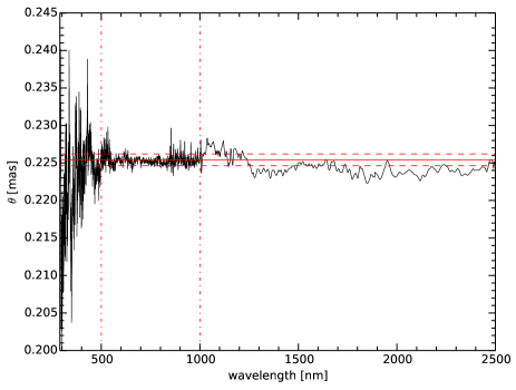
Figure 2: Angular diameter $\theta\simeq 2\sqrt{f/F}$ versus wavelength. The vertical dash-dotted lines indicate the wavelength limits used to obtain the mean value of $\theta$ and its standard deviation, which are marked by the continuous line and dashed lines, respectively. Note that although the fitting is applied to the VIS region, the match is very good in the full wavelength range. The total uncertainty in $\theta$ was calculated quadratically adding to the above-mentioned standard deviation the contributions from the error in the zero-point on the flux scale and the error in the spectral shape due to the uncertainties in the stellar parameters (see §3.3).

For A-type stars, we found that the values of $\log g$ and [Fe/H] derived from spectral fitting depend heavily on the Balmer and Paschen jumps, and the near-UV line absorption, respectively (Allende Prieto & del Burgo, 2016). In that study some of the extracted values for $\log g$ were lower (by up to 0.5 dex) than those ascertained from stellar structure models. However, metallicity and surface gravity (as well as the effective temperature) have a very limited impact on the spectral energy distribution of A-type stars in the wavelength range 0.40-0.80 $\mu$m (see also del Burgo et al., 2010). Our analysis for the G-type star HD 209458 relies on an accurate determination of $T_{\text{eff}}$ and $\log g$, which is fixed in our fitting. This leads to a slightly higher value of $\sigma(\theta)$ compared to that derived from an analysis in which all parameters are free to vary.

3.4 Stellar radius

Combining the angular diameter obtained in the previous section with the trigonometric parallax from Hipparcos ($\Pi$=20.15$\pm$0.80 mas, van Leeuwen, 2007) for HD 209458 we derive the stellar radius $R_{\star}$=1.20 $\pm$ 0.05 R_☉ (see Table 1). This value is in excellent agreement with that from Boyajian et al. (2015) (1.20$\pm$0.06 R_☉), obtained from their limb-darkened angular diameter and the Hipparcos parallax. But we also found our result to be consistent with others from stellar evolution models such as those from Bonfanti et al. (2015) (1.20$\pm$0.04 R_☉), Torres et al. (2008) (1.155${}^{+0.014}_{-0.016}$ R_☉), and our own analysis described in §3.8 (1.20$\pm$0.06 R_☉). Note our precision is similar to that of Bonfanti et al. (2015), who employed PARSEC (version 1.0, Bressan et al., 2012), but quite different to that of Torres et al. (2008), who used Yonsei-Yale (Y²) series by Yi et al. (2001) constrained by [Fe/H], $T_{\text{eff}}$, and $\frac{a}{R_{\star}}$ ($a$ is the semi-major axis of the orbit) using a likelihood function.

3.5 Bolometric flux and effective temperature

We determined the bolometric flux $f_{\text{bol}}$ = (2.289$\pm$0.011) $\times$ 10^-8 erg cm^-2 s^-1 from the integration between 0.29 and 300 $\mu$m of the HD 209458 spectrum, extended towards the UV ($\lambda<$ 0.29 $\mu$m) with a Kurucz model with $T_{\text{eff}}$=6071  K. The fluxes beyond 2.5 $\mu$m come from a Kurucz model introduced to complete the SED (Bohlin, 2010). The ultraviolet and infrared portions added to the SED respectively contribute only 1.6% and 2.9% of the total flux. The use of different models (with other stellar parameters values within the uncertainties) to complete the observed STIS+NICMOS spectrum has a negligible effect on the results presented here.

Alternatively, we obtained $f_{\text{bol}}$= (2.298$\pm$0.011) $\times$ 10^-8 erg cm^-2 s^-1 from the best model derived in §3.1. Any of our values of $f_{\text{bol}}$ (which are consistent with each other) is $\sim$5 times more precise than that of Boyajian et al. (2015) with $f_{\text{bol}}$= (2.33$\pm$0.05) $\times$ 10^-8 erg cm^-2 s^-1, which they derived from a model fitted to broad-band photometry collected from the literature. Casagrande et al. (2010) arrived at $f_{\text{bol}}$= (2.335$\pm$0.025) $\times$ 10^-8 erg cm^-2 s^-1, adopting [Fe/H] = 0.03$\pm$0.02, $\log g$=4.50$\pm$0.04, Tycho 2, and 2MASS photometry.

From the bolometric flux we determine the effective temperature ($T_{\text{eff}}=\left(\frac{4f_{\text{bol}}}{\sigma\theta^{2}}\right)^{0.25}$, where $\sigma$ is the Stefan-Boltzmann constant). We have thus found the effective temperature to be $T_{\text{eff}}$=6064$\pm$24 K from the CALSPEC spectrum, and 6070$\pm$24 K from the best-fitting model, in consonance with that derived in §3.1. These results (compiled in Table 1) demonstrate the high precision of the spectral shape and flux zero-point of the HST data, as well as the excellent match to our best-fitting stellar atmosphere model. Boyajian et al. (2015) found that $T_{\text{eff}}$=6092$\pm$103 K from their $f_{\text{bol}}$ and interferometric limb-darkened angular diameter, and Casagrande et al. (2010) obtained $T_{\text{eff}}$=6113$\pm$49 K. Our more precise $f_{\text{bol}}$ and $\theta$ (see §3.3) lead to a significantly more precise value for the effective temperature.

3.6 Stellar luminosity

First, we determined the stellar luminosity from the bolometric flux and the Hipparcos parallax (L $\propto\frac{f_{\text{bol}}}{\Pi^{2}}$), which leads to $L_{\star}$=1.76$\pm$0.14 L_☉ and 1.77$\pm$0.14 L_☉ using the values of $f_{\text{bol}}$ obtained from the observed and theoretical spectrum, respectively (see §3.5). Note $\sigma(L_{\star})$ is dominated by the uncertainty in the parallax. Alternatively, it is found that $L/L_{{\sun}}=\left(R/R_{\sun}\right)^{2}\left(T_{\text{eff}}/T_{\text{eff},{\sun}}\right)^{4}$, yielding $L_{\star}$=1.77$\pm$0.14 L_☉ from $R_{\star}$ (see §3.4) and $T_{\text{eff}}$ (see §3.1). These values are compiled in Table 1.

Our results are in good agreement with the values of $L_{\star}$=1.79$\pm$0.15 L_☉ and $L_{\star}$=1.77$\pm$0.01 L_☉ from Boyajian et al. (2015) and Bonfanti et al. (2015), respectively. The former is obtained from a model atmosphere fitting to broad-band photometry and the latter is based on stellar evolutionary models. Our value of $L_{\star}$=1.79$\pm$0.14 L_☉ derived from PARSEC models (see §3.8) is also consistent with all these values. Note, however, the very small uncertainty in the luminosity given by Bonfanti et al. (2015) even though they used Padova Isochrones (version 1.0). Also from stellar evolutionary models, Torres et al. (2008) found a relatively low value of $L_{\star}$=1.62$\pm$0.10 L_☉, but it is still in agreement with the others.

3.7 Stellar mass, mean density and gravity

We applied two different approaches to determine two of three stellar parameters (mean density, mass, and gravity) from the stellar radius (see §3.4) combined with either the mass or the mean density from the literature or from the PARSEC models (see §3.8). First, given the radius and the mass, we found the mean stellar density to be $\rho=\frac{3M}{4\pi R^{3}}$ and gravity $g=\frac{GM}{R^{2}}$, where $G$ is the gravitational constant. There is good agreement among results for the stellar mass $M_{\star}$=1.11$\pm$0.02 M_☉ (Bonfanti et al., 2015), 1.12$\pm$0.03 M_☉ (Torres et al., 2008), and 1.12$\pm$0.04 M_☉ (see §3.8). We used our values of $M_{\star}$ (see §3.8) and $R_{\star}$ (see §3.4) to arrive at $\rho_{\star}$=0.91$\pm$0.11 g cm^-3 and $\log g$= 4.33$\pm$0.04 (with $g$ in cm s^-2) (see Table 1).

Second, we used our stellar radius and a value for the mean stellar density ascertained by Torres et al. (2008) from the (high signal-to-noise) HST/STIS transit light curve (Brown et al., 2001). Torres et al. (2008) determined $\rho_{\star}$=1.024$\pm$0.014 g cm^-3 from the expression $\rho_{\star}=\frac{3\pi}{GP^{2}}\left(\frac{a}{R_{\star}}\right)^{3}-\rho_{\text{p}}\left(\frac{R_{\text{p}}}{R_{\star}}\right)^{3}$, inserting the semi-major to stellar radius ratio $\frac{a}{R_{\star}}$ and the period $P$. They neglected the second term, which is generally very small because the planetary radius $R_{\text{p}}\ll{R_{\star}}$. From this mean stellar density and our $R_{\star}$ we calculated $M_{\star}$=1.26$\pm$0.15 M_☉ and more significantly $\log g$=4.38$\pm$0.06 ($g$ in cm s^-2) (see Table 1). The estimated value for the uncertainty of $\log g$ derived in §3.8 is smaller, but we argue that $\log g$=4.38$\pm$0.06 (with $g$ in cm s^-2) is more accurate and nearly model-independent, so we decided to use it as a fixed parameter in the fitting process described in §3.1.

3.8 Isochrones

Table 2: Stellar parameters ($T_{\text{eff}}$, $\log g$, $\tau$, $L$, $M_{\text{bol}}$, $M$, $R$, and $\rho$) and 1$\sigma$ uncertainties for the Sun inferred from our method on the PARSEC models for the initial solar metallicity from Bressan et al. (2012), $M_{\text{V}}$=4.862$\pm$0.020 from Pecaut & Mamajek (2013) and $B-V$=0.653$\pm$0.003 from Ramírez et al. (2012). Corrections have been applied to be consistent with the IAU 2015 Resolution B3 nominal values for R_☉, M_☉, and L_☉ (Prša et al., 2016).

Parameter	Value$\pm$uncertainty
$T_{\text{eff}}$ (K)	5778$\pm$8
$\log g$ [cm s-2]	4.435$\pm$0.006
$\tau$ (Gyr)	4.7$\pm$0.3
$L$/L☉	1.000$\pm$0.014
$M_{\text{bol}}$ (mag)	4.740$\pm$0.015
$M$/M☉	0.998$\pm$0.004
$R$/R☉	1.002$\pm$0.007
$\rho$/$\rho_{\sun}$	0.992$\pm$0.022

In order to derive the stellar parameters from PARSEC models, we followed a procedure similar to that described by Jørgensen & Lindegren (2005), but using $B-V$ instead of $T_{\text{eff}}$, and with flat priors. We estimated the different parameters from the likelihood function, ${\mathcal{L}}$, given in their Equation 4, and integrating that over the model parameters, namely age ($\tau$), initial mass ($M_{\text{ini}}$), and initial metallicity ($Z_{\text{ini}}$). ${\mathcal{L}}$ equals the probability of getting the observed data ($M_{\text{V}}$, $B-V$, and metallicity) for a given set of parameters ($\tau$, $Z_{\text{ini}}$, and $M_{\text{ini}}$). For $T_{\text{eff}}$, for instance, the estimated value and its variance are:

$$E(T_{\text{eff}})=\int({\mathcal{L}}\times T_{\text{eff}})~{}dM_{\text{ini}}~{}d\tau~{}dZ_{\text{ini}}$$ (1)

$$Var(T_{\text{eff}})=\int({\mathcal{L}}\times[T_{\text{eff}}-E(T_{\text{eff}})]^{2})~{}dM_{\text{ini}}~{}d\tau~{}dZ_{\text{ini}}$$ (2)

We employed the solar parameters to calibrate our method with the grid mentioned in §2.3. We adopted for the Sun the values $M_{\text{V}}$= 4.862$\pm$0.020 mag from Pecaut & Mamajek (2013) and $B-V$=0.653$\pm$0.003 mag from Ramírez et al. (2012), together with the initial solar metallicity $Z_{\text{ini}}$=0.01774 given by Bressan et al. (2012). The modeled values for the Sun in the corresponding PARSEC isochrone are $M_{\text{V}}$= 4.841 mag, $M_{\text{B}}$=5.530 mag, and $M_{\text{bol}}$=4.769 mag. Therefore, we had to introduce corrections to the model variables $M_{\text{B}}$ (subtracting 0.015 mag), and $M_{\text{V}}$ (adding 0.021 mag), in order to be consistent with the magnitudes from Pecaut & Mamajek (2013) and Ramírez et al. (2012). We also applied a correction to $M_{\text{bol}}$ (subtracting 0.03 mag) to be in accordance with the IAU 2015 Resolution B2 value of 4.74 mag. If these corrections are not made then the output values are significantly different to the Sun’s values, in particular $T_{\text{eff}}$=5837 K. In addition, we applied corrections to be consistent with the IAU 2015 Resolution B3, on recommended nominal constants (Prša et al., 2016). These corrections renormalize the inferred values from PARSEC to match the adopted ones for the Sun’s parameters at the IAU 2015. The corrections for M_☉, L_☉, and R_☉ are respectively of 0.034%, 0.47%, and 0.040%. The results are given in Table 2. Note the good agreement between our inferred values and those approved by the IAU, e.g. the effective temperature $T_{\text{eff}}$=5772 K.

To determine the stellar parameters of HD 209458 using PARSEC Isochrones and the grid introduced in §2.3, we used as input values the metallicity [Fe/H]=0.00$\pm$0.05 dex of Torres et al. (2008), and our values $M_{\text{V}}$= 4.18$\pm$0.09 mag and $B-V$= 0.549$\pm$0.013 mag, which were calculated from the Hipparcos parallax and the values of B and V obtained in §3.2. The values of the stellar properties derived from this analysis ($T_{\text{eff}}$, $R_{\star}$, $L_{\star}$, $M_{\text{bol}}$, $\log g$, $M_{\star}$, $\rho_{\star}$, and $\tau$) are given in Table 1. We found negligible differences in the inferred stellar parameters when using steps in age of 0.1, 0.2, and 0.4 Gyr instead of 0.3 Gyr , as well as for steps in $Z_{\text{ini}}$ as low as 0.0005 instead of 0.005. Also when considering different steps (as low as 0.0001 M_☉) in $M_{\text{ini}}$, which were generated from a linear interpolation.

Bonfanti et al. (2015) also employed Padova Isochrones (v1.0) finding that HD 209458 has $T_{\text{eff}}$=6084$\pm$63 $K$ and $\log g$=4.30$\pm$0.10 (with $g$ in cm s^-2), which are in good agreement with our values $T_{\text{eff}}$=6099$\pm$41 $K$ and $\log g$=4.33$\pm$0.04 (with $g$ in cm s^-2). We note that we could have subtracted 6 K to the inferred effective temperature since this is the formal difference between the output and input values for the Sun (see Table 2), but we did not do it since the difference is within the uncertainties. Bohlin et al. (2014) used the same HST data employed in this analysis and Kurucz models to arrive at $T_{\text{eff}}$=6100  K, $\log g$=4.20 ($g$ in cm s^-2), $[\frac{M}{H}]$=-0.04, and $E(B-V)$=0.003 mag. From an spectroscopic analysis Santos et al. (2004) found $T_{\text{eff}}$=6117$\pm$26 $K$, $\log g$= 4.48$\pm$0.08 ($g$ in cm s^-2), [Fe/H]=0.02$\pm$0.03, and $\xi_{t}$=1.40$\pm$0.06 km s^-1. Their value for the effective temperature is higher than ours, 6071$\pm$20 $K$ (see §3.1). Torres et al. (2008) derived T${}_{\text{eff}}$=6065$\pm$50 K, $\log g$=4.42$\pm$0.04 ($g$ in cm s^-2), and [Fe/H]=0.00$\pm$0.05 dex, from a combination of different values in the literature. They also obtained $\log g$=4.361${}^{+0.007}_{-0.008}$ ($g$ in cm s^-2) from stellar evolutionary models. Note the very small estimated uncertainties for the last value. In general, all these values are consistent with each other. Our derived age $\tau$=3.5$\pm$1.4 Gyr is also in good agreement with other values in the literature, such as 3.1${}^{+0.8}_{-0.7}$ Gyr (Torres et al., 2008), 4.0$\pm$1.2 Gyr (Bonfanti et al., 2015), and 4$\pm$2 Gyr (Melo et al., 2006). See also §3.4 and §3.7 for the comparisons of $R_{\star}$, $M_{\star}$, and $\rho_{\star}$.

3.9 Planetary radius and semi-major axis

We determined the radius of HD 209458b from the radius of the host star and the transit depth. The latter provides the planet to star radius ratio. Torres et al. (2008) found that $\frac{R_{\text{p}}}{R_{\star}}$= 0.12086$\pm$0.00010 and $\frac{a}{R_{\star}}$=8.76$\pm$0.04 from the STIS light curve (Brown et al., 2001).

In general, the radii ratios from the Spitzer/IRAC light curves are much less affected by limb-darkening effects and the presence of spots. Thus, we have also considered the ratio $\frac{R_{\text{p}}}{R_{\star}}$= 0.12099$\pm$0.00029 of Evans et al. (2015) to determine $R_{\text{p}}$. They noted that its effective radius is constant or modestly decreasing from 4.5 to 8 $\mu$m.

We used our $R_{\star}$ ascertained in §3.4. Our results for the radius and semi-major axis of this exoplanet are presented in Table 3. Note the values of $R_{\text{p}}$ obtained from the two ratios (1.41$\pm$0.06 and 1.42$\pm$0.06 $R_{\text{J}}$) are consistent with each other.

Table 3: Planetary and orbital properties and corresponding 1$\sigma$ uncertainties of HD209458b: radius, mass, mean density, gravity, and semimajor axis. We used our $R_{\star}$ obtained in §3.4 and the ratios $\frac{R_{\text{p}}}{R_{\star}}$ from Torres et al. (2008) (R&rT) and Evans et al. (2015) (R&rE) to determine $R_{\text{p}}$. R&gT: Same radius and $\log g_{\text{p}}$ from Torres et al. (2008) to determine the mass. $\rho_{\text{p}}$ was obtained from $R_{\text{p}}$ and $M_{\text{p}}$ (M&R). R&aT: $a$ was ascertained from the ratio $\frac{a}{R_{\star}}$ from Torres et al. (2008) and $R_{\star}$.

Parameter	Value$\pm$uncertainty	Note
$R_{\text{p}}$ ($R_{\text{J}}$)	1.41$\pm$0.06	R&rT; see §3.9
$\shortparallel$	1.42$\pm$0.06	R&rE; see §3.9
$M_{\text{p}}$ ($M_{\text{J}}$)	0.74$\pm$0.06	R&gT; see §3.10
$\rho_{\text{p}}$ (gr cm-3)	0.32$\pm$0.05	M&R; see §3.10
$\log g_{\text{p}}$ [cm s-2]	2.963$\pm$0.005	Torres et al. (2008)
$a$ (au)	0.0490$\pm$0.0020	R&aT; see §3.10

3.10 Planetary mass, mean density, and gravity

The surface gravity $\log g_{\text{p}}$=2.963$\pm$0.005 (with g cm s^-2) of the planet HD 209458b was determined by Torres et al. (2008) from the semi-amplitude of the radial velocity and the transit light curve. We found the planetary mass to be $M_{\text{p}}$ = 0.74$\pm$0.06 $M_{\text{J}}$ from $\log g_{\text{p}}$ and $R_{\star}$ (see §3.4).

Snellen et al. (2010) measured spectral lines originating from HD 209458b, and determined the masses of the planet and the star from the radial velocity semi-amplitudes of both objects. They obtained $M_{\star}$ = 1.00$\pm$0.22 $M_{{\sun}}$ and $M_{\text{p}}$ = 0.64$\pm$0.09 $M_{\text{J}}$.

We have also determined the mean density of the exoplanet, just from the mass and the radius. Table 3 shows the values found for the mass, mean density, and surface gravity of HD 209458b.

4 Discussion

We have ascertained the effective temperature and angular diameter of the G-type star HD 209458 from the comparison of absolute flux spectra obtained with HST and Kurucz stellar atmosphere models. The high accuracy in $\theta$ propagates to other stellar parameters, such as the linear radius (whose uncertainty is dominated by that in the parallax) and the surface gravity, computed adopting a precise value of the mean density from the HST/STIS transit light curve (Torres et al., 2008). The determination of the planetary parameters also benefits from the high accuracy achieved for the stellar parameters.

Our determination of the angular diameter $\theta$ is more than four times more precise than that from interferometry by Boyajian et al. (2015). These authors warned about their angular size for HD 209458 being at the resolution limit of CHARA/PAVO and that they used calibrators up to $\sim$30% smaller than this object. Nevertheless, their value is consistent with ours.

While interferometry can be only applied to bright nearby stars, absolute flux spectrophotometry compared with stellar atmosphere models yields very precise angular diameters for a wide range of luminosities. Allende Prieto & del Burgo (2016) have shown that while for a bright A star such as Vega the achieved uncertainty of 0.4% in $\theta$ is similar to that from interferometry, for fainter A stars (V$\sim$3-6 mag) the precisions from the absolute flux comparison method are several times better than the respective interferometric precisions.

For the faintest A stars in the sample of Allende Prieto & del Burgo (2016) (7.1 $<V<$ 7.5 mag; $d>$ 100 $pc$) the uncertainties in the linear stellar radii derived from spectrophotometry are $\sim$10%. These are derived from the uncertainties $\sigma(\theta)$ ($<$0.7%) and $\sigma(\Pi)$ ($\sim$10%). For HD 209458 we arrived at $\sigma(\theta)$ = 0.75% and $\sigma(\Pi)$ = 4%. Therefore, the precision in all these stellar radii is limited by the uncertainty in the Hipparcos parallax. These radii could be recalculated with much higher precision from the forthcoming Gaia parallaxes ($\sigma(\Pi)\sim$ 0.05%), yielding stellar radius uncertainties under 1%.

For fast-rotating A-type stars interferometry offers the advantage of directly gauging the oblateness and gravity darkening, but this is generally only possible for nearby bright stars. Just recently, some advances have been performed to correct for the effect of rotational distortion in fainter A stars and to properly quantify their sizes (Jones et al., 2015).

Stellar evolution models such as those used in Torres et al. (2008) and the ones employed to this research can reproduce well the stellar properties of HD 209458 and other sun-like stars. But they may present difficulties to predict the properties of more massive stars and low mass stars. For example, from the comparison of interferometric angular diameters with stellar evolutionary models for a sample of K-and M-dwarfs Boyajian et al. (2012) found that such models overestimate the effective temperatures of stars with $T_{\text{eff}}$ < 5000 K by $\sim$3% and underestimate their radii for $R_{\star}<$0.7 R_☉ by $\sim$5%.

Asteroseismology is an alternative technique to ascertain fundamental properties of pulsating stars. Recently, it has been successfully applied to derive linear stellar radii and masses with typical uncertainties of $\sim$3% and $\sim$7%, respectively, for a sample of 66 planet-candidate host stars observed with Kepler (7.8 $<K_{\text{p}}<$ 13.8 mag; Huber et al., 2013). Space asteroseismology is usually combined with ground-based high-resolution spectroscopy values of $T_{\text{eff}}$ and [Fe/H] to precisely obtain the stellar parameters of sun-like and red giants. The stellar radius and surface gravity can be tightly constrained by a precise value of the effective temperature. While the metallicity permits to constrain the stellar mass and age (see review of Chaplin & Miglio, 2013, and references therein). Mean density, surface gravity and radius determined from this technique are shown to be largely model independent.

Huber et al. (2013) found, for more than half of their sample, discrepancies greater than 50% between the densities derived from asteroseismology and those from transit models assuming circular orbits (mostly underestimated). They concluded this was due to systematics in the modeled impact parameters or the presence of candidates in eccentric orbits. It will be eventually possible to compare, for an statistically significant sample of stars, the values of their radii obtained from all the above-mentioned techniques with uncertainties better than 1%. This will allow us to further search for and reduce systematic errors.

It is well-known that stellar activity (e.g., spots) may affect the determination of the planetary parameters from light curves, such as the planet-to-star radius ratio. Planetary radii values are generally prone to such systematics. However, apart from the presence of transits, no variability has been reported for HD 209458. We stress the good consistency between the values of the planetary radius obtained from our stellar radius and the HST/STIS light curve in the optical, and the Spitzer/IRAC light curve in the infrared. We conclude that the determination of the radius of the planet is not affected by this issue.

As previously mentioned the parallax uncertainty is the main contributor to that in the stellar radius. If using the modeled value $\Pi$=21.12$\pm$0.72 mas by Torres et al. (2008) the stellar radius decreases to $R_{\star}$=1.15$\pm$0.04 R_☉. From this value and our determination of $M_{\star}$ using PARSEC (see §3.8), we found $\rho_{\star}$=1.05$\pm$0.12 g cm^-3 and $\log g$= 4.37$\pm$0.03 ($g$ in cm s^-2), instead of the values obtained from the first approach presented in §3.7, which are $\rho_{\star}$=0.91$\pm$0.11 g cm^-3 and $\log g$= 4.33$\pm$0.04 ($g$ in cm s^-2). Regarding the second approach described in §3.7, the new value of $R_{\star}$ has a small impact on $\log g$ (4.36 instead of 4.38; with $g$ in cm s^-2), but it reduces $M_{\star}$ from 1.26 to 1.10 M_☉. Note the latter is closer to the mass derived from PARSEC models in §3.8. Concerning $R_{\text{p}}$, it drops by $\sim$5% to 1.35$\pm$0.05 $R_{\text{J}}$ when using the parallax of Torres et al. (2008). $a$ also drops, from 0.0490$\pm$0.0020 au to 0.0467$\pm$0.0016 au. The latter is closer to the value of $a$=0.0471$\pm$0.0005 au from Torres et al. (2008). Finally, $M_{\text{p}}$ = 0.67$\pm$0.05 $M_{\text{J}}$ when using the parallax of Torres et al. (2008). This value is similar to the dynamical mass of 0.64$\pm$0.09 $M_{\text{J}}$ obtained by Snellen et al. (2010).

Our results confirm that the radius of HD 209458b is too large for the composition and age of its host star, challenging current theory models of internal structure. Gaia will provide a reliable parallax measurement, which can be used to improve on the stellar and planetary parameters, in particular the stellar radius, with an expected precision better than 1%. This will be useful to check the goodness of the stellar evolutionary models through the comparison with direct and nearly model-independent values.

5 Conclusions

Absolute flux spectrophotometry can efficiently provide nearly model independent stellar angular diameters and effective temperatures for a broad range of spectral types (A-type and sun-like stars). The values of the angular diameters derived from flux ratios are several times more precise than those from interferometry. Combining angular diameters with accurate parallaxes it is possible to obtain very accurate radii. For transiting systems, the high level of accuracy in the stellar radius can be translated to the planetary radius $R_{\text{p}}$ from the transit depth determination, and then to the parameters that are related to $R_{\text{p}}$. We have illustrated the application of this methodology to the determination of fundamental parameters for the well-known star HD 209458 and its transiting exoplanet, obtaining 1$\sigma$ uncertainties of 0.3% in $T_{\text{eff}}$, and 4% in the radii of the star and its planet. The parallax to be provided by Gaia will allow us to significantly improve the accuracy and precision in the stellar/planetary radii, which will be then limited by the precision in the stellar angular diameter (0.75%).

References

- Ali et al. (1966) Ali A. W., Griem H. R., 1966, PhRv, 144, 366
- Allende Prieto & del Burgo (2016) Allende Prieto C., del Burgo C., 2016, MNRAS, 455, 3864
- Allende Prieto et al. (2006) Allende Prieto C., Beers T. C., Wilhelm R., Heidi J., Rockosi C. M., Yanni B., Lee Y. S., 2006, ApJ, 636, 804
- Allende Prieto (2001) Allende Prieto C., 2001, ApJ, 547, 2001
- Asplund et al. (2005) Asplund, M., Grevesse, N., & Sauval, A. J. 2005, in Barnes T. G., II, Bash F. N., eds, ASP Conf. Ser. Vol. 336, COSMIC ABUNDANCES as Records of Stellar Evolution and Nucleosynthesis in Honor of David L. Lambert. Astron. Soc. Pac., San Francisco, p. 25
- Auer (2003) Auer L., 2003, in Hubeny I., Mihalas D., Werner K., eds, ASP Conf. Ser.Vol. 288, Stellar Atmosphere Modeling. Astron. Soc. Pac., San Francisco, p. 3
- Baines et al. (2009) Baines E. K., McAlister H. A., ten Brummelaar T. A., Sturmann J., Sturmann L., Turner N. H., Ridgway S. T., ApJ, 701, 154
- Barklem et al. (2000) Barklem P. S., Piskunov N., O’Mara B. J., 2000, A&AS, 142, 467
- Bautista (1997) Bautista M. A., 1997, A&AS, 122, 167
- Bessell & Murphy (2012) Bessell M., Murphy S., 2012, PASP, 124, 140
- Bohlin (2007) Bohlin R. C., 2007, The Future of Photometric, Spectrophotometric and Polarimetric Standardization, 364, 315
- Bohlin (2010) Bohlin R. C., 2010, AJ, 139, 1515
- Bohlin (2014) Bohlin R. C., 2014, AJ, 147, 127
- Bohlin et al. (2014) Bohlin R. C., Gordon K. D., Tremblay P.-E., 2014, PASP, 126, 711
- Bohlin & Landolt (2015) Bohlin R. C., Landolt A. U., 2015, AJ, 149, 122
- Bonfanti et al. (2015) Bonfanti A., Ortolani S., Piotto G., Nascimbeni V., 2015, A&A, 575, 18
- Boyajian et al. (2012) Boyajian T., von Braun K., van Belle G., et al., 2012, ApJ, 757, 112
- Boyajian et al. (2015) Boyajian T., von Braun K., Feiden G. A., et al., 2015, MNRAS, 447, 846
- Bressan et al. (2012) Bressan A., Marigo P., Girardi L., Salasnich B., Dal Cero C., Rubele S., Nanni A. 2012, MNRAS, 427, 127
- Brown et al. (2001) Brown T. M., Charbonneau D., Gilliland R. L., Noyes R. W., Burrows A., 2001, ApJ, 552, 699
- Casagrande et al. (2010) Casagrande L., Ramírez I., Meléndez J., Bessell M., Asplund M., 2010, A&A, 512, 54
- Chaplin & Miglio (2013) Chaplin W. J., Miglio A., 2013, ARA&A, 51, 353
- Charbonneau et al. (2000) Charbonneau D., Brown T. M., Latham D. W., Mayor M., 2000, ApJ, 529, 45
- Chen et al. (2015) Chen Y., Bressan A., Girardi L., Marigo P., Kong X., Lanza A., 2015, MNRAS, 452, 1068
- Chen et al. (2014) Chen Y, Girardi L., Bressan A., Marigo P, Barbieri M., Kong X., 2014, MNRAS, 444, 2525
- Cohen et al. (2003a) Cohen M., Wheaton Wm. A., Megeath S. T., 2003a, AJ, 126, 1090
- Cohen et al. (2003b) Cohen, M., Megeath, S. T., Hammersley, P. L., Martín-Luis, F., & Stauffer, J. 2003b,AJ, 125, 2645
- Cunto et al. (1993) Cunto W., Mendoza C., Ochsenbein F., Zeippen C. J., 1993, Bull. Inf. Cent. Donnees Stellaires, 42, 39
- Cutri et al. (2003) Cutri R. M., Skrutskie M. F., van Dyk S., et al., 2003, VizieR Online Data Catalog II/246
- del Burgo et al. (2010) del Burgo C., Allende Prieto C., Peacocke T., 2010, J. Instrum., 5, 1006
- de Kok et al. (2013) de Kok R. J., Brogi M., Snellen I. A. G., Birkby J., Albrecht S., de Mooij E. J. W., 2013, A&A, 554, 82
- ESA (1997) ESA, The Hipparcos and Tycho catalogues. Astrometric and photometric star catalogues derived from the ESA Hipparcos Space Astrometry Mission, Publisher: Noordwijk, Netherlands: ESA Publications Division, 1997, Series: ESA SP Series vol no: 1200, ISBN: 9290923997
- Evans et al. (2015) Evans Th. M., Aigrain S., Gibson N., Barstow J. K., Amundsen D. S., Tremblin P., Mourier P., 2015, MNRAS, 451, 680
- Fitzpatrick (1999) Fitzpatrick E. L., 1999, PASP, 111, 63
- Gregg et al. (2006) Gregg M. D., Silva D., Rayner J., et al. 2006, The 2005 HST Calibration Workshop: Hubble After the Transition to Two-Gyro Mode, 209
- Hubeny et al. (1994) Hubeny, I., Hummer, D. G., & Lanz, T., 1994, A&A, 282, 151
- Huber et al. (2013) Huber D., Chaplin, W. J.; Christensen-Dalsgaard, J., et al., ApJ, 767, 127
- Irwin (1981) Irwin A. W., 1981, ApJS, 45, 621
- Jones et al. (2015) Jones J., White R.J., Boyajian T., et al. 2015, ApJ, 813, 58
- Jørgensen & Lindegren (2005) Jørgensen B. R. & Lindegren L., 2005, A&A, 436, 127
- Koesterke (2009) Koesterke, L., 2009, AIP Conf. Ser., 1171, 73
- Koesterke et al. (2008) Koesterke, L., Allende Prieto, C., & Lambert, D. L. 2008, ApJ, 680, 764
- Lee & Kim (2004) Lee, H.-W., & Kim, H. I. 2004, MNRAS, 347, 802
- Ligi et al. (2015) Ligi R., Creevey O., Mourard D., et al., 2015, A&A, 586, 94
- Luzum et al. (2011) Luzum B., Capitaine N., Fienga A., et al. 2011, Celestial Mechanics and Dynamical Astronomy, 110, 293
- Maíz Apellániz (2006) Maíz Apellániz J., 2006, AJ, 131, 1184
- Mann & von Braun (2015) Mann A. W., von Braun K., 2015, PASP, 127, 102
- Mardling (2007) Mardling R. A., 2007, MNRAS, 382, 1768
- Melo et al. (2006) Melo C., Santos N. C., Pont F., Israelian G., Mayor M., Queloz D., Udry S., 2006, A&A, 460, 251
- Mészáros et al. (2012) Mészáros Sz., Allende Prieto C., Edvardsson B., et al., 2012, AJ, 144, 120
- Nahar (1995) Nahar S. N., 1995, A&A, 293, 967
- Mohr et al. (2015) Mohr P. J., Newell D. B., Taylor B. N. 2015, arXiv:1507.07956
- Pecaut & Mamajek (2013) Pecaut M. J., Mamajek E. E., 2012, ApJS, 208, 9
- Powell (2002) Powell, M. J. D. (2002). "UOBYQA: unconstrained optimization by quadratic approximation". Mathematical Programming, Series B (Springer) 92: 555-582
- Prša et al. (2016) Prša A., Harmanec P., Torres G., et al., 2016, AJ, accepted, arXiv:1605.09788
- Ramírez et al. (2012) Ramírez I., Michel R., Sefako R., Tucci Maia M., Schuster W. J., van Wyk F., Meléndez J., Casagrande L., Castilho B. V., 2012, ApJ, 752, 5
- Santos et al. (2004) Santos N. C., Israelian G., Mayor M., 2004, A&A, 415, 1153
- Snellen et al. (2010) Snellen I. A. G., de Kok R. J., de Mooij E. J.W., Albrecht S., 2010, Science, 465, 1049
- Stehlé (1994) Stehlé C., 1994, A&AS, 104, 509
- Stehlé & Hutcheon (1999) Stehlé C., Hutcheon R., 1999, A&AS, 140, 93
- Tang et al. (2014) Tang J., Bressan A., Rosenfield Ph., Slemer A., Marigo P., Girardi L., Bianchi L., 2014, MNRAS, 445, 4287
- Torres et al. (2008) Torres G., Winn J. N., Holman M. J., 2008, ApJ, 677, 1324
- Tsuji (1964) Tsuji T., 1964, Ann.Tokyo Astron. Obs., 9, 1
- Tsuji (1973) Tsuji T., 1973, A&A, 23, 411
- Tsuji (1976) Tsuji T., 1976, PASJ, 28, 543
- van Belle & von Braun (2009) van Belle G. T., von Braun K., 2009, ApJ, 694, 1085
- van Leeuwen (2007) van Leeuwen F., 2007, A&A, 474, 653
- van Braun et al. (2014) von Braun K., Boyajian T. S., van Belle G. T., et al., 2014, ApJ, 694, 1085
- Yi et al. (2001) Yi S. K., Demarque P., Kim Y.-C., Lee Y.-W., Ree C. H., Lejeune T., & Barnes S., 2001, ApJS, 136, 417