Conduction at the onset of chaos

Abstract

After a general discussion of the thermodynamics of conductive processes, we introduce specific observables enabling the connection of the diffusive transport properties with the microscopic dynamics. We solve the case of Brownian particles, both analytically and numerically, and address then whether aspects of the classic Onsager’s picture generalize to the non-local non-reversible dynamics described by logistic map iterates. While in the chaotic case numerical evidence of a monotonic relaxation is found, at the onset of chaos complex relaxation patterns emerge.

I Introduction

Matter properties can be transported by convection or conduction hertel_01 . While the former is related to the flow of the center of mass of the “material points” in which the system under study may be decomposed, the latter is caused by interactions between neighboring particles. In many theoretical approaches, microscopic interactions can be effectively represented at a coarse-grained level and conductive properties related to few thermodynamic parameters characterizing the system. On this basis, Onsager onsager_01 has been able to understand within a general framework how a slightly perturbed system relaxes (or regresses) to equilibrium, linking its microscopic or mesoscopic transport properties to a (nonequilibrium) thermodynamic description. In view of the universal character of the Onsager approach, from a fundamental perspective it becomes particularly interesting trying to understand whether parts of such description may also apply to domains in which the underlying dynamics is not Hamiltonian, and, e.g., microscopic reversibility is lost. Nonlinear maps of the logistic class are a specific and simple enough setting where this research perspective can be tested, also thanks to the fact that a number of statistical mechanics techniques have been successfully designed to their analysis schuster_01 ; beck_01 ; robledo_01 .

The present study is a first effort in this direction. We offer a context in which the thermodynamics of conduction can be directly related to simple dynamical observables. Such a context is analytically and numerically worked out for Brownian particles, and explicit contact is established among the thermodynamic relaxation properties, the system geometry, and dynamical coefficients. Finally, the Brownian dynamics is replaced by logistic map iterations, and numerical studies are performed both in the fully chaotic case and at the onset of chaos. We find that while results for chaotic dynamics display a monotonic regression to equilibrium, at the onset of chaos an involved oscillatory behavior emerges.

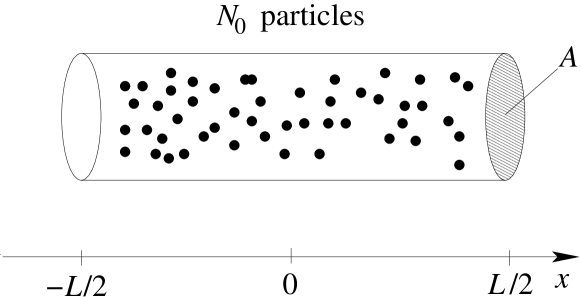
Figure 1: $N_{0}$ particles distributed within a cylinder of section $A$ and length $L$.

II Thermodynamics of conduction

In this Section, a general account of the thermodynamics of conduction is given. We choose the language of continuum physics, where both extensive and associated intensive thermodynamic variables becomes local fields. Although, in view of the applications that follow, we specialize our discussion to diffusion, analogous considerations directly translate to other conduction processes, like e.g. the electric or thermal ones.

II.1 General discussion

Consider a system of $N_{0}$ equal particles confined within a cylinder of section $A$ and radius much smaller than the length $L$ (see Fig. 1). The cylinder is thermally, mechanically, and chemically isolated. In order to simplify the notations, particles are assumed to be uniformly distributed in any cross-section of the cylinder, so that we are basically reduced to a one-dimensional ($1d$) problem. Indicating as $N(x,t)$ the $3d$ particle distribution function, we will be concerned below about its $n$th-order moments:

$$N_{n}\equiv A\;\int\mathrm{d}x\;x^{n}\;N(x,t)\,$$ (1)

(if not otherwise indicated, integrals over $x$ are intended to span the interval $[-L/2,L/2]$). Assuming local equilibrium, we may define a local entropy density $\sigma(N(x,t))$. The system’s (constrained) entropy becomes thus the functional

$$S[N]=A\int\mathrm{d}x\;\sigma(N(x,t)).$$ (2)

A measure about how far the system is from equilibrium is given by the first variation

$$\delta S[N]=-A\int\mathrm{d}x\;\frac{\mu}{T}(N(x,t))\;\delta N(x,t),$$ (3)

where

$$\frac{\mu}{T}(N(x,t))\equiv-\frac{\delta S[N]}{\delta N(x)}=-\frac{\partial\sigma(N(x,t))}{\partial N(x,t)}$$ (4)

is the local intensive parameter associated to the number of particles in the entropy representation of thermodynamics callen_01 , and the variations of the density profile $\delta N(x,t)$ must satisfy the impermeable-walls boundary condition $\delta N_{0}=A\;\int\mathrm{d}x\;\delta N(x,t)=0.$ While the equilibrium distribution $N_{\rm eq}(x)$ could be non-uniform, the extremal requirement of zero first-variation $\delta S[N_{\rm eq}]=0$ implies that at equilibrium $\mu/T$ is the same in any position $x$, as one may verify considering the specific variation reallocating a particle from $x_{1}$ to $x_{2}$, $\delta N(x)=[\delta(x-x_{2})-\delta(x-x_{1})]/A$.

The so-called fluctuation approximation amounts to a Taylor expansion to quadratic order of $S$ around $N_{\rm eq}$:

$$S[N]\simeq S[N_{\rm eq}]+\frac{A}{2}\int\mathrm{d}x\;\left.\frac{\partial^{2}\sigma}{\partial N^{2}}\right|_{N_{\rm eq}(x)}\;\delta N(x,t)^{2}.$$ (5)

The expression of the functional derivative as

$$\frac{\delta S[N]}{\delta N(x)}=\left.\frac{\partial^{2}\sigma}{\partial N^{2}}\right|_{N_{\rm eq}(x)}\;\delta N(x,t)$$ (6)

manifests the (local) generalized force – linear in the fluctuation $\delta N$ with intensity regulated by the thermodynamic response $\partial^{2}\sigma/\partial N^{2}$ – which drives the system back to equilibrium. According to Einstein’s formula einstein_01 ; mauri_01 , the equilibrium probability for a fluctuation is proportional to the exponential of the constrained entropy, implying

$$\mathbb{E}\left[\delta N(x)^{2}\right]=\int\frac{\mathcal{D}(\delta N(x))}{\mathcal{N}}\;\delta N(x)^{2}\exp\left[\frac{A}{2k_{B}}\int\mathrm{d}x\;\left.\frac{\partial^{2}\sigma}{\partial N^{2}}\right|_{N_{\rm eq}(x)}\;\delta N(x)^{2}\right].$$ (7)

A Gaussian integration kardar_01 thus shows that such response is directly linked to the average squared local fluctuation: whence

$$\mathbb{E}\left[\delta N(x)^{2}\right]=-\left[\frac{A\,L}{k_{B}}\left.\frac{\partial^{2}\sigma}{\partial N^{2}}\right|_{N_{\rm eq}(x)}\right]^{-1}.$$ (8)

II.2 Linearly varying intensive parameter

If a system is sufficiently close to equilibrium, even with possibly rough density profiles $N_{\rm eq}(x)$ the intensive parameter $\mu/T$ can be assumed to be spatially smooth (see previous Section). In those cases in which $\mu/T$ is linearly varying along $x$, a number of the above general derivations assume a more transparent meaning.

Since in principle the distribution $N(x,t)$ can be characterized in terms of all its moments $N_{n}$, we may think of the entropy functional as a simple function of such moments attard_01 :

$$S[N]\equiv S(N_{0},N_{1},\ldots).$$ (9)

Retaining only the zero- and first-order moments in the right-hand side and taking the functional derivative, we obtain the equation

$$\;\frac{\delta S[N]}{\delta N(x)} = \frac{\partial S(N_{0},N_{1})}{\partial N_{0}}\;\frac{\delta N_{0}}{\delta N(x)}+\frac{\partial S(N_{0},N_{1})}{\partial N_{1}}\;\frac{\delta N_{1}}{\delta N(x)},$$

$$-\frac{\mu}{T}(x,t) = -\overline{\mu/T}+\frac{\partial S(N_{0},N_{1})}{\partial N_{1}}\;x,$$ (10)

where $\mu/T$ has been regarded directly as a function of $(x,t)$, and $\overline{\mu/T}=\mu/T(0,t)$ is the global intensive parameter. The latter result implies

$$\frac{\partial S(N_{0},N_{1})}{\partial N_{1}}=-\nabla_{x}\frac{\mu}{T}(0,t),$$ (11)

with $\nabla_{x}(\mu/T)$ uniform within this approximation. One thus recognizes that the thermodynamic force restoring the fluctuation to equilibrium is now seen as the gradient in the intensive parameter $\mu/T$. Since, in view of the impermeable boundaries, $N_{0}$ is the same for any distribution, it is not a relevant thermodynamic parameter and may be safely neglected in what follows. Indicating as $N_{1,{\rm eq}}$ the first moment of $N_{\rm eq}$, the fluctuation approximation can now be written as

$$S(N_{1})\simeq S(N_{1,{\rm eq}})+\frac{1}{2}\left.\frac{\partial^{2}S}{\partial N_{1}^{2}}\right|_{N_{1,{\rm eq}}}\;\delta N_{1}^{2}.$$ (12)

The use of the Einstein’s formula einstein_01 ; mauri_01 for the probability of a fluctuation $\delta N_{1}$ gives, for the generalized force,

$$-\nabla_{x}\frac{\mu}{T}(0,t)\simeq\left.\frac{\partial^{2}S}{\partial N_{1}^{2}}\right|_{N_{1,{\rm eq}}}\;\delta N_{1}(t)=-\frac{k_{B}}{\mathbb{E}[\delta N_{1}^{2}]}\;\delta N_{1}(t).$$ (13)

The time derivative of $\delta N_{1}$ is closely related to the number flux $J_{N}$. Take, for simplicity, a quasi-stationary state within the cylinder, i.e., a situation in which the thermodynamic parameters are almost time-independent. A quasi-stationary state can only be supported by the existence of uniform fluxes. In such a way, the number of particles entering arbitrary small volumes in a given time interval is equal to those leaving it. Assuming thus $J_{N}(x,t)=\overline{J}(t)$ for $x\in[-L/2,L/2]$ (slowly varying in $t$), and $J_{N}(x,t)=0$ for $x\notin[-L/2,L/2]$, we have

$$\nabla_{x}J_{N}(x,t)=\overline{J}_{N}(t)\,\left[\delta(x+L/2)-\delta(x-L/2)\right].$$ (14)

Plugging this result in the continuity equation,

$$\partial_{t}\,\delta N(x,t)=\partial_{t}\,N(x,t)=-\nabla_{x}J_{N}(x,t),$$ (15)

we indeed obtain

$$\partial_{t}\,\delta N_{1}(t)=AL\;\overline{J}_{N}(t).$$ (16)

II.3 Onsager regression dynamics

Consider a small fluctuation at time $t_{0}$, which can be monitored through the first moment of the density profile, $\delta N_{1}(t_{0})$. According to Onsager onsager_01 , the thermodynamic force determining the behavior of $\delta N_{1}$ does not depend on whether the fluctuation is spontaneous or generated by the application of an external field or reservoir. It is possible to prove attard_02 that the most likely small-time behavior of $\delta N_{1}(t_{0}+\tau)$, $\overline{\delta N_{1}}(t_{0}+\tau)$, is linear both in the thermodynamic force and in time:

$$\overline{\delta N_{1}}(t_{0}+\tau)\;\begin{subarray}{c}\simeq\\ |\tau|\ll 1\end{subarray}\;\delta N_{1}(t_{0})-|\tau|\;\frac{\Lambda}{2}\;\nabla_{x}\frac{\mu}{T}(0,t_{0}),$$ (17)

where $\Lambda$ is a (positive) coefficient encoding the transport properties of the system (see below). Eq. (17) applies to $|\tau|$ larger than the microscopic (molecular) time-scale of the dynamics, but still small with respect to the significant macroscopic evolution of the system attard_02 . In terms of the number flux, Eq. (17) can be rewritten as

$$\overline{J}_{N}(t_{0}+\tau)\simeq\frac{1}{AL}\;\frac{\overline{\delta N_{1}}(t_{0}+\tau)-\delta N_{1}(t_{0})}{|\tau|}=-\frac{\Lambda}{2AL}\;\nabla_{x}\frac{\mu}{T}(0,t_{0}).$$ (18)

If the intensive parameter $\mu/T$ can be split into chemical potential $\mu$ and temperature $T$, and the latter can be assumed to be uniform along the system, this result is often written as the first Fick’s law fick_01 :

$$\overline{J}_{N}=-D\;\nabla_{x}N,$$ (19)

with

$$D\equiv\frac{\Lambda}{2AL}\;\frac{1}{T}\;\frac{\partial\mu}{\partial N}$$ (20)

the diffusion coefficient.

More generally, the coefficient $\Lambda$ is related to the fluctuation’s autocorrelation by the Green-Kubo relation green_01 ; kubo_01 ; kubo_02 :

$$\Lambda=-\frac{2}{k_{B}\,|\tau|}\left(\mathbb{E}[\delta N_{1}(t_{0}+\tau)\;\delta N_{1}(t_{0})]-\mathbb{E}\left[\delta N_{1}(t_{0})^{2}\right]\right),$$ (21)

where $\mathbb{E}\left[\delta N_{1}(t_{0})^{2}\right]=\mathbb{E}\left[\delta N_{1}^{2}\right]$ is an average over the equilibrium distribution. Equivalently, the system can be characterized in terms of a coefficient $\lambda$ which singles out the dynamical part of the response and is defined as

$$\lambda\equiv\frac{k_{B}\;\Lambda}{\mathbb{E}[\delta N_{1}^{2}]}=-\frac{2}{|\tau|}\frac{\mathbb{E}[\delta N_{1}(t_{0}+\tau)\;\delta N_{1}(t_{0})]-\mathbb{E}\left[\delta N_{1}(t_{0})^{2}\right]}{\mathbb{E}\left[\delta N_{1}(t_{0})^{2}\right]}.$$ (22)

In the case of simple diffusion, in the next Section we will explicitly show how $\lambda$ is related to the local transport coefficient $D$ and to the global geometry of the system. In terms of $\lambda$, Eq. (17) recasts into

$$\overline{\delta N_{1}}(t_{0}+\tau)\;\begin{subarray}{c}\simeq\\ |\tau|\ll 1\end{subarray}\;\delta N_{1}(t_{0})-\frac{\lambda\;|\tau|}{2}\;\delta N_{1}(t_{0}).$$ (23)

At larger $\tau$, for dynamical evolutions both Gaussian and Markovian the Doob’s theorem doob_01 ; doob_02 ensures an exponential decay of the fluctuation given by

$$\overline{\delta N_{1}}(t_{0}+\tau)=\delta N_{1}(t_{0})\;\mathrm{e}^{-\frac{\lambda\,|\tau|}{2}}.$$ (24)

In summary, we can appreciate that the nonequilibrium behavior of a macroscopic observable can be synthesized in terms of a static response coefficient $\mathbb{E}\left[\delta N_{1}^{2}\right]$ determining the strength of the force restoring equilibrium, and of a dynamic response coefficient $\lambda$ describing the time decay of the nonequilibrium fluctuation. Conversely, by monitoring the time evolution of $\overline{\delta N_{1}}(t)$ sensible information about $\lambda$ can be obtained.

III Conduction and Brownian motion

One of the easiest setup in which the previous general nonequilibrium discussion can be tested is perhaps that in which particles are endowed with a Brownian dynamics. The typical situation within this context corresponds to the interaction of the $N_{0}$ particles with an heat bath of smaller ones (e.g., water) at a given temperature. Although the underlying dynamics is assumed to be Hamiltonian, the interaction with the heat bath may be effectively represented by a stochastic term, so that the heat bath particles are not explicitly traced. Implicitly, the motion of the heat bath particles is assumed to compensate that of the Brownian ones, in order to preserve energy and momenta, and to be in conditions of zero convection. In the overdamped regime kardar_01 , the equation of motion for the coordinate $x_{i}$ of each Brownian particle is given by the Langevin stochastic differential equation

$$x_{i}(t+\mathrm{d}t)=x_{i}(t)+\sqrt{2D}\;\mathrm{d}W(t),$$ (25)

where $W(t)$ is a Wiener process doob_02 , and reflecting boundary conditions are applied as $x_{i}=\pm L/2$. In Physics’ literature, Eq. (25) corresponds to a Gaussian white noise evolution for $\mathrm{d}x_{i}/\mathrm{d}t$ kardar_01 .

On the basis of the (Lagrangian) particles coordinates $x_{i}$, the distribution function $N(x,t)$ is defined as

$$N(x,t)\equiv\frac{1}{A}\;\sum_{i=1}^{N}\delta(x-x_{i}(t)),$$ (26)

where $x$ is regarded as an Eulerian coordinate. In the present case, there are two sources of randomness for $N(x,t)$: one is the distribution of the initial conditions $\{x_{i}(t_{0})\}$; the other is because the dynamics itself is a random process. As a consequence of the latter, the most likely time evolution of the distribution function, $\overline{N}(x,t)$, satisfies the Fokker-Planck equation kardar_01

$$\partial_{t}\overline{N}(x,t)=D\;\nabla^{2}_{x}\overline{N}(x,t).$$ (27)

The solution is obtained by applying the appropriate Green function for reflecting boundaries at $x=\pm L/2$ to the initial distribution $N(x_{0},t_{0})$ gardiner_01 :

$$\overline{N}(x,t)=\int\frac{\mathrm{d}x_{0}}{L}\left[1+2\sum_{n=1}^{\infty}{\rm e}^{-\frac{n^{2}\pi^{2}\,D\,(t-t_{0})}{L^{2}}}\cos\left(n\,\pi\,\frac{2x+L}{2L}\right)\cos\left(n\,\pi\,\frac{2x_{0}+L}{2L}\right)\right]N(x_{0},t_{0}).$$ (28)

Independently of $N_{0}$, the equilibrium distribution turns out to be uniform: $N_{\rm eq}(x)=\lim_{t\to+\infty}\overline{N}(x,t)=N_{0}/AL$, and a straightforward calculation yields

$$\overline{\delta N_{1}}(t)=-4AL\sum_{\begin{subarray}{c}n=1\\ n\;\textrm{odd}\end{subarray}}^{+\infty}\frac{{\rm e}^{-\frac{n^{2}\pi^{2}\,D\,(t-t_{0})}{L^{2}}}}{n^{2}\pi^{2}}\int\mathrm{d}x_{0}\;\cos\left(n\,\pi\,\frac{2x_{0}+L}{2L}\right)\;N(x_{0},t_{0}).$$ (29)

If $N(x_{0},t_{0})$ is sufficiently close to $N_{\rm eq}$, Eq. (29) is dominated by the $n=1$ term, and we recover Eq. (24) with

$$\lambda=\frac{2\pi^{2}\,D}{L^{2}}.$$ (30)

As anticipated, we thus see that $\lambda$ is affected by both local transport properties and global aspects of the geometry of the system. In Fig. 2 the numerical simulation of a system of particles described by Eq. (25) is compared with the analytical results.

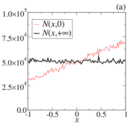
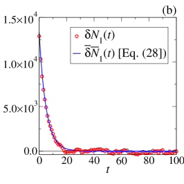
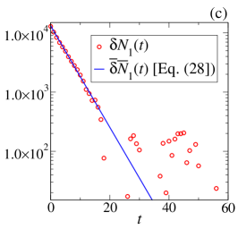
Figure 2: Conduction and Brownian motion (simulation dimensionless units). Eqs. (25) are numerically integrated for $N_{0}=10^{5}$ independent particles with reflecting boundaries at $\pm 1$ ($L=2$) and $D=0.08$. To calculate $N(x,t)$, the interval $[-1,1]$ is coarse grained in $100$ cells; $N(x,0)\equiv(1+a\,L\,x)\,N_{0}/(AL)$, with $x$ indicating the center of the cells and $a=0.2$. (a): Initial and long-term distribution. (b,c): Numerical evaluation of $\delta N_{1}(t)$ (circles) is compared with Eq. (29) (line).

IV Conduction and chaotic dynamics

In this and in the following Section we address the phenomenology of the regression of a nonequilibrium distribution within the context of the logistic map. The basic question we would like to explore is whether some of the general Onsager results do generalize to such a dynamics. Before entering into details, some words of caution are in order. In the case of the logistic map, basic assumptions ordinarily underlying the Onsager discussion are posed into question. First, the logistic map’s dynamics is not local: being conceptually the result of a Poincaré section on an orbit, for the logistic map “$t$” becomes a discrete iteration time and at $t+1$ the iterates are mapped to a space location typically far from that occupied at $t$. Second, the dynamics is inherently non-reversible: the preimage of each iterate at time $t$ corresponds to two distinct points. In view of these remarks, the study of the regression to equilibrium of a quantity as $\overline{\delta N}_{1}(t)$ and its possible relation with local dynamical coefficients – such as the Lyapunov exponent schuster_01 ; beck_01 ; robledo_01 – becomes thus particularly interesting at a fundamental level. In what follows, our aim is to give a first numerical account of such a study, which certainly deserves further insight in the future.

Taking for simplicity $L=2$ (in natural dimensionless units), Eqs. (25) are now replaced by the logistic-map iterations

$$x_{i}(t+1)=1-\mu_{\rm lm}\;x_{i}(t)^{2}\qquad(x_{i}\in[-1,1]).$$ (31)

For each particle, the iterates tend to an attractor whose characteristics depend on the value of the control parameter $0\leq\mu_{\rm lm}\leq 2$. Specifically, with $\mu_{\rm lm}=2$ the attractor’s dynamics is fully chaotic (positive Lyapunov exponent) schuster_01 ; beck_01 ; robledo_01 . Although the dynamics in Eq. (31) is now deterministic, a positive exponential divergence of two initially close initial conditions implies that any randomness in the definition of the initial coordinates results in a random behavior for $N(x,t)$. The latter is again defined as in Eq. (26), with the Lagrangian coordinates $x_{i}(t)$ substituted now by $N_{0}$ independent copies of the logistic map’s coordinates, each evolving through Eq. (31).

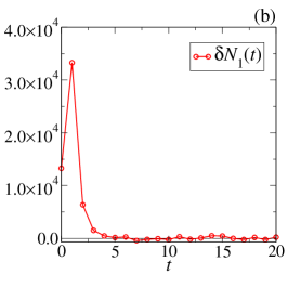
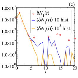
Figure 3: Chaotic conduction. The same numerical analysis displayed in Fig 2 is performed replacing Eqs. (25) with Eqs. (31) and $\mu_{\rm lm}=2$. (a): Plots of the distribution $N(x,t)$ at different time. (b): Numerical evaluation of $\delta N_{1}(t)$ (the line is a guide to the eye). (c) The numerical evaluation of $\delta N_{1}(t)$ for a single history (circles) is compared with averages over many histories (lines).

For the sake of simplicity, in Fig. 3 we consider the same (linear) $N(x,0)$ used for the Wiener process in the previous Section. With a single iteration, the chaotic map quickly drives this initial distribution close to the equilibrium one, $N_{\rm eq}(x)=\lim_{t\to+\infty}\overline{N}(x,t)$; the latter is in this case $x$-dependent with a characteristic “U” shape (see Fig. 3a) schuster_01 ; beck_01 . In parallel, apart from the initial value, the time evolution of $\delta N_{1}(t)$ reported in Fig. 3b displays features of a monotonic decay. The log-linear plot of Fig. 3c, where averages are also taken over different histories sharing the same $N(x,0)$, provides evidence of an exponential decay footnote_1 .

V Conduction at the onset of chaos

At the chaos threshold $\mu_{\rm lm}=1.401155189092\ldots$ (the period-doubling accumulation point schuster_01 ; beck_01 ; robledo_01 ) the Lyapunov exponent collapses to zero and to get sensible information about the microscopic dynamics one is forced to consider an infinite series of specific time-subsequences and to replace exponential divergence (and convergence) with a spectrum of power-laws. Correspondingly, the Lyapunov exponent must be substituted by an infinite series of generalized ones robledo_01 ; baldovin_01 ; mayoral_01 ; fuentes_01 .

Fig. 4 displays the numerical analysis performed starting with the same (linear) $N(x,0)$ of the previous cases, for the logistic map at the onset of chaos $\mu_{\rm lm}=1.401155189092\ldots$. As to be expected, results are now much more involved. In Fig. 4a it is shown that the first iteration sets to zero $N(x,1)$ for $x$ smaller then about $x=-0.5$, in correspondence of the (first) gap formation schuster_01 ; beck_01 ; robledo_01 ; fuentes_01 . Then, the long-time distribution $N(x,t\gg 1)$ reflects the multi-fractal properties of the attractor at the edge of chaos, being characterized by many spikes and gaps. Indeed, initially trajectories are spread out in the interval $[-1,1]$ and, except for the few that are initiated inside the multifractal attractor, they get there via a sequence of gap formations schuster_01 ; beck_01 ; robledo_01 ; fuentes_01 . In practice most of them get into the attractor fairly soon, so, after a few iterations, the first moment is built from positions of the attractor, which are formed by bands (with inner gaps) separated by (main) gaps (see, e.g., Fig. 2 in Ref. fuentes_01 ). This implies $N(x,t)\simeq 0$ for $x$ not in the attractor, if $t$ is sufficiently large.

A careful comparison of Fig. 4a with Fig. 4d also reveals that in the present case it is not sufficient to take the long-time limit of $N(x,t)$ to get the (invariant) equilibrium distribution, since sensible differences can be appreciated, e.g., between $N(x,2^{10})$ and $N(x,2^{10}+1)$. With this in mind, our numerical study proceeds defining

$$\delta N_{1}(t)\equiv A\;\int\mathrm{d}x\;x\;\left[N(x,t)-N(x,\overline{t})\right],$$ (32)

with $\overline{t}=2^{10}$ (Figs. 4b and 4c) and $\overline{t}=2^{10}+1$ (Figs. 4e and 4f). Specifically, in Figs. 4b and 4e we see that in both cases $\delta N_{1}(t)$ has an oscillating behavior in which even and odd time iterations are well separated. For further specific time subsequences, the log-log plots of $|\delta N_{1}(t)|$ in Figs. 4c and 4f may recall power-law behaviors reminiscent to those characterizing the generalized Lyapunov spectrum baldovin_01 ; mayoral_01 , although deeper insight is certainly needed to get definite results.

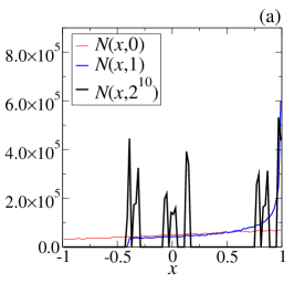
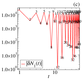
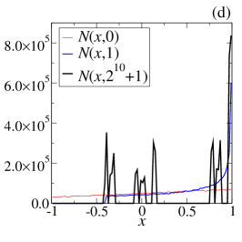
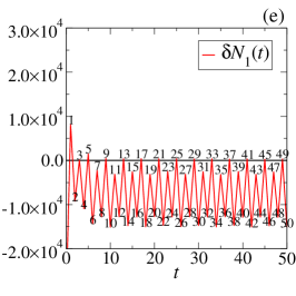
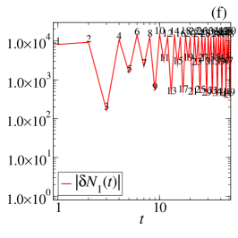
Figure 4: Conduction at the onset of chaos. The numerical analysis is performed with Eqs. (31) and $\mu_{\rm lm}=1.401155189092\ldots$. (a,d): Plots of the distribution $N(x,t)$ at different time. (b,e): Numerical evaluation of $\delta N_{1}(t)$ defined through Eq. (32) with $\overline{t}=2^{10}$ in (b) and $\overline{t}=2^{10}+1$ in (e) (the line is a guide to the eye). (c,f) Same as (b,e), in log-log scale.

VI Conclusions and perspectives

In this paper we studied the relaxation process of a nonequilibrium fluctuation in a context in which the particles’ dynamics is described by logistic map iterations. This allowed us to explore whether some of the features of the classic Onsager’s regression description generalize to non-local, non-reversible microscopic dynamics.

After a general discussion of conductive processes in which simple thermodynamic observables have been introduced, the conventional example of Browninan particles has been analytically and numerically worked out. In this way, contact has been established among the underlying dynamics and system’s geometry, and the thermodynamic behavior.

Substituting the Brownian dynamics with logistic map iterations, we numerically analyzed the same relaxation process. While evidence of a monotonic relaxation has been found when the control parameter $\mu_{\rm lm}$ is tuned to chaoticity footnote_2 , at the onset of chaos a much more involved dynamical picture emerges, which may be rationalized in terms of specific time subsequences. Clarification of the latter result demands for a better construction of the invariant (equilibrium) measure than the one obtained by simply taking the long-time limit of the particles’ distribution. More generally, a statistical mechanics approach diaz_01 linking the microscopic dynamics (e.g., in terms of the Lyapunov or generalized Lyapunov exponents) to the observed nonequilibrium thermodynamics is an intriguing open question.

References

- (1) P. Hertel, Continuum Physics, (Springer-Verlag Berlin Heidelberg 2012).
- (2) L. Onsager, Phys. Rev. 37, (1931) 405; 38, (1931) 2265.
- (3) H.G. Schuster, Deterministic Chaos: An Introduction, (2nd ed.; VCH Publishers: Weinheim, Germany, 1988).
- (4) C. Beck, F. Schlogl, Thermodynamics of Chaotic Systems, (Cambridge University Press: Cambridge, UK, 1993).
- (5) A. Robledo, Entropy 15, (2013) 5178.
- (6) H. B. Callen, Thermodynamics and an Introduction to Thermostatistics, (2nd edition, Wiley, New York 1985).
- (7) A. Einstein, Ann. d. Physik 33, (1910) 1275.
- (8) R. Mauri, Non-Equilibrium Thermodynamics in Multiphase Flows, (Springer, Dordrecht 2013).
- (9) M. Kardar, Statistical Physics of Fields, (Cambridge University Press, New York 2007).
- (10) P. Attard, J. Chem. Phys. 121, (2004) 7076.
- (11) P. Attard, J. Chem. Phys. 122, (2005) 154101.
- (12) A. Fick, Poggendorffs Annalen. 94, (1855) 59, reprinted in Journal of Membrane Science 100, (1995) 33.
- (13) M.S. Green, J. Chem. Phys. 22, (1954) 398.
- (14) R. Kubo, Rep. Progr. Phys. 29, (1966) 255.
- (15) R. Kubo, R, M. Toda, and N. Hashitsume, Statistical Physics II. Non-equilibrium Statistical Mechanics, (Springer-Verlag, Berlin 1978).
- (16) J.L. Doob, Ann. Math. 43, (1942) 351.
- (17) J.L. Doob, Stochastic processes (Wiley, New York 1953).
- (18) C.W. Gardiner, Handbook of Stochastic Methods, (3rd ed. Springer-Verlag Berlin Heidelberg 2004)
- (19) F. Baldovin, A. Robledo, Phys. Rev. E 69, (2004) 045202.
- (20) E. Mayoral, A. Robledo, Phys. Rev. E 72, (2005) 026209.
- (21) M.A. Fuentes, A. Robledo, J. Stat. Mech. P01001 (2010).
- (22) A. Díaz-Ruelas, A. Robledo Eur. Phys. Lett. 105, 40004 (2014).
- (23) Added Note. After the manuscript has been accepted, correspondence with A. Díaz-Ruelas and A. Robledo pointed out that even in the chaotic case the regression to equilibrium may involve non-monotonic power-law patterns. The exponential decay reported in Fig. 3c may be due to the coincidence of the average procedure over the initial distributions with a scarce cell-resolution (100 cells for the plotted results).
- (24) See, however, note footnote_1 .