Sparse Depth Sensing for Resource-Constrained Robots

Abstract

We consider the case in which a robot has to navigate in an unknown environment but does not have enough on-board power or payload to carry a traditional depth sensor (e.g., a 3D lidar) and thus can only acquire a few (point-wise) depth measurements. We address the following question: is it possible to reconstruct the geometry of an unknown environment using sparse and incomplete depth measurements? Reconstruction from incomplete data is not possible in general, but when the robot operates in man-made environments, the depth exhibits some regularity (e.g., many planar surfaces with only a few edges); we leverage this regularity to infer depth from a small number of measurements. Our first contribution is a formulation of the depth reconstruction problem that bridges robot perception with the compressive sensing literature in signal processing. The second contribution includes a set of formal results that ascertain the exactness and stability of the depth reconstruction in 2D and 3D problems, and completely characterize the geometry of the profiles that we can reconstruct. Our third contribution is a set of practical algorithms for depth reconstruction: our formulation directly translates into algorithms for depth estimation based on convex programming. In real-world problems, these convex programs are very large and general-purpose solvers are relatively slow. For this reason, we discuss ad-hoc solvers that enable fast depth reconstruction in real problems. The last contribution is an extensive experimental evaluation in 2D and 3D problems, including Monte Carlo runs on simulated instances and testing on multiple real datasets. Empirical results confirm that the proposed approach ensures accurate depth reconstruction, outperforms interpolation-based strategies, and performs well even when the assumption of structured environment is violated.

Supplemental Material

• Video demonstrations:
  https://youtu.be/vE56akCGeJQ

• Source code:
  https://github.com/sparse-depth-sensing

I Introduction

Recent years have witnessed a growing interest towards miniaturized robots, for instance the RoboBee [1], Piccolissimo [2], the DelFly [3, 4], the Black Hornet Nano [5], Salto [6]. These robots are usually palm-sized (or even smaller), can be deployed in large volumes, and provide a new perspective on societally relevant applications, including artificial pollination, environmental monitoring, and disaster response. Despite the rapid development and recent success in control, actuation, and manufacturing of miniature robots, on-board sensing and perception capabilities for such robots remain a relatively unexplored, challenging open problem. These small platforms have extremely limited payload, power, and on-board computational resources, thus preventing the use of standard sensing and computation paradigms.

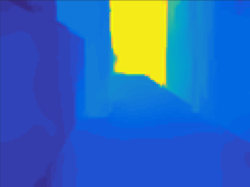
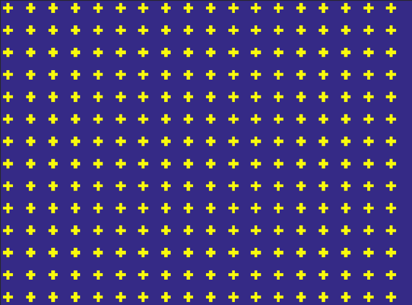
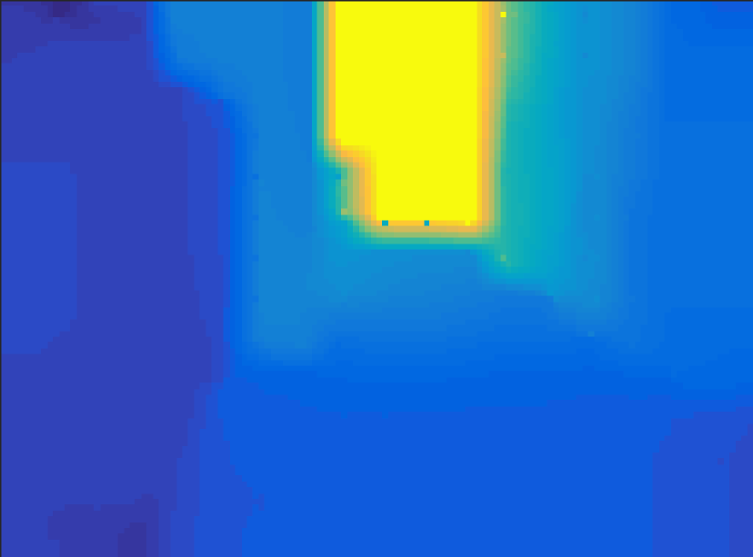
(a) ground truth	(b) 2% grid samples	(c) reconstruction
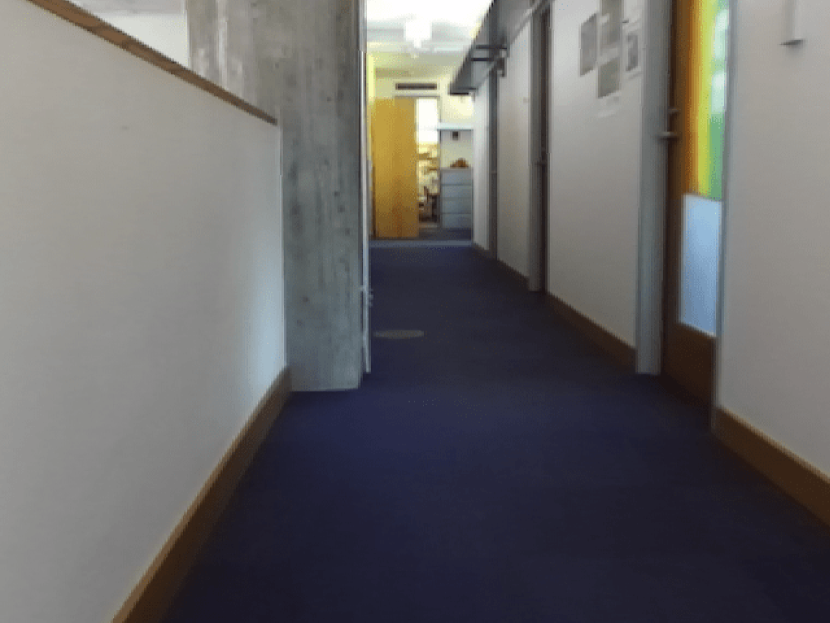
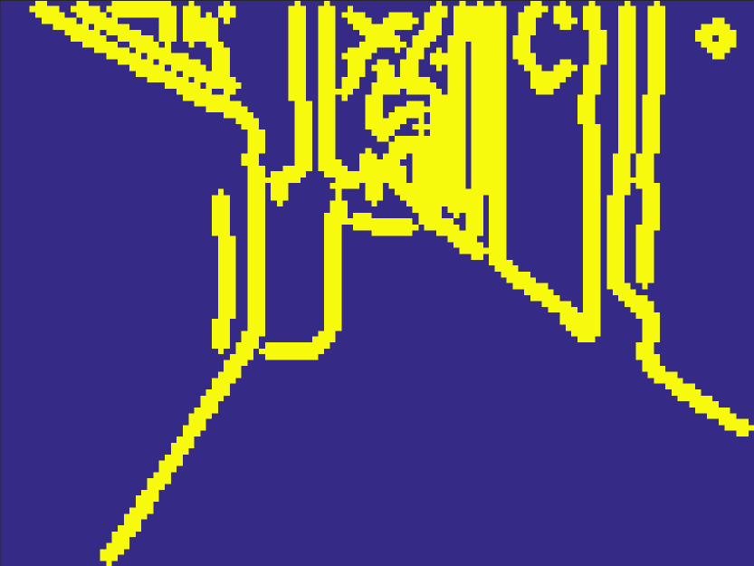
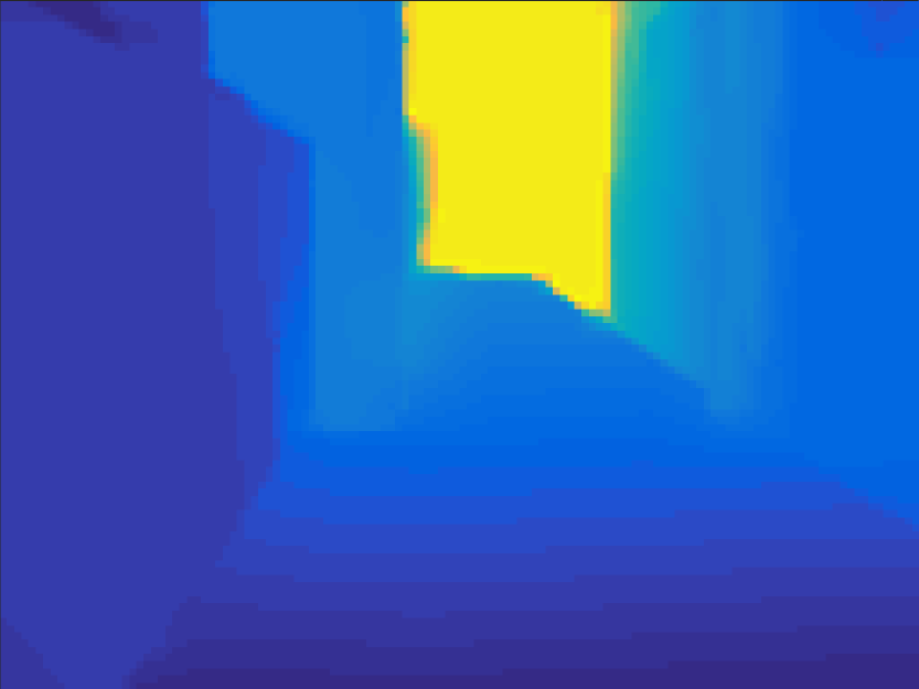
(d) RGB image	(e) sample along edges	(f) reconstruction

Figure 1: We show how to reconstruct an unknown depth profile (a) from a handful of samples (b). Our reconstruction is shown in (c). Our results also apply to traditional stereo vision and enable accurate reconstruction (f) from few depth measurements (e) corresponding to the edges in the RBG image (d). Figures (a) and (d) are obtained from a ZED stereo camera.

In this paper we explore novel sensing techniques for miniaturized robots that cannot carry standard sensors. In the last two decades, a large body of robotics research focused on the development of techniques to perform inference from data produced by “information-rich” sensors (e.g., high-resolution cameras, 2D and 3D laser scanners). A variety of approaches has been proposed to perform geometric reconstruction using these sensors, for instance see [7, 8, 9] and the references therein. On the other extreme of the sensor spectrum, applications and theories have been developed to cope with the case of minimalistic sensing [10, 11, 12, 13]. In this latter case, the sensor data is usually not metric (i.e., the sensor cannot measure distances or angles) but instead binary in nature (e.g., binary detection of landmarks), and the goal is to infer only the topology of the (usually planar) environment rather than its geometry. This work studies a relatively unexplored region between these two extremes of the sensor spectrum.

Our goal is to design algorithms (and lay the theoretical foundations) to reconstruct a depth profile (i.e., a laser scan in 2D, or a depth image in 3D, see Fig. 1) from sparse and incomplete depth measurements. Contrary to the literature on minimalistic sensing, we provide tools to recover complete geometric information, while requiring much fewer data points compared to standard information-rich sensors. This effort complements recent work on hardware and sensor design, including the development of lightweight, small-sized depth sensors. For instance, a number of ultra-tiny laser range sensors are being developed as research prototypes (e.g., the dime-sized, 20-gram laser of [14], and an even smaller lidar-on-a-chip system with no moving parts [15]), while some other distance sensors have already been released to the market (e.g., the TeraRanger’s single-beam, 8-gram distance sensor [16], and the LeddarVu’s 8-beam, 100-gram laser scanner [17]). These sensors provide potential hardware solutions for sensing on micro (or even nano) robots. Although these sensors meet the requirements of payload and power consumption of miniature robots, they only provide very sparse and incomplete depth data, in the sense that the raw depth measurements are extremely low-resolution (or even provide only a few beams). In other words, the output of these sensors cannot be utilized directly in high-level tasks (e.g., object recognition and mapping), and the need to reconstruct a complete depth profile from such sparse data arises.

Contribution. We address the following question: is it possible to reconstruct a complete depth profile from sparse and incomplete depth samples? In general, the answer is negative, since the environment can be very adversarial (e.g., 2D laser scan where each beam is drawn randomly from a uniform distribution), and it is impossible to recover the depth from a small set of measurements. However, when the robot operates in structured environments (e.g., indoor, urban scenarios) the depth data exhibits some regularity. For instance, man-made environments are characterized by the presence of many planar surfaces and a few edges and corners. This work shows how to leverage this regularity to recover a depth profile from a handful of sensor measurements. Our overarching goal is two-fold: to establish theoretical conditions under which depth reconstruction from sparse and incomplete measurements is possible, and to develop practical inference algorithms for depth estimation.

Our first contribution, presented in Section IV, is a general formulation of the depth estimation problem. Here we recognize that the “regularity” of a depth profile is captured by a specific function (the $\ell_{0}$-norm of the 2^nd-order differences of the depth profile). We also show that by relaxing the $\ell_{0}$-norm to the (convex) $\ell_{1}$-norm, our problem falls within the cosparsity model in compressive sensing (CS). We review related work and give preliminaries on CS in Section II and Section III.

The second contribution, presented in Section V, is the derivation of theoretical conditions for depth recovery. In particular, we provide conditions under which reconstruction of a profile from incomplete measurements is possible, investigate the robustness of depth reconstruction in the presence of noise, and provide bounds on the reconstruction error. Contrary to the existing literature in CS, our conditions are geometric (rather than algebraic) and provide actionable information to guide sampling strategy.

Our third contribution, presented in Section VI, is algorithmic. We discuss practical algorithms for depth reconstruction, including different variants of the proposed optimization-based formulation, and solvers that enable fast depth recovery. In particular, we discuss the application of a state-of-the-art solver for non-smooth convex programming, called NESTA [18].

Our fourth contribution, presented in Section VII, is an extensive experimental evaluation, including Monte Carlo runs on simulated data and testing with real sensors. The experiments confirm our theoretical findings and show that our depth reconstruction approach is extremely resilient to noise and works well even when the regularity assumptions are partially violated. We discuss many applications for the proposed approach. Besides our motivating scenario of navigation with miniaturized robots, our approach finds application in several endeavors, including data compression and super-resolution depth estimation.

Section VIII draws conclusions and discusses future research. Proofs and extra visualizations are given in the appendix.

This paper extend the preliminary results presented in [19] in multiple directions. In particular, the error bounds in Section V-B and Section V-C, the algorithms and solvers in Section VI, and most of the experiments of Section VII are novel and have not been previously published.

II Related Work

This work intersects several lines of research across fields.

Minimalistic Sensing. Our study of depth reconstruction from sparse sensor data is related to the literature on minimalistic sensing. Early work on minimalistic sensing includes contributions on sensor-less manipulation [20], robot sensor design [21, 22], and target tracking [23]. [10], [11]. [24] use binary measurements of the presence of landmarks to infer the topology of the environment. [25, 26] reconstruct the topology of a sensor network from unlabeled observations from a mobile robot. [27] and [28] investigate a localization problem using contact sensors. [29] use depth discontinuities measurements to support exploration and search in unknown environments. [30, 13] propose a combinatorial filter to estimate the path (up to homotopy class) of a robot from binary detections. [31] addresses minimality of information for vision-based place recognition.

Sensing and perception on miniaturized robots. A fairly recent body of work in robotics focuses on miniaturized robots and draws inspiration from small animals and insects. Most of the existing literature focuses on the control of such robots, either open-loop or based on information from external infrastructures. However, there has been relatively little work on onboard sensing and perception. For example, the Black Hornet Nano [5] is a military-grade micro aerial vehicle equipped with three cameras but with basically no autonomy. Salto [6] is Berkeley’s 100g legged robot with agile jumping skills. The jump behavior is open-loop due to lack of sensing capabilities, and the motion is controlled by a remote laptop. The RoboBee [1] is an 80-milligram, insect-scale robot capable of hovering motion. The state estimation relies on an external array of cameras. Piccolissimo [2] is a tiny, self-powered drone with only two moving parts, completely controlled by an external, hand-held infrared device. The DelFly Explorer [3, 4] is a 20-gram flying robot with an onboard stereo vision system. It is capable of producing a coarse depth image at 11Hz and is thus one of the first examples of miniaturized flying robot with basic obstacle avoidance capabilities.

Fast Perception and Dense 3D Reconstruction. The idea of leveraging priors on the structure of the environment to improve or enable geometry estimation has been investigated in early work in computer vision for single-view 3D reconstruction and feature matching [32, 33]. Early work by [34] addresses Structure from Motion by assuming the environment to be piecewise planar. More recently, [35] propose an approach to speed-up stereo reconstruction by computing the disparity at a small set of pixels and considering the environment to be piecewise planar elsewhere. [36] combine live dense reconstruction with shape-priors-based 3D tracking and reconstruction. [37] propose a regularization based on the structure tensor to better capture the local geometry of images. [38] produce high-resolution depth maps from subsampled depth measurements by using segmentation based on both RGB images and depth samples. [39] compute a dense depth map from a sparse point cloud. This work is related to our proposal with three main differences. First, the work [39] uses an energy minimization approach that requires parameter tuning (the authors use Bayesian optimization to learn such parameter); our approach is parameter free and only assumes bounded noise. Second, we use a 2^nd-order difference operator to promote depth regularity, while [39] considers alternative costs, including nonconvex regularizers. Finally, by recognizing connections with the cosparsity model in CS, we provide theoretical foundations for the reconstruction problem.

Map Compression. Our approach is also motivated by the recent interest in map compression. [40] propose a compression method for occupancy grid maps, based on the information bottleneck theory. [41, 42] use Gaussian processes to improve 2D mapping quality from smaller amount of laser data. [43] investigate wavelet-based compression techniques for 3D point clouds. [44, 45] discuss point cloud compression techniques based on sparse coding. [46, 47] propose a variable selection method to retain only an important subset of measurements during map building.

Compressive Sensing (CS). Finally, our work is related to the literature on compressive sensing [48, 49, 50, 51]. While Shannon’s theorem states that to reconstruct a signal (e.g., a depth profile) we need a sampling rate (e.g., the spatial resolution of our sensor) which must be at least twice the maximum frequency of the signal, CS revolutionized signal processing by showing that a signal can be reconstructed from a much smaller set of samples if it is sparse in some domain. CS mainly invokes two principles. First, by inserting randomness in the data acquisition, one can improve reconstruction. Second, one can use $\ell_{1}$-minimization to encourage sparsity of the reconstructed signal. Since its emergence, CS impacted many research areas, including image processing (e.g., inpainting [52], total variation minimization [53]), data compression and 3D reconstruction [54, 55, 56], tactile sensor data acquisition [57], inverse problems and regularization [58], matrix completion [59], and single-pixel imaging techniques [60, 61, 62]. While most CS literature assumes that the original signal $z$ is sparse in a particular domain, i.e., $z=Dx$ for some matrix $D$ and a sparse vector $x$ (this setup is usually called the synthesis model), very recent work considers the case in which the signal becomes sparse after a transformation is applied (i.e., given a matrix $D$, the vector $Dz$ is sparse). The latter setup is called the analysis (or cosparsity) model [63, 64]. An important application of the analysis model in compressive sensing is total variation minimization, which is ubiquitous in image processing [53, 65]. In a hindsight we generalize total variation (which applies to piecewise constant signals) to piecewise linear functions.

Depth Estimation from Sparse Measurements. Few recent papers investigate the problem of reconstructing a dense depth image from sparse measurements. [66] exploit the sparsity of the disparity maps in the Wavelet domain. The dense reconstruction problem is then posed as an optimization problem that simultaneously seeks a sparse coefficient vector in the Wavelet domain while preserving image smoothness. They also introduce a conjugate subgradient method for the resulting large-scale optimization problem. Liu et al. [67] empirically show that a combined dictionary of wavelets and contourlets produces a better sparse representation of disparity maps, leading to more accurate reconstruction. In comparison with [66, 67], our work has four major advantages. Firstly, our algorithm works with a remarkably small number of samples (e.g. 0.5%), while both [66, 67] operate with at least 5% samples, depending on the image resolution. Secondly, our algorithm significantly outperforms previous work in both reconstruction accuracy and computation time, hence pushing the boundary of achievable performance in depth reconstruction from sparse measurements. An extensive experimental comparison is presented in Section VII-C3. Thirdly, the sparse representation presented in this work is specifically designed to encode depth profiles, while both [66, 67] use wavelet representations, which do not explicitly leverage the geometry of the problem. Indeed, our representation is derived from a simple, intuitive geometric model and thus has clear physical interpretation. Lastly, unlike previous work which are mostly algorithmic in nature, we provide theoretical guarantees and error bounds, as well as conditions under which the reconstruction is possible.

III Preliminaries and Notation

We use uppercase letters for matrices, e.g., $D\in{{\mathbb{R}}^{p\times n}}$, and lowercase letters for vectors and scalars, e.g, $z\in{{\mathbb{R}}^{n}}$ and $a\in{{\mathbb{R}}}$. Sets are denoted with calligraphic fonts, e.g., ${\cal M}$. The cardinality of a set ${\cal M}$ is denoted with $|{\cal M}|$. For a set ${\cal M}$, the symbol $\overline{{\cal M}}$ denotes its complement. For a vector $z\in{{\mathbb{R}}^{n}}$ and a set of indices ${\cal M}\subseteq\{1,\ldots,n\}$, $z_{\cal M}$ is the sub-vector of $z$ corresponding to the entries of $z$ with indices in ${\cal M}$. In particular, $z_{i}$ is the $i$-th entry. The symbols ${\mathbf{1}}$ (resp. ${\mathbf{0}}$) denote a vector of all ones (resp. zeros) of suitable dimension.

The support set of a vector is denoted with

$$\mathrm{supp}(z)=\{i\in\{1,\dots,n\}\;{:}\;z_{i}\neq 0\}.$$

We denote with $\|z\|_{2}$ the Euclidean norm and we also use the following norms:

$$\|z\|_{\infty} \doteq \max_{i=1,\ldots,n}\;|z_{i}|\quad\text{($\ell_{\infty}$ norm)}$$ (1)

$$\|z\|_{1} \doteq \sum_{i=1,\ldots,n}|z_{i}|\quad\text{($\ell_{1}$ norm)}$$ (2)

$$\|z\|_{0} \doteq |\mathrm{supp}(z)|\quad\text{($\ell_{0}$ pseudo-norm)}$$ (3)

Note that $\|z\|_{0}$ is simply the number of nonzero elements in $z$. The sign vector $\text{sign}(z)$ of $z\in\mathbb{R}^{n}$ is a vector with entries:

$$\text{sign}(z)_{i}\doteq\left\{\begin{array}[]{ll}+1&\text{if }z_{i}>0\\ \;\;\;0&\text{if }z_{i}=0\\ -1&\text{if }z_{i}<0\end{array}\right.$$

For a matrix $D$ and an index set ${\cal M}$, let $D_{\cal M}$ denote the sub-matrix of $D$ containing only the rows of $D$ with indices in ${\cal M}$; in particular, $D_{i}$ is the $i$-th row of $D$. Similarly, given two index sets ${\cal I}$ and ${\cal J}$, let $D_{{\cal I},{\cal J}}$ denote the sub-matrix of $D$ including only rows in ${\cal I}$ and columns in ${\cal J}$. Let ${\mathbf{I}}$ denote the identity matrix. Given a matrix $D\in{{\mathbb{R}}^{p\times n}}$, we define the following matrix operator norm

$$\|D\|_{\infty\rightarrow\infty}\doteq\max_{i=1,\ldots,p}\|D_{i}\|_{1}.$$

In the rest of the paper we use the cosparsity model in CS. In particular, we assume that the signal of interest is sparse under the application of an analysis operator. The following definitions formalize this concept.

Definition 1 (Cosparsity).

A vector $z\in{{\mathbb{R}}^{n}}$ is said to be cosparse with respect to a matrix $D\in{{\mathbb{R}}^{p\times n}}$ if $\|Dz\|_{0}\ll p$.

Definition 2 ($D$-support and $D$-cosupport).

Given a vector $z\in{{\mathbb{R}}^{n}}$ and a matrix $D\in{{\mathbb{R}}^{p\times n}}$, the $D$-support of $z$ is the set of indices corresponding to the nonzero entries of $Dz$, i.e., ${\cal I}=\mathrm{supp}(Dz)$. The $D$-cosupport ${\cal J}$ is the complement of ${\cal I}$, i.e., the indices of the zero entries of $Dz$.

IV Problem Formulation

Our goal is to reconstruct 2D depth profiles (i.e., a scan from a 2D laser range finder) and 3D depth profiles (e.g., a depth image produced by a kinect or a stereo camera) from partial and incomplete depth measurements. In this section we formalize the depth reconstruction problem, by first considering the 2D and the 3D cases separately, and then reconciling them under a unified framework.

IV-A 2D Depth Reconstruction

In this section we discuss how to recover a 2D depth profile $z^{\diamond}\in{{\mathbb{R}}^{n}}$. One can imagine that the vector $z^{\diamond}$ includes (unknown) depth measurements at discrete angles; this is what a standard planar range finder would measure.

In our problem, due to sensing constraints, we do not have direct access to $z^{\diamond}$, and we only observe a subset of its entries. In particular, we measure

$$y=Az^{\diamond}+\eta\qquad\text{(sparse measurements)}$$ (4)

where the matrix $A\in{{\mathbb{R}}^{m\times n}}$ with $m\ll n$ is the measurement matrix, and $\eta$ represents measurement noise. The structure of $A$ is formalized in the following definition.

Definition 3 (Sample set and sparse sampling matrix).

A sample set ${\cal M}\subseteq\{1,\ldots,n\}$ is the set of entries of the profile that are measured. A matrix $A\in{{\mathbb{R}}^{m\times n}}$ is called a (sparse) sampling matrix (with sample set ${\cal M}$), if $A={\mathbf{I}}_{\cal M}$.

Recall that ${\mathbf{I}}_{\cal M}$ is a sub-matrix of the identity matrix, with only rows of indices in ${\cal M}$. It follows that $Az=z_{\cal M}$, i.e., the matrix $A$ selects a subset of entries from $z$. Since $m\ll n$, we have much fewer measurements than unknowns. Consequently, $z^{\diamond}$ cannot be recovered from $y$, without further assumptions.

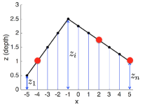
(a)

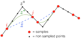
(b)

Figure 2: (a) Example of 2D depth profile. Our goal is to reconstruct the full profile (black solid line) from sparse samples (red dots); (b) When we do not sample the corners and the neighboring points, ($\text{L1}_{D}$) admits multiple minimizers, which obey the conditions of Proposition 14.

In this paper we assume that the profile $z^{\diamond}$ is sufficiently regular, in the sense that it contains only a few “corners”, e.g., Fig. 2(a). Corners are produced by changes of slope: considering 3 consecutive points at coordinates $(x_{i-1},z_{i-1})$, $(x_{i},z_{i})$, and $(x_{i+1},z_{i+1})$, there is a corner at $i$ if

$$\frac{z_{i+1}-z_{i}}{x_{i+1}-x_{i}}-\frac{z_{i}-z_{i-1}}{x_{i}-x_{i-1}}\neq 0.$$ (5)

In the following we assume that $x_{i}-x_{i-1}=1$ for all $i$: this comes without loss of generality since the full profile is unknown and we can reconstruct it at arbitrary resolution (i.e., at arbitrary $x$); hence (5) simplifies to $z_{i-1}-2z_{i}+z_{i+1}\neq 0$. We formalize the definition of “corner” as follows.

Definition 4 (Corner set).

Given a 2D depth profile $z\in{{\mathbb{R}}^{n}}$, the corner set ${\cal C}\subseteq\{2,\ldots,n-1\}$ is the set of indices $i$ such that $z_{i-1}-2z_{i}+z_{i+1}\neq 0$.

Intuitively, $z_{i-1}-2z_{i}+z_{i+1}$ is the discrete equivalent of the 2^nd-order derivative at $z_{i}$. We call $z_{i-1}-2z_{i}+z_{i+1}$ the curvature at sample $i$: if this quantity is zero, the neighborhood of $i$ is flat (the three points are collinear); if it is negative, the curve is locally concave; if it is positive, it is locally convex. To make notation more compact, we introduce the 2^nd-order difference operator:

$$D\doteq\left[\begin{array}[]{cccccc}1&-2&1&0&\ldots&0\\ 0&1&-2&1&\ldots&0\\ \vdots&0&\ddots&\ddots&\ddots&0\\ 0&\ldots&0&1&-2&1\\ \end{array}\right]\in{{\mathbb{R}}^{(n-2)\times n}}$$ (6)

Then a profile with only a few corners is one where $Dz^{\diamond}$ is sparse. In fact, the $\ell_{0}$-norm of $Dz^{\diamond}$ counts exactly the number of corners of a profile:

$$\|Dz^{\diamond}\|_{0}=|{\cal C}|\qquad\text{(\# of corners)}$$ (7)

where $|{\cal C}|$ is the number of corners in the profile.

When operating in indoor environments, it is reasonable to assume that $z^{\diamond}$ has only a few corners. Therefore, we want to exploit this regularity assumption and the partial measurements $y$ in (4) to reconstruct $z^{\diamond}$. Let us start from the noiseless case in which $\eta={\mathbf{0}}$ in (4). In this case, a reasonable way to reconstruct the profile $z^{\diamond}$ is to solve the following optimization problem:

$$\min_{z}\;\|Dz\|_{0}\quad\text{ subject to }Az=y$$ (L0)

which seeks the profile $z$ that is consistent with the measurements (4) and contains the smallest number of corners. Unfortunately, problem (L0) is NP-hard due to the nonconvexity of the $\ell_{0}$ (pseudo) norm. In this work we study the following relaxation of problem (L0):

$$\min_{z}\;\|Dz\|_{1}\quad\text{ subject to }Az=y \text{L1}_{D}$$ ()

which is a convex program (it can be indeed rephrased as a linear program), and can be solved efficiently in practice. Section V provides conditions under which ($\text{L1}_{D}$) recovers the solution of (L0). Problem ($\text{L1}_{D}$) falls in the class of the cosparsity models in CS [64].

In the presence of bounded measurement noise (4), i.e., $\|\eta\|_{\infty}\leq\varepsilon$, the $\ell_{1}$-minimization problem becomes:

$$\min_{z}\;\|Dz\|_{1}\quad\text{ subject to }\;\|Az-y\|_{\infty}\leq\varepsilon \text{L1}_{D}^{\varepsilon}$$ ()

Note that we assume that the $\ell_{\infty}$ norm of the noise $\eta$ is bounded, since this naturally reflects the sensor model in our robotic applications (i.e., bounded error in each laser beam). On the other hand, most CS literature considers the $\ell_{2}$ norm of the error to be bounded and thus obtains an optimization problem with the $\ell_{2}$ norm in the constraint. The use of the $\ell_{\infty}$ norm as a constraint in ($\text{L1}_{D}^{\varepsilon}$) resembles the Dantzig selector of Candes and Tao [68], with the main difference being the presence of the matrix $D$ in the objective.

IV-B 3D Depth Reconstruction

In this section we discuss how to recover a 3D depth profile $Z^{\diamond}\in\mathbb{R}^{r\times c}$ (a depth map, as the one in Fig. 1(a)), using incomplete measurements. As in the 2D setup, we do not have direct access to $Z^{\diamond}$, but instead only have access to $m\ll r\times c$ point-wise measurements in the form:

$$y_{i,j}=Z^{\diamond}_{i,j}+\eta_{i,j}$$ (8)

where $\eta_{i,j}\in{{\mathbb{R}}}$ represents measurement noise. Each measurement is a noisy sample of the depth of $Z^{\diamond}$ at pixel $(i,j)$.

We assume that $Z^{\diamond}$ is sufficiently regular, which intuitively means that the depth profile contains mostly planar regions and only a few “edges”. We define the edges as follows.

Definition 5 (Edge set).

Given a 3D profile $Z\in{{\mathbb{R}}^{r\times c}}$, the vertical edge set ${\cal E}_{V}\subseteq\{2,\ldots,r-1\}\times\{1,\ldots,c\}$ is the set of indices $(i,j)$ such that $Z_{i-1,j}-2Z_{i,j}+Z_{i+1,j}\neq 0$. The horizontal edge set ${\cal E}_{H}\subseteq\{1,\ldots,r\}\times\{2,\ldots,c-1\}$ is the set of indices $(i,j)$ such that $Z_{i,j-1}-2Z_{i,j}+Z_{i,j+1}\neq 0$. The edge set ${\cal E}$ is the union of the two sets: ${\cal E}\doteq{\cal E}_{V}\cup{\cal E}_{H}$.

Intuitively, $(i,j)$ is not in the edge set ${\cal E}$ if the $3\times 3$ patch centered at $(i,j)$ is planar, while $(i,j)\in{\cal E}$ otherwise. As in the 2D case we introduce 2^nd-order difference operators $D_{V}$ and $D_{H}$ to compute the vertical differences $Z_{i,j-1}-2Z_{i,j}+Z_{i,j+1}$ and the horizontal differences $Z_{i-1,j}-2Z_{i,j}+Z_{i+1,j}$:

$$D_{V}Z^{\diamond}\in{{\mathbb{R}}^{(r-2)\times c}},\qquad Z^{\diamond}D_{H}^{\mathsf{T}}\in{{\mathbb{R}}^{r\times(c-2)}}$$ (9)

where the matrices $D_{V}$ and $D_{H}$ are the same as the one defined (6), but with suitable dimensions; each entry of the matrix $D_{V}Z^{\diamond}$ contains the vertical (2^nd-order) differences at a pixel, while $Z^{\diamond}D_{H}^{\mathsf{T}}$ collects the horizontal differences.

Following the same reasoning of the 2D case, we obtain the following $\ell_{1}$-norm minimization

$$\min_{Z} \|\,\text{vec}{\left(D_{V}Z\right)}\|_{1}+\|\,\text{vec}{\left(ZD_{H}^{\mathsf{T}}\right)}\|_{1}$$ (10)

subject to $$Z_{i,j}=y_{i,j}\quad\text{for each measured pixel }(i,j)$$

where $\,\text{vec}{\left(\cdot\right)}$ denotes the (column-wise) vectorization of a matrix, and we assume noiseless measurements. In the presence of measurement noise, the equality constraint in (10) is again replaced by $|Z_{i,j}-y_{i,j}|\leq\varepsilon$, $\forall(i,j)$, where $\varepsilon$ is an upper bound on the pixel-wise noise $\eta_{i,j}$.

IV-C Reconciling 2D and 3D Depth Reconstruction

In this section we show that the 3D depth reconstruction problem (10) can be reformulated to be closer to its 2D counterpart ($\text{L1}_{D}$), if we vectorize the depth profile (matrix $Z$). For a given profile $Z\in{{\mathbb{R}}^{r\times c}}$, we define the number of pixels $n\doteq r\times c$, and we call $z$ the vectorized version of $Z$, i.e., $z\doteq\,\text{vec}{\left(Z\right)}\in{{\mathbb{R}}^{n}}$. Using standard properties of the vectorization operator, we get

$$\,\text{vec}{\left(D_{V}Z\right)}=({\mathbf{I}}_{c}\otimes D_{V})z$$

$$\,\text{vec}{\left(ZD_{H}^{\mathsf{T}}\right)}=(D_{H}\otimes{\mathbf{I}}_{r})z$$ (11)

$$Z_{i,j}=\,\text{vec}{\left(e_{i}^{\mathsf{T}}Ze_{j}\right)}=(e_{i}^{\mathsf{T}}\otimes e_{j}^{\mathsf{T}})z$$

where $\otimes$ is the Kronecker product, ${\mathbf{I}}_{r}$ is an identity matrix of size $r\times r$, and $e_{i}$ is a vector which is zero everywhere except the $i$-th entry which is $1$. Stacking all measurements (8) in a vector $y\in{{\mathbb{R}}^{m}}$ and using (IV-C), problem (10) can be written succinctly as follows:

$$\min_{z}\;\|\Delta z\|_{1}\quad\text{ subject to }Az=y \text{L1}_{\Delta}$$ ()

where the matrix $A\in{{\mathbb{R}}^{m\times n}}$ (stacking rows in the form $e_{i}^{\mathsf{T}}\otimes e_{j}^{\mathsf{T}}$) has the same structure of the sampling matrix introduced in Definition 3, and the “regularization” matrix $\Delta$ is:

$$\Delta\doteq\left[\begin{array}[]{c}{\mathbf{I}}_{c}\otimes D_{V}\\ D_{H}\otimes{\mathbf{I}}_{r}\end{array}\right]\in{{\mathbb{R}}^{2(n-r-c)\times n}}$$ (12)

Note that ($\text{L1}_{\Delta}$) is the same as ($\text{L1}_{D}$), except for the fact that the matrix $D$ in the objective is replaced with a larger matrix $\Delta$. It is worth noticing that the matrix $\Delta$ is also sparse, with only 3 non-zero entries ($1$, $-2$, and $1$) on each row in suitable (but not necessarily consecutive) positions.

In the presence of noise, we define an error vector $\eta\in{{\mathbb{R}}^{m}}$ which stacks the noise terms in (8) for each pixel $(i,j)$, and assume pixel-wise bounded noise $\|\eta\|_{\infty}\leq\varepsilon$. The noisy 3D depth reconstruction problem then becomes:

$$\min_{z}\;\|\Delta z\|_{1}\quad\text{ subject to }\;\|Az-y\|_{\infty}\leq\varepsilon \text{L1}_{\Delta}^{\varepsilon}$$ ()

Again, comparing ($\text{L1}_{D}^{\varepsilon}$) and ($\text{L1}_{\Delta}^{\varepsilon}$), it is clear that in 2D and 3D we solve the same optimization problem, with the only difference lying in the matrices $D$ and $\Delta$.

V Analysis: Conditions for Exact Recovery and Error Bounds for Noiseless and Noisy Reconstruction

2D/ 3D	Sampling Strategy	Result	Remark
2D &3D	noiseless	Proposition 6	sufficient condition for exact recovery (algebraic condition)
2D	noiseless, corners & neighbors	Proposition 7	sufficient condition for exact recovery (geometric condition)
3D	noiseless, edges & neighbors	Proposition 8	sufficient condition for exact recovery (geometric condition)
2D	noiseless	Proposition 9	necessary and sufficient condition for optimality (algebraic condition)
3D	noiseless	Corollary 10	necessary and sufficient condition for optimality (algebraic condition)
2D	noiseless, twin samples & boundaries	Theorem 13	necessary and sufficient condition for optimality (geometric condition)
2D	noiseless, twin samples & boundaries	Proposition 14	reconstruction error bound
3D	noiseless, grid samples	Theorem 17	sufficient condition for optimality (geometric condition)
3D	noiseless, grid samples	Proposition 18	reconstruction error bound
2D	noisy	Proposition 19	necessary and sufficient condition for robust optimality (algebraic condition)
3D	noisy	Corollary 20	necessary and sufficient condition for robust optimality (algebraic condition)
2D	noisy	Theorem 21	necessary condition for robust optimality (geometric condition)
2D	noisy, twin samples & boundaries	Proposition 24	reconstruction error bound
3D	noisy, grid samples	Proposition 25	reconstruction error bound

TABLE I: Summary of the key theoretical results.

This section provides a comprehensive analysis on the quality of the depth profiles reconstructed by solving problems ($\text{L1}_{D}$) and ($\text{L1}_{D}^{\varepsilon}$) in the 2D case, and problems ($\text{L1}_{\Delta}$) and ($\text{L1}_{\Delta}^{\varepsilon}$) in 3D. A summary of the key technical results presented in this paper is given in Table I.

In particular, Section V-A discusses exact recovery and provides the conditions on the depth measurements such that the full depth profile can be recovered exactly. Since these conditions are quite restrictive in practice (although we will discuss an interesting application to data compression in Section VII), Section V-B analyzes the reconstructed profiles under more general conditions. More specifically, we derive error bounds that quantify the distance between the ground truth depth profile and our reconstruction. Section V-C extends these error bounds to the case in which the depth measurements are noisy.

V-A Sufficient Conditions for Exact Recovery

In this section we provide sufficient conditions under which the full depth profile can be reconstructed exactly from the given depth samples.

Recent results on cosparsity in compressive sensing provide sufficient conditions for exact recovery of a cosparse profile $z^{\diamond}$, from measurements $y=Az^{\diamond}$ (where $A$ is a generic matrix). We recall this condition in Proposition 6 below and, after presenting the result, we discuss why this condition is not directly amenable for roboticists to use.

Proposition 6 (Exact Recovery [63]).

Consider a vector $z^{\diamond}\in{{\mathbb{R}}^{n}}$ with $D$-support ${\cal I}$ and $D$-cosupport ${\cal J}$. Define $\bar{m}\doteq n-m$. Let $N\in{{\mathbb{R}}^{\bar{m}\times n}}$ be a matrix whose rows span the null space of the matrix $A$. Let $(\cdot)^{^{\dagger}}$ denote the Moore-Penrose pseudoinverse of a matrix. If the following condition holds:

$$C_{\text{er}}\doteq\|(N(D_{\cal J})^{\mathsf{T}})^{\dagger}N(D_{\cal I})^{\mathsf{T}})\|_{\infty\rightarrow\infty}\;<\;1$$ (13)

then problem ($\text{L1}_{D}$) recovers $z^{\diamond}$ exactly.

Despite its generality, Proposition 6 provides only an algebraic condition. In our depth estimation problem, it would be more desirable to have geometric conditions, which suggest the best sampling locations. Our contribution in this section is a geometric interpretation of Proposition 6:

We first provide a result for the 2D case. The proof is given in Appendix B.

Proposition 7 (Exact Recovery of 2D depth profiles).

Let $z^{\diamond}\in{{\mathbb{R}}^{n}}$ be a 2D depth profile with corner set ${\cal C}$. Assuming noiseless measurements (4), the following hold:

1. if the sampling set ${\cal M}$ is the union of the corner set and the first and last entries of $z^{\diamond}$, then $C_{\text{er}}=1$;

2. if the sampling set ${\cal M}$ includes the corners and their neighbors (adjacent entries), then $C_{\text{er}}=0$ and problem ($\text{L1}_{D}$) recovers $z^{\diamond}$ exactly.

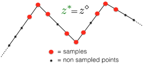
(a)

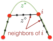
(b)

Figure 3: (a) Sampling corners and neighbors in 2D depth estimation guarantees exact recovery of the true profile. (b) Sampling only the corners does not guarantee, in general, that the solution of the $\ell_{1}$-minimization, namely ${z^{\star}}$, coincides with the true profile $z^{\diamond}$.

Proposition 7 implies that we can recover the original profile exactly, if we measure the neighborhood of each corner. An example that satisfies such condition is illustrated in Fig. 3(a). When we sample only the corners, however, Proposition 7 states that $C_{\text{er}}=1$; in principle in this case one might still hope to recover the profile $z^{\diamond}$, since the condition $C_{\text{er}}<1$ in Proposition 6 is only sufficient for exact recovery. But it turns out that in our problem one can find counterexamples with $C_{\text{er}}=1$ in which $\ell_{1}$-minimization fails to recover $z^{\diamond}$. A pictorial example is shown in Fig. 3(b), where we show an optimal solution ${z^{\star}}$ which differs from the true profile $z^{\diamond}$.

We derive a similar condition for 3D problems. The proof is given in Appendix C.

Proposition 8 (Exact Recovery of 3D depth profiles).

Let $Z^{\diamond}$ be a 3D depth profile with edge set ${\cal E}$. Assume noiseless measurements. If the sampling set ${\cal M}$ includes the edges and theirs (vertical and horizontal) neighbors (adjacent pixels), then $C_{\text{er}}=0$, and ($\text{L1}_{\Delta}$) recovers $\,\text{vec}{\left(Z^{\diamond}\right)}$ exactly.

In the experimental section, we show that these initial results already unleash interesting applications. For instance, in stereo vision problems, we could locate the position of the edges from the RGB images and recover the depth in a neighborhood of the edge pixels. Then, the complete depth profile can be recovered (at arbitrary resolution) via ($\text{L1}_{\Delta}$).

V-B Depth Reconstruction from Noiseless Samples

The exact recovery conditions of Proposition 7 and Proposition 8 are quite restrictive if we do not have prior knowledge of the position of the corners or edges. In this section we provide more powerful results that do not require sampling corners or edges. Empirically, we observe that when we do not sample all the edges, the optimization problems ($\text{L1}_{D}$) and ($\text{L1}_{\Delta}$) admit multiple solutions, i.e., multiple profiles $z$ attain the same optimal cost. The basic questions addressed in this section are: which profiles are in the solution set ${{\cal S}^{\star}}$ of problems ($\text{L1}_{D}$) and ($\text{L1}_{\Delta}$)? Is the ground truth profile $z^{\diamond}$ among these optimal solutions? How far can an optimal solution be from the ground truth profile $z^{\diamond}$? In order to answer these questions, in this section we derive optimality conditions for problems ($\text{L1}_{D}$) and ($\text{L1}_{\Delta}$), under the assumption that all measurements are noise-free.

V-B1 Algebraic Optimality Conditions (noiseless samples)

In this section, we derive a general algebraic condition for a 2D profile (resp. 3D) to be in the solution set of ($\text{L1}_{D}$) (resp. ($\text{L1}_{\Delta}$)). Section V-B2 and Section V-B3 translate this algebraic condition into a geometric constraint on the curvature of the profiles in the solution set.

Proposition 9 (2D Optimality).

Let $A$ be the sampling matrix and ${\cal M}$ be the sample set. Given a profile $z\in{{\mathbb{R}}^{n}}$ which is feasible for ($\text{L1}_{D}$), $z$ is a minimizer of ($\text{L1}_{D}$) if and only if there exists a vector $u$ such that

$$(D^{\mathsf{T}})_{\overline{{\cal M}}}\;u={\mathbf{0}}\;\text{ and }\;u_{\cal I}=\text{sign}(Dz)_{\cal I}\;\text{ and }\;\|u\|_{\infty}\leq 1$$ (14)

where ${\cal I}$ is the $D$-support of $z$ (i.e., the set of indices of the nonzero entries of $Dz$) and $\overline{{\cal M}}$ is the set of entries of $z$ that we do not sample (i.e., the complement of ${\cal M}$).

The proof of Proposition 9 is based on the subdifferential of the $\ell_{1}$-minimization problem and is provided in Appendix D. An analogous result holds in 3D.

Corollary 10 (3D optimality).

A given profile $Z$ is in the set of minimizers of ($\text{L1}_{\Delta}$) if and only if the conditions of Proposition 9 hold, replacing $D$ with $\Delta$ in eqs. (14).

We omit the proof of Corollary 10 since it follows the same line of the proof of Proposition 9.

V-B2 Analysis of 2D Reconstruction (noiseless samples)

In this section we derive necessary and sufficient geometric conditions for $z^{\diamond}$ to be in the solution set of ($\text{L1}_{D}$). Using these findings we obtain two practical results: (i) an upper bound on how far any solution ${z^{\star}}$ of ($\text{L1}_{D}$) can be from the ground truth profile $z^{\diamond}$; (ii) a general algorithm that recovers $z^{\diamond}$ even when the conditions of Proposition 7 fail (the algorithm is presented in Section VI-A).

To introduce our results, we need the following definition.

Definition 11 (2D Sign Consistency).

Let $s_{k}=\text{sign}(z_{k-1}-2z_{k}+z_{k+1})$ (sign of the curvature at $k$). A 2D depth profile $z$ is sign consistent if, for any two consecutive samples $i<j\in{\cal M}$, one of the two conditions holds:

1. no sign change: for any two integers $k,h$, with $i\leq k,h\leq j$, if $s_{k}\neq 0$ and $s_{h}\neq 0$, then $s_{k}=s_{h}$;

2. sign change only at the boundary: for any integer $k$, with $i<k<j$, $s_{k}=0$;

This technical definition has a clear geometric interpretation. In words, a profile $z$ is sign consistent, if its curvature does not change sign (i.e., it is either convex or concave) within each interval between consecutive samples. See Fig. 4 for examples of sign consistency, alongside with a counter-example.

(a)

(b)

Figure 4: Examples of sign-consistent (shown in black) and sign-inconsistent (shown in blue) 2D depth profile.

In the following we show that any optimal solutions for problem ($\text{L1}_{D}$) must be sign consistent. In order to simplify the analysis for Theorem 13 below, we assume that we pick pairs of consecutive samples (rather than individual, isolated samples). We formalize this notion as follows.

Definition 12 (Twin samples).

A twin sample is a pair of consecutive samples, i.e., $(i,i+1)$ with $i\in\{1,\ldots,n-1\}$.

Theorem 13 (2D Sign Consistency $\Leftrightarrow$ Optimality).

Let $z$ be a 2D profile which is feasible for problem ($\text{L1}_{D}$). Assume that the sample set includes only twin samples and we sample the “boundary” of the profile, i.e., $z_{1}$, and $z_{n}$. Then, $z$ is optimal for ($\text{L1}_{D}$) if and only if it is sign consistent.

The proof of Theorem 13 is given in Appendix E. This theorem provides a tight geometric condition for a profile to be optimal. More specifically, a profile is optimal for problem ($\text{L1}_{D}$) if it passes through the given set of samples (i.e., it satisfies the constraint in ($\text{L1}_{D}$)) and does not change curvature between consecutive samples. This result also provides insights into the conditions under which the ground truth profile will be among the minimizers of ($\text{L1}_{D}$), and how one can bound the depth estimation error, as stated in the following proposition.

Proposition 14 (2D Recovery Error - noiseless samples).

Let $z^{\diamond}$ be the ground truth profile generating noiseless measurements (4). Assume that we sample the boundary of $z^{\diamond}$ and the sample set includes a twin sample in each linear segment in $z^{\diamond}$. Then, $z^{\diamond}$ is in the set of minimizers of ($\text{L1}_{D}$). Moreover, denote with $\tilde{z}$ the naive solution obtained by connecting consecutive samples with a straight line (linear interpolation). Then, any optimal solution ${z^{\star}}$ lies between $z^{\diamond}$ and $\tilde{z}$, i.e., for any index $i\in\{1,\ldots,n\}$, it holds $\min(z^{\diamond}_{i},\tilde{z}_{i})\leq{z_{i}^{\star}}\leq\max(z^{\diamond}_{i},\tilde{z}_{i})$. Moreover, it holds

$$\|z^{\diamond}-{z^{\star}}\|_{\infty}\leq\max_{i\in{\cal M}}d_{i}\cos(\theta_{i})$$ (15)

where $d_{i}$ is the distance between the sample $i$ and the nearest corner in $z^{\diamond}$, while $\theta_{i}$ is the angle that the line connecting $i$ with the nearest corner forms with the vertical.

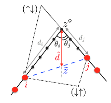
(a)

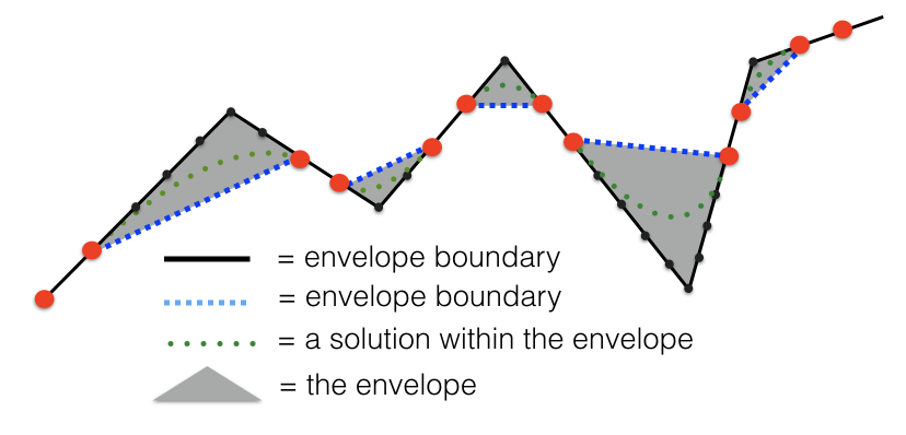
(b)

Figure 5: (a) Region between a pair of twin samples, with twin samples not including corners. (b) Given a set of noiseless twin samples, all possible optimal solutions in 2D are contained in the envelope shown in gray.

A visualization of the parameters $d_{i}$ and $\theta_{i}$ is given in Fig. 5(a). The proof of Proposition 14 is given in Appendix F.

Proposition 14 provides two important results. First, it states that any optimal solution ${z^{\star}}$ (e.g., the dotted green line in Fig. 2(b)) should lie between the ground truth depth $z^{\diamond}$ (solid black line) and the naive solution $\tilde{z}$ (dashed blue line). In other words, any arbitrary set of twin samples defines an envelope that contains all possible solutions. An example of such envelope is illustrated in Fig. 5(b). The width of this envelope bounds the maximum distance between any optimal solution and the ground truth, and hence such envelope provides a point-wise quantification of the reconstruction error. Second, Proposition 14 provides an upper bound on the overall reconstruction error in eq. (15). The inequality implies that the reconstruction error grows with the parameter $d_{i}$, the distance between our samples and the corners. In addition, the error also increases if the parameter $\theta_{i}$ is small, meaning that the ground truth profiles are “pointy” and there exist abrupt changes of slope between consecutive segments. An instance of such “pointy” behavior is the second corner from right in Fig. 5(b).

We will further show in Section VI that Proposition 14 has algorithmic implications. Based on Proposition 14, we design an algorithm that exactly recovers a 2D profile, even when the sample set does not contain all corners. Before moving to algorithmic aspects, let us consider the 3D case.

V-B3 Analysis of 3D Reconstruction (noiseless samples)

In this section we provide a sufficient geometric condition for a 3D profile to be in the solution set of ($\text{L1}_{\Delta}$). We start by introducing a specific sampling strategy (the analogous of the twin samples in 2D) to simplify the analysis.

Definition 15 (Grid samples and Patches).

Given a 3D profile $Z\in\mathbb{R}^{r\times c}$, a grid sample set includes pairs of consecutive rows and columns of $Z$, along with the boundaries (first and last two rows, first and last two columns). This sampling strategy divides the image in rectangular patches, i.e., sets of non-sampled pixels enclosed by row-samples and column-samples.

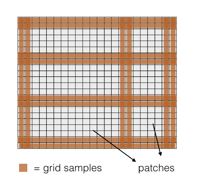
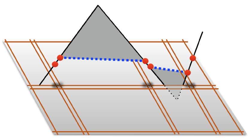
(a) (b)

Figure 6: (a) Illustration of a grid sample set, along with 6 non-sampled patches in white. (b) A cross section of the envelope in 3D.

Fig. 6(a) shows an example of grid samples and patches. If we have $K$ patches and we denote the set of non-sampled pixels in patch $i$ with $\overline{{\cal M}}_{i}$, then the union ${\cal M}\cup\{\overline{{\cal M}}_{i}\}_{i=1}^{K}$ includes all the pixels in the depth image. We can now extend the notion of sign consistency to the 3D case.

Definition 16 (3D Sign Consistency).

Let $Z\in\mathbb{R}^{r\times c}$ be a 3D depth profile. Let ${\cal M}$ be a grid sampling set and $\{\overline{{\cal M}}_{i}\}_{i=1}^{K}$ be the non-sampled patches. Let $Z_{[\overline{{\cal M}}_{i}]}$ be the restriction of $Z$ to its entries in $\overline{{\cal M}}_{i}$. Then, $Z$ is called 3D sign consistent if for all $i=\{1,\ldots,K\}$, the nonzero entries of $\text{sign}(\text{vec}(DZ_{[\overline{{\cal M}}_{i}]}))$ are all $+1$ or $-1$, and the nonzero entries of $\text{sign}(\text{vec}(Z_{[\overline{{\cal M}}_{i}]}D^{\mathsf{T}}))$ are all $+1$ or $-1$, where $D$ is the 2^nd-order difference operator (6) of suitable dimension.

Intuitively, 3D sign consistency indicates that the sign of the profile’s curvature does not change, either horizontally or vertically, within each non-sampled patch. We now present a sufficient condition for $Z^{\diamond}$ to be in the solution set of ($\text{L1}_{\Delta}$).

Theorem 17 (3D Sign Consistency $\Rightarrow$ Optimality).

Let $Z\in\mathbb{R}^{r\times c}$ be a 3D profile, feasible for problem ($\text{L1}_{\Delta}$). Assume the sample set ${\cal M}$ is a grid sample set. Then $Z$ is in the set of minimizers of ($\text{L1}_{\Delta}$) if it is 3D sign consistent.

The proof is given in Appendix G. Theorem 17 is weaker than Theorem 13, the 2D counterpart, since our definition of 3D sign consistency is only sufficient, but not necessary, for optimality. Nevertheless, it can be used to bound the depth recovery error as follows.

Proposition 18 (3D Recovery Error - noiseless samples).

Let $Z^{\diamond}\in\mathbb{R}^{r\times c}$ be the ground truth profile generating noiseless measurements (4). Let ${\cal M}$ be a grid sampling set and assume $Z^{\diamond}$ to be 3D sign consistent with respect to ${\cal M}$. Moreover, let $\underline{Z}\in\mathbb{R}^{r\times c}$ and $\bar{Z}\in\mathbb{R}^{r\times c}$ be the point-wise lower and upper bound of the row-wise envelope, built as in Fig. 5(b) by considering each row of the 3D depth profile as a 2D profile. Then, $Z^{\diamond}$ is an optimal solution of ($\text{L1}_{\Delta}$), and any other optimal solution ${Z^{\star}}$ of ($\text{L1}_{\Delta}$) satisfies:

$$|Z^{\diamond}_{i,j}-Z^{\star}_{i,j}|\leq\max(|\underline{Z}_{i,j}-{Z^{\star}}_{i,j}|,|\bar{Z}_{i,j}-{Z^{\star}}_{i,j}|)$$ (16)

Roughly speaking, if our grid sampling is “fine” enough to capture all changes in the sign of the curvature of $Z^{\diamond}$, then $Z^{\diamond}$ is among the solutions of ($\text{L1}_{\Delta}$). Despite the similarity to Proposition 14, the result in Proposition 18 is weaker. More specifically, Proposition 18 is based on the fact that we can compute an envelope only for the ground truth profile (but not for all the optimal solutions, as in Proposition 14). Moreover, the estimation error bound in eq. (16) can be only computed a posteriori, i.e., after obtaining an optimal solution ${Z^{\star}}$. Nevertheless, the result can be readily used in practical applications, in which one wants to bound the depth estimation error. An example of the row-wise envelope is given in Fig. 6(b).

V-C Depth Reconstruction from Noisy Samples

In this section we analyze the depth reconstruction quality for the case where the measurements (4) are noisy. In other words, we now focus on problems ($\text{L1}_{D}^{\varepsilon}$) and ($\text{L1}_{\Delta}^{\varepsilon}$).

V-C1 Algebraic Optimality Conditions (noisy samples)

In this section, we derive a general algebraic condition for a 2D profile (resp. 3D) to be in the solution set of ($\text{L1}_{D}^{\varepsilon}$) (resp. ($\text{L1}_{\Delta}^{\varepsilon}$)). This condition generalizes the optimality condition of Section V-B1 to the noisy case. In Section V-C2 and Section V-C3, we apply this algebraic condition to bound the depth reconstruction error.

Proposition 19 (2D robust optimality).

Let $A$ be the sampling matrix, ${\cal M}$ be the sample set and $y$ be the noisy measurements as in (4), with $\|\eta\|_{\infty}\leq\varepsilon$ and $\varepsilon>0$. Given a profile $z$ which is feasible for ($\text{L1}_{D}^{\varepsilon}$), define the active set ${\cal A}\subset{\cal M}$ as follows

$${\cal A}=\{i\,\in{\cal M}:|y_{i}-z_{i}|=\varepsilon\}.$$ (17)

We also define its two subsets

$${\cal A}_{\uparrow} =\{i\,\in{\cal M}:y_{i}-z_{i}=\varepsilon\},$$

$${\cal A}_{\downarrow} =\{i\,\in{\cal M}:y_{i}-z_{i}=-\varepsilon\}.$$ (18)

Also denote $\bar{{\cal A}}={\cal M}\setminus{\cal A}$. Then $z$ is a minimizer of ($\text{L1}_{D}^{\varepsilon}$) if and only if there exists a vector $u$ such that

$$(D^{\mathsf{T}})_{\overline{{\cal M}}\cup\bar{{\cal A}}}\;u\!=\!{\mathbf{0}}\;\text{ and }\;u_{\cal I}\!=\!\text{sign}(Dz)_{\cal I}\;\text{ and }\;\|u\|_{\infty}\leq 1$$ (19)

$$(D^{\mathsf{T}})_{\cal A}{}_{\uparrow}\;u\geq{\mathbf{0}}\;\text{ and }\;(D^{\mathsf{T}})_{\cal A}{}_{\downarrow}\;u\leq{\mathbf{0}}$$ (20)

where ${\cal I}$ is the $D$-support of $z$, and $\overline{{\cal M}}$ is the set of un-sampled entries in $z$ (i.e., the complement of ${\cal M}$).

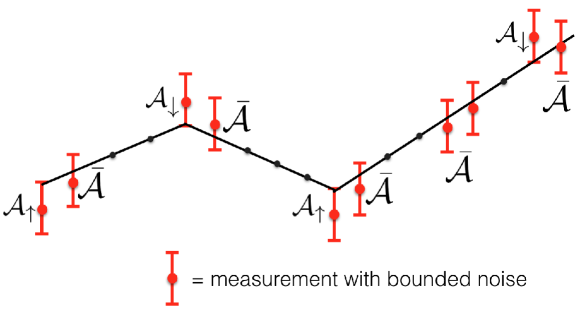
Figure 7: A illustration of the active set ${\cal A}$ of samples in Proposition 19. The three corners, as well as the second sample from the right, are all within the active set. A measurement $y_{i}$ is active if the reconstructed profile z hits the boundary of $y_{i}$’s associated error bound.

The proof is given in Appendix I. A visual illustration of the active set is given in Fig. 7. We will provide some geometric insights on the algebraic conditions in Proposition 19 in the next two sections. Before moving on, we re-ensure that the robust optimality conditions straightforwardly extends to the 3D case.

Corollary 20 (3D robust optimality).

A given profile $Z$ is in the set of minimizers of ($\text{L1}_{\Delta}^{\varepsilon}$) if and only if the conditions of Proposition 19 hold, replacing $\Delta$ with $D$ in eqs. (19)-(20).

We skip the proof of Corollary 20 since it proceeds along the same line of the proof of Proposition 19.

V-C2 Analysis of 2D Reconstruction (noisy samples)

In this section we consider the 2D case and provide a geometric interpretation of the algebraic conditions in Proposition 19. The geometric interpretation follows from a basic observation, which enables us to relate the noisy case with our noiseless analysis of Section V-B2. The observation is that if a profile satisfies the robust optimality conditions (19)-(20) then it also satisfies the noiseless optimality condition (14), hence being sign consistent, as per Theorem 13.

Theorem 21 (Robust optimality $\Rightarrow$ 2D Sign Consistent).

Let ${z^{\star}}$ be a 2D profile which is optimal for problem ($\text{L1}_{D}^{\varepsilon}$), and assume that the sample set includes only twin samples and we sample the “boundary” of the profile, i.e., $z_{1}$, and $z_{n}$. Then, ${z^{\star}}$ is 2D sign consistent.

We present a brief proof for Theorem 21 below.

Proof.

Note that $(D^{\mathsf{T}})_{\overline{{\cal M}}\cup\overline{{\cal A}}}\;u\!=\!{\mathbf{0}}\;\;\Rightarrow\;\;(D^{\mathsf{T}})_{\overline{{\cal M}}}\;u\!=\!{\mathbf{0}}$. In other words, condition (19) implies condition (14), which in turn is equivalent to sign consistency as per Theorem 13. Therefore, we come to the conclusion that any optimal solution of ($\text{L1}_{D}^{\varepsilon}$) must be sign consistent. ∎

Theorem 21 will help establish error bounds on the depth reconstruction. Before presenting these bounds, we formally define the 2D sign consistent $\epsilon$-envelope.

Definition 22 (2D Sign Consistent $\epsilon$-envelope).

Assume that the sample set includes only twin samples and we sample the “boundary” of the profile, i.e., $z_{1}$, and $z_{n}$. Moreover, for each pair of consecutive twin samples $i,i+1$ and $j,j+1$, define the following line segments for $k\in(i+1,j)$:

1. $\frac{z_{k}-(y_{i}-\varepsilon)}{x_{k}-x_{i}}=\frac{(y_{i+1}+\varepsilon)-(y_{i}-\varepsilon)}{x_{i+1}-x_{i}}$

2. $\frac{z_{k}-(y_{i}+\varepsilon)}{x_{k}-x_{i}}=\frac{(y_{i+1}-\varepsilon)-(y_{i}-\varepsilon)}{x_{i+1}-x_{i}}$

3. $\frac{z_{k}-(y_{j+1}-\varepsilon)}{x_{k}-x_{j+1}}=\frac{(y_{j}+\varepsilon)-(y_{j+1}-\varepsilon)}{x_{j}-x_{j+1}}$

4. $\frac{z_{k}-(y_{j+1}+\varepsilon)}{x_{k}-x_{j+1}}=\frac{(y_{j}-\varepsilon)-(y_{j+1}+\varepsilon)}{x_{j}-x_{j+1}}$

5. $\frac{z_{k}-(y_{i+1}+\varepsilon)}{x_{k}-x_{i+1}}=\frac{(y_{j}+\varepsilon)-(y_{i+1}+\varepsilon)}{x_{j}-x_{i+1}}$

6. $\frac{z_{k}-(y_{i+1}-\varepsilon)}{x_{k}-x_{i+1}}=\frac{(y_{j}-\varepsilon)-(y_{j+1}-\varepsilon)}{x_{j}-x_{j+1}}$

Further define the following profiles:

$$\bar{z}:=\left\{\begin{array}[]{ll}\mathrm{\max\{(1),(3),(5)\}},&\ \ \ \text{if (1) and (3) intersect}\\ \mathrm{(5)},&\ \ \ \text{otherwise}\end{array}\right.$$

and

$$\underline{z}:=\left\{\begin{array}[]{ll}\mathrm{\max\{(2),(4),(6)\}},&\ \ \ \text{if (2) and (4) intersect}\\ \mathrm{(6)},&\ \ \ \text{otherwise}\end{array}\right.$$

where $\mathrm{\max\{(1),(3),(5)\}}$ denotes the point-wise maximum among the segments in eqs. (1), (3), and (5). We define the 2D sign consistent $\epsilon$-envelope as the region enclosed between the upper bound $\bar{z}\in{{\mathbb{R}}^{n}}$ and the lower bound $\underline{z}\in{{\mathbb{R}}^{n}}$.

A pictorial representation of the line segments (1)-(6) in Definition 22 is given in Fig. 8(a)-(b). Fig. 8(a) shows an example where line segment (1) intersects with (3) and line segment (2) intersects with (4). In Fig. 8(b), these line segments do no intersect. An example of the resulting 2D sign consistent $\epsilon$-envelope is illustrated in Fig. 8(c).

Our interest towards the 2D sign consistent $\epsilon$-envelope is motivated by the following proposition.

Proposition 23 (2D Sign Consistent $\epsilon$-envelope).

Under the conditions of Definition 22, any 2D sign-consistent profile, belongs to the 2D sign consistent $\epsilon$-envelope.

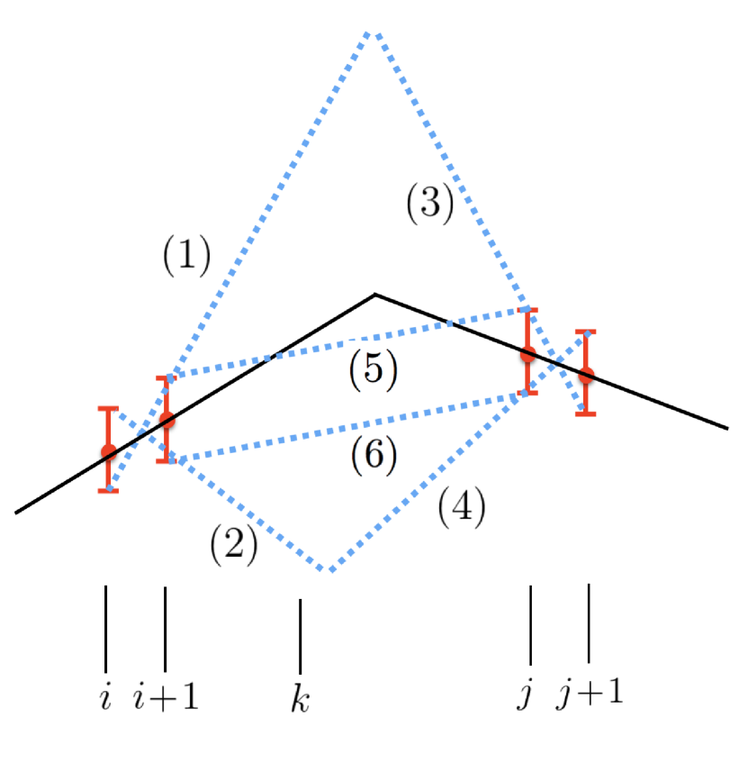
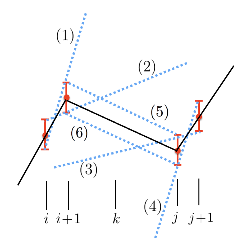
(a) (b)

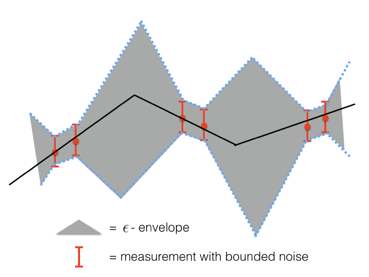
(c)

Figure 8: (a) Illustration of the line segments (1)-(6) in Definition 22 with intersection. (b) Line segments (1)-(6) without intersection. (c) An example of 2D sign consistent $\epsilon$-envelope.

The proof of Proposition 23 is given in Appendix J.

Next we introduce a proposition that characterizes the depth reconstruction error bounds of an optimal solution.

Proposition 24 (2D Recovery Error - noisy samples).

Let $z^{\diamond}\in{{\mathbb{R}}^{n}}$ be the ground truth generating noisy measurements (4). Assume that we sample the boundary of $z^{\diamond}$ and the sample set includes a twin sample in each linear segment in $z^{\diamond}$. Then, $z^{\diamond}$ belongs to the 2D sign consistent $\epsilon$-envelope, and any optimal solution ${z^{\star}}$ of ($\text{L1}_{D}^{\varepsilon}$) also lies in the $\epsilon$-envelope. Moreover, denoting with $\underline{z}\in{{\mathbb{R}}^{n}}$ and $\bar{z}\in{{\mathbb{R}}^{n}}$, the point-wise lower and upper bound of the $\epsilon$-envelope (Definition 22), and considering any consecutive pairs of twin samples $i,i+1$ and $j,j+1$, for all $k\in(i+1,j)$, it holds:

$$|z^{\diamond}_{k}-{z_{k}^{\star}}|\leq\bar{z}_{k}-\underline{z}_{k}.$$

The proof of Proposition 24 is given in Appendix K.

V-C3 Analysis of 3D Reconstruction (noisy samples)

In this section we characterize the error bounds of an optimal solution ${Z^{\star}}$ of ($\text{L1}_{\Delta}^{\varepsilon}$) in the noisy case. The result is similar to its noiseless counterpart in Proposition 18.

Proposition 25 (3D Recovery Error - noisy samples).

Let $Z^{\diamond}\in\mathbb{R}^{r\times c}$ be the ground truth generating noisy measurements (4). Let ${\cal M}$ be a grid sample set and assume $Z^{\diamond}$ to be 3D sign consistent with respect to ${\cal M}$. Moreover, let $\underline{Z}\in\mathbb{R}^{r\times c}$ and $\bar{Z}\in\mathbb{R}^{r\times c}$ be the point-wise lower and upper bound of the row-wise 2D sign consistent $\epsilon$-envelope, built as in Fig. 8(b) by considering each row of the 3D depth profile as a 2D profile. Then, given any optimal solution ${Z^{\star}}$ of ($\text{L1}_{\Delta}^{\varepsilon}$), it holds that

$$|Z^{\diamond}_{i,j}-Z^{\star}_{i,j}|\leq\max(|\underline{Z}_{i,j}-{Z^{\star}}_{i,j}|,|\bar{Z}_{i,j}-{Z^{\star}}_{i,j}|)$$ (21)

The proof for Proposition 25 follows the same line as the proof of Proposition 18, and we omit the proof for brevity.

VI Algorithms and Fast Solvers

The formulations discussed so far, namely ($\text{L1}_{D}$), ($\text{L1}_{D}^{\varepsilon}$), ($\text{L1}_{\Delta}$), ($\text{L1}_{\Delta}^{\varepsilon}$), directly translate into algorithms: each optimization problem can be solved using standard convex programming routines and returns an optimal depth profile.

This section describes two algorithmic variants that further enhance the quality of the depth reconstruction (Section VI-A), and then presents a fast solver for the resulting $\ell_{1}$-minimization problems (Section VI-B).

input : Measurements $y$, and sample set ${\cal M}$, including boundary and twin samples

output :  Original profile $z^{\diamond}$

/* solve $\ell_{1}$-minimization */

1 create matrices $A$ (Definition 3) and $D$ (eq. (6)) ;

2 solve $(f^{\star},{z^{\star}})=\min_{z}\;\|Dz\|_{1}\quad\text{ subject to }Az=y$ ;

/* populate a vector of signs $s\in\{-1,0,+1\}^{n}$ */

3 for consecutive twin samples $(i-1,i)$, ($j,j+1$) do

4       foreach $k\in\{i+1,\ldots,j-1\}$ do

5             set $s_{k}=\text{sign}((z^{\star}_{j+1}-z^{\star}_{j})-(z^{\star}_{i}-z^{\star}_{i-1}))$

6      

/* recover $z^{\diamond}$ within the solution set */

7 $z^{\diamond}=\mathrm{argmin}_{z}\;s^{\mathsf{T}}z\quad\text{ subject to }Az=y\text{ and }\|Dz\|_{1}\leq f^{\star}$ ;

return $z^{\diamond}$.

Algorithm 1 Exact recovery of 2D depth profiles.

VI-A Enhanced Recovery in 2D and 3D

In this section we describe other algorithmic variants for the 2D and 3D case. Section VI-A1 proposes a first algorithm that solves 2D problems and is inspired by Proposition 14. Section VI-A2 discusses variants of ($\text{L1}_{\Delta}$) for 3D problems.

VI-A1 Enhanced Recovery in 2D problems

Proposition 14 dictates that any optimal solution of ($\text{L1}_{D}$) lies between the naive interpolation solution and the ground truth profile $z^{\diamond}$ (recall Fig. 2(b)). Algorithm 1 is based on a simple idea: on the one hand, if the true profile is concave between two consecutive samples (cf. with the first corner in Fig. 2(b)), then we should look for an optimal profile having depth “as large as possible” in that particular interval (while still being within the optimal set of ($\text{L1}_{D}$)); on the other hand, if the shape is convex (second corner in Fig. 2(b)) we should look for an optimal profile with depth as “as small as possible”, since this is the closest to $z^{\diamond}$.

Algorithm 1 first solves problem ($\text{L1}_{D}$) and computes an optimal solution ${z^{\star}}$ and the corresponding optimal cost $f^{\star}$ (lines 1-1). Let us skip lines 1-1 for the moment and take a look at line 1: the constraints in this optimization problem include the same constraint of line 1 ($Az=y$), plus an additional constraint in line 1 ($\|Dz\|_{1}\leq f^{\star}$) that restricts $z$ to stay within the optimal solution set of ($\text{L1}_{D}$). Therefore, it only remains to design a new objective function that “encourages” a solution that is close to $z^{\diamond}$ while still being within this optimal set. To this end, we use a simple linear objective $s^{\mathsf{T}}z$, where $s\in\{0,\pm 1\}^{n}$ is a vector of coefficients, such that the objective function penalizes large entries in the profile $z$ if $s_{k}=+1$, and rewards large entries when $s_{k}=-1$. More specifically, the procedure for choosing a proper coefficient $s_{k}$ is as follows. For any consecutive pairs of twin samples $(i-1,i)$ and ($j,j+1$), the algorithm looks at the slope difference between the second pair (i.e., $z^{\star}_{j+1}-z^{\star}_{j}$) and the first pair ($z^{\star}_{i}-z^{\star}_{i-1}$). If this difference is negative, then the function ${z^{\star}}$ is expected to be concave between the samples. In this case the sign $s_{k}$ for any point $k$ between the samples is set to $-1$. If the difference is positive, then the signs are set to $+1$. Otherwise the signs will be 0. We prove the following result.

Corollary 26 (Exact Recovery of 2D profiles by Algorithm 1).

Under the assumptions of Proposition 14, Algorithm 1 recovers the 2D depth profile $z^{\diamond}$ exactly.

The proof is in Appendix L. Although Algorithm 1 is designed for noiseless samples, in the experiments in Section VII-A we also test a noisy variant by substituting the constraints in lines 1 and 1 with $\|Az-y\|_{\infty}\leq\varepsilon$.

VI-A2 Enhanced Recovery in 3D problems

In the formulations ($\text{L1}_{\Delta}$) and ($\text{L1}_{\Delta}^{\varepsilon}$) we used the matrix $\Delta$ to encourage “flatness”, or in other words, regularity of the depth profiles. In this section we discuss alternative objective functions which we evaluate experimentally in Section VII. These objectives simply adopt different definitions for the matrix $\Delta$ in ($\text{L1}_{\Delta}$) and ($\text{L1}_{\Delta}^{\varepsilon}$). For clarify, we denote the formulation introduced earlier in this paper (using the matrix $\Delta$ defined in (12)) as the “L1” formulation (also recalled below), and we introduce two new formulations, denoted as “L1diag” and “L1cart”, which use different objectives.

L1 formulation: Although we already discussed the structure of the matrix $\Delta$ in Section IV-C, here we adopt a slightly different perspective that will make the presentation of the variants L1diag and L1cart clearer. In particular, rather than taking a matrix view as done in Section IV-C, we interpret the action of the matrices $D_{V}$ and $D_{H}$ in eq. (10) as the application of a kernel (or convolution filter) to the 3D depth profile $Z$. In particular, we note that:

$$D_{V}Z=Z*K_{xx}\qquad(ZD_{H}^{\mathsf{T}})^{\mathsf{T}}=Z*K_{yy}$$ (22)

where “$*$” denotes the action of a discrete convolution filter and the kernels $K_{xx}$ and $K_{yy}$ are defined as

$$K_{xx}=\begin{bmatrix}0&0&0\\ 1&-2&1\\ 0&0&0\end{bmatrix},\quad K_{yy}=\begin{bmatrix}0&1&0\\ 0&-2&0\\ 0&1&0\end{bmatrix}.$$

Intuitively, $K_{xx}$ and $K_{yy}$ applied at a pixel return the 2^nd-order differences along the horizontal and vertical directions at that pixel, respectively. The L1 objective, presented in Section IV-C, can be then written as:

$$f_{\text{{\tt L1}}}(Z)\doteq\|\,\text{vec}{\left(Z*K_{xx}\right)}\|_{1}+\|\,\text{vec}{\left(Z*K_{yy}\right)}\|_{1}.$$

L1diag formulation: While L1 only penalizes, for each pixel, variations along the horizontal and vertical direction, the objective of the L1diag formulation includes an additional 2^nd-order derivative, which penalizes changes along the diagonal direction. This additional term can be written as $\|\,\text{vec}{\left(Z*K_{xy}\right)}\|_{1}$, where the kernel $K_{xy}$ is:

$$\begin{split}K_{xy}&=\frac{1}{4}*\begin{bmatrix}-1&0&1\\ 0&0&0\\ 1&0&-1\end{bmatrix}.\end{split}$$

Therefore, the objective in the L1diag formulation is

$$f_{\text{{\tt L1diag}}}(Z)\doteq f_{\text{{\tt L1}}}(Z)+\|\,\text{vec}{\left(Z*K_{xy}\right)}\|_{1}.$$

L1cart formulation: When introducing the L1 formulation in Section IV, we assumed that we reconstruct the depth at uniformly-spaced point, i.e., the $(x,v)$ coordinates of each point belong to a uniform grid; in other words, looking at the notion of curvature in (5), we assumed $x_{i+1}-x_{i}=x_{i}-x_{i-1}=1$ (also $v_{i+1}-v_{i}=v_{i}-v_{i-1}=1$ in the 3D case). While this comes without loss of generality, since the full profile is unknown and we can reconstruct it at arbitrary resolution, we note that typical sensors, even in 2D, do not produce measurements with uniform spacing, see Fig. 9.

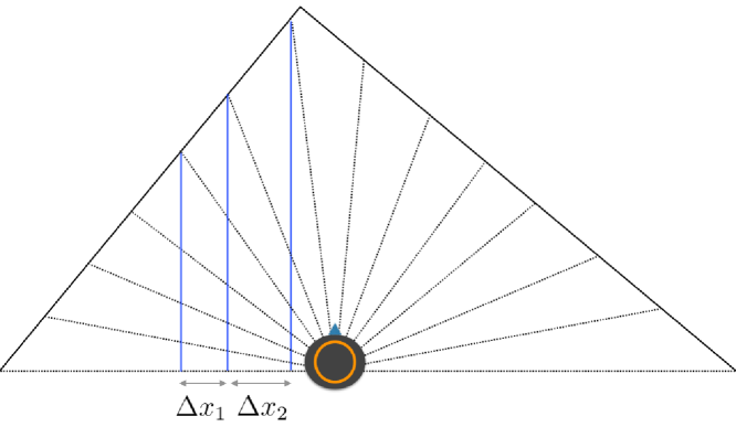
Figure 9: A toy example illustrating that while a 2D lidar produces measurements at fixed angular resolution, the resulting Cartesian coordinates are not equally spaced, i.e., $\Delta x_{1}\not=\Delta x_{2}$. This occurs in both lidars and perspective cameras, hence motivating the introduction of the L1cart formulation.

For this reason, in this section we generalize the L1 objective to account for irregularly-spaced points. If we denote with $x_{i,j}$ and $v_{i,j}$ the horizontal and vertical coordinates of the 3D point observed at pixel $(i,j)$, a general expression for the horizontal and vertical 2^nd-order differences is:

$$Z*K_{xx}^{\text{{\tt L1}-cart}}\qquad\qquad Z*K_{yy}^{\text{{\tt L1}-cart}}$$ (23)

where the convolution kernels at pixel $(i,j)$ are defined as:

$$\begin{array}[]{ll}K_{xx}^{\text{cart}}(i,j)=\\ \begin{bmatrix}0&0&0\\ \frac{1}{x_{i,j}-x_{i-1,j}}&-(\frac{1}{x_{i,j}-x_{i-1,j}}+\frac{1}{x_{i+1,j}-x_{i,j}})&\frac{1}{x_{i+1,j}-x_{i,j}}\\ 0&0&0\end{bmatrix},\\ K_{yy}^{\text{cart}}(i,j)=\begin{bmatrix}0&\frac{1}{v_{i,j}-v_{i,j-1}}&0\\ 0&\frac{1}{v_{i,j}-v_{i,j-1}}-\frac{1}{v_{i,j+1}-v_{i,j}}&0\\ 0&\frac{1}{v_{i,j+1}-v_{i,j}}&0\end{bmatrix}\end{array}$$ (24)

The kernels $K_{xx}^{\text{cart}}(i,j)$ and $K_{yy}^{\text{cart}}(i,j)$ simplify to $K_{xx}$ and $K_{yy}$ when the points are uniformly spaced, and can be used to define a new objective function:

$$f_{\text{{\tt L1cart}}}(Z)\doteq\|\,\text{vec}{\left(Z*K_{xx}^{\text{{\tt L1}-cart}}\right)}\|_{1}+\|\,\text{vec}{\left(Z*K_{yy}^{\text{{\tt L1}-cart}}\right)}\|_{1}.$$

L1cart may be used to query the depth at arbitrary points and in this sense it is more general than L1. On the downside, we notice that extra care should be taken to ensure that the denominators in the entries of the kernels $K_{xx}^{\text{cart}}(i,j)$ and $K_{yy}^{\text{cart}}(i,j)$ do not vanish, and small denominators (close to zero) may introduce numerical errors. For this reason, in our tests, we add a small positive constant $\delta$ to all denominators.

VI-B Fast Solvers

All the formulations presented in this paper, including the algorithmic variants proposed in Section VI-A, rely on solving the optimization problems ($\text{L1}_{D}$), ($\text{L1}_{\Delta}$), ($\text{L1}_{\Delta}^{\varepsilon}$), and ($\text{L1}_{D}^{\varepsilon}$) efficiently. Despite the convexity of these problems, off-the-shelf solvers based on interior point methods tend to be slow and do not scale to very large problems. Recalling that in the 3D case, the number of unknown variables in our problems is equal to the number of non-sampled pixels in the depth map, these optimization problems can easily involve more than $10^{5}$ variables. Indeed, in the experiments in Section VII-B3 we show that off-the-self solvers such as cvx/MOSEK [69, 70] are quite slow and practically unusable for 3D profiles larger than $100\times 100$ pixels.

For these reasons, in this section we discuss a more efficient first-order method to solve these minimization problems. This solver is a variant of NESTA, an algorithm for fast $\ell_{1}$ minimization recently developed by [18] and based on Nesterov’s method for nonsmooth optimization [71, 72]. We tailor NESTA to our specific optimization problems with $\ell_{\infty}$-norm constraints, instead of the original $\ell_{2}$ norm used in [18]. In this section we focus on the 2D problem ($\text{L1}_{D}^{\varepsilon}$), since the algorithm is identical in the 3D case (with the only exception that the matrix $\Delta$ is used in place of $D$).

input : Measurements $y$, sampling matrix $A$, noise level $\varepsilon$, initial guess $z^{(0)}$, desired final smoothing parameter value $\mu_{f}$, maximum Nesterov’s iterations $K$, continuation steps $T$, stopping criterion $\tau$

output :  Approximate solution $z^{(K)}$ for ($\text{L1}_{D}^{\varepsilon}$)

/* initialize parameters */

1 initialize $\mu_{0}=\|D^{\mathsf{T}}y\|_{\infty}$ ;

2 compute $\gamma=(\mu_{f}-\mu_{0})^{1/T}$ ;

/* outer iterations with decreasing $\mu$ */

3 for  $t=1:T$ do

4       set $\mu=\mu_{t-1}$ ;

       /* Nesterov’s accelerated gradient */

5       for $k=0:K-1$ do

6             compute $\nabla f_{\mu}(z^{(k)})$ ;

7             set $\alpha_{k}=\frac{k+1}{2}$ and $\tau_{k}=\frac{2}{k+3}$ ;

             /* solve: */

8             $\!\!\bar{q}=\mathrm{argmin}_{z}\;\frac{L_{\mu}}{2}\|z-z^{(k)}\|_{2}^{2}+{\langle}\nabla f_{\mu}(z^{(k)}),z-z^{(k)}{\rangle}$

9            $\hskip 21.33955pt\text{ subject to }\|Az-y\|_{\infty}\leq\varepsilon$ ;

10             $\!\!\bar{w}\!\!=\!\mathrm{argmin}_{z}\;\frac{L_{\mu}}{2}\|z\!-\!z^{(0)}\|_{2}^{2}+\!\displaystyle\sum_{i=0}^{k}\alpha_{i}{\langle}\nabla f_{\mu}(z^{(i)}),z\!-\!z^{(k)}{\rangle}\!\!$ $\hskip 17.64056pt\text{ subject to }\|Az-y\|_{\infty}\leq\varepsilon$ ;

             /* update $z$ */

11             $z^{(k+1)}=\tau_{k}\bar{w}+(1-\tau_{k})\bar{q}$ ;

             /* stopping criterion */

12             if $\|z^{(k+1)}-z^{(k)}\|_{\infty}<\tau$  then

13                   $z^{(K)}=z^{(k+1)}$;  break loop

14            

      /* decrease the value of $\mu$ */

15       set $\mu_{t}=\gamma\mu_{t-1}$ ;

16       set $z^{(0)}=z^{(K)}$ ;

17      

return $z^{(K)}$.

Algorithm 2 NESTA for solving ($\text{L1}_{D}^{\varepsilon}$)

In this section, we provide an overview of NESTA, adapted to problem ($\text{L1}_{D}^{\varepsilon}$), while we leave technical details to Appendix M. NESTA solves convex optimization problems with nonsmooth objectives, in the general form:

$$\min_{z}\;f(z)\quad\text{ subject to }z\in{\cal Q}$$ (25)

where $f(z)$ is a nonsmooth convex function and ${\cal Q}$ is a convex set. The basic idea in NESTA is to replace the original objective $f(z)$ with a smooth approximation $f_{\mu}(z)$

$$\min_{z}\;f_{\mu}(z)\quad\text{ subject to }z\in{\cal Q}$$ (26)

where $\mu$ is a parameter controlling the smoothness of $f_{\mu}(z)$ and such that when $\mu$ goes to zero, $f_{\mu}(z)$ approaches $f(z)$.

In our problem ($\text{L1}_{D}^{\varepsilon}$), we have $f(z)=\|Dz\|_{1}$ and ${\cal Q}=\{z:\|Az-y\|_{\infty}\leq\varepsilon\}$. Following [71], we first notice that our nonsmooth objective can be written as:

$$f(z)\doteq\|Dz\|_{1}=\max_{u:\|u\|_{\infty}\leq 1}{\langle}u,Dz{\rangle}.$$ (27)

Then a convenient choice for $f_{\mu}(z)$ is

$$f_{\mu}(z)=\max_{u:\|u\|_{\infty}\leq 1}{\langle}u,Dz{\rangle}-\mu\frac{\|u\|_{2}^{2}}{2}.$$ (28)

The function $f_{\mu}(z)$ is differentiable, see [71], and its gradient is Lipschitz with constant $L_{\mu}$ (Appendix M provides an explicit expression for the constant $L_{\mu}$). It can be readily noticed from eq. (28) that when $\mu$ goes to zero, $f_{\mu}(z)$ approaches our objective $f(z)$.

NESTA adopts a continuation approach, in that it solves a sequence of optimization problems with decreasing values of $\mu$, such that the result of the last optimization problem approximates closely the solution of $f(z)$. The advantage in doing so is that, instead of minimizing directly $f(z)$ with nonsmooth optimization techniques which are generally slow, at each iteration NESTA applies Nesterov’s accelerated gradient method to the smooth function $f_{\mu}(z)$, ensuring an optimal convergence rate of ${\cal O}(1/K^{2})$ in the number of gradient iterations $K$.

The pseudo-code of NESTA, tailored to ($\text{L1}_{D}^{\varepsilon}$), is given in Algorithm 2. The outer iterations in line 2 iterate for decreasing values of $\mu$, starting at an initial value $\mu_{0}$ (computed in line 2) till a user-specified final value $\mu_{f}$. The user also specifies the numbers of outer iterations $T$, such that at each iteration the value of $\mu$ is decreased by an amount $\gamma<1$, computed in line 2; the value of $\mu$ is decreased after each outer iteration, as shown in line 2. The choice of $\mu_{f}$ implies a trade-off between the speed of convergence (the convergence rate of solving (26) is proportional to the $\mu$ used in each iteration) and the accuracy of the smoothed approximation $f_{\mu}$, which consequently determines the NESTA’s overall accuracy. According to experiments in [18], decreasing $\mu_{f}$ by a factor of $10$ gives about $1$ additional digit of accuracy on the optimal value.

NESTA uses a warm start mechanism, such that the solution $z^{(K)}$ for a given $\mu$ is used as initial guess at the next iteration, as shown in line 2. Choosing a good initial guess for the first iteration (input $z^{(0)}$ in Algorithm 2) may also contribute to speed-up the solver. In our tests we used the naive solution (linear interpolation) as initial guess for NESTA.

For a given value of $\mu$, lines 2-2 describe Nesterov’s accelerated gradient method applied to the smooth problem with objective $f_{\mu}$. The accelerated gradient method involves $K$ inner iterations (line 2) and terminates if the change in the depth estimate is small (stopping condition in lines 2-2). Nesterov’s method updates the depth estimate $z^{(k+1)}$ (line 2) using a linear combination of intermediate variables $\bar{q}$ (line 2) and $\bar{w}$ (line 2). We refer the reader to [71] for more details. We provide closed-form expressions for the gradient $\nabla f_{\mu}(z)$ and for the vectors $\bar{q}$ and $\bar{w}$ (lines 2-2) in Appendix M.

Note that when $\varepsilon=0$, Algorithm 2 solves the noiseless problem ($\text{L1}_{D}$). This only affects the closed-form solutions for $\bar{q}$ and $\bar{w}$, but does not alter the overall structure of the algorithm. Similarly, Algorithm 2 can be used to solve problems ($\text{L1}_{\Delta}$) and ($\text{L1}_{\Delta}^{\varepsilon}$), after replacing the matrix $D$ with $\Delta$ in the definition of $f(z)$. As discussed earlier, the choice of a nonzero $\mu_{f}$ in NESTA will result in an approximate solution to the optimal solution of ($\text{L1}_{D}^{\varepsilon}$). Consequently, NESTA may produce slightly less accurate solutions, while being much faster than cvx. Our experimental results show that the accuracy loss is negligible if the parameter $\mu_{f}$ is chosen appropriately, see Section VII-B3.

VII Experiments

This section validates our theoretical derivations with experiments on synthetic, simulated, and real data. Empirical evidence shows that our recovery techniques perform very well in practice, in both 2D and 3D environments. Our algorithm is also more robust to noise than a naive linear interpolation, and outperforms previous work in both reconstruction accuracy and computational speed. We discuss a number of applications, including 2D mapping (Section VII-A), 3D depth reconstruction from sparse measurements (Section VII-C-VII-D), data compression applied to bandwidth-limited robot-server communication (Section VII-E), and super-resolution depth imaging (Section VII-F). For the 3D case, we also provide a Monte Carlo analysis comparing the different solvers and choices of the objective functions (Section VII-B).

In the following tests, we evaluate the accuracy of the reconstruction by the average pixel-wise depth error, i.e., $\frac{1}{n}\|{z^{\star}}-z^{\diamond}\|_{1}$, where $z^{\diamond}$ is the ground truth and ${z^{\star}}$ is the reconstruction, unless otherwise specified.

VII-A 2D Sparse Reconstruction and Mapping

In this section, we apply our algorithm to reconstruct 2D depth profiles (e.g., the data returned by a 2D laser scanner). We provide both a statistical analysis on randomly generated synthetic profiles (Sections VII-A1-VII-A2), and a realistic example of application to 2D mapping (Section VII-A3).

VII-A1 Typical Examples of 2D Reconstruction

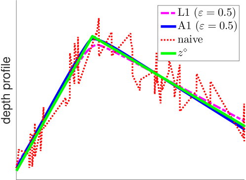
Figure 10: An example of synthetic 2D profile and typical behavior of the compared techniques, naive, L1, and A1, for noise level $\varepsilon=0.05\text{m}$.

We create a synthetic dataset that contains random piecewise linear depth profiles of size $n\!=\!2000$, with given number of corners. Since the number of variables is small, we use cvx/MOSEK [69, 70] as solver in all 2D experiments. When possible, we compare three different reconstruction algorithms: (i) the linear interpolation produced by Matlab’s command intep1, denoted as naive, (ii) the estimate from ($\text{L1}_{D}$) (noiseless case) or ($\text{L1}_{D}^{\varepsilon}$) (noisy case), denoted as L1, and (iii) the estimate produced by Algorithm 1, denoted as A1.

An example of synthetic 2D profile (with only one corner) is shown in Fig. 10. The green line is the ground truth profile, while the others are reconstructed depth profiles from sparse and noisy measurements using the three different algorithms.

Fig. 10 provides a typical example of 2D reconstruction results. naive linearly interpolates the samples, hence even when measuring all depth data, it still produces a jagged line, due to measurement noise. It is easy to show that when measurement noise is uniformly distributed in $[-\varepsilon,+\varepsilon]$ (as in our tests), the average error committed by naive converges to $\varepsilon/2$ for increasing number of samples. In the figure, we consider $\varepsilon=0.05\text{m}$. On the other hand, L1 and A1 correctly smooth the noise out. In particular, while L1 returns a (sign consistent) solution that typically has rounded corners, A1 is able to rectify these errors, producing an estimate that, even in the noisy case, is very close to the truth.

VII-A2 Statistics for 2D Reconstruction

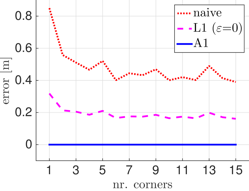
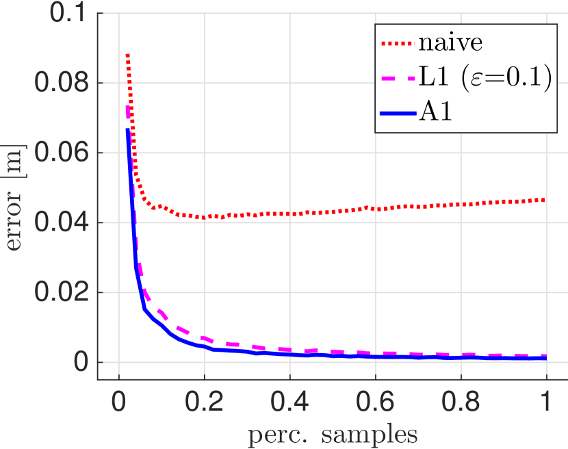
(a) error vs. # corners	(b) error vs. percentage of samples
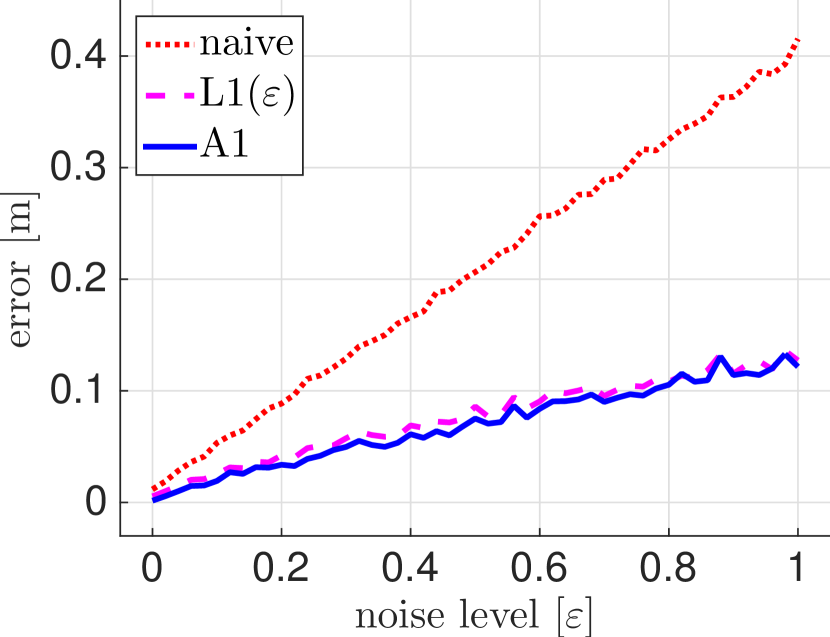
(c) error vs. noise level	(d) CPU time required

Figure 11: (a) Estimation errors committed by A1, L1, and naive, for increasing number of corners in the ground truth profile. A twin sample is acquired in each linear segment and measurements are noiseless. (b) Estimation errors from uniformly sampled noisy measurements, with increasing number of samples. (c) Estimation errors from uniformly sampled noisy measurements ($5\%$ of the depth data points) and increasing noise level. (d) CPU time required to solve L1 and A1 for increasing size $n$ of the 2D depth profile.

This section presents a Monte Carlo analysis of the reconstruction errors and timing, comparing naive, L1, and A1. Results are averaged over 50 runs, and the synthetic 2D profiles are generated as specified in the previous section.

Fig. 11(a) shows how the depth reconstruction quality is influenced by the number of corners in the ground truth profile (i.e., the sparsity of the true profile), comparing naive, L1, and A1. These results consider noiseless measurements and sample set including a twin sample in each linear region (these are the assumptions of Proposition 14). As predicted by Corollary 26, A1 recovers the original profile exactly (zero error). naive has large errors, while the L1 estimate falls between the two.

Fig. 11(b) considers a more realistic setup: since in practice we do not know where the corners are (hence we cannot guarantee to sample each linear segment of the true profile), in this case we uniformly sample depth measurements and we consider noisy measurements with $\varepsilon=0.1\text{m}$. The figure reports the estimation error for increasing number of samples. As the percentage of samples goes to 1 (100%), we sample all entries of the depth profile. We consider profiles with 3 corners in this test. The figure shows that for increasing number of samples, our approaches largely outperform the naive approach. A1 improves over L1 even in presence of noise, while the improvement is not as substantial as in the noiseless case of Fig. 11(a). Fig. 11(b) also shows that the error committed by naive does not improve when adding more samples. This can be understood from Fig. 10 and the discussion in Section VII-A1.

Fig. 11(c) considers a fixed amount of samples (5%) and tests the three approaches for increasing measurement noise. Our techniques (L1, A1), are very resilient to noise and degrade gracefully in presence of large noise (e.g., $\varepsilon=1$m).

Fig. 11(d) shows the CPU times required by L1 and A1 in 2D reconstruction problems using the cvx solver. The CPU time for naive is negligible (in the milliseconds).

VII-A3 2D mapping from sparse measurements

This section applies our approach to a 2D mapping problem from sparse measurements. We use the Stage simulator [73] to simulate a robot equipped with a laser scanner with only 10 beams, moving in a 2D scenario. The robot is in charge of mapping the scenario; we assume the trajectory to be given. Our approach works as follows: we feed the 10 samples measured by our “sparse laser” to algorithm A1; A1 returns a full scan (covering 180 degrees with 180 scans in our tests), which we feed to a standard mapping routine (we use gmapping [74] in our tests).

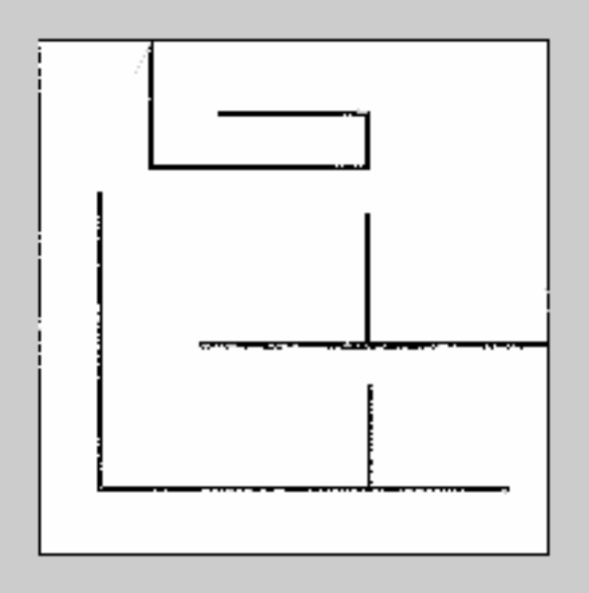
(a) full scan

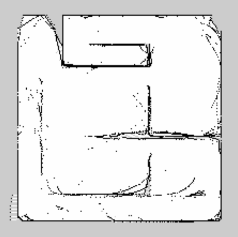
(b) naive

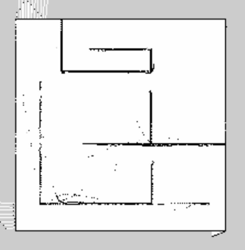
(c) A1

Figure 12: (a) Mapping using a conventional laser scanner, (b-c) Mapping using scans reconstructed by naive and A1 using 10 depth measurements.

Fig. 12 compares the occupancy grid map produced by a standard mapping algorithm based on a conventional laser scan (Fig. 12(a)), against the occupancy grid map reconstructed from our 10-beam laser. Fig. 12(b) shows the map produced from the scans estimated using naive: the map has multiple artifacts. Fig. 12(c) shows the map produced from the scans estimated using A1; the proposed technique produces a fairly accurate reconstruction from very partial information.

VII-B 3D Reconstruction: Datasets, Objective Functions and Solvers

This section introduces the 3D datasets used for the evaluation in the following sections. Moreover, it provides a statistical analysis of the performance obtained by the algorithmic variants presented in Section VI-A2, as well as the solvers presented in Section VI-B. The best performing variants and solvers will be used in the real-world examples and applications presented in Sections VII-C-VII-F.

VII-B1 Datasets

In this section we introduce the datasets we use to benchmark our 3D depth reconstruction approaches. In order to have a ground truth profile, we collected several datasets with commonly-used high-resolution depth sensors (including a Kinect and a ZED stereo camera) and use an heavily down-sampled depth image as our “sparse” depth measurements. Moreover, we created synthetic profiles for a more exhaustive evaluation.

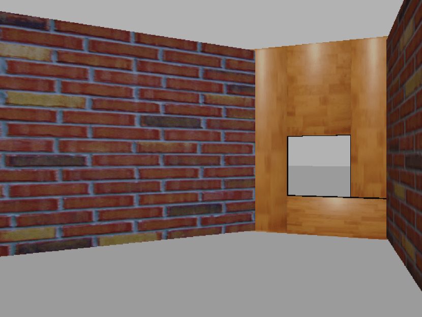
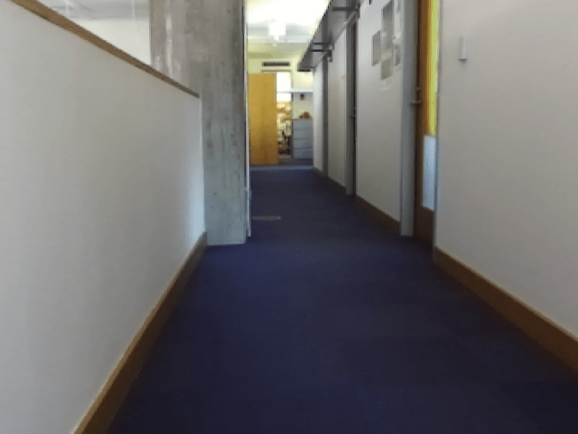
(a) Gazebo	(b) ZED
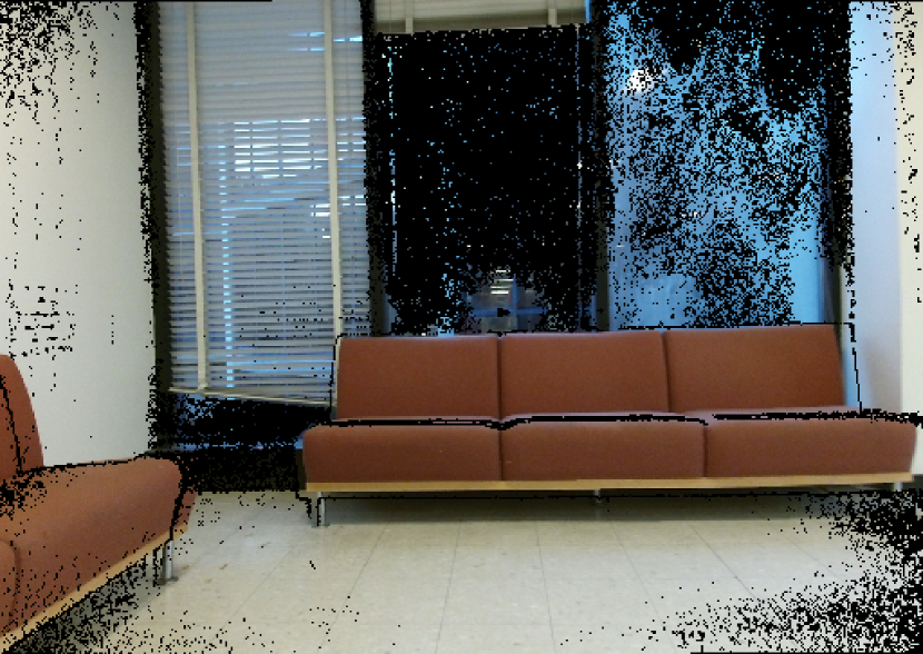
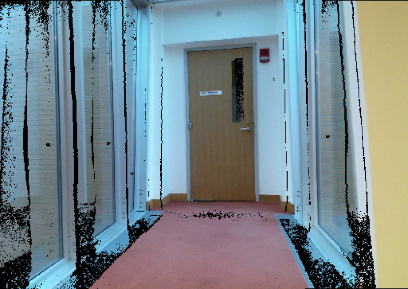
(c) Kinect	(d) Kinect

Figure 13: (a) Gazebo Simulated data. (b) ZED Stereo data. (c)-(d) Kinect data.

Our testing datasets include a dataset of randomly-generated synthetic piecewise linear depth images (denoted as PL), a simulated dataset from the Gazebo simulator [75] (denoted as Gazebo), a stereo dataset from a ZED camera (denoted as ZED), 8 datasets from a Kinect camera (denoted as K1 to K8), and the Middlebury stereo datasets [76, 77]. More specifically, Gazebo contains 20 full depth and RGB images rendered in an office-like environment from the Gazebo simulator (Fig. 13(a)). ZED includes 1000 full disparity and RBG images, collected from a ZED stereo camera mounted on a dolly, in the Laboratory of Information and Decision Systems (LIDS) at MIT (Fig. 13(b)). K1 to K8 contain odometry information, as well as depth and RGB images, collected from a Kinect sensor mounted on a dolly with wheel odometers, moving in 8 different locations at MIT, including tunnels, offices, and corridors (Fig. 13(c)-(d)). The Middlebury stereo dataset is used for the sake of benchmarking against the previous works [66, 67], which use a similar experimental setup, and includes disparity images of size 256-by-256 (each down-sampled from the original 512-by-512 images).

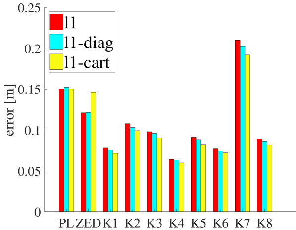
(a)

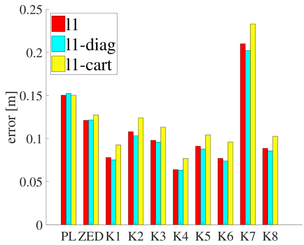
(b)

Figure 14: Comparison between three different objective functions, L1, L1diag, and L1cart, on 10 benchmarking datasets. (a) constant in L1cart is chosen as $\delta=0.1\text{m}$, (b) constant in L1cart is chosen as $\delta=0.01\text{m}$.

VII-B2 Objective Functions

In this section we compare the three objective functions discussed in Section VI-A2 for the noiseless reconstruction problem $\text{L1}_{\Delta}$. We use the cvx/MOSEK [69] solver in MATLAB in this section, to reduce numerical approximations, while we evaluate the use of other solvers (NESTA) in the next section.

Fig. 14 compares the reconstruction errors of the three different objective functions on the datasets PL, ZED, and K1-K8. The error bars show the reconstruction error for each objective functions (L1, L1diag, and L1cart), averaged over all the images in the corresponding dataset. The depth measurements are sampled from a grid, such that only $4\%$ of the pixels in the depth profiles are used. The ground truth profiles have resolution 85$\times$103 for the Kinect datasets, 96$\times$128 for the ZED dataset, and 40$\times$40 for the PL dataset.

From Section VI-A2, we recall that L1cart includes a parameter $\delta$ which prevents the denominator of some of the entries in (24) to become zero. Fig. 14(a) and Fig. 14(b) show the reconstruction errors for $\delta=0.1\text{m}$ and $\delta=0.01\text{m}$, respectively. From Fig. 14 it is clear that the accuracy of L1cart heavily depends on the choice of $\delta$, and degrades significantly for small values of $\delta$. Moreover, even for a good choice of $\delta$ (Fig. 14(a)) the advantage of L1cart over L1 and L1diag is minor in most datasets. The L1diag objective, on the other hand, performs consistently better than L1 across all datasets and is parameter-free.

We conclude that while the variants L1, L1diag, and L1cart do not induce large performance variations, L1diag ensure accurate depth reconstruction and we focus our attention on this technique in the following sections.

Extra visualizations for the L1 and L1diag formulations are provided in Appendix N and Appendix O.

VII-B3 Solvers

This section compares two solvers for $\ell_{1}$-minimization in terms of accuracy and speed. The first solver is cvx/MOSEK [69] (denoted as cvx for simplicity), a popular general-purpose parser/solver for convex optimization. The second is NESTA [18], which we adapted to our problem setup in Section VI-B. We implemented NESTA in Matlab, starting from the open-source implementation of [18]; our source code is also available at https://github.com/sparse-depth-sensing.

We compare the two solvers on the synthetic dataset PL, using the L1diag objective function. Each depth image in PL is generated randomly with a fixed number of corners (3 in our tests) and is of size $100$-by-$100$, unless otherwise specified. All depth measurements are uniformly sampled at random from the ground truth profile, and the 4 immediate neighbors (up, down, left, right) are also added into the sample sets. No noise is injected into the measurements ($\varepsilon=0$). In all tests, we set the maximum number of inner iterations to $K=10000$, the number of continuation steps to $T=5$, and the stopping criterion to $\tau=10^{-5}$ for NESTA. All data points in the plots are averaged from 50 random runs.

We start by evaluating the impact of the parameter $\mu_{f}$ on the accuracy and timing of NESTA. Fig. 15 shows the trade-off between reconstruction error and computational time for different values of $\mu_{f}$. The error is evaluated as the average mismatch between NESTA and cvx solutions. In each test, the depth samples include 5% of the pixels, uniformly chosen at random. We note that the average error is in the order of millimeters in all cases. To obtain the best trade-off between accuracy and speed, we choose $\mu_{f}=0.001$, the “elbow” point in Fig. 15. We use this value in all the following experiments.

(a)

Figure 15: Trade-off between accuracy and speed for the NESTA solver with different parameter values $\mu_{f}$. As $\mu_{f}$ decreases, NESTA produces a more accurate solution at the cost of higher computational time. The error is computed as the average mismatch between the NESTA and cvx solutions.

Fig. 16 compares the performance of cvx and NESTA for increasing number of samples, noise, and size of the depth profiles. Fig. 16(a)-(b) show the reconstruction error and computational time of the two solvers for increasing percentage of samples. Depth measurements are affected by entry-wise uniformly random measurement noise in $[-\varepsilon,\varepsilon]$; for this test we chose $\varepsilon=0.1$. Fig. 16(a) shows that the accuracy of NESTA is close to the one of cvx (the mismatch is in the order of few millimeters), while they both largely outperform Matlab’s linear interpolation (naive). Fig. 16(b) shows that NESTA is around 10x faster than cvx (as in the 2D case, the computational time of naive is negligible).

Fig. 16(c)-(d) show the reconstruction error and computational time for increasing noise level when sampling $5\%$ of the depth profile. Also in this case the errors of NESTA and cvx are very close, while NESTA remains remarkably faster. For both NESTA and cvx, the estimation error grows more gracefully with respect to the measurement noise $\varepsilon$, compared to the naive approach.

Fig. 16(e)-(f) show the reconstruction error and computational time for increasing image size. We reconstruct random profiles of size $N$-by-$N$ using 5% of samples, without adding noise. Fig. 16(e) further confirms that the error curves for cvx and NESTA are almost indistinguishable, implying that they produce reconstructions of similar quality. However, the NESTA solver entails a speed up of 3-10x, depending on the problem instance (Fig. 16(f)).

Given the significant advantage of NESTA over cvx, and since cvx is not able to scale to large profiles, we use NESTA in the tests presented in the following sections.

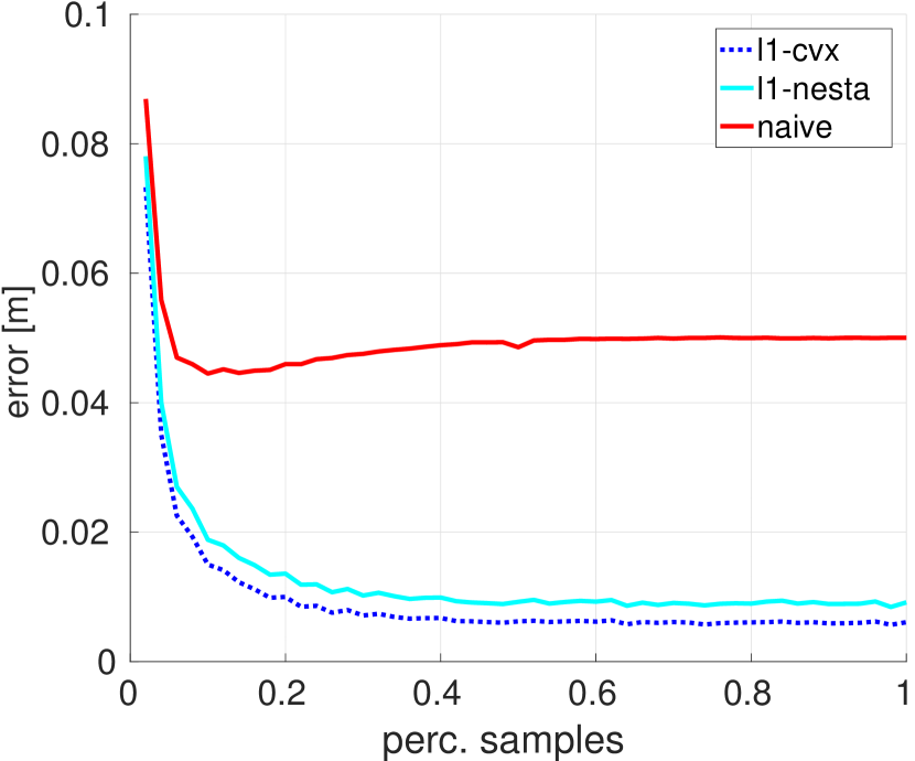
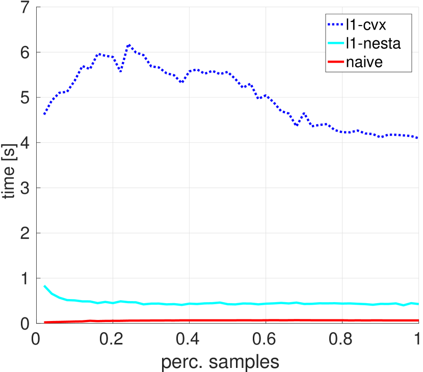
(a) error for increasing samples	(b) time for increasing samples
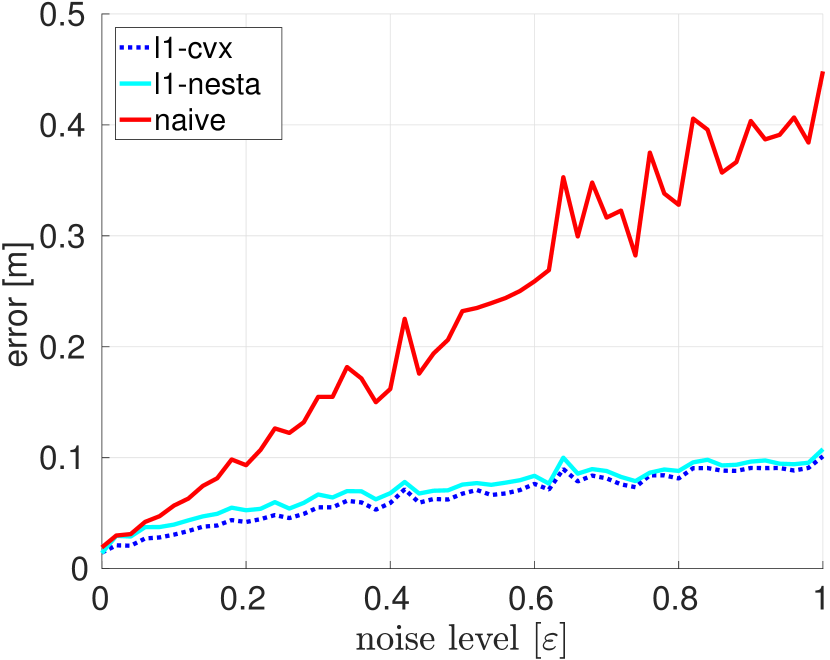
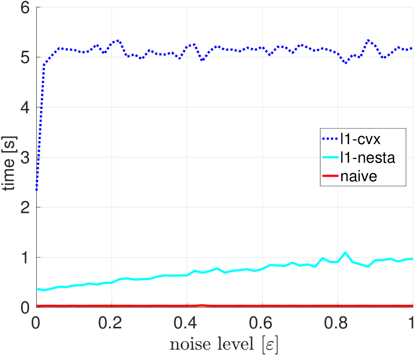
(c) error for increasing noise	(d) time for increasing noise
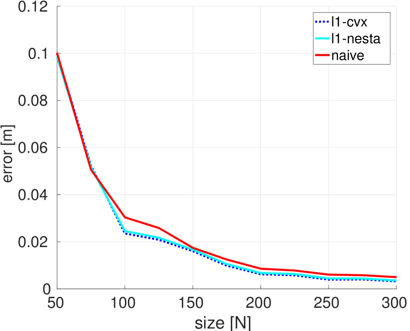
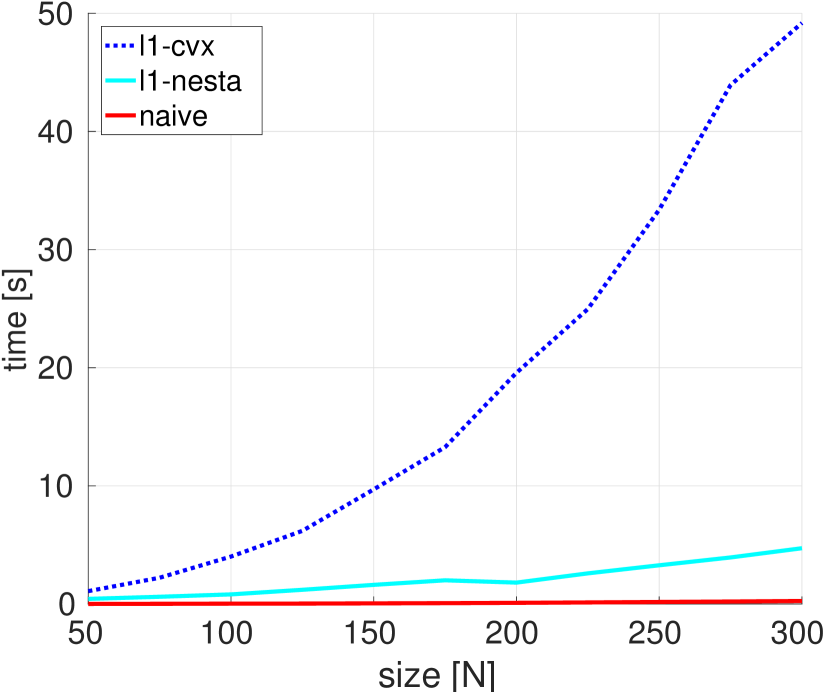
(e) error for increasing size	(f) time for increasing size

Figure 16: Comparison between NESTA ($\mu_{f}=0.001$) and cvx. Estimation errors and timing are shown for (a-b) increasing number of samples, (c-d) increasing measurement noise, (e-f) increasing size of the $N\times N$ depth profiles. NESTA achieves comparable reconstruction errors, while offering a significant speedup.

VII-C Single-Frame Sparse 3D Reconstruction

The previous section confirmed that choosing L1diag as objective function and NESTA (with $\mu_{f}=0.001$) as solver ensure the best performance. This section extends the numerical evaluation to the other 3D datasets, including Gazebo, ZED, K1-K8. For each dataset, we use L1diag to reconstruct the depth at each frame from a small subset of samples, and we compare our approach against the naive linear interpolation. In the following, we discuss typical reconstruction results, provide error statistics for different percentages of samples and noise levels, and compare L1diag against the state-of-the-art techniques proposed in [66, 67].

VII-C1 Typical Examples of 3D Reconstruction

We start by showing reconstruction examples from sparse depth measurements on the Gazebo and K1 datasets.

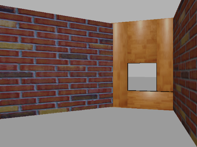
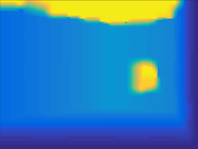
(a) Gazebo RGB image	(b) random samples	(c) reconstructed depth
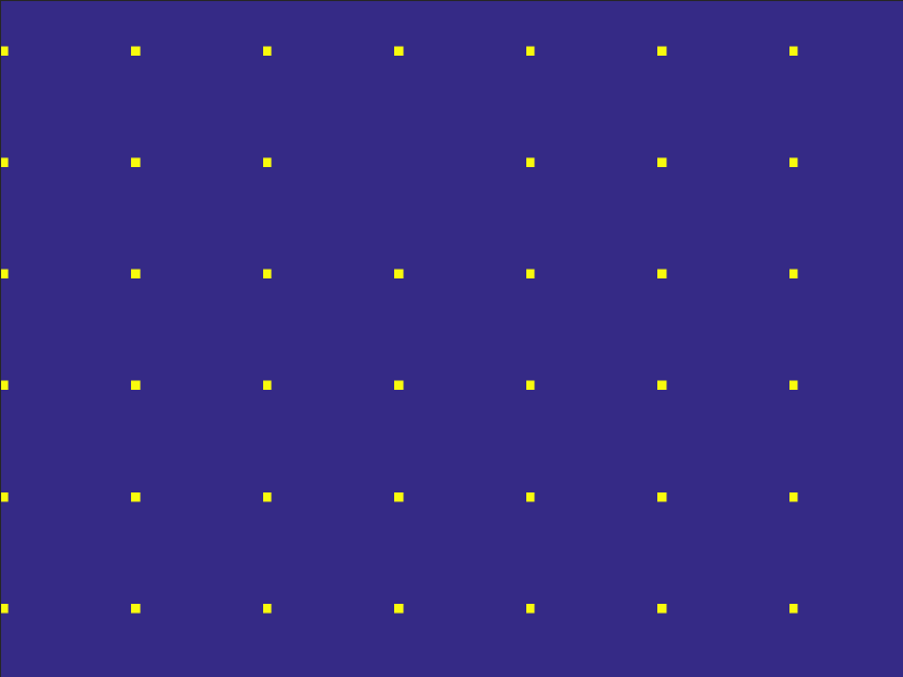
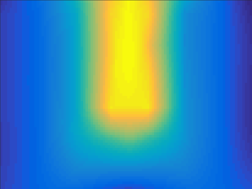
(d) Kinect RGB image	(e) grid samples	(f) reconstructed depth

Figure 17: The first row is an example of sparse depth reconstruction on Gazebo simulated data: (a) RGB image, (b) uniformly drawn sparse samples, and (c) reconstruction using L1diag. The second row is an example on Kinect K1 data: (d) RGB image, (e) sparse samples on a grid, and (f) reconstruction using L1diag.

Fig. 17(a)-(c) show an example on the Gazebo simulated dataset with uniformly random depth measurements and the reconstructed full depth profile based on these samples. The reconstructed depth image reflects the true geometry of the scene, even when we are only using 2% samples and their neighbors (total is roughly 8%). The reconstruction error in this example is 5cm.

Fig. 17 (d)-(e) shows an example on the K1 dataset, where all depth measurements fall on a regular grid. This sampling strategy resembles the output of a low-resolution depth sensor. Note that even though only a total number of 42 measurements measurements is available, the reconstructed depth image still correctly identifies the corridor and the walls. The reconstruction error in this example is 18cm.

Extra visualizations for the Gazebo and the ZED datasets are provided in Appendix N and Appendix O, respectively.

VII-C2 Statistics for 3D Reconstruction

In this section we rigorously benchmark the performance of L1diag against the naive approach, in terms of both the reconstruction accuracy and the robustness to measurement noise.

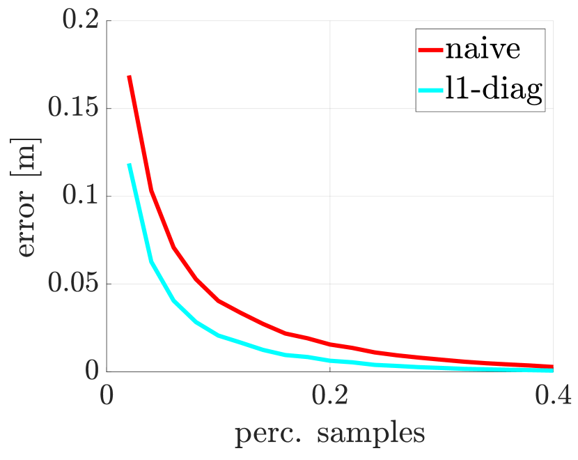
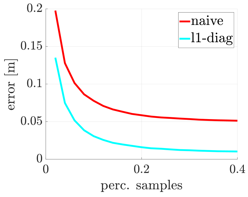
(a) Gazebo	(b) Gazebo ($\epsilon=0.1$)
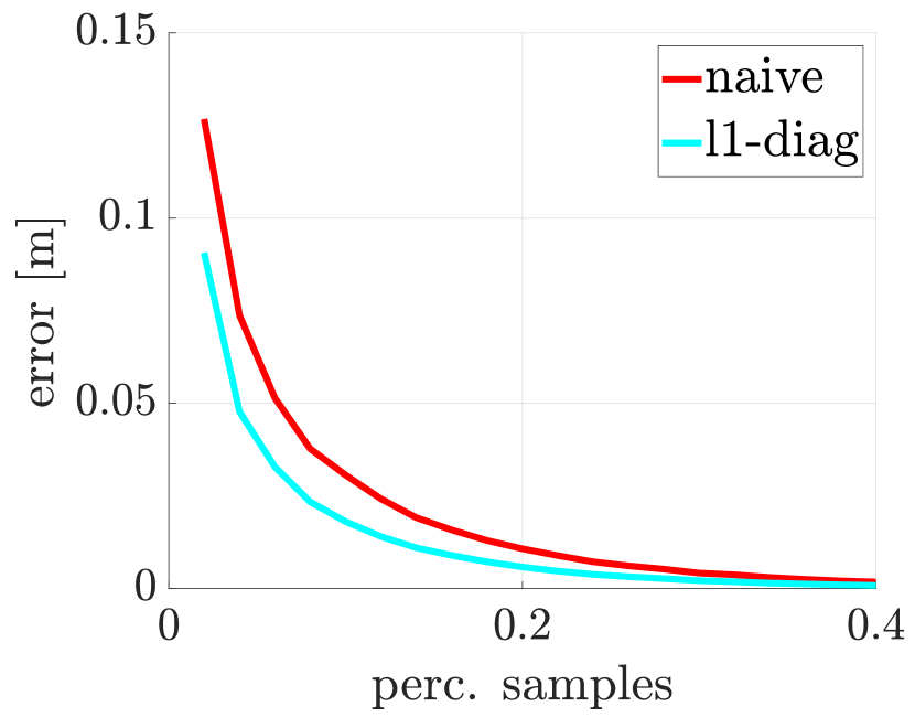
(c) ZED	(d) K1

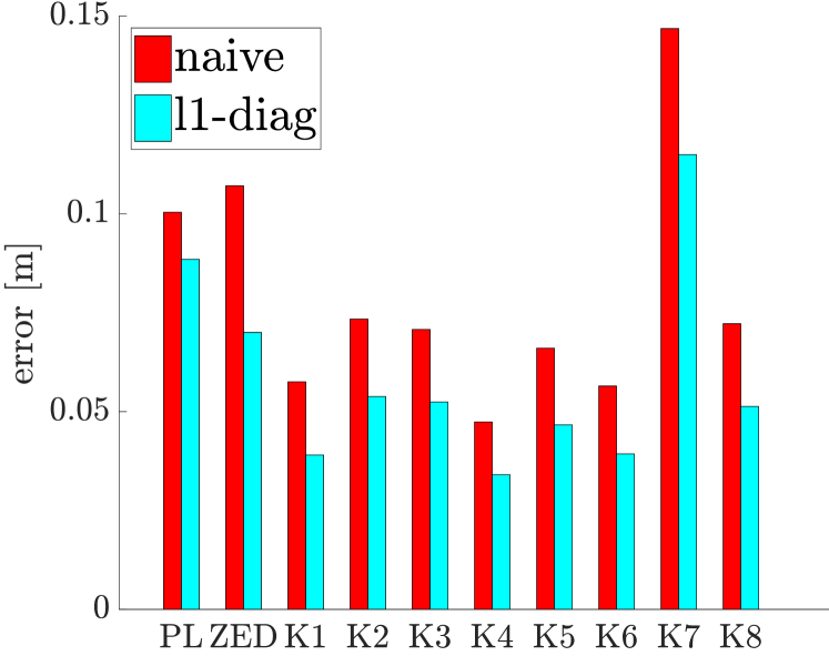
(e) comparison on all datasets

Figure 18: Reconstruction errors for increasing percentage of uniform samples, and for different datasets. (a) and (b) are reconstructions on the Gazebo dataset, using noiseless and noisy (noise bounded by $\varepsilon=0.1$m) samples, respectively. (c) reconstruction on the ZED dataset, (d) reconstruction on the K1 dataset. (e) comparison on all datasets.

Fig. 18 depicts the reconstruction errors for increasing percentages of uniformly-random samples on different datasets. Fig. 18(a) shows reconstruction from noiseless samples on the Gazebo simulated datasets, while Fig. 18(b) is the same plot except with additional pixel-wise independent Gaussian measurement noise $\varepsilon=0.1$. Fig. 18(c)-(d) show the experimental results on the ZED stereo dataset and K1 dataset. No additional noise is added to these two datasets, since the raw data is already affected by actual sensor noise. Fig. 18(e) shows the comparison between naive and L1diag over all datasets for reconstructions from 10% samples and their immediate neighbors.

From the figures it is clear that our approach consistently outperforms the naive linear interpolation in both the noiseless and noisy settings and across different datasets. The gap between L1diag and naive widens as the number of samples increases in the noisy setup, which demonstrates that our approach is more resilient to noise. In the noiseless setup, the gap shrinks as the percentage of samples converges to 100%, since in this case we are sampling a large portion of the depth profile, a regime in which the naive interpolation often provides a satisfactory approximation. L1diag produces significantly more accurate reconstruction (20-50% error reduction compared with naive) when operating below the 20%-samples regime, which is the sparse sensing setup that motivated this work in the first place.

VII-C3 Comparisons with Related Work

In this section we provide an empirical comparison of our algorithm against previous work on disparity image reconstruction from sparse measurements. Following the experimental setup used in [66, 67], we benchmark our technique in the Middlebury stereo datasets [76, 77]. Six different disparity images of size 256-by-256 (each downsampled from the original 512-by-512 images) are selected from the Middlebury dataset. We evaluate both the reconstruction accuracy and computational times for 4 different algorithms, including naive and L1diag (discussed earlier in this paper), Hawe’s CSR [66], and Liu’s WT+CT [67]. The sparse measurements are uniformly sampled from the ground truth image without noise. The same set of sparse samples are used for all 4 methods in each set of experiments. In order to allow a closer comparison with [66, 67] in this section we use the peak signal-to-noise ratio (PSNR) as a measure of reconstruction accuracy, where a higher PSNR indicates a better reconstruction. The PSNR is defined as follows, where $z$ is the reconstruction, $z^{\diamond}$ is the ground truth, and $n$ is the dimension of the vectorized profile:

$$\text{PSNR}=\frac{1}{n}\sum_{i=1}^{n}[z_{i}-z^{\diamond}_{i}]^{2}$$

Aloe
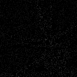
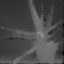
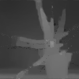
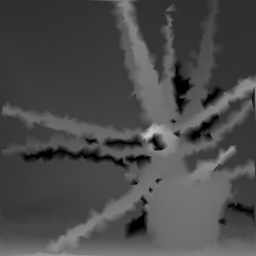
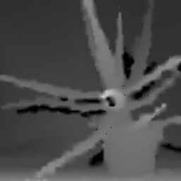
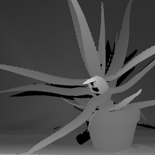
Baby
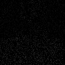
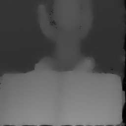
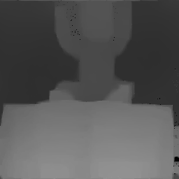
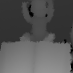
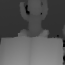
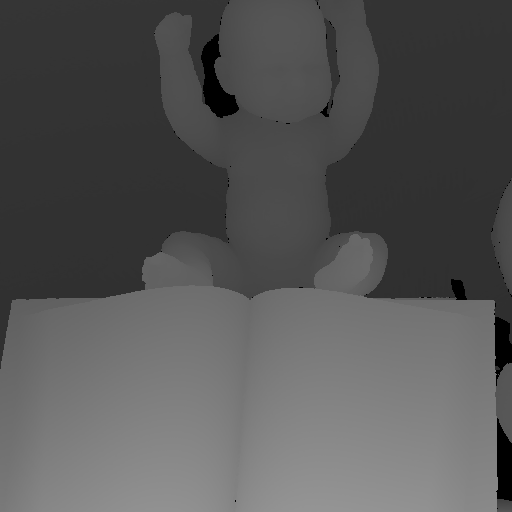
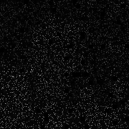
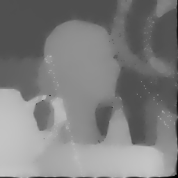
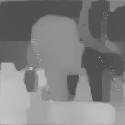
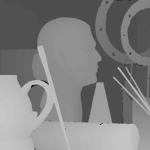
Art	5% uniform samples	CSR	WT+CT	naive	L1diag	ground truth

Figure 19: Examples of reconstruction from 5% uniformly random samples on the Middlebury disparity dataset, using 4 different algorithms: naive, L1diag, CSR [66], and WT+CT [67]. The proposed algorithm, L1diag, is able to preserve sharper boundaries and finer details, while not creating jagged edges as in naive.

To ensure a fair comparison, the initial setup (e.g., memory allocation for matrices, building a constant wavelet/contourlet dictionary) has been excluded from timing. All algorithms are initiated without warm-start, meaning that the sample image (rather than the result from naive) is used as the initial guess to our optimization problems. For L1diag, we use NESTA as solver with the same settings specified in Section VII-B3. For WT+CT, we set 100 as the maximum number of iterations, which strikes the best trade-off between accuracy and timing.

Table II reports the results of our evaluation, for each image in the Middlebury dataset (rows in the table), and for increasing number of samples (columns in the table). For each cell, we report the PSNR in dB and the time in seconds. A cell is marked as N/A if the PSNR falls below 20dB [66, 67], which indicates that either the algorithm fails to converge or that the reconstructed image is significantly different than the ground truth. Best accuracy and best timing are highlighted in bold (recall that the higher the PSNR the better).

Name	Method	PSNR (dB) / Time (s)
		(Percentage of Samples)
		0.5%	1%	5%	10%
Aloe	CSR	N/A	N/A	21.4 / 10.6	24.1 / 8.65
	WT+CT	N/A	N/A	21.9 / 19.4	24.3 / 19.5
	naive	N/A	21.6 / 0.17	24.7 / 0.14	26.0 / 0.22
	L1diag	20.6 / 14.5	21.7 / 7.02	24.9 / 3.12	26.4 / 2.06
Art	CSR	N/A	N/A	23.1 / 11.9	25.3 / 9.80
	WT+CT	N/A	N/A	25.0 / 19.8	26.7 / 19.5
	naive	21.9 / 0.15	23.5 / 0.16	26.3 / 0.17	27.7 / 0.18
	L1diag	22.5 / 11.1	23.8 / 8.86	26.6 / 3.78	27.8 / 2.23
Baby	CSR	N/A	N/A	26.6 / 10.0	31.1 / 9.11
	WT+CT	N/A	24.1 / 19.6	27.7 / 19.4	31.5 / 19.5
	naive	27.6 / 0.15	27.4 / 0.16	31.3 / 0.16	33.3 / 0.18
	L1diag	27.8 / 12.1	28.4 / 10.5	32.5 / 3.21	33.9 / 2.06
Dolls	CSR	N/A	N/A	24.3 / 13.2	26.5 / 11.0
	WT+CT	N/A	20.6 / 19.5	27.5 / 19.6	28.2 / 20.3
	naive	25.8 / 0.13	24.5 / 0.16	27.8 / 0.16	28.5 / 0.18
	L1diag	26.9 / 7.07	27.5 / 5.49	28.3 / 2.24	28.9 / 3.03
Moebius	CSR	N/A	N/A	23.6 / 11.9	26.1 / 10.5
	WT+CT	N/A	22.4 / 19.3	26.3 / 19.5	27.6 / 19.4
	naive	25.7 / 0.14	24.7 / 0.16	26.8 / 0.15	27.8 / 0.18
	L1diag	25.8 / 6.91	26.4 / 7.03	27.5 / 2.90	28.6 / 2.59
Rocks	CSR	N/A	N/A	23.1 / 11.5	25.0 / 9.15
	WT+CT	N/A	N/A	23.2 / 19.3	25.6 / 19.2
	naive	21.7 / 0.15	23.8 / 0.15	25.8 / 0.15	27.2 / 0.19
	L1diag	22.7 / 12.0	24.3 / 9.71	25.9 / 3.22	27.3 / 2.68

TABLE II: Reconstruction accuracy and computational time comparing naive, L1diag, CSR [66], and WT+CT [67]. L1diag consistently outperforms all other methods in accuracy, and performs robustly even with aggressively low number of measurements.

Our proposed algorithm L1diag consistently outperforms all other algorithms in terms of accuracy in every single experiments. In addition, L1diag is the only algorithm that ensures acceptable performance at aggressively low sampling rates (as low as 0.5%), while both [66] and [67] fail with 1% samples or fewer. L1diag is significantly faster than both [66] and [67]. For instance, L1diag takes only 50% to 10% of the computational time of WT+CT, depending on the number of samples. The naive interpolation is very fast, but produces worse reconstruction than L1diag. We noticed that in these tests we can achieve even faster runtime for L1diag by using a larger parameter $\mu_{f}$ without suffering much loss in accuracy. For instance, for $\mu_{f}=0.1$, the average computation time with 5% samples reduces from around 3s to around 2s, while the PSNR remains at roughly the same level and still outperforms other approaches.

For a visual comparison, Fig. 19 reports some examples of the reconstructed disparity images for each of the compared techniques. The proposed algorithm, L1diag, is able to preserve sharp boundaries and fine details, while avoiding the creation of jagged edges as in naive.

VII-D Multi-Frame Sparse 3D Reconstruction

In the previous Section VII-C we focused on depth reconstruction from sparse measurements of a subset of pixels in a single frame. However, when odometry information is available (e.g., from a wheel odometer on ground vehicles, or from inertial measurement units on aerial robots), it is possible to combine sparse measurements across multiple consecutive frames in a time window in order to improve the reconstruction. More precisely, at every frame $t$, we use the samples collected at frames $t-H,t-H+1,\ldots,t$ (where $H$ is a given horizon) to improve the quality of the 3D reconstruction. Since each depth sample collected at time $t^{\prime}<t$ can be associated to a 3D point in the reference frame of the sensor at time $t^{\prime}$, we use the relative pose between $t^{\prime}$ and $t$ to express the 3D point in the reference frame at time $t$, hence obtaining an extra measurement at time $t$. This way, we accumulate all measurements from the past frames in the time window, and we leverage this larger set of measurements to improve the depth reconstruction at time $t$. Note that we assume the environment is static and the odometry is accurate within a short time window. To some extent, we can model odometric errors by associating larger noise levels $\varepsilon$ to samples acquired at older frames.

In this section, we demonstrate this idea on the K1-K8 datasets, where the odometry information is available and can be considered reliable over a short temporal window.

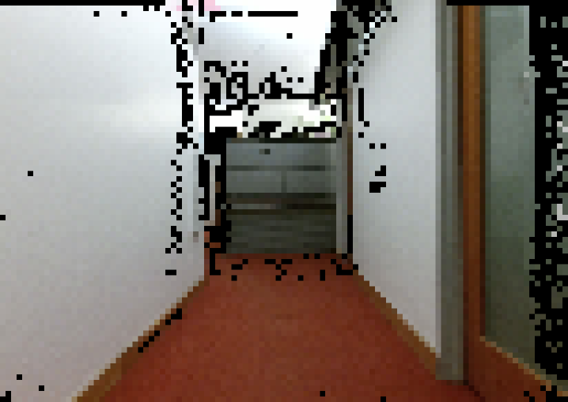
(a) environment

(b) samples collected from 10 frames

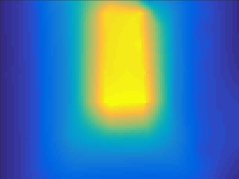
(c) reconstructed depth

Figure 20: (a) registered RGB image from the Kinect sensor, (b) depth samples collected across multiple time frames, (c) depth reconstruction using samples collected over a receding time horizon. With more samples collected from several frames, the temporal reconstruction becomes more accurate (e.g., sharper at edges) compared to the reconstruction using samples from a single frame.

VII-D1 Typical Examples of Multi-Frame 3D Reconstruction

Fig. 20 shows an example of multi-frame reconstruction. Fig. 20(a) is an RGB image (registered with the depth image, and thus missing some pixels for which the depth is not available). Fig. 20(b) shows the depth measurements collected over a temporal window of 10 frames. Fig. 20(c) shows the reconstructed depth profile from all the measurements collected in a receding time horizon. When compared against the single-frame counterpart in Fig. 17(e), it can be observed that the additional measurements contribute to making the depth profile sharper and more accurate. The reconstruction error with data from 10 frames is 26cm, as opposed to 39cm when using only one single frame.

VII-D2 Statistics for Multi-Frame 3D Reconstruction

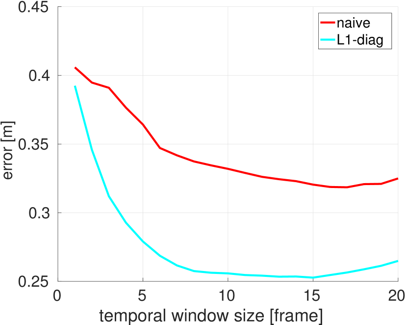
(a)

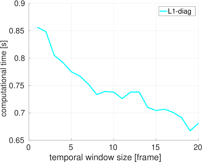
(b)

Figure 21: The two figures show error and timing statistics against increasing horizon size for temporal reconstruction. With more samples collected, the accuracy increases and the computational decreases (due to more constraints in the optimization problem). However, when the horizon size is very large, the error rises due to accumulated odometry error.

Fig. 21 reports the results of the comparison between the performance of the multi-frame reconstruction (labeled as L1diag, with $\varepsilon=0$) and the baseline naive (linear interpolation). In both approaches, we use all samples collected over a receding horizon as input to the reconstruction. The results in the figure are obtained on the K1 dataset, and each data point in the plot is averaged over 910 images. From each frame only 18 depth measurements are collected (the full image has $2236$ pixels), and the samples fall on a regular grid.

Fig. 21(a) reports the estimation errors for naive and L1diag for increasing time windows. It can be observed that L1diag consistently outperforms naive. The best performance is achieved for a temporal window of 15 frames (approximately 2 seconds), with an average reconstruction error of $25\text{cm}$, while the average error for the single-frame reconstruction (i.e., 1-frame window) is $39\text{cm}$, which is 56% higher. The error curve of Fig. 21(a) has a minimum (15-frame horizon), and then starts increasing for longer horizons. This phenomenon can be attributed to the odometry drift (i.e., the accumulation of odometry errors) over time. The odometric error cannot be considered negligible over a long time horizon, hence inducing larger noise in the samples and degraded reconstruction performance.

Fig. 21(b) shows the computational time for our algorithm L1diag using NESTA. The runtime decreases with the length of the temporal horizon. This is due to reduction of the search space in the optimization problem, thanks to additional constraints induced by the measurements at the past frames.

VII-E Data Compression of 3D Profiles

Another major application of the proposed algorithms lies in bandwidth-limited robot-server communication. Instead of having to transmit the entire depth profile from the robot to a remote server, the basic idea is that the robot can transmit a subset of the pixels and the server can then use the reconstruction algorithms discussed in this paper to retrieve the full profile. A major difference with respect to the setup discussed in the previous sections, is that in compression problems, the robot has access to the full profile, hence it can use a more clever sampling strategy and improve the reconstruction results. For instance, the robot can sample the edges (and theirs neighbors) in the depth profile, which, according to Proposition 8, are sufficient to reconstruct the original 3D depth profile exactly.

In this section, we show empirically that by sending only the depth data along the edges (extracted either from the RGB images or the depth profiles), we can significantly reduce the required communication bandwidth, at a minor loss of accuracy. We measure the amount of data compression using the data rate saving, defined as

$$\text{data rate saving}=1-\frac{\text{compressed data rate}}{\text{uncompressed data rate}}.$$ (29)

We demonstrate the compression technique on both the Gazebo and the ZED datasets. We separate the discussions regarding edge extraction from RGB images and from the depth profiles. This is due to the fact that they have different pros and cons, and thus can be applied in different scenarios.

VII-E1 Sampling Depth Edges

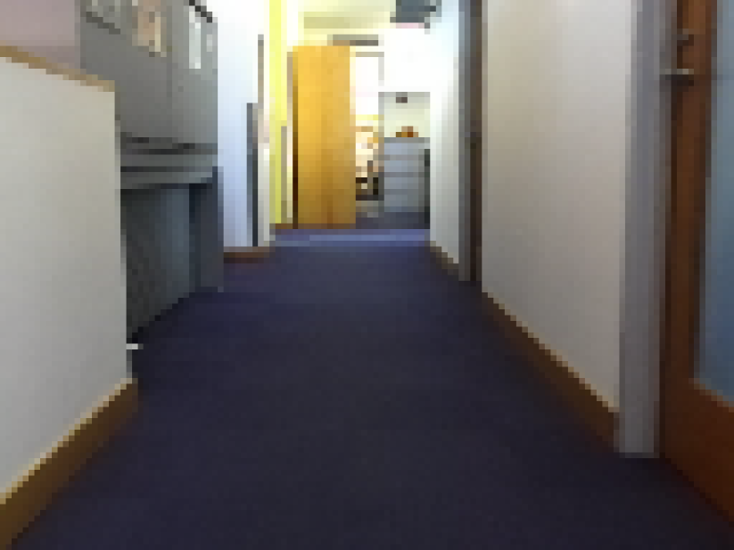
(a) RGB image

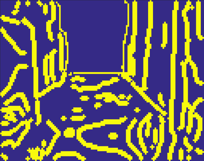
(b) depth edges

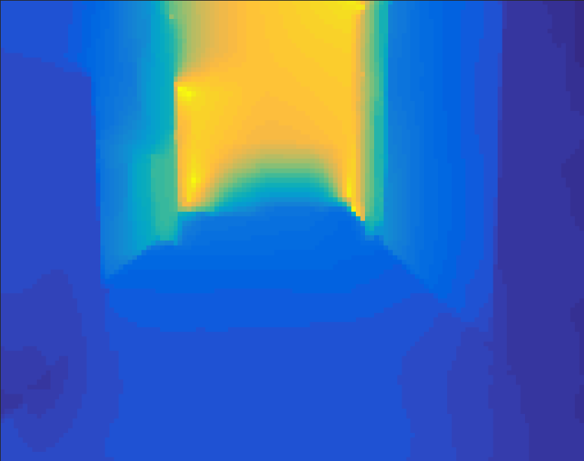
(c) reconstruction

Figure 22: An example of data compression using the edges in the depth profile: (a) RBG image, (b) edges in the depth profile, (c) depth profile reconstructed using L1diag. Spurious edges appear due to distortions in the full stereo disparity images.

Fig. 22 presents an example of reconstruction based solely on samples along the depth edges (and their neighbors). In this case, the robot only transmits the neighborhood of the pixels for which the depth curvature (along the horizontal or vertical directions) is larger than a given threshold; a large threshold implies that less pixels are transmitted as edges, at a potential loss of reconstruction accuracy. We use the Canny edge detector [78] (implemented in Matlab, with default parameters) to extract the edges from the depth image. We compare the reconstructed depth profile (at the server) with the full profile from the ZED stereo camera, and show the statistics in Fig. 23.

Fig. 23(a) compares the reconstruction errors of the naive linear interpolation and the proposed L1diag approach with respect to the full ZED depth profile. L1diag achieves almost half of the reconstruction error of naive. In addition, the error is very small (in the order of few centimeters), implying almost exact recovery from samples along depth edges. On the other hand, Fig. 23(b) shows that the data rate saving, defined in (29), is around 70-85%. This implies that the same bandwidth is now able to accommodate 3x-6x more communication channels.

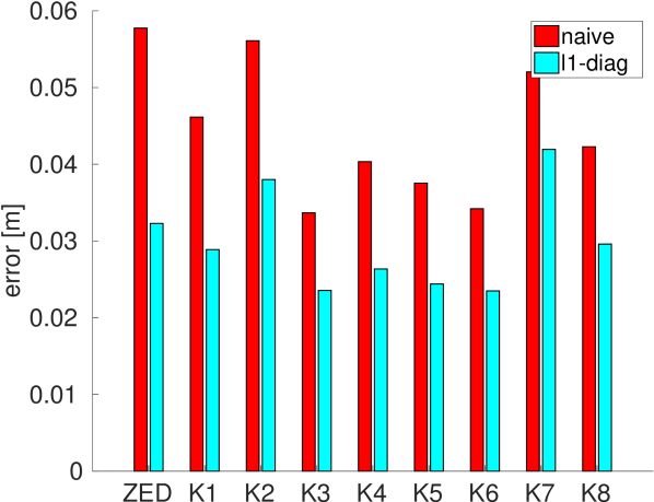
(a)

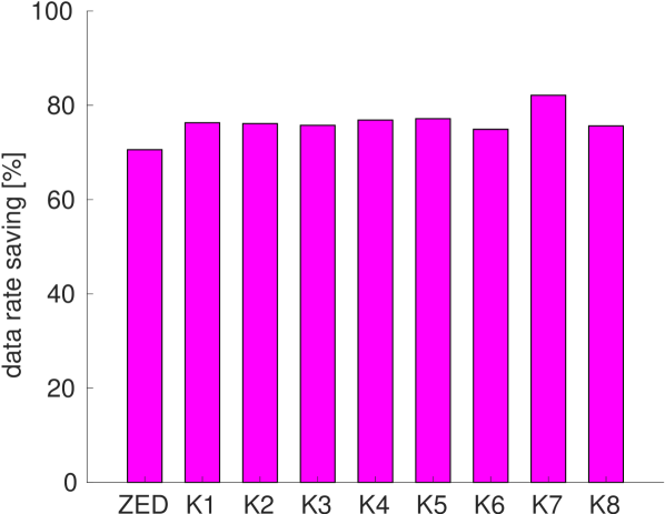
(b)

Figure 23: (a) reconstruction errors and (b) data rate saving for the case when only depth edges are transmitted to the server.

Note that the full depth profile from stereo cameras suffers from distortion and is error-prone in regions with small intensity gradients, resulting in many spurious edges in the original ZED image. For instance, in Fig. 22(b), unnecessary edges appear on the (flat) ground as well as on the walls. These unwanted edges will be sent to the server, thus being the result of stereo reconstruction errors rather than actual depth discontinuities, hence preventing further data compression. This motivates us to consider samples along the RGB (instead of the depth) edges, as discussed below.

VII-E2 Sampling RGB Edges

(a) RGB image

(b) RGB edges

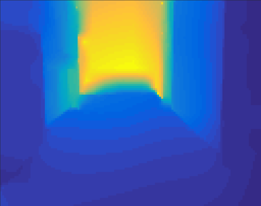
(c) reconstruction

Figure 24: An example of data compression using the depth along the edges in the RGB image: (a) RBG image, (b) edges in the RGB image, (c) depth profile reconstructed using L1diag.

In this section, we discuss the advantage of using depth sampled along the RGB edges (pixels with large image intensity gradients), over the depth edges used in the previous section. Similar to the depth edge extraction, we use the Canny algorithm, this time applied to the RBG image. In most scenarios, depth discontinuities are reflected in appearance discontinuities. This implies that the RGB edges are usually a superset of the real edges in the scene. By extracting RGB edges, our goal is to avoid unnecessary and erroneous edges as seen in Fig. 22(b), and thus improve accuracy and data rate saving. We remark that these considerations are due the fact that the full depth profile (collected by the robot) is noisy, making tricky to distinguish actual depth discontinuities from pixel noise.

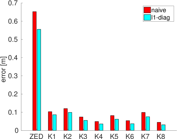
(a)

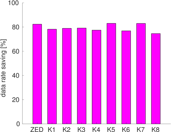
(b)

Figure 25: When only depth data along RGB edges are transmitted, the reconstruction error is minimal except for the ZED dataset. This is because of the fact that disparity images provided by the ZED stereo camera are noisy and have undesirable edges, due to inherent depth distortion of stereo-vision. In other words, edges extracted from the depth images and from the RGB images are not consistent. (a) reconstruction error. (b) data rate saving.

Fig. 24 shows the same example as in Fig. 22, but with edges extracted from the RGB image. More specifically, Fig. 24(b) shows the depth measurements along the RGB edges extracted from Fig. 24(a), and Fig. 24(c) is the reconstruction result. We observe a smaller and cleaner set of edges.

The reconstruction error and data rate saving statistics, for the case in which only RBG edges are transmitted to the server, are shown in Fig. 25. Note that L1diag still consistently outperforms the baseline naive on every single datasets, although they both perform poorly on the ZED stereo datasets. As discussed before, the disparity images from the ZED stereo camera suffer from distortion (see Fig. 22(b) for example). In other words, the ground truth depth itself is highly noisy. Therefore, even if the reconstructed depth may match more accurately the actual geometry of the 3D scene (since L1diag is capable of filtering our some of the noise), we would not expect a decline in the error metric, which is computed with respect to the ZED profile. Fig. 25(b) shows that, as expected, the use of RBG edges implies a slightly larger data rate saving, compared to the depth edges of Fig. 22(b).

Extra visualizations, comparing reconstruction from sparse samples and from RGB edges for the Gazebo and the ZED datasets, are provided in Appendix N and Appendix O.

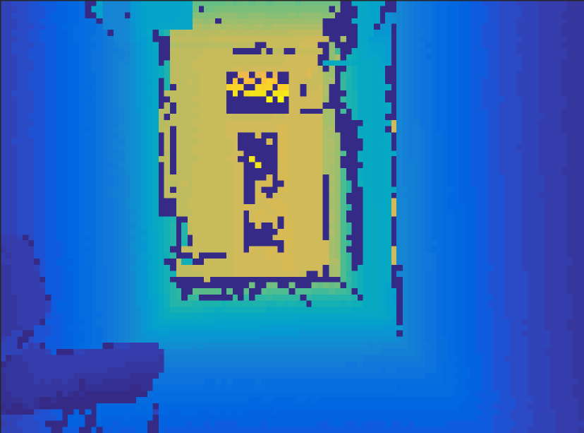
(a) 72-by-103 depth image

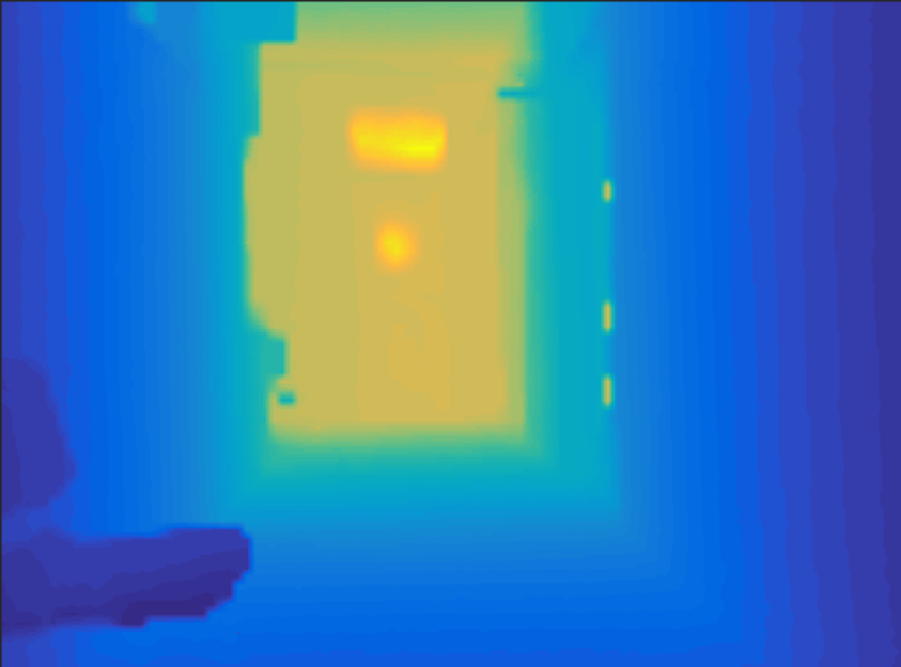
(b) up-scaled 359-by-512 image

Figure 26: Super-resolution depth imaging. The up-scale factor is 24.79 in this example.

VII-F Super-dense 3D Reconstruction and Super-resolution Depth Imaging

In this section, we demonstrate that our algorithm can also be applied to super-resolution depth imaging. Super-resolution imaging attempts to algorithmically increase the resolution of a given depth profile. This is fundamentally the same as viewing an input full depth profile as measurements sampled from a higher-resolution “ground truth” and do reconstruction based on such measurements. An example is shown in Fig. 26 using Kinect data. The original profile, in Fig. 26(a), has a resolution of 72-by-103 and many missing pixels (due to Kinect sensor noise). Fig. 26(b) shows the reconstructed, or in other words up-scaled, depth image. The size of the reconstructed depth image is 359-by-512, and thus has an up-scale factor of 24.79. Roughly speaking, 1 depth pixel in the input profile translates to a 5-by-5 patch in the up-scaled depth profile. Note that all missing pixels (including the legs of the chair in Fig. 26(a)) are smoothed out.

VIII Conclusion and Future Work

In this work, we propose a new approach to recover dense 2D and 3D depth profiles from sparse and incomplete depth measurements. As a first contribution, we formulate depth reconstruction as the problem of finding a profile that has the sparsest second-order derivative, i.e., the least amount of corners and edges, while matching the given measurements. The problem itself is NP-hard, hence we relax it to a convex $\ell_{1}$-minimization problem with $\ell_{\infty}$-norm constraints.

Our second contribution is a theoretical analysis that establishes precise conditions under which the dense depth profile can be recovered from sparse samples. Even in the case in which exact recovery is not possible, we provide error bounds on the estimated profile and discuss its sensitivity to measurement noise in both 2D and 3D problems.

As a third contribution, we present several algorithmic variants to recover the depth profile, each one resulting in a convex optimization problem. To further accelerate these algorithms, we discuss how to adapt NESTA, a first-order method for nonsmooth optimization, to our problem setup.

The fourth contribution is an extensive experimental evaluation on both synthetic and real data. The experimental results show that our algorithms are able to reconstruct a dense depth profile from an extremely low number of measurements (e.g., we can recover a $100$-by-$100$ depth profile from 40 measurements), are robust to measurement noise, and are able to scale to large profiles. The capability of properly modeling measurement noise enables a performance boost with respect to interpolation-based approaches. We demonstrated the proposed approach in many applications, including 2D mapping, single-frame and multi-frame 3D depth reconstruction from sparse measurements, 3D depth profile compression and decompression, as well as super-resolution depth imaging.

As future work, we plan to further accelerate our algorithms using parallel computing (e.g., GPU). We would also like to apply the proposed algorithm to distributed mapping in bandwidth-limited multi-robot systems. In addition, we are interested in developing motion planning algorithms that can pro-actively guide the depth sampling process and further improve the reconstruction results.

Appendix A Some Useful Lemmas

We introduce some technical lemmas which simplify the derivations in the following sections.

Lemma 27 (Null space of $A$).

Consider the sparse sampling matrix $A\in{{\mathbb{R}}^{m\times n}}$. The null space of $A$ is spanned by the rows of the matrix $N\doteq{\mathbf{I}}_{\overline{{\cal M}}}\in{{\mathbb{R}}^{\bar{m}\times n}}$ (with $\bar{m}\doteq n-m$). Moreover, the action of the matrix $N$ on a vector $v$ and on a matrix $V$ of suitable dimensions is such that $Nv=v_{\overline{{\cal M}}}$ and $NV=V_{\overline{{\cal M}}}$.

Proof.

Denote the $i$-th standard basis vector as $e_{i}$. Each row of $A\in{{\mathbb{R}}^{m\times n}}$ is equal to $e_{i}^{\mathsf{T}}$ for some $i\in{\cal M}$, hence $A$ has rank $m$. Since the sets ${\cal M}$ and $\overline{{\cal M}}$ are disjoint and are such that ${\cal M}\cup\overline{{\cal M}}=\{1,\ldots,n\}$, it follows that $AN^{\mathsf{T}}=0$ (entries of $AN^{\mathsf{T}}$ have the form $e_{i}^{\mathsf{T}}e_{j}$ which is zero for ${\cal M}\ni i\neq j\in\overline{{\cal M}}$) and $N^{\mathsf{T}}$ has rank $\bar{m}=n-m$. This proves that the rows of $N$ span the null space of $A$. Since each row of $N$ is $e_{j}^{\mathsf{T}}$ for some $j\in\overline{{\cal M}}$, the claims $Nv=v_{\overline{{\cal M}}}$ and $NV=V_{\overline{{\cal M}}}$ easily follow. ∎

Lemma 28 (Symmetric Tridiagonal Toeplitz matrix).

Let $T$ denote a symmetric tridiagonal Toeplitz matrix with diagonal entries equal to $-2$ and off-diagonal entries equal to $1$:

$$T\doteq\left[\begin{array}[]{cccccc}-2&1&0&0&\ldots&0\\ 1&-2&1&0&\ldots&0\\ 0&1&-2&-1&\ldots&0\\ \vdots&\ddots&\ddots&\ddots&\ddots&0\\ 0&\ldots&0&0&1&-2\\ \end{array}\right]$$ (30)

Then the following claims hold:

1. $T$ is invertible;

2. all the entries in the first and in the last column of $T^{-1}$ are negative and have absolute value smaller than 1;

3. let $v\in{{\mathbb{R}}^{n}}$ be defined as $v\doteq[1\;0\;\ldots\;0\;1]^{\mathsf{T}}$, then $T^{-1}v=-{\mathbf{1}}$.

Proof.

Invertibility follows from [79, Corollary 4.2], which also reports the explicit form of the inverse of a Toeplitz matrix. We report the inverse here, tailoring it to our matrix. For the $n\times n$ Toeplitz matrix $T$ in eq. (30), the entry in row $i$ and column $j$ of $T^{-1}$ is:

$$(T^{-1})_{ij}=\left\{\begin{array}[]{ll}(-1)^{2i-1}\frac{i(n-j+1)}{n+1}&\text{if }i\leq j\\ (-1)^{2j-1}\frac{j(n-i+1)}{n+1}&\text{if }i>j\end{array}\right.$$ (31)

By inspection one can see that the first column ($j=1$) and the last column $j=n$ are all negative and have absolute value smaller than 1. The last claim can be proven by observing that $T{\mathbf{1}}=-v$ and the matrix is invertible. ∎

Lemma 29 (Null Space of D).

Given a 2^nd-order difference operator $D\in{{\mathbb{R}}^{(n-2)\times n}}$, defined as in (6), the null space of $D$ is spanned by the following vectors:

$$v_{1}={\mathbf{1}}_{n}\qquad v_{2}=[1\;2\;\ldots\;n]^{\mathsf{T}}$$ (32)

Proof.

By inspection one can see that $Dv_{1}=Dv_{2}={\mathbf{0}}$. Moreover, the rank of $D$ is $n-2$ and $v_{1}$ and $v_{2}$ are two linearly independent vectors, which proves the claim. ∎

Appendix B Proof of Proposition 7

In this appendix we prove that in 2D depth reconstruction problems, if we sample only the corners of the profile (and the first and the last entry), then $C_{\text{er}}=1$. Moreover, we prove that if we sample the corners and their neighbors we have $C_{\text{er}}=0$. We start by rewriting Equation 13 in a more convenient form. Using Lemma 27, we know that $N(D_{\cal J})^{\mathsf{T}}=[D^{\mathsf{T}}]_{\overline{{\cal M}},{\cal J}}$. In words, $D_{\cal J}$ selects the rows of $D$ at indices ${\cal J}$, or equivalently the columns of $D^{\mathsf{T}}$. Similarly the multiplication by $N$ selects the rows of $D^{\mathsf{T}}$ at indices $\overline{{\cal M}}$. Similarly, $N(D_{\cal I})^{\mathsf{T}}=[D^{\mathsf{T}}]_{\overline{{\cal M}},{\cal I}}$. Using these relations, Equation 13 simplifies to:

$$C_{\text{er}}=\|([D^{\mathsf{T}}]_{\overline{{\cal M}},{\cal J}})^{\dagger}[D^{\mathsf{T}}]_{\overline{{\cal M}},{\cal I}}\|_{\infty\rightarrow\infty}<1$$ (33)

Since ${\cal I}\cup{\cal J}=\{1,\ldots,n\}$, it is clear that $[D^{\mathsf{T}}]_{\overline{{\cal M}},{\cal J}}$ and $[D^{\mathsf{T}}]_{\overline{{\cal M}},{\cal I}}$ are disjoint sets of columns of the matrix $[D^{\mathsf{T}}]_{\overline{{\cal M}}}$.

Let us start with the first claim: $C_{\text{er}}=1$ whenever we sample the corners, the first, and the last entry of a profile. We will make an extensive use of the structure of the matrix $D^{\mathsf{T}}$ which is the transpose of Equation 6. To give a more intuitive understanding of the proof we provide a small example of $D^{\mathsf{T}}$ with $n=12$:

(34)

The matrix $[D^{\mathsf{T}}]_{\overline{{\cal M}}}$ is obtained from $D^{\mathsf{T}}$ after removing the rows at indices in the sample set ${\cal M}$: these “deleted” rows are shown in gray in Equation 34. In particular, according to the assumptions of the first claim of Proposition 7, ${\cal M}$ contains the first and the last sample (first and last row in $D^{\mathsf{T}}$) plus intermediate rows corresponding to corners (two intermediate gray rows in the figure). Now we note that the matrix $[D^{\mathsf{T}}]_{\overline{{\cal M}},{\cal I}}$ selects the columns with indices in ${\cal I}$ from $[D^{\mathsf{T}}]_{\overline{{\cal M}}}$. In figure, the columns that form $[D^{\mathsf{T}}]_{\overline{{\cal M}},{\cal I}}$ are shown in dashed red boxes. The position of these columns is dictated by the position of the corners, hence if the $i$-th row corresponds to a corner, than column $i\!-\!1$ belongs to ${\cal I}$.

Three considerations are in order now. First, the matrix $[D^{\mathsf{T}}]_{\overline{{\cal M}},{\cal J}}$ is a block-diagonal square matrix with diagonal blocks being Toeplitz matrices (cf. with Equation 30). Second, the matrix is invertible (follows from the first claim of Lemma 28). Third, the matrix $[D^{\mathsf{T}}]_{\overline{{\cal M}},{\cal I}}$ only contains 0 and 1 in suitable positions. Therefore, the matrix $([D^{\mathsf{T}}]_{\overline{{\cal M}},{\cal J}})^{\dagger}[D^{\mathsf{T}}]_{\overline{{\cal M}},{\cal I}}=([D^{\mathsf{T}}]_{\overline{{\cal M}},{\cal J}})^{-1}[D^{\mathsf{T}}]_{\overline{{\cal M}},{\cal I}}$ has the following block structure:

$$\left[\begin{array}[]{c}T_{1}^{-1}\left[\begin{array}[]{ccccc}0&0&\ldots&0&0\\ \vdots&\vdots&\vdots&\vdots&\vdots\\ 1&0&\ldots&0&0\end{array}\right]\\ T_{2}^{-1}\left[\begin{array}[]{ccccc}1&0&\ldots&0&0\\ \vdots&\vdots&\vdots&\vdots&\vdots\\ 0&1&\ldots&0&0\end{array}\right]\\ \vdots\\ T_{K}^{-1}\left[\begin{array}[]{ccccc}0&0&\ldots&0&1\\ \vdots&\vdots&\vdots&\vdots&\vdots\\ 0&0&\ldots&0&0\end{array}\right]\\ \end{array}\right]=\left[\begin{array}[]{c}T_{1}^{-1}R_{1}\\ T_{2}^{-1}R_{2}\\ \vdots\\ T_{K}^{-1}R_{K}\\ \end{array}\right]$$ (35)

where $T_{1},\ldots,T_{K}$ are Toeplitz matrices of suitable dimensions and each $R_{i}$ contains at most two nonzero elements (equal to 1) in the first and the last row. Since for a matrix $M$, $\|M\|_{\infty\rightarrow\infty}$ is the maximum of the $\ell_{1}$-norm of each row, we only need to demonstrate that the maximum $\ell_{1}$-norm of the rows of $T_{i}^{-1}R_{i}$ is no larger than 1 for all $i$. The action of $R_{i}$ on $T^{-1}_{i}$ is to select the first and/or the last column of $T_{i}^{-1}$ (depending on where the 1 appears). For instance, $T^{-1}_{1}R_{1}$ is zero everywhere, except the fist column which is equal to the last column of $T^{-1}_{1}$. From Lemma 28(ii) we know that the entries in the first column have magnitude smaller than 1 hence it follows that $\|T^{-1}_{1}R_{1}\|_{\infty\rightarrow\infty}<1$. A similar argument holds for the last column, hence $\|T^{-1}_{K}R_{K}\|_{\infty\rightarrow\infty}<1$. For the intermediate blocks $T^{-1}_{i}R_{i}$, $1<i<K$, it can be seen that $\|T^{-1}_{i}R_{i}\|_{\infty\rightarrow\infty}=\|T^{-1}_{i}v\|_{\infty}$, with $v\doteq[1\;0\;\ldots\;0\;1]^{\mathsf{T}}$; this follows from the fact that $R_{i}$ selects the first and the last columns of $T^{-1}_{i}$ which have negative entries due to Lemma 28(ii). Using Lemma 28(iii) we know that $T^{-1}v=-{\mathbf{1}}$, from which it follows $\|T^{-1}_{i}R_{i}\|_{\infty\rightarrow\infty}=\|T^{-1}_{i}v\|_{\infty}=1$. This proves the first claim.

The proof of the second claim ($C_{\text{er}}=0$ when we sample the corners and their neighbors) is much simpler. Sampling the neighbors corresponds to deleting the rows contiguous to each “corner” from $D^{\mathsf{T}}$. From Equation 34 the reader can easily see that this choice makes $[D^{\mathsf{T}}]_{\overline{{\cal M}},{\cal I}}={\mathbf{0}}$, which in turns implies $C_{\text{er}}\doteq\|([D^{\mathsf{T}}]_{\overline{{\cal M}},{\cal J}})^{\dagger}[D^{\mathsf{T}}]_{\overline{{\cal M}},{\cal I}}\|_{\infty\rightarrow\infty}=0$. ∎

Appendix C Proof of Proposition 8

In this appendix we prove that in 3D depth reconstruction problems, if we sample the edges and the corresponding vertical and horizontal neighbors, then:

$$C_{\text{er}}\doteq\|(N(\Delta_{\cal J})^{\mathsf{T}})^{\dagger}N(\Delta_{\cal I})^{\mathsf{T}})\|_{\infty\rightarrow\infty}=0$$ (36)

which implies exact recovery of the original depth profile according to Proposition 6. As in Appendix B we rewrite the condition (36) as:

$$C_{\text{er}}=\|([\Delta^{\mathsf{T}}]_{\overline{{\cal M}},{\cal J}})^{\dagger}[\Delta^{\mathsf{T}}]_{\overline{{\cal M}},{\cal I}}\|_{\infty\rightarrow\infty}=0$$ (37)

The proof proceeds along the same line of the proof of the second claim in Proposition 7. By observing the structure of $\Delta^{\mathsf{T}}$, we realize that sampling the edges and the corresponding vertical and horizontal neighbors, makes $[\Delta^{\mathsf{T}}]_{\overline{{\cal M}},{\cal I}}={\mathbf{0}}$, which in turns implies $C_{\text{er}}=0$. ∎

Appendix D Proof of Proposition 9

In this appendix we establish necessary and sufficient conditions for an estimate ${z^{\star}}$ to be in the set $\SS$ of optimal solutions of problem ($\text{L1}_{D}$). The proof is identical for the 3D case in Corollary 10 (substituting $D$ with $\Delta$), hence we restrict ourselves to the 2D case. We rewrite ($\text{L1}_{D}$) as:

$$\min_{z}\|Dz\|_{1}+\chi_{\{Az=y\}}\doteq\min_{z}f(z)$$ (38)

where $\chi_{\{Az=y\}}$ is the indicator function of the set $\{z:Az=y\}$, which is zero whenever $Az=y$ and $+\infty$ otherwise. Since $Az=y$ defines a convex (affine) set, the problem (38) is convex. In the following we make extensive use of the notion of subgradients of convex functions. We refer the reader to [80, §4] for a comprehensive treatment and to [81] for a quick introduction.

A point ${z^{\star}}$ is a minimizer of a convex function $f$ if and only if $f$ is subdifferentiable at ${z^{\star}}$ and the zero vector belongs to the set of subgradients of $f$, i.e., ${\mathbf{0}}\in\partial f({z^{\star}})$. The set of subgradients is also called the subdifferential. The subdifferential of a sum of functions is the sum of the subdifferentials, therefore

$$\partial f({z^{\star}})=\partial(\|Dz\|_{1})({z^{\star}})+\partial(\chi_{\{Az=y\}})({z^{\star}})$$ (39)

In the following we compute each subdifferential in (39). Let us call ${\cal I}$ the support set of the vector $D{z^{\star}}$, and recall that, given a vector $v$, we denote with $v_{\cal I}$ the subvector of $v$ including the entries of $v$ at indices in ${\cal I}$. Using [81, Page 5]:

$$\partial(\|Dz\|_{1})({z^{\star}})=$$

$$\qquad\quad\{D^{\mathsf{T}}u\in{{\mathbb{R}}^{n}}\;{:}\;u_{\cal I}=\text{sign}(D{z^{\star}})_{\cal I},\|u_{\cal J}\|_{\infty}\leq 1\}$$ (40)

The second subdifferential in (39) is [82, Page 254]:

$$\partial(\chi_{\{Az=y\}})({z^{\star}})=\{g\in{{\mathbb{R}}^{n}}\;{:}\;g^{\mathsf{T}}{z^{\star}}\geq g^{\mathsf{T}}r,\;\forall r\text{ s.t. }Ar=y\}$$ (41)

To get a better understanding of the set in (41), we note that every solution $r\in{{\mathbb{R}}^{n}}$ of the overdetermined linear system $Ar=y$ can be written as a vector that satisfies the linear system, plus a vector that is in the null space of $A$. Now we know that $z^{\diamond}$, the vector that generated the data $y$, satisfies $Az^{\diamond}=y$. Therefore, we rewrite (41) as:

$$\partial(\chi_{\{Az=y\}})({z^{\star}})=$$

$$\qquad\quad\{g\in{{\mathbb{R}}^{n}}\;{:}\;g^{\mathsf{T}}{z^{\star}}\geq g^{\mathsf{T}}(z^{\diamond}+\tilde{r}),\;\forall\tilde{r}\in\mathrm{ker}(A)\}$$ (42)

where $\mathrm{ker}(A)$ denotes the kernel of $A$. From Lemma 27 we know that the kernel $A$ is spanned by the matrix $N$ (defined in the lemma), hence (D) further simplifies to:

$$\partial(\chi_{\{Az=y\}})({z^{\star}})=$$

$$\qquad\quad\{g\in{{\mathbb{R}}^{n}}\;{:}\;g^{\mathsf{T}}{z^{\star}}\geq g^{\mathsf{T}}(z^{\diamond}+Nw),\;\forall w\in{{\mathbb{R}}^{\bar{m}}}\}$$ (43)

Rearranging the terms:

$$\partial(\chi_{\{Az=y\}})({z^{\star}})=$$

$$\qquad\quad\{g\in{{\mathbb{R}}^{n}}\;{:}\;g^{\mathsf{T}}({z^{\star}}-z^{\diamond})\geq(N^{\mathsf{T}}g)^{\mathsf{T}}w,\;\forall w\in{{\mathbb{R}}^{\bar{m}}}\}$$ (44)

From the second claim of Lemma 27 we know that $N^{\mathsf{T}}g=g_{\overline{{\cal M}}}$; moreover, we observe that if an element of $g_{\overline{{\cal M}}}$ is different from zero, then we can pick an arbitrarily large $w$ that falsifies the inequality, therefore, it must hold $g_{\overline{{\cal M}}}={\mathbf{0}}$. Therefore, we rewrite (D) as:

$$\partial(\chi_{\{Az=y\}})({z^{\star}})=\{g\in{{\mathbb{R}}^{n}}\;{:}\;g^{\mathsf{T}}({z^{\star}}-z^{\diamond})\geq 0,\ g_{\overline{{\cal M}}}={\mathbf{0}}\}$$ (45)

Now we split the product $g^{\mathsf{T}}({z^{\star}}-z^{\diamond})$ as $g_{\overline{{\cal M}}}^{\mathsf{T}}({z^{\star}}-z^{\diamond})_{\overline{{\cal M}}}+g_{\cal M}^{\mathsf{T}}({z^{\star}}-z^{\diamond})_{\cal M}$ and note that $g_{\overline{{\cal M}}}=0$. Moreover, for any feasible ${z^{\star}}$, the $i$-th entry of ${z^{\star}}-z^{\diamond}$ is zero for all $i\in{\cal M}$, which implies $g_{\cal M}^{\mathsf{T}}({z^{\star}}-z^{\diamond})_{\cal M}={\mathbf{0}}$. Therefore, the inequality $g^{\mathsf{T}}({z^{\star}}-z^{\diamond})\geq 0$ vanishes and we remain with:

$$\partial(\chi_{\{Az=y\}})({z^{\star}})=\{g\in{{\mathbb{R}}^{n}}\;{:}\;g_{\overline{{\cal M}}}={\mathbf{0}}\}$$ (46)

Substituting (46) and (D) back into (39), we obtain:

$$\partial f({z^{\star}})=\{D^{\mathsf{T}}u+g : u_{\cal I}=\text{sign}(D{z^{\star}})_{\cal I},\ \|u_{\cal J}\|_{\infty}\leq 1,$$ (47)

$$g_{\overline{{\cal M}}}={\mathbf{0}}\}$$

We can now use the subdifferential (47) to describe the optimal solution set $\SS$ of ($\text{L1}_{D}$); as mentioned earlier in this section, ${z^{\star}}$ is optimal if and only if zero is a subgradient, therefore $\SS$ is defined as:

$$\SS=\{{z^{\star}} : \exists u\in{{\mathbb{R}}^{n-2}},g\in{{\mathbb{R}}^{n}},\text{ such that }$$ (48)

$$D^{\mathsf{T}}u+g={\mathbf{0}},$$

$$u_{\cal I}=\text{sign}(D{z^{\star}})_{\cal I},\;\;\|u_{\cal J}\|_{\infty}\leq 1,$$

$$g_{\overline{{\cal M}}}={\mathbf{0}}\}$$

We note that the constraints $D^{\mathsf{T}}u+g={\mathbf{0}}$ and $g_{\overline{{\cal M}}}={\mathbf{0}}$ can be written compactly as $[D^{\mathsf{T}}u]_{\overline{{\cal M}}}={\mathbf{0}}$, which is the same as $(D^{\mathsf{T}})_{\overline{{\cal M}}}\;u={\mathbf{0}}$. This allows rewriting (48) as:

$$\SS=\{{z^{\star}} : \exists u\in{{\mathbb{R}}^{n-2}},\text{ such that }$$

$$(D^{\mathsf{T}})_{\overline{{\cal M}}}\;u={\mathbf{0}},$$

$$u_{\cal I}=\text{sign}(D{z^{\star}})_{\cal I},\;\;\|u_{\cal J}\|_{\infty}\leq 1\}$$

which coincides with the optimality condition of Proposition 9, proving the claim. ∎

Appendix E Proof of Theorem 13

Theorem 13 says that sign consistency of $z$ is a necessary and sufficient condition for $z$ to be in the solution set of ($\text{L1}_{D}$). In the following we denote with ${\cal SC}$ the set of sign consistent profiles which are feasible for ($\text{L1}_{D}$). Moreover, we denote with $\SS$ the set of optimal solutions of ($\text{L1}_{D}$). The proof relies on the optimality conditions of Proposition 9, which we recall here: a profile $z$ is in the solution set $\SS$ if and only if there exists a $u\in{{\mathbb{R}}^{n-2}}$ such that

$$(D^{\mathsf{T}})_{\overline{{\cal M}}}\;u=0\;\text{ and }\;u_{\cal I}=\text{sign}(Dz)_{\cal I}\;\text{ and }\;\|u_{\cal J}\|_{\infty}\leq 1$$ (50)

where ${\cal I}$ is the support set of the vector $Dz$. Before proving that $z\in{\cal SC}\Leftrightarrow z\in\SS$, we need a better understanding of the structure of the matrix $(D^{\mathsf{T}})_{\overline{{\cal M}}}$. We note that, when taking twin samples, the matrix $(D^{\mathsf{T}})_{\overline{{\cal M}}}$ is obtained from $D^{\mathsf{T}}$ by removing pairs of consecutive rows. For instance, considering a problem with $n=12$, the product $(D^{\mathsf{T}})_{\overline{{\cal M}}}u$ becomes:

   (51)

where gray rows are the ones we “removed” from $D^{\mathsf{T}}$ to obtain $(D^{\mathsf{T}})_{\overline{{\cal M}}}$. By observing (51), the reader can verify that the resulting matrix $(D^{\mathsf{T}})_{\overline{{\cal M}}}$ is block diagonal (in general will have more than 2 diagonal blocks), and each block is a 2^nd-order difference operator like (6) of suitable size. We denote the diagonal blocks as $D^{(1)},D^{(2)},\ldots,D^{(K)}$ ($K=2$ in the example of eq. (51)). This also induces a partition in the vector $u$, which can be split vertically as $u=[u_{S_{1}}\;u_{S_{2}}\;\ldots\;u_{S_{K}}]$. Geometrically, the block diagonal structure that arises means that each segment between consecutive twin samples can be studied independently. Therefore, the condition (50) can be written as:

$$D^{(k)}\;u_{S_{k}}=0\;\text{ and }\;u_{{\cal I}_{k}}=\text{sign}(Dz)_{{\cal I}_{k}}\;\text{ and }\;\|u_{S_{k}}\|_{\infty}\leq 1$$ (52)

for $k=1,\ldots,K$, where ${\cal I}_{k}\subseteq S_{k}$ are entries in the support set ${\cal I}$ that fall within the set $S_{k}$. With this machinery we are ready to prove Theorem 13.

Let us start with the implication $z\in{\cal SC}\Rightarrow z\in\SS$. We first consider the case in which all signs are consistent, i.e., Definition 11(i). This means that within each set $S_{k}$, $\text{sign}(Dz)_{{\cal I}_{k}}=+{\mathbf{1}}$ or $\text{sign}(Dz)_{{\cal I}_{k}}=-{\mathbf{1}}$. Without loss of generality, assume $\text{sign}(Dz)_{{\cal I}_{k}}=+{\mathbf{1}}$. Then, we can see that selecting $u_{S_{k}}=+{\mathbf{1}}$ satisfies $u_{{\cal I}_{k}}=\text{sign}(Dz)_{{\cal I}_{k}}$ and $\|u_{S_{k}}\|_{\infty}\leq 1$. Moreover, since ${\mathbf{1}}$ is in the null space of $D^{(k)}$ (see Lemma 29), it follows $D^{(k)}u_{S_{k}}={\mathbf{0}}$, proving the claim. To complete the demonstration of $z\in{\cal SC}\Rightarrow z\in\SS$ we consider the case in which there is there is a sign change at the boundary of each segment, while all signs are zero in the interior (Definition 11(ii)). In this case the condition $u_{{\cal I}_{k}}=\text{sign}(Dz)_{{\cal I}_{k}}$ imposes that the first and the last elements of $u_{{\cal I}_{k}}$ are $+1$ and $-1$ (or $-1$ and $+1$) respectively. Without loss of generality, assume that the signs are $+1$ and $-1$. Then the linear system $D^{(k)}\;u_{S_{k}}={\mathbf{0}}$ becomes $T_{k}\hat{u}_{S_{k}}=\pm[+1\;0\ldots\;0\;-1]^{\mathsf{T}}$, where $T_{k}$ is a Toeplitz matrix of suitable dimension and $\hat{u}_{S_{k}}$ is the vector $u_{S_{k}}$ without the first and the last entry which we fixed to $+1$ and $-1$, respectively. The existence of a suitable solution to the linear system $T_{k}\hat{u}_{S_{k}}=\pm[+1\;0\ldots\;0\;-1]^{\mathsf{T}}$, which is such that $\|T_{k}\hat{u}_{S_{k}}\|_{\infty}\leq 1$ follows from Lemma 28(ii).

Let us prove the reverse implication, i.e., $z\in\SS\Rightarrow z\in{\cal SC}$. Without loss of generality, we consider a single segment $S_{k}$ and we re-label the corresponding entries from $1$ to $n_{k}$. Let us assume that $z\in\SS$, which means that there exists $u_{S_{k}}$ such that $D^{(k)}u_{S_{k}}={\mathbf{0}}$, $u_{{\cal I}_{k}}=\text{sign}(Dz)_{{\cal I}_{k}}$, and $\|u_{S_{k}}\|_{\infty}\leq 1$. Any solution of $D^{(k)}u_{S_{k}}={\mathbf{0}}$ is in the null space of $D^{(k)}$, which is spanned by the vectors $v_{1}$ and $v_{2}$ defined in Lemma 29. Therefore, we write $u_{S_{k}}$ as $u_{S_{k}}=\alpha v_{1}+\beta v_{2}$ with $\alpha,\beta\in{{\mathbb{R}}}$. Assume that there are indices $i,j\in S_{k}$, such that $\text{sign}(Dz)_{i}=+1$ and $\text{sign}(Dz)_{j}=-1$, therefore it must hold:

$$[\alpha v_{1}+\beta v_{2}]_{i}=+1\;\;\text{ and }\;\;[\alpha v_{1}+\beta v_{2}]_{j}=-1$$ (53)

which, recalling the definitions of $v_{1}$ and $v_{2}$ in Lemma 29, becomes: $\alpha+\beta i=+1\text{ and }\alpha+\beta j=-1$. It follows that:

$$\beta=\frac{2}{j-i}$$ (54)

Now, since $z\in\SS$ it must also hold $\|u_{S_{k}}\|_{\infty}\leq 1$ which can be written as:

$$-{\mathbf{1}}\leq \alpha v_{1}+\beta v_{2} \leq{\mathbf{1}}\Leftrightarrow$$ (55)

$$1\leq \alpha+\beta h \leq 1,\forall h=1,\ldots,n_{k}$$ (56)

Combining the inequalities for $h=1$ and $h=n_{k}$ we get:

$$\beta(n_{k}-1)\leq 2$$ (57)

Substituting (54) into (57), we get:

$$\frac{n_{k}-1}{j-i}\leq 1$$ (58)

which is satisfied if and only if $i=1$ and $j=n_{k}$. Hence, we proved that sign changes of the curvature of $z\in\SS$ can only happen at the boundary of each segment, which agrees with our definition of ${\cal SC}$ (Definition 11), proving the claim. ∎

Appendix F Proof of Proposition 14

Let us start by proving that if we sample the boundary of $z^{\diamond}$ and the sample set includes a twin sample in each linear segment of $z^{\diamond}$, then, $z^{\diamond}$ is in the set of minimizers of ($\text{L1}_{D}$). The claim is a direct consequence of Theorem 13. By construction, if we have a twin sample per segment, only two cases are possible: either both samples fall inside the linear segment (i.e., none of them corresponds to a corner), or one of the samples corresponds to a corner. In both cases it is easy to see that $z^{\diamond}$ is sign consistent with respect to this choice of samples, which implies that $z^{\diamond}\in\SS$ according to Theorem 13.

The second claim states that any optimal solution ${z^{\star}}$ lies between the naive estimate $\tilde{z}$ and the true profile $z^{\diamond}$. Before proving this claim we note that the presence of twin samples makes the objective of ($\text{L1}_{D}$) separable. To see this we note that, in a noiseless case, if we sample a point $i$, then its value is fixed by the corresponding linear constraint and $z_{i}$ is no longer a variable. Therefore, by sampling, we are essentially fixing pairs of consecutive entries in $z$. Using this property, we see that the objective separates as:

$$\|Dz\|_{1}=\|D^{(1)}z_{S_{1}}\|_{1}+\|D^{(2)}z_{S_{2}}\|_{1}+\ldots+\|D^{(K)}z_{S_{K}}\|_{1}$$

where $D^{(k)}$ is a 2^nd-order difference matrix of suitable dimensions, and $z_{S_{k}}$ is the subvector of $z$ including the entries corresponding to consecutive twin samples (say $z_{i-1}$, $z_{i}$ and $z_{j}$, $z_{j+1}$, which are fixed to know values) and all the entries between those (i.e., $z_{i+1},\ldots,z_{j-1}$); we used the symbol $K$ in (F) to denote the number of regions between consecutive twin samples. From the separability of the objective, it follows that we can study each region (between twin samples) independently (the optimization splits in $K$ independent optimizations). We now prove the second claim: for any optimal solution ${z^{\star}}\in\SS$ and any index $i\in\{1,\ldots,n\}$, it holds that $\min(z^{\diamond}_{i},\tilde{z}_{i})\leq{z_{i}^{\star}}\leq\max(z^{\diamond}_{i},\tilde{z}_{i})$. As mentioned before, this means that any optimal solution is “between” the naive solution $\tilde{z}$ (obtained by connecting the dots, see the blue dashed line in Fig. 5(a)) and the true solution $z^{\diamond}$ (black solid line in Fig. 5(a)). We show that the claim must hold true in all regions $S_{1},\ldots,S_{K}$. First, let us get rid of the “degenerate” regions: these are the ones in which $\tilde{z}_{i}=z^{\diamond}_{i}$ for all $i\in S_{k}$. This happens when we sample a corner and there are 3 collinear samples as in Fig. 27.

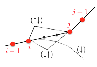
Figure 27: Region between a pair of twin samples, with a twin sample including a corner.

In this case for any index $i\in S_{k}$, we prove $\tilde{z}_{i}={z_{i}^{\star}}=z^{\diamond}_{i}$, i.e., all optimal solutions must reduce to a straight line between the collinear samples. We prove this with the visual support of Fig. 27. Our goal is to show that any $\hat{z}$ that deviates from linearity is not sign consistent (SC), hence cannot be optimal. If a sample $k\in\{i+1,\ldots,j-1\}$ has a curvature different from zero, then, to be sign consistent it cannot change curvature. This case is shown with the label ($\downarrow$) in Fig. 27. Clearly, if $\hat{z}$ cannot change curvature, after deviating from the straight line, it cannot reach the sample $j$, leading to contradiction. Similarly, contradiction occurs when the curvature is different from zero at $i$: a positive curvature at $i$ (case ($\uparrow\downarrow$) in figure), must be compensated by a negative curvature before $j$ for the curve to intersect $j$: this again violates sign consistency; analogous argument holds for a negative curvature at $i$ (case ($\downarrow\uparrow$) in figure). Therefore we proved that in these straight segments it holds $\tilde{z}_{i}={z_{i}^{\star}}=z^{\diamond}_{i}$. If only remains to discuss the case in which $\tilde{z}_{i}\neq z^{\diamond}_{i}$ which occurs whenever consecutive double samples do not include corners. This situation is pictured in Fig. 5(a); in this case $\tilde{z}_{i}\leq z^{\diamond}_{i}$. We only prove that whenever $\tilde{z}_{i}\leq z^{\diamond}_{i}$ then $\tilde{z}_{i}\leq{z_{i}^{\star}}\leq z^{\diamond}_{i}$; the proof for the case $z^{\diamond}_{i}\leq\tilde{z}_{i}$ is practically identical (the corner points downwards). In Fig. 5(a) we show two cases (dashed lines): in case ($\uparrow\downarrow$) we show a profile $\hat{z}$ above $z^{\diamond}$; in ($\downarrow\uparrow$) we show a profile below $\tilde{z}$. One can easily realize than any profile as in case ($\uparrow\downarrow$) has a positive curvature at sample $i$ and a negative curvature at the top corner: this violates sign consistency hence $\hat{z}$ is not in the solution set. A similar argument holds in the case ($\downarrow\uparrow$), which concludes the proof that ${z^{\star}}$ must be “between” $\tilde{z}$ and $z^{\diamond}$.

We conclude the proof by deriving the error bound in eq. (15), repeated below for the reader’s convenience:

$$\|z^{\diamond}-{z^{\star}}\|_{\infty}\leq\max_{i\in{\cal M}}d_{i}\cos(\theta_{i})$$ (60)

where $d_{i}$ is the distance between the sample $i$ and the nearest corner in $z^{\diamond}$, while $\theta_{i}$ is the angle that the line connecting $i$ with the nearest corner forms with the vertical, see Fig. 5(a).The bound relates any solution ${z^{\star}}$ of the $\ell_{1}$-minimization problem ($\text{L1}_{D}$) to the true profile $z^{\diamond}$.

To prove (60), we note that ${z^{\star}}$ can deviate from $z^{\diamond}$ only in the “corner cases” as the one in Fig. 5(a) (proven above in this section). Moreover, we note that the maximum error $|z^{\diamond}_{i}-\tilde{z}_{i}|$ is attained at the corner of $z^{\diamond}$ and is denoted with $\hat{d}$ in the figure. From basic trigonometry we conclude:

$$\hat{d}\leq\max_{k\in\{i,j\}}d_{k}\cos{\theta_{k}}$$ (61)

(in Fig. 5(a) this becomes: $\hat{d}\leq d_{i}\cos(\theta_{i})$), where $d_{k}$ is the distance between sample $k$ and the nearest corner, while $\theta_{k}$ is the angle that the line connecting sample $k$ with the nearest corner forms with the vertical. The bound (60) follows by extending this inequality to all linear segments in $z^{\diamond}$. ∎

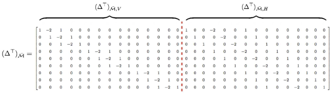
Figure 28: Example of matrix $(\Delta^{\mathsf{T}})_{\overline{{\cal M}}}$ and corresponding column partition $(\Delta^{\mathsf{T}})_{\overline{{\cal M}},V}$, $(\Delta^{\mathsf{T}})_{\overline{{\cal M}},H}$.

Appendix G Proof of Theorem 17

In this section we prove that if a 3D profile $Z$ is feasible for problem ($\text{L1}_{\Delta}$) and it is 3D sign consistent, then it is also a minimizer of ($\text{L1}_{\Delta}$). The proof is similar to the 2D case in Proposition 14, and relies on Corollary 10, which we restate as follows: given a profile $Z\in{{\mathbb{R}}^{r\times c}}$ which is feasible for problem ($\text{L1}_{\Delta}$), $Z$ is in the optimal set of ($\text{L1}_{\Delta}$) if there exists a vector $u\in{{\mathbb{R}}^{2(n-r-c)}}$, with $n=r\times c$, such that

$$(\Delta^{\mathsf{T}})_{\overline{{\cal M}}}\;u={\mathbf{0}}\;\text{ and }\;u_{\cal I}=\text{sign}(\Delta z)_{\cal I}\;\text{ and }\;\|u_{\cal J}\|_{\infty}\leq 1,$$ (62)

where ${\cal M}$ denotes a grid sample set. Let $\overline{{\cal M}}_{i}$ be patches defined in Definition 15. We show that 3D sign consistency of $Z$ with respect to grid samples ${\cal M}$ implies (62). We start by noting that when using grid samples with $K$ patches (see Fig. 6(b)), problem ($\text{L1}_{\Delta}$) separates into $K$ independent optimization subproblems (similarly to the 2D case of eq. (F)). Therefore, without loss of generality in the following we focus on a single patch and we assume that the grid samples include the boundaries of the patch (first and last two rows and columns). With slight abuse of notation we denote this patch with $Z$ and we use $z=\,\text{vec}{\left(Z\right)}$.

Before proving the claim we need some insight on the structure of the matrix $(\Delta^{\mathsf{T}})_{\overline{{\cal M}}}$. This matrix is obtained by deleting rows of $\Delta^{\mathsf{T}}$ indexed by ${\cal M}$. Since we are assuming to sample the boundaries of the patch, the resulting $(\Delta^{\mathsf{T}})_{\overline{{\cal M}}}$ has the structure described in Fig. 28. Now we remain to show that when $Z$ is 3D sign consistent, we can find a vector $u$ that satisfies the three conditions in (62). Towards this goal, we recall that $\Delta$ is obtained by stacking two submatrices that compute the vertical and horizontal differences as in (12). Therefore, we split $\text{sign}(\Delta z)_{\cal I}$ accordingly as:

$$\text{sign}(\Delta z)_{\cal I}=\left[\begin{array}[]{c}\text{sign}(\Delta z)_{{\cal I}_{V}}\\ \text{sign}(\Delta z)_{{\cal I}_{H}}\end{array}\right]$$ (63)

where ${\cal I}_{V}$ includes indices in the support set ${\cal I}$ corresponding to nonzero vertical differences, while ${\cal I}_{H}$ includes indices in ${\cal I}$ corresponding to nonzero horizontal differences.

Now, we note that the row partition of $\Delta$ induces a column partition of $(\Delta^{\mathsf{T}})_{\overline{{\cal M}}}$. We call the corresponding submatrices $(\Delta^{\mathsf{T}})_{\overline{{\cal M}},V}$ and $(\Delta^{\mathsf{T}})_{\overline{{\cal M}},H}$, as shown in Fig. 28. This also partitions the vector $u$ into two subvectors $u_{V}$ and $u_{H}$. Therefore, we rewrite the condition $(\Delta^{\mathsf{T}})_{\overline{{\cal M}}}u={\mathbf{0}}$ as:

$$(\Delta^{\mathsf{T}})_{\overline{{\cal M}},V}\;u_{V}+(\Delta^{\mathsf{T}})_{\overline{{\cal M}},H}\;u_{H}={\mathbf{0}}$$ (64)

Since $Z$ is 3D sign consistent, then $\text{sign}(\Delta z)_{{\cal I}_{V}}$ is either $+{\mathbf{1}}$ or $-{\mathbf{1}}$ and $\text{sign}(\Delta z)_{{\cal I}_{H}}$ is either $+{\mathbf{1}}$ or $-{\mathbf{1}}$. Assume without loss of generality that $\text{sign}(\Delta z)_{{\cal I}_{V}}=+{\mathbf{1}}$ and $\text{sign}(\Delta z)_{{\cal I}_{H}}=-{\mathbf{1}}$. Now if we choose $u_{V}=+{\mathbf{1}}$ and $u_{H}=-{\mathbf{1}}$, it holds that $u_{{\cal I}_{V}}=\text{sign}(\Delta z)_{{\cal I}_{V}}$, $u_{{\cal I}_{H}}=\text{sign}(\Delta z)_{{\cal I}_{H}}$, and $\|u_{\cal J}\|_{\infty}\leq\|u\|_{\infty}\leq 1$, hence the last two conditions in (62) are satisfied. Moreover, since each row of $(\Delta^{\mathsf{T}})_{\overline{{\cal M}},V}$ and $(\Delta^{\mathsf{T}})_{\overline{{\cal M}},H}$ includes only three nonzero entries with values $+1,-2,+1$, it follows that:

$$(\Delta^{\mathsf{T}})_{\overline{{\cal M}},V}\;u_{V}=(\Delta^{\mathsf{T}})_{\overline{{\cal M}},V}\;{\mathbf{1}}={\mathbf{0}}$$

$$(\Delta^{\mathsf{T}})_{\overline{{\cal M}},H}\;u_{H}=-(\Delta^{\mathsf{T}})_{\overline{{\cal M}},H}\;{\mathbf{1}}={\mathbf{0}}$$ (65)

which implies (64), concluding the proof. ∎

Appendix H Proof of Proposition 18

By the assumptions of Proposition 18, $Z^{\diamond}$ is the ground truth generating noiseless measurements (4) and $Z^{\diamond}$ is 3D sign consistent with respect to ${\cal M}$. Then each row of $Z^{\diamond}$, namely $Z^{\diamond}_{i}$, is a sign consistent 2D depth profile and, given the samples, we can build a row-wise envelope for $Z^{\diamond}_{i}$ as prescribed in Theorem 13 (pictorial explanation in Fig. 6(b)). Repeating this procedure for all rows $i$ and calling $\bar{Z}$ and $\underline{Z}$ the point-wise upper bound an lower bound for the envelope of each row, then $Z^{\diamond}$ is within the row-wise envelope, i.e., $\underline{Z}_{i,j}\leq Z^{\diamond}_{i,j}\leq\bar{Z}_{i,j}$ for all $i=1,\ldots,r$ and $j=1,\ldots,c$. Therefore, given an optimal solution ${Z^{\star}}$ of ($\text{L1}_{\Delta}$) it holds that

$$|Z^{\diamond}_{i,j}-Z^{\star}_{i,j}|\leq\max(|\underline{Z}_{i,j}-{Z^{\star}}_{i,j}|,|\bar{Z}_{i,j}-{Z^{\star}}_{i,j}|).$$

which trivially follows from the chain of inequalities $\underline{Z}_{i,j}\leq Z^{\diamond}_{i,j}\leq\bar{Z}_{i,j}$, concluding the proof. ∎

Appendix I Proof of Proposition 19

This appendix proves the necessary and sufficient conditions for an estimate ${z^{\star}}$ to be in the set $\SS$ of optimal solutions of problem ($\text{L1}_{D}^{\varepsilon}$), as stated in Proposition 19. We follow similar arguments as the proof in Appendix D.

We start by rewriting ($\text{L1}_{D}^{\varepsilon}$) as:

$$\min_{z}\|Dz\|_{1}+\chi_{\{z:\|Az-y\|_{\infty}\leq\varepsilon\}}\doteq\min_{z}f(z)$$ (66)

As discussed earlier in Appendix D, a profile ${z^{\star}}$ is optimal for problem ($\text{L1}_{D}^{\varepsilon}$) if the zero vector belongs to the set of subgradients of $f$ at ${z^{\star}}$, i.e., ${\mathbf{0}}\in\partial f({z^{\star}})$. The subdifferential of $\|Dz\|_{1}$ was given in (D). The subdifferential of the indicator function in (66) is given, similarly to (41), as

$$\partial(\chi_{\{z:\|Az-y\|_{\infty}\leq\varepsilon\}})({z^{\star}})=$$

$$\qquad\{g\in{{\mathbb{R}}^{n}}\;{:}\;g^{\mathsf{T}}{z^{\star}}\geq g^{\mathsf{T}}r,\;\forall r\text{ s.t. }\|Ar-y\|_{\infty}\leq\varepsilon\}$$ (67)

Recall that the matrix $A$ restricts a vector $r$ to its entries in the sample set ${\cal M}$, therefore we have

$$\{r:\ \|Ar-y\|_{\infty}\leq\varepsilon\}=\{r:\ \|r_{\cal M}-y\|_{\infty}\leq\varepsilon\}.$$ (68)

Obviously $\|r_{\cal M}-y\|_{\infty}\leq\varepsilon$ implies for all $i\in{\cal M}$ that

$$r_{i}\leq y_{i}+\varepsilon\ \ \text{or}\ \ r_{i}\geq y_{i}-\varepsilon.$$ (69)

We decompose

$$g^{\mathsf{T}}{z^{\star}}\geq g^{\mathsf{T}}r=g^{\mathsf{T}}_{\cal M}r_{\cal M}+g^{\mathsf{T}}_{\overline{{\cal M}}}r_{\overline{{\cal M}}}.$$ (70)

A vector $g$ that satisfies (70), for all $r$ obeying (68), must satisfy $g^{\mathsf{T}}_{\overline{{\cal M}}}={\mathbf{0}}$ since $r_{\overline{{\cal M}}}$ is a free variable. With this at hand, we proceed as

$$g^{\mathsf{T}}{z^{\star}} \geq\max_{\|r_{\cal M}-y\|_{\infty}\leq\varepsilon}g^{\mathsf{T}}_{\cal M}r_{\cal M}=\max_{\|r_{\cal M}-y\|_{\infty}\leq\varepsilon}\sum_{i\in{\cal M}}g_{i}r_{i}$$

$$=\max_{\|r_{\cal M}-y\|_{\infty}\leq\varepsilon}\left(\sum_{\small g_{i}\geq 0,\ i\in{\cal M}}|g_{i}|r_{i}-\sum_{\small g_{i}<0,\ i\in{\cal M}}|g_{i}|r_{i}\right)$$

$$=\sum_{\small g_{i}\geq 0,\ i\in{\cal M}}|g_{i}|(y_{i}+\varepsilon)-\sum_{\small g_{i}<0,\ i\in{\cal M}}|g_{i}|(y_{i}-\varepsilon)$$

$$=\sum_{\small g_{i}\geq 0,\ i\in{\cal M}}|g_{i}|y_{i}-\sum_{\small g_{i}<0,\ i\in{\cal M}}|g_{i}|y_{i}+\varepsilon\sum_{i\in{\cal M}}|g_{i}|$$

$$=g^{\mathsf{T}}_{\cal M}y+\varepsilon\|g_{\cal M}\|_{1}.$$

Rearranging terms yields

$$\|g_{\cal M}\|_{1}\leq\frac{g^{\mathsf{T}}_{\cal M}(z_{\cal M}^{\star}-y)}{\varepsilon}.$$ (71)

We can then write the solution set as

$$\SS=\{{z^{\star}} : \exists u\in{{\mathbb{R}}^{n-2}},g\in{{\mathbb{R}}^{n}},\text{ such that }$$

$$D^{\mathsf{T}}u+g={\mathbf{0}},$$

$$u_{\cal I}=\text{sign}(D{z^{\star}})_{\cal I},\;\;\|u_{\cal J}\|_{\infty}\leq 1,$$

$$\|g_{\cal M}\|_{1}\leq\frac{g^{\mathsf{T}}_{\cal M}(z_{\cal M}^{\star}-y)}{\varepsilon},$$

$$g^{\mathsf{T}}_{\overline{{\cal M}}}={\mathbf{0}}\}.$$ (72)

The conditions $D^{\mathsf{T}}u+g={\mathbf{0}}$ and $g^{\mathsf{T}}_{\overline{{\cal M}}}={\mathbf{0}}$ can be cast as $(D^{\mathsf{T}})_{\overline{{\cal M}}}\;u={\mathbf{0}}$ and $g_{\cal M}=-(D^{\mathsf{T}})_{\cal M}\;u$. Then inequality in (71) must be an equality since $|z_{\cal M}^{\star}-y|\leq\varepsilon$ (hence $\frac{\|z_{\cal M}^{\star}-y\|_{\infty}}{\varepsilon}\leq 1$) and $\|g_{\cal M}\|_{1}\doteq\max_{v:\|v\|_{\infty}\leq 1}g^{\mathsf{T}}_{\cal M}v$ by definition of the $\ell_{1}$-norm; moreover if $|z_{i}^{\star}-y_{i}|=\varepsilon$ for some $i\in{\cal M}$ it must hold that

$$\text{sign}((D^{\mathsf{T}})_{i}\;u)=(z_{i}^{\star}-y_{i})/\varepsilon.$$ (73)

Here we used the assumption that $\varepsilon>0$. Denote the set of such $i\in{\cal M}$ as the active set ${\cal A}$ as in (17). For $i\in{\cal M}\setminus{\cal A}$, it holds that $(D^{\mathsf{T}})_{i}\;u={\mathbf{0}}$. Splitting ${\cal A}$ into two subsets as in (19) and using (73) yields the conditions (20) of Proposition 19. ∎

Appendix J Proof of Proposition 23

To prove the claim of Proposition 23, we show that any 2D sign consistent profile is bounded above by $\bar{z}$ and below by $\underline{z}$ as defined in Definition 22. We restrict the proof to demonstrate the validity of the upper bound, since the argument for the lower bound follows similarly. To this end, we focus on line segments (1), (3) and (5) that determine $\bar{z}$. Fig. 29(a)-(d) illustrate 4 possible orientations of these line segments and the resulting upper bounds (in solid blue line).

Let us start with the case of Fig. 29(a). We use a contradiction argument similarly to the proof of Proposition 14. We show that a profile which is not upper bounded by the solid blue line, that is $\max\{(1),(3)\}$ in this case, has to be sign inconsistent (Definition 11). Indeed such a profile needs to have a nonzero curvature at sample either $i+1$ or $j$ since the line segments (1) and (3) represent the extreme slopes that a profile can have with zero curvature at the end points. Assume without loss of generality, a profile (dashed black line in Fig. 29(a)) that has positive curvature at $i+1$ (label ($\downarrow\uparrow$) in figure) and violates the upper bound. It is clear that this profile cannot reach the $\epsilon$-interval (red bar in figure) at sample $j$ without having a negative curvature between $i+1$ and $j$; this violates sign consistency (case (i) in Definition 11), leading to contradiction.

Next we prove the claim for Fig. 29(b). In this case the upper bound $\bar{z}$ is given by the line segment (5). Any profile that is not upper-bounded by (5) needs to have a positive curvature ($\downarrow\uparrow$) between $i+1$ and $j$. It is obvious that such a profile also needs to have a negative curvature at some other sample $k\in(i+1,j)$ to reach the $\epsilon$-interval at sample $j$, which leads to contradiction.

Finally, observe that Fig. 29(c) and Fig. 29(d) are exactly symmetrical cases with different orientations for line segments (1) and (3). Therefore we consider only Fig. 29(c) here. Similarly to before, a profile (dashed black line in figure) that is not upper bounded by (5) needs to have a positive curvature between $i+1$ and $j$. However in order to reach the $\epsilon$-bar at sample $i+1$, this profile must have a negative curvature at some other sample $k\in(i+1,j)$, which contradicts sign consistency.

We proved the claim of the proposition for all possible cases in Fig. 29 which ends our proof. ∎

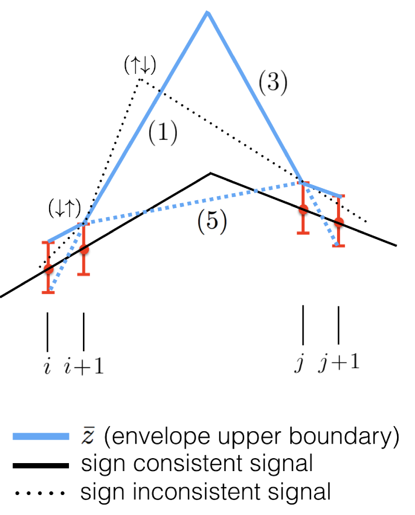
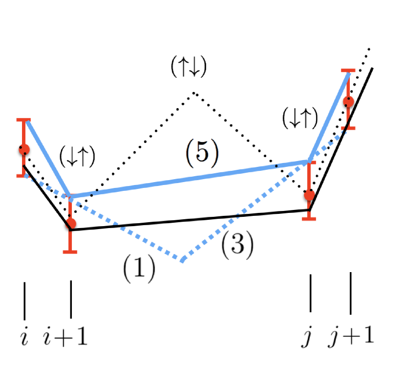
(a) (b)

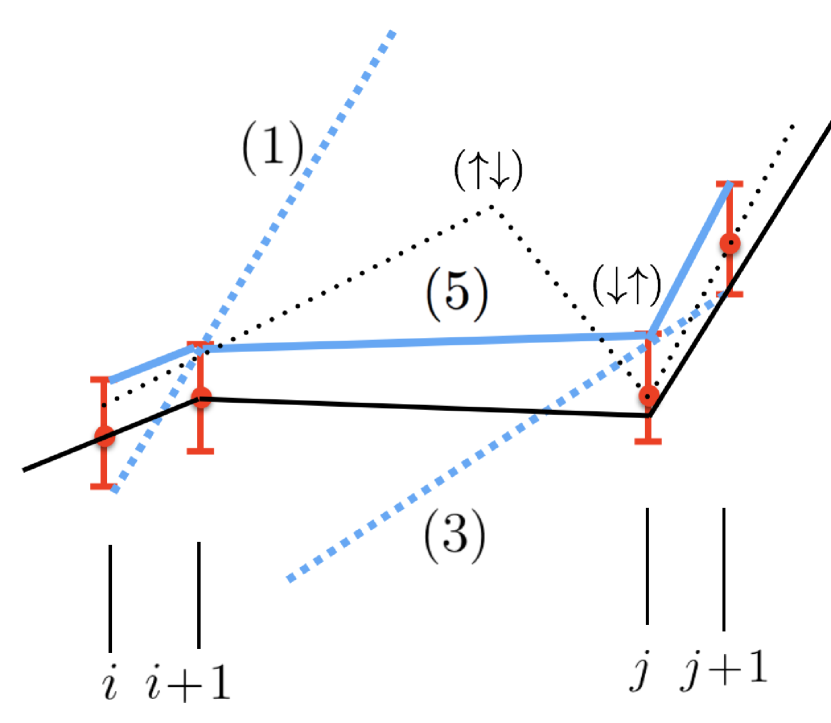
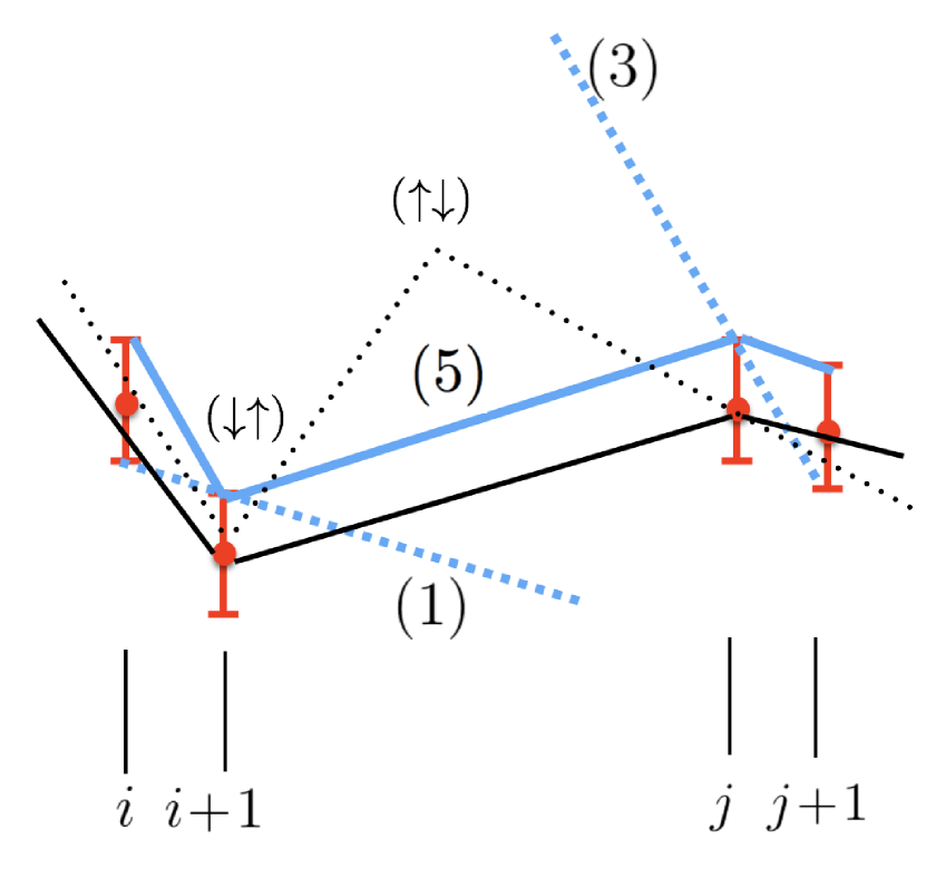
(c) (d)

Figure 29: Illustration of the upper bound $\bar{z}$ of 2D sign consistent $\epsilon$-envelope for all possible orientations of the line segments (1), (3) and (5) defined in Definition 22.

Appendix K Proof of Proposition 24

From Theorem 21 we learn that any optimal solution ${z^{\star}}$ must be 2D sign consistent, implying that it lies within the 2D sign consistent $\epsilon$-envelope. By the assumptions of Proposition 24 that we sample the boundary of $z^{\diamond}$ and the sample set includes a twin sample in each linear segment in $z^{\diamond}$, it follows that the ground truth profile $z^{\diamond}$ is also sign consistent (see discussion in Appendix F), hence belongs to the 2D sign consistent $\epsilon$-envelope as a result of Proposition 23.

Since both ${z^{\star}}$ and $z^{\diamond}$ lie inside the same 2D envelope, the difference between ${z_{k}^{\star}}$ and $z^{\diamond}_{k}$ for arbitrary $k\in(i+1,j)$ is bounded by the difference between the top and the bottom of the envelope, $\bar{z}_{k}-\underline{z}_{k}$. ∎

Appendix L Proof of Corollary 26

In the proof of Proposition 14 (Appendix F) we have seen that the objective of ($\text{L1}_{D}$) is separable as in (F), where $S_{k}$ includes all indices falling in the region between two consecutive twin samples (e.g., if the twin samples are $(i-1,i)$ and $(j,j+1)$, then $S_{k}=\{i-1,i,i+1,\ldots,j-1,j,j+1\}$). This allows us to study the performance of Algorithm 1 independently for each region $S_{k}$. As a result of Proposition 14, line 1 in Algorithm 1 produces a solution ${z^{\star}}$ between $\tilde{z}$ and $z^{\diamond}$. Assume without loss of generality that ${z^{\star}}$ is concave in the region $S_{k}$, e.g., the leftmost corner of Fig. 2(b), which yields $s_{k}=-1$ in line 1. Then $\tilde{z}_{i}\leq{z_{i}^{\star}}\leq z^{\diamond}_{i}$ for all $i\in S_{k}$ which implies

$$\sum_{i\in S_{k}}{z_{i}^{\star}}\leq\sum_{i\in S_{k}}z^{\diamond}_{i}$$ (74)

Now we note that maximizing $\sum_{i\in S_{k}}z_{i}$ is the same as minimizing $-\sum_{i\in S_{k}}z_{i}$. Therefore, when $s_{k}=-1$, line 1 maximizes the objective $\sum_{i\in S_{k}}z_{i}$ subject to $z\in\SS$ where $\SS$ is the optimal set of ($\text{L1}_{D}$). Since (74) holds for all $z\in\SS$, and since $z^{\diamond}\in\SS$, Algorithm 1 returns $z^{\diamond}$. ∎

Appendix M Computation for NESTA

In this appendix we provide some technical details as well as closed-form expressions related to Algorithm 2.

The function $f_{\mu}$ in (28) is shown to be differentiable by Nesterov [71] and has gradient

$$\nabla f_{\mu}(z)=D^{\mathsf{T}}u^{\star}(z)$$ (75)

where $u^{\star}(z)$ is the optimal solution of the maximization in (28) and, for any given $z$, can be computed as

$$u^{\star}(z)=\left\{\begin{array}[]{ll}\mu^{-1}(Dz)_{i},&\text{if }|(Dz)_{i}|<\mu\\ \text{sign}(Dz)_{i},&\text{otherwise}.\end{array}\right.$$ (78)

The gradient $\nabla f_{\mu}(z)$ is said to be Lipschitz with Lipschitz constant $L_{\mu}$ if it obeys

$$\|\nabla f_{\mu}(x)-\nabla f_{\mu}(z)\|_{2}\leq L_{\mu}\|x-z\|_{2}.$$

The constant $L_{\mu}$, used in Algorithm 2, is shown to be $L_{\mu}=\frac{\|D\|^{2}}{\mu}$ in [18, eq (3.4)], where $\|\cdot\|$ denotes the spectral norm of a matrix.

Next we provide closed-form solutions for the optimization problems in lines 2-2 of Algorithm 2. We start with $\bar{q}$, which is the solution of the optimization problem in line 2. Eliminating constant terms in the objective in line 2 and completing the squares yields:

$$\bar{q}= \mathrm{argmin}_{z\in{\cal Q}}\;\frac{L_{\mu}}{2}\|z-z^{(k)}\|_{2}^{2}+{\langle}g,z{\rangle}$$

$$= \mathrm{argmin}_{z\in{\cal Q}}\|z-(z^{(k)}-L_{\mu}^{-1}g)\|_{2}^{2}$$ (79)

where $g\doteq\nabla f_{\mu}(z^{(k)})$ and ${\cal Q}\doteq\{z:\|Az-y\|_{\infty}\leq\varepsilon\}$. For simplicity we introduce the vector $\hat{z}^{(k)}\doteq z^{(k)}-L_{\mu}^{-1}g$, and recall that the sampling matrix $A$ restricts a vector to its entries at indices in ${\cal M}$, hence ${\cal Q}=\{z:\|z_{\cal M}-y\|_{\infty}\leq\varepsilon\}$. We then notice that the objective in (M) separates as:

$$\bar{q}=\displaystyle\mathrm{argmin}_{z_{\cal M}\in{\cal Q}}\|[z-\hat{z}^{(k)}]_{\cal M}\|_{2}^{2}+\|[z-\hat{z}^{(k)}]_{\overline{{\cal M}}}\|_{2}^{2}$$ (80)

which further separates into two independent optimization problems involving subvectors of $\bar{q}$:

$$\bar{q}_{\cal M}=\mathrm{argmin}_{z_{\cal M}\in{\cal Q}}\|[z-\hat{z}^{(k)}]_{\cal M}\|_{2}^{2}$$ (81)

$$\bar{q}_{\overline{{\cal M}}}=\mathrm{argmin}_{z_{\overline{{\cal M}}}}\|[z-\hat{z}^{(k)}]_{\overline{{\cal M}}}\|_{2}^{2}$$ (82)

Problem (82) is an unconstrained minimization, since ${\cal Q}$ only constraints $z_{\cal M}$. By inspection, problem (82) admits the trivial solution $\bar{q}_{\overline{{\cal M}}}=\hat{z}^{(k)}_{\overline{{\cal M}}}$. It remains to solve (81):

$$\bar{q}_{\cal M}=\mathrm{argmin}_{\zeta}\|\zeta-\hat{z}^{(k)}_{\cal M}\|_{2}^{2}\quad\text{ subject to }\|\zeta-y\|_{\infty}\leq\varepsilon$$ (83)

where we “renamed” the optimization variable to $\zeta$ to simplify notation. Problem (83) is nothing but the Euclidean projection of the vector $\hat{z}^{(k)}_{\cal M}$ onto the $\ell_{\infty}$-ball with radius $\varepsilon$ centered at $y$. This projection can be explicitly calculated as:

$$\bar{q}_{i}=\min\{\max\{\hat{z}^{(k)}_{i},y_{i}-\varepsilon\},y_{i}+\varepsilon\},\ \ \forall i\in{\cal M}.$$

which completes the derivation of the closed-form solution for $\bar{q}$. The reader may notice that the optimization problem in line 2 of Algorithm 2, whose solution is $\bar{w}$, is identical to the one in (M), after replacing $g=\sum_{i=0}^{k}\alpha_{i}\nabla f_{\mu}(z^{(i)})$ and using $z^{(0)}$ instead of $z^{(k)}$. For this reason the closed-form solution $\bar{w}$ can be derived in full similarity with the one of $\bar{q}$, and can be explicitly written as:

$$\bar{w}_{\overline{{\cal M}}} = \breve{z}^{(k)}_{\overline{{\cal M}}}$$

$$\bar{w}_{i} = \min\{\max\{\breve{z}^{(k)}_{i},y_{i}-\varepsilon\},y_{i}+\varepsilon\},\ \ \forall i\in{\cal M},$$

where $\breve{z}^{(k)}\doteq z^{(0)}-L_{\mu}^{-1}\sum_{i=0}^{k}\alpha_{i}\nabla f_{\mu}(z^{(i)})$.

Appendix N Extra Visualizations: Gazebo Depth Images

			Reconstructed profiles
	Depth profile	samples	naive	L1	L1diag
uniform
	3D depth	2% samples
RBG edges
	RGB image	RGB edges

Figure 30: Gazebo: 3 examples of reconstructed depth profiles using the proposed approaches (L1, L1diag) and a naive linear interpolation (naive). For each example we show the reconstruction from 2% uniformly drawn depth measurements. We also show the reconstruction for the case in which we can access the depth corresponding to (appearance) edges in the RGB images.

Appendix O Extra Visualizations: ZED Depth Images

Figure 31: ZED: 6 examples of reconstructed depth profiles using the proposed approaches (L1, L1diag) and a naive linear interpolation (naive). For each example we show the reconstruction from 2% uniformly drawn depth measurements. We also show the reconstruction for the case in which we can access the depth corresponding to (appearance) edges in the RGB images.

References

- [1] R. Wood, “RoboBees project,” Harvard University, 2015. [Online]. Available: http://robobees.seas.harvard.edu/
- [2] “Meet piccolissimo: The world’s smallest self-powered controllable flying vehicle,” University of Pennsylvania, 2016.
- [3] C. De Wagter, S. Tijmons, B. D. Remes, and G. C. de Croon, “Autonomous flight of a 20-gram flapping wing mav with a 4-gram onboard stereo vision system,” in 2014 IEEE International Conference on Robotics and Automation (ICRA). IEEE, 2014, pp. 4982–4987.
- [4] G. De Croon, C. De Wagter, B. Remes, and R. Ruijsink, “Sub-sampling: real-time vision for micro air vehicles,” Robotics and Autonomous Systems, vol. 60, no. 2, pp. 167–181, 2012.
- [5] “Pd-100 black hornet prs,” proxdynamics, 2016. [Online]. Available: http://www.proxdynamics.com/products/pd-100-black-hornet-prs
- [6] D. W. Haldane, M. Plecnik, J. K. Yim, and R. S. Fearing, “Robotic vertical jumping agility via series-elastic power modulation,” Science Robotics, 2016.
- [7] R. Newcombe, S. Lovegrove, and A. Davison, “DTAM: Dense tracking and mapping in real-time,” in Intl. Conf. on Computer Vision (ICCV), Barcelona, Spain, Nov 2011, pp. 2320–2327.
- [8] R. Mur-Artal, J. Montiel, and J. Tardós, “ORB-SLAM: A versatile and accurate monocular SLAM system,” IEEE Trans. Robotics, vol. 31, no. 5, pp. 1147–1163, 2015.
- [9] T. Whelan, S. Leutenegger, R. Salas-Moreno, B. Glocker, and A. Davison, “ElasticFusion: Dense SLAM without a pose graph,” in Robotics: Science and Systems (RSS), 2015.
- [10] S. Suri, E. Vicari, and P.Widmayer, “Simple robots with minimal sensing: From local visibility to global geometry,” Intl. J. of Robotics Research, vol. 27, 2008.
- [11] J. Derenick, A. Speranzon, and R. Ghrist, “Homological sensing for mobile robot localization,” in IEEE Intl. Conf. on Robotics and Automation (ICRA), 2013, pp. 572–579.
- [12] B. Tovar, L. Freda, and S. M. LaValle, “Learning combinatorial map information from permutations of landmarks,” Intl. J. of Robotics Research, vol. 30, no. 9, pp. 1143–1156, 2011.
- [13] B. Tovar, F. Cohen, L. Bobadilla, J. Czarnowski, and S. M. LaValle, “Combinatorial filters: Sensor beams, obstacles, and possible paths,” ACM Transactions on Sensor Networks, vol. 10, no. 3, 2014.
- [14] X. Chen, M. Zhao, L. Xiang, F. Sugai, H. Yaguchi, K. Okada, and M. Inaba, “Development of a low-cost ultra-tiny line laser range sensor,” in Intelligent Robots and Systems (IROS), 2016 IEEE/RSJ International Conference on. IEEE, 2016, pp. 111–116.
- [15] C. Poulton and M. Watts, “Mit and darpa pack lidar sensor onto single chip,” IEEE Spectrum, 2016. [Online]. Available: http://spectrum.ieee.org/tech-talk/semiconductors/optoelectronics/mit-lidar-on-a-chip
- [16] TeraRanger, “Teraranger one,” http://www.teraranger.com/, 2016. [Online]. Available: http://www.teraranger.com/products/teraranger-one/
- [17] LeddarVu, “Leddarvu solid-state lidar platform,” http://leddartech.com/, 2016. [Online]. Available: http://leddartech.com/modules/leddarvu/
- [18] S. Becker, J. Bobin, and E. J. Candès, “Nesta: A fast and accurate first-order method for sparse recovery,” SIAM Journal on Imaging Sciences, vol. 4, no. 1, pp. 1–39, 2011.
- [19] F. Ma, L. Carlone, U. Ayaz, and S. Karaman, “Sparse sensing for resource-constrained depth reconstruction,” in Intl. Conf. on Intelligent Robots and Systems, submitted, 2016.
- [20] K. Goldberg, “Orienting polygonal parts without sensors,” Algorithmica, vol. 10, pp. 201–225, 1993.
- [21] P. Boning and S. Dubowsky, “A study of minimal sensor topologies for space robots,” Advances in Robot Kinematics, Springer, pp. 413–422, 2006.
- [22] J. M. O’Kane and S. M. LaValle, “On comparing the power of mobile robots,” in Robotics: Science and Systems (RSS), 2006.
- [23] N. Shrivastava, R. Madhow, and S. Suri, “Target tracking with binary proximity sensors: fundamental limits, minimal descriptions, and algorithms,” in Proc. of the 4th Intl. Conf. on Embedded Networked Sensor Systems, 2006, pp. 251–264.
- [24] B. Tovar, L. Freda, and S. LaValle, “Mapping and navigation from permutations of landmarks,” AMS Contemporary Mathematics, vol. 438, pp. 33–45, 2007.
- [25] D. Marinakis, P. Giguere, and G. Dudek, “Learning network topology from simple sensor data,” in Prof. Canadian Conference on Artificial Intelligence, 2002.
- [26] D. Marinakis and G. Dudek, “Occam’s razor applied to network topology inference,” IEEE Trans. Robotics, vol. 24, no. 2, pp. 293–306, April 2008.
- [27] J. M. O’Kane and S. M. LaValle, “Localization with limited sensing,” IEEE Trans. Robotics, vol. 23, pp. 704–716, 2007.
- [28] L. Erickson, J. Knuth, J. O’Kane, and S. LaValle, “Probabilistic localization with a blind robot,” in IEEE Intl. Conf. on Robotics and Automation (ICRA), 2008, pp. 1821–1827.
- [29] B. Tovar and S. M. LaValle, “Searching and mapping among indistinguishable convex obstacles,” in IEEE Intl. Conf. on Robotics and Automation (ICRA), 2010.
- [30] B. Tovar, F. Cohen, and S. M. LaValle, “Sensor beams, obstacles, and possible paths,” in Intl. Workshop on the Algorithmic Foundations of Robotics, 2008.
- [31] M. Milford, “Vision-based place recognition: how low can you go?” Intl. J. of Robotics Research, vol. 32, pp. 766–789, 2013.
- [32] T. Kanade, “Recovery of the 3-dimensional shape of an object from a single view,” Artificial Intelligence, vol. 17, 1981.
- [33] W. Hong, A. Yang, K. Huang, and Y. Ma, “On symmetry and multiple view geometry: Structure, pose and calibration from a single image,” Intl. J. of Computer Vision, no. 3, 2004.
- [34] O. D. Faugeras and F. Lustman, “Motion and structure from motion in a piecewise planar environment,” International Journal of Pattern Recognition and Artificial Intelligence, vol. 2, no. 03, pp. 485–508, 1988.
- [35] S. Pillai, S. Ramalingam, and J. Leonard, “High-performance and tunable stereo reconstruction,” in IEEE Intl. Conf. on Robotics and Automation (ICRA), 2016.
- [36] A. Dame, V. A. Prisacariu, C. Y. Ren, and I. Reid, “Dense reconstruction using 3d object shape priors,” in Proceedings of the IEEE Conference on Computer Vision and Pattern Recognition, 2013, pp. 1288–1295.
- [37] V. Estellers, S. Soatto, and X. Bresson, “Adaptive regularization with the structure tensor,” IEEE Transactions on Image Processing, vol. 24, no. 6, pp. 1777–1790, 2015.
- [38] J. Lu and D. Forsyth, “Sparse depth super resolution,” in 2015 IEEE Conference on Computer Vision and Pattern Recognition (CVPR). IEEE, 2015, pp. 2245–2253.
- [39] P. Piniés, L. Paz, and P. Newman, “Too much TV is bad: dense reconstruction from sparse laser with non-convex regularisation,” in IEEE Intl. Conf. on Robotics and Automation (ICRA), Seattle, WA, USA, May 2015.
- [40] E. Nelson and N. Michael, “Information-theoretic occupancy grid compression for high-speed information-based exploration,” in IEEE/RSJ Intl. Conf. on Intelligent Robots and Systems (IROS), 2015, pp. 4976–4982.
- [41] F. Ramos and L. Ott, “Hilbert maps: scalable continuous occupacy mapping with stochastic gradient descent,” in Robotics: Science and Systems (RSS), 2015.
- [42] S. T. O’Callaghan and F. T. Ramos, “Gaussian process occupancy maps for dynamic environments,” in Experimental Robotics. Springer, 2016, pp. 791–805.
- [43] J. Im, A. Leonessa, and A. Kurdila, “A real-time data compression and occupancy grid map generation for ground-based 3d lidar data using wavelets,” in Proceedings of the ASME 2010 Dynamic Systems and Control Conference, 2010.
- [44] M. Ruhnke, L. Bo, D. Fox, and W. Burgard, “Compact rgbd surface models based on sparse coding,” in Nat. Conf. on Artificial Intelligence (AAAI), 2013.
- [45] ——, “Hierarchical sparse coded surface models,” in IEEE Intl. Conf. on Robotics and Automation (ICRA), 2014, pp. 6238–6243.
- [46] B. Mu, L. Paull, A.-A. Agha-Mohammadi, J. J. Leonard, and J. P. How, “Two-stage focused inference for resource-constrained minimal collision navigation,” IEEE Transactions on Robotics, vol. 33, no. 1, pp. 124–140, 2017.
- [47] B. Mu, A.-a. Agha-mohammadi, L. Paull, M. Graham, J. How, and J. Leonard, “Two-stage focused inference for resource-constrained collision-free navigation,” 2015.
- [48] E. Candès and T. Tao, “Near optimal signal recovery from random projections: Universal encoding strategies?” IEEE Trans. Inform. Theory, vol. 52, no. 12, pp. 5406–5425, 2006.
- [49] D. Donoho, “Compressed sensing,” IEEE Trans. Inform. Theory, vol. 52, no. 4, pp. 1289–1306, 2006.
- [50] E. Candès and M. Wakin, “An introduction to compressive sampling,” IEEE Signal Processing Magazine, vol. 25, no. 2, pp. 21–30, 2008.
- [51] S. Foucart and H. Rauhut, A Mathematical Introduction to Compressive Sensing. Boston: Birkhäuser, 2013.
- [52] X. Liang, X. Ren, Z. Zhang, and Y. Ma, “Repairing sparse low-rank texture,” in European Conf. on Computer Vision (ECCV), 2012, pp. 482–495.
- [53] D. Needell and R. Ward, “Stable image reconstruction using total variation minimization.” SIAM J. Imaging Sci., vol. 6, no. 2, pp. 1035–1058, 2013.
- [54] B. Usevitch, “A tutorial on modern lossy wavelet image compression: Foundations of jpeg 2000,” Signal Processing Magazine, vol. 18, no. 5, pp. 22–35, 2001.
- [55] D. Reddy, A. C. Sankaranarayanan, V. Cevher, and R. Chellappa, “Compressed sensing for multi-view tracking and 3-D voxel reconstruction,” in Intl. Conf. on Image Processing (ICIP), 2008, pp. 221–224.
- [56] Z. Du and G. Geng, “3-D geometric signal compression method based on compressed sensing,” in Image Analysis and Signal Processing, 2011, pp. 62–66.
- [57] B. Hollis, S. Patterson, and J. Trinkle, “Compressed sensing for scalable robotic tactile skins,” arXiv preprint arXiv:1705.05247, 2017.
- [58] S. Vaiter, G. Peyré, C. Dossal, and J. Fadili, “Robust sparse analysis regularization,” IEEE Transactions on information theory, vol. 59, no. 4, pp. 2001–2016, 2013.
- [59] B. Recht, M. Fazel, and P. A. Parrilo, “Guaranteed minimum-rank solutions of linear matrix equations via nuclear norm minimization,” SIAM Rev., vol. 52, no. 3, pp. 471–501, Aug. 2010. [Online]. Available: http://dx.doi.org/10.1137/070697835
- [60] D. B. Phillips, M.-J. Sun, J. M. Taylor, M. P. Edgar, S. M. Barnett, G. G. Gibson, and M. J. Padgett, “Adaptive foveated single-pixel imaging with dynamic super-sampling,” arXiv preprint arXiv:1607.08236, 2016.
- [61] M. F. Duarte, M. A. Davenport, D. Takhar, J. N. Laska, T. Sun, K. E. Kelly, R. G. Baraniuk et al., “Single-pixel imaging via compressive sampling,” IEEE Signal Processing Magazine, vol. 25, no. 2, p. 83, 2008.
- [62] B. Sun, M. P. Edgar, R. Bowman, L. E. Vittert, S. Welsh, A. Bowman, and M. Padgett, “3d computational imaging with single-pixel detectors,” Science, vol. 340, no. 6134, pp. 844–847, 2013.
- [63] S. Nam, M. Davies, M. Elad, and R. Gribonval, “The cosparse analysis model and algorithms,” Applied and Computational Harmonic Analysis, vol. 34, no. 1, pp. 30–56, 2013.
- [64] M. Kabanava and H. Rauhut, “Cosparsity in compressed sensing,” in Compressed Sensing and Its Applications, H. Boche, R. Calderbank, G. Kutyniok, and J. Vybiral, Eds. Springer, 2015, pp. 315–339.
- [65] L. I. Rudin, S. Osher, and E. Fatemi, “Nonlinear total variation based noise removal algorithms,” Phys. D, vol. 60, no. 1-4, pp. 259–268, Nov. 1992. [Online]. Available: http://dx.doi.org/10.1016/0167-2789(92)90242-F
- [66] S. Hawe, M. Kleinsteuber, and K. Diepold, “Dense disparity maps from sparse disparity measurements,” in Computer Vision (ICCV), 2011 IEEE International Conference on. IEEE, 2011, pp. 2126–2133.
- [67] L.-K. Liu, S. H. Chan, and T. Q. Nguyen, “Depth reconstruction from sparse samples: Representation, algorithm, and sampling,” IEEE Transactions on Image Processing, vol. 24, no. 6, pp. 1983–1996, 2015.
- [68] E. Candes and T. Tao, “The dantzig selector: Statistical estimation when p is much larger than n,” The Annals of Statistics, pp. 2313–2351, 2007.
- [69] M. Grant and S. Boyd, “CVX: Matlab software for disciplined convex programming, version 2.1,” http://cvxr.com/cvx, Mar. 2014.
- [70] ——, “Graph implementations for nonsmooth convex programs,” in Recent Advances in Learning and Control, ser. Lecture Notes in Control and Information Sciences, V. Blondel, S. Boyd, and H. Kimura, Eds. Springer-Verlag Limited, 2008, pp. 95–110, http://stanford.edu/~boyd/graph_dcp.html.
- [71] Y. Nesterov, “Smooth minimization of non-smooth functions,” Math. Program., vol. 103, no. 1, pp. 127–152, May 2005. [Online]. Available: http://dx.doi.org/10.1007/s10107-004-0552-5
- [72] ——, “A method for unconstrained convex minimization problem with the rate of convergence o (1/k2),” in Doklady an SSSR, vol. 269, no. 3, 1983, pp. 543–547.
- [73] B. Gerkey, R. T. Vaughan, and A. Howard, “The player/stage project: Tools for multi-robot and distributed sensor systems,” in Proceedings of the 11th international conference on advanced robotics, vol. 1, 2003, pp. 317–323.
- [74] G. Grisetti, C. Stachniss, and W. Burgard, “Improved techniques for grid mapping with Rao-Blackwellized particle filters,” IEEE Trans. Robotics, vol. 23, no. 1, pp. 34–46, 2007.
- [75] N. Koenig and A. Howard, “Design and use paradigms for gazebo, an open-source multi-robot simulator,” in Intelligent Robots and Systems, 2004.(IROS 2004). Proceedings. 2004 IEEE/RSJ International Conference on, vol. 3. IEEE, 2004, pp. 2149–2154.
- [76] D. Scharstein and C. Pal, “Learning conditional random fields for stereo,” in Computer Vision and Pattern Recognition, 2007. CVPR’07. IEEE Conference on. IEEE, 2007, pp. 1–8.
- [77] H. Hirschmuller and D. Scharstein, “Evaluation of cost functions for stereo matching,” in Computer Vision and Pattern Recognition, 2007. CVPR’07. IEEE Conference on. IEEE, 2007, pp. 1–8.
- [78] J. Canny, “A computational approach to edge detection,” IEEE Transactions on Pattern Analysis and Machine Intelligence, 1986.
- [79] C. da Fonseca and J. Petronilho, “Explicit inverses of some tridiagonal matrices,” Linear Algebra and its Applications, vol. 325, pp. 7–12, 2001.
- [80] D. Bertsekas and J. Tsitsiklis, Parallel and Distributed Computation: Numerical Methods. Englewood Cliffs, NJ: Prentice-Hall, 1989.
- [81] S. Boyd and L. Vandenberghe, “Subgradients,” 2006, notes for EE364b.
- [82] D. Bertsekas, A. Nedic, and A. Ozdaglar, Convex Analysis and Optimization. Athena Scientific, 2003.