Resonances for obstacles in hyperbolic space

Abstract.

We consider scattering by star-shaped obstacles in hyperbolic space and show that resonances satisfy a universal bound $\operatorname{Im}\lambda\leq-\frac{1}{2}$ which is optimal in dimension $2$. In odd dimensions we also show that $\operatorname{Im}\lambda\leq-\frac{\mu}{\rho}$ for a universal constant $\mu$, where $\rho$ is the radius of a ball containing the obstacle; this gives an improvement for small obstacles. In dimensions $3$ and higher the proofs follow the classical vector field approach of Morawetz, while in dimension $2$ we obtain our bound by working with spaces coming from general relativity. We also show that in odd dimensions resonances of small obstacles are close, in a suitable sense, to Euclidean resonances.

1. Introduction

For $\kappa>0$ we define hyperbolic $n$-space with constant curvature $-\kappa^{2}$ as

$$({\mathbb{H}}^{n}_{\kappa},g_{\kappa})=({\mathbb{R}}^{n},dr^{2}+s_{\kappa}^{2}h),$$ (1.1)

where $(r,\omega)$ are polar coordinates on ${\mathbb{R}}^{n}$, $h=h(\omega,d\omega)$ is the round metric on $\mathbb{S}^{n-1}$, and $s_{\kappa}(r)=\kappa^{-1}\sinh(\kappa r)$. We include Euclidean space as the case of $\kappa=0$, $s_{0}(r)=r$.

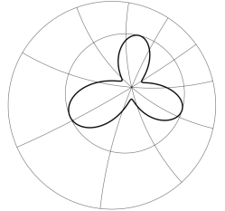
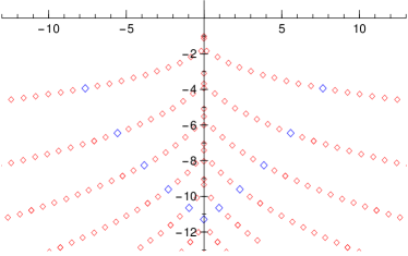
Figure 1. Left: a star-shaped obstacle in the Poincaré disc with resonances satisfying a universal bound $\operatorname{Im}\lambda\leq-\frac{1}{2}$. Right: resonances of a disk with radius $R=1$ in ${\mathbb{H}}^{2}$. Highlighted are resonances corresponding to $\ell=12$ (in the notation of §2).

Suppose that $\mathcal{O}\subset{\mathbb{R}}^{n}\simeq{\mathbb{H}}_{\kappa}^{n}$ is a bounded open set with smooth boundary, and denote by

$$P_{\kappa}:=-\Delta_{g_{\kappa}}-\left(\textstyle\frac{n-1}{2}\right)^{2}\kappa^{2}$$ (1.2)

the self-adjoint operator on $L^{2}(\mathbb{H}_{\kappa}^{n}\setminus\mathcal{O},d\operatorname{vol}_{g_{\kappa}})$ with domain

$$\mathcal{D}(P_{\kappa}):=H^{2}(\mathbb{H}_{\kappa}^{n}\setminus\mathcal{O})\cap H_{0}^{1}(\mathbb{H}_{\kappa}^{n}\setminus\mathcal{O}).$$

The resolvent of $P_{\kappa}$, $\kappa>0$,

$$R_{\kappa}(\lambda):=(P_{\kappa}-\lambda^{2})^{-1}\colon L^{2}({\mathbb{H}}^{n}_{\kappa}\setminus{\mathcal{O}})\to L^{2}({\mathbb{H}}^{n}_{\kappa}\setminus{\mathcal{O}}),\ \ \ \operatorname{Im}\lambda>0,$$ (1.3)

continues meromorphically to a family of operators defined on ${\mathbb{C}}$:

$$R_{\kappa}(\lambda)\colon L^{2}_{{\mathrm{comp}}}({\mathbb{H}}^{n}_{\kappa}\setminus{\mathcal{O}})\to L^{2}_{{\mathrm{loc}}}({\mathbb{H}}^{n}_{\kappa}\setminus{\mathcal{O}}).$$

For $\kappa=0$, the same result is true when $n$ is odd; in even dimensions the continuation takes place on the logarithmic plane.

We denote the set of poles of $R_{\kappa}(\lambda)$ (included according to their multiplicities (3.2)) by $\operatorname{Res}(\mathcal{O},\kappa)$. The elements of $\operatorname{Res}(\mathcal{O},\kappa)$ are called scattering resonances and they determine decay and oscillations of reflected waves outside of $\mathcal{O}$ – see [Zw17] for a recent survey and references. In the odd-dimensional Euclidean case their study goes back to classical works of Lax–Phillips [LaPh68] and Morawetz [Mo66a], and the relation between the distribution of resonances and the geometry of obstacles has been much studied, especially for high energies ($|\operatorname{Re}\lambda|\to\infty$) – see [Zw17, §2.4].

When the obstacle is star-shaped, a universal lower bound on resonance widths, $|\operatorname{Im}\lambda|$, can be given in terms of the radius of the support of the obstacle. Following earlier contributions of Morawetz [Mo66a, Mo66b, Mo72] and using Lax–Phillips theory [LaPh68], Ralston [Ra78] obtained the bound

$$\mathcal{O}\subset B_{{\mathbb{R}}^{n}}(x_{0},\rho)\ \Longrightarrow\ \ \inf_{\lambda\in\operatorname{Res}(\mathcal{O},0)}|\operatorname{Im}\lambda|\geq\rho^{-1}$$ (1.4)

for odd $n\geq 3$. Remarkably this bound is optimal in dimensions three and five – see Fig. 2 and [HiZw17] for a discussion of this result.

In this paper we investigate analogues of (1.4) for $\mathcal{O}\subset B_{{\mathbb{H}}^{n}_{\kappa}}(x_{0},\rho)$. The first result shows that the resonance widths have a universal lower bound independent of the diameter of the obstacle. Intuitively this is due to the fact that infinity is much “larger” in the hyperbolic case.

Theorem 1.

Suppose that $\mathcal{O}\subset{\mathbb{H}}^{n}_{\kappa}$ is a star-shaped obstacle. Then

$$\inf_{\lambda\in\operatorname{Res}(\mathcal{O},\kappa)}|\operatorname{Im}\lambda|\geq\kappa/2.$$ (1.5)

Here, $\mathcal{O}$ being star-shaped means that there exists a point $o\in\mathcal{O}$ so that for all $p\in\partial\mathcal{O}$, the geodesic segment from $o$ to $p$ is contained in $\overline{\mathcal{O}}$. The estimate is sharp when $n=2$ and $\mathcal{O}=\emptyset$.

For the proof, we use the characterization of resonances and resonant states given by Vasy [Va12, Va13], and use ideas from general relativity to prove estimates on resonant states directly (§6.2). In dimensions $n\geq 3$, we give an alternative argument based on the vector field method of Morawetz (§4) and prove exponential energy decay for solutions of a certain wave equation on ${\mathbb{H}}^{n}_{\kappa}$ with Dirichlet boundary conditions on $\partial\mathcal{O}$. (Relating such decay estimates to bounds for resonances via resonance expansions of waves, discussed in Theorem 6 below, requires the technical assumption that the boundary $\partial\mathcal{O}$ be nowhere flat to infinite order: this is sufficient in order for the resolvent to satisfy high energy estimates.) Using a hyperbolic space version of Morawetz’s estimate for $n\geq 3$ and a slight refinement of the argument from [Mo66a] gives an improvement for small obstacles in odd dimensions; this is due to the sharp Huyghens principle.

Theorem 2.

Suppose that $\mathcal{O}\subset{\mathbb{H}}^{n}_{\kappa}$ is a star-shaped obstacle and that $n\geq 3$ is odd; assume that the boundary $\partial\mathcal{O}$ is nowhere flat to infinite order. Then

$$\mathcal{O}\subset B_{{\mathbb{H}}^{n}_{\kappa}}(x_{0},\rho)\ \Longrightarrow\ \ \inf_{\lambda\in\operatorname{Res}(\mathcal{O},\kappa)}|\operatorname{Im}\lambda|\geq\mu\rho^{-1}$$ (1.6)

for a universal constant $\mu$ (see (5.10) for a more precise statement).

Remark. Jens Marklof suggested a formulation of Theorems 1 and 2 which does not depend on $\kappa$: there exist constants $c_{n}$ such that for star-shaped obstacles $\mathcal{O}\subset{\mathbb{H}}^{n}_{\kappa}$, $n$ odd,

$$\mathcal{O}\subset B_{{\mathbb{H}}^{n}_{\kappa}}(x_{0},\rho)\ \Longrightarrow\ \ \inf_{\lambda\in\operatorname{Res}(\mathcal{O},\kappa)}|\operatorname{Im}\lambda|\geq c_{n}\frac{\operatorname{vol}(\partial B_{{\mathbb{H}}^{n}_{\kappa}}(0,\rho))}{\operatorname{vol}(B_{{\mathbb{H}}^{n}_{\kappa}}(0,\rho)))}.$$

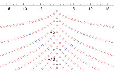
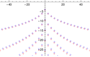
Figure 2. Left: resonances for the ball of radius one in ${\mathbb{R}}^{3}$. For each spherical momentum $\ell$ they are given by solutions of $H^{(2)}_{\ell+1/2}(\lambda)=0$ where $H^{(2)}_{\nu}$ is the Hankel function of the second kind and order $\nu$. Each zero appears as a resonance of multiplicity $2\ell+1$; highlighted are resonances corresponding to $\ell=12$. Right: resonances of the ball with radius $R=0.25$ in ${\mathbb{H}}^{3}$ (red) and in ${\mathbb{R}}^{3}$ (blue); this illustrates Theorem 3.

We expect that $\mu=1$ in (1.6). (An adaptation of Ralston’s argument [Ra78] should work but would require some buildup of scattering theory; for a proof of his crucial estimate without using Lax–Phillips theory, see [DyZw, Exercise 3.5].) That the estimate (1.6) is independent of $\kappa$ is related to rescaling: identifying an obstacle with a subset of ${\mathbb{R}}^{n}$ and denoting by $x\mapsto\varepsilon x$ the Euclidean dilation, we see that if $\sigma\in\operatorname{Res}(\varepsilon\mathcal{O},1)$ then $\varepsilon\sigma\in\operatorname{Res}(\mathcal{O},\varepsilon)$, and $\varepsilon\sigma$ should be close to a resonance in $\operatorname{Res}(\mathcal{O},0)$. So even though the bound (1.5) gets worse for small $\kappa$, the bound in odd dimensions is close to (1.4) and improves for small diameters. This is illustrated by Fig. 2 and confirmed by the following theorem:

Theorem 3.

Suppose that $\mathcal{O}\subset{\mathbb{H}}_{\kappa}^{n}\simeq{\mathbb{R}}^{n}$ is an arbitrary bounded obstacle with smooth boundary and that $n\geq 3$ is odd. Then

$$\operatorname{Res}({\mathcal{O}},\kappa)\to\operatorname{Res}({\mathcal{O}},0),\ \ \ \kappa\to 0,$$

locally uniformly and with multiplicities.

A more precise version is given in Theorem 7 in §7.

Acknowledgments. We would like to thank Steve Zelditch whose comments on [Zw17] provided motivation for this project, and Volker Schlue for useful discussions. We would also like to thank an anonymous referee for a careful reading of the manuscript and a number of valuable suggestions which in particular led to the addition of §6.3. PH is grateful to the Miller Institute at the University of California, Berkeley for support, and MZ acknowledges partial support under the National Science Foundation grant DMS-1500852. This research was partially conducted during the period PH served as a Clay Research Fellow.

2. Resonances for balls in ${\mathbb{H}}_{\kappa}^{n}$

As motivation for the proofs of the main results we present computations of resonances of the geodesic ball of radius $R$ in ${\mathbb{H}}^{n}_{\kappa}$, with Dirichlet boundary conditions. (See also Borthwick [Bo10].)

The starting point is the calculation

$$s_{\kappa}^{\frac{n-1}{2}}\Bigl{(}-\Delta_{{\mathbb{H}}^{n}_{\kappa}}-\Bigl{(}\frac{n-1}{2}\Bigr{)}^{2}\kappa^{2}-\sigma^{2}\Bigr{)}s_{\kappa}^{-\frac{n-1}{2}}=D_{r}^{2}+s_{\kappa}^{-2}\Bigl{(}-\Delta_{{\mathbb{S}}^{n-1}}+\frac{(n-1)(n-3)}{4}\Bigr{)}-\sigma^{2}$$

for $s_{\kappa}(r)=\kappa^{-1}\sinh(\kappa r)$, see Lemma 4.1 below. Decomposing into spherical harmonics and using that the eigenvalues of ${\mathbb{S}}^{n-1}$ are given by $\ell(\ell+n-2)$, $\ell\in{\mathbb{Z}}_{\geq 0}$, it suffices to study the radial operator

$$P_{n,\ell}(\sigma):=D_{r}^{2}+s_{\kappa}^{-2}\Bigl{(}\frac{(n-1)(n-3)}{4}+\ell(\ell+n-2)\Bigr{)}-\sigma^{2}.$$

Our objective is to calculate non-trivial solutions of $P_{n,\ell}(\sigma)u=0$ which are outgoing, which means that $u=e^{ir\sigma}v(\coth\kappa r)$, where $v=v(x)$, $x=\coth\kappa r$, is smooth in $[1,\infty)_{x}$ down to $x=1$. (This is precisely the condition (3.1) in Theorem 4 below, after rescaling to the case $\kappa=1$.) The space of such $u$ is a 1-dimensional space, and if, for fixed $\sigma$, such a $u$ vanishes at $r=R$, then $\sigma$ is a resonance for the $R$-ball in ${\mathbb{H}}^{n}_{\kappa}$. By direct computation, we have

$$P_{n+2,\ell-1}(\sigma)=P_{n,\ell}(\sigma),$$

hence $P_{n,\ell}=P_{n+2\ell,0}$, and it suffices to calculate outgoing solutions $u$ of $P_{n,0}(\sigma)u=0$ for all $n\geq 2$. Using $(\sinh\kappa r)^{-2}=x^{2}-1$, one finds that $e^{-ir\sigma}P_{n,0}(\sigma)e^{ir\sigma}v(\coth\kappa r)=0$ is equivalent to

$$\tilde{P}_{n}(\sigma)v:=\Bigl{(}\partial_{x}(1-x^{2})\partial_{x}+2i\kappa^{-1}\sigma\partial_{x}+\frac{(n-1)(n-3)}{4}\Bigr{)}v=0$$

Changing variables $y=(1-x)/2$, this is a hypergeometric equation. For odd $n=2k+1$, smooth solutions of this equation are polynomials of $x$. To see this directly, we make the ansatz

$$v(x)=\sum_{j=0}^{\infty}\frac{(x-1)^{j}}{\Gamma(j+1-i\kappa^{-1}\sigma)}c_{k,j},\quad c_{k,0}=1;$$

plugged into the ODE, this yields the recursion relation

$$c_{k,j}=\frac{k(k-1)-j(j-1)}{2j}c_{k,j-1},\ \ j\geq 1,$$

in particular $c_{k,j}=0$ for all $k\geq j$. Therefore, multiplying through by $\Gamma(k-i\kappa^{-1}\sigma)$ in order to deal with integer coincidences $k-i\kappa^{-1}\sigma\in{\mathbb{Z}}_{<0}$, the non-trivial outgoing solution $u_{n}(r;\sigma)$ of $P_{n}(\sigma)u_{n}(r;\sigma)=0$, $n=2k+1$, is given by

$$u_{2k+1}(r;\sigma)=e^{ir\sigma}\sum_{j=0}^{k-1}\frac{(\coth(\kappa r)-1)^{j}}{2^{j}j!}\prod_{l=1}^{j}\bigl{(}k(k-1)-l(l-1)\bigr{)}\prod_{m=j+1}^{k-1}(m-i\kappa^{-1}\sigma),$$

where the product $\prod_{l=1}^{0}$ is defined to be $1$.

Note that $e^{-ir\sigma}u_{2k+1}(r;\sigma)$ is a polynomial in $\sigma$ of degree $k-1$. If the size $R$ of the obstacle is fixed, the zeros of $u_{2k+1}(R;\sigma)=0$ are the resonances. See Fig. 2.

Suppose now the obstacle is large, so $\coth\kappa R$ is close to $1$, and fix $k$. Then $u_{2k+1}(R;\sigma)$, as a function of $\sigma$, is well-approximated by a constant multiple of

$$e^{iR\sigma}\prod_{m=1}^{k-1}(m-i\kappa^{-1}\sigma),$$

whose zeros are located at $-i\kappa m$, $m=1,\ldots,k-1$. By Rouché’s theorem, this implies that for $n$ odd, $\kappa>0$, and $\varepsilon>0$ fixed, there exists $R_{0}>0$ such that for spherical obstacles in ${\mathbb{H}}^{n}_{\kappa}$ with radius $R>R_{0}$, there exists a resonance $\sigma$ with $|\sigma+i\kappa|<\varepsilon$. (For comparison, Theorem 1 only gives $\operatorname{Im}\sigma\leq-\kappa/2$.)

One can also numerically compute resonances on even-dimensional hyperbolic spaces – see Fig. 1. When the diameter of a spherical obstacle in ${\mathbb{H}}^{2}$ tends to zero, numerical experiments suggest that the topmost resonance converges to $-i/2$, the topmost resonance for the free resolvent on ${\mathbb{H}}^{2}$.

3. Preliminaries

In this section we review the meromorphic continuation of the resolvent on asymptotically hyperbolic manifolds with obstacles, resonance free strips and resonance expansions in the non-trapping case, and the vector field approach via the stress–energy tensor.

3.1. Meromorphic continuation of the resolvent

Let $(M,g)$ be an (even) asymptotically hyperbolic manifold with boundary. This means that $M$ admits a compactification to a manifold $\bar{M}$ with boundary $\partial\bar{M}=\partial M\cup\partial_{1}\bar{M}$, where $\partial_{1}\bar{M}$ is the conformal boundary of $M$; moreover, the Riemannian metric $g$ is smooth on $M$, while in a collar neighborhood $[0,\varepsilon)_{x}\times(\partial_{1}\bar{M})_{y}$ of the conformal boundary, the rescaled metric $\bar{g}(x,y,dx,dy):=x^{2}g(x,y,dx,dy)$ is a smooth Riemannian metric on $\bar{M}$ whose Taylor expansion $x=0$ contains only even powers of $x$ (see also [Gui05]), and $|dx|_{\bar{g}}^{2}=1$ at $\partial_{1}\bar{M}$. See [DyZw, §5.1] for further discussion.

An example considered in this paper is $(M,g)=(\mathbb{H}_{1}^{n}\setminus\mathcal{O},g_{1})$. We discuss the conformal compactification and its smooth structure explicitly in §6.2.

The following theorem is essentially due to Vasy [Va12, Va13] – see also [Zw16] for a shorter self-contained presentation:

Theorem 4.

Suppose that $P:=-\Delta_{g}-(\frac{n-1}{2})^{2}$ and that $R(\lambda):=(P-\lambda^{2})^{-1}\colon L^{2}(M)\to L^{2}(M)$, $\operatorname{Im}\lambda>0$ is the resolvent. Then $R(\lambda)$ continues meromorphically as an operator

$$R(\lambda):{C^{\infty}_{\rm{c}}}(M)\to{C^{\infty}}(M).$$

Moreover, if $\lambda$ is a resonance of $P$, then there exists a non-trivial solution (resonant state) $v$ of $(P-\lambda^{2})v=0$ which satisfies

$$\tilde{v}=x^{\frac{n-1}{2}-i\lambda}v,\ \ v\in{C^{\infty}}(\bar{M}_{\mathrm{even}}),$$ (3.1)

where $\bar{M}_{\mathrm{even}}=\bar{M}$ as topological spaces, but where smooth functions on $\bar{M}_{\mathrm{even}}$ (the ‘even compactification’) are precisely those smooth functions on $\bar{M}$ which are smooth in $x^{2}$ near $\partial_{1}\bar{M}$.

For $(M,g)=({\mathbb{H}}_{1}^{n}\setminus{\mathcal{O}},g_{1})$, this is also discussed in [Bo10]. By rescaling, Theorem 4 applies to $({\mathbb{H}}_{\kappa}^{n}\setminus\mathcal{O},g_{\kappa})$ as well, with $P=P_{\kappa}$ given by (1.2) and the resolvent denoted by $R_{\kappa}(\lambda)$. The multiplicity of a non-zero resonance $\lambda$ of $P_{\kappa}$ is then defined as

$$m_{\kappa}(\lambda)=\dim\Bigl{[}\Bigl{(}\oint_{\lambda}R_{\kappa}(\zeta)\,d\zeta\Bigr{)}(L^{2}_{\mathrm{comp}}({\mathbb{H}}^{n}_{\kappa}\setminus{\mathcal{O}}))\Bigr{]},$$ (3.2)

where the contour is a small circle around $\lambda$, traversed counter-clockwise, which does not contain any other resonances.

3.2. Resonance free strips for non-trapping obstacles for general hyperbolic ends

The estimates on resonance width, $|\operatorname{Im}\lambda|$, will be obtained by studying local energy decay (see [Mo72, FeLa90, HiZw17] for arguments which use the resonant states directly). The most conceptual way of relating energy decay to resonances is via resonance expansions of waves; we will discuss this for general non-trapping obstacles on manifolds with asymptotically hyperbolic ends. In §6.3, we shall prove that star-shaped obstacles in hyperbolic space are non-trapping.

For $M$ given in §3.1, Melrose–Sjöstrand [MeSj78, MeSj82] (see also [Hö85, Definition 24.3.7]) defined the broken geodesic flow. We make a general assumption here that the geodesics do not have points of infinite tangency to $\partial M$.

A combination of [Bu02, Propositions 4.4, 4.6, Proof of Theorem 1.3] (see also [BuLe01, §3.3]) and [DyZw, Theorems 6.14, 6.15] immediately gives

Theorem 5.

Suppose that $(M,g)$ is an asymptotically hyperbolic manifold with boundary. We assume that the geodesics do not have points of infinite tangency to $\partial M$, and that the broken geodesic flow is non-trapping, that is, each geodesic leaves any compact set. Then for any $\alpha>0$ and $\chi\in{C^{\infty}_{\rm{c}}}(M)$ there exists $C>0$ such that

$${\operatorname{Im}\lambda>-\alpha},\ \ {\operatorname{Re}\lambda\geq C}\ \Longrightarrow\ \|\chi R(\lambda)\chi\|\leq C|\lambda|^{-1}.$$ (3.3)

In particular, there are only finitely many poles of $R(\lambda)$ in any strip $\operatorname{Im}\lambda>-\alpha$.

Remark 3.1.

In the case of $\mathbb{H}_{\kappa}^{n}\setminus\mathcal{O}$ we could get a stronger result using Vainberg’s method [Va73] (see also [DyZw, §4.6]): namely a logarithmically large resonance free region. Since that improvement is not necessary for our arguments we opted for a more general version.

This immediately implies resonance expansions, see for example [Zw12, Proof of Theorem 5.10]:

Theorem 6.

Let $(M,g)$ be an asymptotically hyperbolic manifold satisfying the assumptions of Theorem 5. Suppose that $u(t,x)$ is the solution of

$$(D_{t}^{2}-P_{k})u(t,x)=0\ \text{in}\ {\mathbb{R}}\times({\mathbb{H}}^{n}_{\kappa}\setminus\mathcal{O}),\ \ u(t,x)=0\ \text{on}\ {\mathbb{R}}\times\partial\mathcal{O},$$

$$u(0,x)=u_{0}(x)\in H^{1}_{\mathrm{comp}}({\mathbb{H}}^{n}_{\kappa}\setminus\mathcal{O}),\ \ \partial_{t}u(0,x)=u_{1}(x)\in L^{2}_{\mathrm{comp}}({\mathbb{H}}^{n}_{\kappa}\setminus\mathcal{O}).$$

Denote by $\{\lambda_{j}\}\subset{\mathbb{C}}$ the set of resonances of $P_{\kappa}$. Then, for any $A>0$,

$$u(t,x)=\sum_{\operatorname{Im}\lambda_{j}>-A}\sum_{\ell=0}^{m_{\kappa}(\lambda_{j})-1}t^{\ell}e^{-i\lambda_{j}t}u_{j,\ell}(x)+E_{A}(t),$$

where the sum is finite,

$$\sum_{\ell=0}^{m_{\kappa}(\lambda_{j})-1}t^{\ell}e^{-i\lambda_{j}t}u_{j,\ell}(x)=\operatorname{Res}_{\lambda=\lambda_{j}}\bigl{(}e^{-i\lambda t}(iR_{\kappa}(\lambda)u_{1}+\lambda R_{\kappa}(\lambda)u_{0})\bigr{)},$$

$(P_{\kappa}-\lambda_{j}^{2})^{k+1}u_{j,k}=0$, and for any $K>0$ such that $\operatorname{supp}u_{j}\subset B(0,K)$, there exist constants $C_{K,A}$ and $T_{K,A}$ such that

$$\|E_{A}(t)\|_{H^{1}(B(0,K))}\leq C_{K,A}e^{-At}(\|u_{0}\|_{H^{1}}+\|u_{1}\|_{L^{2}}),\ \ t\geq T_{K,A}.$$

The remainder $E_{A}$ is only estimated in $H^{1}$ because (3.3) only gives a strip free of resonances, rather than a logarithmic region.

3.3. Energy-stress tensor and the vector field method

We briefly recall the general formalism for obtaining energy estimates, referring to [Ta11a, §2.6] and [DaRo08, §4.1.1] for detailed presentations (see also [Dy11, §1.1] for a concise discussion relevant here). The general setting we use here makes the formulas more accessible and will be particularly useful in §4.

Let $M$ be an $(n+1)$-dimensional smooth manifold and $G$ a Lorentzian metric on $M$, that is, a symmetric $(0,2)$-tensor of signature $(n,1)$. The volume form, gradient, and divergence are defined as in Riemannian geometry, and they give the d’Alembertian, $\Box_{G}u={\rm{div}}_{G}(\nabla_{G}u)$. The stress–energy tensor for a Klein–Gordon operator $\Box_{G}-m^{2}$ is a symmetric $(0,2)$-tensor associated to $u\in{C^{\infty}}(M)$:

$$T_{u}(X,Y):=G(X,\nabla_{G}u)G(Y,\nabla_{G}u)-{\textstyle\frac{1}{2}}(G(\nabla_{G}u,\nabla_{G}u)+m^{2}u^{2})G(X,Y),$$

$X,Y\in{C^{\infty}}(M;TM)$. To $T_{u}$ and a vector field $V$ we associate the current $J^{V}(u)\in{C^{\infty}}(M;TM)$ by demanding that for all vector fields $X$,

$$G(J^{V}(u),X)=T_{u}(V,X).$$

The key identity is

$$(\Box_{G}-m^{2})u\,Vu+K^{V}(\nabla_{G}u,\nabla_{G}u)-{\textstyle\frac{1}{4}}m^{2}u^{2}\operatorname{tr}_{G}(\mathcal{L}_{V}G)={\rm{div}}_{G}\,J^{V}(u),$$

where

$$K^{V}:={\textstyle\frac{1}{2}}\mathcal{L}_{V}G-{\textstyle\frac{1}{4}}G\operatorname{tr}_{G}(\mathcal{L}_{V}G).$$

The simplest version of this identity arises in the case that $V$ is a Killing vector field, i.e. satisfies $\mathcal{L}_{V}G=0$. In this case the divergence theorem gives

$$(\Box_{G}-m^{2})u=0,\ \ \mathcal{L}_{V}G=0\ \Longrightarrow\ \int_{\partial\Omega}G(J^{V}(u),\mathbf{n})\,dS=0,$$ (3.4)

where $\Omega\subset M$ is an open subset with smooth boundary, $\mathbf{n}$ is the unit outward normal vector and $dS$ is the measure induced on $\partial\Omega$ by $d\!\operatorname{vol}_{G}$. The outward unit normal vector is defined by the conditions

$$G(\mathbf{n},\mathbf{n})=1,\ \ G(\mathbf{n},X)>0,$$

for any vector field $X$ pointing out of $\Omega$. It may blow up for null hypersurfaces, but this is then compensated by the vanishing of $dS$ – see [DaRo08, Appendix C].

4. Morawetz estimates in hyperbolic space

We will now apply the general formalism recalled in §3.3 to scattering by obstacles. It follows the approach of Morawetz [Mo66a, Mo66b], see also [LaPh68, Appendix 3], to Euclidean scattering. However, our derivation of the generalization of her fundamental identity [Mo66b, Lemma 3] seems slightly different.

4.1. Conjugated equation and a weighted energy inequality

The Lorentzian metric corresponding to the metric (1.1) is given by

$$\tilde{g}_{\kappa}=-dt^{2}+g_{\kappa},$$ (4.1)

and we define

$$\Box_{\kappa}:=\Box_{\tilde{g}_{\kappa}}+\kappa^{2}\left(\frac{n-1}{2}\right)^{2}.$$ (4.2)

We then consider a conjugated operator, described in the following lemma; it was already used implicitly in §2. When no confusion is likely we write

$$s=s_{\kappa},\ \ g=g_{\kappa},\ \ \tilde{g}=\tilde{g}_{\kappa}.$$

Lemma 4.1.

With the notation of (1.1) and (4.2), we have

$$s^{2}s^{\frac{n-1}{2}}\Box_{\kappa}s^{-\frac{n-1}{2}}=\Box_{G}-\frac{(n-1)(n-3)}{4},$$ (4.3)

where

$$G=G_{\kappa}:=s(r)^{-2}(-dt^{2}+dr^{2})+h.$$ (4.4)

In addition, if $w:=s^{\frac{n-1}{2}}u$, then

$$\begin{split}&\left(u_{t}^{2}+|\nabla_{g}u|^{2}-\kappa^{2}\left(\tfrac{n-1}{2}\right)^{2}u^{2}\right)d\!\operatorname{vol}_{g}\\ &\ \ \ \ =\left(w_{t}^{2}+w_{r}^{2}+s^{-2}|\nabla_{h}w|^{2}_{h}+s^{-2}\tfrac{(n-1)(n-3)}{4}w^{2}\right)dr\,d\!\operatorname{vol}_{h}-\left(\tfrac{n-1}{2}\tfrac{s^{\prime}}{s}w^{2}\right)_{r}dr\,d\!\operatorname{vol}_{h}.\end{split}$$ (4.5)

Proof.

Since $|\det\tilde{g}|=s^{2(n-1)}$, we have $\Box_{\tilde{g}}=-\partial_{t}^{2}+s^{-{n-1}}\partial_{r}s^{{n-1}}\partial_{r}+s^{-2}\Delta_{h}$. Hence we only need to compute

$$\begin{split}s^{\frac{n-1}{2}}(s^{-{n-1}}\partial_{r}s^{{n-1}}\partial_{r})s^{-\frac{n-1}{2}}&=(s^{-\frac{n-1}{2}}\partial_{r}s^{\frac{n-1}{2}})(s^{\frac{n-1}{2}}\partial_{r}s^{-\frac{n-1}{2}})\\ &=\textstyle\left(\partial_{r}+{{\frac{n-1}{2}}\frac{s^{\prime}}{s}}\right)\left(\partial_{r}-{{\frac{n-1}{2}}\frac{s^{\prime}}{s}}\right)\\ &=\textstyle\partial_{r}^{2}-\frac{(n-1)^{2}}{4}\frac{s^{\prime 2}}{s^{2}}-\frac{n-1}{2}\frac{s^{\prime\prime}s-s^{\prime 2}}{s^{2}}\\ &=\textstyle\partial_{r}^{2}-\frac{(n-1)(n-3)}{4s^{2}}-\kappa^{2}\left(\frac{n-1}{2}\right)^{2}.\end{split}$$ (4.6)

Multiplying by $s^{2}$ gives (4.3). (We direct the reader to (6.12) for a more conceptual point of view.) To establish (4.5), it again suffices to consider radial derivatives:

$$\begin{split}(u_{r}^{2}-\kappa^{2}(\tfrac{n-1}{2})^{2}u^{2})s^{n-1}&=s^{n-1}(s^{-\frac{n-1}{2}}w)_{r}^{2}-\kappa^{2}(\tfrac{n-1}{2})^{2}w^{2}\\ &=(w_{r}-\tfrac{n-1}{2}\tfrac{s^{\prime}}{s}w)^{2}-\kappa^{2}(\tfrac{n-1}{2})^{2}w^{2}\\ &=w_{r}^{2}-(\tfrac{n-1}{2}\tfrac{s^{\prime}}{s}w^{2})_{r}+\left(\tfrac{n-1}{2}\left(\tfrac{s^{\prime}}{s}\right)_{r}+\left(\tfrac{n-1}{2}\right)^{2}\left(\tfrac{s^{\prime}}{s}\right)^{2}-\kappa^{2}\left(\tfrac{n-1}{2}\right)^{2}\right)w^{2}\\ &=w_{r}^{2}+\tfrac{(n-1)(n-3)}{4s^{2}}w^{2}-(\tfrac{n-1}{2}\tfrac{s^{\prime}}{s}w^{2})_{r},\end{split}$$

where we used the same computation as in (4.6). Since $d\!\operatorname{vol}_{g_{\kappa}}=s^{n-1}drd\!\operatorname{vol}_{h}$, (4.5) follows. ∎

4.2. An energy identity

We now calculate the stress–energy tensor given by (4.4) for the metric $G$ and for $m^{2}=\frac{(n-1)(n-3)}{4}$ in terms of the decomposition of vectors into components of $\partial_{t}$, $\partial_{r}$, and vectors tangent to the sphere:

$$T_{u} =\begin{bmatrix}u_{t}^{2}&u_{r}u_{t}&u_{t}\nabla_{h}u^{T}\\ u_{r}u_{t}&u_{r}^{2}&u_{r}\nabla_{h}u^{T}\\ \nabla_{h}uu_{t}&\nabla_{h}uu_{r}&\nabla_{h}u\nabla_{h}u^{T}\end{bmatrix}$$

$$\qquad\qquad-\frac{s^{2}(-u_{t}^{2}+u_{r}^{2})+|\nabla_{h}u|_{h}^{2}+m^{2}|u|^{2}}{2}\begin{bmatrix}-s^{-2}&0&0\\ 0&s^{-2}&0\\ 0&0&1\end{bmatrix}.$$

Let $V:=a(t,r)\partial_{t}+b(t,r)\partial_{r}$. Then the orthogonal decomposition of $J^{V}(u)$ with respect to $dt^{2}+dr^{2}+h$ is given by

$$\begin{split}J^{V}(u)&=\begin{bmatrix}-s^{2}&0&0\\ 0&s^{2}&0\\ 0&0&1\end{bmatrix}T_{u}\begin{bmatrix}a\\ b\\ 0\end{bmatrix}\\ &=\textstyle{\frac{1}{2}}\begin{bmatrix}-s^{2}(au_{t}^{2}+2bu_{r}u_{t}+au_{r}^{2})-a|\nabla_{h}u|_{h}^{2}-am^{2}|u|^{2}\\ s^{2}(bu_{r}^{2}+2au_{r}u_{t}+bu_{t}^{2})-b|\nabla_{h}u|_{h}^{2}-bm^{2}|u|^{2}\\ {2}au_{t}\nabla_{h}u+{2}bu_{r}\nabla_{h}u\end{bmatrix}.\end{split}$$ (4.7)

We now calculate

$$\mathcal{L}_{V}G=2s^{-2}\left((-a_{t}+bs^{\prime}/s)dt^{2}+(b_{t}-a_{r})dtdr+(b_{r}-bs^{\prime}/s)dr^{2}\right),$$

and hence for $V$ to be a Killing vector field, we need to find $a=a(t,r)$ and $b=b(t,r)$ such that

$$a_{t}=b_{r},\ \ a_{r}=b_{t},\ \ b_{r}=bs^{\prime}/s.$$ (4.8)

An obvious choice is $a=1$, $b=0$, which in the context of the identity (3.4) gives energy conservation. As will be clear later, a convenient choice for the purpose of proving generalized Morawetz (local energy decay) estimates is given by

$$a:=2\kappa^{-2}(\cosh\kappa r\cosh\kappa t-1),\ \ b:=2\kappa^{-2}\sinh\kappa r\sinh\kappa t.$$ (4.9)

Suppose that $w\in C({\mathbb{R}};H^{1}_{{{\mathrm{comp}}}}({\mathbb{H}}_{k}^{n}\setminus\mathcal{O}))$. We will use the following notation:

$$\begin{split}&F_{a,b}(w,T,R):=\\ &\ \ \ \int_{B(0,R)\setminus\mathcal{O}}\left(aw_{t}^{2}+2bw_{t}w_{r}+aw_{r}^{2}+as^{-2}|\nabla_{h}u|^{2}_{h}+as^{-2}m^{2}w^{2}\right)dr\,d\!\operatorname{vol}_{h}|_{t=T},\end{split}$$ (4.10)

$$F_{a,b}(w,t):=F_{a,b}(w,t,\infty),\ \ B(0,\infty):=\mathbb{H}^{n}_{\kappa}.$$

An application of (3.4) then gives

Lemma 4.2.

Suppose that $a=a(r,t)$ and $b=b(r,t)$ satisfy (4.8) and that $F_{a,b}$ is defined by (4.10). Suppose that $w\in C({\mathbb{R}};H_{{\mathrm{comp}}}^{1}({\mathbb{H}}^{n}_{\kappa}\setminus\mathcal{O}))$ satisfies

$$(\Box_{G}-m^{2})w(t,x)=0,\ \ x\in\mathbb{H}_{\kappa}^{n}\setminus\mathcal{O},\ \ w(t,x)=0,\ \ x\in\partial\mathcal{O}.$$

Then

$$F_{a,b}(w,T)=F_{a,b}(w,0)-\int_{0}^{T}\int_{\partial\mathcal{O}}b(t,r)g(\nu,\nabla_{g}r)g(\nu,\nabla_{g}w)^{2}s(r)^{-n+1}d\sigma_{g}\,dt,$$ (4.11)

where $g=g_{\kappa}$ is given by (1.1), $\nu$ is the outward unit (with respect to $g$) normal vector and $d\sigma_{g}$ is the measure induced by $g$ on $\partial\mathcal{O}$.

Proof.

Since $\mathcal{O}$ is star-shaped (with respect to the origin, as can be assumed without loss of generality) we can write

$$\partial\mathcal{O}=\{x=r\omega:r=f(\omega),\ \omega\in{\mathbb{S}}^{n-1}\}$$

for some $f:{\mathbb{S}}^{n-1}\to(0,\infty)$. To obtain (4.11), we apply (3.4) to $\Omega=[0,T]\times({\mathbb{H}}^{n}_{\kappa}\setminus\mathcal{O})$,

$$\partial\Omega=\Gamma_{1}\cup\Gamma_{2},\ \ \ \Gamma_{1}:=[0,T]\times\partial\mathcal{O},\ \ \Gamma_{2}:=\{0,T\}\times({\mathbb{H}}^{n}_{\kappa}\setminus\mathcal{O}).$$

On $\Gamma_{1}$ (in the notation of (4.7)),

$$\mathbf{n}=-\nabla_{G}(r-f)/|\nabla_{G}(r-f)|_{G}=[0,-s^{2},\nabla_{h}f](s^{2}+|\nabla_{h}f|^{2}_{h})^{-\frac{1}{2}},\ \ s=s(f(\omega)),$$

$$dS=s^{-2}(s^{2}+|\nabla_{h}f|^{2}_{h})^{\frac{1}{2}}d\operatorname{vol}_{h}dt,$$

$$\begin{split}g(J^{V}(w),\mathbf{n})&=-{\textstyle\frac{1}{2}}b(s^{2}w_{r}^{2}-|\nabla_{h}w|_{h}^{2}-{2}w_{r}\langle\nabla_{h}w,\nabla_{h}f\rangle_{h})(s^{2}+|\nabla_{h}f|^{2}_{h})^{-\frac{1}{2}}\\ &=-{\textstyle\frac{1}{2}}{{bw_{r}^{2}}}(s^{2}+|\nabla_{h}f|^{2}_{h})^{{\frac{1}{2}}},\end{split}$$

where we used the boundary condition $w(t,f(\omega),\omega)\equiv 0$ (thus $w_{t}(t,f(\omega),\omega)=0$ and $(\nabla_{h}w)(t,f(\omega),\omega)=-w_{r}\nabla_{h}f(\omega)$.) On $\Gamma_{2}$,

$$\mathbf{n}=\pm[s,0,0],\ \ dS=s^{-1}drd\!\operatorname{vol}_{h},$$

$$g(J^{V}(w),\mathbf{w})=\mp{\textstyle{\frac{1}{2}}}s\left(aw_{t}^{2}+bw_{r}w_{t}+aw_{r}^{2}+as^{-2}|\nabla_{h}w|^{2}_{h}+am^{2}|w|^{2}\right).$$

Hence, (3.4) gives

$$F_{a,b}(w,T)=F_{a,b}(w,0)-\int_{0}^{T}\int_{{\mathbb{S}}^{n-1}}b(t,f(\omega))(1+s^{-2}|\nabla_{h}f|^{2}_{h})w_{r}(f(\omega),\omega)^{2}\,d\!\operatorname{vol}_{h}dt.$$

The more invariant form given in (4.11) follows from explicit expressions:

$$\nu=(1+s^{-2}|\nabla_{h}f|^{2}_{h})^{-\frac{1}{2}}(1,-s^{-2}\nabla_{h}f),\ \ d\sigma_{g}=s^{n-1}(1+s^{-2}|\nabla_{h}f|^{2}_{h})^{\frac{1}{2}}d\operatorname{vol}_{h},$$

and $g(\nu,\nabla_{g}w)=w_{r}(1+s^{-2}|\nabla_{h}f|^{2})^{\frac{1}{2}}$. ∎

We remark that (4.11) is valid for any obstacle $\mathcal{O}$; the assumption that $\partial\mathcal{O}$ be star-shaped implies however that the second term on the right hand side is negative.

4.3. Proof of Theorem 1 for $n\geq 3$

Let $a,b$ be given by (4.9). Lemmas 4.1 and 4.2 give the following energy inequality: Suppose that, in the notation (4.2),

$$\Box_{\kappa}u=0\ \text{ in }\ [0,T]\times\mathbb{H}_{\kappa}^{n}\setminus\mathcal{O},\ \ u=0\ \text{ on }\ [0,T]\times\partial\mathcal{O},$$

$$(u(0,x),u_{t}(0,x))\in(H^{1}\times L^{2})(\mathbb{H}_{\kappa}^{n}\setminus\mathcal{O}),$$

and define

$$E_{a,b}(u,t,r):=F_{a,b}(s^{\frac{n-1}{2}}u,t,r),\ \ E_{a,b}(u,t):=E_{a,b}(u,t,\infty),$$ (4.12)

then we have

$$E_{a,b}(u,t)\leq E_{a,b}(u,0),\ \ t\geq 0.$$

We now assume that

$$\operatorname{supp}\partial_{t}^{k}u(0,\bullet)\subset B(0,R),\ \ k=0,1.$$

Since for any $a,b\geq 0$,

$$(a-b)(x^{2}+y^{2})\leq ax^{2}+2bxy+ay^{2}\leq(a+b)(x^{2}+y^{2})$$

and since for $n\geq 3$, $m^{2}=(n-1)(n-3)/4\geq 0$, we then have

$$E_{c,0}(u,t,R)\leq E_{a,b}(u,t,R),\ \ t\geq 0,$$

$$c(t,r):=a(t,r)-b(t,r)=2\kappa^{-2}(\cosh\kappa(t-r)-1)$$

Hence for $t\geq R$, and using that $a=c$ and $b=0$ at $t=0$,

$$\begin{split}c(t,R)E_{1,0}(u,t,R)&\leq E_{c,0}(u,t,R)\leq E_{a,b}(u,t,R)\\ &\leq E_{a,b}(u,0)=E_{c,0}(u,0)\leq c(0,R)E_{1,0}(u,0).\end{split}$$

We obtain for $t>2R$:

$$E_{1,0}(u,t,R)\leq\frac{\cosh\kappa R-1}{\cosh\kappa(t-R)-1}E_{1,0}(u,0)\leq Ce^{-\kappa t}E_{1,0}(u,0).$$ (4.13)

The results of §3.2 then give Theorem 1. This crucially uses that $E_{1,0}(u,t,R)$ is coercive (unlike the integral of the natural energy density for $u$, given by the left hand side of the identity (4.5), over $B(0,R)\setminus\mathcal{O}$).

We note that the second part of Lemma 4.1 shows that for the quantity

$$\mathcal{E}(u,t,R):=\int_{B(0,R)\setminus\mathcal{O}}\left(u_{t}^{2}+|\nabla_{g}u|^{2}-\kappa^{2}\left(\tfrac{n-1}{2}\right)^{2}u^{2}\right)\,d\mathrm{vol}_{g}\,|_{t=T},$$

$\mathcal{E}(u,T):=\mathcal{E}(u,T,\infty)$, we have

$$\mathcal{E}(u,t)=E_{1,0}(u,t),\ \ \mathcal{E}(u,t,R)\leq E_{1,0}(u,t,R).$$

However, $\mathcal{E}(u,t,R)$ is only coercive when $\kappa=0$, and in this case, the argument leading to (4.13) gives the estimate of Morawetz:

$$\mathcal{E}(u,t,R)\leq\frac{R^{2}}{(t-R)^{2}}\mathcal{E}(u,0),$$ (4.14)

when the initial data have support in $B(0,R)\setminus\mathcal{O}$.

5. Improved estimates in odd dimensions

We now revisit the argument of Morawetz for obtaining exponential decay in odd dimensions. We use the notation of (1.1) and (4.2) and we denote by $\nabla_{\kappa}$, $|\bullet|_{\kappa}$ the gradient and norm with respect to the Riemannian metric on ${\mathbb{H}}^{n}_{\kappa}$. We recall that the obstacle $\mathcal{O}$ is star-shaped with respect to the origin $0\in{\mathbb{H}}^{n}_{\kappa}$, and we assume that $\mathcal{O}$ is contained in the ball $B(0,\rho)$.

The key fact is the strong Huyghens principle illustrated in Fig. 3: suppose that

$$\Box_{\kappa}u=F,\ F\in\mathcal{D}^{\prime}({\mathbb{R}}\times{\mathbb{H}}^{n}_{\kappa}),\ \ u(t,x)|_{t<0}=0;$$

if

$$\Gamma_{(t,x)}^{-}:=\{(t^{\prime},x^{\prime})\colon t^{\prime}\leq t,\ d_{\kappa}(x,x^{\prime})=t-t^{\prime}\}$$

then

$$\Gamma_{(t,x)}^{-}\cap\operatorname{supp}F=\emptyset,\ \ \Longrightarrow\ u(t,x)=0.$$ (5.1)

Figure 3. If $\Box_{\kappa}u=F$ in ${\mathbb{R}}_{+}\times{\mathbb{H}}_{\kappa}^{n}$, $n\geq 3$, odd, and $F$ is supported in $B_{T,\rho}:=[0,T]\times B(0,\rho)$ (shaded region), and $u|_{t=0}$ and $\partial_{t}u|_{t=0}$ are supported in $B(0,T+\rho)$, then $u(t,x)\equiv 0$ for $|x|\leq t-(T+\rho)$.

We will make use of the (local) energy

$$E(u,t,r):=E_{1,0}(u,t,r),\ \ E(u,t):=E(u,t,\infty),$$

defined using (4.12). For $u(t,\bullet)$ defined on $\mathbb{H}^{n}_{\kappa}$, we can also integrate over $B(0,r)$ and we denote the corresponding energies by $E_{0}(u,t,r)$, $E_{0}(u,t)$.

We will now consider

$$\begin{gathered}\Box_{\kappa}u=0\ \text{on}\ [0,\infty)\times{\mathbb{H}}^{n}_{\kappa}\setminus\mathcal{O},\ \ u|_{(0,\infty)\times\partial\mathcal{O}}=0\\ \operatorname{supp}\partial_{t}^{k}u|_{t=0}\subset B(0,R),\ \ \partial_{t}^{k}u|_{t=0}\in H^{1-k}({\mathbb{H}}^{n}_{\kappa}\setminus\mathcal{O}),\ \ k=0,1.\end{gathered}$$ (5.2)

For solutions $u$, the energy $E(u,t)$ does not depend on time.

Lemma 5.1.

Let $u$ be the solution to the initial value problem (5.2) with $R=3\rho$. Then for any $T\geq 2\rho$, we have a decomposition

$$\begin{gathered}u(t,x)=u_{T}(t,x)+r_{T}(t,x)\ \text{ for }\ t\geq T,\\ u_{T}(t,x)=0\ \text{ for }\ d(x,0)\geq t-(T-\rho),\\ r_{T}(t,x)=0\ \text{ for }\ d(x,0)\leq t-(T+\rho),\\ E(u_{T},T+2\rho)\leq 4E(u,T,3\rho).\end{gathered}$$ (5.3)

Proof.

If $u|_{t=T}=:f_{T}\in H^{1}_{0}({\mathbb{H}}^{n}_{\kappa}\setminus\mathcal{O})$, and $\partial_{t}u|_{t=T}=:g_{T}\in L^{2}({\mathbb{H}}^{n}_{\kappa}\setminus\mathcal{O})$, we define $\tilde{f}_{T}\in H^{1}({\mathbb{H}}^{n}_{\kappa})$ and $g_{T}\in L^{2}({\mathbb{H}}^{n}_{\kappa})$ by extending $f_{T}$ and $g_{T}$ by $0$ to $\mathcal{O}$. We then solve the free equation

$$\Box_{\kappa}r_{T}=0\ \text{on}\ [T,\infty)\times{\mathbb{H}}^{n}_{\kappa},\ \ r_{T}|_{t=T}=\tilde{f}_{T},\ \ \partial_{t}r_{T}|_{t=T}=\tilde{g}_{T}.$$

To prove the support condition on $r_{T}$, define $\tilde{u}\in L^{2}({\mathbb{R}}\times{\mathbb{H}}^{n}_{\kappa})$ to be equal to $u$ in $(0,\infty)\times{\mathbb{H}}^{n}_{\kappa}\setminus\mathcal{O}$, and equal to $0$ otherwise; let then $F=1_{t<T}\Box_{\kappa}\tilde{u}$, which has $\operatorname{supp}F\subset[0,T]\times\mathcal{O}$. Then the forward solution of $\Box_{\kappa}\tilde{r}_{T}=F$ is equal to $\tilde{u}$ in $t<T$, hence has the same Cauchy data as $r_{T}$ at $t=T$, and we conclude that $r_{T}=\tilde{r}_{T}$ in $t\geq T$; it remains to apply (5.1). (See Fig. 3.)

We then see that $u_{T}:=u-r_{T}$ solves the mixed problem

$$\begin{gathered}\Box_{\kappa}u_{T}=0\ \text{on}\ [T,\infty)\times{\mathbb{H}}^{n}_{\kappa}\setminus\mathcal{O},\ \ u_{T}|_{t=T}=0,\ \partial_{t}u_{T}|_{t=T}=0,\\ u_{T}|_{[T,\infty)\times\partial\mathcal{O}}=-r_{T}|_{[T,\infty)\times\partial\mathcal{O}}.\end{gathered}$$

It remains to estimate the energy of $u_{T}$. Note that the support of $u_{T}$ and $\partial_{t}u_{T}$ at $t=T+2\rho$ is contained in $B(0,3\rho)$. Thus, using the Killing vector field $\partial_{t}$ (for the metric $G$ and the function $w=s^{\frac{n-1}{2}}u$) to obtain energy estimates, we have

$$\begin{split}E(u_{T},T+2\rho)&\leq 2E(u,T+2\rho,3\rho)+2E(r_{T},T+2\rho,3\rho)\\ &\leq 2E(u,T,5\rho)+2E_{0}(r_{T},T,5\rho)=4E(u,T,5\rho).\end{split}$$ (5.4)

The improved estimate in (5.3) is obtained as follows. The boundary data $-r_{T}|_{[T,\infty)}$ of $u_{T}$ depend only on the values of $r_{T}$ in the backwards solid cone slice

$$\mathcal{C}_{T,\rho}:=\{(t,x):d(x,0)\leq T+3\rho-t,\ T\leq t\leq T+2\rho\}$$

and hence on $u(T,\bullet)$ and $u_{t}(T,\bullet)$ in $B(0,3\rho)\setminus\mathcal{O}$ – see Fig. 4. In (5.4), we estimated the energy of $u_{T}$ by writing it as the difference of two solutions, $u$ and $r_{T}$, each of which satisfied simple energy estimates that did not involve data on timelike boundaries. In order avoid contributions from outside $B(0,3\rho)$, we place a timelike boundary at $[T,T+2\rho]\times\partial B(0,3\rho)$, which does not affect waves inside the cone $\mathcal{C}_{T,\rho}$. Thus, consider the boundary value problem

$$\Box_{\kappa}r^{\prime}_{T}=0\ \text{on}\ [T,T+2\rho]\times B(0,3\rho),\ \ r^{\prime}_{T}|_{t=T}=r_{T},\ \partial_{t}r^{\prime}_{T}|_{t=T}=\partial_{t}r_{T},$$

$$r^{\prime}_{T}|_{[T,T+2\rho]\times\partial B(0,3\rho)}=r_{T}|_{\{T\}\times\partial B(0,3\rho)}.$$

Note that the data on the artificial boundary are independent of $t$. The above domain of dependence argument implies $r^{\prime}_{T}|_{[T,T+2\rho]\times\partial\mathcal{O}}=r_{T}|_{[T,T+2\rho]\times\partial\mathcal{O}}$. Moreover, since $\partial_{t}r^{\prime}_{T}\equiv 0$ on the artificial boundary $[T,T+2\rho]\times\partial B(0,3\rho)$, we have the energy identity

$$E(r^{\prime}_{T},T+2\rho)=E(r^{\prime}_{T},T)=E(r_{T},T,3\rho)=E(u,T,3\rho),$$

where we measure the energy of $r^{\prime}_{T}$ in $B(0,3\rho)$. On the other hand, the function $u^{\prime}_{T}$, defined by

$$\Box_{\kappa}u^{\prime}_{T}=0\ \text{on}\ [T,T+2\rho]\times B(0,3\rho)\setminus\mathcal{O},\ \ u^{\prime}_{T}|_{t=T}=0,\ \partial_{t}u^{\prime}_{T}|_{t=T}=0,$$

$$u^{\prime}_{T}|_{[T,T+2\rho]\times\partial\mathcal{O}}=-r^{\prime}_{T}|_{[T,T+2\rho]\times\partial\mathcal{O}},\ \ u^{\prime}_{T}|_{[T,T+2\rho]\times\partial B(0,3\rho)}=0,$$

is equal to $u_{T}$ in $[T,T+2\rho]\times B(0,3\rho)\setminus\mathcal{O}$. To estimate the energy of $u_{T}$, hence $u^{\prime}_{T}$, at $t=T+2\rho$ in $B(0,3\rho)$, we note that $u^{\prime}:=u^{\prime}_{T}+r^{\prime}_{T}$ solves the wave equation

$$\Box_{\kappa}u^{\prime}=0\ \text{on}\ [T,T+2\rho]\times B(0,3\rho)\setminus\mathcal{O},\ \ u^{\prime}|_{t=T}=r_{T},\ \partial_{t}u^{\prime}|_{t=T}=\partial_{t}r_{T},$$

$$u^{\prime}|_{[T,T+2\rho]\times\partial\mathcal{O}}=0,\ u^{\prime}|_{[T,T+2\rho]\times\partial B(0,3\rho)}=r_{T}|_{\{T\}\times\partial B(0,3\rho)}$$

Thus, $u^{\prime}$ satisfies the energy identity

$$E(u^{\prime},T+2\rho)=E(u^{\prime},T)=E(u,T,3\rho);$$

and therefore we have

$$E(u_{T},T+2\rho,3\rho)\leq 2E(u^{\prime},T+2\rho)+2E(r^{\prime}_{T},T+2\rho)=4E(u,T,3\rho),$$

as claimed in (5.3). ∎

Figure 4. Domain of dependence relations for $u_{T}$.

Lemma 5.2.

Suppose that $n\geq 3$ is odd and that solutions $u$ of (5.2) with $R=3\rho$ satisfy

$$E(u,t,3\rho)\leq p(t)E(u,0),\ \ t>0,$$ (5.5)

for some decreasing function $t\mapsto p(t)$. Then solutions to (5.2) satisfy

$$E(u,t,3\rho)\leq Ce^{-2\alpha t}E(u,0),\ \ t>0,$$ (5.6)

where

$$\alpha=-\min_{\tau\geq 4\rho}\frac{\log(4p(\tau-2\rho))}{2\tau}.$$ (5.7)

Proof.

Suppose $u_{T}$ is given by Lemma 5.1. We can then apply (5.5) to $u_{T}$ (with the time origin shifted by $T+2\rho$) to obtain

$$E(u_{T},T+2\rho+t,3\rho)\leq p(t)E(u_{T},T+2\rho)\leq 4p(t)E(u,T,3\rho),$$ (5.8)

provided $T\geq 2\rho$; for the first inequality we use that the support of the Cauchy data of $u_{T}$ at $t=T+2\rho$ is contained in $B(0,3\rho)$. From the support properties of $r_{T}$ we see that $u(t,x)=u_{T}(t,x)$ if $d(0,x)\leq t-(T+\rho)$ and hence $u_{T}(T+2\rho+t,x)=u(T+2\rho+t,x)$ for $d(x,0)\leq 3\rho$ and $t\geq 2\rho$. This and (5.8) (with $t=\tau-2\rho$, and $\tau\geq 4\rho$) imply that

$$E(u,T+\tau,3\rho)\leq 4p(\tau-2\rho)E(u,T,3\rho),\ \ \tau\geq 4\rho.$$

Starting with $T=\tau-2\rho$, $\tau\geq 4\rho$, with $E(u,T,3\rho)\leq p(\tau-2\rho)E(u,0)$, and iterating this estimate we see that

$$E(u,n\tau,3\rho)\leq 4^{n-1}p(\tau-2\rho)^{n}E(u,0),\ \ \tau\geq 4\rho,$$

from which the conclusion (5.6) is immediate. ∎

The function $t\mapsto p(t)$ appearing in (5.5) is given by (4.13) and (4.14):

$$p(t)=\left\{\begin{array}[]{ll}(\cosh(3\kappa\rho)-1)/(\cosh(\kappa(t-3\rho))-1),&\kappa>0,\\ \ \ \ \ \ \ \ \ \ 9\rho^{2}/(t-3\rho)^{2},&\kappa=0,\end{array}\right.$$

for $t>3\rho$.

For $\kappa=0$, $\alpha(\rho)=\rho^{-1}\alpha(1)$ and we obtain (taking into account that for $\rho=1$ our expression for $p(\tau-2)$ is only valid for $\tau-2>3$)

$$\alpha=-\frac{1}{\rho}\min_{t>5}\frac{\log 36-2\log(t-5)}{2t}=\frac{\mu}{\rho},$$ (5.9)

which gives

$$\mu\simeq 0.0482,$$

more than twenty times worse than the bound (1.4) obtained using complex analysis methods applied to the scattering matrix [Ra78].

For $\kappa>0$, we put $\tau=(t+5)\rho$ in (5.7). This gives

$$\alpha=\frac{A(\kappa\rho)}{\rho},$$ (5.10)

where

$$A(\tilde{\rho}):=\max_{t>0}a(\tilde{\rho},t),\ \ a(\tilde{\rho},t):=\frac{1}{2(t+5)}\log\Bigl{(}\frac{\cosh(\tilde{\rho}t)-1}{4(\cosh(3\tilde{\rho})-1)}\Bigr{)}.$$

Letting $t\to\infty$, one finds $A(\tilde{\rho})\geq\tfrac{1}{2}\tilde{\rho}$, hence (5.10) recovers $\alpha\geq\tfrac{1}{2}\kappa$. We get an improvement over this unconditional rate $\kappa$ when $A(\tilde{\rho})>\tfrac{1}{2}\tilde{\rho}$, which happens when there exists $t>0$ such that

$$\frac{1}{2}(1-e^{-\tilde{\rho}t})^{2}>4e^{5\tilde{\rho}}\bigl{(}\cosh(3\tilde{\rho})-1\bigr{)};$$

this has a solution if the right hand side is $\ <1/2$, which happens for $\tilde{\rho}<0.1221$. One can show that $A(\tilde{\rho})$ is monotonically increasing, and $A(\tilde{\rho})\to\mu$ as $\tilde{\rho}\to 0$. See Fig. 5. Thus, we obtain the unconditional gap $\alpha>\mu/\rho$.

Figure 5. Estimates for the resonance width $\alpha=A/\rho$. Blue: graph of $A(\tilde{\rho})$. Green: $A\equiv\mu$, corresponding to the Euclidean estimate (5.9). Red: $A=\tfrac{1}{2}\tilde{\rho}$, corresponding to the unconditional bound (1.5).

6. Hyperbolic space and general relativity

The connection between hyperbolic space and de Sitter space of general relativity was emphasized by Vasy [Va12, Va13] in his approach to the meromorphic continuation of the resolvent on asymptotically hyperbolic spaces (see §3.1). The key aspect which will be used in §6.2 is the characterization of resonant states as solutions to a conjugated equation which extend smoothly across the boundary at infinity. We begin by reviewing explicit connections between various models.

6.1. Models of de Sitter space

Let $\kappa>0$. De Sitter space in $(1+n)$ dimensions is the manifold ${\mathrm{dS}}_{\kappa}^{n+1}={\mathbb{R}}_{t_{0}}\times\mathbb{S}^{n}$ with the metric

$$g_{{\mathrm{dS}}_{\kappa}^{n+1}}=-dt_{0}^{2}+\bigl{(}\kappa^{-1}\cosh(\kappa t_{0})\bigr{)}^{2}H,$$

where $H$ is the usual metric on ${\mathbb{S}}^{n}$. This is an Einstein metric, $\mathrm{Ric}(g_{{\mathrm{dS}}_{\kappa}^{n+1}})=n\kappa^{2}g_{{\mathrm{dS}}_{\kappa}^{n+1}}$, hence the scalar curvature is $R_{g_{{\mathrm{dS}}_{\kappa}^{n+1}}}=n(n+1)\kappa^{2}$.

First, we introduce the conceptually useful Einstein universe $E^{n+1}={\mathbb{R}}_{s}\times\mathbb{S}^{n}$, equipped with the metric $g_{E^{n+1}}=-ds^{2}+H$. If we take $s=2\arctan(e^{\kappa t_{0}})\in(0,\pi)$, so $\kappa^{-1}\cosh(\kappa t_{0})ds=dt_{0}$, then

$$g_{{\mathrm{dS}}_{\kappa}^{n+1}}=\bigl{(}\kappa^{-1}\cosh(\kappa t_{0})\bigr{)}^{2}g_{E^{n+1}}=(\kappa\sin s)^{-2}g_{E^{n+1}}.$$

Figure 6. The Einstein universe $E^{n+1}={\mathbb{R}}_{s}\times\mathbb{S}^{n}$, with ${\mathrm{dS}}_{\kappa}^{n+1}$ conformally diffeomorphic to the finite cylinder $(0,\pi)\times\mathbb{S}^{n}$.

The coordinate change $t_{M}=\kappa^{-1}\sinh(\kappa t_{0})$, so $dt_{0}=(1+\kappa^{2}t_{M}^{2})^{-1/2}\,dt_{M}$, expresses the de Sitter metric as

$$g_{{\mathrm{dS}}_{\kappa}^{n+1}}=-\frac{dt_{M}^{2}}{1+\kappa^{2}t_{M}^{2}}+(\kappa^{-2}+t_{M}^{2})H,$$

which is equal to the metric on the two-sheeted hyperboloid $\{t_{M}^{2}-|x_{M}|^{2}=-\kappa^{-2}\}\subset({\mathbb{R}}^{1+(n+1)}_{t_{M},x_{M}},-dt_{M}^{2}+dx_{M}^{2})$ within Minkowski space, as can be seen by parametrizing ${\mathrm{dS}}_{\kappa}^{n+1}$ using the map ${\mathbb{R}}\times\mathbb{S}^{n}\ni(t_{M},\omega)\mapsto(t_{M},(\kappa^{-2}+t_{M}^{2})^{1/2}\omega)\in{\mathbb{R}}^{1+(n+1)}$.

Next, we introduce the upper half space model: define the map

$$U^{n+1}:=(0,\infty)\times{\mathbb{R}}^{n}\ni(\tau,x)\mapsto\Bigl{(}\frac{1-\kappa^{2}(\tau^{2}-|x|^{2})}{2\kappa^{2}\tau},\frac{1+\kappa^{2}(\tau^{2}-|x|^{2})}{2\kappa^{2}\tau},\frac{x}{\kappa\tau}\Bigr{)}\in{\mathbb{R}}^{2+n},$$ (6.1)

where we write points in ${\mathbb{R}}^{2+n}$ as $(t_{M},x_{M1},x^{\prime}_{M})$, i.e. splitting $x_{M}=(x_{M}^{1},x^{\prime}_{M})$. This map is a diffeomorphism from the upper half space $U^{n+1}$ to the subset ${\mathrm{dS}}_{\kappa,*}^{n+1}=\{t_{M}+x_{M}^{1}>0\}\cap{\mathrm{dS}}_{\kappa}^{n+1}$ of de Sitter space, and the de Sitter metric takes the simple form

$$g_{{\mathrm{dS}}_{\kappa}^{n+1}}=\frac{-d\tau^{2}+dx^{2}}{\kappa^{2}\tau^{2}}.$$ (6.2)

The map (6.1) is the inverse of the map

$${\mathrm{dS}}_{\kappa}^{n+1}\ni(t_{M},x_{M}^{1},x^{\prime}_{M})\mapsto\Bigl{(}\frac{\kappa^{-2}}{x_{M}^{1}+t_{M}},\frac{x^{\prime}_{M}\kappa^{-1}}{x_{M}^{1}+t_{M}}\Bigr{)},$$ (6.3)

defined for $x_{M}^{1}+t_{M}>0$, from which one deduces that the set ${\mathrm{dS}}_{\kappa,*}^{n+1}\subset{\mathrm{dS}}_{\kappa}^{n+1}$ in which the coordinates $(\tau,x)$ are valid is the causal future of the set $x_{M}^{1}+t_{M}=0$ within ${\mathrm{dS}}_{\kappa}^{n+1}$. As we will see below, this is equal to the causal future, within the Einstein universe, of the point $i^{-}$ at the past conformal boundary of ${\mathrm{dS}}_{\kappa}^{n+1}$, given by $(1,0)\in\mathbb{S}^{n}\hookrightarrow{\mathbb{R}}^{n+1}$ at $s=0$. (We remark that the map (6.3), when instead restricted to ${\mathbb{H}}^{n+1}_{\kappa}=\{t_{M}^{2}-|x_{M}|^{2}=\kappa^{-2},\ t_{M}>0\}$, takes one component of the two-sheeted hyperboloid in Minkowski space to the upper half space model of hyperbolic space.)

Figure 7. Left: the region ${\mathrm{dS}}_{\kappa,*}^{n+1}$ where the coordinates of the upper half space model are valid, within the Einstein universe, bounded in the past by the future light cone emanating from $i^{-}$. Also shown are level sets of the function $\tau$. Right: the static patch $S_{\kappa}^{n+1}$ of de Sitter space (see (6.4)) as a subset of the embedding of ${\mathrm{dS}}_{\kappa}^{n+1}$ into the Einstein universe $E^{n+1}$, together with level sets of $s$ (or $t_{M}$) within $S_{\kappa}^{n+1}$.

For our purposes, the connection of hyperbolic space and de Sitter space, exhibited in equation (6.9) below, takes place in the static model of de Sitter space, which we proceed to define. Fix the point $i^{+}_{0}=(1,0)\in\mathbb{S}^{n}\hookrightarrow{\mathbb{R}}^{n+1}$, thought of as lying in the conformal boundary of ${\mathrm{dS}}_{\kappa}^{n+1}$ at future infinity. The static patch of de Sitter space is the open submanifold

$$S_{\kappa}^{n+1}=\{(t_{M},x_{M}^{1},x_{M}^{\prime})\in{\mathrm{dS}}_{\kappa}^{n+1}\colon x_{M}^{1}\geq 0,\ |x_{M}^{\prime}|<\kappa^{-1}\},$$ (6.4)

see Fig. 7 and Fig. 8. $S_{\kappa}^{n+1}$ is the static patch of an observer who limits to the point $i^{+}=(\pi,i^{+}_{0})\in E^{n+1}$ at future infinity and to the point $i^{-}=(0,i^{-}_{0})$ at past infinity.

Figure 8. The static patch $S_{\kappa}^{n+1}$ of de Sitter space as a subset of the embedding of ${\mathrm{dS}}_{\kappa}^{n+1}$ into $(n+2)$-dimensional Minkowski space. Also shown are select level sets of $t_{M}$ within $S_{\kappa}^{n+1}$.

We introduce static coordinates $(t,\rho,\theta)\in{\mathbb{R}}\times[0,\kappa^{-1})\times\mathbb{S}^{n-1}$ on $S_{\kappa}^{n+1}$ via

$$\begin{split}t_{M}&=(\kappa^{-2}-\rho^{2})^{1/2}\sinh(\kappa t),\\ x_{M}^{1}&=(\kappa^{-2}-\rho^{2})^{1/2}\cosh(\kappa t),\\ x_{M}^{\prime}&=\rho\theta,\end{split}$$ (6.5)

and the de Sitter metric on $S_{\kappa}^{n+1}$ takes the well-known form

$$g_{S_{\kappa}^{n+1}}\equiv g_{{\mathrm{dS}}_{\kappa}^{n+1}}|_{S_{\kappa}^{n+1}}=-(1-\kappa^{2}\rho^{2})\,dt^{2}+(1-\kappa^{2}\rho^{2})^{-1}\,d\rho^{2}+\rho^{2}g_{\mathbb{S}^{n-1}}.$$ (6.6)

The singularity of this expression at $\rho=\kappa^{-1}$ is clearly a coordinate singularity since the global de Sitter metric $g_{{\mathrm{dS}}_{\kappa}^{n+1}}$ extends smoothly to $|x_{M}^{\prime}|=\kappa^{-1}$ and beyond. Concretely, introduce the Kerr-star type coordinate

$$t_{*}=t+\frac{1}{2\kappa}\log(1-\kappa^{2}\rho^{2}),$$ (6.7)

then $dt=dt_{*}+\frac{\kappa\rho}{1-\kappa^{2}\rho^{2}}d\rho$, so

$$g_{S_{\kappa}^{n+1}} =-(1-\kappa^{2}\rho^{2})\,dt_{*}^{2}-2\kappa\rho\,dt_{*}\,d\rho+d\rho^{2}+\rho^{2}\theta^{2}$$

$$=-(1-\kappa^{2}|X|^{2})\,dt_{*}^{2}-2\kappa X\,dt_{*}\,dX+dX^{2},$$

where $X=\rho\theta\in{\mathbb{R}}^{n}$; this does extend beyond $|X|=\kappa^{-1}$ as a Lorentzian metric. Furthermore, this is closely related to the upper half space model: indeed, with

$$\tau=\kappa^{-1}e^{-\kappa t_{*}},\quad x=e^{-\kappa t_{*}}X,$$ (6.8)

we have

$$g_{S_{\kappa}^{n+1}}=\frac{-d\tau^{2}+dx^{2}}{\kappa^{2}\tau^{2}},$$

which is the same expression as (6.2). (In fact, the coordinate change (6.1) equals the composition of the two coordinate changes (6.5) and (6.8).) See also Fig. 9, whose right panel combines the $\tau$ level sets of Fig. 6 with the depiction of the static patch within $E^{n+1}$ in Fig. 7.

Figure 9. Left: the domain ${\mathrm{dS}}_{\kappa,*}^{n+1}$ in which the coordinates $(\tau,x)$ are valid, together with the static patch $S_{\kappa}^{n+1}$, bounded by $|x|=\tau$, and level sets of the function $\tau$ (or $t_{*}$) within $S_{\kappa}^{n+1}$. Right: Penrose diagram of the static patch, together with the same level sets.

The coordinates $(t_{*},\rho,\theta)$ are valid in the same set ${\mathrm{dS}}_{*}^{n+1}$ in which $(\tau,x)$ are valid. Observe that on the subset $\{x_{M}^{1}+t_{M}=0\}\subset{\mathrm{dS}}_{\kappa}^{n+1}$, we have $|x_{M}^{\prime}|=\kappa^{-1}$; it follows that in $t_{M}\leq 0$, ${\mathrm{dS}}_{*}^{n+1}$ coincides with the static patch corresponding to the point $i^{-}$, while in $t_{M}\geq 0$, ${\mathrm{dS}}_{*}^{n+1}$ is the complement of the static patch corresponding to the antipodal point of $i^{+}_{0}$ as a point on future infinity (that is, $(\pi,-i^{+}_{0})$ in the Einstein universe).

Remark 6.1.

Writing (6.8) as $X=\frac{x}{\kappa\tau}$ exhibits $(\tau,X)$ as coordinates near the interior of the front face of the (homogeneous) blowup of $[0,\infty)_{\tau}\times{\mathbb{R}}_{x}^{n}$ at $(0,0)$.

6.2. Estimates on resonance widths via general relativity

We recall that hyperbolic space (1.1) is an Einstein metric, $\mathrm{Ric}(g_{\kappa})=-(n-1)\kappa^{2}g_{\kappa}$, with scalar curvature $R_{g_{\kappa}}=-n(n-1)\kappa^{2}$. Upon setting $\rho=\kappa^{-1}\tanh(\kappa r)\in(0,\kappa^{-1})$, this becomes

$$g_{\kappa}=\frac{d\rho^{2}}{(1-\kappa^{2}\rho^{2})^{2}}+\frac{\rho^{2}}{1-\kappa^{2}\rho^{2}}g_{\mathbb{S}^{n-1}},$$

which is the Klein model of hyperbolic space.

Remark 6.2.

The coordinate change $\rho=\frac{2r_{0}}{1+\kappa^{2}r_{0}^{2}}$, $z=r_{0}\omega$, expresses the hyperbolic metric as

$$g_{\kappa}=\frac{4}{(1-\kappa^{2}|z|^{2})^{2}}\,dz^{2}.$$

For $\kappa=1$, this is an asymptotically hyperbolic metric in the sense explained in §3.1 if we take e.g. $x=1-\kappa^{2}|z|^{2}$ as the defining function of the conformal boundary. Note that

$$x^{2}=\frac{4r_{0}^{2}}{\rho^{2}}(1-\kappa^{2}\rho^{2}),$$

hence smooth functions on the even compactification are precisely those functions which are smooth in $(1-\kappa^{2}\rho^{2})$.

Recall from (4.1) the static Lorentzian metric $\tilde{g}_{\kappa}$ on ${\mathbb{R}}_{t}\times{\mathbb{H}}_{\kappa}^{n}$: this metric is conformal to the static de Sitter metric (6.6), namely

$$(1-\kappa^{2}\rho^{2})\tilde{g}_{\kappa}=g_{S_{\kappa}^{n+1}}$$ (6.9)

upon identifying the coordinate systems $(t,\rho,\theta)$ on ${\mathbb{R}}_{t}\times{\mathbb{H}}_{\kappa}^{n}$ and $S_{\kappa}^{n+1}$.

Returning to the analysis of scattering resonances on hyperbolic space, we first discuss the case with no obstacle present. Thus, suppose $\tilde{v}$ is a resonant state of $P_{\kappa}$,

$$\tilde{v}=(1-\kappa^{2}\rho^{2})^{\frac{n-1}{4}-\frac{i\lambda}{2\kappa}}v,$$

where is $v$ smooth on the even compactification $(\overline{{\mathbb{H}}_{\kappa}^{n}})_{\mathrm{even}}$ of ${\mathbb{H}}_{\kappa}^{n}$ by Theorem 4, that is, $v$ extends to a smooth function of $(1-\kappa^{2}\rho^{2})$ for $0<\rho\leq\kappa^{-1}$ – see Remark 6.2. Thus, $\tilde{v}$ solves

$$e^{i\lambda t}\Bigl{(}\Box_{\tilde{g}_{\kappa}}+\Bigl{(}\frac{n-1}{2}\Bigr{)}^{2}\kappa^{2}\Bigr{)}e^{-i\lambda t}\tilde{v}=0.$$

Put

$$\tilde{u}:=(1-\kappa^{2}\rho^{2})^{-\frac{i\lambda}{2\kappa}}e^{-i\lambda t}v=e^{-i\lambda t_{*}}v,$$ (6.10)

where we use the function $t_{*}$ defined in (6.7); then $\tilde{u}$ is a smooth function on $S_{\kappa}^{n+1}$ which extends smoothly across the boundary of $S_{\kappa}^{n+1}$ in $t\geq 0$, and in fact $\tilde{u}$ extends smoothly to the region of validity ${\mathrm{dS}}_{\kappa,*}^{n+1}$ of the coordinates $(t_{*},\rho,\theta)$. Moreover, it solves

$$(1-\kappa^{2}\rho^{2})^{-1}(1-\kappa^{2}\rho^{2})^{-\frac{n-1}{4}}\Bigl{(}\Box_{\tilde{g}_{\kappa}}+\Bigl{(}\frac{n-1}{2}\Bigr{)}^{2}\kappa^{2}\Bigr{)}(1-\kappa^{2}\rho^{2})^{\frac{n-1}{4}}\tilde{u}=0,$$ (6.11)

Remark 6.3.

Note that $1-\kappa^{2}\rho^{2}=\cosh(\kappa r)^{-2}$, hence we can also write

$$g_{S_{\kappa}^{n+1}}=\cosh(\kappa r)^{-2}(-dt^{2}+dr^{2})+\kappa^{-2}\tanh(\kappa r)^{2}g_{\mathbb{S}^{n-1}}.$$

Compare this with Lemma 4.1.

Recall now the transformation of a wave operator under conformal transformations: if $(M,g)$ is an $(n+1)$-dimensional Lorentzian manifold, then

$$e^{-2\phi}e^{-\frac{n-1}{2}\phi}\Bigl{(}\Box_{g}-\frac{n-1}{4n}R_{g}\Bigr{)}e^{\frac{n-1}{2}\phi}=\Box_{e^{2\phi}g}-\frac{n-1}{4n}R_{e^{2\phi}g}.$$ (6.12)

Applying this to equation (6.11), with $e^{2\phi}=1-\kappa^{2}\rho^{2}$, $g=\tilde{g}_{\kappa}$, for which we indeed have $\frac{(n-1)R_{g}}{4n}=-(\frac{n-1}{2})^{2}\kappa^{2}$, we find

$$\Bigl{(}\Box_{g_{S_{\kappa}^{n+1}}}-\frac{n^{2}-1}{4}\kappa^{2}\Bigr{)}\tilde{u}=0.$$ (6.13)

Let now ${\mathcal{O}}$ denote a star-shaped obstacle in ${\mathbb{H}}_{\kappa}^{n}$ with smooth boundary. If $\lambda\in{\mathbb{C}}$ is a resonance of $P_{\kappa}$, then an associated resonant state $\tilde{v}$ on ${\mathbb{H}}_{\kappa}^{n}$ with Dirichlet boundary conditions on $\partial{\mathcal{O}}$ is a function $\tilde{v}$ as above which in addition satisfies $\tilde{v}|_{\partial{\mathcal{O}}}=0$. Thus, the function $\tilde{u}$ defined in (6.10) solves equation (6.13) and satisfies

$$\tilde{u}|_{\partial\tilde{\mathcal{O}}}\equiv 0,\quad\tilde{\mathcal{O}}:={\mathbb{R}}_{t_{*}}\times{\mathcal{O}}.$$ (6.14)

For any non-trivial resonant state $\tilde{v}$, the function $\tilde{u}$ must be non-constant on the level sets of $t_{*}$ in the static patch $S_{\kappa}^{n+1}=\{\rho<\kappa^{-1}\}$. Thus, in order to obtain a lower bound on $|\operatorname{Im}\lambda|$, it suffices to prove exponential decay (in $t_{*}$) of spatial derivatives of $\tilde{u}$ in $S_{\kappa}^{n+1}$. To state this precisely, we use the coordinates $t_{*}$ and $X=r\theta\in{\mathbb{R}}^{n}$:

Lemma 6.4.

Suppose $\alpha>0$ is such that for all solutions $\tilde{u}$ of equation (6.13) defined in $S_{\kappa}^{n+1}\cap\{t_{*}\geq 0\}$, smooth up to the cosmological horizon $\partial S_{\kappa}^{n+1}=\{|X|=\kappa^{-1}\}$, and satisfying the Dirichlet boundary condition (6.14), there exists a constant $C$ such that

$$\int_{|X|<\kappa^{-1}}|\partial_{X}\tilde{u}|^{2}\,dX\leq Ce^{-2\alpha t_{*}},\quad t_{*}>0.$$ (6.15)

Then all resonances $\lambda$ of $P_{\kappa}$ satisfy

$$\operatorname{Im}\lambda\leq-\alpha.$$

Proof of Theorem 1 for all $n\geq 2$.

We will obtain the estimate (6.15) by relating equation (6.13) to yet another wave equation via a conformal transformation. Namely, in the coordinates $(\tau,x)\in(0,\infty)\times{\mathbb{R}}^{n}$ defined in (6.8), we have $(\kappa\tau)^{2}g_{S_{\kappa}^{n+1}}=g_{M}:=-d\tau^{2}+dx^{2}$, hence the rescaled function $u=(\kappa\tau)^{-\frac{n-1}{2}}\tilde{u}$ satisfies the equation $\Box_{g_{M}}u=0$ with Dirichlet boundary conditions on

$$\tilde{\mathcal{O}}=\Bigl{\{}(\tau,x)\colon\frac{x}{\kappa\tau}\in{\mathcal{O}}\Bigr{\}}.$$ (6.16)

Note that for $\tilde{u}$ defined in $S_{\kappa}^{n+1}\cap\{t_{*}\geq 0\}$, the function $u$ is defined in $|x|<\tau<\kappa^{-1}$. Notice however that the Cauchy data $(u_{0},u_{1})$ of $u$ at $\tau=\kappa^{-1}$ can be extended to compactly supported data $(w_{0},w_{1})$ on $\{\tau=\kappa^{-1},\ |x|<2\tau\}$ whose $H^{1}$ norm is controlled by a uniform constant times the $H^{1}$ norm of $(u_{0},u_{1})$, and the solution $w$ of the Cauchy problem $\Box_{g_{M}}w=0$ with Cauchy surface $\tau=\kappa^{-1}$ exists (and is smooth) on $\tau^{-1}((0,\kappa^{-1}])$ and equals $u$ in $S_{\kappa}^{n+1}\cap\{0<\tau\leq\kappa^{-1}\}$, the domain of dependence of $\{|x|<\tau,\ \tau=\kappa^{-1}\}$. See Fig. 10.

Figure 10. The obstacle $\tilde{\mathcal{O}}={\mathbb{R}}_{t_{*}}\times{\mathcal{O}}$ in the static de Sitter patch $S_{\kappa}^{n+1}$, which itself is embedded in the upper half plane model ${\mathrm{dS}}_{\kappa,*}^{n+1}$, which in turn is conformally diffeomorphic to a half space $\tau>0$ of Minkowski space with the metric $-d\tau^{2}+dx^{2}$.

Without the obstacle, $w$ would satisfy arbitrary order energy estimates uniformly up to $\tau=0$ and beyond. With the obstacle present, we can only control first order energies when using the future timelike vector field $-\partial_{\tau}$; note that this vector field points out of $\tilde{\mathcal{O}}$ at the boundary $\partial\tilde{\mathcal{O}}$ of the obstacle. Since the latter is smooth in $\tau>0$, we have

$$\int_{\tau=\tau_{0}}|\partial_{\tau}w|^{2}+|\partial_{x}w|^{2}\,dx\leq\int_{\tau=1}|\partial_{\tau}w|^{2}+|\partial_{x}w|^{2}\,dx\leq C,\ \ \ \tau_{0}>0;$$

the key is that this holds uniformly for all $\tau_{0}>0$. Dropping the $\tau$-derivative on the left, restricting the domain of integration to $|x|<\tau_{0}$, and using $\partial_{x}=(\kappa\tau)^{-1}\partial_{X}$ as well as $dx=(\kappa\tau)^{n}\,dX$, this gives

$$C\geq(\kappa\tau)^{n-2}\int_{|X|<\kappa^{-1}}|\partial_{X}w|^{2}\,dX=(\kappa\tau)^{-1}\int_{|X|<\kappa^{-1}}|\partial_{X}\tilde{u}|^{2}\,dX.$$ (6.17)

Since $\tau=e^{-t_{*}}$, the estimate (6.15) holds with $\alpha=\kappa/2$, giving the universal lower bound $\kappa/2$ for the resonance width and thus proving Theorem 1. ∎

We remark that all resonances with $\operatorname{Im}\lambda=-\kappa/2$ must be semisimple, as otherwise there would be solutions $\tilde{u}$ with $L^{2}$ norm of $\tilde{u}_{X}$ bounded from below by $e^{-\kappa t_{*}/2}t_{*}$, contradicting (6.17).

Remark 6.5.

The estimate (6.15) is in fact false for $\alpha>\kappa/2$; this is related to the fact that $H^{1}$ is the threshold regularity for radial point estimates at the decay rate $\kappa/2$, see [HiVa15a, Proposition 2.1], and says that control of $H^{1}$ alone is not sufficient for proving a lower bound for resonance widths which is better than $\kappa/2$. Indeed, take $\lambda\in{\mathbb{C}}$ with $\operatorname{Im}\lambda=-\kappa/2-\varepsilon$, $\varepsilon>0$ small, which is not a resonance of $P_{\kappa}$. Define

$$\tilde{v}^{\prime}:=(1-\kappa^{2}\rho^{2})^{\frac{n-1}{4}+\frac{i\lambda}{2\kappa}}\chi(1-\kappa^{2}\rho^{2}),$$

where $\chi\in{C^{\infty}}([0,1))$, $\chi(0)=1$, is chosen such that $(P_{\kappa}-\lambda^{2})\tilde{v}^{\prime}$ vanishes to infinite order at $1-\kappa^{2}\rho^{2}=0$. Let then

$$\tilde{v}=\tilde{v}^{\prime}-R_{\kappa}(\lambda)\bigl{(}(P_{\kappa}-\lambda^{2})\tilde{v}^{\prime}\bigr{)},$$

which solves $(P_{\kappa}-\lambda^{2})\tilde{v}=0$. Since $R_{\kappa}(\lambda)$ produces an outgoing function, while $\tilde{v}^{\prime}$ is ingoing, we have $\tilde{v}\neq 0$. Let

$$v=(1-\kappa^{2}\rho^{2})^{-\frac{n-1}{4}+\frac{i\lambda}{2\kappa}}\tilde{v},$$

then $v\in H^{1}((\overline{{\mathbb{H}}_{\kappa}^{n}})_{\mathrm{even}})$ by our assumption on $\lambda$. The function $\tilde{u}:=e^{-i\lambda t_{*}}v$ solves equation (6.13), and satisfies the estimate (6.15) only when $\alpha\leq\kappa/2+\varepsilon$.

6.3. Non-trapping property of star-shaped obstacles

In order to justify the relationship between resonance widths and exponential energy decay for waves in the exterior of star-shaped obstacles, we prove:

Proposition 6.6.

Let $\mathcal{O}\subset{\mathbb{H}}^{n}$ be star-shaped. Then ${\mathbb{H}}^{n}\setminus\mathcal{O}$ is non-trapping.

Proof.

As in the proof of the analogous result in Euclidean space given in [PS92], we will identify a quantity which is monotone along suitably rescaled broken geodesics. Suppose $\mathcal{O}\subset B(0,R)$, $R>0$. As in the reference, it suffices to prove that if $\gamma\colon{\mathbb{R}}\to{\mathbb{H}}^{n}\setminus\mathcal{O}$ is a unit speed broken geodesic with $\gamma(0)\in B(0,R)$ all of whose intersections with $\partial\mathcal{O}$ are transversal, then $\gamma(t)\notin B(0,R)$ for all sufficiently large $t>0$. Recall the definition (4.1) of the Lorentzian metric $\tilde{g}_{1}$, and note that the curve $\tilde{\gamma}(t):=(t,\gamma(t))$ is a broken null-geodesic on $({\mathbb{R}}_{t}\times({\mathbb{H}}^{n}\setminus\mathcal{O}),\tilde{g}_{1})$. Now, images of null-geodesics are invariant under conformal changes of the metric, so let us consider the image of $\tilde{\gamma}$ as the image of a broken null-geodesic $\gamma_{M}(t)$ in Minkowski space ${\mathbb{R}}_{\tau}\times{\mathbb{R}}^{n}_{x}$ with obstacle $\tilde{\mathcal{O}}$, as discussed around (6.16) and in Figure 10. Writing $\gamma_{M}(t)=(\tau_{M}(t),x_{M}(t))$, we may assume without loss that $\tau_{M}(0)=-1$, $\tau_{M}^{\prime}(0)=1$, and thus $|x_{M}^{\prime}(0)|=1$; we then have $|x_{M}(0)|\leq c$ for some $c<1$. By reparameterizing $\gamma_{M}$ between any two reflection points, we can arrange that $\tau_{M}(t)=-1+t$, hence also $|x_{M}^{\prime}(t)|=1$ for all $t<1$. If we define $f(t):=x_{M}(t)\cdot x_{M}^{\prime}(t)$ using the Euclidean inner product, then $f^{\prime}(t)=1$ whenever $\gamma_{M}(t)\notin\partial\tilde{\mathcal{O}}$, while at a reflection point $\gamma_{M}(t_{0})$, we have

$$f(t_{0}+0)\geq f(t_{0}-0),$$ (6.18)

as we will prove momentarily. Therefore,

$$f(t)\geq f(0)+t\geq-c+t\geq\varepsilon>0$$

for $\varepsilon\in(0,1-c)$ and $t>c+\varepsilon$. Since $|x^{\prime}_{M}(t)|=1$, this forces $x_{M}(t)>\varepsilon$ for such $t$. Therefore, $\gamma_{M}(t)$ lies beyond the cosmological horizon of the static de Sitter patch $S_{1}^{n+1}$ for $t$ close to $1$, which means that $\gamma_{M}$ is not trapped.

To prove (6.18), we consider (after rescaling) a point $p=(-1,x)\in\partial\tilde{\mathcal{O}}\subset{\mathbb{R}}_{\tau}\times{\mathbb{R}}_{x}^{n}$, $|x|<1$. Within $\{\tau=-1\}\cong{\mathbb{R}}^{n}$, denote the outward pointing unit normal of $\mathcal{O}\cong\tilde{\mathcal{O}}\cap\{\tau=-1\}$ by $n\in{\mathbb{R}}^{n}$, so $T_{p}\tilde{\mathcal{O}}$ is spanned by $n^{\perp}\subset{\mathbb{R}}^{n}\subset{\mathbb{R}}^{1+n}$ and $(-1,x)$. A (Lorentzian) normal vector to $\tilde{(}\mathcal{O})$ at $p$ is thus $\nu:=(-n\cdot x,n)$. Given an inward pointing vector $v_{-}:=\gamma_{M}^{\prime}(t_{0}-0)=(1,w)$, $|w|=1$, we thus have $0\leq g_{M}(\nu,(1,w))=-n\cdot(x+w)$. The reflection of $v_{-}$ is

$$v^{\prime}_{+}=v_{-}-\frac{2g_{M}(\nu,v_{-})}{g_{M}(\nu,\nu)}\nu=(1-(n\cdot x)^{2})^{-1}\bigl{(} 1+(n\cdot x)^{2}+2(n\cdot w)(n\cdot x),$$

$$\quad w-(n\cdot x)^{2}w-2(n\cdot(x+w))n\bigr{)}.$$

Let $v_{+}=v^{\prime}_{+}/\lambda=:(1,w^{\prime})$, where $\lambda$ is the first component of $v^{\prime}_{+}$; then $\gamma_{M}^{\prime}(t_{0}+0)=v_{+}$, and we need to verify $x\cdot w^{\prime}\geq x\cdot w$, i.e. after clearing denominators and simplifying,

$$(n\cdot x)(1+x\cdot w)\bigl{(}n\cdot(x+w)\bigr{)}\leq 0,$$

which indeed holds, since $n\cdot x\geq 0$ since $\mathcal{O}$ is star-shaped. ∎

7. Small obstacles and Euclidean resonances

Let $n\geq 3$ be odd. Suppose ${\mathcal{O}}\subset{\mathbb{R}}^{n}$ is a compact domain with smooth boundary. We can then identify ${\mathcal{O}}$ with a smooth domain ${\mathbb{H}}^{n}_{\kappa}$ via the identification ${\mathbb{H}}^{n}_{\kappa}\cong{\mathbb{R}}^{n}$ of smooth manifolds in (1.1). Formally taking the limit $\kappa\to 0$, we denote by $g_{0}=dr^{2}+r^{2}h$ the usual Euclidean metric on ${\mathbb{R}}^{n}=:{\mathbb{H}}_{0}^{n}$. We recall that for $\kappa\geq 0$, the operator $P_{\kappa}$ given in (1.2) is self-adjoint with Dirichlet boundary conditions, that is, with domain $(H^{2}\cap H^{1}_{0})({\mathbb{H}}_{\kappa}^{n}\setminus{\mathcal{O}})$, where we use the metric $g_{\kappa}$ to define Sobolev spaces. As reviewed in §3.1, the resolvent $(P_{\kappa}-\lambda^{2})^{-1}$ admits a meromorphic continuation from $\operatorname{Im}\lambda\gg 0$ to ${\mathbb{C}}_{\lambda}$; we denote the set of its poles, counted with multiplicity, by $\operatorname{Res}({\mathcal{O}},\kappa)$.

In this section we will prove a precise version of Theorem 3:

Theorem 7.

We have $\operatorname{Res}({\mathcal{O}},\kappa)\to\operatorname{Res}({\mathcal{O}},0)$ locally uniformly, with multiplicities, as $\kappa\to 0$. More precisely, the set of accumulation points of $\operatorname{Res}({\mathcal{O}},\kappa)$ is contained in $\operatorname{Res}({\mathcal{O}},0)$, and for any $K\Subset{\mathbb{C}}$ there exist $r_{0}$ and $\kappa_{0}$ such that if $\lambda_{0}\in\operatorname{Res}({\mathcal{O}},0)\cap K$ has multiplicity $m$ then for any $\kappa<\kappa_{0}$,

$$\operatorname{Res}({\mathcal{O}},\kappa)\cap D(\lambda_{0},r_{0})=\{\lambda_{j}(\kappa)\}_{j=1}^{m},\ \ \lim_{\kappa\to 0}\lambda_{j}(\kappa)=\lambda_{0}.$$

We begin by computing the kernel of the free resolvent

$$R_{\kappa}^{0}(\lambda)=\left(-\Delta_{g_{\kappa}}-\left(\tfrac{n-1}{2}\right)\kappa^{2}-\lambda^{2}\right)^{-1}.$$

Lemma 7.1.

For fixed $y$, the resolvent kernel $R_{\kappa}^{0}(\lambda;x,y)$ of ${\mathbb{H}}^{n}_{\kappa}$ is $L^{1}_{\mathrm{loc}}$ in $x$. It only depends on the geodesic distance $d_{\kappa}(x,y)$ between $x$ and $y$, and is given explicitly by

$$R_{\kappa}^{0}(\lambda;x,y)=-\frac{1}{2i\lambda}\Bigl{(}-\frac{1}{2\pi s_{\kappa}}\partial_{r}\Bigr{)}^{\frac{n-1}{2}}e^{i\lambda r}\Bigr{|}_{r=d_{\kappa}(x,y)}.$$

In particular, $R_{\kappa}^{0}(\lambda)$ is entire in $\lambda$.

Proof.

See [Ta11b, §8.6]; we present a direct proof, based on induction on $j=(n-1)/2\in{\mathbb{Z}}_{\geq 0}$. The asserted dependence only on $d_{\kappa}(x,y)$ follows from the fact that ${\mathbb{H}}^{n}_{\kappa}$ is a symmetric space. Dropping the subscript $\kappa$, denote

$$f_{0}(r):=-\frac{e^{i\lambda r}}{2i\lambda},\quad f_{j+1}(r):=-\frac{1}{2\pi s_{\kappa}}\partial_{r}f_{j}(r).$$

We will identify $f_{j}$, which is a function on $(0,\infty)_{r}$, with the function $f_{j}(d_{\kappa}(0,x))$, $x\in{\mathbb{H}}^{n}_{\kappa}$. Since $|f_{j}(r)|\leq s_{\kappa}^{1-2j}$ for $j\geq 1$ and $|dg_{\kappa}|=s_{\kappa}^{2j}dr|dh|$, we have $f_{j}\in L^{1}_{\mathrm{loc}}({\mathbb{H}}^{n}_{\kappa})$.

Fix $\lambda\in{\mathbb{C}}$ and $\kappa\geq 0$. Denote $P_{j}:=-\Delta_{g_{{\mathbb{H}}^{2j+1}_{\kappa}}}-j^{2}\kappa^{2}-\lambda^{2}$, and write

$$Q_{j}:=s_{\kappa}^{-2j}D_{r}s_{\kappa}^{2j}D_{r}-j^{2}\kappa^{2}-\lambda^{2}$$

for its radial part, which is an operator on $(0,\infty)$. Now for $j=0$, $f_{0}$ indeed solves $P_{0}f_{0}=\delta_{0}$. For the inductive step, we note the intertwining relation

$$Q_{j+1}\circ s_{\kappa}^{-1}\partial_{r}=s_{\kappa}^{-1}\partial_{r}\circ Q_{j},$$

which is verified by direct calculation. In verifying that $P_{j+1}f_{j+1}=\delta_{0}$, we note that, due to the spherical symmetry of $f_{j+1}$, it suffices to check this for radial test functions $\varphi\in{C^{\infty}_{\rm{c}}}({\mathbb{H}}_{\kappa}^{2(j+1)+1})$; but for such $\varphi$, we compute the distributional pairing

$$\langle P_{j+1}s_{\kappa}^{-1}\partial_{r}f_{j},\varphi\rangle_{L^{2}({\mathbb{H}}^{2(j+1)+1}_{\kappa})} =\operatorname{vol}(\mathbb{S}^{2j+2})\langle Q_{j+1}s_{\kappa}^{-1}\partial_{r}f_{j},\varphi\rangle_{L^{2}({\mathbb{R}}_{+};s_{\kappa}^{2(j+1)}dr)}$$

$$=\operatorname{vol}(\mathbb{S}^{2j+2})\langle s_{\kappa}^{-1}\partial_{r}Q_{j}f_{j},\varphi\rangle_{L^{2}({\mathbb{R}}_{+};s_{\kappa}^{2(j+1)}dr)}$$

$$=-\operatorname{vol}(\mathbb{S}^{2j+2})\langle Q_{j}f_{j},s_{\kappa}^{-2j}\partial_{r}s_{\kappa}^{2j+1}\varphi\rangle_{L^{2}({\mathbb{R}}_{+};s_{\kappa}^{2j}dr)}$$

$$=-\frac{\operatorname{vol}(\mathbb{S}^{2j+2})}{\operatorname{vol}(\mathbb{S}^{2j})}\langle P_{j}f_{j},(2j+1)\cosh(\kappa r)\varphi+s_{\kappa}\partial_{r}\varphi\rangle_{L^{2}({\mathbb{H}}^{2j+1}_{\kappa})}$$

$$=-\frac{(2j+1)\operatorname{vol}(\mathbb{S}^{2j+2})}{\operatorname{vol}(\mathbb{S}^{2j})}\varphi(0)=-2\pi\varphi(0).$$

The proof is complete. ∎

We will use a direct construction of the meromorphic continuation (1.3) using layer potentials. This is convenient for the control of multiplicities. As preparation for this, we study the operator $P^{i}_{\kappa}$, defined by the same expression (1.2), but now in the interior of ${\mathcal{O}}$: $P^{i}_{\kappa}$ is self-adjoint with domain $(H^{2}\cap H^{1}_{0})({\mathcal{O}})$.

Lemma 7.2.

We have $P_{\kappa}\geq 0$ and $P_{\kappa}^{i}\geq 0$.

For Neumann boundary conditions, $P_{\kappa}^{i}$ is not non-negative for $\kappa>0$, as then $\langle P_{\kappa}^{i}1,1\rangle=-(n-1)^{2}\kappa^{2}\operatorname{vol}_{g_{\kappa}}({\mathcal{O}})/4<0$.

Proof of Lemma 7.2.

We use the upper half space model of hyperbolic space $({\mathbb{H}}^{n}_{\kappa},g_{\kappa})\cong((0,\infty)_{x}\times{\mathbb{R}}^{n-1}_{y},\frac{dx^{2}+dy^{2}}{\kappa^{2}x^{2}})$. For $u\in{C^{\infty}_{\rm{c}}}({\mathcal{O}})$, we then have

$$\langle P_{\kappa}^{i}u,u\rangle =\int_{\mathcal{O}}|\nabla_{g_{\kappa}}u|^{2}-\bigl{(}\tfrac{n-1}{2}\bigr{)}^{2}\kappa^{2}|u|^{2}\,dg_{\kappa}$$

$$=\kappa^{2}\iint_{\mathcal{O}}x^{2-n}|u_{x}|^{2}-x^{-n}\bigl{(}\tfrac{n-1}{2}\bigr{)}^{2}|u|^{2}+x^{2-n}|u_{y}|^{2}\,dx\,dy$$

$$=\kappa^{2}\iint_{\mathcal{O}}x\bigl{|}(x^{-\frac{n-1}{2}}u)_{x}\bigr{|}^{2}+x^{2-n}|u_{y}|^{2}+\bigl{(}\tfrac{n-1}{2}x^{1-n}|u|^{2}\bigr{)}_{x}\,dx\,dy\geq 0,$$

where in the last step we used the vanishing of $u$ on $\partial{\mathcal{O}}$. The argument for $P_{\kappa}$ is the same. ∎

By the spectral theorem, the non-negativity of $P_{\kappa}$ implies that $R_{\kappa}(\lambda)$ is holomorphic in $\operatorname{Im}\lambda>0$ as an operator on $L^{2}({\mathbb{H}}^{n}_{\kappa})$.

Lemma 7.3.

The meromorphically continued resolvent $R_{\kappa}(\lambda)$ is regular for $\lambda\in{\mathbb{R}}$ if $\kappa=0$, and for $0\neq\lambda\in{\mathbb{R}}$ if $\kappa>0$.

Proof.

For $\kappa=0$, this is a standard consequence of the fact that putative resonant states are outgoing, that is, they satisfy the Sommerfeld radiation condition. For $\lambda\neq 0$ then, Rellich’s theorem, [DyZw, Theorem 3.32], yields the result, while for $\lambda=0$, one applies the maximum principle, see [DyZw, Theorem 4.19]. For $\kappa>0$ and $\lambda\neq 0$, a boundary pairing argument together with unique continuation at the conformal boundary of ${\mathbb{H}}_{\kappa}^{n}$ yields the result – see [HiVa15b, §3.2] and [Ma91]. ∎

Remark 7.4.

For star-shaped obstacles in ${\mathbb{H}}^{n}_{\kappa}$, $\kappa>0$, one can deal with all real $\lambda$ at once by observing that a non-trivial resonant state with real frequency would give rise to a stationary or polynomially growing solution $\tilde{u}$ of the Klein–Gordon equation $\bigl{(}\Box_{g_{{\mathrm{dS}}_{\kappa}^{n+1}}}+\tfrac{n^{2}-1}{4}\bigr{)}\tilde{u}=0$ on static de Sitter space, with $\tilde{u}|_{{\mathbb{R}}\times\partial{\mathcal{O}}}=0$, which is smooth up to (and across) the cosmological horizon of ${\mathrm{dS}}_{\kappa}^{n+1}$. The energy estimates proved in §6.2 show however that non-trivial such $\tilde{u}$ do not exist.

Our proof of Theorem 7 implies the absence of a resonance at $0$ for small $\kappa>0$ (depending on the obstacle). In order to analyze resonances in $\operatorname{Im}\lambda<0$ in an effective manner, we consider the closely related boundary value problem

$$\begin{cases}\bigl{(}-\Delta_{g_{\kappa}}-\bigl{(}\tfrac{n-1}{2}\bigr{)}^{2}\kappa^{2}-\lambda^{2}\bigr{)}u=0&\text{in}\ {\mathbb{H}}_{\kappa}^{n}\setminus{\mathcal{O}},\\ u|_{\partial{\mathcal{O}}}=f&\text{on}\ \partial{\mathcal{O}},\end{cases}$$ (7.1)

with $f\in H^{3/2}(\partial{\mathcal{O}})$ given, and where we seek an outgoing solution $u\in H^{2}_{\mathrm{loc}}({\mathbb{H}}_{\kappa}^{n}\setminus{\mathcal{O}})$. For $\operatorname{Im}\lambda>0$, this means finding a solution $u\in L^{2}({\mathbb{H}}_{\kappa}^{n}\setminus{\mathcal{O}})$, which is given by

$$u=\mathcal{B}_{\kappa}(\lambda)f:=Ef-R_{\kappa}(\lambda)(-\Delta_{g_{\kappa}}-\bigl{(}\tfrac{n-1}{2}\bigr{)}^{2}\kappa^{2}-\lambda^{2}\bigr{)}Ef,$$ (7.2)

where $E\colon H^{3/2}(\partial{\mathcal{O}})\to H^{2}_{\mathrm{comp}}({\mathbb{H}}^{n}_{\kappa}\setminus{\mathcal{O}})$ is a continuous extension operator. Since $R_{\kappa}(\lambda)$ is meromorphic, equation (7.2) provides the meromorphic continuation of $\mathcal{B}_{\kappa}(\lambda)$ to the complex plane in $\lambda$. On the other hand, one can reconstruct $R_{\kappa}(\lambda)$ from $\mathcal{B}_{\kappa}(\lambda)$:

Lemma 7.5.

We have

$$R_{\kappa}(\lambda;x,y)=R_{\kappa}^{0}(\lambda;x,y)-\mathcal{B}_{\kappa}(\lambda)\bigl{(}R_{\kappa}^{0}(\lambda;\cdot,y)|_{\partial{\mathcal{O}}}\bigr{)}.$$ (7.3)

Proof.

Applying the operator $-\Delta_{g_{\kappa}}-\bigl{(}\tfrac{n-1}{2}\bigr{)}^{2}\kappa^{2}-\lambda^{2}$ to either side yields $\delta_{y}(x)$. Moreover, for $\operatorname{Im}\lambda>0$, multiplying either side with $f(y)$, $f\in{C^{\infty}_{\rm{c}}}({\mathbb{H}}^{n}_{\kappa}\setminus{\mathcal{O}})$, and integrating over $y$ gives two $L^{2}$ solutions $u_{L}$ and $u_{R}$ of $P_{\kappa}u=f$, $u|_{\partial{\mathcal{O}}}=0$; but by the spectral theorem, we must have $u_{L}=u_{R}$. This establishes (7.3) for $\operatorname{Im}\lambda>0$; for general $\lambda\in{\mathbb{C}}$ it then follows by meromorphic continuation. ∎

Defining the multiplicity of a resonance $\lambda$ of $\mathcal{B}_{\kappa}$ as

$$m^{\mathcal{B}}_{\kappa}(\lambda):=\dim\Bigl{[}\Bigl{(}\oint_{\lambda}\mathcal{B}_{\kappa}(\zeta)\,d\zeta\Bigr{)}(H^{3/2}(\partial{\mathcal{O}}))\Bigr{]},$$

we conclude that

$$m_{\kappa}(\lambda)=m^{\mathcal{B}}_{\kappa}(\lambda),\ \ \ \lambda\in{\mathbb{C}}.$$ (7.4)

In fact, equation (7.2) implies $m^{\mathcal{B}}_{\kappa}(\lambda)\leq m_{\kappa}(\lambda)$, while equation (7.3) implies the reverse inequality. In order to study $\mathcal{B}_{\kappa}(\lambda)$, we introduce the single layer potential

$${\mathcal{S}\ell}_{\kappa}(\lambda)f(x):=\int_{\partial{\mathcal{O}}}R_{\kappa}^{0}(\lambda;x,y)f(y)\,d\sigma_{\kappa}(y),\ x\in{\mathbb{H}}_{\kappa}^{n}\setminus\partial{\mathcal{O}},$$

where $d\sigma_{\kappa}$ is the surface measure on $\partial{\mathcal{O}}$ induced by the volume form $d\mathrm{vol}_{g_{\kappa}}$. Denote by $\partial_{\nu}$ the normal vector field of $\partial{\mathcal{O}}$ pointing into ${\mathcal{O}}$, and for a function $u$ on ${\mathbb{H}}^{n}_{\kappa}$ for which $u|_{{\mathcal{O}}}$ and $u|_{{\mathbb{H}}^{n}_{\kappa}\setminus{\mathcal{O}}}$ are smooth up to $\partial{\mathcal{O}}$, denote by $u_{+}$, resp. $u_{-}$, the limits of $u$ to $\partial{\mathcal{O}}$ from ${\mathbb{H}}^{n}_{\kappa}\setminus{\mathcal{O}}$, resp. ${\mathcal{O}}$. We then recall the formulæ

$$({\mathcal{S}\ell}_{\kappa}(\lambda)f)_{\pm}=G_{\kappa}(\lambda)f,\quad G_{\kappa}(\lambda)f(x):=\int_{\partial{\mathcal{O}}}R_{\kappa}^{0}(\lambda;x,y)f(y)\,d\sigma_{\kappa}(y),\ x\in\partial{\mathcal{O}},$$

and

$$(\partial_{\nu}{\mathcal{S}\ell}_{\kappa}(\lambda)f)_{\pm}=\frac{1}{2}(\mp f+N^{\sharp}_{\kappa}(\lambda)f),$$

$$N^{\sharp}_{\kappa}(\lambda)f(x):=2\int_{\partial{\mathcal{O}}}\partial_{\nu_{x}}R_{\kappa}^{0}(\lambda;x,y)f(y)\,d\sigma_{\kappa}(y),\ x\in\partial{\mathcal{O}};$$

moreover, $G_{\kappa}(\lambda),N^{\sharp}_{\kappa}(\lambda)\in\Psi^{-1}(\partial{\mathcal{O}})$ are entire in $\lambda$, where $\Psi^{s}(\partial{\mathcal{O}})$ denotes the space of pseudodifferential operators of order $s\in{\mathbb{R}}$ on the closed manifold $\partial{\mathcal{O}}$ [Hö85, §18.1]. The principal symbol of $G_{\kappa}(\lambda)$ is given by $\bigl{|}g_{\kappa}|_{x}(\xi,\xi)\bigr{|}^{-1/2}$, $\xi\in T^{*}_{x}\partial{\mathcal{O}}$, in particular it is independent of $\lambda$. We note some basic properties:

Lemma 7.6.

$G_{\kappa}(\lambda)$ is injective for $\operatorname{Im}\lambda>0$, and for $\lambda\in{\mathbb{R}}\setminus\{0\}$ for which $\lambda^{2}$ is not an eigenvalue of the interior Dirichlet problem $(P_{\kappa}^{i}-\lambda^{2})u=0$. Furthermore,

$${\mathcal{S}\ell}_{\kappa}(\lambda)\colon H^{3/2}(\partial{\mathcal{O}})\to L^{2}_{\mathrm{loc}}({\mathbb{H}}^{n}_{\kappa}\setminus{\mathcal{O}})$$

is injective for $\lambda\not\in{\mathbb{R}}$.

Proof.

This is proved for ${\mathbb{R}}^{3}$ in [Ta11b, §9.7]; we give the proof in general for completeness, in particular highlighting the use of the Dirichlet (rather than Neumann) boundary condition. Suppose $G_{\kappa}(\lambda)g=0$, $\operatorname{Im}\lambda\geq 0$, $\lambda\neq 0$, then $u:={\mathcal{S}\ell}_{\kappa}(\lambda)g$, defined on ${\mathbb{H}}^{n}_{\kappa}\setminus\partial{\mathcal{O}}$, solves the exterior problem (7.1) with $f=0$, hence $u\equiv 0$ outside ${\mathcal{O}}$. Therefore, the restriction $u^{i}:=u|_{\mathcal{O}}$ to the interior of the obstacle solves the Dirichlet problem $(P_{\kappa}^{i}-\lambda^{2})u^{i}=0$, with Neumann data

$$\partial_{\nu}u^{i}=(\partial_{\nu}u)_{-}-(\partial_{\nu}u)_{+}=g.$$

For $\operatorname{Im}\lambda>0$, Lemma 7.2 implies $u^{i}\equiv 0$, hence $g=0$; for real $\lambda$ on the other hand, if $\lambda^{2}$ is not an eigenvalue of the interior Dirichlet problem, then $u^{i}\equiv 0$ as well.

To prove the final claim, suppose ${\mathcal{S}\ell}_{\kappa}(\lambda)f=0$ outside ${\mathcal{O}}$, then $u^{i}:={\mathcal{S}\ell}_{\kappa}(\lambda)f\in H^{2}({\mathcal{O}})$ solves $(P_{\kappa}^{i}-\lambda^{2})u^{i}=0$ with vanishing Dirichlet data. Since $\lambda\not\in{\mathbb{R}}$, Lemma 7.2 implies $u^{i}\equiv 0$, therefore $f=\partial_{\nu}u^{i}=0$, as desired. ∎

Moreover, $G_{\kappa}(\lambda)$ is self-adjoint for real $\lambda$, hence by ellipticity it is Fredholm with index $0$ as a map $H^{s}(\partial{\mathcal{O}})\to H^{s+1}(\partial{\mathcal{O}})$ for all $s\in{\mathbb{R}}$. Fix $\lambda_{0}\in{\mathbb{R}}$ such that $G_{\kappa}(\lambda_{0})$ is injective, hence invertible, then formula

$$G_{\kappa}(\lambda)^{-1}=G_{\kappa}(\lambda_{0})^{-1}(I+\Gamma_{\kappa}(\lambda)G_{\kappa}(\lambda_{0})^{-1})^{-1},\quad\Gamma_{\kappa}(\lambda):=G_{\kappa}(\lambda)-G_{\kappa}(\lambda_{0})\in\Psi^{-2}(\partial{\mathcal{O}}),$$

with $\Gamma_{\kappa}(\lambda)G_{\kappa}(\lambda_{0})^{-1}\in\Psi^{-1}(\partial{\mathcal{O}})$ entire, gives the meromorphic continuation of

$$G_{\kappa}(\lambda)^{-1}\colon H^{s}(\partial{\mathcal{O}})\to H^{s+1}(\partial{\mathcal{O}})$$

from $\operatorname{Im}\lambda>0$ to the complex plane; $G_{\kappa}(\lambda)^{-1}$ has poles of finite order, and the operators in the Laurent series at a pole have finite rank. Then

$$\mathcal{B}_{\kappa}(\lambda)={\mathcal{S}\ell}_{\kappa}(\lambda)G_{\kappa}(\lambda)^{-1}\colon H^{1/2}(\partial{\mathcal{O}})\to H^{2}_{\mathrm{loc}}({\mathbb{H}}^{n}_{\kappa}\setminus{\mathcal{O}})$$ (7.5)

furnishes a direct way of meromorphically continuing $\mathcal{B}_{\kappa}(\lambda)$. (By Lemma 7.3, the poles of $G_{\kappa}(\lambda)$ in the case that $\lambda^{2}$ is an interior Dirichlet eigenvalue do not give rise to poles of $\mathcal{B}_{\kappa}(\lambda)$.) Moreover, the set of poles of $\mathcal{B}_{\kappa}(\lambda)$ agrees in $\operatorname{Im}\lambda<0$ with the set of poles of $G_{\kappa}(\lambda)^{-1}$. The crucial fact is then:

Proposition 7.7.

For a resonance $\lambda\in{\mathbb{C}}\setminus{\mathbb{R}}$, we have

$$m^{\mathcal{B}}_{\kappa}(\lambda)=m^{G}_{\kappa}(\lambda):=\operatorname{tr}\frac{1}{2\pi i}\oint_{\lambda}\partial_{\lambda}G_{\kappa}(\zeta)\,G_{\kappa}(\zeta)^{-1}\,d\zeta,$$

where we integrate along a small circle around $\lambda$, oriented counter-clockwise, which does not intersect the real line and does not contain any other resonances.

In order to prove this, we first give more general formulæ for $m_{\kappa}(\lambda)$ and $m_{\kappa}^{\mathcal{B}}(\lambda)$ – see also [HiVa16, §5.1.1].

Lemma 7.8.

For $\lambda\neq 0$, we have

$$\begin{split}m_{\kappa}(\lambda)=\dim\bigl{\{}&\operatorname{Res}_{\zeta=\lambda}e^{-i\zeta t}R_{\kappa}(\zeta)f(\zeta)\colon\\ &\qquad f(\zeta)\ \text{holomorphic with values in}\ L^{2}_{\mathrm{comp}}({\mathbb{H}}^{n}_{\kappa}\setminus{\mathcal{O}})\bigr{\}},\end{split}$$ (7.6)

where the space on the right hand side is a subspace of $L^{2}_{\mathrm{loc}}({\mathbb{R}}_{t}\times({\mathbb{H}}^{n}_{\kappa}\setminus{\mathcal{O}}))$. Similarly,

$$\begin{split}m_{\kappa}^{\mathcal{B}}(\lambda)=\dim\bigl{\{}&\operatorname{Res}_{\zeta=\lambda}e^{-i\zeta t}\mathcal{B}_{\kappa}(\zeta)f(\zeta)\colon\\ &\qquad f(\zeta)\ \text{holomorphic with values in}\ H^{3/2}(\partial{\mathcal{O}})\bigr{\}}.\end{split}$$ (7.7)

Remark 7.9.

These two formulas describe the multiplicity of a resonance $\lambda$ as the dimension of the space of generalized mode solutions, with frequency $\lambda$, of the forward problem for

$$\begin{cases}(D_{t}^{2}-P_{\kappa})\tilde{u}=f\in{C^{\infty}_{\rm{c}}}({\mathbb{R}}_{t};L^{2}_{\mathrm{comp}}({\mathbb{H}}^{n}_{\kappa}\setminus{\mathcal{O}})),\\ \tilde{u}|_{{\mathbb{R}}_{t}\times\partial{\mathcal{O}}}=0,\end{cases}$$

in the case of (7.6), and of the forward problem for

$$\begin{cases}(D_{t}^{2}-P_{\kappa})\tilde{u}=0,\\ \tilde{u}|_{{\mathbb{R}}_{t}\times\partial{\mathcal{O}}}=f\in{C^{\infty}_{\rm{c}}}({\mathbb{R}}_{t};H^{3/2}(\partial{\mathcal{O}})),\end{cases}$$

in the case of (7.7); the connection is via the Fourier transform in $t$, with $\lambda$ the Fourier dual variable.

Proof of Lemma 7.8.

Denoting the right hand sides of equations (7.6) and (7.7) by $\tilde{m}_{\kappa}(\lambda)$ and $\tilde{m}^{\mathcal{B}}_{\kappa}(\lambda)$, respectively, we note that the formulas (7.2) and (7.3) imply $\tilde{m}_{\kappa}(\lambda)=\tilde{m}^{\mathcal{B}}_{\kappa}(\lambda)$. In view of (7.4), it therefore suffices to prove $m_{\kappa}(\lambda)=\tilde{m}_{\kappa}(\lambda)$. The inequality $m_{\kappa}(\lambda)\leq\tilde{m}_{\kappa}(\lambda)$ is trivial; if $R_{\kappa}(\lambda)$ were a general finite-meromorphic operator family, the reverse inequality would in general be false. The key here is the special structure of $R_{\kappa}(\lambda)$ as the meromorphic continuation of the spectral family of a fixed operator, see [DyZw, Theorem 4.7], which holds in great generality:

$$R_{\kappa}(\lambda)=\sum_{j=1}^{M_{\lambda}}\frac{(P_{\kappa}-\lambda^{2})^{j-1}\Pi}{(\zeta^{2}-\lambda^{2})^{j}}+A(\zeta),$$

with $A$ holomorphic near $\zeta=\lambda$, and $\Pi\colon L^{2}_{\mathrm{comp}}({\mathbb{H}}^{n}_{\kappa}\setminus{\mathcal{O}})\to L^{2}_{\mathrm{loc}}({\mathbb{H}}^{n}_{\kappa}\setminus{\mathcal{O}})$ a finite rank operator. Moreover, $P_{\kappa}-\lambda^{2}\colon\operatorname{ran}\Pi\to\operatorname{ran}\Pi$, and $(P_{\kappa}-\lambda^{2})^{M_{\lambda}}\Pi=0$.

Pick a finite-dimensional vector space $V\subset L^{2}_{\mathrm{comp}}$ such that $\Pi\colon V\to\operatorname{ran}\Pi$ isomorphically. Identifying $\operatorname{ran}\Pi$ with $V$ via $\Pi|_{V}$ and choosing a basis of $V$, $\Pi$ is an $M\times M$ matrix, with $M=\operatorname{rank}\Pi$, and $N:=(\Pi|_{V})^{-1}(P_{\kappa}-\lambda^{2})\Pi|_{V}$ is nilpotent. We note that $m_{\kappa}(\lambda)=\operatorname{rank}\Pi$; this follows from

$$\frac{1}{2\pi i}\oint_{\lambda}R_{\kappa}(\zeta)\,d\zeta=(2\lambda)^{-1}\operatorname{Id}+\sum_{j=1}^{M_{\lambda}-1}\frac{(-1)^{j}(2j)!}{j!^{2}(2\lambda)^{2j+1}}N^{j}$$

on $V$, and the invertibility of operators, such as the one appearing on the right hand side, which differ from the identity by a nilpotent operator.

Expanding $f(\zeta)$ in (7.6) in Taylor series in $\zeta^{2}-\lambda^{2}$ around $\zeta=\lambda$, the statement of the lemma is reduced to the linear algebra problem to show that

$$M=\dim\biggl{\{}\operatorname{Res}_{\zeta=\lambda}\sum_{0\leq\ell<j\leq M_{\lambda}}e^{-i\zeta t}(\zeta^{2}-\lambda^{2})^{\ell-j}N^{j}f_{\ell}\colon f_{0},\ldots,f_{M_{\lambda}-1}\in{\mathbb{C}}^{M}\biggr{\}},$$

with $N$ a nilpotent element of ${\mathbb{C}}^{M\times M}$, $N^{M_{\lambda}}=0$. It suffices to show this when $N$ is a single nilpotent Jordan block. But when (abusing notation) $N$ is a nilpotent $M\times M$ Jordan block, and when $f_{j}=(f_{j,p})_{p=0,\ldots,M-1}$, then the space of vectors of the form

$$\sum_{0\leq\ell<j\leq M} \frac{1}{(j-\ell-1)!}\partial_{\zeta}^{j-\ell-1}\frac{e^{-i\zeta t}}{(\zeta+\lambda)^{j-\ell}}\biggr{|}_{\zeta=\lambda}N^{j}f_{\ell}$$

$$=\sum_{\ell=0}^{M-1}\frac{1}{\ell!}\partial_{\zeta}^{\ell}\frac{e^{-i\zeta t}}{(\zeta+\lambda)^{\ell+1}}\biggr{|}_{\zeta=\lambda}\biggl{(}\sum_{j=0}^{M-1-\ell}N^{\ell+j}f_{j}\biggr{)}$$

has the same dimension as the space of $M$-tuples of vectors in ${\mathbb{C}}^{M}$

$$\biggl{(}\sum_{j=0}^{M-1-\ell}N^{\ell+j}f_{j}\biggr{)}_{\ell=0,\ldots,M-1}=\biggl{(}\sum_{q=0}^{M-1-(\ell+p)}f_{q,q+\ell+p}\biggr{)}_{\ell,p=0,\ldots,M-1},$$

which is the space of $M\times M$ Hankel matrices, and this space is $M$-dimensional, finishing the proof. ∎

Using the characterization (7.7), we now prove Proposition 7.7:

Proof of Proposition 7.7.

Putting $G_{\kappa}(\zeta)$ near a resonance $\lambda$, $\operatorname{Im}\lambda<0$, into a normal form, see [DyZw, Theorem C.7], it suffices to prove the following abstract statement: if

$$G(\zeta)=\sum_{j=1}^{M}(\zeta-\lambda)^{j}\Pi_{j}+\Bigl{(}\operatorname{Id}-\sum_{j=1}^{M}\Pi_{j}\Bigr{)}$$

with $M\geq 1$, the $\Pi_{j}$ finite rank projections, $\Pi_{M}\neq 0$, $\Pi_{j}\Pi_{k}=0$ for $j\neq k$, is a holomorphic family of Fredholm operators acting on a Banach space $X$, and $S(\zeta)\colon X\to Y$ is a holomorphic family of injective operators from $X$ into a Fréchet space $Y$, then

$$W :=\dim\bigl{\{}\operatorname{Res}_{\zeta=\lambda}e^{-i\zeta t}S(\zeta)G(\zeta)^{-1}f(\zeta)\colon f(\zeta)\ \text{holomorphic with values in}\ X\bigr{\}}$$

$$=\frac{1}{2\pi i}\operatorname{tr}\oint_{\lambda}\partial_{\zeta}G(\zeta)\,G(\zeta)^{-1}\,d\zeta.$$

By direct computation, the right hand side is equal to $\sum_{j=1}^{M}j\operatorname{rank}\Pi_{j}$. If we denote by

$$W_{k}:=W\cap\biggl{\{}\sum_{j=1}^{k}e^{-i\lambda t}t^{j-1}f_{j}\colon f_{j}\in X\biggr{\}},\ \ k=1,\ldots,M,$$

the space of all generalized mode solutions of $(D_{t}^{2}-P_{\kappa})\tilde{u}=0$ with frequency $\lambda$ for which the highest power of $t$ is at most $t^{k-1}$, it therefore suffices to show

$$\dim W_{k}/W_{k-1}=\sum_{j\geq k}\operatorname{rank}\Pi_{j},$$ (7.8)

To see this, expand $S(\zeta)=\sum_{j\geq 0}(\zeta-\lambda)^{j}S_{j}$, and note that, for $f_{\ell}\in X$,

$$\operatorname{Res}_{\zeta=\lambda}e^{-i\zeta t}S(\zeta)G(\zeta)^{-1}\sum_{\ell<M}f_{\ell}(\zeta-\lambda)^{\ell}\\$$ (7.9)

lies in $W_{M}\setminus W_{M-1}$ unless $\Pi_{M}f_{0}=0$, due to the injectivity of $S_{0}=S(\lambda)$; in this case, the coefficient of $e^{-i\lambda t}(-it)^{M-2}/(M-2)!$ equals

$$S_{0}(\Pi_{M-1}f_{0}+\Pi_{M}f_{1})+S_{1}\Pi_{M}f_{0}=S_{0}(\Pi_{M-1}f_{0}+\Pi_{M}f_{1}),$$

which is non-zero unless $\Pi_{M-1}f_{0}=0$ and $\Pi_{M}f_{1}=0$; and so forth. In general, the generalized mode (7.9) lies in $W_{M}\setminus W_{k}$ unless

$$\Pi_{k+1+j+\ell}f_{j}=0,\ \ 0\leq j<M-k,\ 0\leq\ell\leq M-(k+1+j),$$

and it lies in $W_{k-1}$ if and only if this holds true for $k$ replaced by $k-1$. In other words, the map

$$\bigoplus_{j=k}^{M}\operatorname{ran}\Pi_{j}\ni\sum_{j=k}^{M}\Pi_{j}f_{j-k}\mapsto\biggr{[}\operatorname{Res}_{\zeta=\lambda}\biggl{(}e^{-i\zeta t}S(\zeta)G(\zeta)^{-1}\sum_{\ell=0}^{M-k}f_{\ell}(\zeta-\lambda)^{\ell}\biggr{)}\biggr{]}\in W_{k}/W_{k-1}$$

is an isomorphism. This proves (7.8), and hence the proposition. ∎

Proof of Theorem 7.

Let us fix a precompact open set $\Lambda\subset{\mathbb{C}}$ with smooth boundary such that $\operatorname{Res}({\mathcal{O}},0)\cap\partial\Lambda=\emptyset$. We will show that

$$\sum_{\lambda\in\Lambda\cap\operatorname{Res}({\mathcal{O}},\kappa)}m_{\kappa}(\lambda)=\sum_{\lambda\in\Lambda\cap\operatorname{Res}({\mathcal{O}},0)}m_{0}(\lambda)$$ (7.10)

for small $0\leq\kappa<\kappa_{0}$. This suffices to prove the theorem; indeed, to show that the resonances of $P_{\kappa}$ in a precompact open set $\Lambda^{\prime}\subset{\mathbb{C}}$ with $\operatorname{Res}({\mathcal{O}},0)\cap\partial\Lambda^{\prime}=\emptyset$ are $\varepsilon$-close to those of $P_{0}$ for $\kappa$ small (depending on $\Lambda^{\prime}$ and $\varepsilon$), denote $\operatorname{Res}({\mathcal{O}},0)\cap\Lambda^{\prime}=\{\lambda_{1},\ldots,\lambda_{N}\}$ ($N\geq 0$); one then applies (7.10) to the sets $\Lambda_{j}:=\{\lambda\in{\mathbb{C}}\colon|\lambda-\lambda_{j}|<\varepsilon^{\prime}\}$, with $\varepsilon^{\prime}\in(0,\varepsilon)$ chosen such that $|\lambda_{j}-\lambda_{k}|>\varepsilon^{\prime}$ for all $j\neq k$; this shows that $\Lambda_{j}$ contains $m_{0}(\lambda_{j})$ resonances of $P_{\kappa}$, counted with multiplicity, for $\kappa$ small. On the other hand, applying (7.10) to the complement $\Lambda_{c}:=\{\lambda\in\Lambda^{\prime}\colon|\lambda-\lambda_{j}|>\varepsilon^{\prime}/2,\ j=1,\ldots,N\}$ shows that $P_{\kappa}$ has no resonances in $\Lambda_{c}$ either for small $\kappa$, as desired.

As a preliminary step towards (7.10), we show:

There exists an open neighborhood $$\mathcal{U}\supset{\mathbb{R}} P_{\kappa} 0\leq\kappa<\kappa_{0} \kappa_{0}$$ which contains no resonances of for all , small. (7.11)

The proof of this relies on a slight modification of the construction (7.5). Namely, we use the double layer potential

$${\mathcal{D}\ell}_{\kappa}(\lambda)g(x):=\int_{\partial{\mathcal{O}}}\partial_{\nu_{y}}R_{\kappa}^{0}(\lambda;x,y)g(y)\,d\sigma_{\kappa}(y),\ \ x\in{\mathbb{H}}^{n}_{\kappa}\setminus\partial{\mathcal{O}},$$

which satisfies

$$({\mathcal{D}\ell}_{\kappa}(\lambda)g)_{\pm} =\frac{1}{2}(\pm g+N_{\kappa}(\lambda)g),$$

$$\qquad N_{\kappa}(\lambda)g(x):=2\int_{\partial{\mathcal{O}}}\partial_{\nu_{y}}R_{\kappa}^{0}(\lambda;x,y)g(y)\,d\sigma_{\kappa}(y),\ \ x\in\partial{\mathcal{O}},$$

with $N_{\kappa}(\lambda)\in\Psi^{-1}(\partial{\mathcal{O}})$, and $(\partial_{\nu}{\mathcal{D}\ell}_{\kappa}(\lambda)g)_{+}=(\partial_{\nu}{\mathcal{D}\ell}_{\kappa}(\lambda)g)_{-}$. In order to solve the outgoing boundary value problem (7.1), we make the new ansatz

$$u=(i{\mathcal{S}\ell}_{\kappa}(\lambda)+{\mathcal{D}\ell}_{\kappa}(\lambda))g,$$ (7.12)

which satisfies the boundary condition provided $(I+N_{\kappa}(\lambda)+2iG_{\kappa}(\lambda))g=f$. Since the operator $I+N_{\kappa}(\lambda)+2iG_{\kappa}(\lambda)\colon H^{s}(\partial{\mathcal{O}})\to H^{s}(\partial{\mathcal{O}})$ is Fredholm with index $0$, we conclude that this is solvable provided this operator is injective. Consider $\lambda\in{\mathbb{R}}$. If $g$ is an element of the kernel, then $u$, defined as in (7.12), satisfies $u_{+}=0$ and $(P_{\kappa}-\lambda^{2})u=0$ in ${\mathbb{H}}^{n}_{\kappa}\setminus{\mathcal{O}}$, hence $u\equiv 0$ there if $\kappa=0$, or if $\kappa>0$ and $\lambda\in{\mathbb{R}}\setminus\{0\}$, and we conclude that in these cases

$$u_{-} =iG_{\kappa}(\lambda)g+\frac{1}{2}(-I+N_{\kappa}(\lambda))g=-g,$$

$$\partial_{\nu}u_{-} =i\bigl{(}(\partial_{\nu}{\mathcal{S}\ell}_{\kappa}(\lambda)g)_{-}-(\partial_{\nu}{\mathcal{S}\ell}_{\kappa}(\lambda)g)_{+}\bigr{)}=ig.$$

Thus, integrating over ${\mathcal{O}}$, we have

$$0=\operatorname{Im}\big{\langle}(\Delta_{g_{\kappa}}-\bigl{(}\tfrac{n-1}{2}\bigr{)}^{2}\kappa^{2}-\lambda^{2})u,u\big{\rangle}=\frac{1}{2i}\int_{\partial{\mathcal{O}}}\partial_{\nu}u\overline{u}-u\overline{\partial_{\nu}u}\,d\sigma_{\kappa}=-\int_{\partial{\mathcal{O}}}|g|^{2}\,d\sigma_{\kappa},$$

hence $g=0$, proving injectivity. Therefore, we can write

$$\mathcal{B}_{\kappa}(\lambda)=(i{\mathcal{S}\ell}_{\kappa}(\lambda)+{\mathcal{D}\ell}_{\kappa}(\lambda))(I+N_{\kappa}(\lambda)+2iG_{\kappa}(\lambda))^{-1},$$ (7.13)

which we have just shown is regular for $\lambda\in{\mathbb{R}}$ if $\kappa=0$, and $0\neq\lambda\in{\mathbb{R}}$ if $\kappa>0$. From the expression (7.13) and using Lemma 7.1, one sees that the regularity of $\mathcal{B}_{0}(\lambda)$ at $\lambda=0$ implies that of $\mathcal{B}_{\kappa}(\lambda)$ there when $\kappa>0$ is sufficiently small. Hence, $\mathcal{B}_{\kappa}(\lambda)$ is regular for all $\lambda\in{\mathbb{R}}$ for sufficiently small $\kappa$. A simple continuity argument proves (7.11).

Thus, it suffices to prove (7.10) when $\Lambda$ is precompact in the lower half plane, that is, $\overline{\Lambda}\subset\{\operatorname{Im}\lambda<0\}$. In this case, we can use Proposition 7.7, together with Rouché’s Theorem for operator-valued functions, see [DyZw, Theorem C.9]; concretely, if $\kappa$ is so small that $\|G_{0}(\zeta)^{-1}(G_{0}(\zeta)-G_{\kappa}(\zeta))\|_{L^{2}}<1$ for $\zeta\in\partial\Lambda$, then

$$\operatorname{tr}\frac{1}{2\pi i}\oint_{\partial\Lambda}\partial_{\lambda}G_{\kappa}(\zeta)\,G_{\kappa}(\zeta)^{-1}\,d\zeta=\operatorname{tr}\frac{1}{2\pi i}\oint_{\partial\Lambda}\partial_{\lambda}G_{0}(\zeta)\,G_{0}(\zeta)^{-1}\,d\zeta,$$

which is the same as (7.10). ∎

References

- [Bo10] D. Borthwick. Sharp upper bounds on resonances for perturbations of hyperbolic space. Asymptotic Analysis, 69(1-2):45–85, 2010.
- [Bu02] N. Burq, Semi-classical estimates for the resolvent in nontrapping geometries, Int. Math. Res. Not. 5(2002), 221–241.
- [BuLe01] N. Burq and G. Lebeau, Mesures de défaut de compacité, application au système de Lamé, Ann. Sci. École Norm. Sup. 34(2001), 817–870.
- [DaRo08] M. Dafermos and I. Rodnianski. Lectures on black holes and linear waves. Evolution equations, Clay Mathematics Proceedings, 17:97–205, 2008.
- [Dy11] S. Dyatlov. Exponential energy decay for Kerr–de Sitter black holes beyond event horizons. Mathematical Research Letters, 18(5):1023–1035, 2011.
- [DyZw] S. Dyatlov and M. Zworski, Mathematical theory of scattering resonances, book in preparation; http://math.mit.edu/~dyatlov/res/
- [FeLa90] C. Fernandez and R. Lavine. Lower bounds for resonance widths in potential and obstacle scattering. Communications in Mathematical Physics, 128(1990), 263–284.
- [Gui05] C. Guillarmou. Meromorphic properties of the resolvent on asymptotically hyperbolic manifolds. Duke Math. J., 129(1):1–37, 2005.
- [Hö85] L. Hörmander, The Analysis of Linear Partial Differential Operators III. Pseudo-Differential Operators, Springer Verlag, 1985.
- [HiVa15a] P. Hintz and A. Vasy. Semilinear wave equations on asymptotically de Sitter, Kerr–de Sitter and Minkowski spacetimes. Anal. PDE, 8(8):1807–1890, 2015.
- [HiVa15b] P. Hintz and A. Vasy. Asymptotics for the wave equation on differential forms on Kerr-de Sitter space. Preprint, arXiv:1502.03179, 2015.
- [HiVa16] P. Hintz and A. Vasy. The global non-linear stability of the Kerr–de Sitter family of black holes. Preprint, arXiv:1606.04014, 2016.
- [HiZw17] P. Hintz and M. Zworski, Wave decay for star-shaped obstacles in : papers of Morawetz and Ralston revisited, expository note, available on arXiv.
- [LaPh68] P. D. Lax and R. S. Phillips, Scattering theory, Academic Press 1968.
- [Ma91] R. Mazzeo. Unique continuation at infinity and embedded eigenvalues for asymptotically hyperbolic manifolds. Amer. J. Math., 113(1):25–45, 1991.
- [MeSj78] R. B. Melrose and J. Sjöstrand, Singularities of boundary value problems. I, Comm. Pure Appl. Math. 31(1978), 593–617.
- [MeSj82] R. B. Melrose and J. Sjöstrand, Singularities of boundary value problems. II, Comm. Pure Appl. Math. 35(1982), 129–168.
- [Mo66a] C. Morawetz, Exponential decay of solutions of the wave equation, Comm. Pure Appl. Math. 19(1966), 439–444.
- [Mo66b] C. Morawetz, Energy Identities for the Wave Equation, New York Univ., Courant Inst. Math. Sci., Res. Rep. No. IMM346,1966, https://archive.org/details/energyidentities00mora
- [Mo72] C. Morawetz, On the modes of decay for the wave equation in the exterior of a reflecting body, Proc. Roy. Irish Acad. Sect. A 72(1972), 113–120.
- [PS92] Vesselin M. Petkov and Luchezar N. Stoyanov. Geometry of reflecting rays and inverse spectral problems. 1992.
- [Ra78] J. Ralston, Addendum to: “The first variation of the scattering matrix” (J. Differential Equations 21(1976), no. 2, 378–394) by J. W. Helton and J. Ralston. J. Differential Equations 28(1978), 155–162.
- [Ta11a] M. E. Taylor, Partial Differential Equations I. Basic Theory, Applied Mathematical Sciences Volume 115, Springer, 2011.
- [Ta11b] M. E. Taylor, Partial Differential Equations II. Qualitative Studies of Linear Equations, Applied Mathematical Sciences Volume 116, Springer, 2011.
- [Va73] B. R. Vainberg, Exterior elliptic problems that depend polynomially on the spectral parameter and the asymptotic behavior for large values of the time of the solutions of nonstationary problems, (Russian) Mat. Sb. (N.S.) 92(134)(1973), 224–241.
- [Va12] A. Vasy, Microlocal analysis of asymptotically hyperbolic spaces and high energy resolvent estimates, Inverse problems and applications. Inside Out II, edited by Gunther Uhlmann, Cambridge University Press, MSRI publications 60(2012).
- [Va13] A. Vasy, Microlocal analysis of asymptotically hyperbolic and Kerr–de Sitter spaces, with an appendix by Semyon Dyatlov, Invent. Math. 194(2013), 381–513.
- [Zw12] M. Zworski, Semiclassical analysis, Graduate Studies in Mathematics 138, AMS 2012.
- [Zw16] M. Zworski, Resonances for asymptotically hyperbolic manifolds: Vasy’s method revisited, Journal of Spectral Theory, 6(2016), 1087–1114.
- [Zw17] M. Zworski, Mathematical study of scattering resonances, Bull. Math. Sci. 7(2017), 1–85.