Internalization of Externalities in Interdependent Security: Large Network Cases

Abstract

With increasing connectivity among comprising agents or (sub-)systems in large, complex systems, there is a growing interest in understanding interdependent security and dealing with inefficiency in security investments. Making use of a population game model and the well-known Chung-Lu random graph model, we study how one could encourage selfish agents to invest more in security by internalizing the externalities produced by their security investments.

To this end, we first establish an interesting relation between the local minimizers of social cost and the Nash equilibria of a population game with slightly altered costs. Secondly, under a mild technical assumption, we demonstrate that there exists a unique minimizer of social cost and it coincides with the unique Nash equilibrium of the population game. This finding tells us how to modify the private cost functions of selfish agents in order to enhance the overall security and reduce social cost. In addition, it reveals how the sensitivity of overall security to security investments of agents influences their externalities and, consequently, penalties or taxes that should be imposed for internalization of externalities. Finally, we illustrate how the degree distribution of agents influences their security investments and overall security at both the NEs of population games and social optima.

I Introduction

Today, many engineering, financial and social systems (e.g., the Internet, power grids, equity and commodity markets, and social networks) are highly connected. In such systems, the security of an individual, organization or system is often dependent not only on its own security measures, but also on those of others. This is dubbed interdependent security (IDS) by Heal and Kunreuther [19], and arises naturally in many areas including cybersecurity [8, 21, 28, 29], cyber-physical systems security (e.g., power grids) [2, 9], epidemiology [35, 37], financial networks and systems [5, 10, 11], homeland security [18, 24], and supply chain and transportation system security (e.g., airline security) [14, 19, 22, 23]. Given the increasing connectivity among the systems comprising critical infrastructures (e.g., smart grids), IDS has emerged as an active and vital research area.

The coupling or interdependence in security among agents in IDS is often modeled using a dependence graph: the nodes are agents, and the existence of an (undirected) edge between two nodes signals interdependence of their security. Some of key challenges to tackling IDS in large networks or systems are: (i) participating agents are often strategic and are interested only in their own security or objectives, rather than the security or cost of the overall system, (ii) when an agent invests in security measures, it produces externalities and network effects for its neighbors, and (iii) any attempt to model detailed interactions among many strategic agents suffers from the curse of dimensionality.

Let us illustrate some of these concepts and motivations for our study using following examples.

E1. Spread of malware through emails: When a user is infected by malware, it can scan the user’s emails or the hard disk drive of the infected machine and send the user’s personal or other confidential information to criminals interested in stealing, for instance, the user’s identify (ID) or trade secrets. Moreover, the malware can browse the user’s address book and either forward it to attackers or send out bogus emails, i.e., email spoofing, with a link or an attachment to those on the contact list. When a recipient clicks on the link or opens the attachment, it too becomes infected.

In order to reduce the risks or threats from malware, users can install an anti-malware utility on their devices. When a user adopts an anti-malware tool, not only does it reduce its own risk, but it also curbs the risk to those on its address book for the reason stated above, thereby protecting its friends to some degree. Therefore, it produces positive externalities for others [39, 41]. Interestingly, these positive externalities diminish the value of installing anti-malware utilities for others, thus introducing negative network effects for them.

E2. Organizational networks: Organizational information networks are typically protected by various security measures, including replication of data storage and information, network monitoring systems and incoming traffic monitoring. The choices of employed security measures may depend on the magnitude of potential financial and other losses (e.g., damages to reputation), desired network/system dependability as well as available budget for security investments [3].

Organizational networks are interconnected and, in many cases, share information. Thus, when some networks are more vulnerable, they may serve as a stepping stone for sophisticated hackers to gain a foothold inside the network and ultimately access to even better protected high-value targets by using known vulnerabilities [1] or zero-day exploits [7].

It is well documented [4, 16, 40] that the selfish nature of agents leads to inefficiency in many settings, including under-investments in security, thanks to free riding in part caused by positive externalities illustrated in the first example. Therefore, researchers have been searching for ways to improve overall security, including cyberinsurance and incentive mechanisms to increase the security investments by selfish agents (e.g., [20, 21, 29, 34, 44]).

One promising approach to enhancing overall security is through internalization of externalities [41], which is the focus of this paper. This requires altering the (private) cost of agents so that their costs reflect their contribution to the social cost. A key challenge to implementing this lies in correctly quantifying the externalities produced by each agent and accounting for them in its cost function.

We aim to explore (a) how we can measure (or approximate) the externalities generated by agents and signal them correctly to the agents, and (b) how the sensitivity of overall security to the security investments of agents shapes the externalities and, hence, penalties/taxes that ought to be levied on them (as a part of their cost functions) to internalize their externalities. In particular, we are interested in scenarios with many agents in large networks and systems.

To this end, we consider scenarios where malicious entities or attackers launch attacks against agents, for example, in hopes of infecting/taking control of machines or gaining unauthorized access to private information of victims. Not only can agents suffer damages or losses from direct attacks by attackers, but the victims of successful direct attacks may also unknowingly help the attackers unleash indirect attacks on their neighbors.

We assume that the agents are rational and interested in minimizing their own costs. In the face of possible attacks, they manage their risks by investing in a number of security measures. Unfortunately, it is hard to model the details of strategic interactions among many agents due to the curse of dimensionality.

In order to skirt this difficulty, we employ a population game model [36] with the help of the so-called Chung-Lu random graph model [13]. A population game is often used to study strategic interactions between a large number of agents, possibly from different populations. This novel framework allows us to examine the network- or system-level security in IDS settings with many comprising agents.

We adopt a well known solution concept, namely Nash equilibrium (NE) of the population game, as an approximation to agents’ behavior in practice. Our goal is to understand how the NEs of population games are related to the social optima with the objective of identifying a potential means of internalizing the externalities produced by agents’ security investments.

Our main contributions can be summarized as follows.

1. We reveal an intriguing relation between the NEs of population games and social optima. More specifically, we show that any local minimizer of social cost is a pure-strategy NE of a slightly modified population game in which agents’ cost functions are altered to account for the externalities brought on by their security decisions. Therefore, the set of local minimizers of social cost is contained in the set of pure-strategy NEs of the modified population game (Section V-C).

2. Using this relation, we establish under a mild technical condition that there exists a unique pure-strategy NE of the aforementioned modified population game and it coincides with the unique (global) minimizer of social cost, without requiring convexity of social cost (Section V-D).

3. We demonstrate that an agent with a fixed degree suffers fewer attacks both at an NE of the population game and at a social optimum as the weighted node degree distribution of the dependence graph (with node degrees as weights) becomes stochastically larger [38]. Hence, as the dependence graph becomes more connected, indicating a higher level of interdependence in security, a fixed-degree node will likely experience better local security (Section VI).

To the best of our knowledge, our work is the first study to examine the possibility of internalizing externalities, based on the relation between the NEs of noncooperative games and social optima with many agents in IDS settings. It is true that our study is conducted using a simplified model under several assumptions for analytical tractability. For this reason, it is not our intention to claim that our model accurately represents the complex reality and the quantitative aspects of our findings will hold in practice.

Instead, our hope is that even this simple model will help us develop valuable insight into the qualitative nature of (aggregate) behavior of agents with help of analytical findings. Furthermore, our findings will likely shed some light on (a) how we can improve the overall security via internalization of externalities and (b) how the underlying interdependency of security among agents affects the security experienced by them and in turn influences their security investments in more realistic settings.

The rest of the paper is organized as follows. We briefly summarize some of existing studies that are most closely related to our study in Section II. Section III describes the population game model we adopt for our analysis, followed by some preliminary results in Section IV. Our main findings on the relation between the NEs of population games and the local minimizers of social cost as well as the approximation of (negative) externalities produced by agents are presented in Section V. The effects of weighted node degree distribution on local security and negative externalities are reported in Section VI. Some numerical results are presented in Section VII. We conclude in Section VIII.

II Related literature

As mentioned in Section I, Kunreuther and Heal [19, 23] studied IDS where the security of involved parties is interdependent. IDS scenarios with strategic agents are often studied in game theoretic settings, e.g., [17, 21, 22, 30]. We refer an interested reader to a survey paper by Laszka et al. [27] and references therein for a succinct discussion of these and other related studies. Here, we focus on several studies that are most relevant to ours and summarize their main findings.

It is well known that the existence of externalities often leads to inefficient equilibria due to market failures (e.g., [16, 44]). In particular, it is shown that positive externalities (resp. negative externalities) produced by security investments result in under-investments (resp. over-investments) in security [44].

In order to address this inefficiency in security investments, researchers explored various means of internalizing externalities, including taxation, cyberinsurance, regulations and coordinating mechanisms [23] with cyberinsurance being a popular approach extensively studied in the literature [20, 29, 34, 44].

Lelarge and Bolot [29] studied the problem of incentivizing organizations to invest in security through taxation and insurance. They showed that, in the absence of moral hazard, insurance may be used to encourage organizations to protect themselves. However, they did not suggest how the issue of moral hazard can be handled in practice, which is well known in the insurance field and is difficult to rid of.

Ogut et al. [34] investigated the impact of interdependency of security on the choices for security investments and cyberinsurance. Their findings show that the interdependence of security tends to reduce the organizations’ incentive to invest in security measures and cyberinsurance. More importantly, they suggest that even a more mature or developed cyberinsurance market may not promote cyberinsurance unless the price of insurance comes down and that the cyberinsurance market may fail due to correlated damages/incidents caused by risk interdependency, which can result in catastrophic losses for insurers.

Hofmann [20] examined the possibility of monopolistic insurer and demonstrated that insurance monopoly can result in higher efficiency than a competitive insurance market. Moreover, the author suggested that the monopolistic insurer might be able to achieve the social optimum and reduced losses by exercising premium discrimination even in the case of imperfect information.

In another interesting study, Zhao et al. [44] considered two alternative risk management schemes – risk pooling arrangements (RPAs) and managed security services (MSSs). They showed that while RPAs can be used to complement cyberinsurance to address the over-investment issue in the case of negative externalities from security investments, it is not effective at coping with under-investments when security investments generate positive externalities because it is not incentive-compatible. In addition, not surprisingly, an MSS provider can internalize the externalities of security investments. However, the agents have an incentive to outsource their security management to an MSS provider only when the number of agents is small. Thus, this approach fails to address the security investment inefficiency with a large number of agents.

Naghizadeh and Liu [31] studied the problem of internalizing the externalities produced by strategic agents in IDS games. They proposed an incentive-compatible algorithm that allows the players to converge to a socially efficient state at an NE. However, the proposed scheme is not individually rational, and the existence of an algorithm that simultaneously achieves i) incentive compatibility, ii) efficiency and iii) individual rationality remains an open problem.

While the above studies explore different approaches to internalizing the externalities of security investments, there are major differences from our study. First, these studies do not examine the relation between the equilibria of IDS games and social optima. Second, our model attempts to reflect the underlying dependence graph that captures the interdependence in security among agents by modeling varying degrees of the agents, in order to estimate their security risks. The studies in [20, 34, 44] do not take into account the properties of underlying dependence graph. Finally, we study how the degree distribution of agents (in the dependence graph) affects their security risks and investments as well as the ensuing externalities. To the best of our knowledge, this is the first analytical result that sheds light on how the degree distribution of dependence graph shapes the resulting network security and externalities.

We studied a related problem in [25], namely how various network parameters influence the (global) cascade probability. We argued that the cascade probability can be considered a global measure of network security, for it measures how likely an infection, starting with one or a small number of initially infected agents, may spread to a large number of other agents. Not only are the emphasis and findings of [25] different from those of the current study, but also the model we employ in [25] is different from that used here in two ways. First, we allowed only binary security choices to facilitate the analysis in [25], whereas we consider a continuous action space representing varying amounts of security investments in this study. Second, in [25] we assumed a specific way in which infections can transmit multiple hops and studied how the infection propagation rate affects resulting cascade probabilities at the NEs. In the current study, we do not fix the dynamics of infection propagation through a network. Instead, we abstract out security risks that agents might see under different propagation models by using a function and investigate how the ‘shape’ of the function affects the externalities of security investments and resulting penalties necessary to internalize them.

III Model and problem formulation

We capture the (inter-)dependence of security among the agents using an undirected graph, which we call the dependence graph. A node or vertex in the graph corresponds to an agent (e.g., an individual or organization), and an undirected edge between nodes $n_{1}$ and $n_{2}$ indicates interdependence of their security. We interpret an undirected edge as a pair of directed edges pointing in the opposite directions with an understanding that a directed edge from node $n_{1}$ to node $n_{2}$ indicates that the security of node $n_{1}$ affects that of node $n_{2}$ in the manner we explain shortly. When there is an edge between two nodes, we say that they are immediate or one-hop neighbors or, simply, neighbors when it is clear.

We model the interaction among the agents as a noncooperative game, in which players are the agents in the dependence graph. This is reasonable because, in many cases, it may be difficult for agents to cooperate with each other and take coordinated security measures against attacks. In addition, even if they could coordinate their actions, they would be unlikely to do so in the absence of clear incentives for coordination.

We are interested in scenarios where the number of agents is large. As mentioned earlier, modeling detailed microscale interactions among many agents in a large network and analyzing ensuing games is difficult; the number of possible strategy profiles typically increases exponentially with the number of players and finding the NEs of noncooperative games is often challenging even with a moderate number of players (the curse of dimensionality).

For analytical tractability, we employ a population game model with a continuous action space. Population games provide a unified framework and tools for studying strategic interactions among a large number of agents under following assumptions [36]. First, the choice of an individual agent has very little effect on the payoffs of other agents. Second, the payoff of each agent depends only on the distribution of actions chosen by the members of each population. For a detailed discussion of population games, we refer an interested reader to the manuscript by Sandholm [36]. We will follow the language of [36] throughout the paper.

Our population game does not explicitly capture the link level interactions between every pair of neighbors in a fixed dependence graph. Instead, it is a simplification of complicated reality and only attempts to capture the average or mean behavior of agents with varying degrees. A key advantage of this model is that it provides a scalable model that enables us to study the aggregate behavior of the players, resulting NEs and social optima, and their relation, regardless of the number of agents.

III-A Population game

We assume that the maximum degree among all players in the dependence graph is $D_{\max}<\infty$. For each $d\in\{1,2,\ldots,D_{\max}\}=:{\mathcal{D}}$, $s_{d}$ denotes the size or mass of population consisting of players with degree $d$, and the population size vector ${\bf s}:=\big{(}s_{d};\ d\in{\mathcal{D}}\big{)}$ tells us the sizes of populations with varying degrees.

The population size $s_{d}$ does not necessarily represent the number of agents in population $d$; instead, an implicit modeling assumption of a population game is that each population consists of so many agents that a population $d\in{\mathcal{D}}$ can be approximated as a continuum of mass or size $s_{d}\in(0,\infty)$. Hence, the ratios of population sizes are more important than the assumed population sizes, as it will be clear.

i. Pure action/strategy space – All players have the identical (pure) action space ${\cal A}:=[I_{\min},I_{\max}]\subset{\rm I\kern-2.5ptR}_{+}:=[0,\infty)$, where $0\leq I_{\min}<I_{\max}<\infty$. Each pure action in ${\mathcal{A}}$ represents the amount that an agent invests in security to protect itself. We denote the set of distributions over ${\mathcal{A}}$ by ${\cal P}_{\mathcal{A}}$.

ii. Population states and social state – The population state of population $d$ is given by ${\bf x}_{d}\in{\cal P}_{\mathcal{A}}$. In other words, given any Borel subset ${\cal S}\subseteq{\mathcal{A}}$, ${\bf x}_{d}({\cal S})$ tells us the fraction of population $d$ whose security investment lies in ${\cal S}$. The social state consists of the population states of all populations and is denoted by ${\bf x}=({\bf x}_{d};d\in{\mathcal{D}})\in{\cal P}_{\mathcal{A}}^{D_{\max}}=:{\mathcal{X}}$.

iii. Cost function – The cost function of the game is determined with the help of a function $C:{\mathcal{X}}\times{\mathcal{D}}\times{\mathcal{A}}\times{\rm I\kern-2.5ptR}_{+}^{D_{\max}}\to{\rm I\kern-2.5ptR}$. The interpretation is that, when the population size vector is ${\bf s}$ and the social state is ${\bf x}$, the cost of a player with degree $d$ investing $a$ in security is equal to $C({\bf x},d,a,{\bf s})$. As we will show shortly, in addition to the cost of security investments, our cost function also reflects the (expected) losses from attacks.

As mentioned earlier, we are interested in exploring a possible means of improving overall security via internalization of externalities. Obviously, the externalities produced by players will depend on the (properties of) dependence graph because it determines how the security of one agent influences that of other agents. In order to capture this, we model two different types of attacks players suffer from – direct and indirect attacks. While the underlying dependence graph does not affect the first type of attacks, it influences the latter type, thereby allowing us to capture the desired network effects shaped by it.

a) Direct attacks: We assume that attacker(s) launch an attack against each player with probability $\tau_{A}$, independently of other players. We call this a direct attack. When a player experiences a direct attack, the realized cost depends on its security investment; when a player adopts action $a\in{\mathcal{A}}$, it is infected with probability $p(a)\in[0,1]$. Also, each time a player is infected, it incurs on the average a loss of $L$. Hence, the expected loss due to a single attack for a player with security investment of $a$ is $L(a):=L\cdot p(a)$.

b) Indirect attacks: Besides the direct attack by a malicious attacker, a player also experiences indirect attacks from its neighbors that have sustained a successful attack and are infected. For instance, malware that successfully infects a user may scan the user’s address book and either send a malicious email to those on the contact list or forward the list to a server that sends out malevolent emails to those on the list.

We assume that an infected agent launches an indirect attack on each of its immediate neighbors (along the directed edges to the neighbors) with probability $\beta_{IA}\in(0,1]$ independently of each other. We call $\beta_{IA}$ indirect attack probability (IAP). When a player suffers an indirect attack, it is infected with the same probability $p(a)$, where $a$ is its security investment. Moreover, a player infected by an indirect attack can also transmit the infection to its neighbors when an infection can propagate more than one hop.

Baryshnikov [4] showed that, under some technical assumptions, the infection probability (which the author called security breach probability) is a log-convex (hence, strictly convex) decreasing function of the investments. The basic intuition behind this finding is the following: Suppose that there are many independent security measures an agent can employ to protect itself (e.g., installation of security software, traffic monitoring). When the agent is free to choose any collection of security measures subject to its budget, it should choose the most effective combination of security measures which minimizes its security breach probability, leading to a diminishing return of increasing security investments [16].

Based on this finding, we introduce the following assumption on the infection probability $p(a)$, $a\in{\mathcal{A}}$. A similar assumption was used in other studies (e.g., [16, 44]).

Assumption 1

The infection probability $p:{\mathcal{A}}\to[0,1]$ is continuous, strictly convex and decreasing. Moreover, it is continuously differentiable over $(I_{\min},I_{\max})$.

The IAP affects the local spreading behavior of infections. Unfortunately, the dynamics of infection propagation in a network depend on the details of underlying dependence graph, which are difficult to obtain or model faithfully. In order to skirt this difficulty, instead of attempting to model the detailed, microscale dynamics of infection transmissions between players, we abstract out the (security) risks seen by players using the (average) number of attacks a player sees from a single neighbor as explained below.

$\bullet$ Node degree distribution and weighted degree distribution – We denote the mapping that yields the degree distribution of populations by ${\bf f}:{\rm I\kern-2.5ptR}_{+}^{D_{\max}}\to\Delta_{D_{\max}}$, where $\Delta_{D_{\max}}$ denotes the probability simplex in ${\rm I\kern-2.5ptR}^{D_{\max}}$ and

$$f_{d}({\bf s})=\frac{s_{d}}{\sum_{d^{\prime}\in{\mathcal{D}}}s_{d^{\prime}}},\ {\bf s}\in{\rm I\kern-2.5ptR}_{+}^{D_{\max}}\mbox{ and }d\in{\mathcal{D}},$$ (1)

is the fraction of total population with degree $d$. Similarly, define ${\bf w}:{\rm I\kern-2.5ptR}_{+}^{D_{\max}}\to\Delta_{D_{\max}}$, where

$$w_{d}({\bf s}) = \frac{d\cdot s_{d}}{\sum_{d^{\prime}\in{\mathcal{D}}}d^{\prime}\cdot s_{d^{\prime}}}$$ (2)

$$= \frac{d\cdot f_{d}({\bf s})}{d_{{\rm avg}}({\bf s})},\ {\bf s}\in{\rm I\kern-2.5ptR}_{+}^{D_{\max}}\mbox{ and }d\in{\mathcal{D}},$$

and $d_{{\rm avg}}({\bf s}):=\sum_{d^{\prime}\in{\mathcal{D}}}d^{\prime}\cdot f_{d^{\prime}}({\bf s})$ is the average degree of nodes. From the above definition, ${\bf w}$ gives us the weighted degree distribution of populations, where the weights are the degrees.

It is easy to show that both ${\bf f}$ and ${\bf w}$ are scale invariant. In other words, ${\bf f}({\bf s})={\bf f}(\phi\cdot{\bf s})$ and ${\bf w}({\bf s})={\bf w}(\phi\cdot{\bf s})$ for all $\phi>0$. When there is no confusion, we write ${\bf f}$, ${\bf w}$, and $d_{{\rm avg}}$ in place of ${\bf f}({\bf s})$, ${\bf w}({\bf s})$, and $d_{{\rm avg}}({\bf s})$, respectively.

We first clarify the role of mapping ${\bf w}$. Suppose that we fix a social state ${\bf x}\in{\mathcal{X}}$ and choose a player at random. In addition, assume that the dependence graph is neutral [32, 33], i.e., there are no correlations between the degrees of two neighbors. In this case, the probability that a randomly picked neighbor of the player has degree $d\in{\mathcal{D}}$ can be approximated using $w_{d}$ because it is proportional to the degree $d$ [12]. Hence, we can approximate the probability that the neighbor has degree $d$ and its security investment belongs to $B\subseteq{\mathcal{A}}$ using $w_{d}\cdot x_{d}(B)$.

This degree-based model is known as the Chung-Lu model in the literature [13] and has been used extensively in other existing studies, e.g., [15, 42, 43]. In particular, Watts in his seminal paper [42] utilized a similar degree-based model to study cascades of infection in a network with a given degree distribution. He demonstrated that the analytical results he derived using the generating function method based on this model closely match the numerical results he obtained using random graphs.

$\bullet$ Risk exposure – Based on the above observation, we can model the average number of indirect attacks a node experiences from a single neighbor, assuming a neutral dependence graph, as follows. First, we approximate the (expected) total number of one-hop indirect attacks from the victims of successful direct attacks to their immediate neighbors using

$$\Gamma({\bf x};{\bf s}) := \tau_{A}\cdot\beta_{IA}\sum_{d\in{\mathcal{D}}}\big{(}d\cdot s_{d}\cdot p_{d,{\rm avg}}({\bf x})\big{)},$$

where

$$p_{d,{\rm avg}}({\bf x}) := \int_{{\mathcal{A}}}p(a)\ {\bf x}_{d}(da)$$

is the probability that a randomly selected node of degree $d$ will be infected when it experiences an attack. Hence, $\tau_{A}\cdot\beta_{IA}\cdot d\cdot p_{d,{\rm avg}}({\bf x})$ can be taken to be the average number of one-hop indirect attacks that nodes of degree $d$ inflict on their immediate neighbors.

Define $\gamma_{{\rm avg}}({\bf x};{\bf s})$ to be the average number of one-hop indirect attacks per directed edge or, equivalently, the fraction of directed edges employed to transmit one-hop indirect attacks. Then, $\gamma_{{\rm avg}}({\bf x};{\bf s})$ is equal to $\Gamma({\bf x};{\bf s})$ divided by the total number of directed edges in the dependence graph, i.e.,

$$\gamma_{{\rm avg}}({\bf x};{\bf s})=\frac{\Gamma({\bf x};{\bf s})}{\sum_{d^{\prime}\in{\mathcal{D}}}d^{\prime}\cdot s_{d^{\prime}}}$$

$$= \frac{\tau_{A}\cdot\beta_{IA}\sum_{d\in{\mathcal{D}}}\big{(}d\cdot f_{d}({\bf s})\cdot p_{d,{\rm avg}}({\bf x})\big{)}}{d_{{\rm avg}}({\bf s})}$$

$$= \tau_{A}\cdot\beta_{IA}\sum_{d\in{\mathcal{D}}}\big{(}w_{d}({\bf s})\cdot p_{d,{\rm avg}}({\bf x})\big{)},$$

where the second and third equalities follow from (1) and (2). Since each directed edge corresponds to a neighbor of some node, $\gamma_{{\rm avg}}({\bf x};{\bf s})$ is also the likelihood that a node will see a one-hop indirect attack from a neighbor on a randomly selected directed edge.

When infections can propagate more than one-hop, i.e., beyond immediate neighbors, the manner in which they can spread through the network will depend on the detailed structure of the dependence graph. As mentioned earlier, it is difficult to model the dynamics of propagation accurately and makes a mathematical analysis challenging, if possible at all. For this reason, we do not attempt to model the detailed dynamics of infection transmissions. However, it is reasonable to expect that, even in general settings, the average number of indirect attacks a node sees from a single neighbor (including both one-hop and multi-hop indirect attacks) is increasing in $\gamma_{{\rm avg}}({\bf x};{\bf s})$. This is formally stated by the following assumption.

Assumption 2

The average number of indirect attacks that a node experiences from a single neighbor, which we denote by $e({\bf x};{\bf s})$, is equal to $g(\gamma_{{\rm avg}}({\bf x};{\bf s}))$ for some function $g:{\rm I\kern-2.5ptR}_{+}\to{\rm I\kern-2.5ptR}_{+}$ with $g(0)=0$. The function $g$ is continuous, strictly increasing and differentiable over $(0,\infty)$.

We call $e({\bf x};{\bf s})$ the risk exposure at social state ${\bf x}$ and employ it to quantify and compare the overall risk perceived by a node with a fixed degree, say $d\in{\mathcal{D}}$, at different social states or under different network settings. In other words, we use it as a measure of local network security from the viewpoint of a node with a fixed degree. It is clear from (III-A) that $e({\bf x};{\bf s})$ reflects the node degree distribution ${\bf f}({\bf s})$.

Example: Power function of $\gamma_{{\rm avg}}({\bf x};{\bf s})$ – In this case, the risk exposure is equal to

$$e({\bf x};{\bf s}) = \kappa\cdot\gamma_{{\rm avg}}({\bf x};{\bf s})^{b}$$ (4)

$$= \kappa^{+}\Big{(}\sum_{d\in{\mathcal{D}}}w_{d}({\bf s})\cdot p_{d,{\rm avg}}({\bf x})\Big{)}^{b}$$

for some $\kappa,b>0$, where $\kappa^{+}:=\kappa(\tau_{A}\cdot\beta_{IA})^{b}$. Note that $\sum_{d\in{\mathcal{D}}}w_{d}({\bf s})\cdot p_{d,{\rm avg}}({\bf s})$ is the probability that a randomly chosen neighbor of a node (with degree distribution ${\bf w}({\bf s})$ as explained before) will be infected by a single attack. Hence, it measures how vulnerable a neighboring node is to an attack on the average.

The constant $\kappa$ can be used to capture how far an infection spreads (e.g., the number of hops) on the average. In other words, the larger $\kappa$ is, the farther an infection disseminates through a network. On the other hand, the parameter $b$ determines how sensitive the risk exposure is to the likelihood of a neighbor falling victim to an attack, i.e., the vulnerability of a neighbor mentioned in the previous paragraph.

We assume that the total cost of a player due to multiple successful attacks it suffers is additive. The additivity of costs from different attacks is reasonable in many scenarios, including the earlier examples of the spread of malware and corporate networks; each time a user is infected or its ID is stolen, the user will need to spend time and incur expenses to deal with the problem. Similarly, when a corporate network is breached, besides any financial losses or legal expenses, the network operator will need to assess the damages and take corrective measures.

Based on this assumption, we adopt the following cost function for our population game: for any given social state ${\bf x}\in{\mathcal{X}}$, the cost of a node with degree $d\in{\mathcal{D}}$ investing $a\in{\mathcal{A}}$ in security is equal to

$$C({\bf x},d,a,{\bf s}) = \left(\tau_{A}+d\cdot e({\bf x};{\bf s})\right)L(a)+a.$$ (5)

Note that $\tau_{A}+d\cdot e({\bf x};{\bf s})$ is the expected number of attacks that a node of degree $d$ experiences, including both direct and indirect attacks.

We focus on Nash equilibria (NEs) of population games as an approximation to nodes’ behavior in practice. For every $d\in{\mathcal{D}}$, define a mapping $A^{{\rm opt}}_{d}:{\mathcal{X}}\times{\rm I\kern-2.5ptR}_{+}^{D_{\max}}\to\mathcal{B}({\mathcal{A}})$, where $\mathcal{B}({\mathcal{A}})$ is the set of Borel subsets of ${\mathcal{A}}$ and

$$A^{{\rm opt}}_{d}({\bf x},{\bf s}):=\left\{a\in{\mathcal{A}}\ |\ C({\bf x},d,a,{\bf s})=\inf_{a^{\prime}\in{\mathcal{A}}}C({\bf x},d,a^{\prime},{\bf s})\right\}.$$

For a fixed population size ${\bf s}$, a social state ${\bf x}^{\star}$ is an NE if ${\bf x}^{\star}_{d}(A^{{\rm opt}}_{d}({\bf x}^{\star},{\bf s}))=1$ for all $d\in{\mathcal{D}}$. In other words, (almost) every player adopts a best response.

Key questions we are interested in exploring with help of the population game model include: (i) Is there any structural relation between an NE of a population game and a social optimum? (ii) If so, what is the relation and how does it depend on system parameters? (iii) In addition, how can we take advantage of the relation in order to improve network security? We shall offer some answers to these important questions in the following sections.

IV Preliminaries

Before we proceed, let us point out a useful observation. From (III-A) - (5), it is clear that the cost function is identical for two population size vectors ${\bf s}^{1}$ and ${\bf s}^{2}$ with the same node degree distribution, i.e., ${\bf f}({\bf s}^{1})={\bf f}({\bf s}^{2})$. This scale invariance property of the cost function implies that the set of NEs is identical for both population size vectors. It is also consistent with an earlier comment that the ratios of population sizes are more relevant than the absolute population sizes. As a result, it suffices to consider population size vectors whose sum is equal to one, i.e., $\sum_{d\in{\mathcal{D}}}s_{d}=1$. For this reason, without loss of generality we impose the following assumption in the remainder of the paper.

Assumption 3

The population size vectors are normalized so that the total population size is equal to one.

Keep in mind that, under Assumption 3, the node degree distribution ${\bf f}({\bf s})$ is equal to the population size vector ${\bf s}$, i.e., ${\bf f}({\bf s})={\bf s}$.

For each $r\in{\rm I\kern-2.5ptR}_{+}$, let $I^{{\rm opt}}(r)$ be the set of optimal investments for a player when it sees $r$ expected attacks. In other words,

$$I^{{\rm opt}}(r) = \arg\min_{a\in{\mathcal{A}}}\big{(}r\cdot L(a)+a\big{)}.$$

Under Assumption 1, the optimal investment is unique, i.e., $I^{{\rm opt}}(r)$ is a singleton for all $r\in{\rm I\kern-2.5ptR}_{+}$. Hence, we can view $I^{{\rm opt}}:{\rm I\kern-2.5ptR}_{+}\to{\mathcal{A}}$ as a mapping that tells us the optimal security investment that a player should choose as a function of the total risk it perceives. This means that, at an NE ${\bf x}^{\star}$, the population state ${\bf x}^{\star}_{d}$ is concentrated on a single point, i.e., ${\bf x}^{\star}_{d}(\{I^{{\rm opt}}(\tau_{A}+d\cdot e({\bf x}^{\star};{\bf s}))\})=1$ for all $d\in{\mathcal{D}}$. Moreover, one can show from the assumed strict convexity and continuous differentiability of infection probability $p$ (Assumption 1) that the optimal investment $I^{{\rm opt}}(r)$ is nondecreasing in $r$ and, if $I_{\min}<I^{{\rm opt}}(r^{\prime})<I_{\max}$ for some $r^{\prime}\in{\rm I\kern-2.5ptR}_{+}$, then $I^{{\rm opt}}(r)>I^{{\rm opt}}(r^{\prime})$ (resp. $I^{{\rm opt}}(r)<I^{{\rm opt}}(r^{\prime})$) for all $r>r^{\prime}$ (resp. $r<r^{\prime}$).

Define the mapping $p^{\star}:{\rm I\kern-2.5ptR}_{+}\to[0,1]$ to be the composition of $I^{{\rm opt}}:{\rm I\kern-2.5ptR}_{+}\to{\mathcal{A}}$ and $p:{\mathcal{A}}\to[0,1]$, i.e., $p^{\star}(r)=p\circ I^{{\rm opt}}(r)$. Then, together with the assumption that $p$ is strictly decreasing, the above observation means that $p^{\star}$ is nonincreasing.

Corollary 1

If $0\leq r_{1}<r_{2}<\infty$, we have $p^{\star}(r_{1})\geq p^{\star}(r_{2})$. Furthermore, if $I_{\min}<I^{{\rm opt}}(r_{1})<I_{\max}$, the inequality is strict, i.e., $p^{\star}(r_{1})>p^{\star}(r_{2})$.

Existence of a pure-strategy NE of a population game

Throughout the paper, we are often interested in cases in which the social state is degenerate, i.e., all players with the identical degree adopt the same action. We denote the action chosen by population $d\in{\mathcal{D}}$ by $a_{d}$, and refer to ${\bf a}:=(a_{d};\ d\in{\mathcal{D}})\in{\mathcal{A}}^{D_{\max}}$ as a pure strategy profile.

With a little abuse of notation, we denote the risk exposure when a pure strategy profile ${\bf a}$ is employed by

$$e({\bf a};{\bf s}) := g\Big{(}\tau_{A}\ \beta_{IA}\sum_{d\in{\mathcal{D}}}\big{(}w_{d}({\bf s})\cdot p(a_{d})\big{)}\Big{)}.$$ (6)

Recall that $\sum_{d\in{\mathcal{D}}}w_{d}({\bf s})\cdot p(a_{d})={\bf w}({\bf s})^{T}{\bf p}({\bf a})$, where ${\bf p}({\bf a})=(p(a_{d});\ d\in{\mathcal{D}})$, is the vulnerability of a neighbor, i.e., the likelihood that a randomly chosen neighbor of a node will be infected when attacked. We shall denote ${\bf w}({\bf s})^{T}{\bf p}({\bf a})$ by $\rho({\bf a};{\bf s})$ in the rest of paper, and rewrite $g(\tau_{A}\ \beta_{IA}\ \rho({\bf a};{\bf s}))$ as $g^{+}(\rho({\bf a};{\bf s}))$. In other words, we define the mapping $g^{+}:{\rm I\kern-2.5ptR}_{+}\to{\rm I\kern-2.5ptR}_{+}$ to be $g^{+}(z)=g(\tau_{A}\ \beta_{IA}\ z)$ for all $z\in{\rm I\kern-2.5ptR}_{+}$, and it tells us the risk exposure as a function of the neighbor vulnerability $\rho({\bf a};{\bf s})={\bf w}({\bf s})^{T}{\bf p}({\bf a})$.

Definition 1

A pure strategy profile ${\bf a}^{\prime}\in{\mathcal{A}}^{D_{\max}}$ is said to be a pure-strategy NE if, for all $d\in{\mathcal{D}}$,

$$a^{\prime}_{d}=\arg\min_{a\in{\mathcal{A}}}\big{(}(\tau_{A}+d\cdot e({\bf a}^{\prime};{\bf s}))L(a)+a\big{)}.$$

Lemma 1

For every population size vector ${\bf s}\in{\rm I\kern-2.5ptR}_{+}^{D_{\max}}$, there exists a pure-strategy NE of the corresponding population game.

Proof:

A proof of the lemma is provided in Appendix A. ∎

As discussed earlier, under Assumption 1, for any NE of a population game, say ${\bf x}^{NE}$, there exists a pure strategy profile ${\bf a}^{+}$ such that ${\bf x}^{NE}(\{{\bf a}^{+}\})=1$; once the risk exposure $e({\bf x}^{NE};{\bf s})$ is fixed at the NE, every population has a unique optimal investment that minimizes its cost given by (5) as explained before. Obviously, ${\bf a}^{+}$ is a pure-strategy NE by definition. This tells us that all NEs of population games are pure-strategy NEs.

V Main Results: Internalization of Externalities

As mentioned in Section I, an important question in IDS is how one can encourage selfish agents to make adequate investments in security in order to improve overall security. In other words, what types of incentive mechanisms can be employed, for instance, with the help of regulatory policies, to incentivize selfish agents so that they would invest more in security than they would otherwise at an NE? In this section, we offer a partial answer to this question by exploring how we may be able to internalize externalities [41].

To this end, we first establish the uniqueness of the (pure-strategy) NE. Then, we illustrate an intriguing relation between the set of local minimizers of social cost and the set of pure-strategy NEs of a related population game. As we will demonstrate, the latter finding allows us to (i) establish the uniqueness of a social optimum under a mild technical condition without requiring the convexity of social cost and (ii) compare the risk exposures at the unique pure-strategy NE of the population game and a (local) minimizer of social cost. Our finding confirms that the selfish nature of players leads to under-investments in security (due to positive externalities from security investments). Finally, based on the aforementioned relation between the local minimizers of social cost and the pure-strategy NEs of the related population game, we suggest a possible means of internalizing the externalities caused by players.

Before presenting our results, we first point out an obvious consequence of Corollary 1: the optimal investment by a player at an NE is non-decreasing in its degree. This is because the average number of attacks seen by a node is strictly increasing in its degree according to the cost function in (5).

V-A Uniqueness of Nash equilibria of population games

Theorem 1

For a fixed population size vector ${\bf s}\in{\rm I\kern-2.5ptR}_{+}^{D_{\max}}$, there is a unique (pure-strategy) NE of the population game.

Proof:

A proof can be found in Appendix B. ∎

Since there exists a unique NE of a population game and we measure the (local) security seen by the players using the risk exposure, we can compare the security at the NEs under different settings or dependence graphs and also to that of social optimum. Furthermore, we only need to consider pure-strategy NEs for our study, which simplifies the analysis somewhat. For notational convenience, we denote the unique pure-strategy NE (for a given population size vector ${\bf s}$) by ${\bf a}^{NE}({\bf s})$ or simply by ${\bf a}^{NE}$ when there is no confusion.

V-B Social optima

We define the overall social cost at social state ${\bf x}\in{\mathcal{X}}$ to be the aggregate cost of all players, i.e., the sum of (i) expected losses from attacks and (ii) the costs of security investments by players, which is given by

$$C_{T}({\bf x},{\bf s}) = \sum_{d\in{\mathcal{D}}}s_{d}\left(\int_{{\mathcal{A}}}C({\bf x},d,a,{\bf s})\ x_{d}(da)\right).$$ (7)

The goal of the social player (SP), e.g., policy designers, is to minimize the social cost in (7).

In general, the SP could choose a distribution over ${\mathcal{A}}^{D_{\max}}$ to minimize the social cost. In our study, however, we restrict its action space to ${\mathcal{A}}^{D_{\max}}$. In other words, the SP is allowed to choose only a single investment amount for each population. We make this assumption for the following two reasons: first, as shown in the previous subsection, for a fixed population size vector ${\bf s}$, there exists a unique NE, namely pure-strategy NE ${\bf a}^{NE}$. Secondly, perhaps more importantly, from the perspective of designing a policy, a sound policy should have similar requirements for nodes that are alike (in our case, nodes with the same degree).

Given a population size vector ${\bf s}$ and a pure strategy profile ${\bf a}\in{\mathcal{A}}^{D_{\max}}$, we denote the social cost by

$$\tilde{C}_{T}({\bf a},{\bf s}) = \sum_{d\in{\mathcal{D}}}s_{d}\cdot\tilde{C}({\bf a},d,{\bf s}),$$ (8)

where $\tilde{C}:{\mathcal{A}}^{D_{\max}}\times{\mathcal{D}}\times{\rm I\kern-2.5ptR}_{+}^{D_{\max}}\to{\rm I\kern-2.5ptR}$ with

$$\tilde{C}({\bf a},d,{\bf s}) = (\tau_{A}+d\cdot e({\bf a};{\bf s}))L(a_{d})+a_{d}.$$ (9)

Then, the SP is interested in solving the following constrained optimization problem.

SP-OPT PROBLEM:

$$\min_{{\bf a}\in{\mathcal{A}}^{D_{\max}}}\ \tilde{C}_{T}({\bf a},{\bf s})$$

Generally, without imposing additional conditions, the SP-OPT PROBLEM need not be convex and its minimizer is not guaranteed to be unique; this is because $e({\bf a};{\bf s})=g^{+}(\rho({\bf a};{\bf s}))$ is not assumed to be convex in $\rho({\bf a};{\bf s})={\bf w}({\bf s})^{T}{\bf p}({\bf a})$.

Let ${\mathcal{A}}_{LM}({\bf s})$ be the set of local minimizers of social cost. It turns out that there is an interesting relation between ${\mathcal{A}}_{LM}({\bf s})$ and the set of pure-strategy NEs of a closely related population game with a modified cost function.

V-C Related population game with a modified cost function

Consider the following modified population game with a slightly different cost function $\hat{C}:{\cal A}^{D_{\max}}\times{\mathcal{D}}\times{\rm I\kern-2.5ptR}_{+}^{D_{\max}}\to{\rm I\kern-2.5ptR}$, where

$$\hat{C}({\bf a},d,{\bf s})$$

$$= \big{(}\tau_{A}+d(e({\bf a};{\bf s})+\dot{g}^{+}(\rho({\bf a};{\bf s}))\ \rho({\bf a};{\bf s}))\big{)}L(a_{d})+a_{d}$$

$$= \big{(}\tau_{A}+d\ \vartheta(\rho({\bf a};{\bf s}))\big{)}L(a_{d})+a_{d}$$

for all $d\in{\mathcal{D}}$ and ${\bf a}\in{\mathcal{A}}^{D_{\max}}$, and $\vartheta:{\rm I\kern-2.5ptR}_{+}\to{\rm I\kern-2.5ptR}_{+}$ with $\vartheta(z)=g^{+}(z)+\dot{g}^{+}(z)\cdot z$. The difference between the cost function in (9) and the above modified cost function in (V-C) is that the number of indirect attacks seen from a single neighbor is scaled up from $e({\bf a};{\bf s})$ to $\vartheta(\rho({\bf a};{\bf s}))=e({\bf a};{\bf s})+\dot{g}^{+}(\rho({\bf a};{\bf s}))\rho({\bf a};{\bf s})\geq e({\bf a};{\bf s})$. Clearly, providing the additional information regarding $\dot{g}^{+}(\rho({\bf a};{\bf s}))\rho({\bf a};{\bf s})$ may be problematic in practice. We will revisit this issue shortly.

Even when $g^{+}$ is strictly increasing, $\vartheta$ might not be strictly increasing. For example, suppose $g^{+}(z)=1-e^{-z}$, $z\in{\rm I\kern-2.5ptR}_{+}$. It is clear that $g^{+}$ is strictly increasing. However, $\dot{\vartheta}(z)=2\dot{g}^{+}(z)+z\cdot\ddot{g}^{+}(z)=(2-z)e^{-z}$. Thus, $\dot{\vartheta}(z)<0$ when $z>2$, and $\vartheta(z)$ is not monotonically increasing in $z$. As a result, unlike in the original population game, a (pure-strategy) NE of the modified population game is not guaranteed to be unique. We denote by ${\mathcal{A}}_{NE}^{mc}({\bf s})$ the set of pure-strategy NEs of this modified population game.

Theorem 2

Any local minimizer of social cost is a pure-strategy NE of the modified population game. Therefore,

$${\mathcal{A}}_{LM}({\bf s})\subseteq{\mathcal{A}}_{NE}^{mc}({\bf s}).$$

Proof:

A proof is provided in Appendix C. ∎

The theorem leads to a following corollary, which affirms that free riding by some players at NEs causes a degradation in network security, which is measured by the risk exposure in this paper.

Corollary 2

Fix the population size vector ${\bf s}$. Let ${\bf a}^{NE}={\bf a}^{NE}({\bf s})$ and ${\bf a}^{\star}\in{\mathcal{A}}_{LM}({\bf s})$ be any local minimizer of social cost. Then, $e({\bf a}^{\star};{\bf s})\leq e({\bf a}^{NE};{\bf s})$.

Corollary 2 tells us that the risk exposure at the NE is greater than or equal to that of the worst local minimizer. The intuition behind the corollary is that because ${\bf a}^{\star}$ is a local (or global) minimizer of social cost, Theorem 2 tells us that it is a pure-strategy NE of the modified population game in which all players perceive heightened risks, thereby forcing them to invest more in security than they would at the NE of the original population game.

V-D Internalization of externalities

Theorem 2 has another, perhaps more practically important implication for realizing the internalization of externalities, under a following reasonable assumption.

Assumption 4

The mapping $\vartheta:{\rm I\kern-2.5ptR}_{+}\to{\rm I\kern-2.5ptR}_{+}$ is strictly increasing.

While Assumption 4 does not always hold as we illustrated earlier, it is likely to hold in practice; a sufficient condition for the assumption is that $g^{+}$ is differentiable and $z\cdot g^{+}(z)=:h(z)$ is strictly convex (note that $\dot{h}(z)=z\cdot\dot{g}^{+}(z)+g^{+}(z)=\vartheta(z)$). This sufficient condition holds, for instance, if $g^{+}$ can be written as a sum of power functions with positive exponents, i.e., $g^{+}(z)=\sum_{k}a_{k}\cdot z^{b_{k}}$ for some $a_{k},b_{k}>0$, or $g^{+}(z)=a\cdot\log(1+z)$ for some $a>0$. Furthermore, it is reasonable to expect that $e({\bf a};{\bf s})=g^{+}(\rho({\bf a};{\bf s}))$ is at least linearly increasing in the average number of one-hop indirect attacks, namely $\gamma_{{\rm avg}}({\bf a};{\bf s})$. Because $\rho({\bf a};{\bf s})\propto\gamma_{{\rm avg}}({\bf a};{\bf s})$), this suggests that $g^{+}$ is likely to be at least linear in $\rho({\bf a};{\bf s})$ and Assumption 4 is likely to be satisfied.

Corollary 3

Suppose that Assumption 4 holds. Then, ${\mathcal{A}}^{mc}_{NE}({\bf s})$ is a singleton, i.e., there exists a unique (pure-strategy) NE of the modified population game, ${\bf a}^{mc}_{NE}({\bf s})$. Consequently, there exists a unique global minimizer of social cost, which coincides with ${\bf a}^{mc}_{NE}({\bf s})$.

The proof of the corollary is similar to that of Theorem 1 in Appendix B and is omitted here.

Theorem 2, together with Corollary 3, sheds some light on the structural relation between the (global) minimizer of social cost and the pure-strategy NE of a related population game under Assumption 4. Also, it hints at how we might be able to strengthen network security, for example, by levying penalties or taxes on the players for indirect attacks they suffer.

Finally, it tells us how the function $g^{+}$ (which determines the risk exposure $e({\bf a};{\bf s})$ as a function of the vulnerability of neighboring nodes) influences how much penalty we should impose on agents for externalities they produce. For this reason, it reveals how the ‘shape’ of the function $g^{+}$ affects the necessary penalty. Thus, this finding might be useful for designing a guideline for internalizing the externalities so as to improve overall security and reduce the social cost, assuming that we can estimate the function $g^{+}$.

Example: $g^{+}(z)=a\ z^{b}$, $a,b>0$ – Suppose that the function $g^{+}$ can be approximated by a power function over an interval of interest to us. In this case, Assumption 4 holds and Corollary 3 tells us that the unique NE of the modified population game minimizes the social cost. Furthermore, $\vartheta(z)=a(1+b)z^{b}=(1+b)g^{+}(z)$ and the risk seen by a node from a neighbor is scaled by $(1+b)$ in the altered cost function in (V-C). Therefore, the penalty that we need to levy on agents in order to achieve the minimum social cost at an NE can be easily obtained from the risk or losses that a node experiences due to indirect attacks from its neighbors. To be precise, the penalty should be set to $b$ times the losses from indirect attacks.

This observation is quite intuitive; as $b$ increases, the risk from/to a neighbor becomes more sensitive to a change in $\rho({\bf a};{\bf s})={\bf w}({\bf s})^{T}{\bf p}({\bf a})$ or, equivalently, a change in the security investments of players. As a result, when a player reduces its security investment, it causes higher negative externalities to its neighbors, thereby calling for a higher penalty.

VI Effects of node degree distribution on externalities and risk exposure

Recall that, for a given pure strategy profile ${\bf a}$, the risk exposure, hence the necessary penalties or taxes for internalizing externalities, is a function of the node degree distribution (via ${\bf w}({\bf s})^{T}{\bf p}({\bf a})$). Hence, it is of interest to understand the effects of node degree distribution, which reflects to some extent the level of interdependence in security among players, on their security investments at both the NEs of population games and social optima.

Theorem 3

Let ${\bf s}^{1}$ and ${\bf s}^{2}$ be two population size vectors that satisfy

$$\sum_{\ell=1}^{d}w_{\ell}({\bf s}^{1}) \leq \sum_{\ell=1}^{d}w_{\ell}({\bf s}^{2})\ \mbox{ for all }d\in{\mathcal{D}}$$ (11)

and ${\bf a}^{i}={\bf a}^{NE}({\bf s}^{i})$, $i=1,2$. Then, $e({\bf a}^{1};{\bf s}^{1})\leq e({\bf a}^{2};{\bf s}^{2})$. Consequently, $a^{1}_{d}\leq a^{2}_{d}$ for all $d\in{\mathcal{D}}$. Furthermore, if the inequality in (11) is strict for some $d\in{\mathcal{D}}$ and ${\bf a}^{2}$ lies in the interior of ${\mathcal{A}}^{D_{\max}}$, then $e({\bf a}^{1};{\bf s}^{1})<e({\bf a}^{2};{\bf s}^{2})$.

Proof:

A proof is given in Appendix D. ∎

If the inequality in (11) is strict for some $d\in{\mathcal{D}}$, i.e., ${\bf w}({\bf s}^{1})\neq{\bf w}({\bf s}^{2})$, ${\bf w}({\bf s}^{1})$ first-order stochastically dominates ${\bf w}({\bf s}^{2})$ [38]. Thus, the first part of Theorem 3 states that, as the weighted node degree distribution becomes (stochastically) larger, the risk exposure at the NE declines. What is somewhat surprising is that the risk exposure falls even though every population $d$ invests less in security and is more vulnerable to attacks because $a^{1}_{d}\leq a^{2}_{d}$ for all $d\in{\mathcal{D}}$.

The intuition behind these perhaps counterintuitive findings is that, as the degrees of neighbors rise (with stochastically larger weighted node degree distributions), a node with a fixed degree, say $d$, experiences diminished risk from its neighbors because nodes with higher degrees, which see larger risks and invest more in security, are better protected as captured by Corollary 1. As a consequence, the node enjoys greater positive externalities from its neighbors and reduces its own security investments.

Suppose that Assumption 4 holds and, hence, there exists a unique minimizer of social cost. We shall use ${\bf a}^{\star}({\bf s})$ to denote the unique minimizer of the social cost for fixed population size vector ${\bf s}$. When there is no confusion, we simply denote it by ${\bf a}^{\star}$. The following theorem tells us that, analogously to the finding in Theorem 3, the risk exposure at the social optimum also drops as the weighted node degree distribution becomes larger.

Theorem 4

Suppose that Assumption 4 is true. Let ${\bf s}^{1}$ and ${\bf s}^{2}$ be two population size vectors that satisfy

$$\sum_{\ell=1}^{d}w_{\ell}({\bf s}^{1})\leq\sum_{\ell=1}^{d}w_{\ell}({\bf s}^{2})\ \mbox{ for all }d\in{\mathcal{D}}.$$ (11)

Then, $e\big{(}{\bf a}^{\star}({\bf s}^{1});{\bf s}^{1}\big{)}\leq e\big{(}{\bf a}^{\star}({\bf s}^{2});{\bf s}^{2}\big{)}$. Moreover, if the inequality in (11) is strict for some $d\in{\mathcal{D}}$ and ${\bf a}^{\star}({\bf s}^{2})$ lies in the interior of ${\mathcal{A}}^{D_{\max}}$, then the inequality is strict.

Proof:

Please see Appendix E for a proof. ∎

Theorems 3 and 4 state that the risk exposure at both NEs and social optima tends to decline as the weighted node degree distribution becomes larger. Hence, our results indicate that both in the distributed case with selfish agents and in the centralized case with SP, higher network connectivity will likely improve local network security measured by risk exposure and, hence, the risk seen by a node with a fixed degree.

At the same time, our findings in [25] reveal that the global network security may in fact deteriorate; a key observation of [25] is that as the weighted node degree distribution becomes larger, the cascade probability (i.e., the probability that a random single infection leads to a cascade of infection to a large number of nodes) rises. Hence, together, these findings suggest that, as the weighted node degree distribution gets larger, individual nodes with fixed degrees might perceive improved local security because the average number of attacks they see falls, whereas the global network security degrades in that even a single successful infection may spread to a large number of other nodes in the network with higher probability.

Corollary 3 offers some intuition as to why the NEs of population games and social optima possess similar properties shown in Theorems 3 and 4; social optima can be viewed as the pure-strategy NEs of related population games with modified cost functions.

The claims in Theorem 3 or 4 do not always hold when we replace the weighted node degree distributions in (11) with the node degree distributions of two population sizes. In other words, we can find two population size vectors $\tilde{{\bf s}}^{1}$ and $\tilde{{\bf s}}^{2}$ such that

$$\sum_{\ell=1}^{d}\tilde{s}^{1}_{\ell} \leq \sum_{\ell=1}^{d}\tilde{s}^{2}_{\ell}\ \mbox{ for all }d\in{\mathcal{D}},$$

but the claims in Theorem 3 or 4 fail to hold.

The following lemma provides a sufficient condition for the condition (11).

Lemma 2

Suppose that two population size vectors ${\bf s}^{1}$ and ${\bf s}^{2}$ satisfy

$$\frac{s^{2}_{d}}{s^{1}_{d}}\geq\frac{s^{2}_{d+1}}{s^{1}_{d+1}}\ \mbox{ for all }d\in{\mathcal{D}}^{-}:=\{1,2,\ldots,D_{\max}-1\}.$$ (12)

Then, the condition (11) in Theorems 3 and 4 is satisfied.

Proof:

Please see Appendix F for a proof. ∎

The finding in Lemma 2 can be applied to several well known families of distributions. For example, consider a family of (truncated) power law degree distributions $\{{\bf s}^{\alpha};\ \alpha\in{\rm I\kern-2.5ptR}_{+}\}$, where $s^{\alpha}_{d}\propto d^{-\alpha}$, $d\in{\mathcal{D}}$. Suppose that $\alpha_{1}\leq\alpha_{2}$. Then, one can easily show that ${\bf s}^{\alpha_{1}}$ and ${\bf s}^{\alpha_{2}}$ satisfy (12) as follows:

$$\frac{d^{-\alpha_{2}}}{d^{-\alpha_{1}}} = d^{-(\alpha_{2}-\alpha_{1})}\geq(d+1)^{-(\alpha_{2}-\alpha_{1})}=\frac{(d+1)^{-\alpha_{2}}}{(d+1)^{-\alpha_{1}}}$$

because $\alpha_{2}-\alpha_{1}\geq 0$.

VII Numerical Results

In this section, we provide some numerical results to validate our main findings and to explore how the sensitivity of the risk exposure to security investments of agents (i.e., the derivative of $g^{+}$) and the infection probability function $p$ affect the inefficiency of NEs.

For numerical studies, we use truncated power law degree distributions with varying parameter $\alpha$. The infection probability is equal to $p(a)=(1+a)^{-\zeta}$ with $\zeta>0$. The risk exposure function $g^{+}$ is given by $e({\bf a};{\bf s})=g^{+}(\rho({\bf a};{\bf s}))=30(\rho({\bf a};{\bf s}))^{b}$ for $b=1.1$ and 2.0. Recall from the discussion in Section V-D that the employed risk exposure function $g^{+}$ satisfies Assumption 4 and the unique (pure-strategy) NE of the modified population game coincides with the unique global minimizer of social cost.

The values of remaining parameters are provided in Table I. We picked large $I_{\max}$ on purpose so that there is no budget constraint at the NE or social optimum.

Parameter	Value	Parameter	Value
$D_{\max}$	20	$L$	10
$\tau_{A}$	0.7	$\beta_{IA}$	1.0
${\mathcal{A}}$	[0, 1000]	$\zeta$	1.5 or 2.5
$b$	1.1 or 2.0

TABLE I: Parameter values.

(a)

(b)

(c)

Figure 1: (a) Risk exposure, (b) social cost and (c) price of anarchy ($\zeta=1.5$).

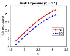
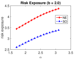
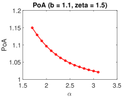
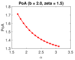
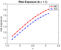
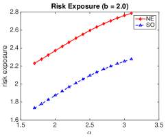
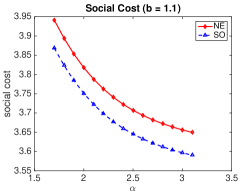
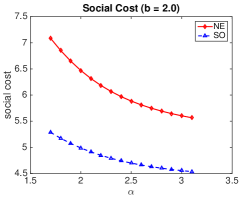
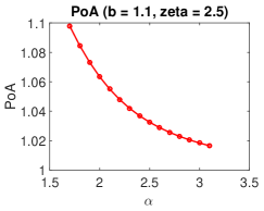
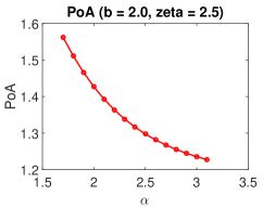
Fig. 1 plots the risk exposure and social cost at both NEs and social optima as well as the so-called price of anarchy (PoA) for $\zeta=1.5$ as we vary the value of power law parameter $\alpha$. The PoA is defined to be the ratio of the social cost at the worst NE to the minimum achievable social cost, and is a popular measure of the inefficiency of NE. Lemma 2 tells us that as $\alpha$ increases, the weighted degree distribution ${\bf w}$ becomes stochastically smaller. Thus, Theorems 3 and 4 state that the risk exposure rises at both NEs and social optima. This is confirmed by Fig. 1(a).

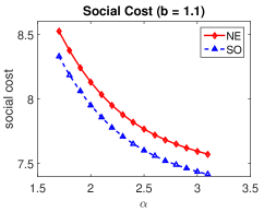
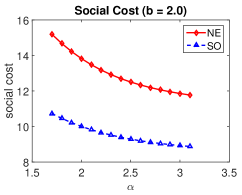
Our analytical findings, however, do not suggest how the social cost would behave with increasing $\alpha$. Fig. 1(b) shows that the social cost in fact decreases with $\alpha$ in spite of increasing risk exposure. This is because the underlying dependence graph becomes less connected and nodes have smaller degrees.

In addition, Figs. 1(b) and 1(c) indicate that the gap between the NE and social optimum widens both in risk exposure and social cost as the risk exposure (i.e., $g^{+}$) becomes more sensitive to the security investments when $b$ is raised to 2.0 from 1.1, thereby causing higher PoA. This observation is intuitive; when the risk exposure is more sensitive to security investments, when agents make less security investments at the NE compared to the social optimum, it leads to larger increase in risk exposure and social cost.

Finally, Fig. 1(c) illustrates that the PoA is larger when the dependence graph is more densely connected. This observation is consistent with that of [25]: Theorem 7 of [25] proves a tight upper bound on PoA, which is an affine function of the average node degree. Thus, as the dependence graph becomes more connected, leading to a higher average node degree, the NE becomes less efficient in that the PoA escalates.

(a)

(b)

(c)

Figure 2: (a) Risk exposure, (b) social cost and (c) price of anarchy ($\zeta=2.5$).

In order to examine how the infection probability function $p$ influences the risk exposure and social cost, we plot them for $\zeta=2.5$ (with the remaining parameters being identical as before) in Fig. 2. This represents a scenario in which the available security measures are more effective in that the infection probability falls more quickly with increasing security investments.

Comparing Figs. 1 and 2, we observe that although the final risk exposure and social costs are smaller than in the previous case with $\zeta=1.5$, their qualitative behavior remains similar. This indicates that as the security measures improve, both the risk exposure and the social cost will likely drop. However, we suspect that the properties of underlying dependence graph will have comparable effects on them.

VIII Conclusions

We examined how we could internalize the externalities produced by security investments of selfish agents in IDS settings. Our study brought to light an interesting relation between the local minimizers of social cost and the pure-strategy NEs of a related population game in which the costs of agents are modified to reflect their contributions to social cost. Making use of this relation, we demonstrated that it is possible to reduce the social cost and enhance the security by imposing appropriate penalties on the agents on the basis of the losses they suffer as a result of indirect attacks from their neighbors. Finally, we proved that as the security of agents becomes more interdependent and the weighted node degree distribution becomes stochastically larger, the local security experienced by a node with a fixed degree improves.

Appendix A Proof of Lemma 1

Let $H:{\mathcal{A}}^{D_{\max}}\to{\mathcal{A}}^{D_{\max}}$, where $H_{d}({\bf a})=I^{{\rm opt}}(\tau_{A}+d\cdot e({\bf a};{\bf s}))$, $d\in{\mathcal{D}}$. Then, from Assumption 1 and the definition of $I^{{\rm opt}}$, the mapping $H$ is continuous. Therefore, since ${\mathcal{A}}^{D_{\max}}$ is a compact, convex subset of ${\rm I\kern-2.5ptR}^{D_{\max}}$, the Brouwer’s fixed point theorem tells us that there exists a fixed point of $H$, say ${\bf a}^{\prime}$, such that $H({\bf a}^{\prime})={\bf a}^{\prime}$. It is clear from the definition of a pure-strategy NE in Definition 1 that ${\bf a}^{\prime}$ is a pure-strategy NE.

Appendix B Proof of Theorem 1

Before we proceed with the proof of theorem, recall that $e({\bf a};{\bf s})=g(\gamma_{{\rm avg}}({\bf a};{\bf s}))=g^{+}(\rho({\bf a};{\bf s}))$, where $\gamma_{{\rm avg}}({\bf a};{\bf s})=\tau_{A}\ \beta_{IA}\ {\bf w}({\bf s})^{T}{\bf p}({\bf a})=\tau_{A}\ \beta_{IA}\ \rho({\bf a};{\bf s})$ and $\rho({\bf a};{\bf s})={\bf w}({\bf s})^{T}{\bf p}({\bf a})$.

In order to prove the theorem, we will first show that if ${\bf a}^{1}$ and ${\bf a}^{2}$ are two pure-strategy NEs, then $e({\bf a}^{1};{\bf s})=e({\bf a}^{2};{\bf s})$. We will prove this claim by contradiction. Suppose that the claim is false and the risk exposures are not the same. Without loss of generality, assume $e({\bf a}^{1};{\bf s})<e({\bf a}^{2};{\bf s})$. Together with Corollary 1, this implies $p(a^{1}_{d})\geq p(a^{2}_{d})$ for all $d\in{\mathcal{D}}$ and, consequently,

$$e({\bf a}^{1};{\bf s}) = g^{+}\big{(}{\bf w}({\bf s})^{T}{\bf p}({\bf a}^{1})\big{)}$$

$$\geq g^{+}\big{(}{\bf w}({\bf s})^{T}{\bf p}({\bf a}^{2})\big{)}=e({\bf a}^{2};{\bf s}),$$

which contradicts the earlier assumption $e({\bf a}^{1};{\bf s})<e({\bf a}^{2};{\bf s})$.

The theorem is now a direct consequence of this claim and Corollary 1; if the theorem is false and there exist two distinct pure-strategy NEs ${\bf a}^{1}$ and ${\bf a}^{2}$, it necessarily implies that there is some $d^{\prime}\in{\mathcal{D}}$ such that $a^{1}_{d^{\prime}}<a^{2}_{d^{\prime}}$. However, this is possible only if $e({\bf a}^{1};{\bf s})<e({\bf a}^{2};{\bf s})$ by Corollary 1, which contradicts the claim proved above.

Appendix C Proof of Theorem 2

First, a local minimizer of social cost, say ${\bf a}^{\star}$, must satisfy the first-order necessary Karush-Kuhn-Tucker (KKT) condition [6]: There exist non-negative KKT multipliers $\boldsymbol{\lambda}=(\lambda_{d};\ d\in{\mathcal{D}})$ and $\boldsymbol{\mu}=(\mu_{d};\ d\in{\mathcal{D}})$ such that, for all $d\in{\mathcal{D}}$,

1. $\frac{\partial}{\partial a_{d}}\tilde{C}_{T}({\bf a}^{\star},{\bf s})=\lambda_{d}-\mu_{d}$, and

2. $\lambda_{d}(a^{\star}_{d}-I_{\min})=0$ and $\mu_{d}(I_{\max}-a^{\star}_{d})=0$.

From (8) and (9),

$$\frac{\partial}{\partial a_{d}}\tilde{C}_{T}({\bf a}^{\star},{\bf s})=\sum_{d^{\prime}\in{\mathcal{D}}}\frac{\partial}{\partial a_{d}}\tilde{C}({\bf a}^{\star},d^{\prime},{\bf s})$$

$$= \frac{\partial}{\partial a_{d}}e({\bf a}^{\star};{\bf s})\sum_{d^{\prime}\in{\mathcal{D}}}s_{d^{\prime}}\ d^{\prime}\ L(a^{\star}_{d^{\prime}})$$

$$+s_{d}\left(\big{(}\tau_{A}+d\ e({\bf a}^{\star};{\bf s})\big{)}L\ \dot{p}(a^{\star}_{d})+1\right),$$

where

$$\frac{\partial}{\partial a_{d}}e({\bf a}^{\star};{\bf s}) = \dot{g}^{+}\big{(}{\bf w}({\bf s})^{T}{\bf p}({\bf a}^{\star})\big{)}\ w_{d}({\bf s})\ \dot{p}(a^{\star}_{d})$$

$$= \dot{g}^{+}(\rho({\bf a}^{\star};{\bf s}))\ w_{d}({\bf s})\ \dot{p}(a^{\star}_{d}).$$

Substituting $w_{d}({\bf s})=d\cdot s_{d}/d_{{\rm avg}}({\bf s})$ and using $e({\bf a};{\bf s})=g^{+}\big{(}\rho({\bf a};{\bf s})\big{)}$ in the KKT conditions, we obtain

$$\frac{\partial}{\partial a_{d}}\tilde{C}_{T}({\bf a}^{\star},{\bf s})$$ (13)

$$= s_{d}\ d\ \dot{g}^{+}(\rho({\bf a}^{\star};{\bf s}))\ \rho({\bf a}^{\star};{\bf s})\ L\ \dot{p}(a^{\star}_{d})$$

$$+s_{d}\big{(}(\tau_{A}+d\ e({\bf a}^{\star};{\bf s}))L\ \dot{p}(a^{\star}_{d})+1\big{)}$$

$$= s_{d}\big{(}\big{(}\tau_{A}+d\ \vartheta(\rho({\bf a}^{\star};{\bf s}))\big{)}L\ \dot{p}(a^{\star}_{d})+1\big{)}$$

$$= \lambda_{d}-\mu_{d}.$$

Dividing both sides by $s_{d}$ yields

$$\big{(}\tau_{A}+d\ \vartheta(\rho({\bf a}^{\star};{\bf s}))\big{)}L\ \dot{p}(a^{\star}_{d})+1 = \frac{\lambda_{d}-\mu_{d}}{s_{d}}$$ (14)

$$= \lambda^{n}_{d}-\mu_{d}^{n},$$

where $\lambda^{n}_{d}=\lambda_{d}/s_{d}$ and $\mu^{n}_{d}=\mu_{d}/s_{d}$.

At a pure-strategy NE of the modified population game, ${{\bf a}}^{mc}$, a player in population $d$ faces the constrained convex optimization problem

$$\min_{a\in{\mathcal{A}}}\big{(}\tau_{A}+d\ \vartheta(\rho({{\bf a}}^{mc};{\bf s}))\big{)}L(a)+a.$$

From the definition of NE, the first-order necessary and sufficient KKT condition states that there exist non-negative KKT multipliers $\tilde{\lambda}_{d}$ and $\tilde{\mu}_{d}$ such that

$$\big{(}\tau_{A}+d\ \vartheta(\rho({\bf a}^{mc};{\bf s}))\big{)}L\ \dot{p}({a}^{mc}_{d})+1 = \tilde{\lambda}_{d}-\tilde{\mu}_{d}.$$ (15)

By comparing (14) and (15), we see that the local minimizer ${\bf a}^{\star}$, which satisfies the first-order necessary KKT conditions in (14), also meets the sufficient conditions in (15) with $\tilde{\lambda}_{d}=\lambda^{n}_{d}$ and $\tilde{\mu}_{d}=\mu^{n}_{d}$ for all $d\in{\mathcal{D}}$. Therefore, it is a pure-strategy NE of the modified population game.

Appendix D Proof of Theorem 3

Suppose that the first part of the theorem is false and $e({\bf a}^{1};{\bf s}^{1})>e({\bf a}^{2};{\bf s}^{2})$. By Corollary 1, this implies that, for all $d\in{\mathcal{D}}$,

$$p(a^{1}_{d})\leq p(a^{2}_{d}).$$ (16)

Using $e({\bf a};{\bf s})=g^{+}\big{(}{\bf w}({\bf s})^{T}{\bf p}({\bf a})\big{)}$ defined in Section III-A,

$$e({\bf a}^{2};{\bf s}^{2}) = g^{+}\big{(}{\bf w}({\bf s}^{2})^{T}{\bf p}(a^{2}_{d})\big{)}$$ (17)

$$\geq g^{+}\big{(}{\bf w}({\bf s}^{2})^{T}{\bf p}(a^{1}_{d})\big{)}$$

$$\geq g^{+}\big{(}{\bf w}({\bf s}^{1})^{T}{\bf p}(a^{1}_{d})\big{)}$$

$$= e({\bf a}^{1};{\bf s}^{1}),$$

which contradicts the earlier assumption. The first inequality in (17) follows from (16), and the second inequality in (D) is a consequence of the condition (11) in Theorem 3 and Corollary 1, i.e., $p(a^{i}_{d})\leq p(a^{i}_{d^{\prime}})$ if $d\geq d^{\prime}$, $i=1,2$.

The claim $a^{1}_{d}\leq a^{2}_{d}$ for all $d\in{\mathcal{D}}$ is an immediate consequence of the first part and Corollary 1, which states that the optimal investment is nondecreasing in the risk exposure seen by the players.

The second part of the theorem is true because, under the stated assumptions that ${\bf w}({\bf s}^{1})$ first-order stochastically dominates ${\bf w}({\bf s}^{2})$ and ${\bf a}^{2}\in$ int(${\mathcal{A}}^{D_{\max}}$), the inequality (D) is strict as a consequence of (the strict inequality in) Corollary 1.

Appendix E Proof of Theorem 4

We prove the first part of the theorem by contradiction. Suppose that the claim is false and $e({\bf a}^{\star}({\bf s}^{1});{\bf s}^{1})>e({\bf a}^{\star}({\bf s}^{2});{\bf s}^{2})$. First, note that Corollary 3 tells us that ${\bf a}^{\star}({\bf s}^{i})$, $i=1,2$, are the unique pure-strategy NE of the modified population games, and $a^{\star}_{d}({\bf s}^{i})\leq a^{\star}_{d+1}({\bf s}^{i})$ for all $d=1,\ldots,D_{\max}-1$. Together with this observation, the condition (11) in the theorem tells us that if $a^{\star}_{d}({\bf s}^{1})\geq a^{\star}_{d}({\bf s}^{2})$ for all $d\in{\mathcal{D}}$, then $\rho({\bf a}^{\star}({\bf s}^{1});{\bf s}^{1})\leq\rho({\bf a}^{\star}({\bf s}^{2});{\bf s}^{2})$. Consequently, $e({\bf a}^{\star}({\bf s}^{1});{\bf s}^{1})\leq e({\bf a}^{\star}({\bf s}^{2});{\bf s}^{2})$, thereby contradicting the assumption $e({\bf a}^{\star}({\bf s}^{1});{\bf s}^{1})>e({\bf a}^{\star}({\bf s}^{2});{\bf s}^{2})$. Therefore, there must exist some $d^{*}\in{\mathcal{D}}$ such that

$$a^{\star}_{d^{*}}({\bf s}^{1})<a^{\star}_{d^{*}}({\bf s}^{2}).$$ (19)

We will show that this contradicts the assumption that ${\bf a}^{\star}({\bf s}^{1})$ minimizes the social cost. For notational simplicity, we denote ${\bf a}^{\star}({\bf s}^{i})$, $i=1,2$, by ${\bf a}^{i}$ throughout the proof.

The first-order necessary KKT conditions tell us that there exist non-negative KKT multipliers $\boldsymbol{\lambda}^{i}=(\lambda^{i}_{d};d\in{\mathcal{D}})$ and $\boldsymbol{\mu}^{i}=(\mu^{i}_{d};d\in{\mathcal{D}})$, $i=1,2$, which satisfy

$$\lambda^{i}_{d}(a_{d}^{i}-I_{\min})=0,\ \mu^{i}_{d}(I_{\max}-a^{i}_{d})=0,\mbox{ and }$$

$$\frac{\partial}{\partial a_{d}}\tilde{C}_{T}({\bf a}^{i},{\bf s}^{i})=\lambda^{i}_{d}-\mu^{i}_{d},\ \mbox{for all }d\in{\mathcal{D}}.$$ (20)

Recall from (13) in Appendix C,

$$\frac{\partial}{\partial a_{d^{*}}}\tilde{C}_{T}({\bf a}^{1},{\bf s}^{1})$$ (21)

$$= s^{1}_{d^{*}}\big{(}\big{(}\tau_{A}+d^{*}\ \vartheta(\rho({\bf a}^{1};{\bf s}^{1}))\big{)}L\ \dot{p}(a^{1}_{d^{*}})+1\big{)}$$

$$= \lambda^{1}_{d^{*}}-\mu^{1}_{d^{*}}.$$

However, because $a^{1}_{d^{*}}<a^{2}_{d^{*}}\leq I_{\max}$, we have $\mu^{1}_{d^{*}}=0$. Setting $\mu^{1}_{d^{*}}=0$ and dividing both sides of (21) by $s^{1}_{d^{*}}$, we get

$$\big{(}\big{(}\tau_{A}+d^{*}\ \vartheta(\rho({\bf a}^{1};{\bf s}^{1}))\big{)}L\ \dot{p}(a^{1}_{d^{*}})+1\big{)}=\frac{\lambda^{1}_{d^{*}}}{s^{1}_{d^{*}}}\geq 0.$$ (22)

Similarly, since $a^{2}_{d^{*}}>a^{1}_{d^{*}}\geq 0$, we have $\lambda^{2}_{d^{*}}=0$ and

$$\frac{\partial}{\partial a_{d^{*}}}\tilde{C}_{T}({\bf a}^{2},{\bf s}^{2})$$

$$= s^{2}_{d^{*}}\big{(}\big{(}\tau_{A}+d^{*}\ \vartheta(\rho({\bf a}^{2};{\bf s}^{2}))\big{)}L\ \dot{p}(a^{2}_{d^{*}})+1\big{)}$$

$$= -\mu^{2}_{d^{*}}.$$

Normalizing both sides by $s^{2}_{d^{*}}$,

$$\big{(}\big{(}\tau_{A}+d^{*}\ \vartheta(\rho({\bf a}^{2};{\bf s}^{2}))\big{)}L\ \dot{p}(a^{2}_{d^{*}})+1\big{)}=\frac{-\mu^{2}_{d^{*}}}{s^{2}_{d^{*}}}\leq 0.$$ (23)

Recall that we assumed $e({\bf a}^{1};{\bf s}^{1})>e({\bf a}^{2};{\bf s}^{2})$, hence $\rho({\bf a}^{1};{\bf s}^{1})>\rho({\bf a}^{2};{\bf s}^{2})$. In addition, by Assumption 1, because $a^{1}_{d^{*}}<a^{2}_{d^{*}}$, we have $\dot{p}(a^{1}_{d^{*}})<\dot{p}(a^{2}_{d^{*}})<0$. Therefore, together with Assumption 4, we have

$$0\leq(\ref{eq:3-2})<(\ref{eq:3-3})\leq 0$$

which is a contradiction.

To prove the second part of the theorem, first note that the proof of the first part tells us ${\bf a}^{\star}({\bf s}^{1})\geq{\bf a}^{\star}({\bf s}^{2})$, where the inequality is elementwise. Second, under the stated assumption ${\bf a}^{\star}({\bf s}^{2})\in$ int(${\mathcal{A}}^{D_{\max}}$), Corollaries 1 and 3 imply $a^{\star}_{d}({\bf s}^{2})<a^{\star}_{d+1}({\bf s}^{2})$ for all $d=1,2,\ldots,D_{\max}-1$. Finally, together with these observations, the first-order stochastic dominance of ${\bf w}({\bf s}^{1})$ over ${\bf w}({\bf s}^{2})$ leads to $e({\bf a}^{\star}({\bf s}^{1});{\bf s}^{1})<e({\bf a}^{\star}({\bf s}^{2});{\bf s}^{2})$.

Appendix F Proof of Lemma 2

The following lemma will be used to prove Lemma 2.

Lemma 3

Suppose that ${\bf a}=(a_{\ell};\ell=1,\ldots,K)$ and ${\bf b}=(b_{\ell};\ell=1,\ldots,K)$ are two finite sequences of nonnegative real numbers of length $K>1$ and satisfy

$$\frac{b_{\ell+1}}{a_{\ell+1}}\leq\frac{b_{\ell}}{a_{\ell}}\ \mbox{ for all }\ell=1,\ldots,K-1.$$ (24)

Then,

$$\frac{\sum_{\ell=1}^{k}b_{\ell}}{\sum_{\ell=1}^{k}a_{\ell}} \geq \frac{\sum_{\ell=1}^{K}b_{\ell}}{\sum_{\ell=1}^{K}a_{\ell}}\ \mbox{ for all }k=1,\ldots,K.$$ (25)

Proceeding with the proof of Lemma 2, recall that the condition (12) in Lemma 2 states

$$\frac{(d+1)\ s^{2}_{d+1}}{(d+1)\ s^{1}_{d+1}} \leq \frac{d\cdot s_{d}^{2}}{d\cdot s_{d}^{1}}\ \mbox{ for all }d\in{\mathcal{D}}^{-}.$$ (26)

From the definition of ${\bf w}_{d}$, the condition (11) is equivalent to

$$\frac{\sum_{\ell=1}^{d}\ell\cdot s^{2}_{\ell}}{\sum_{\ell=1}^{d}\ell\cdot s^{1}_{\ell}} \geq \frac{\sum_{\ell=1}^{D_{\max}}\ell\cdot s_{\ell}^{2}}{\sum_{\ell=1}^{D_{\max}}\ell\cdot s_{\ell}^{1}}\ \mbox{ for all }d\in{\mathcal{D}}.$$ (27)

Let ${\bf a}=(a_{d};\ d\in{\mathcal{D}})$ and ${\bf b}=(b_{d};\ d\in{\mathcal{D}})$, where $a_{d}=d\cdot s^{1}_{d}$ and $b_{d}=d\cdot s^{2}_{d}$. The inequalities in (27) can be rewritten in terms of ${\bf a}$ and ${\bf b}$ as

$$\frac{\sum_{\ell=1}^{d}b_{\ell}}{\sum_{\ell=1}^{d}a_{\ell}} \geq \frac{\sum_{\ell=1}^{D_{\max}}b_{\ell}}{\sum_{\ell=1}^{D_{\max}}a_{\ell}}\ \mbox{ for all }d\in{\mathcal{D}}.$$ (28)

Moreover, (26) implies $(b_{d+1}/a_{d+1})\leq(b_{d}/a_{d})$, $d\in{\mathcal{D}}^{-}$. The claim of Lemma 2 in (28) now follows directly from Lemma 3.

References

- [1] National Vulnerability Database. http://nvd.nist.gov.
- [2] Introduction to NISTIR 7628 Guidelines for Smart Grid Cyber Security, Sep. 2010.
- [3] R. Anderson and T. Moore, “Information security economics - and beyond,” Lecture Notes in Computer Science Volume 4622, pp. 68-91, 2007.
- [4] Y. Baryshnikov, “IT security investment and Gordon-Loeb’s rule,” Proc. of the 11th Annual Workshop on the Economics of Information Security (WEIS), Berlin (Germany), Jun. 2012.
- [5] N. Beale, D.G. Rand, H. Battey, K. Croxson, R.M. May and M.A. Nowak, “Individual versus systemic risk and the regulator’s dilemma,” Proceedings of the National Academy of Sciences of the United States of America (PNAS), 108(31):12647-12652, Aug. 2011.
- [6] D.P. Bertsekas, Nonlinear Programming, Athena Scientific, 1995.
- [7] L. Bilge and T. Dumitras, “Before we knew it: an empirical study of zero-day attacks in the real world,” Proc. of ACM Conference on Computer and Communications Security (CCS), Oct. 2012.
- [8] J.C. Bolot and M. Lelarge, “A new perspective on Internet security using insurance,” Proc. of IEEE INFOCOM, Phoenix (AZ), Apr. 2008.
- [9] E. Bou-Harb, C. Fachkha, M. Pourzandi, M. Debbabi, and C. Assi, “Communication security for smart grid distribution networks,” IEEE Communications Magazine, pp. 42-49, Jan. 2013.
- [10] F. Caccioli, T.A. Catanach, and J.D. Farmer, “Heterogeneity, correlations and financial contagion,” arXiv:1109.1213, Sep. 2011.
- [11] F. Caccioli, T.A. Catanach, and J.D. Farmer, “Stability analysis of financial contagion due to overlapping portfolios,” arXiv:1210.5987, Oct. 2012.
- [12] D.S. Callaway, M.E.J. Newman, S.H. Strogatz and D.J. Watts, “Network robustness and fragility: percolation and random graphs,” Physical Review Letters, 85(25):5468-5471, Dec. 2000.
- [13] F. Chung and L. Lu, “Connected components in random graphs with given expected degree sequences,” Annals of Combinatorics, 6(2):125-145, Nov. 2002.
- [14] K.G. Gkonis and H.N. Psaraftis, “Container transportation as an interdependent security problem,” Journal of Transportation Security, 3(4):197-211, Dec. 2010.
- [15] J.P. Gleeson and D.J. Cahalane, “Seed size strongly affects cascades on random networks,” Phys. Rev. E, 75, 056103, 2007.
- [16] L.A. Gordon, M.P Loeb, W. Lucyshyn and L. Zhou, “Externalities and the magnitude of cyber security underinvestment by private sector firms: a modification of the Gordon-Loeb model,” Journal of Information Security, 6:24-30, 2015.
- [17] J. Grossklags, N. Christin and J. Chuang, “Secure or insecure? a game-theoretic analysis of information security games,” Proc. of of the 17th International Conference on World Wide Web, pp. 209-218, Beijing (China), Apr. 2008.
- [18] G. Heal, H.C. Kunreuther and P.R. Orszag, “Interdependent security: Implications for homeland security policy and other areas,” Brookings Policy Brief Series, #108, Oct. 2002.
- [19] G. Heal and H.C. Kunreuther, “Interdependent security: a general model,” National Bureau of Economic Research (NBER) Working Paper No. 10706, Aug. 2004.
- [20] A. Hofmann, “Internalizing externalities of loss prevention through insurance monopoly: an analysis of interdependent risks,” Geneva Risk Insurance Review, 32:91-111, 2007.
- [21] L. Jiang, V. Anantharam and J. Walrand, “How bad are selfish investments in network security?”, IEEE/ACM Transactions on Networking, 19(2):549-560, Apr. 2011.
- [22] M. Kearns and L.E. Ortiz, “Algorithms for interdependent security games,” Advances in Neural Information Processing Systems 16, 2003.
- [23] H.C. Kunreuther and G. Heal, “Interdependent Security,” The Journal of Risk and Uncertainty, 26(2/3):231-249, 2003.
- [24] H.C. Kunreuther and E.O. Michel-Kerjan, “Assessing, managing and benefiting from global interdependent risks: The case of terrorism and natural disasters,” Global Business and the Terrorist Threat, edited by H.W. Richardson, P. Gordon and J.E. Moore, Edward Elgar Publishing, 2009.
- [25] R.J. La, “Interdependent security with strategic agents and global cascade,” IEEE/ACM Trans. on Networking, 24(3):1378-1391, Jun. 2016.
- [26] R.J. La, “Influence of network mixing on interdependent security: local analysis,” under review. A preprint available at http://www.ece.umd.edu/hyongla/preprint/La_Globecom16_TR.pdf.
- [27] A. Laszka, M. Felegyhazi and L. Buttyn, “A survey of interdependent information security games,” ACM Computing Surveys, 47(2):23:1-23:38, Jan. 2015.
- [28] M. Lelarge and J. Bolot, “A local mean field analysis of security investments in networks,” Proc. of the 3rd International Workshop on Economics of Networked Systems (NetEcon), pp. 25-30, Seattle (WA), Aug. 2008.
- [29] M. Lelarge and J. Bolot, “Economic incentives to increase security in the Internet: the case for insurance,” Proc. of IEEE INFOCOM, Rio de Janeiro (Brazil), Apr. 2009.
- [30] R.A. Miura-Ko, B. Yolken, N. Bambos and J. Mitchell, “Security investment games of interdependent organizations,” Proc. of Annual Allerton Conference, pp. 252-260, Monticello (IL), Sep. 2008.
- [31] P. Naghizadeh and M. Liu, “Closing the price of anarchy gap in the interdependent security game,” Information Theory and Applications (ITA) Workshop, San Diego (CA), Feb. 2014.
- [32] M.E.J. Newman, “Assortative mixing in networks,” Phys. Rev. Lett., 89, 208701, Oct. 2002.
- [33] M.E.J. Newman, “Mixing patterns in networks,” Phys. Rev. E, 67, 026126, Feb. 2003.
- [34] H. Ogut, N. Menon and S. Raghunathan, “Cyber insurance and IT security investment: impact of interdependent risk,” Proc. of the 4th Workshop on the Economics of Information Security (WEIS), Cambridge (MA), Jun. 2005.
- [35] R. Pastor-Satorras and A. Vespignani, “Epidemics and immunization in scale-free networks,” Handbook of Graphs and Networks: From the Genome to the Internet, Wiley, 2005.
- [36] W.H. Sandholm Population Games and Evolutionary Dynamics, The MIT Press, 2010.
- [37] C.M. Schneider, M. Tamara, H. Shlomo, H.J. Herrmann, “Suppressing epidemics with a limited amount of immunization units,” Phys. Rev. E, 84, 061911, Dec. 2011.
- [38] M. Shaked and J.G. Shanthikumar, Stochastic Orders, Springer Series in Statistics, Springer, 2007.
- [39] C. Shapiro and H.R. Varian, Information Rules, Harvard Business School Press, 1999.
- [40] H.R. Varian, “System reliability and free riding,” Economics of Information Security, 12:1-15, 2004.
- [41] H.R. Varian, Microeconomic Analysis, 3rd edition, W.W. Norton & Company, 1992.
- [42] D.J. Watts, “A simple model of global cascades on random networks,” Proceedings of the National Academy of Sciences of the United States of America (PNAS), 99(9):5766-5771, Apr. 2002.
- [43] O. Yaan and V. Gligor, “Analysis of complex contagions in random multiplex networks,” Physical Review E, 86, 036103, Sep. 2012.
- [44] X. Zhao, L. Xue and A.B. Whinston, “Managing interdependent information security risks: cyberinsurance, managed security services, and risk pooling arrangements,” Proc. of International Conference on Information Systems (ICIS), Phoenix (AZ), 2009.