Finding Likely Errors with Bayesian Specifications

Abstract

We present a Bayesian framework for learning probabilistic specifications from large, unstructured code corpora, and a method to use this framework to statically detect anomalous, hence likely buggy, program behavior. The distinctive insight here is to build a statistical model that correlates all specifications hidden inside a corpus with the syntax and observed behavior of programs that implement these specifications. During the analysis of a particular program, this model is conditioned into a posterior distribution that prioritizes specifications that are relevant to this program. This allows accurate program analysis even if the corpus is highly heterogeneous. The problem of finding anomalies is now framed quantitatively, as a problem of computing a distance between a “reference distribution” over program behaviors that our model expects from the program, and the distribution over behaviors that the program actually produces.

We present a concrete embodiment of our framework that combines a topic model and a neural network model to learn specifications, and queries the learned models to compute anomaly scores. We evaluate this implementation on the task of detecting anomalous usage of Android APIs. Our encouraging experimental results show that the method can automatically discover subtle errors in Android applications in the wild, and has high precision and recall compared to competing probabilistic approaches.

1 Introduction

Over the years, research on automated bug finding in programs has had many real-world successes Bessey et al. , [2010]; Ball et al. , [2011]. However, one perennial source of difficulty here is the need for formal specifications. Traditional approaches in this area require the user to specify correctness properties; any property that is not specified is outside the scope of reasoning. However, formally specifying real-world software is a difficult task that users often refuse to undertake.

A natural response to this difficulty is to automatically learn specifications of popular software components like APIs and frameworks. The availability of large corpora of open-source code — Big Code Raychev et al. , [2015], in the language of some recent efforts — makes this idea especially appealing. By analyzing these corpora, one can generate numerous examples of how real-world programs use a set of components. Statistical methods can then be used to learn common patterns in these examples. According to the well-known thesis that bugs are anomalous behaviors Engler et al. , [2001]; Hangal & Lam, [2002], a program whose use of the components significantly deviates from these “typical” usage patterns can be flagged as erroneous.

The problem of specification learning has been studied for a long time Ammons et al. , [2002, 2003]; Alur et al. , [2005]; Goues & Weimer, [2009]. However, existing approaches to the problem face two basic issues when applied to large code corpora. First, examples derived from such a corpus can be noisy. While programs in a mature corpus are likely to be correct on the average, not all examples extracted from such a corpus represent correct behavior. Second, such a corpus is fundamentally heterogeneous, and may contain many different specifications, some of them mutually contradictory. For example, it may be legitimate to use a set of APIs in many different ways depending on the context, and a large enough corpus would contain instances of all these usage patterns. A specification learning tool should distinguish between these patterns, and a bug-finding tool should only compare a program with the patterns that are relevant to it.

Among existing methods for specification learning, the majority follow a traditional, qualitative view of program correctness. In this view, a specification is a set of program behaviors (e.g., sequences of calls to API methods), and a behavior is either correct (in the specification) or incorrect (outside the specification). Such an approach is not robust to noise because its belief in the correctness of a behavior does not change smoothly with the behavior’s observed frequency. A small number of incorrect examples can persuade the method that the behavior is fully correct.

An obvious fix to this problem is to view a specification as a probabilistic rather than a boolean model. Such a specification assigns quantitative likelihood values to observed program behaviors, with higher likelihood representing greater confidence in a behavior’s correctness. Some recent work adopts this view by modeling program behaviors using models like $n$-grams Nguyen & Nguyen, [2015]; Wang et al. , [2016a] and recurrent neural networks Raychev et al. , [2014]. To find bugs using such a model, one generates behaviors of the target program using static or dynamic analysis, then evaluates the likelihood of these behaviors Wang et al. , [2016b].

While robust to noise, approaches of this sort have a basic difficulty with heterogeneity. The root of this difficulty is that these methods learn a single probability distribution over program behaviors. For example, if $\Psi_{1}$ and $\Psi_{2}$ are two common but distinct patterns in which programs in a corpus use a set of APIs, these approaches would learn a specification that is a mixture of $\Psi_{1}$ and $\Psi_{2}$. During program analysis, such a mixture would assign low or meaningless likelihoods to behaviors that match one of, but not both, $\Psi_{1}$ and $\Psi_{2}$. As behaviors from a given program are likely to follow only one of the two patterns, this phenomenon would lead to inaccurate analysis.

In this paper, we present a Bayesian approach to specification learning and bug finding that is robust to heterogeneity and noise. Our key insight is to build a “big” statistical model that captures the entire gamut of specifications in an unstructured code corpus. More precisely, our model learns a joint probability distribution that relates hidden specifications $\Psi$ with syntactic features $X$ that describe what implementations of these specifications “look like”. When using this model to analyze a particular program $F$, we specialize it into a posterior distribution $P(\Psi|X_{F})$ over specifications, conditioned on the features $X_{F}$ of $F$. Intuitively, this distribution assigns higher weight to specifications for programs that “look like” $F$, and can be seen as the part of the model that is relevant to $F$.

This model architecture can tolerate high (in principle, unbounded) amounts of heterogeneity in the corpus. Suppose that the programs in the corpus use a set of APIs following distinct patterns $\Psi_{1},\dots,\Psi_{n}$, but that programs that look like $F$ (i.e., have feature set $X_{F}$) tend to follow $\Psi_{1}$. During training, our framework learns this correlation between $X_{F}$ and $\Psi_{1}$. This means that the posterior distribution $P(\Psi|X_{F})$ puts a high weight on $\Psi_{1}$ and low weights on $\Psi_{2},\dots,\Psi_{n}$, and that effectively, correctness analysis of $F$ happens with respect to $\Psi_{1}$ rather than any other specification.

Our second key idea is to frame the detection of likely errors as an operation over probability distributions. We assume, for each program $F$, a distribution $P_{F}(\theta)$ over the behaviors of the program. This distribution — a probabilistic behavior model — may be learned from data, or, as is the case in this paper, be a definition that is a parameter of the framework. This allows us to develop a model $P(\theta|\Psi)$ of the behaviors $\theta$ of a program that follows a specification $\Psi$. When combined with the posterior distribution $P(\Psi|X_{F})$ for $\Psi$, this model gives us a “reference distribution” $P(\theta|X_{F})$ over behaviors that the model expects from a program that looks like $F$. The anomaly score of $F$, which quantifies the extent to which $F$ behaves abnormally, is now defined as a statistical distance (in particular, the Kullback-Leibler divergence Kullback & Leibler, [1951]) between $P(\theta|X_{F})$ and $P_{F}(\theta)$.

Our Bayesian approach is a framework, meaning that it can be implemented using a wide range of concrete statistical models. The particular instantiation we present in this paper is a combination of the popular topic model known as Latent Dirichlet Allocation (LDA) Blei et al. , [2003], and a class of neural networks that are conditioned on a topic model Mikolov & Zweig, [2012]. To compute the anomaly score for a program $F$, we repeatedly query this model for the likelihood of different behaviors of $F$, and then aggregate these likelihood values into an estimate of the anomaly score.

We evaluate our implementation in the task of finding erroneous API usage in Android applications. Using three APIs as benchmarks, we show that the tool can automatically discover subtle API bugs in Android applications in the wild. These violations range from GUI bugs to inadequate encryption strength. Some of these errors are difficult to characterize in logic-based specification notations, indicating the promise of our approach in settings where traditional formal methods are hard to apply. We also demonstrate that the method has good precision recall and is more robust to heterogeneity than a comparable non-Bayesian approach.

Now we summarize the contributions of this paper:

• We present a novel Bayesian framework for learning specifications from large code corpora. (Section 3)

• We offer a novel formulation of the problem of finding anomalous program behavior as the problem of computing a distance between a program and a reference distribution. (Section 3)

• We present an instantiation our framework with a topic model and a topic-conditioned recurrent neural network. (Section 4)

• We evaluate the approach on the problem of detecting anomalous API usage in a suite of Android applications (Section 5)

2 Overview

In this section, we present an overview of our approach, with the help of an illustrative example.

2.1 Modeling Framework and Workflow

Our approach has the following key aspects. First, we assume the existence of a specification $\Psi$ for each program $F$. However, unlike traditional approaches that start with a formal specification, $\Psi$ in our context is not observable. Instead, what is observable is $X_{F}$, a set of syntactic features for $F$. The features are evidence, or data, that inform our opinion as to the unseen specification $\Psi$. In Bayesian fashion, our uncertainty about $\Psi$ is formalized as a posterior distribution $P(\Psi|X_{F})$, which measures the extent to which we believe that $\Psi$ is the correct specification for $F$, given the evidence.

Second, our framework allows for uncertainty regarding the behaviors $\theta$ — defined as sequences of observable actions — that a given program $F$ produces. This uncertainty comes from the fact that we do not exactly know the inputs on which the program will run, and is captured by a probability distribution $P_{F}(\theta)$. The framework also allows for a distribution $P(\theta|\Psi)$ over the behaviors of programs that implement a given specification $\Psi$. This uncertainty can come from the fact that we do not know the inputs to implementations of $\Psi$, or the fact that we may have never seen a specification exactly like $\Psi$ before, so that we have to guess the behavior of a program implementing $\Psi$.

Our a priori belief about the relationships between specifications and the features and behaviors of their implementations is given by a joint distribution $P(\theta,X_{F},\Psi)$. Our third key idea is that this distribution is informed by data extracted from a corpus of code. This information is taken into account formally during a learning phase that fits the joint distribution prior model to the data.

Finally, in the inference phase, we frame bug detection as a problem of computing a quantitative anomaly score. In traditional correctness analysis, the semantics of programs and specifications are given by sets, and one checks if the set difference between a program and a specification is empty. Our formulation is a quantitative generalization of this, and defines the anomaly score for a program $F$ as the Kullback-Leibler (KL) divergence Kullback & Leibler, [1951] between the behavior distribution $P_{F}(\theta)$ for $F$, and the posterior distribution $P(\theta|X_{F})$ that the model expects from $F$. Correctness analysis amounts to checking whether this score is below a threshold.

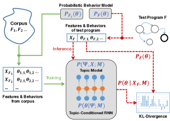
Figure 1: Workflow, with instantiations in grey boxes

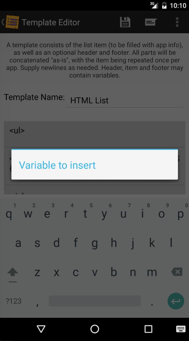
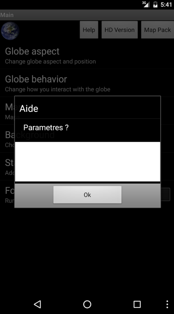
		⬇ 1AlertDialog.Builder b = new AlertDialog.Builder(this); 2b.setTitle(R.string.title_variable_to_insert); 3if (focus.getId() == R.id.tmpl_item) 4 b.setItems(R.array.templatebodyvars, this); 5else if (focus.getId() == R.id.tmpl_footer) 6 b.setItems(R.array.templateheaderfootervars, this); 7b.show(); (b)(i) ⬇ 1AlertDialog.Builder b = new AlertDialog.Builder(this); 2b.setMessage("Parametres?"); 3b.setCancelable(false); 4b.setView(dlgLayout); 5b.setPositiveButton("Ok", new OnClickListener(){$\ldots$}); 6b.setTitle("Aide") 7b.show();
(a)(i)	(a)(ii)	(b)(ii)

Figure 2: (a) Abnormal dialog boxes discovered by our anomaly detection (b) Code snippets corresponding to the dialog boxes

The workflow of our method is as in Figure 1. The training and inference phases are denoted by green (solid) edges and red (dashed) edges respectively. During training, from each program $F_{i}$ in a large corpus of programs $F_{1},F_{2},\dots$, we extract a set of syntactic features $X_{F_{i}}$, and sample a set of behaviors from the distribution $P_{F_{i}}(\theta)$, forming the training data. From this data, we learn the joint distribution $P(\theta,X,\Psi;\textbf{M})$, where M are the model parameters.

During inference, we extract the features $X_{F}$ of a given program $F$, and query the trained model for the distribution $P(\theta|X_{F};\textbf{M})$ that tells us how $F$ should behave. Separately, we obtain the distribution $P_{F}(\theta)$ over observed behaviors of $F$. The anomaly score of $F$ is then computed as the KL-divergence between these distributions.

2.2 Instantiating the Framework

An instantiation of our framework must concretely define program features and behaviors, and the way in which the distributions $P(\theta,X,\Psi;\textbf{M})$ and $P_{F}(\theta)$ are obtained. In this paper, we consider a particular instantiation where the goal is to learn patterns in the way programs call methods in a set of APIs. We abstract each such call as a symbol from a finite set, and define a behavior $\theta$ as a sequence of symbols. The feature $X_{F}$ for a program $F$ is the set of symbols that $F$ can generate.

A key idea in the instantiation is to capture hidden specifications using a topic model. Here, “topic” is an abstraction of the hidden semantic structure of a program. A specification for a program $F$ is a vector of probabilities whose the $i$-th component is the probability that $F$ follows the $i$-th topic. For example, the topics in a given corpus may correspond to GUI programs and bit-manipulating programs. A program that makes many calls to GUI APIs will likely have a higher probability for the former topic.

Specifically, we use the well-known Latent Dirichlet Allocation (LDA) Blei et al. , [2003] topic model to learn a joint distribution $P(\Psi,X;\textbf{M})$ over the topics and features of programs. A topic-conditioned recurrent neural network model Mikolov & Zweig, [2012], is used to as the second model $P(\theta|\Psi;\textbf{M})$. The joint distribution $P(\theta,X,\Psi;\textbf{M})$ that our framework maintains can be factored into these two distributions.

Our probabilistic model $P_{F}(\theta)$ for behaviors of programs $F$ is not data-driven. This is because to learn this distribution statistically, we would need data on the inputs that $F$ receives in the real world. Since such data is not available in typical code corpora, we simply assume a definition of $P_{F}(\theta)$. While many such definitions are possible, the one we pick models $F$ as a class of automata, called generative probabilistic automata Ammons et al. , [2002]; Murawski & Ouaknine, [2005]. The distribution $P_{F}(\theta)$ is simply the semantics of this automaton.

2.3 Example

Consider the problem of finding bugs in GUIs, where the right and wrong ways of invoking GUI API methods are seldom formally defined. Specifically, consider a dialog box in a GUI that does not give the user an option to close the box, and a dialog box that does not display any textual content. Clearly, such boxes violate user expectations, and are buggy in that sense. Two such boxes, produced by real-world Android apps, are shown in Figure 2(a).

The code snippets responsible for these boxes are shown in Figure 2. For example, in Figure 2(b)(i), ${\tt b}$ is a dialog box; the method ${\tt b.setItems(...)}$ adds content to the dialog box; the method ${\tt b.show()}$ displays the box. If the branches in lines 4 and 7 are not taken, then ${\tt b.show()}$ opens the box without a “close” button. Note that the sequences of API calls that lead to these bugs are not forbidden by the API, and would not be caught by a traditional program analysis. In contrast, a statistical method like ours can observe thousands of programs and learn that these sequences are abnormal.

Operationally, to debug this program, we generated features and behaviors from a corpus of Android apps. Using these features, LDA learned to classify programs by the APIs they use, and to also distinguish between different usage patterns in the same API. Consider the examples of dialog box creation in Figure 2(b), where program $F_{1}$ in (b)(i) explicitly specifies the items that go into the box, and the program $F_{2}$ in (b)(ii) provides a ${\tt View}$ that encompasses the items that go into the box. LDA can assign different topics to these usage patterns. For example, the pattern used in $F_{1}$ could be assigned the first topic, resulting in a topic vector ($\Psi$) $\langle 0.98,0.01,0.01\rangle$, and the pattern used in $F_{2}$ could be assigned the second topic, resulting in the topic vector $\langle 0.01,0.98,0.01\rangle$.

Conditioned on such a topic vector $\Psi$, a topic-conditioned RNN provides the probability of an API call sequence $\theta$, that is, $P(\theta|\Psi)$. For instance, given the former topic vector, a topic-conditioned RNN trained on thousands of examples of topics and behaviors would provide a high probability to a sequence such as:

${\tt new~{}A()~{}~{}setTitle(...)~{}~{}setItems(...)~{}~{}show()}$

(where ${\tt new~{}A()}$ is a call to the constructor) and a low probability to an abnormal sequence such as

${\tt new~{}A()~{}~{}setTitle(...)~{}~{}show()}$

as it shows a dialog without any content. However, our probabilistic automaton model $P_{F_{1}}(\theta)$ of $F_{1}$ would assign about 0.66 and 0.33 probability, respectively, to these sequences. In general, the KL-divergence between the two distributions will be high, causing $F_{1}$ to be flagged as anomalous.

3 Bayesian Specification Framework

In this section, we formalize our framework, along with the problems of specification learning and anomaly detection.

3.1 Program Behaviors and Features

Our framework is parameterized by a programming language. Each program in the language has a syntax and an operational semantics. Because the details of the language do not matter to the framework, we do not concretely define this syntax and semantics. Instead, we assume that the syntax of each program $F$ can be abstracted into a feature set $X_{F}$. For instance, such features can include syntactic constructs, assertions, and natural language comments. We also assume that program actions during execution can be abstracted into a finite alphabet $\Sigma$ of observable symbols (including an empty symbol $\epsilon$). We model program executions as behaviors $\theta$, defined to be words in $\Sigma^{*}$. A behavior is the result of a probabilistic generative process that takes place when a program is executed. Accordingly, we assume a probabilistic behavior model of $F$, defined as a distribution $P_{F}(\theta)$ over the behaviors of $F$.

3.2 Specification Learning

Our Bayesian statistical framework builds a generative model of the form $P(\theta,X,\Psi)=P(\theta|\Psi)P(X|\Psi)P(\Psi)$. This model captures the intuition that every program is implementing some unknown specification in the space of all specifications ($P(\Psi)$), which determines the program’s behavior ($P(\theta|\Psi)$) and features ($P(X|\Psi)$).

Building this model requires data, in the form of a large corpus of example programs. As in all statistical learning methods, we first develop an appropriate statistical model, which is typically a distribution family, and then learn that model—choose the parameters for the model family so they match reality—by training it on data. To this end, $P(\theta,X,\Psi)$ also takes as input a set of model parameters M. Fully parameterized, this distribution becomes:

$$P(\theta,X,\Psi;\textbf{M})=P(\theta|\Psi;\textbf{M})P(X|\Psi;\textbf{M})P(\Psi;\textbf{M})$$ (1)

The available data are then used to choose an appropriate set of parameters M, using an optimization method such as maximum likelihood. Suppose that we are given a large corpus of programs $\{F_{1},\ldots,F_{N}\}$, and for each program $F_{i}$ we have extracted the pair $(X_{F_{i}},\langle\theta_{i,1}~{}\theta_{i,2},\ldots\rangle)$ consisting of its feature set and a number of examples of its behavior sampled from its behavior model. Given this data, we would choose M that maximizes the function:

$$\prod_{i=1}^{N}\left(\int_{\Psi}\left(\prod_{\theta_{i,j}}P(\theta_{i,j}|\Psi;\textbf{M})\right)P(X_{F_{i}}|\Psi;\textbf{M})P(\Psi;\textbf{M})~{}~{}d\Psi\right)$$

Note that we integrate out $\Psi$, since this is an unseen random variable, as we typically do not know the value of the precise specification associated with each code in the corpus. Once M is learned, the distribution would represent our prior belief as to what the “typical” specification, behavior and features look like, informed by the programs in the corpus.

3.3 Anomaly Detection

Suppose that we are given a new program $F$ and would like to obtain a quantitative measure of the “bugginess” of $F$. On the one hand, since we already have learned a joint distribution over behaviors, features and specifications, $P(\theta,X,\Psi;\textbf{M})$, we can condition this distribution with the newly observed $X_{F}$, to obtain the posterior:

$$P(\theta,\Psi|X_{F};\textbf{M})=\frac{P(\theta,\Psi,X_{F};\textbf{M})}{P(X_{F};\textbf{M})}$$

From Equation 1, we have

$$P(\theta,\Psi|X_{F};\textbf{M})=\frac{P(\theta|\Psi;\textbf{M})P(X_{F}|\Psi;\textbf{M})P(\Psi;\textbf{M})}{P(X_{F};\textbf{M})}$$

Applying Bayes’ rule to the term $P(X_{F}|\Psi;\textbf{M})$ we get $P(\theta,\Psi|X_{F};\textbf{M})$

$$=\frac{P(\theta|\Psi;\textbf{M})\displaystyle{\frac{P(\Psi|X_{F};\textbf{M})P(X_{F};\textbf{M})}{P(\Psi;\textbf{M})}}P(\Psi;\textbf{M})}{P(X_{F};\textbf{M})}$$

$$=P(\theta|\Psi;\textbf{M})P(\Psi|X_{F};\textbf{M})$$

From this, since we do not know the precise specification that $F$ is implementing, we can integrate out $\Psi$ to obtain the (marginalized) posterior distribution over behaviors:

$$P(\theta|X_{F};\textbf{M})=\int_{\Psi}P(\theta|\Psi;\textbf{M})P(\Psi|X_{F};\textbf{M})~{}d\Psi$$ (2)

This particular form is very amenable to Monte Carlo integration, which estimates an integral through random sampling. Intuitively, it gives us a distribution over the program behaviors $\theta$, that would be anticipated, given learned model parameters M, for a program with feature set $X_{F}$.

On the other hand, we have a distribution $P_{F}(\theta)$ over the actual behaviors of $F$ when it is executed. The final step is to then compare this actual distribution with the anticipated distribution over behaviors, that is, $P_{F}(\theta)$ and $P(\theta|X_{F};\textbf{M})$. A measure such as the Kullback-Leibler (KL) divergence Kullback & Leibler, [1951] between distributions is appropriate here. The KL-divergence between two distributions $P_{1}$ and $P_{2}$ over the domain $i$ is a quantitative measure defined as:

$$\mbox{$D_{KL}(P\|Q)$}=\sum_{i}P_{1}(i)\log\frac{P_{1}(i)}{P_{2}(i)}$$ (3)

Using this measure, we can compute the anomaly score of $F$ by setting $P_{1}$ and $P_{2}$ to the distributions $P_{F}(\theta)$ and $P(\theta|X_{F};\textbf{M})$ respectively, and ranging $i$ over the domain of all possible program behaviors in the language $\Sigma^{*}$:

$$\sum_{\theta\in\Sigma^{*}}P_{F}(\theta)\log\displaystyle{\frac{P_{F}(\theta)}{P(\theta|X_{F};\textbf{M})}}$$ (4)

Choosing an Abstraction

When instantiating the framework, the exact form of the feature set $X_{F}$ must be chosen with some care. If the feature set $X_{F}$ does not provide any abstraction for the program (in the extreme case, $X_{F}$ is merely the program itself) and the model and learner are arbitrarily powerful, then $P(\theta|X_{F};\textbf{M})$ (Equation 2) could, in theory, describe the compiler and symbolic executor used to produce the training data. This would mean that the KL divergence (Equation 3) is zero for any program.

When applying the framework to a problem, we protect against this possibility by choosing a feature set $X_{F}$ that abstracts the program to an appropriate level for the debugging task. For example, when debugging API usage, it makes sense to choose $X_{F}$ as the bag of API calls made by the code. This ensures that $P(\theta|X_{F};\textbf{M})$ is limited to attaching probabilities to various sequences that can be made out of those calls, and it is impossible for the learner to “learn” to compile and execute a program.

4 Instantiation of the Framework

In this section, we present an instantiation of our framework, and discuss practical implementation challenges.

4.1 Probabilistic Behavior Model $P_{F}(\theta)$

First, our instantiation includes a definition of the probabilistic behavior model $P_{F}(\theta)$. This definition relies on the abstraction of programs as generative probabilistic automata Murawski & Ouaknine, [2005]; Sokolova & de Vink, [2004].

Program Model.

A generative probabilistic automaton is a tuple $F=\langle\mathcal{Q},\Sigma,q_{0},Q_{A},\delta\rangle$ where $\mathcal{Q}$ is a finite set of states, $\Sigma$ is the alphabet of observable symbols that was introduced earlier, $q_{0}\in\mathcal{Q}$ is the initial state, $Q_{A}\subseteq\mathcal{Q}$ is a set of final or accepting states, and $\delta:\mathcal{Q}\times\Sigma\times\mathbb{R}_{(0,1]}\times\mathcal{Q}$ is a transition relation. We have $\delta(q_{i},s,p,q_{j})$ if the automaton can transition between states $q_{i}$ and $q_{j}$ with a probability $p\in(0,1]$, generating the symbol $s$. (We write $q_{i}~{}\xrightarrow{s,p}~{}q_{j}$ if such a transition exists.) Transitions with probability 0, or infeasible transitions, are excluded from the automaton.

A program in a high-level language is transformed into the above representation through symbolic execution King, [1976], during a preprocessing phase. Symbolic execution runs a program with symbolic inputs and keeps track of symbolic states, which are analogous to a program’s memory. The symbolic states encountered become the states $\mathcal{Q}$, and the accepting states $Q_{A}$ are typically the states at a final location (or some location of interest) in the program. Unbounded loops can be handled by imposing a bound on symbolic loop unrolls, or through a predicate abstraction of the program to make variable domains finite. The detection of infeasible states—in general an undecidable problem—depends on the underlying theorem prover used by symbolic execution.

As symbolic execution is a standard method in formal methods Jaffar et al. , [2012]; Cadar et al. , [2008]; Anand et al. , [2007], this section only gives an example of the method’s use. As it is applied at a preprocessing level, we often use the term “program” to refer to an automaton generated via symbolic execution, rather than a higher-level program to which preprocessing is applied.

Semantics.

A run $\pi$ of $F$ is defined as a finite sequence of transitions $q_{0}~{}\xrightarrow{s_{1},p_{1}}~{}q_{1}~{}\xrightarrow{s_{2},p_{2}}~{}\cdots~{}\xrightarrow{s_{n},p_{n}}~{}q_{n}$ beginning at the initial state $q_{0}$. $\pi$ is accepting if $q_{n}\in Q_{A}$. The probability of a run $P(\pi)=\prod_{i=1}^{n}p_{i}$. Every run $\pi$ generates a behavior $\theta\in\Sigma^{*}$, denoted as $[|\pi|]=s_{1}s_{2}\cdots s_{n}$. Let $\Pi_{F}$ be the set of all accepting runs of $F$, and $\Pi_{F}(\theta)\subseteq\Pi_{F}$ be the set of all accepting runs $\pi$ such that $[|\pi|]=\theta$. The probabilistic behavior model $P_{F}(\theta):\Sigma^{*}\rightarrow[0,1]$ is:

$$P_{F}(\theta)=\displaystyle{\frac{1}{Z}}\sum_{\pi\in\Pi_{F}(\theta)}P(\pi).$$ (5)

Here, $Z=\sum_{\pi\in\Pi_{F}}P(\pi)$ is a normalization factor.

It is easy to see that $P_{F}(\theta)$ defines a probability distribution over behaviors. To generate a “random” behavior of $F$, we simply sample from the distribution $P_{F}(\theta)$.

Features.

Given a program $F$, the feature set $X_{F}$ is defined as $\{s~{}|~{}q_{i}~{}\xrightarrow{s,p}~{}q_{j}\in\delta\}\setminus\{\epsilon\}$, i.e., the set of all non-empty symbols in the transition system of $F$.

Example.

The automaton model for the code in Figure 2(b)(i) is shown in Figure 3. Each “state” in the automaton is labeled with a program location, with multiple instances of the same location being primed. The initial state is the first location, and the accepting states, in bold, are all instances of a (special) terminal location $T$ in the program. The transitions follow the structure of the code (for brevity, we collapse sequential statements into a single transition), emitting as symbols API methods called at each location.

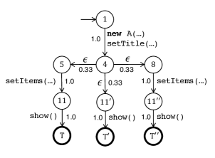
Figure 3: Automaton for the example in Figure 2(b)(i)

Note that we gave a uniform probability at each state to transition to the next possible states, but this can be controlled through other means. For instance, one can apply model counting on a branch condition and compute the probability of the program executing one branch over another. Such a definition is not necessarily a better choice than ours, as it would assign low probabilities to corner cases that get triggered on a small number of inputs but are often of interest to users of static analysis. The two definitions simply make different tradeoffs. We go with a uniform distribution at branches because it is simpler and worked well in our experiments.

$\{{\tt new~{}A()},{\tt setTitle(\ldots)},$ ${\tt setItems(\ldots)},{\tt show()}\}$ is the feature set for this program. There are three accepting runs of $F$, and two behaviors generated by these accepting runs:

$\theta_{1}={\tt new~{}A()}~{}~{}{\tt setTitle(\ldots)}~{}~{}{\tt setItems(\ldots)}~{}~{}{\tt show()}$

$\theta_{2}={\tt new~{}A()}~{}~{}{\tt setTitle(\ldots)}~{}~{}{\tt show()}$

We have $Z=1.0$, the sum of the probabilities of all accepting runs. Hence, $P_{F}(\theta_{1})=(0.33+0.33)/1.0=0.66$ and $P_{F}(\theta_{2})=0.33$.

Assume now that after training on a large number of behaviors, the statistical model had learned that conditioned on specifications such as $\langle 0.98,0.01,0.01\rangle$ (that gave a high probability to the first topic), program behaviors tend to always add a title and items to dialog boxes before being shown. This might result in the behavior $\theta_{1}$ having a very high probability, say 0.99, and all other behaviors having a very low probability. Particularly, a behavior that only calls ${\tt setTitle}$ without ${\tt setItems}$ would be assigned a very low probability, say, $10^{-5}$. In our program $F$, we saw that $P_{F}(\theta_{1})=0.66$ and $P_{F}(\theta_{2})=0.33$, and the probability of any other $\theta$ is 0. Thus, the anomaly score of $F$ is: $0.66~{}\log\frac{0.66}{0.99}+0.33~{}\log\frac{0.33}{10^{-5}}=3.16$ Suppose now, that the state $11^{\prime}$ in the program model was infeasible. Then, both accepting runs in the model would only generate $\theta_{1}$, and so $P_{F}(\theta_{1})=1$. The anomaly score of this “correct” program would then be $\log\frac{1}{0.99}=0.01$.

4.2 Topic Models for $P(\Psi,X;\textbf{M})$

Topic models are used in natural language processing to automatically extract topics from a large number of “documents” containing textual data as words. In our case, documents are the feature sets $X$, words are symbols from the alphabet (vocabulary) $\Sigma$, and the topic distribution of a document is its unknown specification $\Psi$.

LDA Blei et al. , [2003] is a popular topic model that models the generative process of documents in a corpus where each document $X_{F_{i}}$ contains a bag of words. The inputs to LDA are the number of topics to be extracted $K$, and two hyper-parameters $\alpha$ and $\eta$. LDA models a document as a distribution over topics, and a topic as a distribution over words in the vocabulary. An LDA model is characterized by the variables: (i) $\alpha$ and $\eta$, hyper-parameters of a Dirichlet prior that chooses the topic distribution of each document and the word distribution of each topic, respectively (ii) $\Psi_{F_{i}}$, the topic distribution of document $X_{F_{i}}$, (iii) $\beta_{k}$, the word distribution of topic $k$.

The result of training an LDA model is a learned value for all the latent variables $\alpha$, $\eta$, $\Psi_{F_{i}}$ and $\beta_{k}$, which forms our model parameter M. During inference, we are given a document $X_{F}$, and we would like to compute the posterior distribution $P(\Psi|X_{F};\textbf{M})$. Since LDA has already learned a joint distribution $P(\Psi,X;\textbf{M})$, this is simply a matter of conditioning this distribution with the newly observed $X_{F}$ to get a posterior distribution over $\Psi$, which is often approximated through a technique called Gibbs sampling Geman & Geman, [1984].

4.3 Recurrent Neural Networks for $P(\theta|\Psi;\textbf{M})$

Neural networks have been used to solve classification problems such as image recognition and part-of-speech tagging. These problems involve classifying an input x into a set of (output) classes y, using the conditional distribution $P(\textbf{y}|\textbf{x},\textbf{M})$ where M is the set of neural network parameters.

Suppose that x is a given sequence of symbols (characters) $s_{1}s_{2}\ldots s_{t-1}$ where each symbol is from the alphabet $\Sigma$, and we would like the model to generate the next symbol $s_{t}$. We can cast this generative problem as a classification task by creating $x_{1}x_{2}\ldots x_{t-1}$ where each $x_{k}$ is the one-hot vector of $s_{k}$ and querying the model to “classify” the sequence $x_{1}x_{2}\ldots x_{t-1}$ into $|\Sigma|$ classes. The output vector $y_{t}$ is then interpreted as a distribution over $\Sigma$, from which a symbol $s_{t}$ can be sampled Bengio et al. , [2003]. Let us denote the probability of a symbol $s$ given by the output distribution $y_{t}$ as $y_{t}(s)$.

A topic-conditioned neural network Mikolov & Zweig, [2012] takes, in addition to x, an input $\Psi$ representing the topic distribution of a document obtained from a topic model. To handle unbounded length input sequences, a recurrent neural network is used. An RNN uses a hidden state to neurally encode the sequence it has seen so far. At time point $t$, the hidden state $h_{t}$ and the output $y_{t}$ are computed as:

$$h_{t}=f(\textbf{W}h_{t-1}+\textbf{V}\Psi+\textbf{U}x_{t}+\textbf{b}_{h}),~{}~{}~{}y_{t}=g(\textbf{T}h_{t}+\textbf{b}_{y})$$ (6)

where W, V, U and T are the weight matrices of the RNN, $\textbf{b}_{h}$ and $\textbf{b}_{y}$ are the bias vectors of the hidden states and outputs respectively, $f$ is a non-linear activation function such as the sigmoid, and $g$ is a softmax function that ensures that the output is a distribution.

Training the model involves defining an error function between the output of the RNN and the observed output in the training data. Specifically, if the training data is of the form $(X_{F_{i}},\langle\theta_{i,1},\theta_{i,2},\ldots\rangle)$, then each training step of the RNN will consist of the input x being $\theta_{i,j}$, target output y being $\theta_{i,j}$ shifted by one position to the left (since at time point $t$ the output $y_{t}$ is interpreted as the distribution over the next symbol in the sequence), and $\Psi$ being a sample from $P(\Psi|X_{F};\textbf{M})$ given by the trained topic model. A standard error function such as cross-entropy between the output of the RNN and the target output can be used.

Since the error function and all non-linear functions used in the RNN are differentiable, training is done using stochastic gradient descent. The result of training is a learned value for all matrices in the RNN, which together form a part of our model parameter M.

During inference, we are given a $\Psi$ and a particular $\theta=s_{1},\ldots,s_{n}$, and would like to compute $P(\theta|\Psi;\textbf{M})$. This is straightforward: we set $x_{t}$ as the one-hot vector of $s_{t}$ for $1\leq t\leq n$. Then, $P(\theta|\Psi;\textbf{M})=\prod_{t=1}^{n-1}y_{t}(s_{t+1})$ where $y_{t}$ is computed using Equation 6.

4.4 Estimation of the Anomaly Score

There are two difficulties associated with computing the anomaly score in our instantiation of the framework. The first is that in general, the computation given in Equation 4 requires summing over a possibly infinite number of program behaviors $\theta$, which is not feasible. Second, it also requires computing $P(\theta|X_{F};\textbf{M})$, which in turn requires integrating out the unknown specification $\Psi$ (Equation 2).

Both of these difficulties can be addressed via sampling. We note that in general, to estimate a summation of the form $\sum_{i\in I}P_{1}(i)P_{2}(i)$ where $P_{1}(i)$ is a probability mass function over the (possibly) infinite domain $I$ and $P_{2}$ is a function on $I$, it suffices to take a number of samples $i_{1},i_{2},\ldots,i_{m}\sim P_{1}(i)$. One can then use:

$$\sum_{i\in I}P_{1}(i)P_{2}(i)\approx\sum_{k=1}^{m}\frac{1}{m}P_{2}(i_{k})$$

as an unbiased estimate for the desired sum. It is well known from standard sampling theory that the variance of this estimator, denoted as $\sigma^{2}$, reduces linearly as $m$ increases.

We can apply this estimation process to estimate the anomaly score for $F$ by letting the domain $I$ be the set of all possible behaviors in $\Sigma^{*}$, and sampling a large number of behaviors with probability proportional to $P_{F}(\theta)$, then letting $P_{2}(\theta)=\log(P_{F}(\theta))-\log(P(\theta|X_{F};\textbf{M}))$ and using the estimator described above. We can keep sampling until the variance of the estimate is sufficiently small.

Fortunately, sampling a behavior from the distribution $P_{F}(\theta)$ is easy: we can use rejection sampling Von Neumann, [1951] to sample an accepting run $\pi$ of $F$ and then simply obtain its behavior $\theta=[|\pi|]$. However we do not yet have a complete solution to our problem. The difficulty is that for a sampled behavior $\theta$, it is not possible to compute $P_{2}(\theta)$ easily because of two reasons. First, the term $P_{F}(\theta)$ (Equation 5) requires summing over possibly infinite number of accepting runs $\Pi_{F}$, and second, there is the aforementioned problem that computing $P(\theta|X_{F};\textbf{M})$ requires integrating over the unseen $\Psi$ value.

To handle this, we extend our sampling-based algorithm. Rather than just sampling a set of behaviors, we sample the set $I$ of $(\theta,\Pi_{F}^{\prime},\psi_{F})$ triples, where $\Pi_{F}^{\prime}$ is itself a set of accepting runs of $F$ sampled using the same method, and $\psi_{F}$ is a set of values for $\Psi$ sampled from $P(\Psi|X_{F};\textbf{M})$. The latter set of samples can easily be obtained via Gibbs sampling. One could then estimate the divergence as:

$$\frac{1}{|I|}\sum_{\begin{subarray}{c}(\theta,\Pi_{F}^{\prime},\psi_{F})\\ \in I\end{subarray}}\log\left(\sum_{\pi\in\Pi_{F}^{\prime}(\theta)}\frac{1}{|\Pi_{F}^{\prime}|}\right)-\log\left(\sum_{\Psi\in\psi_{F}}P(\theta|\Psi;\textbf{M})\right)$$

where $\Pi_{F}^{\prime}(\theta)$ is the set of paths $\pi\in\Pi_{F}^{\prime}$ such that $[|\pi|]=\theta$. The sum inside the first logarithm is estimating the fraction of sampled accepting runs whose behavior is $\theta$, thereby estimating $P_{F}(\theta)$ through sampling, and the sum inside of the second logarithm is estimating $P(\theta|X_{F};\textbf{M})$.

The problem is that this estimate will be biased, since one cannot commute the expectation operator with a logarithm. That is:

$$E\left[\log(\sum_{\pi\in\Pi_{F}^{\prime}(\theta)}\frac{1}{|\Pi_{F}^{\prime}|})\right]\neq\log(E\left[\sum_{\pi\in\Pi_{F}^{\prime}(\theta)}\frac{1}{|\Pi_{F}^{\prime}|}\right])$$

where $E[Y]$ for a random variable $Y$ denotes the expectation of $Y$. A similar problem exists for the second summation used to estimate the logarithm of $P(\theta|X_{F};\textbf{M})$. Intuitively, this bias is not surprising, since an over-estimate for the probability $P_{F}(\theta)$ by some constant amount is likely to have little effect on an estimate of the logarithm of the probability. However, an under-estimate by the same amount can cause a radical reduction in the estimate of the logarithm, and we expect a negative bias.

A sampling-based estimate for this bias can be computed using a Taylor series expansion about the expected value of the biased estimator, which obtains an expression for the bias in terms of the central moments of a Normal distribution; estimating those moments leads to an estimate for the bias. Assume that this estimator is encapsulated in a procedure $bias(\theta,\Pi_{F}^{\prime},\psi_{F})$ that computes the bias of an estimate. Our final estimate for the anomaly score is:

$$\frac{1}{|I|}\sum_{(\theta,\Pi_{F}^{\prime},\psi_{F})\in I}\log\left(\sum_{\pi\in\Pi_{F}^{\prime}(\theta)}\frac{1}{|\Pi_{F}^{\prime}|}\right)-\log\left(\sum_{\Psi\in\psi_{F}}P(\theta|\Psi;\textbf{M})\right)$$

$$-bias(\theta,\Pi_{F}^{\prime},\psi_{F})$$

5 Evaluation

Topic 1	Topic 2
⬇ A.setMessage(int) A.setTitle(int) new A(Context)	⬇ A.setPositiveButton(String,$\ldots$) A.setNegativeButton(String,$\ldots$) A.setMessage(String)
Topic 3	Topic 4
⬇ A.setView(View) new A(Context) A.setTitle(String)	⬇ A.setItems(String[],$\ldots$) A.setNeutralButton(int,$\ldots$) A.show()
Topic 5	Topic 6
⬇ C.getInstance(String) C.init(int,Key,$\ldots$) C.doFinal(byte[])	⬇ B.connect() B.getInputStream() B.getOutputStream()

Figure 4: Top-3 methods from topics extracted by LDA (${\tt A}$ = ${\tt AlertDialog.Builder}$, ${\tt B}$ = ${\tt BluetoothSocket}$, ${\tt C}$ = ${\tt Cipher}$)

In this section, we present results of experimental evaluation of our method on the problem of learning specifications and detecting anomalous usage of Android API in Android apps. Specifically, we seek to answer the following questions:

• Can we find useful de facto specifications followed by Android developers (Section 5.2)?

• Using the specifications, can we find possible bugs in the usage of the Android API in a corpus (Section 5.3)?

• How does specification learning help in anomaly detection (Section 5.4)?

• How does the Bayesian framework help in handling heterogeneity in the specifications (Section 5.5)?

5.1 Implementation and Experimental Setup

We first set up the practical environment for the experiments. We implemented our method in a tool named Specification Learning Tool, or Salento. Salento uses soot Vallée-Rai et al. , [1999] to implement symbolic execution and transform code in an Android app into our automaton model for programs, TensorFlow Abadi et al. , [2015] to implement the topic-conditioned RNN, and scipy Jones et al. , [2001–] to implement LDA. Salento builds a coarse model of the Android app life-cycle by collecting all entry points in the application which are callback methods from the Android kernel. Salento also uses soot’s Class Hierarchy Analysis and Throw Analysis and obtains an over-approximation of the set of possible call or exception targets, and soot’s built-in constant propagator to detect infeasible paths.

In addition to API methods in $\Sigma$, Salento also collects some semantic information about the state of the program when an API call is made. This is done through the use of simple Boolean predicates that capture, for example, constraints on the arguments of a call, or record whether an exception was thrown by the call. This allows us to learn specification on more complex programming constructs.

The training corpus consisted of 500 Android apps from and, [n.d.], and the testing corpus consisted of 250 apps from fdr, [n.d.]. The two repositories did not overlap, perhaps since the latter is open-source and the former is not. We conducted experiments on three APIs used by Android apps: builders for alert dialog boxes (${\tt android.app.AlertDialog.Builder}$), bluetooth sockets (${\tt android.bluetooth.BluetoothSocket}$) and cryptographic ciphers (${\tt javax.crypto.Cipher}$). From the two repositories, we created about 6000 and 1800 automata models (henceforth just called programs) respectively. While doing so, we set the accepting location of the program as various locations of interest, that is, locations where a method in one of these APIs was invoked. This helps in localizing an anomaly to a particular location. All experiments were run on a 24-core 2.2 GHz machine with 64 GB of memory and an Nvidia Quadro M2000 GPU.

Remark.

The three APIs were chosen to represent common yet varied facets of a typical Android app (UI, functionality, security). Evaluating on more APIs is not a fundamental limitation of our method or implementation. Rather the limiting factor is, as we will see soon, the manual effort that has to be spent in order to triage more anomalies and report precision/recall.

5.2 Specification Learning

With a goal to discover specifications of Android API usage, we applied LDA on the training corpus of programs, where the alphabet $\Sigma$ consisted of 25 methods from the three APIs. We used $\alpha=0.1$ for each topic, and $\eta=1/|\Sigma|$ for all words in a topic. Running LDA with $15$ topics ($K$) took a few seconds to complete. Figure 4 shows the top-3 words (methods) from six topics extracted from the corpus that we picked to exemplify. At a first glance, it may seem that LDA is simply categorizing methods from different APIs into separate topics, which can raise the question of why we need topic models if we already knew the APIs beforehand.

LDA, however, does more than that. Topic 1 and Topic 2 contain methods from the same API but, interestingly, different polymorphic versions with ${\tt int}$ and ${\tt String}$ arguments. The model has discovered that the polymorphic versions fall under separate topics, meaning that they are not often used together in practice. Indeed, some Android apps declare all resources they need in a separate XML file, and provide the resource ID as the ${\tt int}$ argument. Other apps do not make use of this feature and instead directly provide the string to use in the dialog box. Therefore, it makes sense that an app would seldom use both versions together. Similarly, Topic 3 also contains methods from the same API, however it describes yet another way to create dialog boxes. Note the lack of the ${\tt setMessage}$ method in this topic, as the message would already have been enveloped in the ${\tt View}$ passed to ${\tt setView}$ (using both methods together can lead to the display of corrupted dialog boxes as shown in Figure 2(a)(ii)).

As these examples show, the topic model can expose specifications of how methods in an API, or even different APIs, are used together in practice.

5.3 Anomaly and Bug Detection

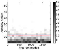
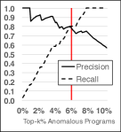
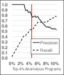
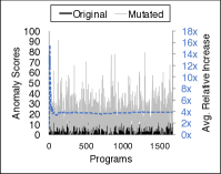
(a)	(b)(i)	(b)(ii)	(c)

Figure 5: (a) Histogram of anomaly score values, (b) Precision-recall for the possible bugs in Figure 6 for (i) Bayesian model (ii) non-Bayesian model, and (c) Anomaly scores of remaining 90% programs before and after mutation

#	Count	Avg		Anomaly
		Score
1	2	43.7	${\tt C}$	Single crypto object used to encrypt/decrypt multiple data
2	1	37.5	${\tt B}$	Connecting to the same socket more than once
3	1	24.7	${\tt B}$	Attempt to close unopened socket
4	16	22.1	${\tt A}$	Using ${\tt String}$ and ${\tt int}$ polymorphic methods together
5	6	21.8	${\tt C}$	Crypto object created without specifying mode
6	6	21.6	${\tt A}$	Using ${\tt setMessage}$ with ${\tt setView}$
7	1	19.8	${\tt A}$	Dialog displayed without message
8	1	19.3	${\tt B}$	Failed socket connection left unclosed
9	1	16.5	${\tt A}$	Unusual button text
10	1	15.7	${\tt A}$	Dialog displayed without buttons

Figure 6: Anomalies that are possible bugs, found in the top 10% of anomalous programs

To evaluate our method on anomaly detection, we first trained the topic-conditioned RNN on 60,000 behaviors sampled from the training programs. Training took 20 minutes to complete. We then computed anomaly scores for the 1800 programs in our testing corpus. The time to compute each score was around 2-3 seconds.

The histogram of scores, in Figure 5(a), shows a high concentration of small values, such as 5 or less, and a very low concentration of high values. We chose to further investigate programs appearing in the top 10% of anomaly scores (above the red line) for possible bugs. Specifically, since each program provides a localization to a location in the app (through its accepting states), we investigated the behaviors that were sampled from the program’s probabilistic behavior model, that would have determined its anomaly score.

Our definition of a “possible bug” is based on the following: is a behavior an instance of Android API usage that is questionable enough that we would expect it to be raised as an issue in a formal code review? Note that an issue raised in a code review may relate to a design choice and not necessarily cause the program to crash (an unusual button text, for example). Nonetheless, such an issue would be raised and likely fixed by engineers examining a code.

One problem with counting an anomaly as a possible bug is that multiple anomalies in an app can have the same “cause”—an incorrect statement or set of statements in the code—and we would like to avoid “double-counting” different anomalies with the same cause as different bugs. It is a hard software engineering problem to establish the cause of an anomaly/bug, which is out of scope of this paper. To avoid this problem, however, we conservatively consider only the top-most anomaly in each app in the top-10%, as clearly, anomalies in two different apps cannot have the same cause.

Through a manual inspection and triage by one of the authors, we found 10 different types of possible bugs in our testing corpus (Figure 6), ranging from the benign to the insidious. We have already seen instances of #6 and #10 (Figure 2) that could display corrupted or unclosable dialog boxes. #2 is serious as it could lead to an exception being thrown due to a failed connection. #5 would create a crypto object that defaults to the semantically insecure ECB-encryption mode. #8 is serious, and could cause future attempts to open a socket, even by other apps, to be blocked.

Figure 5(b)(i) shows the precision-recall plot for these possible bugs in the top-10% of anomaly scores. It can be seen that at around the top 8%, we reach full recall with 75% precision or 25% false positive rate. This is reasonable compared to industrial static analysis tools such as Coverity that advocates a 20% false positive rate for “stable” checkers Bessey et al. , [2010]. Our method does not rely on specified properties to check, and many of these bugs cannot be easily expressed as a formal property for traditional static analyzers to check.

After this threshold, the precision continues to drop, and we conjecture that it will not increase any further, because almost all the possible bugs have already been found. To substantiate this conjecture, we would have to manually inspect thousands of programs to qualitatively declare that all anomalies have been triaged. Due to the practical infeasibility of this task, we instead quantitatively injected anomalies into the remaining 90% of programs through mutations, and measured whether our model is able to detect those mutations. For each program, we mutated the API call before its accepting states into one chosen randomly from $\Sigma$.

Figure 5(c) shows the anomaly scores before (dark) and after (light) the mutation, and the cumulative mean of the relative increase in the score (dashed line, secondary axis). As a result of the mutation, the scores are greatly increased, sometimes by 20 times or more, and the mean of the increase is about 4x. That is, a mutation, on average, caused the anomaly score to increase by 4 times, indicating that our model detected the mutation.

Note that a random mutation, of course, has the possibility of reducing the anomaly score of a program if it had a possible bug and the mutation happened to fix it. However, since it is not very likely for a random mutation to fix a possible bug, these instances were few and far between.

5.4 Role of Learning in Anomaly Detection

To evaluate the role of learning, we compared with a traditional outlier detection method that does not require learning. k-nearest neighbor (k-NN) outlier detection Altman, [1992] uses a distance measure to compute the $k$ nearest neighbors of a given point within a dataset. The larger the average distance to the k-NN, the more likely it is that the point is an outlier, or anomaly. We already have a distance measure between distributions: the KL-divergence between the behavior model for the given program and a program in the corpus.

We implemented such a k-NN and compared our method with it by conservatively setting $k=1$. That is, the anomaly score of a given program is the smallest KL-divergence with any program in the corpus. However, even with this 1-NN anomaly score, a substantial top 25% of programs had a distance of infinity to the corpus, thus providing no useful information about their anomalies.

The reason is that these programs simply happened to generate a behavior that was not generated by any program in the corpus. This sets $P_{1}(\theta)$ to a non-zero value and $P_{2}(\theta)$ to zero in the KL-divergence formula (Equation 3) immediately making the sum infinity. This is unreasonable because we clearly do not want to call every behavior we have not observed in the training data an anomaly, but instead would like to assign probabilities even to behaviors that were never seen before. That is, we would like to generalize from the corpus. This is why probabilistic specification learning is needed.

5.5 Comparison with non-Bayesian methods

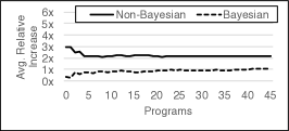
	(a)
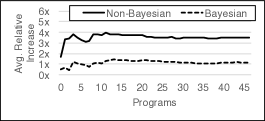
	(b)

Figure 7: Average relative increase in anomaly scores of ${\tt BluetoothSocket}$ programs when the training corpus only uses the APIs (a) ${\tt BluetoothSocket}$, ${\tt Cipher}$ (b) ${\tt AlertDialog.Builder}$, ${\tt BluetoothSocket}$, ${\tt Cipher}$

To see how the Bayesian framework helps in handling heterogeneity in the corpus, we compared our method with a non-Bayesian specification learning method. Existing state-of-the-art methods use n-grams Wang et al. , [2016a] or RNNs Raychev et al. , [2014] to learn a (non-Bayesian) single probabilistic specification of program behaviors. We implemented a non-Bayesian specification learner as an RNN (not topic conditioned) and trained it directly on the behaviors in our training corpus. We then performed the same anomaly and bug detection experiment in Section 5.3, querying the trained model with behaviors in the testing program for inference.

Figure 5(b)(ii) shows the precision-recall rate for the top-10% of anomaly scores. Compared to our Bayesian method, the non-Bayesian method performed poorly. Consider again a “stable” checker’s false-positive rate of 20%, or 80% precision. At this threshold (marked by the red line), our Bayesian method has about 80% recall compared to only 53% for the non-Bayesian method. This shows that given a reasonable precision threshold, our method is able to discover significantly more bugs compared to the non-Bayesian method. It is also worth noting that the non-Bayesian method was unable to discover any possible bug that was not found by our method.

Effect of Heterogeneity.

We finally performed a series of experiments by incrementally increasing the heterogeneity of the training programs. First, as a baseline, we considered only programs that use the ${\tt BluetoothSocket}$ API, and learned from them both Bayesian and non-Bayesian specifications of their behaviors. We then computed anomaly scores of the 45 testing programs that use this API.

In the next step, we added to the training corpus programs that also use the ${\tt Cipher}$ API, making the corpus more heterogeneous, and learned new specifications. We then computed anomaly scores again, but using the new learned specifications. Figure 7(a) shows the average relative increase in anomaly scores from using the old versus the new specifications. Ideally, one would expect the scores to not change, because the addition of programs that use the ${\tt Cipher}$ API—behaviors on which are unrelated to the ${\tt BluetoothSocket}$ API— should not have any effect on the scores. This is observed in the Bayesian specification (dashed line), that lingers close to 1.0 on average. However, the non-Bayesian specification (solid line) suffers from about a 2x increase.

This was further evident when programs that also use the API ${\tt AlertDialog.Builder}$ were considered for training, making the corpus even more heterogeneous (this is the same training corpus in Section 5.3). In Figure 7(b), the relative increase in scores using the Bayesian specification is, on average, close to 1.0, showing that it is robust to the increased heterogeneity. However, the non-Bayesian specification induces a further increase of about 3.5x in the scores.

We expect the gap to keep widening as more heterogeneous programs are added to the corpus, at some point making the scores from the non-Bayesian model meaningless. In contrast, the scores from our Bayesian model would remain almost the same showing that the model is able to “focus” on relevant parts of the learned specification, in principle tolerating arbitrary heterogeneity.

6 Related Work

Learning Qualitative Specifications.

The thesis that common patterns of execution can serve as a proxy for specifications has been around since the early 2000s. Most efforts in this area Ammons et al. , [2002, 2003]; Zhong et al. , [2009]; Li & Zhou, [2005]; Ernst et al. , [1999]; Nimmer & Ernst, [2002]; Weimer & Necula, [2005]; Alur et al. , [2005]; Goues & Weimer, [2009]; Shoham et al. , [2007]; Whaley et al. , [2002] focus on qualitative specifications, typically finite automata. As mentioned earlier, such qualitative specifications are problematic in the presence of noise in the training data.

Learning Probabilistic Specifications.

There is also a body of work  Ammons et al. , [2002]; Beckman & Nori, [2011]; Kremenek et al. , [2006]; Livshits et al. , [2009]; Octeau et al. , [2016]; Gvero et al. , [2013]; Raychev et al. , [2014] that uses machine learning techniques to learn probabilistic specifications from programs. Kremenek et al. Kremenek et al. , [2007, 2006] use factor graphs constructed using static analysis results to learn specifications on resource allocation and release. Anek Beckman & Nori, [2011] uses annotations in APIs to infer specifications. Merlin Livshits et al. , [2009] starts with a given initial specification and refines it through factor graph construction and inference. Octeau et al. Octeau et al. , [2016] use domain knowledge to train probabilistic models of Android inter-component communication. JSNice Raychev et al. , [2015] uses a probabilistic graphical model to learn lexical and syntactical properties of programs such as variable names and types for the purpose of de-obfuscating Javascript programs. Some recent efforts Nguyen et al. , [2013]; Nguyen & Nguyen, [2015]; Wang et al. , [2016a] have also used n-gram models to learn specifications on source code structure. DeepAPI Gu et al. , [2016] uses a neural encoder-decoder to learn correlations between natural language annotations and API sequences. Haggis Allamanis & Sutton, [2014] uses statistical techniques to learn the structure of small code snippets (or “idioms”) from a corpus. The work in this space that is perhaps the closest to ours are two papers by Raychev et al. Raychev et al. , [2014, 2016a]. These approaches learn probabilistic models of program behavior from large code corpora, using recurrent neural networks among other models.

The key difference between the above approaches and ours is that these methods learn a single probabilistic specification. In contrast, our approach learns a family of probabilistic specifications simultaneously, and then specializes this “big” model to particular analysis tasks using Bayes’ rule. As demonstrated in our experiments, this hierarchical architecture is key to tolerating heterogeneity.

In very recent work, Raychev et al. Raychev et al. , [2016b], also argue that having a single, universal probabilistic model for code can be inadequate, and propose a decision tree algorithm that is used to choose among a bag of statistical models for tasks such as next-statement prediction. While philosophically aligned with our work, their efforts are quite different in that while we argue for conditioning of models at the program level, they argue for conditioning of models at the statement level and focus their efforts on localized prediction tasks. One could imagine using a model similar to what they have proposed within our framework as a replacement for our RNN-based $P(\theta|\Psi)$.

Anomaly Detection.

There is prior work on using learned models of executions in anomaly detection Wasylkowski et al. , [2007]; Monperrus et al. , [2010]; Hangal & Lam, [2002]; Chilimbi & Ganapathy, [2006]; Baah et al. , [2006]; Gao et al. , [2007]; Fu et al. , [2009]; Wang et al. , [2016a]. Aside from differing in the nature of specifications used, methods in these categories tend to assign anomaly scores to individual behaviors (generated statically or dynamically). While our method is able to assign such scores, it is also able to produce aggregate anomaly scores for programs.

7 Conclusion

We have presented a Bayesian framework for learning probabilistic specifications from large, heterogeneous code corpora, and a method for finding likely software errors using this framework. We have used an implementation of this framework, based on a topic-model and a recurrent neural network, to detect API misuse in Android, and shown that it can find multiple subtle bugs.

A key appeal of our framework is that it does not impose an a priori limit on the size or heterogeneity of the corpus. In principle, our training corpus could contain all the world’s code, and it is our vision to scale our method to settings close to this ideal. Engineering instantiations of the framework that work at such scale is a challenge for future work.

Appendix A Constructing Program Models through Symbolic Execution

Here, we define the process that transforms a given program into a program model (Section 3) that our framework accepts as input. We consider a simple programming language that represents a program as a Control Flow Graph (CFG) $G$, where the vertices are the locations in the program $\{l_{1},\ldots,l_{n}\}$ and the edges are basic program operations from the following types: (i) assignments $x$:=$y$, (ii) assume statements assume($c$) that proceed with execution only if the Boolean condition $c$ is true, and (iii) method invocations $m(a_{1},\ldots,a_{k})$ that call the method $m$ with arguments $a_{1},\ldots,a_{k}$.

We construct the program model $F$ through a symbolic execution of the CFG $G$. Symbolic execution King, [1976]; Jaffar et al. , [2012]; Cadar et al. , [2008] executes a program with symbolic inputs, and keeps track of a symbolic state that is analogous to a program’s memory. A symbolic state is a tuple $\langle l,v\rangle$ where $l$ is a program location and $v$ is a symbolic store that is a mapping of variables to symbolic values. The symbolic states encountered during symbolic execution are exactly the states $\mathcal{Q}$ in the program model. The set of accepting states $Q_{A}$ typically consists of all states $\langle l,\cdot\rangle$ at a particular location $l$ in the program.

The evaluation of a symbolic expression $e$ in a symbolic store $v$, denoted as $\llbracket{e}\rrbracket_{v}$, is defined as usual: $\llbracket{x}\rrbracket_{v}=v(x)$, $\llbracket{k}\rrbracket_{v}=k$, $\llbracket{e_{1}+e_{2}}\rrbracket_{v}=\llbracket{e_{1}}\rrbracket_{v}+\llbracket{e_{2}}\rrbracket_{v}$, $\llbracket{e_{1}-e_{2}}\rrbracket_{v}=\llbracket{e_{1}}\rrbracket_{v}-\llbracket{e_{2}}\rrbracket_{v}$ and so on, where $x$ and $k$ are variables and constants, respectively. The evaluation of a Boolean condition $\llbracket{c}\rrbracket_{v}$ can also be defined in a similar manner. Note that $\llbracket{c}\rrbracket_{v}$ requires a theorem prover to evaluate, and the completeness of this theorem prover affects the exclusion of infeasible states from the program model.

Symbolic execution begins with an initial state $q_{0}=\langle l_{0},\emptyset\rangle$ where $l_{0}$ is the (special) initial location of the program with an empty store. Then, recursively, given a state $q=\langle l,v\rangle$, symbolic execution proceeds as follows:

• If $G$ has an edge from $l$ to $l^{\prime}$ where the operation is $x$:=$y$, then $q^{\prime}=\langle l^{\prime},v[x\mapsto\llbracket{y}\rrbracket_{v}]\rangle$ is added to $\mathcal{Q}$ and $q~{}\xrightarrow{\epsilon,1}~{}q^{\prime}$ is added to $\delta$, where $\epsilon$ is the empty symbol in $\Sigma$.

• If $G$ has edges from $l$ to $l_{1}^{\prime},\ldots,l_{m}^{\prime}$ with operations assume($c_{1}$), $\ldots$, assume($c_{m}$) respectively, then each condition is first evaluated for satisfiability: let $C$ be the set $\{l_{j}^{\prime}~{}|~{}\llbracket{c_{j}}\rrbracket_{v}=true\}$. Then, for each $l_{j}^{\prime}$ in $C$, a state $q_{j}^{\prime}=\langle l_{j}^{\prime},v\rangle$ is added to $\mathcal{Q}$ and $l~{}\xrightarrow{\epsilon,1/|C|}~{}l_{j}^{\prime}$ is added to $\delta$. By default, we give a uniform probability of $1/|C|$ to all feasible branches, but this can be enhanced if the distribution of inputs to the program is known, or through external techniques such as model counting.

• If $G$ has an edge from $l$ to $l^{\prime}$ with the operation $m(a_{1},\ldots,a_{k})$, then a state $q^{\prime}=\langle l^{\prime},v\rangle$ is added to $\mathcal{Q}$, and a transition $q~{}\xrightarrow{m,1}~{}q^{\prime}$ is added to $\delta$ if $m$ is in the alphabet $\Sigma$, otherwise, $q~{}\xrightarrow{\epsilon,1}~{}q^{\prime}$ is added to $\delta$.

Appendix B Counteracting Bias in Anomaly Scores

As mentioned before, the estimator used to compute anomaly scores is biased because the logarithm and expectation operators do not commute. However, we can develop an algorithm to counter-act the bias in estimating the bias of a sampling-based estimator for a logarithm using a Taylor series expansion. Assume that we have an estimator of the form $X=\sum_{s\in S}f(s)$ for some sample set $S$ and function $f(s)$; there are two such estimators in the computation of the anomaly score algorithm of Section 4.4. Also let $\hat{p}$ denote $E[X]$. Expanding the Taylor series for $\log(X)$ around the point $\hat{p}$ we have $\log(X)=$

$$\log(\hat{p})+\frac{(X-\hat{p})}{\hat{p}}-\frac{(X-\hat{p})^{2}}{2\hat{p}^{2}}+\frac{(X-\hat{p})^{3}}{3\hat{p}^{3}}-\frac{(X-\hat{p})^{4}}{4\hat{p}^{4}}+...$$

So, $E[\log(X)]=$

$$\log(\hat{p})+\frac{E[(X-\hat{p})]}{\hat{p}}-\frac{E[(X-\hat{p})^{2}]}{2\hat{p}^{2}}+\frac{E[(X-\hat{p})^{3}]}{3\hat{p}^{3}}-...$$

Then the bias is $E[\log(X)]-\log(E[X])$, or

$$\frac{E[(X-\hat{p})]}{\hat{p}}-\frac{E[(X-\hat{p})^{2}]}{2\hat{p}^{2}}+\frac{E[(X-\hat{p})^{3}]}{3\hat{p}^{3}}-...$$

The numerator in the $i$th term in this series corresponds to the $i$th central moment of $X$. Since $X$ is computed as an average of a number of independent, identically distributed samples, according to the Central Limit Theorem, $X$ is asymptotically normally distributed. Given this, and using the central moments of the normal distribution, we can write the bias as:

$$-\frac{\sigma^{2}(X)}{2\hat{p}^{2}}-\frac{3\sigma^{4}(X)}{4\hat{p}^{4}}-\frac{15\sigma^{6}(X)}{6\hat{p}^{6}}-\frac{105\sigma^{8}(X)}{8\hat{p}^{8}}-...$$

In practice, an estimate that takes into account the first three or four terms should be adequate. When estimating those terms, $\hat{p}$ can be estimated using the observed value of $X$; that is, $\hat{p}\approx\sum_{s\in S}f(s)$. $\sigma^{2}(X)$ is the variance of $X$ and can be estimated in many ways; we advocate using a bootstrap resampling procedure Efron & Tibshirani, [1994]. That is, we uniformly resample (with replacement) a set $S^{\prime}$ of $|S|$ items from $S$, and use this to produce a simulated value $\sum_{s\in S^{\prime}}f(s)$ for $\hat{p}$. We perform this resampling procedure many times, and use the observed variance as an estimate for $\sigma^{2}(X)$. In this way, it is possible to obtain an estimate for $bias(\theta,\Pi^{\prime}_{F},\psi_{F})$. Plugging this into the equation at the end of Section 4.4 then gives us our final estimator.

One last issue to consider is how to to compute the variance of this estimator so that we can know the error of our estimate and stop sampling at the appropriate time. We also advocate a bootstrap resampling procedure for this task. We simply re-sample $m$ $(\theta,\Pi^{\prime}_{F},\psi_{F})$ triples from the set of sampled $(\theta,\Pi^{\prime}_{F},\psi_{F})$ triples. We then compute Section 4.4’s estimator for each such triple. Taking the average value over all of the triples produces a simulated estimate for the anomaly score. Repeating this process many times and computing the empirically observed variance produces an estimate for the variance of the anomaly score.

Appendix C Gibbs Sampling to Approximate $P(\Psi|X;\textbf{M})$

LDA models a document as a distribution over topics, and a topic as a distribution over words in the vocabulary. An LDA model is thus fully characterized by the following variables: (i) $\alpha$ and $\eta$, hyper-parameters of a Dirichlet prior that chooses the topic distribution of each document and the word distribution of each topic, respectively (ii) $\Psi_{F_{i}}$, the topic distribution of document $X_{F_{i}}$, (iii) $\beta_{k}$, the word distribution of topic $t_{k}$, (iv) $z_{i,j}$, the topic that generated word $j$ in document $i$, and (v) $w_{i,j}$, the $j$th word in document $i$. With these parameters, the generative process of documents, according to LDA, is as follows:

• Decide on a topic distribution for document $X_{F_{i}}$: $\Psi_{F_{i}}\sim\mbox{Dir}_{K}(\alpha)$, where $\alpha$ is a $K$-length vector of reals. This sampling would produce a distribution over $K$ topics.

• Decide on a word distribution for topic $t_{k}$: $\beta_{k}\sim\mbox{Dir}_{|\Sigma|}(\eta)$.

• For each word position $i,j$, $1\leq i\leq M$ and $1\leq j\leq N_{i}$,

  • Decide on a topic for the word to be generated at $i,j$: $z_{i,j}\sim\mbox{Categorical}_{K}(\Psi_{F_{i}})$.

  • Generate the word: $w_{i,j}\sim\mbox{Categorical}_{|\Sigma|}(\beta_{z_{i,j}})$.

The total probability of all variables in the model is then

$$\prod_{k=1}^{K}P(\beta_{k}|\eta)\prod_{i=1}^{M}P(\Psi_{F_{i}}|\alpha)\prod_{j=1}^{N}P(z_{i,j}|\Psi_{F_{i}})P(w_{i,j}|\beta_{z_{i,j}})$$

We refer the reader to Blei et al. , [2003] for details on training an LDA model. The result of training is a learned value for all latent variables in the model, particularly all the $\beta_{k}$. During inference, we are given a particular $X_{F}$ and would like to compute the posterior distribution $P(\Psi|X_{F};\textbf{M})$.

In LDA terms, $\Psi$ would be a topic distribution for $X_{F}$ (we drop the $i$ subscript since we are now only working with one document). In order to estimate this distribution, we employ a standard Markov Chain Monte Carlo (MCMC) method called Gibbs sampling. First, we sample $\Psi$ from a Dirichlet prior parameterized by some randomly chosen $d$: $\Psi\sim\mbox{Dir}_{K}(d)$. Then, each step of Gibbs sampling re-computes $\Psi$ using Bayes’ rule:

• For every word $w_{j}$ in $X_{F}$, decide on a topic $t_{k}$ that could have generated $w_{j}$ by sampling from the distribution

  $$P(t_{k}|w_{j})=\frac{P(w_{j}|t_{k})P(t_{k})}{P(w_{j})}$$

  where $P(w_{j}|t_{k})$ is the probability of the word $w_{j}$ according the learned model $\beta_{k}$, $P(t_{k})$ is obtained from the current value of $\Psi$ and $P(w_{j})=\sum_{k=1}^{K}P(w_{j}|t_{k})P(t_{k})$ is a normalization term.

• Compute the vector $n=(n_{1},\ldots,n_{K})$ where $n_{k}$ is the number of words in $X_{F}$ that were generated by topic $t_{k}$.

• Re-sample $\Psi$ from the distribution $\Psi\sim\mbox{Dir}_{K}(d+n)$.

Gibbs sampling guarantees that by repeating these steps for some number of iterations (that depends on the value of $d$), the samples of $\Psi$ would eventually converge to coming from the posterior distribution $P(\Psi|X_{F};\textbf{M})$, thus approximating this distribution through sampling.

References

- and, [n.d.] AndroidDrawer. http://www.androiddrawer.com. [Online; accessed 06-Jul-2016].
- fdr, [n.d.] F-Droid. https://f-droid.org. [Online; accessed 06-Jul-2016].
- Abadi et al. , [2015] Abadi, Martín, Agarwal, Ashish, Barham, Paul, Brevdo, Eugene, Chen, Zhifeng, Citro, Craig, Corrado, Greg, Davis, Andy, Dean, Jeffrey, Devin, Matthieu, Ghemawat, Sanjay, Goodfellow, Ian, Harp, Andrew, Irving, Geoffrey, Isard, Michael, Jia, Yangqing, Jozefowicz, Rafal, Kaiser, Lukasz, Kudlur, Manjunath, Levenberg, Josh, Mané, Dan, Monga, Rajat, Moore, Sherry, Murray, Derek, Olah, Chris, Schuster, Mike, Shlens, Jonathon, Steiner, Benoit, Sutskever, Ilya, Talwar, Kunal, Tucker, Paul, Vanhoucke, Vincent, Vasudevan, Vijay, Viégas, Fernanda, Vinyals, Oriol, Warden, Pete, Wattenberg, Martin, Wicke, Martin, Yu, Yuan, & Zheng, Xiaoqiang. 2015. TensorFlow: Large-Scale Machine Learning on Heterogeneous Distributed Systems.
- Allamanis & Sutton, [2014] Allamanis, Miltiadis, & Sutton, Charles. 2014. Mining Idioms from Source Code. Pages 472–483 of: Proceedings of the 22Nd ACM SIGSOFT International Symposium on Foundations of Software Engineering. FSE 2014. New York, NY, USA: ACM.
- Altman, [1992] Altman, Naomi S. 1992. An introduction to kernel and nearest-neighbor nonparametric regression. The American Statistician, 46(3), 175–185.
- Alur et al. , [2005] Alur, Rajeev, Černý, Pavol, Madhusudan, P., & Nam, Wonhong. 2005. Synthesis of Interface Specifications for Java Classes. Pages 98–109 of: POPL.
- Ammons et al. , [2002] Ammons, Glenn, Bodík, Rastislav, & Larus, James R. 2002. Mining specifications. Pages 4–16 of: POPL.
- Ammons et al. , [2003] Ammons, Glenn, Mandelin, David, & Larus, James R. 2003. Debugging temporal specifications with concept analysis. Pages 182–195 of: In ACM SIGPLAN Conf on Prog Lang Design and Implem. ACM Press.
- Anand et al. , [2007] Anand, Saswat, Păsăreanu, Corina S, & Visser, Willem. 2007. JPF–SE: A symbolic execution extension to java pathfinder. Pages 134–138 of: International Conference on Tools and Algorithms for the Construction and Analysis of Systems. Springer.
- Baah et al. , [2006] Baah, George K, Gray, Alexander, & Harrold, Mary Jean. 2006. On-line anomaly detection of deployed software: a statistical machine learning approach. Pages 70–77 of: Proceedings of the 3rd international workshop on Software quality assurance. ACM.
- Ball et al. , [2011] Ball, Thomas, Levin, Vladimir, & Rajamani, Sriram K. 2011. A Decade of Software Model Checking with SLAM. Commun. ACM, 54(7), 68–76.
- Beckman & Nori, [2011] Beckman, Nels E., & Nori, Aditya V. 2011. Probabilistic, Modular and Scalable Inference of Typestate Specifications. SIGPLAN Not., 46(6), 211–221.
- Bengio et al. , [2003] Bengio, Yoshua, Ducharme, Réjean, Vincent, Pascal, & Jauvin, Christian. 2003. A neural probabilistic language model. journal of machine learning research, 3(Feb), 1137–1155.
- Bessey et al. , [2010] Bessey, Al, Block, Ken, Chelf, Ben, Chou, Andy, Fulton, Bryan, Hallem, Seth, Henri-Gros, Charles, Kamsky, Asya, McPeak, Scott, & Engler, Dawson. 2010. A Few Billion Lines of Code Later: Using Static Analysis to Find Bugs in the Real World. Communications of the ACM, 53(2), 66–75.
- Blei et al. , [2003] Blei, David M., Ng, Andrew Y., & Jordan, Michael I. 2003. Latent Dirichlet Allocation. Journal of Machine Learning Research, 3, 993–1022.
- Cadar et al. , [2008] Cadar, Cristian, Dunbar, Daniel, & Engler, Dawson. 2008. KLEE: Unassisted and Automatic Generation of High-coverage Tests for Complex Systems Programs. Pages 209–224 of: Proceedings of the 8th USENIX Conference on Operating Systems Design and Implementation. OSDI’08. Berkeley, CA, USA: USENIX Association.
- Chilimbi & Ganapathy, [2006] Chilimbi, Trishul M, & Ganapathy, Vinod. 2006. Heapmd: Identifying heap-based bugs using anomaly detection. Pages 219–228 of: ASPLOS, vol. 34. ACM.
- Efron & Tibshirani, [1994] Efron, Bradley, & Tibshirani, Robert J. 1994. An introduction to the bootstrap. CRC press.
- Engler et al. , [2001] Engler, Dawson R., Chen, David Yu, & Chou, Andy. 2001. Bugs as Inconsistent Behavior: A General Approach to Inferring Errors in Systems Code. Pages 57–72 of: SOSP.
- Ernst et al. , [1999] Ernst, Michael D., Cockrell, Jake, Griswold, William G., & Notkin, David. 1999. Dynamically Discovering Likely Program Invariants to Support Program Evolution. Pages 213–224 of: ICSE.
- Fu et al. , [2009] Fu, Qiang, Lou, Jian-Guang, Wang, Yi, & Li, Jiang. 2009. Execution Anomaly Detection in Distributed Systems through Unstructured Log Analysis. Pages 149–158 of: ICDM, vol. 9.
- Gao et al. , [2007] Gao, Qi, Qin, Feng, & Panda, Dhabaleswar K. 2007. DMTracker: finding bugs in large-scale parallel programs by detecting anomaly in data movements. Page 15 of: Proceedings of the 2007 ACM/IEEE conference on Supercomputing. ACM.
- Geman & Geman, [1984] Geman, Stuart, & Geman, Donald. 1984. Stochastic Relaxation, Gibbs Distributions, and the Bayesian Restoration of Images. IEEE Trans. Pattern Anal. Mach. Intell., 6(6), 721–741.
- Goues & Weimer, [2009] Goues, Claire, & Weimer, Westley. 2009. Specification Mining with Few False Positives. Pages 292–306 of: TACAS.
- Gu et al. , [2016] Gu, Xiaodong, Zhang, Hongyu, Zhang, Dongmei, & Kim, Sunghun. 2016. Deep API Learning. CoRR, abs/1605.08535.
- Gvero et al. , [2013] Gvero, Tihomir, Kuncak, Viktor, Kuraj, Ivan, & Piskac, Ruzica. 2013. Complete Completion Using Types and Weights. SIGPLAN Not., 48(6), 27–38.
- Hangal & Lam, [2002] Hangal, Sudheendra, & Lam, Monica S. 2002. Tracking down software bugs using automatic anomaly detection. Pages 291–301 of: Proceedings of the 24th international conference on Software engineering. ACM.
- Jaffar et al. , [2012] Jaffar, Joxan, Murali, Vijayaraghavan, Navas, Jorge A., & Santosa, Andrew E. 2012. TRACER: A Symbolic Execution Tool for Verification. Pages 758–766 of: Proceedings of the 24th International Conference on Computer Aided Verification. CAV’12. Berlin, Heidelberg: Springer-Verlag.
- Jones et al. , [2001–] Jones, Eric, Oliphant, Travis, Peterson, Pearu, et al. . 2001–. SciPy: Open source scientific tools for Python. [Online; accessed 2016-11-09].
- King, [1976] King, James C. 1976. Symbolic Execution and Program Testing. Commun. ACM, 19(7), 385–394.
- Kremenek et al. , [2006] Kremenek, Ted, Twohey, Paul, Back, Godmar, Ng, Andrew, & Engler, Dawson. 2006. From Uncertainty to Belief: Inferring the Specification Within. Pages 161–176 of: Proceedings of the 7th Symposium on Operating Systems Design and Implementation. OSDI ’06. Berkeley, CA, USA: USENIX Association.
- Kremenek et al. , [2007] Kremenek, Ted, Ng, Andrew Y., & Engler, Dawson. 2007. A Factor Graph Model for Software Bug Finding. Pages 2510–2516 of: Proceedings of the 20th International Joint Conference on Artifical Intelligence. IJCAI’07. San Francisco, CA, USA: Morgan Kaufmann Publishers Inc.
- Kullback & Leibler, [1951] Kullback, S., & Leibler, R. A. 1951. On Information and Sufficiency. Ann. Math. Statist., 22(1), 79–86.
- Li & Zhou, [2005] Li, Zhenmin, & Zhou, Yuanyuan. 2005. PR-Miner: Automatically Extracting Implicit Programming Rules and Detecting Violations in Large Software Code. Pages 306–315 of: Proceedings of the 10th European Software Engineering Conference Held Jointly with 13th ACM SIGSOFT International Symposium on Foundations of Software Engineering. ESEC/FSE-13. New York, NY, USA: ACM.
- Livshits et al. , [2009] Livshits, Benjamin, Nori, Aditya V., Rajamani, Sriram K., & Banerjee, Anindya. 2009. Merlin: Specification Inference for Explicit Information Flow Problems. Pages 75–86 of: Proceedings of the 30th ACM SIGPLAN Conference on Programming Language Design and Implementation. PLDI ’09.
- Mikolov & Zweig, [2012] Mikolov, Tomas, & Zweig, Geoffrey. 2012. Context dependent recurrent neural network language model. Pages 234–239 of: SLT.
- Monperrus et al. , [2010] Monperrus, Martin, Bruch, Marcel, & Mezini, Mira. 2010. Detecting Missing Method Calls in Object-oriented Software. Pages 2–25 of: Proceedings of the 24th European Conference on Object-oriented Programming. ECOOP’10. Berlin, Heidelberg: Springer-Verlag.
- Murawski & Ouaknine, [2005] Murawski, Andrzej S., & Ouaknine, Joël. 2005. CONCUR 2005 - Concurrency Theory. London, UK, UK: Springer-Verlag.
- Nguyen & Nguyen, [2015] Nguyen, Anh Tuan, & Nguyen, Tien N. 2015. Graph-based Statistical Language Model for Code. Pages 858–868 of: Proceedings of the 37th International Conference on Software Engineering - Volume 1. ICSE ’15. Piscataway, NJ, USA: IEEE Press.
- Nguyen et al. , [2013] Nguyen, Tung Thanh, Nguyen, Anh Tuan, Nguyen, Hoan Anh, & Nguyen, Tien N. 2013. A Statistical Semantic Language Model for Source Code. Pages 532–542 of: Proceedings of the 2013 9th Joint Meeting on Foundations of Software Engineering. ESEC/FSE 2013. New York, NY, USA: ACM.
- Nimmer & Ernst, [2002] Nimmer, Jeremy W., & Ernst, Michael D. 2002 (July 22–24,). Automatic generation of program specifications. Pages 232–242 of: ISSTA 2002, Proceedings of the 2002 International Symposium on Software Testing and Analysis.
- Octeau et al. , [2016] Octeau, Damien, Jha, Somesh, Dering, Matthew, McDaniel, Patrick, Bartel, Alexandre, Li, Li, Klein, Jacques, & Le Traon, Yves. 2016. Combining Static Analysis with Probabilistic Models to Enable Market-scale Android Inter-component Analysis. Pages 469–484 of: Proceedings of the 43rd Annual ACM SIGPLAN-SIGACT Symposium on Principles of Programming Languages. POPL 2016.
- Raychev et al. , [2014] Raychev, Veselin, Vechev, Martin, & Yahav, Eran. 2014. Code Completion with Statistical Language Models. Pages 419–428 of: Proceedings of the 35th ACM SIGPLAN Conference on Programming Language Design and Implementation. PLDI ’14.
- Raychev et al. , [2015] Raychev, Veselin, Vechev, Martin, & Krause, Andreas. 2015. Predicting program properties from Big Code. Pages 111–124 of: POPL, vol. 50.
- Raychev et al. , [2016a] Raychev, Veselin, Bielik, Pavol, Vechev, Martin T., & Krause, Andreas. 2016a. Learning programs from noisy data. Pages 761–774 of: Proceedings of the 43rd Annual ACM SIGPLAN-SIGACT Symposium on Principles of Programming Languages, POPL 2016, St. Petersburg, FL, USA, January 20 - 22, 2016.
- Raychev et al. , [2016b] Raychev, Veselin, Bielik, Pavol, & Vechev, Martin T. 2016b. Probabilistic model for code with decision trees. Pages 731–747 of: Proceedings of the 2016 ACM SIGPLAN International Conference on Object-Oriented Programming, Systems, Languages, and Applications, OOPSLA 2016, part of SPLASH 2016, Amsterdam, The Netherlands, October 30 - November 4, 2016.
- Shoham et al. , [2007] Shoham, Sharon, Yahav, Eran, Fink, Stephen, & Pistoia, Marco. 2007. Static Specification Mining Using Automata-based Abstractions. Pages 174–184 of: Proceedings of the 2007 International Symposium on Software Testing and Analysis. ISSTA ’07. New York, NY, USA: ACM.
- Sokolova & de Vink, [2004] Sokolova, Ana, & de Vink, Erik P. 2004. Probabilistic Automata: System Types, Parallel Composition and Comparison. Berlin, Heidelberg: Springer Berlin Heidelberg. Pages 1–43.
- Vallée-Rai et al. , [1999] Vallée-Rai, Raja, Co, Phong, Gagnon, Etienne, Hendren, Laurie, Lam, Patrick, & Sundaresan, Vijay. 1999. Soot - a Java Bytecode Optimization Framework. Pages 13– of: Proceedings of the 1999 Conference of the Centre for Advanced Studies on Collaborative Research. CASCON ’99. IBM Press.
- Von Neumann, [1951] Von Neumann, John. 1951. 13. Various Techniques Used in Connection With Random Digits.
- Wang et al. , [2016a] Wang, Song, Chollak, Devin, Movshovitz-Attias, Dana, & Tan, Lin. 2016a. Bugram: Bug Detection with N-gram Language Models. Pages 708–719 of: Proceedings of the 31st IEEE/ACM International Conference on Automated Software Engineering. ASE 2016. New York, NY, USA: ACM.
- Wang et al. , [2016b] Wang, Song, Chollak, Devin, Movshovitz-Attias, Dana, & Tan, Lin. 2016b. Bugram: bug detection with n-gram language models. Pages 708–719 of: Proceedings of the 31st IEEE/ACM International Conference on Automated Software Engineering, ASE 2016, Singapore, September 3-7, 2016.
- Wasylkowski et al. , [2007] Wasylkowski, Andrzej, Zeller, Andreas, & Lindig, Christian. 2007. Detecting Object Usage Anomalies. Pages 35–44 of: Proceedings of the the 6th Joint Meeting of the European Software Engineering Conference and the ACM SIGSOFT Symposium on The Foundations of Software Engineering. ESEC-FSE ’07. New York, NY, USA: ACM.
- Weimer & Necula, [2005] Weimer, Westley, & Necula, George C. 2005. Mining Temporal Specifications for Error Detection. Pages 461–476 of: Proceedings of the 11th International Conference on Tools and Algorithms for the Construction and Analysis of Systems. TACAS’05.
- Whaley et al. , [2002] Whaley, John, Martin, Michael C., & Lam, Monica S. 2002. Automatic Extraction of Object-oriented Component Interfaces. Pages 218–228 of: Proceedings of the 2002 ACM SIGSOFT International Symposium on Software Testing and Analysis. ISSTA ’02. New York, NY, USA: ACM.
- Zhong et al. , [2009] Zhong, Hao, Xie, Tao, Zhang, Lu, Pei, Jian, & Mei, Hong. 2009. MAPO: Mining and Recommending API Usage Patterns. Pages 318–343 of: Proceedings of the 23rd European Conference on ECOOP 2009 — Object-Oriented Programming. Genoa.