Sampling and Frequency Warping

Abstract.

Optimal sampling of non band-limited functions is an issue of great importance that has attracted considerable attention. We propose to tackle this problem through the use of a frequency warping: First, by a non-linear shrinking of frequencies, the function is transformed into a band-limited one. One may then perform a decomposition in Fourier series. This process gives rise to new orthonormal bases of the Sobolev spaces ${\mathcal{H}}^{\alpha}$. When $\alpha$ is an integer, these orthonormal bases can be expressed in terms of Laguerre functions. We study the reconstruction and speed of convergence properties of the warping-based sampling. Besides theoretical considerations, numerical experiments are performed.

1. Introduction

Sampling theory is a rich research topic that lies at the boundary between harmonic analysis and signal processing. The basic result is the Whittaker-Kotelnikov-Shannon theorem (WKS) [4, 8]: From a signal processing point of view, it tells that it is possible to reconstruct exactly a band-limited signal, i.e., a signal whose Fourier transform is compactly supported in $(-1/2,1/2)$, from regularly spaced samples provided the sampling frequency is not smaller than 1. From a theoretical point of view, it asserts the identity between the space of functions in $L^{2}(\mathbb{R})$ whose Fourier transform vanishes outside $(-1/2,1/2)$ and the space $\{\sum_{k\in\mathbb{Z}}c_{k}\operatorname{sinc}(t-k),(c_{k})_{k}\in l^{2}\}$, where $\operatorname{sinc}t=\sin\pi t/\pi t$ .

A huge literature has been devoted to generalizing the WKS theorem in various directions. Classical extensions include the case of non-regular sampling, multichannel sampling, or the sampling and reconstruction of functions in more general spaces. See [1, 3, 6, 7] for excellent reviews.

We propose the following treatment. We are given an increasing function $\varphi$ from the interval $(-\frac{\pi}{2},\frac{\pi}{2})$ onto ${\mathbb{R}}$. Then one can expand $\widehat{X}\circ\varphi$ in Fourier series. The coefficients $a_{n}$ of this expansion bear the whole information contained in $X$. Indeed, the original signal, when it lies in a Sobolev space, can be decomposed as the sum of a series $\displaystyle\sum_{n\in{\mathbb{Z}}}a_{n}\gamma_{n}$, where the $\gamma_{n}$ form an orthogonal basis of the Sobolev space under consideration.

First, in Section 2, we develop a general setting and define the warping operators. Afterwards, In Section 3, we particularise the situation and are able to derive formulas for the aforementioned $\gamma_{n}$ which involve known special functions.

In Section 4, we examine the speed of approximation and compare the warping method to the usual sampling. In the last section, we give an account of computations an simulations. In particular we test and compare on several signals the efficiency of its representations either by sampling or by warping.

2. The general warping operators

2.1. Preliminaries and notation

For the Fourier transform of a function $X\in L^{1}({\mathbb{R}})$, we use the following convention:

$${\widehat{X}}(\omega)=\int_{\mathbb{R}}X(t){\mathrm{e}}^{-\mathrm{i}t\omega}\mathrm{d}t.$$

If $X$ and $Y$ are two functions in $L^{2}({\mathbb{R}})$, their scalar product $\int_{\mathbb{R}}X(t)\,\overline{Y(t)}\,\mathrm{d}t$ is denoted by $\langle X,Y\rangle$. We use the same notation if $X\in{\mathcal{S}}^{\prime}({\mathbb{R}})$ and $Y\in{\mathcal{S}}({\mathcal{R}})$.

The Heaviside function will be denoted by $H$. The symbol $\delta$ stands either for the Dirac measure or the Kronecker sumbol, depending on the context.

If $u\in{\mathbb{R}}$ and $j\in{\mathbb{N}}$, we define the generalized binomial coefficient to be

$$\binom{u}{j}=\frac{u(u-1)...(u-j+1)}{j!}$$

if $j>0$, and 1 if $j=0$. With this convention, for all $u\in{\mathbb{R}}$ and $|x|<1$, one has $(1+x)^{u}=\sum_{j\geq 0}\binom{u}{j}\,x^{j}$.

We also have the following formula

(2.1) $$\binom{-u}{j}=(-1)^{j}\,\binom{u+j-1}{j}.$$

We will use some special functions, namely the Whittaker function $W$ ([5], p. 88) and the generalized Laguerre polynomials ([9], p. 100)

$$L_{n}^{(\alpha)}(x)=\frac{1}{n!}\,x^{-\alpha}{\mathrm{e}}^{x}\left(\frac{\mathrm{d}}{\mathrm{d}x}\right)^{n}\Bigl{(}x^{n+\alpha}{\mathrm{e}}^{-x}\Bigr{)}=\sum_{j=0}^{n}\binom{n+\alpha}{n-j}\,\frac{(-x)^{j}}{j!},$$

where $n\in{\mathbb{N}}$ and $\alpha\in{\mathbb{R}}$.

When the parameter $\alpha$ is larger than $-1$, one has the following orthogonality relation

$$\int_{o}^{+\infty}L_{n}^{(\alpha)}(x)\,L_{m}^{(\alpha)}(x)\,x^{\alpha}{\mathrm{e}}^{-x}\,dx=\Gamma(\alpha+1)\,\binom{n+\alpha}{n}\,\delta_{n,m}.$$

2.2. The warping operators

We are given $\psi$, an increasing $C^{1}$ function from ${\mathbb{R}}$ onto an open interval $I$ of ${\mathbb{R}}$, and $\chi$ a positive function defined on $I$.

The length of the interval $I$, when it is bounded, will be denoted by $|I|$ and the mapping reciprocal to $\psi$ by $\varphi$. We set $\varpi=(\chi\circ\psi)^{2}.\psi^{\prime}$.

Let ${\mathcal{H}}_{\varpi}$ stand for the set of distributions $X$ on ${\mathbb{R}}$ the Fourier transform of which is a function $\widehat{X}$ such that $\displaystyle\int_{\mathbb{R}}|\widehat{X}(\omega)|^{2}\varpi(\omega)\,\mathrm{d}\omega$ is finite. This definition makes sense when $1/\varpi$ has a polynomial growth.

We always assume that both $\boldsymbol{\varpi}$ and $\mathbf{1}\boldsymbol{/\varpi}$ have polynomial growth.

If $X\in{\mathcal{H}}_{\varpi}$, one has

$$\int_{I}|\widehat{X}\bigl{(}\varphi(u)\bigr{)}\,\chi(u)|^{2}\mathrm{d}u = \int_{\mathbb{R}}|\widehat{X}(\omega)\,\chi\bigl{(}\psi(\omega)\bigr{)}|^{2}\psi^{\prime}(\omega)\,\mathrm{d}\omega$$

$$= \int_{\mathbb{R}}|\widehat{X}(\omega)|^{2}\varpi(\omega)\,\mathrm{d}\omega<+\infty.$$

This legitimates the following definition.

Definition 1 (Warping operator).

Given $\psi$ and $\chi$, we define the warping operator ${\mathcal{T}}^{\psi,\chi}$ as follows:

$${\mathcal{T}}^{\psi,\chi}:\left(\begin{array}[]{ccc}{\mathcal{H}}_{\varpi}&\longrightarrow&L^{2}(I,\mathrm{d}u)\\ X&\longmapsto&(\widehat{X}\circ\varphi).\chi\end{array}\right)$$

In view of Formula 2.2, the operator ${\mathcal{T}}^{\psi,\chi}$ is an isometry from ${\mathcal{H}}_{\varpi}$ onto $L^{2}(I)$. Therefore, if $\{e_{n}\}_{n\in{\mathbb{Z}}}$ is an orthonormal basis of $L^{2}(I)$, one gets an orthonormal basis $\{\gamma_{n}\}_{n\in{\mathbb{Z}}}$ of ${\mathcal{H}}_{\varpi}$ in the following way:

(2.3) $$\widehat{\gamma}_{n}(\omega)=e_{n}\circ\psi(\omega)/\chi\bigl{(}\psi(\omega)\bigr{)}=\sqrt{\frac{\psi^{\prime}(\omega)}{\varpi(\omega)}}\,e_{n}\bigl{(}\psi(\omega)\bigr{)}.$$

As a consequence, any $X\in{\mathcal{H}}_{\varpi}$, can be expanded in ${\mathcal{H}}_{\varpi}$ as the sum

$$X=\sum_{k\in{\mathbb{Z}}}\langle X,\gamma_{k}\rangle_{{\mathcal{H}}_{\varpi}}\,\gamma_{k}.$$

In this decomposition, the coefficients $\langle f,\gamma_{k}\rangle_{{\mathcal{H}}_{\varpi}}$ are expressed in terms of the inner product of ${\mathcal{H}}_{\varpi}$. However, in practice, it is useful to have an expression of these coefficients as a distributional duality product (so that we merely need to know $X$ and not ${\widehat{X}}$).

As ${\mathcal{H}}_{1/\varpi}$ is isometrically isomorphic to the dual of ${\mathcal{H}}_{\varpi}$, one has

(2.4) $$X=2\pi\sum_{n\in{\mathbb{Z}}}\langle X,\widetilde{\gamma}_{n}\rangle\,\gamma_{n},$$

where $\displaystyle\widehat{\widetilde{\gamma}}_{n}=\varpi\,\widehat{\gamma}_{n}=\sqrt{\varpi\,\psi^{\prime}}\,e_{n}\circ\psi$, and the scalar product is the usual pairing of functions and distributions. One can notice that the $\widetilde{\gamma}_{n}$ arise from the preceding construction with the same function $\psi$ but with $\varphi^{\prime}/\chi$ instead of $\chi$.

3. The case $\psi=\arctan$

In this case we choose for $\chi$ the function $(1+\tan^{2})^{\frac{1+\alpha}{2}}$, where $\alpha$ is a real parameter. The corresponding warping operator will be denoted by ${\mathcal{T}}_{\alpha}$. Then $I=(-\pi/2,\pi/2)$ and $\varpi(\omega)=\chi(\arctan\omega)^{2}/(1+\omega^{2})=(1+\omega^{2})^{\alpha}$. It results that the space ${\mathcal{H}}_{\varpi}$ is the ordinary Sobolev space ${\mathcal{H}}^{\alpha}({\mathbb{R}})$.

3.1. A family of orthonormal bases

Choose a real parameter $\beta$. Then the system of functions $e_{n}(u)={\mathrm{e}}^{-2\mathrm{i}n\,u}/\sqrt{\pi}$  (for $n\in\beta+{\mathbb{Z}}$) is an orthonormal basis of $L^{2}(I)$. The corresponding $\gamma_{n}$ are defined by

$$\widehat{\gamma}_{n}(\omega)=\frac{{\mathrm{e}}^{-2\mathrm{i}n\arctan\omega}}{\sqrt{\pi}\,(1+\omega^{2})^{\frac{1+\alpha}{2}}}.$$

We draw the reader’s attention on the unusual labeling of these bases. But this notation will prove to be convenient.

In other terms

(3.1) $$\widehat{\gamma}_{n}(\omega) = \frac{1}{\sqrt{\pi}\,(1+\omega^{2})^{\frac{1+\alpha}{2}}}\left[\frac{1-\mathrm{i}\omega}{1+\mathrm{i}\omega}\right]^{n}$$

(3.2) $$= \frac{1}{\sqrt{\pi}\,(1-\mathrm{i}\omega)^{\frac{1+\alpha}{2}-n}(1+\mathrm{i}\omega)^{\frac{1+\alpha}{2}+n}},$$

where we use the principal determination of $\log(1+z)$, i.e., the one which is defined on the simply connected open set ${\mathbb{C}}\setminus\{x\in{\mathbb{R}}\mid x\leq-1\}$ and which assumes the value 0 at $z=0$.

Remark 2.

The corresponding $\widetilde{\gamma}_{n}$ are defined by

$$\widehat{\widetilde{\gamma}}_{n}(\omega)=\frac{1}{\sqrt{\pi}}\,(1-\mathrm{i}\omega)^{\frac{\alpha-1}{2}+n}\,(1+\mathrm{i}\omega)^{\frac{\alpha-1}{2}-n}.$$

Indeed, they correspond to $-\alpha$ instead of $\alpha$.

The $\gamma_{n}$ always satisfy a recursion relation.

Lemma 3.

For any $\alpha\in{\mathbb{R}}$ and any $n\in\beta+{\mathbb{Z}}$, we have

(3.3) $$\left(\frac{\alpha+1}{2}+n\right)\gamma_{n+1}(t)+2(n-t)\,\gamma_{n}(t)+\left(n-\frac{\alpha+1}{2}\right)\gamma_{n-1}(t)=0.$$

Proof.

We have

$$\sqrt{\pi}\,{\widehat{\gamma}_{n}}(\omega)=\frac{{\mathrm{e}}^{-2\mathrm{i}n\arctan\omega}}{(1+\omega^{2})^{\frac{\alpha+1}{2}}}$$

and

$$\sqrt{\pi}\,{\widehat{\gamma}_{n}}^{\prime}(\omega)=-\frac{(\alpha+1)\omega{\mathrm{e}}^{-2\mathrm{i}n\arctan\omega}}{(1+\omega^{2})^{\frac{\alpha+3}{2}}}-\frac{2in{\mathrm{e}}^{-2\mathrm{i}n\arctan\omega}}{(1+\omega^{2})^{\frac{\alpha+3}{2}}}.$$

But

$$\sqrt{\pi}\,\bigl{(}\widehat{\gamma}_{n+1}(\omega)+\widehat{\gamma}_{n-1}(\omega)\bigr{)}=\frac{2{\mathrm{e}}^{-2\mathrm{i}n\arctan\omega}}{(1+\omega^{2})^{\frac{\alpha+1}{2}}}\left(\frac{2}{1+\omega^{2}}-1\right)$$

and

$$\sqrt{\pi}\,\bigl{(}\widehat{\gamma}_{n+1}(\omega)-\widehat{\gamma}_{n-1}(\omega)\bigr{)}=-\frac{4\mathrm{i}\omega{\mathrm{e}}^{-2\mathrm{i}n\arctan\omega}}{(1+\omega^{2})^{\frac{\alpha+3}{2}}}.$$

Therefore

$${\widehat{\gamma}_{n}}^{\prime}(\omega)=-\frac{\mathrm{i}(\alpha+1)}{4}\bigl{(}\widehat{\gamma}_{n+1}(\omega)-\widehat{\gamma}_{n-1}(\omega)\bigr{)}-\frac{\mathrm{i}n}{2}\bigl{(}\widehat{\gamma}_{n+1}(\omega)+\widehat{\gamma}_{n-1}(\omega)+2{\widehat{\gamma}_{n}}(\omega)\bigr{)}.$$

We conclude by taking the inverse Fourier transform. ∎

Formula (3.3) is reminiscent of the recursion relations satisfied by orthogonal polynomials. Indeed, as we shall see it in the next section, Laguerre polynomials come in when $\alpha$ is an integer. Now, we express the $\gamma_{n}$ in terms of the Whittaker function.

We have to compute the inverse Fourier transform $w_{p,q}$ of expressions of the form $(1+\mathrm{i}\omega)^{-p}(1-\mathrm{i}\omega)^{-q}$, where $p$ and $q$ are two real parameters.

When $p+q>1$, $w_{p,q}$ is a function, otherwise we have to deal with a distribution.

It turns out that $w_{p,q}$ is expressible in terms of the Whittaker function $W$ when $p+q>1$: according to [2], Formula 9 on page 345, we have

(3.4) $$w_{p,q}(t)=\\ \frac{1}{2\pi}\int_{\mathbb{R}}\frac{{\mathrm{e}}^{\mathrm{i}t\omega}\,\mathrm{d}\omega}{(1+\mathrm{i}\omega)^{p}(1-\mathrm{i}\omega)^{q}}=\begin{cases}\displaystyle\frac{t^{\frac{p+q}{2}-1}}{2^{\frac{p+q}{2}}\,\Gamma(p)}\,W_{\frac{p-q}{2},\frac{1-p-q}{2}}(2t)&\text{if}\ t>0,\\ \ &\\ \frac{(-t)^{\frac{p+q}{2}-1}}{2^{\frac{p+q}{2}}\,\Gamma(q)}\,W_{\frac{q-p}{2},\frac{1-p-q}{2}}(-2t)&\text{if}\ t<0,\end{cases}$$

valid for $p+q>1$.

Proposition 4.

Provided that $\alpha>0$, one has

$$\begin{split}\gamma_{n}(t)=\frac{|t|^{\frac{\alpha-1}{2}}}{2^{\frac{\alpha+1}{2}}\sqrt{\pi}}\,\left[\frac{1}{\Gamma(\frac{1+\alpha}{2}+n)}\,W_{n,-\alpha/2}(2t)\,H(t)\right.\\ \left.{}+\frac{1}{\Gamma(\frac{1+\alpha}{2}-n)}\,W_{-n,-\alpha/2}(-2t)\,H(-t)\right].\end{split}$$

Proof.

This is a reformulation of Formula (3.4)

Of course, in the distribution sense, $w_{p-1,q-1}=w_{p,q}-w_{p,q}^{\prime\prime}$. By using this remark and Proposition(4), one is able to deal with the case $\alpha\leq 0$.

3.2. The case when $\boldsymbol{\alpha}$ is an integer and $\boldsymbol{\beta=(\alpha+1)/2}$

The reason to take $\displaystyle\beta=\frac{\alpha+1}{2}$ is that, with this setting, both $\displaystyle\frac{\alpha+1}{2}-n$ and $\displaystyle\frac{\alpha+1}{2}+n$ are integers when $n\in\beta+{\mathbb{Z}}$. It results that we have to consider Formula (3.4) when $p$ and $q$ are integers. In this case the expression of $w_{p,q}$ is much simpler.

Lemma 5.

Let $p$ be an integer and $q\in{\mathbb{R}}$ such that $p+q\geq 1$. Then

1. For $t>0$,

   (3.5) $$w_{p,q}(t)=\begin{cases}\displaystyle\frac{2{\mathrm{e}}^{-t}}{2^{p+q}}\sum_{k=0}^{p-1}(-1)^{p-1-k}\binom{-q}{p-k-1}\,\frac{(2t)^{k}}{k!}&\text{if\ }p>0,\\ 0&\text{otherwise}.\end{cases}$$

2. If moreover $q$ is a nonpositive integer, then $w_{p,q}(t)=0$ for $t<0$.

Proof.

Formula (3.5) is obtained by contour integration in the upper half plane, the second assertion by contour integral in the lower half plane.

In this setting we have the following facts.

Lemma 6.

For $n\in\frac{\alpha+1}{2}+{\mathbb{Z}}$, one has $\gamma_{-n}(t)=\gamma_{n}(-t)$.

Lemma 7.

Suppose $\alpha\geq 0$ and $t>0$.Then

1. if $n\leq-\frac{\alpha+1}{2}$, $\gamma_{n}(t)=0$,

2. if $n>-\frac{\alpha+1}{2}$,

   (3.6) $$\gamma_{n}(t) = \frac{{\mathrm{e}}^{-t}}{2^{\alpha}\sqrt{\pi}}\sum_{k=0}^{n+\frac{\alpha-1}{2}}(-1)^{n+\frac{\alpha-1}{2}-k}\binom{n-\frac{\alpha+1}{2}}{n+\frac{\alpha-1}{2}-k}\frac{(2t)^{k}}{k!}$$

   (3.7) $$= \frac{{\mathrm{e}}^{-t}}{2^{\alpha}\sqrt{\pi}}\sum_{k=0}^{n+\frac{\alpha-1}{2}}\binom{\alpha-1-k}{\frac{\alpha-1}{2}+n-k}\frac{(2t)^{k}}{k!}.$$

Proof.

This is a mere rewriting of (3.5) (notice that the corresponding $p$ and $q$ satisfy $p+q=\alpha+1\geq 1$).

Proposition 8 (The case $\alpha\geq 0$).

Suppose $\alpha\geq 0$ and $n\in\frac{\alpha+1}{2}+{\mathbb{Z}}$.

• If $n\geq\frac{\alpha+1}{2}$,

  (3.8) $$\gamma_{\pm n}(t)=\frac{(-1)^{n-\frac{\alpha+1}{2}}|t|^{\alpha}{\mathrm{e}}^{-|t|}}{\sqrt{\pi}}\,\frac{\bigl{(}n-\frac{\alpha+1}{2}\bigr{)}!}{\bigl{(}n+\frac{\alpha-1}{2}\bigr{)}!}\,L_{n-\frac{\alpha+1}{2}}^{(\alpha)}(2|t|)\,H(\pm t),$$

  where $L_{j}^{(\alpha)}$ stands for the $j$-th Laguerre polynomial of order $\alpha$.

• If $|n|<\frac{\alpha+1}{2}$,

  (3.9) $$\quad\gamma_{n}(t)=\frac{{\mathrm{e}}^{-|t|}}{2^{\alpha}\sqrt{\pi}}\left[H(t)\sum_{k=0}^{\frac{\alpha-1}{2}+n}\binom{\alpha-1-k}{\frac{\alpha-1}{2}+n-k}\frac{(2t)^{k}}{k!}\right.\\ \left.{}+H(-t)\sum_{k=0}^{\frac{\alpha-1}{2}-n}\binom{\alpha-1-k}{\frac{\alpha-1}{2}-n-k}\frac{(-2t)^{k}}{k!}\right].\quad$$

Proof.

By using Formula (3.6) with $p=(\alpha+1)/2+n$ and $q=(\alpha+1)/2-n$ one gets, for $t>0$ and $n\geq(\alpha+)/2$,

$$\gamma_{n}(t)=\frac{{\mathrm{e}}^{-t}}{2^{\alpha}\sqrt{\pi}}\sum_{k=0}^{n+\frac{\alpha-1}{2}}(-1)^{n+\frac{\alpha-1}{2}}\binom{n-\frac{\alpha+1}{2}}{n+\frac{\alpha-1}{2}-k}\,\frac{(-2t)^{k}}{k!}.$$

The terms of this sum corresponding to $k<\alpha$ being nul, one gets

$$\gamma_{n}(t) = \frac{(-1)^{n-\frac{\alpha+1}{2}}t^{\alpha}{\mathrm{e}}^{-t}}{\sqrt{\pi}}\sum_{k=0}^{n-\frac{\alpha+1}{2}}\binom{n-\frac{\alpha+1}{2}}{n-\frac{\alpha+1}{2}-k}\,\frac{(-2t)^{k}}{(k+\alpha)!}$$

$$= \frac{(-1)^{n-\frac{\alpha+1}{2}}t^{\alpha}{\mathrm{e}}^{-t}}{\sqrt{\pi}}\frac{(n-\frac{\alpha+1}{2})!}{(n+\frac{\alpha-1}{2})!}\sum_{k=0}^{n-\frac{a+1}{2}}\binom{n+\frac{\alpha-1}{2}}{n-\frac{\alpha+1}{2}-k}\,\frac{(-2t)^{k}}{k!}$$

$$= \frac{(-1)^{n-\frac{\alpha+1}{2}}t^{\alpha}{\mathrm{e}}^{-t}}{\sqrt{\pi}}\frac{(n-\frac{\alpha+1}{2})!}{(n+\frac{\alpha-1}{2})!}L_{n-\frac{\alpha+1}{2}}^{(\alpha)}(2t).$$

Moreover, since $q\leq 0$, one has $\gamma_{n}(t)=0$ for $t<0$. The case $n\leq-(\alpha+1)/2$ results from $\gamma_{-n}(t)=\gamma_{n}(-t)$.

The second assertion results from Formula (3.7)

∎

Proposition 9 (The case $\alpha\leq-1$).

Suppose $\alpha\leq-1$.

• If $|n|<\frac{|\alpha|+1}{2}$, then

  $$\gamma_{n}(t)=\frac{1}{\sqrt{\pi}}\,(\delta+\delta^{\prime})^{-\frac{\alpha+1}{2}-n}*(\delta-\delta^{\prime})^{-\frac{\alpha+1}{2}+n},$$

  where powers are iterated convolutions.

• If $n\geq\frac{|\alpha|+1}{2}$, then

  $$\begin{split}\gamma_{\pm n}(t)={}&(-1)^{n+\frac{\alpha-1}{2}}\,\frac{2^{-\alpha}}{\sqrt{\pi}}\,{\mathrm{e}}^{-|t|}L_{n+\frac{\alpha-1}{2}}^{(-\alpha)}(2|t|)\,H(\pm t)\\ &+\frac{(-1)^{n+\frac{\alpha+1}{2}}}{2^{\alpha+1}\sqrt{\pi}}\sum_{j=0}^{-(\alpha+1)}(-2)^{-j}\binom{n-\frac{\alpha+1}{2}}{-(\alpha+1+j}\,(\delta\pm\delta^{\prime})^{j}.\end{split}$$

Proof.

As previously, we have to compute $\gamma_{n}$ knowing its Fourier transform

$$\widehat{\gamma}_{n}(\omega)=\frac{1}{\sqrt{\pi}\,(1+\mathrm{i}\omega)^{\frac{\alpha+1}{2}+n}(1-\mathrm{i}\omega)^{\frac{\alpha+1}{2}-n}}.$$

• If $|n|<\frac{|\alpha|+1}{2}$, then

  $$\sqrt{\pi}\,{\widehat{\gamma}_{n}}(\omega)=(1+\mathrm{i}\omega)^{-\frac{\alpha+1}{2}-n}(1-\mathrm{i}\omega)^{-\frac{\alpha+1}{2}+n},$$

  which gives the first assertion.
  

• If $n\geq\frac{|\alpha|+1}{2}$, then $n\geq\frac{\alpha+1}{2}$ and one writes

  (3.10) $$\sqrt{\pi}\,{\widehat{\gamma}_{n}}(\omega) = \frac{\bigl{(}2-(1+\mathrm{i}\omega)\bigr{)}^{n-\frac{\alpha+1}{2}}}{(1+\mathrm{i}\omega)^{n+\frac{\alpha+1}{2}}}$$

  $$= \sum_{j=0}^{n-\frac{\alpha+1}{2}}\binom{n-\frac{\alpha+1}{2}}{j}\frac{2^{j}(-1)^{n-\frac{\alpha+1}{2}-j}}{(1+\mathrm{i}\omega)^{j+\alpha+1}}.$$

  We split the sum in equation (3.10) into two sums, the first one being the sum for $j=0$ to $-(\alpha+1)$,

  $$\sum_{j=0}^{-(1+\alpha)}\binom{n-\frac{\alpha+1}{2}}{j}2^{j}(-1)^{n-\frac{\alpha+1}{2}-j}(1+\mathrm{i}\omega)^{-(1+\alpha+j)}$$

  which can be rewritten as

  $$\frac{(-1)^{n+\frac{\alpha+1}{2}}}{2^{\alpha+1}}\sum_{j=0}^{-(1+\alpha)}\binom{n-\frac{\alpha+1}{2}}{-(\alpha+1+j)}(-2)^{-j}(1+\mathrm{i}\omega)^{j}.$$

  and gives the singular component.

  The second sum

  $$\sum_{j=-\alpha}^{n-\frac{\alpha+1}{2}}\binom{n-\frac{\alpha+1}{2}}{j}2^{j}(-1)^{n-\frac{\alpha+1}{2}-j}(1+\mathrm{i}\omega)^{-(1+\alpha+j)}$$

  is the Fourier transform of

  $${\mathrm{e}}^{-t}H(t)\sum_{j=-\alpha}^{n-\frac{\alpha+1}{2}}\binom{n-\frac{\alpha+1}{2}}{j}2^{j}(-1)^{n-\frac{\alpha+1}{2}-j}\frac{t^{j+\alpha}}{(j+\alpha)!},$$

  that is of

  $$(-1)^{n+\frac{\alpha-1}{2}}2^{-\alpha}{\mathrm{e}}^{-t}H(t)\sum_{k=0}^{n-\frac{\alpha+1}{2}+\alpha}\binom{n-\frac{\alpha+1}{2}+\alpha-\alpha}{n-\frac{\alpha+1}{2}+\alpha-k}\frac{(-2t)^{k}}{k!},$$

  or of

  $$(-1)^{n+\frac{\alpha-1}{2}}2^{-\alpha}{\mathrm{e}}^{-t}H(t)\,L_{n+\frac{\alpha-1}{2}}^{-\alpha}(2t).$$

• Le case $n\leq-\frac{|\alpha|+1}{2}$ is handled by Lemma 6.

∎

3.3. Decomposition of Sobolev spaces

In this section, $\alpha$ is a positive integer.

Proposition 8 shows that we have to deal with three types of basis functions:

• the functions $\gamma_{n}$ with $n\leq-\frac{\alpha+1}{2}$, that are supported in ${\mathbb{R}}_{-}.$,

• the functions $\gamma_{n}$ with $|n|<\frac{\alpha+1}{2}$, that are two-sided functions, localized around the origin, and

• the functions $\gamma_{n}$ with $n\geq\frac{\alpha+1}{2}$, that are supported in ${\mathbb{R}}_{+}$.

Let ${\mathcal{H}}_{-}^{\alpha}$, ${\mathcal{H}}_{\circ}^{\alpha}$, and ${\mathcal{H}}_{+}^{\alpha}$ stand for the closed subspaces of ${\mathcal{H}}^{\alpha}$ generated respectively by $\{\gamma_{n}\}_{n\leq-\frac{\alpha+1}{2}}$, $\{\gamma_{n}\}_{|n|<\frac{\alpha+1}{2}}$, and $\{\gamma_{n}\}_{n\geq\frac{\alpha+1}{2}}$.

${\mathcal{H}}_{+}^{\alpha}$ and ${\mathcal{H}}_{-}^{\alpha}$ are the sets of elements of ${\mathcal{H}}^{\alpha}$ which are supported in $[0,+\infty)$ and $(-\infty,0]$ respectively. The orthogonal complement ${\mathcal{H}}_{\circ}^{\alpha}$ of ${\mathcal{H}}_{+}^{\alpha}\oplus{\mathcal{H}}_{-}^{\alpha}$ is of dimension $\alpha$.

Due to Proposition 9 The elements $\widetilde{\gamma}_{n}$ for $|n|<\frac{\alpha+1}{2}$, are linear combinations of $\delta$, $\delta^{\prime}$,…, $\delta^{(\alpha-1)}$. This means that the projection $X_{\circ}$ of $X\in{\mathcal{H}}^{\alpha}$ on ${\mathcal{H}}_{\circ}^{\alpha}$ can be expressed as

$$X(t)=\sum_{j=0}^{\alpha-1}X^{(j)}(0)\,Y_{j}(t),$$

where the functions $Y_{j}$ are linear combinations of the $\gamma_{n}$ for $|n|<\frac{\alpha+1}{2}$.

In these conditions, it is not difficult to show that

$$Y_{j}(t)=\frac{t^{j}}{j!}\,{\mathrm{e}}^{-|t|}\sum_{k=0}^{\alpha-j}\frac{|t|^{k}}{k!}.$$

The following figure shows the $Y$ functions when $\alpha=5$.

Figure 1. The Y functions for $\alpha=5$

If $X_{+}$ is the projection of $X$ on ${\mathcal{H}}_{+}^{\alpha}$, one has (see Equation(2.4) and Remark 2)

$$X_{+}(t)=2\pi\sum_{n\geq\frac{\alpha+1}{2}}a_{n}\,\gamma_{n}(t),$$

where

$$a_{n}=\frac{(-1)^{n-\frac{\alpha+1}{2}}2^{\alpha-1}}{\sqrt{\pi}}\int_{0}^{+\infty}X_{+}(t)\,L_{n-\frac{\alpha+1}{2}}^{(\alpha)}(2t)\,{\mathrm{e}}^{-t}\,\mathrm{d}t,$$

due to Proposition 9.

If $0\leq k<\alpha$ and $n\geq\frac{\alpha+1}{2}$, one has $\langle Y_{k},\gamma_{\pm n}\rangle=0$, from which one deduces

$$\int_{0}^{+\infty}Y_{k}(t)\,L_{n-\frac{\alpha+1}{2}}^{(\alpha)}(2t)\,{\mathrm{e}}^{-t}\,\mathrm{d}t=-\frac{1}{2}(\pm 1)^{k}\sum_{j=k}^{\alpha-1}(-2)^{-j}\binom{n+\frac{\alpha-1}{2}}{\alpha-1-j}\,\binom{j}{k}.$$

Therefore, if $X\in{\mathcal{H}}^{\alpha}$, and if, for $n\geq\frac{\alpha+1}{2}$, one defines

$$\begin{split}a_{\pm n}=\frac{(-1)^{n-\frac{\alpha+1}{2}}2^{\alpha}}{\sqrt{\pi}}\Bigg{[}\int_{\mathbb{R}}X(t)\,L_{n-\frac{\alpha+1}{2}}^{(\alpha)}(2|t|)\,{\mathrm{e}}^{-|t|}H(\pm t)\,\mathrm{d}t\\ {}+\frac{1}{2}\sum_{k=0}^{\alpha-1}(\pm 1)^{k}X^{(k)}(0)\sum_{j=k}^{\alpha-1}(-2)^{-j}\binom{n+\frac{\alpha-1}{2}}{\alpha-1-j}\,\binom{j}{k}\Bigg{]},\end{split}$$

then one has

$$X=\sum_{j=0}^{\alpha-1}X^{(j)}(0)\,Y_{j}+\sum_{n=\frac{\alpha+1}{2}}^{+\infty}\bigl{(}a_{n}\gamma_{n}+a_{-n}\gamma_{-n}\bigr{)}.$$

The four following figures show some functions $\gamma_{n}$.

Figure 2. Graphs of $\gamma_{0.5}$ and $\gamma_{1.5}$ for $\alpha=0$

Figure 3. Graphs of $\gamma_{2.5}$ and $\gamma_{10.5}$ for $\alpha=0$

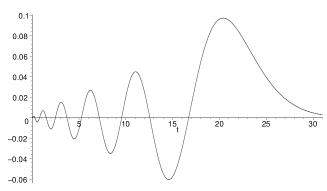
Figure 4. Graphs of $\gamma_{11}$ for $\alpha=1$ and $\gamma_{11.5}$ $\alpha=2$

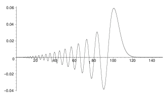
Figure 5. Graphs of $\gamma_{52.5}$ and $\gamma_{102.5}$ for $\alpha=4$

4. Speed of approximation

4.1. The strategy

We return for a moment to the general setting of Section 2. We saw that a signal in ${\mathcal{H}}_{\varpi}$ can be written a the sum of a series $\sum_{n\in{\mathbb{Z}}}a_{n}\,\gamma_{n}$, which converges in norm within this Hilbert space.

In practice, and especially in a sampling framework, it is important both to secure convergence and to evaluate approximation rates in various norms such as $L_{\infty}$ and $L^{2}$ in addition to ${\mathcal{H}}_{\varpi}$. As we shall see, it is possible to recover uniform or $L^{2}$ estimates from the ${\mathcal{H}}_{\varpi}$-norm. Indeed, if the weight $\varpi$ is bounded from below by a positive constant, then the ${\mathcal{H}}_{\varpi}$ convergence implies the $L^{2}$ one and if $\int_{|\omega|>1}\varpi(\omega)^{-1}\,\mathrm{d}\omega<+\infty$, it implies uniform convergence. Moreover, if $\int_{|\omega|>1}\frac{|\omega|^{2k}}{\varpi(\omega)}\,\mathrm{d}\omega<+\infty$, then one has uniform convergence of the derivatives up to order $k$.

As a consequence, estimates of the uniform norm or the $L^{2}$ norm of $\mbox{err}_{N}=\sum_{|n|>N}a_{n}\gamma_{n}$ may be deduced from estimates $s_{N}=\sum_{|n|>N}|a_{n}|^{2}$. But the coefficients $a_{n}$ are nothing but the Fourier coefficient of the warped function ${\mathcal{T}}^{\psi,\chi}(X)$ with respect to the orthonormal basis $\{e_{n}\}$. Our strategy is thus simple: Choose for $\{e_{n}\}$ the trigonometric system, and then make use of classical properties of the Fourier coefficients. For instance, if a $L^{1}$ function on the torus is Hölder $h$ in the $L^{1}$ norm, one has $a_{n}={\mathcal{O}}\left(|n|^{-h}\right)$. In this way one is able to get the speed of convergence of the series for functions $X$ such that the warped signal $\widehat{X}\circ\varphi(u)\,\varphi^{\prime}(u)^{\frac{\alpha+1}{2}}$ extends as a $|I|$-periodic $C^{k}$-function.

In order to achieve this program and to be able to give tractable conditions on the signal under processing, one has to particularize the warping function. The case studied in Section 3 gives rise to explicit formulae, but it will appear that there are not enough free parameters. This is why we introduce more general a family of warping operators.

4.2. Another family of warping operators

Inspired by the case $\varphi(u)=\tan(u)$ treated above, we explore a more general setting where $\psi$ and $\chi$ are given by

(4.1) $$\psi(\xi)=c_{1}\int_{0}^{\xi}\frac{\mathrm{d}v}{(1+v^{2})^{\beta}}\text{\quad and\quad}\chi=(\varphi^{\prime})^{\frac{\alpha+1}{2}},$$

where $\beta>1/2$ and $c_{1}^{-1}=\frac{2}{\pi}\int_{0}^{+\infty}\frac{\mathrm{d}v}{(1+v^{2})^{\beta}}$ (as previously, $\varphi$ stands for the function reciprocal to $\psi$).

Note that if $\beta\leq\frac{1}{2}$ could be of interest, but is not studied in this work.

We have

(4.2) $$\varphi^{\prime}\circ\psi(\omega)=1/\psi^{\prime}(\omega)=c_{1}^{-1}(1+\omega^{2})^{\beta}.$$

As a consequence, ${\mathcal{H}_{\varpi}}$ is the usual Sobolev space of order $\alpha\beta$

$${\mathcal{H}}^{\alpha\beta}=\left\{X\in\mathcal{S}^{\prime}({\mathbb{R}})\text{ such that }\int_{\mathbb{R}}|\widehat{X}(\omega)|^{2}(1+\omega^{2})^{\alpha\beta}\mathrm{d}f<+\infty\right\}.$$

It can be checked that, for any $k\geq 0$,

(4.3) $$\frac{\mathrm{d}^{k+1}\psi}{\mathrm{d}\omega^{k+1}}(\omega)\sim\frac{c_{k}}{\omega^{2\beta+k}}$$

for large $|\omega|$.

Moreover, when $\omega\to+\infty$,

(4.4) $$\psi(\omega)=\frac{\pi}{2}-\frac{c_{3}}{\omega^{2\beta-1}}+\mbox{{\rm\small o}}\left(\frac{1}{\omega^{2\beta-1}}\right).$$

So, when $u\rightarrow\frac{\pi}{2}$,

(4.5) $$\varphi(u)\sim\left(\frac{\pi}{2}-u\right)^{-\frac{1}{2\beta-1}}.$$

Finally, using (4.3) and (4.5), it is easily proved that for all $k\geq 0$

(4.6) $$\varphi^{(k)}(u)\sim\left(\frac{\pi}{2}-u\right)^{-\frac{1}{2\beta-1}-k}.$$

We are now ready to define a family of functional spaces for which speed of convergence results are easily obtained.

Definition 10.

If $m\in{\mathbb{N}}$ and $\mu>0$, let ${\mathcal{W}}_{m}^{\mu}$ denote the space of functions $X\in\mathcal{S}^{\prime}({\mathbb{R}})$ such that

1. $\widehat{X}$ is $m$ times differentiable

2. if $0\leq k\leq m$ then $|\widehat{X}^{(k)}(\omega)|={\mathcal{O}}\left(|\omega|^{-(\mu+k)}\right)$ for large $|\omega|$.

Condition 2 obviously entails that ${\mathcal{W}}_{m}^{\mu}$ is a subspace of ${\mathcal{H}}^{\mu-\frac{1}{2}-\varepsilon}$ for all positive $\varepsilon$. Condition 1 imposes some smoothness on $\widehat{X}$. Functions in ${\mathcal{W}}_{m}^{\mu}$ are thus sufficiently “well-behaved” both in the time and frequency domains.

Proposition 11.

Let $m$ be a positive integer and $\alpha$, $\beta$, and $\mu$ be nonnegative real numbers satisfying $\beta>\frac{1}{2}$, $2\alpha\beta<2\mu-1$, and $X\in{\mathcal{W}}_{m}^{\mu}$. Let $\sum_{n\in{\mathbb{Z}}|}a_{n}\gamma_{n}$ be the $(\alpha,\beta)$-development of an $X\in{\mathcal{H}}^{\alpha\beta}$. Then

• $$\left\|\sum_{|n|>N}a_{n}\gamma_{n}\right\|_{2}={\mathcal{O}}\left(N^{\frac{1}{2}-\varkappa}\right),$$

• if moreover $\alpha\beta>\frac{1}{2}$,

  $$\left\|\sum_{|n|\geq N}a_{n}\gamma_{n}\right\|_{\infty}={\mathcal{O}}\left(N^{\frac{1}{2}-\varkappa}\right),$$

where $\varkappa=\min\left\{m,\frac{\mu-\alpha\beta-\beta}{2\beta-1}\right\}$.

Proof.

Since $\alpha\beta<\mu-\frac{1}{2}$, we have $X\in{\mathcal{H}}^{\alpha\beta}$. Consider the warped function $g(u)=\widehat{X}\circ\varphi(u)\varphi^{\prime}(u)^{\frac{\alpha+1}{2}}$. Due to 4.5 and to the fact $X\in{\mathcal{H}}_{m}^{\mu}$, for all $k\leq m$, one has,

$$g^{(k)}(u)={\mathcal{O}}\left(\left(\frac{\pi}{2}-|u|\right)^{\frac{\mu-\beta(\alpha+1)}{2\beta-1}-k}\right)$$

when $u\rightarrow\pm\frac{\pi}{2}$. This means that $g$ extends as a $\pi$-periodic $\Lambda_{\alpha}$-function (see [11]). It results the estimate $a_{n}={\mathcal{O}}\left(|n|^{-\varkappa}\right)$ for its Fourier coefficients. This implies $\left\|\sum_{|n|>N}a_{n}\gamma_{n}\right\|_{{\mathcal{H}}^{\alpha\beta}}^{2}=\sum_{|n|>N}|a_{n}|^{2}={\mathcal{O}}\left(N^{1-2\varkappa}\right)$, from which the conclusions easily follow.. ∎

Theorem 12.

Let $X$ belong to ${\mathcal{W}}_{m}^{\mu}$. Then one has the following facts.

1. If $\mu>1$, there exist $\alpha$ and $\beta$ such that $||X-X_{N}||_{\infty}={\mathcal{O}}\left(\frac{1}{N^{m-\frac{1}{2}}}\right)$.

2. If $\mu>1/2$, there exist $\alpha$ and $\beta$ such that $||X-X_{N}||_{2}={\mathcal{O}}\left(\frac{1}{N^{m-\frac{1}{2}}}\right)$.

Where, in both cases, $X_{N}$ stands for the partial sum $\sum_{|n|\leq N}a_{n}\gamma_{n}$ of the corresponding ($\alpha,\beta$)-warping expansion of $X$.

Proof.

If suffices to check that, given $m$ and $\mu$ fulfilling the hypotheses, one can find $\alpha$ and $\beta$ satisfying the constraints in Proposition • ‣ 11. ∎

Figure 6. Explanation of theorem 12.

The following corollary shows that functions with very regular Fourier transforms can be approximated with any prescribed polynomial speed.

Corollary 13.

Let $X$ belong to ${\mathcal{W}}_{\infty}^{\mu}$, with $\mu>1$ (rep. $\mu>1/2$). Then, for all $\gamma>0$, there exists a warping operator such that $||X-X_{N}||_{\infty}=\mbox{{\rm\small o}}\left(N^{-\gamma}\right)$ (resp. $||X-X_{N}||_{2}=\mbox{{\rm\small o}}\left(N^{-\gamma}\right)$).

4.3. Comparison with WKS sampling

Introductory remarks

In this section, we deal with the practical aspects of our warping method. We showed that, provided $X$ belongs to a given (large) class of signals, excellent approximations of $X$ can be obtained by keeping a finite number of terms in the sum $\sum_{n\in{\mathbb{Z}}}\langle X,\gamma_{n}\rangle_{H_{\varpi}}\gamma_{n}$.

Now, we are going to compare the warping with the classical sampling method based on low-pass filtering.

Assume we are given a analog signal $X$, which needs to be digitized for purposes of storing, transmitting, or digital processing. A crude application of Shannon sampling consists in the following steps:

1. to fix a sampling frequency $\omega_{0}$,

2. to low-pass $X$, i.e., to compute the convolution $X_{l}=X*g$, where $\widehat{g}={\bf 1}_{[-\omega_{0}/2\pi,\omega_{0}/2\pi]}$,

3. to approximate $X(t)$ by $\widetilde{X}_{l}(t)=\sum_{|n|\leq N_{s}}X_{l}(n)\operatorname{sinc}\frac{t-\frac{2\pi n}{\omega_{0}}}{\frac{2\pi}{\omega_{0}}}$.

This procedure generates two kinds of errors. The first one is due to low-pass filtering. The second one arises in step 3, because of the truncation of the series. Such a truncation is unavoidable since obviously one can access only finitely many samples in practice.

The warping procedure for digitizing signals proceeds as follows:

1. to fix a natural number $N_{w}$,

2. to compute the scalar products $\langle X,\gamma_{k}\rangle_{H_{\varpi}}$ for $n=-N_{w}\ldots N_{w}$,

3. to approximate $X(t)$ by $\sum_{n=-N_{w}}^{N_{w}}\langle X,\gamma_{n}\rangle_{H_{\varpi}}\gamma_{n}$.

Again two kinds of errors are made. The first one lies in the estimation of the scalar products. As previously, the second one is a consequence of keeping finitely many terms in the sum in step 3. In this work, we shall assume that the first kind of error is negligible with respect to the second one. Indeed, when $\varphi=\tan$, we obtained explicit expressions for the $\gamma_{n}$. In this case, it is not too hard to devise a sufficiently precise numerical approximation scheme using these expressions. In more general cases, the scalar products may be harder to compute. We plan to investigate numerical quadrature schemes for solving this important problem in a forthcoming work.

If the WKS and warping procedures are to be compared, it is fair to set $N_{s}=N_{w}$, henceforth denoted $N$. One then needs to select a value for $\omega_{0}$. Obviously, in the case where $X$ is not bandlimited, one would like to take $\omega_{0}$ as large as possible. However, in practice, one passes from the “time domain” to the “Fourier domain” through the Fast Fourier Transform. As a consequence, it does not make sense to choose $\omega_{0}$ larger than $N$.

4.3.1. Worst case comparison

It is not easy to compare the error made in approximating an arbitrary function through WKS sampling and warping. In order to obtain tractable results, we shall rather compare the worst case approximations in both situations.

More precisely, for a function $X$ in ${\mathcal{W}}_{m}^{\mu}$, the $L^{\infty}({\mathbb{R}})$ error when considering $N$ terms in the cardinal series and setting $\omega_{0}=N$ is of order not larger than

$$\int_{N}^{+\infty}\frac{\mathrm{d}\omega}{\omega^{\mu}}=\frac{1}{N^{\mu-1}}$$

whereas the $L^{2}({\mathbb{R}})$ error is of order not larger than

$$\frac{1}{N^{\mu-\frac{1}{2}}}.$$

These errors only depend on $\mu$, which is in contrast to what happens for the errors in the warping method.

Let us introduce the ratios of the worst cases errors corresponding to the warping and WKS sampling:

$$\rho_{\infty}(N)=\frac{N^{\varkappa-\frac{1}{2}}}{N^{\mu-1}}=N^{\varkappa+\frac{1}{2}-\mu}$$

$$\rho_{2}(N)=\frac{N^{\varkappa-\frac{1}{2}}}{N^{\mu-\frac{1}{2}}}=N^{\varkappa-\mu}.$$

The following proposition gives conditions on $\alpha,\beta,m$, and $\mu$ under which warping is preferable to low-pass filtering, i.e., yields faster convergence rates.

Proposition 14 (Comparison in $L_{2}$ and $L_{\infty}$).

Let $m$ be a positive integer and $\alpha$, $\beta$, and $\mu$ be nonnegative real numbers satisfying $\beta>\frac{1}{2}$, $0<\alpha\beta<\mu-\frac{1}{2}$, $2\mu(1-\beta)>\alpha\beta+\beta$, and $m>\mu$. Then, the ratio of the worst cases errors for a function in ${\mathcal{W}}_{m}^{\mu}$ sampled through the WKS theorem and through the warping operator with parameters ($\alpha,\beta$) are such that:

• $\lim_{N\to\infty}\rho_{2}=+\infty$, and,

• if $\alpha\beta>\frac{1}{2}$, $\lim_{N\to\infty}\rho_{\infty}=+\infty$.

Note that the conditions set on the parameters imply that $\mu>1$ for the $L_{\infty}$ error, and that $\mu>\frac{1}{2}$ for the $L_{2}$ error. Accordingly, $m$ must be at least 2 in the $L_{\infty}$ case, and at least 1 in the $L_{2}$ case: In order for the warping procedure to be better than the WKS one in, e.g., the $L_{2}$ sense, $\widehat{X}$ must thus be at least once differentiable with a derivative decaying faster than $\frac{1}{\omega^{3/2}}$. For instance, functions in ${\mathcal{W}}_{1}^{1/4}$ are advantageously sampled through warping (in the $L_{2}$ sense) with, e.g., $\beta=\frac{11}{20}-\varepsilon,\alpha\beta=\frac{1}{8},0<\varepsilon<\frac{1}{20}$.

Proof.

This results from Proposition • ‣ 11. ∎

5. Numerical experiments

We now present results of numerical experiments that illustrate the behavior of the warping method for approximating certain functions. We compare it to the quality of approximation obtained using the classical WKS sampling framework.

5.1. Methodology

We give ourselves a series of functions to be analyzed, and then reconstructed using the WKS sampling algorithm, and our method. We focus on the case $\alpha=\beta=1$, i.e., $\psi=\arctan$ and the space of approximation is ${\mathcal{H}}^{1}$.

The full procedure is defined as:

• In the classical sampling approach, each signal $X(t)$ is low-pass filtered at frequency $2\pi N$, then sampled at the Nyquist frequency (the sampling pace is thus $\frac{1}{N}$). Finally, it is reconstructed as $\widetilde{X}_{l}(t)$ using the cardinal series. In our examples, all signals compactly supported (i.e., time limited) on $[0,10]$, and therefore the summation is finite (there are $10N$ terms).

• For our algorithm, each signal is decomposed into the system $\{\gamma_{n}\}_{0\leq n\leq N-1}$ and is then reconstructed as

  $$\widetilde{X}_{w}(t)=\sum_{n=0}^{N-1}c_{n}\gamma_{n}(t)$$

• In each case we compute the uniform error, the $L^{2}$ error and the $H_{1}$ error. All errors are relative errors:

  $$E=\frac{\|X-\widetilde{X}\|}{\|X\|}$$

• This process is repeated for several values of $N$, typically $N=1,...,78$.

This procedure allows us to study and compare the quality of approximation of both methods in terms of different metrics. Notice that in each case, the number of terms retained to reconstruct $X$ is $N$. This is the cost of compression in terms of information quantity.

5.2. Practical implementation

Concerning the WKS sampling, functions must be low-pass filtered. From a practical point of view, two cases may be distinguished:

• Either the filtered version of $X$ has an analytic form, as is the case for the Riemann function

  $$R_{s}(t)=\sum_{k\geq 0}\frac{\sin(n^{s}t)}{n^{s}}$$

  In this case, bandlimiting is equivalent to truncating the sum, and the samples can be expressed in a closed form:

  $$\widetilde{X}_{l}(t_{k})=\sum_{0\leq k^{s}\leq N}\frac{\sin(n^{s}t_{k})}{n^{s}}$$

  The expression of the samples is then used to compute the cardinal series.

• Or there is no analytic form for the low-pass filtered version of $X$. In this case the samples must be approximated using a Discrete Fourier Transform (DFT). We must thus first simulate a "continuous" (i.e., non-sampled) version of the signal. This is achieved by means of a large sampling rate. More precisely, we first discretize the signal on $[0,10]$ with a regular grid of $10^{5}$ points. We then compute the DFT (via a Fast Fourier Transform, FFT) of this approximate "continuous" signal, low-pass filtered the Fourier transform and then we applied an inverse DFT.

As regards the implementation of the warping method, two types of quantities must be computed. First the functions $\gamma_{k}$, for $0\leq k\leq N-1$, and then the coefficients $c_{k}=\langle\widetilde{\gamma}_{k},f\rangle$. The latter are expressed as a duality product between the signal $X$ to be analyzed and the dual functions $\widetilde{\gamma}_{k}$.

We proceeded as follows: the functions $\gamma_{k}$ were pre-computed under Maple in a discretized form (sampled on a regular grid of gridspace equal to $10^{-3}$) using the analytic form given in section 3 for $\alpha=1$. For the dual functions $\widetilde{\gamma}_{k}$, it is a bit more complicated: they correspond to $\alpha=-1$ and their expression is given in section 3 as a sum of a Dirac mass and an analytic part. These two components must be separated. We pre-computed the analytic part under Maple (like for the $\gamma_{k}$) and $c_{k}$ was evaluated as the sum of the inner product of $f$ with the analytic part, plus a coefficient times $X(0)$ (corresponding to the duality product with the Dirac mass).

It is to be noted that the error can also be evaluated in other Sobolev metrics, say in $H_{\nu}$, where $\nu>0$. In this case, one has to work in the Fourier domain and therefore use an FFT.

5.3. Results

We consider four examples of functions with increasing complexity. In each case, we display four curves. The first one is a superposition of the original function with the approximations yielded by both the WKS and the warping methods with a single, large, value of $N$. The three other graphs describe the evolutions of the $L^{\infty},L^{2}$ and $H^{1}$ errors of both approximation methods as a function of $N$.

Cauchy Probability Distribution

Our first test deals with a smooth function, namely the Cauchy probability distribution $\frac{1}{1+t^{2}}$. Since we consider the restriction of this function to $[0,10]$, we however introduce a discontinuity at the endpoints, i.e., the values at 0 and 10 differ. The warping method appears extremely efficient when $N$ remains moderate (<30). Even for large values of $N$, this method remains superior to the WKS algorithm as the errors for the latter is larger (see figure 7). One reason for this is the above mentioned discontinuity: As a consequence, the WKS approximation is quite bad around the boundaries of the domain $[0,10]$, because in the sum many terms are missing. On the contrary, if one takes enough terms in the sum for the warping, the approximation is excellent around 0, and quite good at 10.

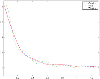
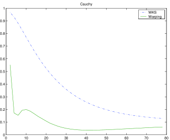
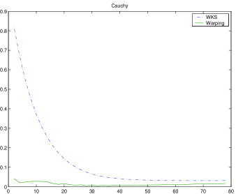
Figure 7. Approximations of $\frac{1}{1+t^{2}}$ for $N=78$ (upper left), uniform error as a function of $N$ (upper right), $L^{2}$ error (lower left) and $H_{1}$ error (lower right).

Chirp

We now consider a function with wild oscillations, the (modified) chirp $t\sin(\frac{1}{t})e^{-t}$, restricted to $[0,10]$. The exponential factor aims at getting an $H_{1}$ function that is numerically equal to 0 at $t=10$, so as not to penalize the WKS approximation with a boundary discontinuity. The two methods present similar performances, although there is a slight but noticeable gain of efficiency with the warping, as seen on figure 8.

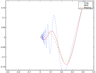
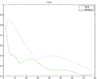
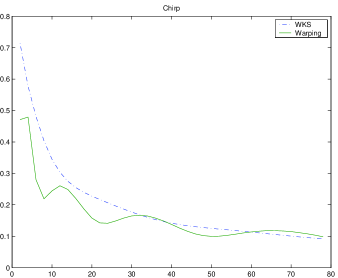
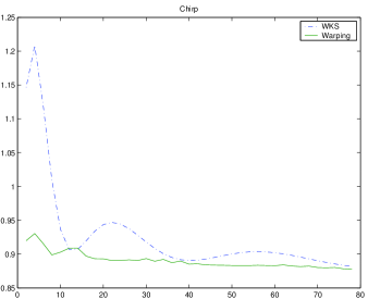
Figure 8. Approximations of $t\sin(\frac{1}{t})e^{-t}$ for $N=78$ (upper left), uniform error as a function of $N$ (upper right), $L^{2}$ error (lower left) and $H_{1}$ error (lower right).

Riemann function

We now focus on a function which is everywhere irregular and has a multifractal structure. The Riemann function is defined as

$$R_{s}(t)=\sum_{n\geq 0}\frac{\sin(n^{s}t)}{n^{s}}$$

In our numerical study, we took $s=1.8$, which guarantees that $R_{s}\in L^{2}$. As above, we analyze the restriction to $[0,10]$. The function is "numerically equal" to zero at $10$, thus there is no discontinuity at the endpoints.

The results are shown on figure 9. Clearly the warping method gives better results. In fact, the sine series defining $R_{s}$ being lacunary, the WKS sampling method will not capture sine waves for increasingly long ranges of values of $N$, and consequently, for $(n-1)^{s}\leq N<n^{s}$, the WKS approximation $\widetilde{X}_{l}$ remains the same (see the steps on figure 9). On the contrary, the warping approximation improves steadily as $N$ grows.

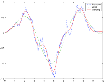
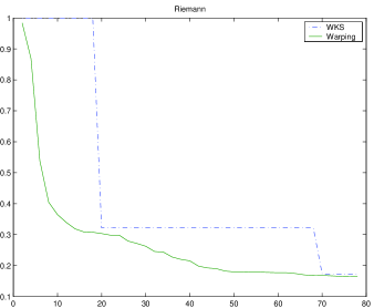
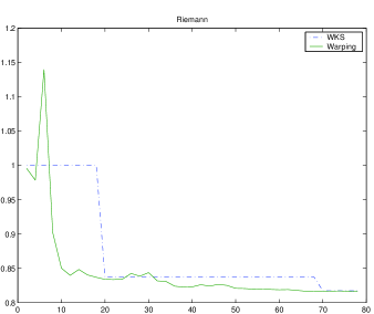
Figure 9. Approximations of the Riemann function $R_{s}$ for $N=50$ (upper left), uniform error as a function of $N$ (upper right), $L^{2}$ error (lower left) and $H_{1}$ error (lower right).

5.3.1. Weierstrass function

The same phenomenon occurs for the (modified) Weierstrass function

$$W_{h}(t)=e^{-\frac{t^{2}}{\sigma^{2}}}\sum_{k\geq 0}\lambda^{-kh}\sin(\lambda^{k}t)$$

where $h>0$, $\lambda\geq 2$ and $\sigma>0$. This function has everywhere a Hölder exponent equal to $h$. The Gaussian factor allows to obtain an $L^{2}$ function which is numerically 0 at $t=10$, and with a Fourier transform:

$$\widehat{W}_{h}(\omega)=\sum_{k\geq 0}2^{-kh}e^{-\frac{(\omega-2\pi 2^{k})^{2}\sigma^{2}}{2}}$$

so that $W_{h}$ belongs to the spaces ${\mathcal{W}}_{m}^{\mu}$ for all $0<m<h$ and $\mu\leq h-m$.

From the results in Section 4, warping-based sampling will yield a better approximation than WKS sampling as soon as $h>3/2$, with the following choice of the parameters:

$\alpha\beta=h-\frac{3}{2}-2\varepsilon$, with $2\varepsilon<h-3/2$,      $\frac{1}{2}<\beta<\frac{1}{2}+\frac{\varepsilon}{2h-1-2\varepsilon}$    (when $m=1$).

In order to show that the warping method may outperform WKS sampling also for functions that do not belong to a space ${\mathcal{W}}_{m}^{\mu}$, we studied numerically the case $\lambda=2,h=0.8$ and $\sigma=1$. The results are on figure 10. Again, the sine series is lacunary and the WKS error remains constant on large ranges of values of $N$, resulting in strongly different behaviors for the WKS and warping approximations.

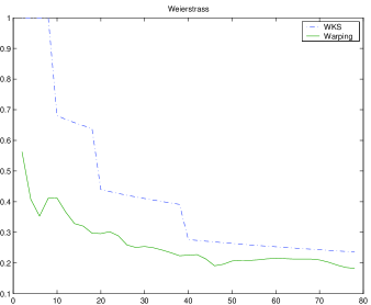
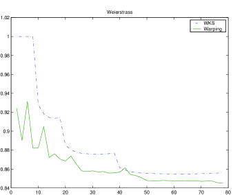
Figure 10. Approximations of the Weierstrass function $W_{h}(t)$ for $N=30$ (upper left), uniform error as a function of $N$ (upper right), $L^{2}$ error (lower left) and $H_{1}$ error (lower right).

We conclude this section by mentioning how to treat the case where $\alpha\neq 1$ or $\beta\neq 1$. This is necessary in order to process with maximum accuracy functions in spaces ${\mathcal{W}}_{m}^{\mu}$ with various values of $m$ and $\mu$.

First, if $\alpha\neq 1$ and $\beta=1$, we can use the expressions for $\gamma_{k}$ given in section 3, and proceed exactly as for the case $\alpha=1$ (i.e., $\psi=\arctan$), that is by pre-computing $\gamma_{k}$ and $\widetilde{\gamma}_{k}$. Of course, for the dual functions, more Dirac masses come into play, and computing the inner product involves the evaluation of more derivatives of $X$ at 0. If $\beta\neq 1$, the warping function changes, and things get more complicated. There is however a situation where analytical computations are feasible: Indeed, when $\beta$ is an odd integer, it is possible to compute the expression of $\gamma_{k}$. Therefore one can proceed as in the case $\beta=1$. In general, there will be no closed form expression for $\gamma_{k}$. These functions should then be approximated using their expression in the Fourier domain. More precisely, one can pre-compute the warping function $\psi$ on a grid:

$$\psi(\omega)=c\int_{0}^{\omega}\frac{dv}{(1+v^{2\beta})}$$

and use this to tabulate

$$\widehat{\gamma}_{k}(\omega)=\sqrt{\psi^{\prime}(\omega)}e^{2i\pi k\psi(w)}$$

Then one can use an inverse DFT to obtain an approximation of $\gamma_{k}$. Likewise, the coefficients $c_{k}=\langle\widetilde{\gamma}_{k},X\rangle=\langle\widehat{\widetilde{\gamma}}_{k},\widehat{X}\rangle$ must be computed in the Fourier domain.

References

[1] H.G. Feichtinger and K. Gröchenig, Theory
and Practice of Irregular Sampling. In "Wavelets: Mathematics and
Applications,” J. Benedetto and M. Frazier M., editors, CRC Press,
1993, 305–363.
[2] I.S. Gradshteyn and I.M. Ryzhik, Table of
integrals,series, and products. Academic Press, 2000. ISBN
0-12-294757-6.
[3] Abdul J. Jerri, Integral and discrete
transforms with applications and error analysis. Monographs and
Textbooks in Pure and Applied Mathematics, 1992.
[4] V.A. Kotel’nikov, On the transmission
capacity of ether and wire in electrocommunications. Izd. Red. Upr. Svyazzi RKKA (Moscow), 1933.
[5] W. Magnus and F. Oberhettinger, Formulas and
theorems for the functions of mathematical physics. Chelsea
publishing company.
[6] R. J. Marks Introduction to Shannon Sampling
and Interpolation Theory. Springer Texts in Electrical Engineering,
New York, Berlin: Springer,1991
[7] Advanced topics in Shannon sampling and
interpolation theory. R. J. Marks (Ed.) Springer Texts in
Electrical Engineering, New York, Berlin: Springer,1993.
[8] C.E. Shannon, Communication in the presence
of noise. in Proc. IRE, vol. 37, 1949, 10–21.
[9] G. Szegö, Orthogonal polynomials.
American Mathematical Society Colloquium Publications, volume XXIII,
fourth edition, 1978. ISBN 0-8218-1023-5.
[10] J.M. Whittaker, The Fourier theory of the
cardinal functions. in Proc. Math. Soc. Edinburgh, vol. 1,
1929, 169–176.
[11] A. Zygmund, Trigonometric series.
Cambridge University Press, Cambridge, 1935.