Linear and non-linear Modified Gravity forecasts with future surveys

Abstract

Modified Gravity theories generally affect the Poisson equation and the gravitational slip (effective anisotropic stress) in an observable way, that can be parameterized by two generic functions ($\eta$ and $\mu$) of time and space. We bin the time dependence of these functions in redshift and present forecasts on each bin for future surveys like Euclid. We consider both Galaxy Clustering and Weak Lensing surveys, showing the impact of the non-linear regime, treated with two different semi-analytical approximations. In addition to these future observables, we use a prior covariance matrix derived from the Planck observations of the Cosmic Microwave Background. Our results show that $\eta$ and $\mu$ in different redshift bins are significantly correlated, but including non-linear scales reduces or even eliminates the correlation, breaking the degeneracy between Modified Gravity parameters and the overall amplitude of the matter power spectrum. We further decorrelate parameters with a Zero-phase Component Analysis and identify which combinations of the Modified Gravity parameter amplitudes, in different redshift bins, are best constrained by future surveys. We also extend the analysis to two particular parameterizations of the time evolution of $\mu$ and $\eta$ and consider, in addition to Euclid, also SKA1, SKA2, DESI: we find in this case that future surveys will be able to constrain the current values of $\eta$ and $\mu$ at the 2-5% level when using only linear scales (wavevector k < 0.15 h/Mpc), depending on the specific time parameterization; sensitivity improves to about $1\%$ when non-linearities are included.

I Introduction

Future large scale structure surveys will be able to measure with percent precision the parameters governing the evolution of matter perturbations. While we have the tools to investigate the standard model, the next challenge is to be able to compare those data with cosmologies that go beyond General Relativity, in order to test whether a fluid component like Dark Energy or similarly a Modified Gravity scenario can better fit the data. On the theoretical side, while many Modified Gravity models are still allowed by type Ia supernova (SNIa) and Cosmic Microwave Background (CMB) data Planck Collaboration et al. (2016); structure formation can help us to distinguish among them and the standard scenario, thanks to their signatures on the matter power spectrum, in the linear and mildly non-linear regimes (for some examples of forecasts, see Amendola and others (2013); Casas et al. (2015); Bielefeld et al. (2014)).

The evolution of matter perturbations can be fully described by two generic functions of time and space Kunz (2012); Amendola et al. (2013), which can be measured via Galaxy Clustering and Weak Lensing surveys. In this work we want to forecast how well we can measure those functions, in different redshift bins.

While any two independent functions of the gravitational potentials would do, we follow the notation of Planck Collaboration et al. (2016) and consider $\mu$ and $\eta$: the first modifies the Poisson equation for $\Psi$ while the second is equal to the ratio of the gravitational potentials (and is therefore also a direct observable Amendola et al. (2013)). We will consider forecasts for the planned surveys Euclid, SKA1 and SKA2 and a subset of DESI, DESI-ELG, using as priors the constraints from recent Planck data (see also Alonso et al. (2016); Hojjati et al. (2012); Baker and Bull (2015); Bull (2015); Gleyzes et al. (2016) for previous works that address forecasts in Modified Gravity.

In section II we define $\mu$ and $\eta$ and parameterize them in three different ways. First, in a general manner, we let these functions vary freely in different redshift bins. Complementarily, we also consider two specific parameterizations of the time evolution proposed in Planck Collaboration et al. (2016). Here, we also specify the fiducial values of our cosmology for each of the parameterizations considered. Section III discusses our treatment for the linear and mildly non-linear regime. Linear spectra are obtained from a modified Boltzmann code Hojjati et al. (2011); the mild non-linear regime (up to k $\sim$ 0.5 h/Mpc) compares two methods to emulate the non-linear power spectrum: the commonly used Halofit Smith et al. (2003); Takahashi et al. (2012), and a semi-analytic prescription to model the screening mechanisms present in Modified Gravity models Hu and Sawicki (2007). In section IV we explain the method used to produce the Fisher forecasts both for Weak Lensing and Galaxy Clustering. We explain how we compute and add the CMB Planck priors to our Fisher matrices. Section V discusses the results obtained for the redshift binned parameterization both for Galaxy Clustering and for Weak Lensing in the linear and non-linear cases. We describe our method to decorrelate the errors in section V.4. The results for the other two time parameterizations are instead discussed in sections VI.1 and VI.2, both for Weak Lensing and Galaxy Clustering in the linear and mildly non-linear regimes. To test the effect of our non-linear prescription, we show in section VI.3 the impact of different choices of the non-linear prescription parameters on the cosmological parameter estimation.

II Parameterizing Modified Gravity

In linear perturbation theory, scalar, vector and tensor perturbations do not mix, which allows us to consider only the scalar perturbations in this paper. We work in the conformal Newtonian gauge, with the line element given by

$$ds^{2}=-(1+2\Psi)dt^{2}+a^{2}(1-2\Phi)dx^{2}\,\,\,.$$ (1)

Here $\Phi$ and $\Psi$ are two functions of time and scale that coincide with the gauge-invariant Bardeen potentials in the Newtonian gauge.

In theories with extra degrees of freedom (Dark Energy, DE) or modifications of General Relativity (MG) the normal linear perturbation equations are no longer valid, so that for a given matter source the values of $\Phi$ and $\Psi$ will differ from their usual values. We can parameterize this change generally with the help of two new functions that encode the modifications. Many different choices are possible and have been adopted in the literature, see e.g. Planck Collaboration et al. (2016) for a limited overview. In this paper we introduce the two functions through a gravitational slip (leading to $\Phi\neq\Psi$ also at linear order and for pure cold dark matter) and as a modification of the Poisson equation for $\Psi$,

$$-k^{2}\Psi(a,k) \equiv 4\pi Ga^{2}\mu(a,k)\rho(a)\delta(a,k)\,\,\,;$$ (2)

$$\eta(a,k) \equiv \Phi(a,k)/\Psi(a,k)\,\,\,.$$ (3)

These expressions define $\mu$ and $\eta$. Here $\rho(a)$ is the average dark matter density and $\delta(a,k)$ the comoving matter density contrast – we will neglect relativistic particles and radiation as we are only interested in modeling the perturbation behaviour at late times. In that situation, $\eta$, which is effectively an observable Amendola et al. (2013), is closely related to modifications of GR Saltas et al. (2014); Sawicki et al. (2016), while $\mu$ encodes for example deviations in gravitational clustering, especially in redshift-space distortions as non-relativistic particles are accelerated by the gradient of $\Psi$.

When considering Weak Lensing observations then it is also natural to parameterize deviations in the lensing or Weyl potential $\Phi+\Psi$, since it is this combination that affects null-geodesics (relativistic particles). To this end we introduce a function $\Sigma(t,k)$ so that

$$-k^{2}(\Phi(a,k)+\Psi(a,k))\equiv 8\pi Ga^{2}\Sigma(a,k)\rho(a)\delta(a,k)\,\,\,.$$ (4)

Since metric perturbations are fully specified by two functions of time and scale, $\Sigma$ is not independent from $\mu$ and $\eta$, and can be obtained from the latter as follows:

$$\Sigma(a,k)=(\mu(a,k)/2)(1+\eta(a,k))\,\,\,.$$ (5)

Throughout this work, we will denote the standard Lambda-Cold-Dark-Matter ($\Lambda$CDM) model, defined through the Einstein-Hilbert action with a cosmological constant, simply as GR. For this case we have that $\mu=\eta=\Sigma=1$. All other cases in which these functions are not unity will be labeled as Modified Gravity (MG) models.

Using effective quantities like $\mu$ and $\eta$ has the advantage that they are able to model any deviations of the perturbation behaviour from $\Lambda$CDM expectations, they are relatively close to observations, and they can also be related to other commonly used parameterization Pogosian et al. (2010) On the other hand, they are not easy to map to an action (as opposed to approaches like effective field theories that are based on an explicit action) and in addition they contain so much freedom that we normally restrict their parameterisation to a subset of possible functions.

This has however the disadvantage of loosing generality and making our constraints on $\mu$ and $\eta$ parameterization-dependent. In this paper, we prefer to complement specific choices of parameterizations adopted in the literature (we will use the choice made in Planck Collaboration et al. (2016)) with a more general approach: we will bin the functions $\mu(a)$ and $\eta(a)$ in redshift bins with index $i$ and we will treat each $\mu_{i}$ and $\eta_{i}$ as independent parameters in our forecast; we will then apply a variation of Principal Component Analysis (PCA), called Zero-phase Component Analysis (ZCA). This approach has been taken previously in the literature by Hojjati et al. (2012), where they bin $\mu$ and $\eta$ in several redshift and $k$-$scale$ bins together with a binning of $w(z)$ and cross correlate large scale structure observations with CMB temperature, E-modes and polarization data together with Integrated Sachs-Wolfe (ISW) observations to forecast the sensitivity of future surveys to modifications in $\mu$ and $\eta$. In the present work, we will neglect a possible $k$-dependence, we will focus on Galaxy Clustering (GC) and weak lensing (WL) surveys and we will show that there are important differences between the linear and non-linear cases; including the non-linear regime generally reduces correlations among the cosmological parameters. In the remainder of this section we will introduce the parameterizations that we will use.

II.1 Parameterizing gravitational potentials in discrete redshift bins

As a first approach we neglect scale dependence and bin the time evolution of the functions $\mu$ and $\eta$ without specifying any parameterized evolution. To this purpose we divide the redshift range $0\leq z\leq 3$ in 6 redshift bins and we consider the values $\mu(z_{i})$ and $\eta(z_{i})$ at the right limiting redshift $z_{i}$ of each bin as free parameters, thus with the $i$ index spanning the values $\{0.5,1.0,1.5,2.0,2.5,3.0\}$. The first bin is assumed to have a constant value, coinciding with the one at $z_{1}=0.5$, i.e. $\mu(z<0.5)=\mu(z_{1})$ and $\eta(z<0.5)=\eta(z_{1})$. The $\mu(z)$ function (and analogously $\eta(z)$) is then reconstructed as

$$\mu(z)=\mu(z_{1})+\sum_{i=1}^{N-1}{\frac{\mu(z_{i+1})-\mu(z_{i})}{2}\left[1+\tanh{\left(s\frac{z-z_{i+1}}{z_{i+1}-z_{i}}\right)}\right]},$$ (6)

where $s=10$ is a smoothing parameter and $N$ is the number of binned values. We assume that both $\mu$ and $\eta$ reach the GR limit at high redshifts: to realize this, the last $\mu(z_{6})$ and $\eta(z_{6})$ values assume the standard $\Lambda\mathrm{CDM}$ value $\mu=\eta=1$ and both functions are kept constant at higher redshifts $z>3$.

Similarly, the derivatives of these functions are obtained by computing

$$\mu^{\prime}({\bar{z}_{j}})=\frac{\mu(z_{i+1})-\mu(z_{i})}{z_{i+1}-z_{i}},$$ (7)

with $\bar{z}_{j}=(z_{i+1}+z_{i})/2$, using the same $\tanh(x)$ smoothing function:

$$\frac{d\mu(z)}{dz}=\mu^{\prime}(\bar{z}_{1})+\sum_{j=1}^{N-2}{\frac{\mu^{\prime}(\bar{z}_{j+1})-\mu^{\prime}(\bar{z}_{j})}{2}\left[1+\tanh{\left(s\frac{z-\bar{z}_{j+1}}{\bar{z}_{j+1}-\bar{z}_{j}}\right)}\right]}\,\,\,.$$ (8)

In particular we assume $\mu^{\prime}=\eta^{\prime}=0$ for $z<0.5$ and for $z>3$. We set the first five amplitudes of $\mu_{i}$ and $\eta_{i}$ as free parameters, thus the set we consider is: $\theta=\{\Omega_{m},\Omega_{b},h,\ln 10^{10}A_{s},n_{s},\{\mu_{i}\},\{\eta_{i}\}\}$, with $i$ an index going from 1 to 5. We take as fiducial cosmology the values shown in Tab. 1 columns 5 and 6. We only modify the evolution of perturbations and assume that the background expansion is well described by the standard $\Lambda$CDM expansion law for a flat universe with given values of $\Omega_{m}$, $\Omega_{b}$ and $h$.

II.2 Parameterizing gravitational potentials with simple smooth functions of the scale factor

As an alternative approach, we assume simple specific, time parameterizations for the $\mu$ and $\eta$ MG functions, adopting the ones used in the Planck analysis Planck Collaboration et al. (2016). We neglect here as well any scale dependence:

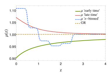
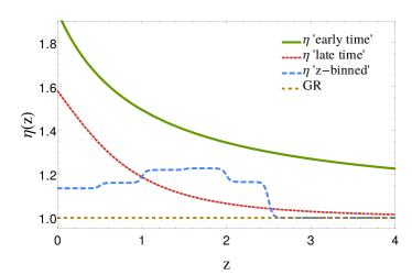
• a parameterization in which the time evolution is related to the dark energy density fraction, to which we refer as ‘late-time’ parameterization:

  $$\mu(a,k)\equiv 1+E_{{\rm 11}}\Omega_{{\rm DE}}(a)\,\,\,,$$ (9)

  $$\eta(a,k)\equiv 1+E_{{\rm 22}}\Omega_{{\rm DE}}(a)\,\,\,;$$ (10)

• a parameterization in which the time evolution is the simplest first order Taylor expansion of a general function of the scale factor $a$ (and closely resembles the $w_{0}-w_{a}$ parametrization for the equation of state of DE), referred to as ‘early-time’ parameterization, because it allows departures from GR also at high redshifts :

  $$\mu(a,k)\equiv 1+E_{{\rm 11}}+E_{{\rm 12}}(1-a)\,\,\,,$$ (11)

  $$\eta(a,k)\equiv 1+E_{{\rm 21}}+E_{{\rm 22}}(1-a)\,\,\,.$$ (12)

The late-time parameterization is forced to behave as GR ($\mu=\eta=1$) at high redshift when $\Omega_{{\rm DE}}(a)$ becomes negligible; the early time one allows more freedom as the amplitude of the deviations from GR do not necessarily reduce to zero at high redshifts. Both parameterizations have been used in Planck Collaboration et al. (2016). In Bull (2015); Gleyzes et al. (2016); Alonso et al. (2016) the authors used a similar time parameterization in which the Modified Gravity parameters depend on the time evolution of the dark energy fraction. In Bull (2015) an extra parameter accounts for a scale-dependent $\mu$: their treatment keeps $\eta$ (called $\gamma$ in their paper) fixed and equal to 1; it uses linear power spectra up to $k_{\mathrm{max}}(z)$ with $k_{\rm max}(z=0)=0.14$/Mpc $\approx$ 0.2 h/Mpc. In Gleyzes et al. (2016) the authors also use a combination of Galaxy Clustering, Weak Lensing and ISW cross-correlation to constrain Modified Gravity in the Effective Field Theory formalism Gubitosi et al. (2013). In Bellini et al. (2016) and Alonso et al. (2016) a similar parameterization was used to constrain the Horndeski functions Bellini and Sawicki (2014) with present data and future forecasts respectively, in the linear regime.

For the late-time parameterization, the set of free parameters we consider is: $\theta=\{\Omega_{m},\Omega_{b},h,\ln 10^{10}A_{s},n_{s},E_{11},E_{22}\}$, where $E_{11}$ and $E_{22}$ determine the amplitude of the variation with respect to $\Lambda\mathrm{CDM}$. As fiducial cosmology we use the values shown in Table 1, columns 1 and 2, i.e. the marginalized parameter values obtained fitting these models with recent Planck data; notice that these results differ slightly from the Planck analysis in Planck Collaboration et al. (2016) for the same parameterization, because we don’t consider here the effect of massive neutrinos.

For the early time parameterization we have $E_{11}$ and $E_{21}$ which determine the amplitude of the deviation from GR at present time ($a=0$) and 2 additional parameters ($E_{12},\ E_{22}$), which determine the time dependence of the $\mu(a)$ and $\eta(a)$ functions for earlier times. The fiducial values for this model, obtained from the Planck+BSH best fit is given in columns 3 and 4 of Table 1.

Late time		Early time		Redshift Binned
Parameter	Fiducial	Parameter	Fiducial	Parameter	Fiducial
$\Omega_{c}$	$0.254$	$\Omega_{c}$	$0.256$	$\Omega_{c}$	$0.254$
$\Omega_{b}$	$0.048$	$\Omega_{b}$	$0.048$	$\Omega_{b}$	$0.048$
$n_{s}$	$0.969$	$n_{s}$	$0.969$	$n_{s}$	$0.969$
$\ln 10^{10}A_{s}$	$3.063$	$\ln 10^{10}A_{s}$	$3.091$	$\ln 10^{10}A_{s}$	$3.057$
$h$	$0.682$	$h$	$0.682$	$h$	$0.682$
$E_{11}$	$0.100$	$E_{11}$	$-0.098$	$\mu_{1}$	$1.108$
$E_{22}$	$0.829$	$E_{12}$	$0.096$	$\mu_{2}$	$1.027$
		$E_{21}$	$0.940$	$\mu_{3}$	$0.973$
		$E_{22}$	$-0.894$	$\mu_{4}$	$0.952$
				$\mu_{5}$	$0.962$
				$\eta_{1}$	$1.135$
				$\eta_{2}$	$1.160$
				$\eta_{3}$	$1.219$
				$\eta_{4}$	$1.226$
				$\eta_{5}$	$1.164$

Table 1: Fiducial values for the Modified Gravity parameterizations and the redshift-binned model of $\mu$ and $\eta$ used in this work. The DE related parameterization contains two extra parameters $E_{11}$ and $E_{22}$ with respect to GR; the early-time parametrization depends on 4 extra parameters $E_{11},\,E_{12},\,E_{22}$ and $E_{21}$ with respect to GR; the redshift-binned model contains 10 extra parameters, corresponding to the amplitudes $\mu_{i}$ and $\eta_{i}$ in five redshift bins. In this work we will use alternatively and for simplicity the notation $\ell\mathcal{A}_{s}\equiv\ln(10^{10}A_{s})$. The fiducial values are obtained performing a Monte Carlo analysis of Planck+BAO+SNe+H₀ (BSH) data Planck Collaboration et al. (2016).

Figure 1: The Modified Gravity functions $\mu$ and $\eta$ as a function of redshift $z$ for each of the models considered in this work, evaluated at the fiducials specified inTable 1. In light long-dashed blue lines, the ‘redshift binned model’ (Eqns. 6-8). In short-dashed red lines the late-time parameterization (Eqns. 9-10) and in green solid lines the early-time parameterization (Eqns. 11-12). Finally the medium-dashed orange line represents the standard $\Lambda\mathrm{CDM}$ model (GR) for reference.

III The power spectrum in Modified Gravity

III.1 The linear power spectrum

In this work we will use linear power spectra calculated with MGCAMB Zhao et al. (2009); Hojjati et al. (2011), a modified version of the Boltzmann code CAMB Lewis et al. (2000). We do so, as MGCAMB offers the possibility to input directly any parameterization of $\mu$ and $\eta$ without requiring further assumptions: MGCAMB uses our Eqns. (2) and (3) in the Einstein-Boltzmann system of equations, providing the modified evolution of matter perturbations, corresponding to our choice of the gravitational potential functions. Non-relativistic particles like cold dark matter are accelerated by the gradient of $\Psi$, so that especially the redshift space distortions are sensitive to the modification given by $\mu(a,k)$. For relativistic particles like photons and neutrinos on the other hand, the combination of $\Phi+\Psi$ (and therefore $\Sigma$) enters the equations of motion. The impact on the matter power spectrum is more complicated, as the dark matter density contrast is linked via the relativistic Poisson equation to $\Phi$. In addition, an early-time modification of $\Phi$ and $\Psi$ can also affect the baryon distribution through their coupling to radiation during that period. As already mentioned above, we will not consider the $k-$dependence of $\mu$ and $\eta$ in this work and our modifications with respect to standard GR will be only functions of the scale factor $a$.

III.2 Non-linear power spectra

As the Universe evolves, matter density fluctuations ($\delta_{m}$) on small scales (k > 0.1 h/Mpc) become larger than unity and shell-crossing will eventually occur. The usual continuity and Euler equations, together with the Poisson equation become singular Bernardeau et al. (2001); Bernardeau (2013), therefore making a computation of the matter power spectrum in the highly non-linear regime practically impossible under the standard perturbation theory approach. However, at intermediate scales of around $k\approx 0.1-0.2$ h/Mpc, there is the possibility of calculating semi-analytically the effects of non-linearities on the oscillation patterns of the baryon acoustic oscillations (BAO). There are many approaches in this direction, from renormalized perturbation theories Crocce and Scoccimarro (2006); Blas et al. (2016); Taruya and Hiramatsu (2008) to time flow equations Pietroni (2008); Anselmi and Pietroni (2012), effective or coarse grained theories Carrasco et al. (2012); Baumann et al. (2012); Pietroni et al. (2011); Manzotti et al. (2014) and many others. This direction of research is important, since from the amplitude and widths of the first few BAO peaks, one can extract more information from data and break degeneracies among parameters, especially in Modified Gravity.

Computing the non-linear power spectrum in standard GR is still an open question, and even more so when the Poisson equations are modified, as it is in the case in Modified Gravity theories. A solution to this problem is to calculate the evolution of matter perturbations in an N-body simulation Springel (2005); Fosalba et al. (2013); Takahashi et al. (2012); Lawrence et al. (2010); Heitmann et al. (2014), however, this procedure is time-consuming and computationally expensive.

Because of these issues, several previous analyses have been done with a conservative removal of the information at small scales (see for example the Planck Dark Energy paper Planck Collaboration et al. (2016), several CFHTLenS analysis Heymans and others (2013); Kitching and others (2014) or the previous PCA analysis by Hojjati et al. (2012)). However, future surveys will probe an extended range of scales, therefore removing non-linear scales from the analysis would strongly reduce the constraining power of these surveys. Moreover, at small scales we also expect to find means of discriminating between different Modified Gravity models, such as the onset of screening mechanisms needed to recover GR at small scales where experiments strongly constrain deviations from it. For these reasons it is crucial to find methods which will allow us to investigate, at least approximately, the non-linear power spectrum.

Attempts to model the non-linear power spectrum semi-analytically in Modified Gravity have been investigated for f(R) theories in Zhao (2014); Taruya et al. (2014), for coupled dark energy in Casas et al. (2015); Saracco et al. (2010); Vollmer et al. (2014) and for growing neutrino models in Brouzakis et al. (2011). Typically they rely on non-linear expansions of the perturbations using resummation techniques based on Pietroni (2008); Taruya and Hiramatsu (2008) or on fitting formulae based on N-Body simulations Casas et al. (2015); Takahashi et al. (2012); Bird et al. (2011). A similar analysis is not available for the model-independent approach considered in this paper. In order to give at least a qualitative estimate of what the importance of non-linearities would be for constraining these Modified Gravity models, we will adopt in the rest of the paper a method which interpolates between the standard approach to non linear scales in GR and the same applied to MG theories.

III.2.1 Halofit

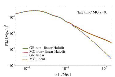
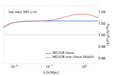
We describe here the effect of applying the standard approach to non linearities to MG theories. This is done using the revised Halofit Takahashi et al. (2012), based on Smith et al. (2003), which is a fitting function of tens of numerical parameters that reproduces the output of a certain set of $\Lambda\mathrm{CDM}$ N-body simulations in a specific range in parameter space as a function of the linear power spectrum. This fitting function is reliable with an accuracy of better than 10% at scales larger than $k\lesssim 1$h/Mpc and redshifts in between $0\leq z\leq 10$ (see Takahashi et al. (2012) for more details). This fitting function can be used within Boltzmann codes to estimate the non-linear contribution which corrects the linear power spectrum as a function of scale and time. We will use the Halofit fitting function as a way of approximating the non-linear power spectrum in our models even though it is really only valid for $\Lambda\mathrm{CDM}$. In Fig. 2, the left panel shows a comparison between the linear and non-linear power spectra calculated by MGCAMB in two different models, our fiducial late-time model (as from Table 1) and GR, both sharing the same $\Lambda\mathrm{CDM}$ parameters. At small length scales (large $k$), the non-linear deviation is clearly visible at scales $k\gtrsim 0.3$ h/Mpc and both MG and GR seem to overlap due to the logarithmic scale used. In the right panel, we can see the ratio between MG and GR for both linear and non-linear power spectra, using the same 5 $\Lambda\mathrm{CDM}$ parameters $\{\Omega_{m},\Omega_{b},h,\,A_{s},n_{s}\}$. We can see clearly that MG in the non-linear regime, using the standard Halofit, shows a distinctive feature at scales in between $0.2\lesssim k\lesssim 2$. This feature however, does not come from higher order perturbations induced by the modified Poisson equations (2, 4), because Halofit, as explained above, is calibrated with simulations within the $\Lambda\mathrm{CDM}$ model and does not contain any information from Modified Gravity. The feature seen here is caused by the different growth rate of perturbations in Modified Gravity, that yields then a different evolution of non-linear structures.

Figure 2: Left: matter power spectra computed with MGCAMB (linear) and MGCAMB+Halofit (non-linear), illustrating the impact of non-linearities at different scales. As an illustrative example, MG in this plot corresponds to the fiducial model in the late-time parametrization defined in Eq. (9). All curves are computed at $z=0$. The green solid line is the GR fiducial in the non-linear case, the blue long-dashed line is also GR but in the linear case. The short-dashed red line is the MG fiducial in the non-linear case and the medium-dashed brown line the MG fiducial in the linear case. Right: in order to have a closer look at small scales, we plot here the ratio of the MG power spectrum to the GR power spectrum for the linear (blue solid) and non-linear (red short-dashed) cases separately. The blue solid line compared to the horizontal grey dashed line, shows the effect of Modified Gravity when taking only linear spectra into account. While the red dashed line, which represents the non-linear case, shows that the ratio to GR presents clearly a bump that peaks around $k\approx 1.0$ h/Mpc, meaning that the power spectrum in MG differs at most 4% from the non-linear power spectrum in GR. We will see later that we are able to discriminate between these two models using future surveys, especially when non-linear scales ($k\gtrsim 0.1$ h/Mpc) are included.

III.2.2 Prescription for mildly non-linear scales including screening

As discussed above, modifications to the $\Phi$ and $\Psi$ potentials make the use of Halofit to compute the evolution at non linear scales unreliable. In order to take into account the non-linear contribution to the power spectrum in Modified Gravity, we investigate here a different method, which starts from the consideration that whenever we modify $\mu$ and $\eta$ with respect to GR, we modify the strength of gravitational attraction in a way universal to all species: this means that, similarly to the case of scalar-tensor or $f(R)$ theories, we need to assume the existence of a non-perturbative screening mechanism, acting at small scales, that guarantees agreement with solar system experiments. In other words, it is reasonable to think that the non-linear power spectrum will have to match GR at sufficiently small scales, while at large scales it is modified. Of course, without having a specific model in mind, it remains arbitrary how the interpolation between the small scale regime and the large scale regime is done. In this paper, we adopt the Hu & Sawicki (HS) Parametrized Post-Friedmann prescription proposed in Hu and Sawicki (2007), which was used for the case of $f(R)$ theories previously by Zhao (2014). Given a MG model, this prescription interpolates between the non-linear power spectrum in Modified Gravity (which is in our case just the linear MG power spectrum corrected with standard Halofit, $P_{\mathrm{HMG}}$) and the non-linear power spectrum in GR calculated with Halofit ($P_{\mathrm{HGR}}$). The resulting power spectrum will be denoted as $P_{\mathrm{nlHS}}$

$$P_{\mathrm{nlHS}}(k,z)=\frac{P_{\mathrm{HMG}}(k,z)+c_{\mathrm{nl}}S_{\mathrm{L}}^{2}(k,z)P_{\mathrm{HGR}}(k,z)}{1+c_{\mathrm{nl}}S_{\mathrm{L}}^{2}(k,z)}\,,$$ (13)

with

$$S_{\mathrm{L}}^{2}(k,z)=\left[\frac{k^{3}}{2\pi^{2}}P_{\mathrm{LMG}}(k,z)\right]^{s}\,.$$ (14)

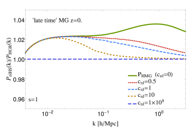
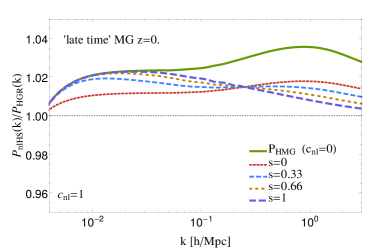
The weighting function $S_{\mathrm{L}}$ used in the interpolation quantifies the onset of non-linear clustering and it is constructed using the linear power spectrum in Modified Gravity ($P_{\mathrm{LMG}}$). The constant $c_{\mathrm{nl}}$ and the constant exponent $s$ are free parameters. In Figure 3 we show the ratio $P_{\mathrm{nlHS}}/P_{\mathrm{HGR}}$, which illustrates the relative difference between the non-linear HS prescription in MG and the Halofit non-linear power spectrum in GR, for different values of $c_{\mathrm{nl}}$ (left panel) and different values of $s$ (right panel). The parameter $c_{\mathrm{nl}}$ controls at which scale there is a transition into a non-linear regime in which standard GR is valid (this can be the case when a screening mechanism is activated); $s$ controls the smoothness of the transition and is in principle a model and redshift dependent quantity. When $c_{\mathrm{nl}}=0$ we recover the Modified Gravity power spectrum with Halofit $P_{\mathrm{HMG}}$; when $c_{\mathrm{nl}}\rightarrow\infty$ we recover the non-linear power spectrum in GR calculated with Halofit $P_{\mathrm{HGR}}$. In Zhao (2014); Zhao et al. (2011); Koyama et al. (2009), the $c_{\mathrm{nl}}$ and $s$ constants were obtained fitting expression (13) to N-Body simulations or to a semi-analytic perturbative approach. In the case of $f(R)$, $s=1/3$ seems to match very well the result from simulations up to a scale of $k=0.5$h/Mpc Koyama et al. (2009). A relatively good agreement up to such small scales is enough for our purposes. In the absence of N-Body simulations or semi-analytic methods available for the models investigated in this work, we will assume unity for both parameters, which is a natural choice, and we will test in Section VI.3 how our results vary for different values of these parameters, namely $c_{\mathrm{nl}}=\{0.1,0.5,\,1,3\}$ and $s=\{0,\,1/3,\,2/3,\,1\}$. This will give a qualitative estimate of the impact of non-linearities on the determination of cosmological parameters.

Figure 3: The ratio of the Modified Gravity non-linear power spectrum using the HS prescription by Hu and Sawicki (2007) ($P_{\mathrm{nlHS}}$) with respect to the GR+Halofit fiducial non-linear power spectrum $P_{\mathrm{HGR}}$, for different values of $c_{\mathrm{nl}}$ (left panel) and $s$ (right panel), illustrated in Eqns.(13, 14). The value $c_{\mathrm{nl}}=0$ (green solid line) corresponds to MG+Halofit $P_{\mathrm{HMG}}$. All curves are calculated at $z=0$. Left: We show the ratio for $c_{\mathrm{nl}}=\{0.5,1.0,10,10^{8}\}$, plotted as short-dashed red, medium-dashed blue, short-dashed brown and medium-dashed purple lines respectively. When $c_{\mathrm{nl}}\rightarrow\infty$, Eqn. (13) corresponds to the limit of $P_{\mathrm{HGR}}$ and therefore the ratio is just 1. The effect of the HS prescription is to grasp some of the features of the non-linear power spectrum at mildly non-linear scales induced by Modified Gravity, taking into account that at very small scales, a screening mechanism might yield again just a purely GR non-linear power spectrum. The parameter $c_{\mathrm{nl}}$ interpolates between these two cases. Right: in this panel we show the effect of the parameter $s$, for $s=\{0,0.33,0.66,1\}$ (short-dashed red, medium-dashed blue, short-dashed brown and long-dashed purple, respectively). Both parameters need to be fitted with simulations in order to yield a reliable match with the shape of the non-linear power spectrum in Modified Gravity, as it was done in Zhao et al. (2011) and references therein. The grey dashed line marks the constant value of 1.

IV Fisher Matrix forecasts

The Fisher matrix formalism (Tegmark et al. (1998); Seo and Eisenstein (2007, 2005)) is one of the most popular tools to forecast the outcome of an experiment, because of its speed and its versatility when the likelihood is approximately Gaussian. Here we apply the Fisher matrix formalism to two different probes, Galaxy Clustering (GC) and Weak Lensing (WL), which are the main cosmological probes for the future Euclid satellite Mukherjee et al. (2008). The background and perturbations quantities we use in the following equations are computed with a version of MGCAMB Zhao et al. (2009); Hojjati et al. (2011) modified in order to account for the binning and the parameterizations described in Section II.

IV.1 Future large scale galaxy redshift surveys

In this work we choose to present results on some of the future galaxy redshift surveys, which are planned to be started and analyzed within the next decade. Our baseline survey will be the Euclid satellite Amendola and others (2013); Laureijs and others (2011). Euclid is a European Space Agency medium-class mission scheduled for launch in 2020. Its main goal is to explore the expansion history of the Universe and the evolution of large scale cosmic structures by measuring shapes and redshifts of galaxies, covering 15000$\text{deg}^{2}$ of the sky, up to redshifts of about $z\sim 2$. It will be able to measure up to 100 million spectroscopic redshifts which can be used for Galaxy Clustering measurements and 2 billion photometric galaxy images, which can be used for Weak Lensing observations (for more details, see Amendola and others (2013); Laureijs and others (2011)). We will use in this work the Euclid Redbook specifications for Galaxy Clustering and Weak Lensing forecasts Laureijs and others (2011), some of which are listed in Tables 2 and 3 and the rest can be found in the above cited references.

Another important future survey will be the Square Kilometer Array (SKA), which is planned to become the world’s largest radiotelescope. It will be built in two phases, phase 1 split into SKA1-SUR in Australia and SKA1-MID in South Africa and SKA2 which will be at least 10 times as sensitive. The first stage is due to finish observations around the year 2023 and the second phase is scheduled for 2030 (for more details, see Yahya et al. (2015); Santos et al. (2015); Raccanelli et al. (2015); Bull et al. (2015)). The first phase SKA1, will be able to measure in an area of 5000$\text{deg}^{2}$ of the sky and a redshift of up to $z\sim 0.8$ an estimated number of about $5\times 10^{6}$ galaxies; SKA2 is expected to cover a much larger fraction of the sky ($\sim$30000$\text{deg}^{2}$), will yield much deeper redshifts (up to $z\sim 2.5$) and is expected to detect about $10^{9}$ galaxies with spectroscopic redshifts Santos et al. (2015). SKA1 and SKA2 will also be capable of performing radio Weak Lensing experiments, which are very promising, since they are expected to be less sensitive to systematic effects in the instruments, related to residual point spread function (PSF) anisotropies Harrison et al. (2016). In this work we will use for our forecasts of SKA1 and SKA2, the specifications computed by Santos et al. (2015) for GC and by Harrison et al. (2016) for WL. The numerical survey parameters are listed in Tables 2 and 3, while the galaxy bias $b(z)$ and the number density of galaxies $n(z)$, can be found in the references mentioned above.

We will also forecast the results from DESI, a stage IV, ground-based dark energy experiment, that will study large scale structure formation in the Universe through baryon acoustic oscillations (BAO) and redshift space distortions (RSD), using redshifts and positions from galaxies and quasars DESI Collaboration et al. (2016a, b); Levi et al. (2013). It is scheduled to start in 2018 and will cover an estimated area in the sky of about 14000$\text{deg}^{2}$. It will measure spectroscopic redshifts for four different classes of objects, luminous red galaxies (LRGs) up to a redshift of $z=1.0$, bright [O II] emission line galaxies (ELGs) up to $z=1.7$, quasars (QSOs) up to $z\sim 3.5$ and at low redshifts ($z\sim 0.2$) magnitude-limited bright galaxies (BLGs). In total, DESI will be able to measure more than 30 million spectroscopic redshifts. In this paper we will use for our forecasts only the specifications for the ELGs, as found in DESI Collaboration et al. (2016a), since this observation provides the largest number density of galaxies in the redshift range of our interest. We cite the geometry and redshift binning specifications in Table 2, while the galaxy number density and bias can be found in DESI Collaboration et al. (2016a).

IV.2 Galaxy Clustering

The distribution of galaxies in space is not perfectly uniform. Instead it follows, up to a bias, the underlying matter power spectrum so that the observed power spectrum $P_{\mathrm{obs}}$ (the Fourier transform of the real-space two point correlation function of the galaxy number counts) is closely linked to the dark matter power spectrum $P(k)$. The observed power spectrum however also contains additional effects like redshift-space distortions due to velocities and a suppression of power due to redshift-uncertainties. Here we follow Seo and Eisenstein (2007), neglecting further relativistic and observational effects, and write the observed power spectrum as

$$P_{\mathrm{obs}}(k,\mu,z)=\frac{D_{A,f}^{2}(z)H(z)}{D_{A}^{2}(z)H_{f}(z)}b^{2}(z)(1+\beta_{d}(z)\mu^{2})^{2}e^{-k^{2}\mu^{2}(\sigma_{r}^{2}+\sigma_{v}^{2})}P(k,z)\,\,\,.$$ (15)

$P_{\mathrm{obs}}(k,\mu,z)$ is the observed power spectrum as a function of the redshift $z$, the wavenumber $k$ and of $\mu\equiv\cos\alpha$, where $\alpha$ is the angle between the line of sight and the 3D-wavevector $\vec{k}$. This observed power spectrum contains all the cosmological information about the background and the matter perturbations as well as corrections due to redshift-space distortions, geometry and observational uncertainties. In the formula, the subscript $f$ denotes the fiducial value of each quantity, $P(k,z)$ is the matter power spectrum, $D_{A}(z)$ is the angular diameter distance, $H(z)$ the Hubble function and $\beta_{d}(z)$ is the redshift space distortion factor, which in linear theory is given by $\beta_{d}(z)=f(z)/b(z)$, with $f(z)\equiv d\ln G/d\ln a$ representing the linear growth rate of matter perturbations and $b(z)$ the galaxy bias as a function of redshift, which we assume to be local and scale-independent. The exponential factor represents the damping of the observed power spectrum, due to two different effects: $\sigma_{z}$ an error induced by spectroscopic redshift measurement errors, which translates into an uncertainty in the position of galaxies at a scale of $\sigma_{r}=\sigma_{z}/H(z)$ and $\sigma_{v}$ which is the dispersion of pairwise peculiar velocities which are present at non-linear scales and also introduces a damping scale in the mapping between real and redshift space. We marginalize over this parameter, similarly to what Bull (2015) and others have done, and we take as fiducial value $\sigma_{v}=300$km/s, compatible with the estimates by de la Torre and Guzzo (2012). We also include the Alcock-Paczynski effect Alcock and Paczynski (1979), by which the $k$ modes and the angle cosine $\mu$ perpendicular and parallel to the line-of-sight get distorted by geometrical factors related to the Hubble function and the angular diameter distance Ballinger et al. (1996); Feldman et al. (1994).

We can then write the Fisher matrix for the galaxy power spectrum in the following form (Seo and Eisenstein, 2007; Amendola et al., 2012):

$$F_{ij}=\frac{V_{\rm survey}}{8\pi^{2}}\int_{-1}^{+1}\mbox{d}\mu\int_{k_{\rm min}}^{k_{\rm max}}\mbox{d}k\,k^{2}\frac{\partial\ln P_{\mathrm{obs}}(k,\mu,z)}{\partial\theta_{i}}\frac{\partial\ln P_{\mathrm{obs}}(k,\mu,z)}{\partial\theta_{j}}\left[\frac{n(z)P_{\mathrm{obs}}(k,\mu,z)}{n(z)P_{\mathrm{obs}}(k,\mu,z)+1}\right]^{2}\,\,.$$ (16)

Here $V_{\rm survey}$ is the volume covered by the survey and contained in a redshift slice $\Delta z$ and $n(z)$ is the galaxy number density as a function of redshift. We will consider the smallest wavenumber $k_{\rm min}$ to be $k_{\rm min}=0.0079\textrm{h/Mpc}$ , while the maximum wavenumber will be $k_{\rm max}=0.15$h/Mpc for the linear forecasts and $k_{\rm max}=0.5$h/Mpc for the non-linear forecasts. In the above formulation of the Galaxy Clustering Fisher matrix, we neglect the correlation among different redshift bins and possible redshift bin uncertainties as was explored recently in Bailoni et al. (2016), we will use for our forecasts the more standard recipe specified in the Euclid Redbook Laureijs and others (2011).

Parameter	Euclid	DESI-ELG	SKA1-SUR	SKA2	Description
$A_{\rm survey}$	15000 $\mbox{deg}^{2}$	14000 $\mbox{deg}^{2}$	5000 $\mbox{deg}^{2}$	30000 $\mbox{deg}^{2}$	Survey area in the sky
$\sigma_{z}$	0.001	0.001	0.0001	0.0001	Spectroscopic redshift error
$\{z_{\rm min},\ z_{\rm max}\}$	{0.65, 2.05}	{0.65, 1.65}	{0.05, 0.85}	{0.15, 2.05}	Min. and max. limits for redshift bins
$\Delta z$	0.1	0.1	0.1	0.1	Redshift bin width

Table 2: Specifications for the spectroscopic galaxy redshift surveys used in this work. The number density of tracers $n(z)$ and the galaxy bias $b(z)$, can be found for SKA in Santos et al. (2015) and for DESI in reference DESI Collaboration et al. (2016a).

IV.3 Weak Lensing

Light propagating through the universe is deflected by variations in the Weyl potential $\Phi+\Psi$, leading to distortions in the images of galaxies. In the regime of small deflections (Weak Lensing) we can write the power spectrum of the shear field as

$$C_{ij}(\ell)=\frac{9}{4}\int_{0}^{\infty}\mbox{d}z\>\frac{W_{i}(z)W_{j}(z)H^{3}(z)\Omega_{m}^{2}(z)}{(1+z)^{4}}\left[\Sigma(\ell/r(z),z)\right]P_{m}(\ell/r(z))\,.$$ (17)

In this expression we used Eqn. (4) to relate the Weyl potential to $\Sigma$ and to the matter power spectrum $P_{m}$ and we use the Limber approximation to write down the conversion $k=\ell/r(z)$, where $r(z)$ is the comoving distance given by

$$r(z)=c\int_{0}^{z}\frac{d\tilde{z}}{H(\tilde{z})}\,.$$ (18)

The indices $i,\>j$ stand for each of the $\mathcal{N}_{bin}$ redshift bins, such that $C_{ij}$ is a matrix of dimensions $\mathcal{N}_{bin}\times\mathcal{N}_{bin}$. The window functions $W_{i}$ are given by

$$W(z)=\int_{z}^{\infty}\mbox{d}\tilde{z}\left(1-\frac{r(z)}{r(\tilde{z})}\right)n(\tilde{z})$$ (19)

where the normalized galaxy distribution function is

$$n(z)\propto z^{2}\exp\left(-(z/z_{0})^{3/2}\right)\,.$$ (20)

Here the median redshift $z_{\rm med}$ and $z_{0}$ are related by $z_{\rm med}=\sqrt{2}z_{0}$. The Weak Lensing Fisher matrix is then given by a sum over all possible correlations at different redshift bins (Tegmark et al., 1998),

$$F_{\alpha\beta}=f_{\rm sky}\sum_{\ell}^{\ell_{\mathrm{max}}}\sum_{i,j,k,l}\frac{(2\ell+1)\Delta\ell}{2}\frac{\partial C_{ij}(\ell)}{\partial\theta_{\alpha}}\textrm{Cov}_{jk}^{-1}\frac{\partial C_{kl}(\ell)}{\partial\theta_{\beta}}\textrm{Cov}_{li}^{-1}\,.$$ (21)

The prefactor $f_{\rm sky}$ is the fraction of the sky covered by the survey. The upper limit of the sum, $\ell_{\mathrm{max}}$, is a high-multipole cutoff due to our ignorance of clustering and baryon physics on small scales, similar to the role of $k_{\rm max}$ in Galaxy Clustering. In this work we choose $\ell_{\mathrm{max}}=1000$ for the linear forecasts and $\ell_{\mathrm{max}}=5000$ for the non-linear forecasts (this cutoff is not necessarily reached at all multipoles $\ell$, as what matters is the minimum scale between $\ell_{\rm max}$ and $k_{\rm max}$, as we discuss below; see also Casas et al. (2015)). In Eqn. (21), $\textrm{Cov}_{ij}$ is the corresponding covariance matrix of the shear power spectrum and it has the following form:

$$\textrm{Cov}_{ij}(\ell)=C_{ij}(\ell)+\delta_{ij}\gamma_{\rm int}^{2}n_{i}^{-1}+K_{ij}(\ell)$$ (22)

where $\gamma_{\rm int}$ is the intrinsic galaxy ellipticity, whose value can be seen in Table 3 for each survey. The shot noise term $n_{i}^{-1}$ is expressed as

$$n_{i}=3600\left(\frac{180}{\pi}\right)^{2}n_{\theta}/\mathcal{N}_{bin}$$ (23)

with $n_{\theta}$ the total number of galaxies per $\text{arcmin}^{2}$ and the index $i$ standing for each redshift bin. Since the redshift bins have been chosen such that each of them contains the same amount of galaxies (equi-populated redshift bins), the shot noise term is equal for each bin. The matrix $K_{ij}(\ell)$ is a diagonal “cutoff” matrix, discussed for the first time in Casas et al. (2015) whose entries increase to very high values at the scale where the power spectrum $P(k)$ has to be cut to avoid the inclusion of uncertain or unresolved non-linear scales. We choose to add this matrix to have further control on the inclusion of non-linearities. Without this matrix, due to the redshift-dependent relation between $k$ and $\ell$, a very high $\ell_{\mathrm{max}}$ would correspond at low redshifts, to a very high $k_{\rm max}$ where we do not longer trust the accuracy of the non-linear power spectrum. Therefore, the sum in Eqn. (21) is limited by the minimum scale imposed either by $\ell_{\mathrm{max}}$ or by $k_{\rm max}$, which is the maximum wavenumber considered in the matter power spectrum $P(k,z)$. As we did for Galaxy Clustering, we use for linear forecasts $k_{\rm max}=0.15$ and for non-linear forecasts $k_{\rm max}=0.5$.

Parameter	Euclid	SKA1	SKA2	Description
$f_{\rm sky}$	0.364	0.121	0.75	Fraction of the sky covered
$\sigma_{z}$	0.05	0.05	0.05	Photometric redshift error
$n_{\theta}$	30	10	2.7	Number of galaxies per arcmin
$\gamma_{\rm int}$	0.22	0.3	0.3	Intrinsic galaxy ellipticity
$z_{0}$	0.9	1.0	1.6	Median redshift over $\sqrt{2}$
$\mathcal{N}_{bin}$	12	12	12	Total number of tomographic redshift bins

Table 3: Specifications for the Weak Lensing surveys Euclid, SKA1 and SKA2 used in this work. Other needed quantities can be found in the references cited in section IV.1. For all WL surveys we use a redshift range between $z=0.5$ and $z=3.0$, using 6 equi-populated redshift bins.

IV.4 Covariance and correlation matrix and the Figure of Merit

The covariance matrix is defined for a d-dimensional vector $p$ of random variables as

$$\mathbf{C}=\langle\Delta p\Delta p^{T}\rangle$$ (24)

with $\Delta p=p-\langle p\rangle$ and the angular brackets $\langle\,\rangle$ representing an expectation value. The matrix $\mathbf{C}$, with all its off-diagonal elements set to zero, is called the variance matrix $V$ and contains the square of the errors $\sigma_{i}$ for each parameter $p_{i}$

$$\mathbf{V}\equiv diag(\sigma_{1}^{2},...,\sigma_{d}^{2})\,\,\,.$$ (25)

The Fisher matrix $\mathbf{F}$ is the inverse of the covariance matrix

$$\mathbf{F}=\mathbf{C}^{-1}\,\,\,.$$ (26)

The correlation matrix $\mathbf{P}$ is obtained from the covariance matrix $\mathbf{C}$, in the following way

$$P_{ij}=\frac{C_{ij}}{\sqrt{C_{ii}C_{jj}}}\,.$$ (27)

If the covariance matrix is non-diagonal, then there are correlations among some elements of $p$. We can observe this also by plotting the marginalized error ellipsoidal contours. The orientation of the ellipses can tell us if two variables $p_{i}$ and $p_{j}$ are correlated ($P_{ij}>0$), corresponding to ellipses with 45 degree orientation to the right of the vertical line or if they are anti-correlated ($P_{ij}<0$), corresponding to ellipses oriented 45 degrees to the left of the vertical line.

To summarize the information contained in the Fisher/covariance matrices we can define a Figure of Merit (FoM). Here we choose the logarithm of the determinant, while another possibility would be the Kullback-Leibler divergence, which is a measure of the information entropy gain, see Appendix E.

The square-root $\sqrt{\det(\mathbf{C})}$ of the determinant of the covariance matrix is proportional to the volume of the error ellipsoid. We can see this if we rotate our coordinate system so that the covariance matrix is diagonal, $\mathbf{C}={\rm diag}(\sigma_{1}^{2},\sigma_{2}^{2},\ldots\sigma_{d}^{2})$, then $\det(\mathbf{C})=\prod_{i}\sigma_{i}^{2}$ and $(1/2)\ln(\det(\mathbf{C}))=\ln\prod_{i}\sigma_{i}$ would indeed represent the logarithm of an error volume. Thus, the smaller the determinant (and therefore also $\ln(\det(\mathbf{C}))$), the smaller is the ellipse and the stronger are the constraints on the parameters. We define

$$\mathrm{FoM}=-\frac{1}{2}\ln(\det(\mathbf{C}))\,,$$ (28)

with a negative sign in front such that stronger constraints lead to a higher Figure of Merit. In the following, the value of the FoM reported in all tables will be obtained including only the dark energy parameters (i.e. the $(\mu_{i},\eta_{i})$ sub-block for the binned case and the $(\mu,\eta)$ sub-block in the smooth functions case), after marginalizing over all other parameters. The FoM allows us to compare not only the constraining power of different probes but also of the different experiments. As the absolute value depends on the details of the setup, we define the relative figure of merit between probe $a$ and probe $b$: $\mathrm{FoM}_{a,b}=-1/2\ln(\det(\mathbf{C_{a}})/\det(\mathbf{C_{b}}))=\mathrm{FoM}_{a}-\mathrm{FoM}_{b}$ and we fix our reference case (probe $b$), for each parametrization, to the Galaxy Clustering observation using linear power spectra with the Euclid survey (labeled as ‘Euclid Redbook GC-lin’ in all figures and tables). The FoM has units of ‘nits’, since we are using the natural logarithm. These are similar to ‘bits’, but ‘nits’ are counted in base $e$ instead of base 2.

An analogous construction allows us to study quantitatively the strength of the correlations encoded by the correlation matrix $\mathbf{P}$. We define the ‘Figure of Correlation’ (FoC) as:

$$\mathrm{FoC}=-\frac{1}{2}\ln(\det(\mathbf{P}))\,.$$ (29)

If the parameters are independent, i.e. fully decorrelated, then $\mathbf{P}$ is just the unit matrix and $\ln(\det(\mathbf{P}))=0$. Off-diagonal correlations will decrease the logarithm of the determinant, therefore making the FoC larger. From a geometrical point of view, the determinant expresses a volume spanned by the vector of (normalized) variables. If these variables are independent, the volume would be maximal and equal to one, while if they are strongly linearly dependent, the volume would be squeezed and in the limit where all variables are effectively the same, the volume would be reduced to zero. Hence, a more positive FoC indicates a stronger correlation of the parameters.

IV.5 CMB Planck priors

Alongside the information brought by LSS probes, we also include CMB priors on the parameterizations considered. In order to obtain these, we analyze the binned and parameterized approaches described in Section II with the Planck+BSH combination of CMB and background (BAO+SN-Ia+$H_{0}$) datasets discussed in the Planck Dark Energy and Modified Gravity paper Planck Collaboration et al. (2016). We use a Markov Chain Monte Carlo (MCMC) approach, using the publicly available code COSMOMC Lewis and Bridle (2002); Lewis (2013), interfaced with our modified version of MGCAMB. The MCMC chains sample the parameter vector $\Theta$ which contains the standard cosmological parameters $\{\omega_{b}\equiv\Omega_{b}h^{2},\,\omega_{c}\equiv\Omega_{c}h^{2},\,\theta_{\rm MC},\,\tau,n_{s},\ln{10^{10}A_{s}}\}$ to which we add the $E_{ij}$ parameters when we parameterize the time evolution of $\mu$ and $\eta$ with continuous functions of the scale factor, and the $\mu_{i},\ \eta_{i}$ parameters in the binned case. On top of these, also the 17 nuisance parameters of the Planck analysis are included. From the MCMC analysis of the Planck likelihood we obtain a covariance matrix in terms of the parameters $\Theta$. We marginalize over the nuisance parameters and over the optical depth $\tau$ since this parameter does not enter into the physics of large scale structure formation.

$\theta$ is usually the ratio of sound horizon to the angular diameter distance at the time of decoupling. Since calculating the decoupling time $z_{\rm CMB}$ is relatively time consuming, as it involves the minimization of the optical transfer function, COSMOMC uses instead an approximate quantity $\theta_{\rm MC}$ based on the following fitting formula from Hu and Sugiyama (1996)

$$z_{\rm CMB} =1048\times(1+0.00124\omega_{b}^{-0.738})$$

$$\times\left(1+0.0783\omega_{b}^{-0.238}/(1+39.5\omega_{b}^{0.763})\right.$$

$$\times\left.(\omega_{d}+\omega_{b})^{0.560/(1+21.1\omega_{b}^{1.81})}\right)$$ (30)

where $\omega_{d}\equiv(\Omega_{c}+\Omega_{\nu})h^{2}$. The sound horizon is defined as

$$r_{s}(z_{\rm CMB})=cH_{0}^{-1}\int_{z_{\rm CMB}}^{\infty}\mbox{d}z\frac{c_{s}}{E(z)}$$ (31)

where the sound speed is $c_{s}=1/\sqrt{3(1+\overline{R}_{b}a)}$with the baryon-radiation ratio being $\overline{R}_{b}a=3\rho_{b}/4\rho_{\gamma}$. $\overline{R}_{b}=31500\Omega_{b}h^{2}(T_{\rm CMB}/2.7\mbox{K})^{-4}$. However, CAMB approximates it as $\overline{R}_{b}a=30000a\Omega_{b}h^{2}$.

Therefore we first marginalize the covariance matrix over the nuisance parameters and the parameter $\tau$, which cannot be constrained by LSS observations. Then, we invert the resulting matrix, to obtain a Planck prior Fisher matrix and then use a Jacobian to convert between the MCMC parameter basis $\Theta_{i}$ and the GC-WL parameter basis $\theta_{i}$. We use the formulas above for the sound horizon $r_{s}$ and the angular diameter distance $d_{A}$ to calculate the derivatives of $\theta_{\rm MC}$ with respect to the parameters of interest. Our Jacobian is then simply (see Appendix A for details)

$$J_{ij}=\frac{\partial\Theta_{i}}{\partial\theta_{j}}\,.$$ (32)

V Results: Euclid forecasts for redshift binned parameters

In this section we analyze the Modified Gravity functions $\mu(a)$ and $\eta(a)$, described in Section II, when they are allowed to vary freely in five redshift bins.

For this purpose, we calculate a Fisher matrix of fifteen parameters: five for the standard $\Lambda\mathrm{CDM}$ parameters $\{\Omega_{m},\Omega_{b},h,\ln 10^{10}A_{s},n_{s}\}$, five for $\mu$ (one for each bin amplitude $\mu_{i}$) and five for $\eta$ (one for each bin amplitude $\eta_{i}$), corresponding to the 5 redshift bins z={0-0.5, 0.5-1.0, 1.0-1.5, 1.5-2.0, 2.0-2.5}. The fiducial values for all fifteen parameters were calculated running a Markov-Chain-Monte-Carlo with Planck likelihood data and can be found in Table 1.

We first show the constraints on our 15 parameters for Galaxy Clustering (GC) forecasts in subsection V.1, while in subsection V.2 we report results for Weak Lensing (WL). In subsection V.3, we comment on the combination of forecasts for GC+WL together with Planck data. All forecasts are performed using Euclid Redbook specifications. Other surveys will be considered for the other two time parameterizations in section VI.1.4 and VI.2.2. For each case, we show the correlation matrix obtained from the covariance matrix and argue that the redshift-binned parameters show a strong correlation, therefore we illustrate the decorrelation procedure for the covariance matrix in subsection V.4 where we also include combined GC+WL and GC+WL+Planck cases.

V.1 Euclid Galaxy Clustering Survey

For the Galaxy Clustering survey, we give results for two cases, one using only linear power spectra up to a maximum wavevector of $k_{\rm max}=0.15$ h/Mpc and another one using non-linear power spectra up to $k_{\rm max}=0.5$ h/Mpc, as obtained by using the HS parameterization of Eqn. (13). For the redshift-binned case, we will report forecasts only for a Euclid survey, using Euclid Redbook specifications which are detailed in section IV.2.

Figure 4: Correlation matrix $\mathbf{P}$ defined in (27) obtained from the covariance matrix in the MG-binning case, for a Galaxy Clustering Fisher forecast using Euclid Redbook specifications. Left panel: Linear forecasts. Here there are strong positive correlations among the $\mu_{i}$ and $\eta_{i}$ parameters and anti-correlations between $\ln 10^{10}A_{s}$ and the $\mu_{i}$ parameters, as well as between $\mu_{i}$ and $\eta_{i}$. The FoC in this case is $\approx 65$. (see Eqn. (29) for its definition). Right panel: Non-linear forecasts using the HS prescription. Interestingly, the anti-correlations between $\ln 10^{10}A_{s}$ and $\mu_{i}$ have disappeared, as well as the correlations among the $\mu_{i}$ parameters. The FoC is in this case $\approx 32$, meaning that the variables are much less correlated than in the linear case. This is due to the fact that taking into account non-linear structure formation breaks degeneracies between the primordial amplitude parameter and the modifications to the Poisson equation.

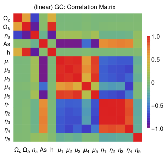
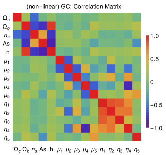
We calculate the Fisher matrix for the 15 parameters $\theta=\{\Omega_{m},\Omega_{b},h,\ln 10^{10}A_{s},n_{s},\mu_{i},\eta_{i}\}$ where $\eta_{i}$ and $\mu_{i}$ represent ten independent parameters, one for each function at each of the 5 redshift bins corresponding to the redshifts z={0-0.5, 0.5-1.0, 1.0-1.5, 1.5-2.0, 2.0-2.5}. As a standard procedure, we marginalize over the unknown bias parameters. From the covariance matrix, defined previously in Eqn. (24), we obtain the correlation matrix $P_{ij}$ defined in Eqn. (27) for the set of parameters $\theta_{i}$. In Figure 4 we show the matrix $P_{ij}$ in the linear (left panel) and non-linear-HS (right panel) cases. Redder (bluer) colors signal stronger correlations (anti-correlations).

A covariance matrix that contains strong correlations among parameter A and B, means that the experimental or observational setting has difficulties distinguishing between A and B for the assumed theoretical model, i.e. this represents a parameter degeneracy. Therefore if for example parameter A is poorly constrained, then parameter B will be badly constrained as well. The appearance of correlations among parameters is linked to the non-diagonal elements of the covariance matrix. Subsequently, this means that the fully marginalized errors on a single parameter, will be larger if there are strong correlations and will be smaller (closer to the value of the fully maximized errors) if the correlations are negligible.

In the linear case, $\mu_{i}$ and $\eta_{i}$ parameters show correlations among each other, while the primordial amplitude parameter $\ln 10^{10}A_{s}$ exhibits a strong anti-correlation with all the $\mu_{i}$. This can be explained considering that a larger growth of structures in linear theory can also be mimicked with a larger initial amplitude of density fluctuations.

Interestingly, including non-linear scales in the analysis (right panel of Fig. 4) leads to a strong suppression of the correlations among the $\mu_{i}$. Also the correlation between these and $\ln 10^{10}A_{s}$ is suppressed as a change in the initial amplitude of the power spectrum is not able to compensate for a modified Poisson equation when non-linear evolution is considered.

As discussed in Section IV.4, we can also express the difference between the correlation matrix of the linear forecast and the non-linear forecast in a more quantitative way, by computing the determinant of the correlation matrix, or equivalently the FoC (29). If the correlations were negligible, this determinant would be equal to one (and therefore its FoC would be 0), while if the correlations were strong, the determinant would be closer to zero with a corresponding large positive value of the FoC. For the linear forecast, the FoC is about $62$, while for the non-linear forecast, it is much smaller at approximately $35$. In Table V.1 we show the 1$\sigma$ constraints obtained on $\ln{(10^{10}A_{s})}$ and on the $\mu_{i}$ and $\eta_{i}$ parameters, both in the linear and non-linear cases for a Euclid Redbook GC survey (top rows). While linear GC alone ($k_{\rm max}$ = 0.15 h/Mpc) is not very constraining in any bin, the inclusion of non-linear scales ($k_{\rm max}$= 0.5 h/Mpc) drastically reduces errors on the $\mu_{i}$ parameters: the first three bins in $\mu_{i}$ (0. < z < 1.5 ) are the best constrained, to less than $10\%$, with the corresponding $\eta_{i}$ constrained at 20$\%$ by non-linear GC alone. This is also visible in the FoM which increases by 19 nits (‘natural units’, similar to bits but using base $e$ instead of base 2), nearly 4 nits per redshift bin on average, when including the non-linear scales. The fact that the error on $\ln 10^{10}A_{s}$ improves from 90% to 0.68% shows that the decorrelation induced by the non-linearities breaks the degeneracy with the amplitude and therefore improves considerably the determination of cosmological parameters. This shows that it is important to include non-linear scales in GC surveys (and not only in Weak Lensing ones, which is usually more expected and will be shown in the next subsection).

Euclid (Redbook)	$\ell\mathcal{A}_{s}$	$\mu_{1}$	$\mu_{2}$	$\mu_{3}$	$\mu_{4}$	$\mu_{5}$	$\eta_{1}$	$\eta_{2}$	$\eta_{3}$	$\eta_{4}$	$\eta_{5}$	MG FoM
Fiducial	3.057	1.108	1.027	0.973	0.952	0.962	1.135	1.160	1.219	1.226	1.164	relative
GC (lin)	160%	119%	159%	183%	450%	1470%	509%	570%	586%	728%

& 0 GC (nl-HS) 0.8% 7.0% 6.7% 10.9% 27.4% 41.1% 20% 24.3% 19.9% 38.2% 930% 19 WL (lin) 640% 165% 2210% 4150% 13100% 22500% 2840% 3140% 8020% 29300% 39000% -27 WL (nl-HS) 7.3% 188% 255% 419% 222% 206% 330% 488% 775% 8300% 9380% -10 GC+WL (lin) 11.3% 5.8% 10% 19.2% 282% 469% 7.9% 9.6% 16.1% 276% 2520% 12 GC+WL+Planck (lin) 1.1% 3.4% 4.8% 7.8% 9.3% 13.1% 6.2% 7.7% 9.1% 12.7% 23.6% 27 GC+WL (nl-HS) 0.8% 2.2% 3.3% 8.2% 24.8% 34.1% 3.6% 5.1% 8.1% 25.4% 812% 24 GC+WL+Planck (nl-HS) 0.3% 1.8% 2.5% 5.8% 7.8% 10.3% 3.2% 4.1% 5.9% 9.6% 19.5% 33 GC+WL+Planck (nl-Halofit) 0.4% 2.0% 2.4% 5.1% 7.4% 10.2% 3.5% 4.1% 5.8% 9.2% 18.9% 33

Table 4: 1$\sigma$ fully marginalized errors (as a percentage of the corresponding fiducial) on cosmological parameters for Euclid (Redbook) Galaxy Clustering and Weak Lensing surveys, alone and combining the two probes. We compare forecasts using linear spectra (lin) and forecasts using the nonlinear HS prescription (nl-HS). In Galaxy Clustering, the cutoff is set to $k_{\rm max}=0.15$ h/Mpc in the linear case and $k_{\rm max}=0.5$ h/Mpc in the non-linear case. For WL, the maximum cutoff in the linear case is at $\ell_{\rm max}=1000$, while in the nl-HS case it is $\ell_{\rm max}=5000$. At the bottom, we add on top a Planck prior (see section IV.5). For comparison, we also show in the last row the combined GC+WL+Planck, using just Halofit power spectra. The last column indicates the relative Figure of Merit ($\text{FoM}_{a,b}$) of the MG parameters in nits (‘natural units’, i.e. using the natural logarithm), with respect to our reference GC linear case, see (28) and surrounding text. A larger FoM indicates a more constraining probe. We notice a considerable improvement, in both GC and WL, when non-linearities are included. The combination GC+WL in the linear case constrains the MG parameters in the first two bins (z < 1.0 ) to less than 10$\%$ and including Planck priors allows to access higher redshifts with the same accuracy. A significant improvement in the constraints is obtained when adding the non-linear regime, in agreement with the observed reduction in correlation seen in Figs. 4 and 5. This is especially well exemplified by the error on $\ell\mathcal{A}_{s}\equiv\ln(10^{10}A_{s})$, which reduces from 160% to 0.82%, from the linear to the non-linear forecast in the GC case and from 640% to 7.3% in the WL case. Finally, we note that since we are showing errors on $\mu$ and $\eta$, WL seems to be unfairly poor at constraining parameters. However, when converting this errors into errors on $\Sigma$, which is directly measured by WL, the constrains on $\Sigma_{1,2,3}$ are slightly better, of the order of 40% for WL(nl-HS) as can be guess from the degeneracy directions shown in Fig. 14. The FoM itself is nearly unaffected by the choice of $\{\mu,\eta\}$ vs $\{\mu,\Sigma\}$ as it is rotationally invariant.

V.2 Euclid Weak Lensing Survey

In the case of Weak Lensing, the linear forecast is performed with linear power spectra up to a maximum multipole $\ell_{\rm max}=1000$, while the non-linear forecast is performed with non-linear spectra up to a maximum multipole of $\ell_{\rm max}=5000$, as explained in section IV. Since we limit our power spectrum to a maximum in $k$-space, as explained in section IV.3, these multipole values are not reached at every redshift. Like for GC, also for WL it is very important to include information from the non-linear power spectrum, since in that range will lie most of the constraining power of next-generation surveys like Euclid. In Figure 5 we show the correlation matrices for the linear (left panel) and non-linear (right panel) Fisher Matrix forecasts. In this case, as opposed to the GC correlation matrices, it is not visually clear which case is more correlated than the other. At a closer look, in the linear case we can observe strong anti-correlations between the $\mu_{j}$ and $\eta_{j}$ parameters for $j={2,3,4,5}$ and an anti-correlation between $\eta_{1}$ and the primordial amplitude $\ln 10^{10}A_{s}$. In the non-linear case, the primordial amplitude parameter is effectively decorrelated from the Modified Gravity parameters, and the anti correlation between $\mu_{j}$ and the $\eta_{j}$ affects the first three bins (effectively increasing degeneracies in the first bin). The anti-correlation between these two sets of parameters is expected, since WL is sensitive to $\Sigma$, which is a product of $\eta$ and $\mu$, c.f. Eqn. (5). The decrease of correlation when going from the linear to the non-linear case is confirmed, also quantitatively, by the FoC: the one for the linear case is of $\approx 69$, larger than the one for the non-linear case $\approx 32$. Once again, the inclusion of non-linear scales breaks degeneracies, especially among the linear amplitude of the power spectrum and the MG parameters.

Figure 5: Correlation matrix obtained from the covariance matrix in the MG-binning case, for a Weak Lensing Fisher Matrix forecast using Euclid Redbook specifications. Left panel: linear forecasts. Strong anti-correlations are present between the $\mu_{i}$ and the $\eta_{i}$ parameters for the same value of i in 2,3,4,5. The amplitude $\ln(10^{10}A_{s})$ parameter is mostly uncorrelated except with $\eta_{1}$. The FoC (29) in this case is approximately $69$. Right panel: non-linear forecasts using the HS prescription. Here the same trend as in the linear case is present, with just subtle changes. The FoC in this case is about $32$, meaning that the variables are indeed less correlated than in the linear case. The parameter $\ln(10^{10}A_{s})$ is effectively not correlated to other parameters, and the anti-correlation of $\mu_{i}$ and the $\eta_{i}$ for the same value of the index i is present in the first three bins. The anti-correlation between these two sets of parameters is expected, since WL is sensitive to the Weyl potential $\Sigma$, which is a product of $\mu$ and $\eta$.

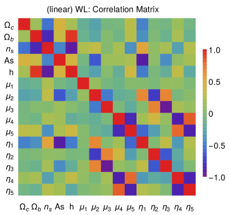
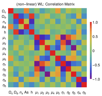
Table V.1 shows the corresponding 1$\sigma$ marginalized errors on $\ln{(10^{10}A_{s})}$ and on the $\mu_{i}$ and $\eta_{i}$, both in the linear and non-linear cases for a Euclid Redbook WL survey. As in the case of GC, linear WL cannot constrain alone any of the amplitudes of the Modified Gravity parameters $\mu_{i}$ and $\eta_{i}$ for any redshift bin. Being able to include non-linear scales improves constraints on the amplitude $\ln(10^{10}A_{s})$ by a factor 100. The 1$\sigma$ errors on $\mu_{i}$ and $\eta_{i}$ improve up to one order of magnitude, with the FoM increasing by 17 nits, although remaining quite unconstraining for Modified Gravity parameters in all redshift bins. Notice, however, that the 1$\sigma$ error on $\mu_{1}$ from WL in the linear case is slightly smaller than in the non-linear case. This can be attributed to the fact that in the linear case, $\mu_{1}$ is uncorrelated to any other parameter, as shown in Figure 5 and on that specific bin (0 < z < 0.5) non-linearities don’t seem to improve the constraints on this parameter.

V.3 Combining Euclid Galaxy Clustering and Weak Lensing, with Planck data

The combination of Galaxy Clustering and Weak Lensing is expected to be very powerful for Modified Gravity parameters as they measure two different combinations of $\mu$ and $\eta$, thus breaking their degeneracy as illustrated in Fig. 14. This is shown in Table V.1, where the sensitivity drastically increases with respect to the two separate probes, especially in the low redshifts bins $(0.<z<1.5)$, where the lensing signal is dominant. Adding non-linearities further doubles the FoM. The Planck data constrains mostly the standard $\Lambda\mathrm{CDM}$ parameters and has only a limited ability to constrain the MG sector. However, the additional information breaks parameter degeneracies and in this way significantly decreases the uncertainties on all parameters, so that the linear GC+WL+Planck is comparable to the non-linear GC+WL. Also, quantitatively, the correlation among parameters is reduced by combining GC+WL with Planck data. The FoC in this case is of $\approx 22$. We also see in Table V.1 that the differences between the non-linear prescription adopted here (nl-HS) and a straightforward application of Halofit to the MG case (nl-Halofit) is not very large. We will investigate further the impact of the parameters used in the non-linear prescription in section VI.3.

V.4 Decorrelation of covariance matrices and the Zero-phase Component Analysis

In the previous subsections we highlighted how the MG parameters and the amplitude of the primordial power spectrum exhibit significant correlations and showed how including non-linearities helps to decorrelate them. Even without including non-linearities, however, it is interesting to investigate how we can completely decorrelate the parameters, identifying in this way those parameter combinations which are best constrained by data.

Given again a d-dimensional vector $p$ of random variables (our originally correlated parameters), we can calculate its covariance matrix $\mathbf{C}$ defined in Eqn. (24). The process of decorrelation is the process of making the matrix $\mathbf{C}$ a diagonal matrix.

Let us define some important identities. The covariance matrix can be decomposed in its eigenvalues (the elements of a diagonal matrix $\Lambda$) and eigenvectors (the rows of an orthogonal matrix $U$).

$$\mathbf{C}=U\Lambda U^{T}\quad\Leftrightarrow\quad\mathbf{F}=U\Lambda^{-1}U^{T}\,\,\,,$$ (33)

where $\mathbf{F}$ is the Fisher Matrix.

It is possible to show that applying a transformation matrix $W$ to the $p$ parameter vector, thus obtaining a new vector of variables $q=Wp$, the covariance matrix of the transformed vector $q$ is whitened (i.e. it is the identity matrix, and whitening is defined as the process of converting the covariance matrix into an identity matrix)

$$\mathbf{\tilde{C}} =W\langle\Delta\hat{p}\Delta\hat{p}^{T}\rangle W^{T}=\langle\Delta\hat{q}\Delta\hat{q}^{T}\rangle$$ (34)

$$=\mathbb{1}\,\,\,.$$

This means that the transformed $q$ parameters are decorrelated, since their correlation matrix is diagonal. The choice of $W$ is not unique as several possibilities exist; we focus on a particular choice in the rest of the paper referred to as Zero-phase Component Analysis (ZCA, first introduced by Bell and Sejnowski (1997) in the context of image processing), but we show two other possible choices and their effect on the analysis in Appendix C.

Zero-phase Component Analysis (sometimes also called Mahalanobis transformation Kessy et al. (2015)) is a specific choice of decorrelation method that minimizes the squared norm of the difference between the $q_{i}$ and the $p_{i}$ vector $\|\vec{p}-\vec{q}\|$, under the constraint that the vector $\vec{q}$ should be uncorrelated Kessy et al. (2015). In this way the uncorrelated variables $q$ will be as close as possible to the original variables $p$ in a least squares sense. This is achieved by using the $W$ matrix:

$$W\equiv F^{1/2}\,\,\,.$$ (35)

Then in this case, the covariance matrix is whitened, by following Eqn. (34):

$$\tilde{C}=F^{1/2}F^{-1}F^{1/2}=\mathbb{1}\,\,\,.$$ (36)

In our case, since we do not want to whiten, but just decorrelate the covariance matrix, we renormalize the $W$ matrix by multiplying with a diagonal matrix $N_{jj}\equiv\sum_{j}(W_{ij}^{-2})$, such that the sum of the square of the elements on each row of the new weighting matrix $\tilde{W}\equiv NW$, is equal to unity; therefore the final transformed covariance is still diagonal but is not the identity matrix:

$$\tilde{C}=\tilde{W}C\tilde{W}=N^{2}\mathbb{1}$$ (37)

and at the same time we ensure that the vector of new variables $q_{i}$ will have the same norm as the old vector of variables $p_{i}$.

V.4.1 ZCA for Galaxy Clustering

From Fig. 4 we can see that the correlations are present in sub-blocks, one for the standard $\Lambda\mathrm{CDM}$ parameters and another one for the Modified Gravity parameters. The exception lies in the linear case where $\ell\mathcal{A}_{s}\equiv\ln{(10^{10}A_{s})}$ is strongly anti-correlated with all the $\mu_{i}$ and positively correlated with the $\eta_{i}$. To use a more objective criterion, we choose the $10\times 10$ block of MG parameters $\mu_{i}$ and $\eta_{i}$ with parameter indices 6 to 15, and only add to this block a $\Lambda\mathrm{CDM}$ parameter with index $a$ if the following condition is satisfied:

$$\sum_{i=6}^{i=15}(P_{ai})^{2}\geq 1$$

where the index $a$ corresponds to one of the first five standard parameters. For Galaxy Clustering, the only index satisfying this condition is $a=4$ in the linear case, corresponding to $\ell\mathcal{A}_{s}\equiv\ln{(10^{10}A_{s})}$: i.e. the standard parameter corresponding to the amplitude is, as said, degenerate with Modified Gravity parameters $\mu_{i}$ and $\eta_{i}$. In the non-linear case no parameter satisfies this condition (because, as we have seen, non-linearities are able to eliminate correlation with the amplitude), but for consistency we will use the same vector of 11 parameters $p_{i}=\left\{\ell\mathcal{A}_{s},\mu_{i},\eta_{i}\right\}$ for our decorrelation procedure. Therefore we will also have 11 transformed uncorrelated $q_{i}$ parameters, function of the original $p_{i}$ parameters, in all the cases presented below.

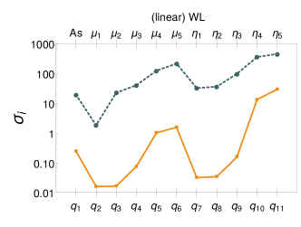
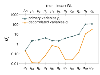
Figure 6 shows the coefficients that relate the $q_{i}$ parameters to the original $p_{i}$ ones, in the linear (left panel) and the non-linear (right panel) cases, also shown explicitly in Tables 11 and 12 of Appendix D. We plot in Figure 7 a comparison between the 1$\sigma$ errors on the primary parameters $p_{i}$ (represented by circles connected with dark green dashed lines) and the decorrelated parameters $q_{i}$ (represented by squares connected with orange solid lines). In the linear case (left panel), we can see that the errors on the $q_{i}$ parameters are 2 orders of magnitude better than the errors on the $p_{i}$ parameters. In the non-linear case (right panel) the improvement is of at most 1 order of magnitude and that for a completely decorrelated parameter like $\ell\mathcal{A}_{s}$, the error on its corresponding $q_{i}$ is exactly the same. This shows that a decorrelation procedure is still worth to do, even when including the non-linear regime, even if the degeneracy with the amplitude is already completely broken thanks to the non-linear prescription. The fact that the curve of 1$\sigma$ errors for the $q_{i}$ follows the same pattern as the curve for the $p_{i}$ errors, is due to the fact that we have used a ZCA decomposition (see Section V.4) and therefore the $q_{i}$ are as similar as possible to the $p_{i}$.

Figure 6: Entries of the matrix $W$ that relates the $q_{i}$ parameters to the original $p_{i}$ ones, after applying the ZCA decorrelation of the covariance matrix in the linear and non-linear GC cases. This matrix shows for each new variable $q_{i}$ on the vertical axis, the coefficients of the linear combination of parameters $\mu_{i}$, $\eta_{i}$ and $A_{s}$ that give rise to that variable $q_{i}$. The red (blue) colors, indicate a large (small) contribution of the respective variable on the horizontal axis. Left panel: linear forecast for Euclid Redbook specifications. Right panel: non-linear forecast for Euclid Redbook specifications, using the HS prescription. In both cases one can observe that most $q_{i}$ parameters have only small or negligible contributions from $\mu_{5}$ and $\eta_{5}$, which are found to be the less constrained bins.

Figure 7: Results for a Euclid Redbook GC survey, with redshift-binned parameters, before and after applying the ZCA decorrelation. Each panel shows the 1$\sigma$ fully marginalized errors on the primary parameters $p_{i}$ (green dashed lines), and the 1$\sigma$ errors on the decorrelated parameters $q_{i}$ (orange solid lines). Left: linear forecasts, performed using linear power spectra up to a maximum wavenumber $k_{\rm max}=0.15$h/Mpc. Right: non-linear forecasts using non-linear spectra with the HS prescription up to a maximum wavenumber $k_{\rm max}=0.5$h/Mpc. In the linear case, the errors on the decorrelated $q_{i}$ parameters are about 2 orders of magnitude smaller than for the primary parameters, while in the non-linear HS case, the improvement in the errors is of one order of magnitude. This means that applying a decorrelation procedure is worth even when non-linearities are considered. In both cases for GC, the least constrained parameters are $\mu_{5}$ and $\eta_{5}$, corresponding to $2.0<z<2.5$.

Figure 8: Best constrained modes for a Euclid Redbook GC survey, with $\mu$ and $\eta$ binned in redshift, after transforming into uncorrelated $q$ parameters via ZCA. Each of the four best constrained parameters $q_{i}$, shown in the panels, is a linear combination of the primary parameters $p_{i}$. The $q_{i}$ in the legends are ordered from left to right, from the best constrained to the least constrained.

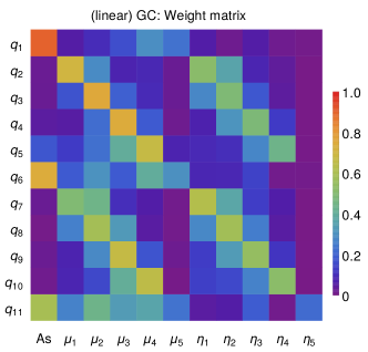
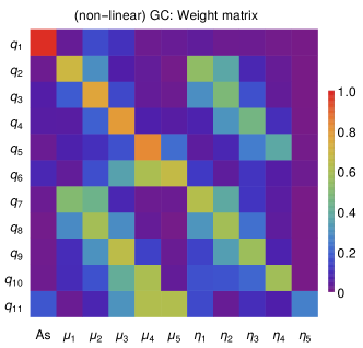
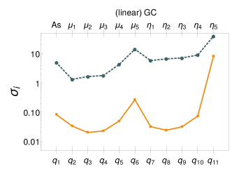
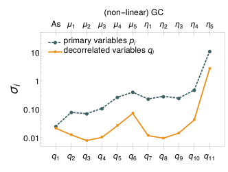
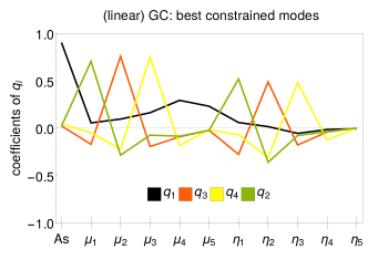
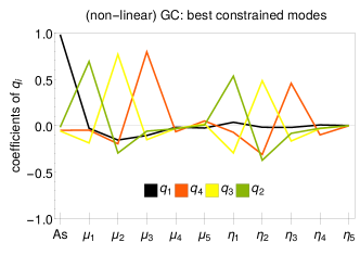
We are interested in finding the best combination of primary parameters $p_{i}$ giving rise to the best constrained uncorrelated parameters $q_{i}$. In order to find the errors on the parameters $q_{i}$, we need to look at the diagonal of the decorrelated covariance matrix $\mathbf{\tilde{C}}$ expressed in Eqn. (37) and identify the $q_{i}$ parameters with the smallest relative errors ($\sigma_{q_{i}}/q_{i}$): we find than in the linear GC case, the best constrained combinations of primary parameters (ordered from most to least constrained) are given approximately by:

$$q_{1} =+0.9\ell\mathcal{A}_{s}+0.32\mu_{4}$$ (38)

$$q_{3} =+0.75\mu_{2}-0.29\eta_{1}+0.50\eta_{2}$$

$$q_{4} =-0.25\mu_{2}+0.74\mu_{3}-0.32\eta_{2}+0.49\eta_{3}$$

$$q_{2} =+0.70\mu_{1}-0.30\mu_{2}+0.52\eta_{1}-0.36\eta_{2}\,\,\,.$$

In contrast, for the non-linear GC case, the parameter $\ell\mathcal{A}_{s}\equiv\ln{(10^{10}A_{s})}$ is not correlated to any other, and therefore it is well constrained on its own. The best 4 constrained parameters (ordered from most to least constrained) in the non-linear case, are:

$$q_{1} =+0.99\ell\mathcal{A}_{s}$$ (39)

$$q_{4} =-0.28\mu_{2}+0.76\mu_{3}-0.33\eta_{2}+0.47\eta_{3}$$

$$q_{3} =+0.73\mu_{2}-0.32\eta_{1}+0.49\eta_{2}$$

$$q_{2} =+0.68\mu_{1}-0.35\mu_{2}+0.52\eta_{1}-0.37\eta_{2}\,\,\,.$$

The best constrained decorrelated parameters $q_{i}$ for a Euclid GC survey, expressed in the set of Equations (38) (linear) and (39) (non-linear HS), can be seen graphically in Fig. 8 for the linear (left panel) and non-linear HS (right panel) cases respectively. From these combinations we see that a survey like Euclid, using GC only, will be sensitive to Modified Gravity parameters $\mu$ and $\eta$ mainly in the first three redshift bins, corresponding to a range $0.<z<1.5$. The complete matrix $W$ of coefficients relating the $q_{i}$ to the $p_{i}$ parameters, can be found in Tables 11 and 12 of Appendix D.

V.4.2 ZCA for Weak Lensing

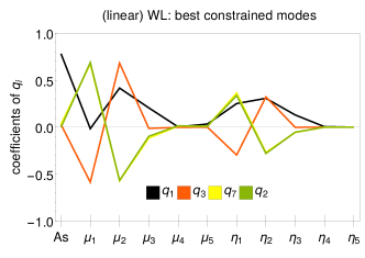
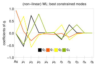
We apply the same decorrelation procedure to the WL case, obtaining the $q$ vectors shown in the weight matrix of Figure 9 again reported explicitly in Tables 13 and 14 in Appendix D.

Figure 9: Entries of the matrix $W$ that relates the $q_{i}$ parameters to the original $p_{i}$ ones, after applying the ZCA decorrelation of the covariance matrix in the linear and non-linear WL cases. This matrix shows for each new variable $q_{i}$ on the vertical axis, the coefficients of the linear combination of parameters $\mu_{i}$, $\eta_{i}$ and $A_{s}$ that give rise to that variable $q_{i}$. The red (blue) colors, indicate a large (small) contribution of the respective variable on the horizontal axis. Left panel: linear forecast for Weak Lensing Euclid Redbook specifications. Right panel: non-linear forecast for Weak Lensing Euclid Redbook specifications, using the HS prescription. As for GC, most $q_{i}$ parameters have only small or negligible contributions from $\mu_{5}$ and $\eta_{5}$, which are found to be the less constrained bins.

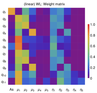
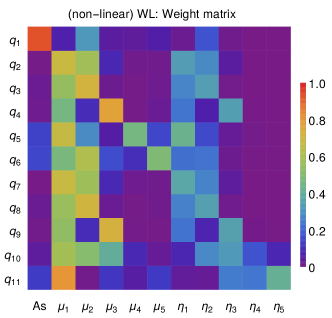
In Figure 10 we show the comparison between the errors on the primary parameters $p_{i}$ and the de-correlated ones $q_{i}$. As for the GC case, the errors in the linear case improve by 2 orders of magnitude after applying the decorrelation procedure (left panel). In the non-linear case (right panel) the improvement is smaller, but still worth to do, especially to constrain $q_{2},q_{3},q_{7},q_{8}$.

Figure 10: Results for a Euclid Redbook WL survey, with redshift-binned parameters, before and after applying the ZCA decorrelation. Each panel shows the 1$\sigma$ fully marginalized errors on the primary parameters $p_{i}$ (green dashed lines), and the 1$\sigma$ errors on the decorrelated parameters $q_{i}$ (orange solid lines). Left: Linear forecasts, performed with an $\ell_{\rm max}=1000$ and linear matter power spectra. Right: Non-linear forecasts using the non-linear spectra with the HS prescription, up to an $\ell_{\rm max}=5000$. The errors in the non-linear HS case, are about 1 order of magnitude smaller than in the linear case. For the best constrained $q_{i}$ parameters, the decorrelated errors are up to 2 orders of magnitude smaller than the corresponding fully marginalized parameters on the parameters $p_{i}$.

More generally, as we did for the GC case in the previous section, we look for the $q_{i}$ parameters with the smallest relative errors ($\sigma_{q_{i}}/q_{i}$) and find in the linear WL case, that the best constrained combinations (ordered from most to least constrained) of primary parameters are given approximately by:

$$q_{1} =+0.76\ell\mathcal{A}_{s}+0.48\mu_{2}+0.33\eta_{2}$$ (40)

$$q_{3} =-0.59\mu_{1}+0.67\mu_{2}-0.30\eta_{1}+0.32\eta_{2}$$

$$q_{7} =+0.65\mu_{1}-0.60\mu_{2}+0.36\eta_{1}-0.28\eta_{2}$$

$$q_{2} =+0.67\mu_{1}-0.59\mu_{2}+0.33\eta_{1}-0.29\eta_{2}\,\,\,.$$

This means that WL in the linear case will only be able to constrain combinations of the first two redshift bins in $\mu$ and $\eta$ (corresponding to $0.<z<1.0$). This can also be observed graphically in the left panel of Figure 11. For the non-linear WL case, the combinations remain practically the same, except for $q_{1}$, which will depend much more strongly on the parameter $\ell\mathcal{A}_{s}$. The best 4 constrained parameters in this case, are (ordered from most to least constrained):

$$q_{3} =-0.55\mu_{1}+0.71\mu_{2}+-0.27\eta_{1}+0.34\eta_{2}$$ (41)

$$q_{1} =+0.93\ell\mathcal{A}_{s}-0.32\mu_{2}$$

$$q_{2} =+0.67\mu_{1}-0.60\mu_{2}+0.33\eta_{1}-0.29\eta_{2}$$

$$q_{4} =-0.46\mu_{1}+0.29\mu_{2}+0.73\mu_{3}+0.31\eta_{3}\,\,\,.$$

These combinations can also be visualized in the right panel of Figure 11. The complete matrix $W$ of coefficients relating the $q_{i}$ to the $p_{i}$ parameters, can be found in Tables 11 and 12 of Appendix D.

Figure 11: Best constrained modes for a Euclid Redbook WL survey, with $\mu$ and $\eta$ binned in redshift, after transforming into uncorrelated $q$ parameters via ZCA. Each of the four best constrained parameters $q_{i}$, shown in the panels, is a linear combination of the primary parameters $p_{i}$. $q_{i}$ in the label are ordered from the best constrained to the least constrained.

V.4.3 ZCA for Weak Lensing + Galaxy Clustering + CMB Planck priors

As mentioned earlier, Galaxy Clustering and Weak Lensing are particularly important, combined together, to constrain Modified Gravity parameters, as they probe two independent combinations of the gravitational potentials. We now show results for their combination, using for both the non-linear HS prescription, together with a Planck prior (which was obtained by performing an MCMC analysis on Planck+BSH background data, as specified in Section IV.5). Notice that we neglect here any information coming from the cross correlation of the two probes; we therefore assume that these two observables are independent of each other and we simply add the GC and WL Fisher matrices to obtain our combined results; this appears to be a conservative (pessimistic) choice Lacasa and Rosenfeld (2016). In Table V.1, we can see that the inclusion of the Planck prior improves considerably certain parameters, especially the less constrained ones by GC+WL, namely $\mu_{4,5}$ and $\eta_{4,5}$. In terms of correlations, we can observe in the left panel of Fig. 12, that the structure of the correlation matrix resembles the one of the linear WL case (Fig. 5), except that the block of standard $\Lambda\mathrm{CDM}$ parameters is much less correlated and that the anti-correlation among $\mu_{i}$ and $\eta_{i}$ is much stronger now. On the other hand, applying the decorrelation procedure (Section V.4), the weight matrix $W$ (right panel of Fig. 12), resembles the $W$ matrix observed in the non-linear GC case, illustrated in Figure 6). Notice that now the variables $q_{i}$ depend quite strongly on only one of the $\mu_{i}$ for $i=\{1,2,3,4\}$, while the $q_{i}$ for $i=\{6,7,8,9,10\}$ depend on a balanced sum of $\mu_{i}$ and $\eta_{i}$ for $i=\{6,7,8,9,10\}$.

Figure 12: Results for the combined forecasts of Euclid Redbook GC+WL using the non-linear HS prescription together with the addition of Planck CMB priors. Left panel: correlation matrix obtained from the covariance matrix in the MG-binning case. Red (purple blue) colors represent strong positive (negative) correlations. The structure of this matrix is considerably diagonal, except for the strong anti-correlations of the pair $(\mu_{i},\eta_{i})$ for $i=\{1,2,3,4,5\}$, which resembles the correlations found for the WL case alone (see Figure 5). However, the sub-block of standard cosmological parameters is now much more diagonal and shows less correlations than in the GC (Fig. 4) or WL cases. The natural FoC (defined in 29) in this case is $\approx 22$, showing that the variables are much less correlated than in the two previous cases. Right panel: entries of the matrix $W$ for the ZCA decorrelation of the covariance matrix. This matrix shows for each new variable $q_{i}$ on the vertical axis, the coefficients of the linear combination of parameters $\mu_{i}$ and $\eta_{i}$ that give rise to that variable $q_{i}$. The red (blue) colors, indicate a large (small) contribution of the respective variable on the horizontal axis.

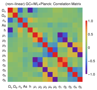
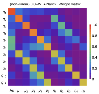
Finally, in this combined case the best constrained $q_{i}$ variables, are $q_{1},\;q_{2},\;q_{3},\;$, $q_{4}$ approximately given by:

$$q_{1} =+0.93\ell\mathcal{A}_{s}$$ (42)

$$q_{2} =+0.84\mu_{1}+0.48\eta_{1}$$

$$q_{3} =+0.80\mu_{2}-0.26\eta_{1}+0.45\eta_{2}$$

$$q_{4} =+0.28\ell\mathcal{A}_{s}+0.79\mu_{3}-0.29\eta_{2}+0.39\eta_{3}\,\,\,.$$

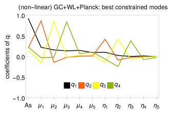
These combinations of primary parameters are illustrated in the right panel of Figure 13. The combination $q_{2}$ is similar to the combination $2\mu+\eta$ that was also identified in Planck Collaboration et al. (2016) as being well-constrained. The best constrained modes $q_{2}$, $q_{3}$ and $q_{4}$ all contain terms of the form $a\mu_{i}+b\eta_{i}$ for $i=\{1,2,3\}$, with positive coefficients $a$ and $b$, where $a\approx 2b$.

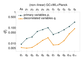
All errors are shown in the left panel of Figure 13. Notice how in this case, the improvement on the errors of the $q_{i}$ variables is less than an order of magnitude, thus smaller than what found in GC and WL separately; this is due to combination of GC and WL which, together with the inclusion of the CMB prior, lead to smaller correlations among the parameters. When combining GC+WL in the non-linear HS case, the FoC (defined in 29) is $\approx 31$, showing that there is not much gain in decorrelation, compared to GC or WL alone, where this quantity was approximately $32$. However, combining GC+WL (non-linear HS) with Planck priors yields $\textrm{FoC}\approx 22$, showing that correlations among parameters are drastically reduced. The fact that the curve of 1$\sigma$ errors for the $q_{i}$ (orange line, marked with circles) follows the same pattern as the curve for the $p_{i}$ errors (green dashed line, marled with circles), is due to the fact that we have used a ZCA decomposition and therefore the $q_{i}$ are as close as possible to the $p_{i}$. The complete matrix of coefficients $W$ can be found in Table 15 in appendix D.

Figure 13: Left: the 1$\sigma$ fully marginalized errors on the primary parameters $p_{i}$ (green dashed lines), and the 1$\sigma$ errors on the decorrelated derived parameters $q_{i}$ (yellow solid lines). As opposed to the GC or WL cases (figs.7,10), here the decorrelated errors are much more similar to the standard errors. This is due to the fact that in the GC+WL+Planck combination, the cosmological parameters are not so strongly correlated. Right: best constrained modes for a Euclid Redbook GC+WL case using the non-linear HS prescription and adding a CMB Planck prior. Each panel shows the four best constrained parameters $q_{i}$. Each of them is a linear combination of the primary parameters $p_{i}$. The best constrained modes are sums $a\mu_{i}+b\eta_{i}$ for $i=\{1,2,3\}$ and positive values $a$ and $b$.

VI Modified gravity with simple smooth functions of the scale factor

As discussed in Sec. II, $\mu$ and $\eta$ (or an equivalent pair of functions of the gravitational potentials) depend in general on time and space. We will now investigate the time dependence further, starting from the two parameterizations proposed in Planck Collaboration et al. (2016) and recalled in Eqns. (9-12) in this paper. We extend the analysis of the Planck paper by testing different prescriptions for the non-linear regime in Modified Gravity (as illustrated in Section III) and further investigate forecasts for future experiments like Euclid, SKA, DESI. In the following subsections we first give results for the late-time parameterization of Eqns. (9,10) and then for the early time parameterization of Eqns. (11,12). In both cases we consider Galaxy Clustering and Weak Lensing, neglecting, as in Section V any information coming from the cross correlation of the two probes.

VI.1 Modified Gravity in the late-time parameterization

The late-time parameterization is defined in Eqns. (9,10). We now calculate forecasts for Galaxy Clustering and Weak Lensing, with future surveys, in the linear and mildly non-linear regimes. We also include prior information obtained from the analysis of the Planck+BSH datasets (where we recall that BSH stands for BAO + SNe + $H_{0}$ prior), as discussed in Section IV.5.

VI.1.1 Galaxy Clustering in the linear and mildly non-linear regime

In Table VI.1.1 we show forecasts for the Euclid survey Laureijs and others (2011) for Galaxy Clustering (top part of the table) and three different cases: using only linear scales with a cutoff at $k_{\rm max}=0.15$h/Mpc, labeled GC(lin); extending forecasts in the mildly non-linear regime, obtained using the prescription described in Sec. III.2.2, with a cutoff at $k_{\rm max}=0.5$ h/Mpc, labeled GC(nl-HS); combining the mildly non-linear case with Planck priors, as described in Sec. IV.5. We take into account the BAO features, redshift space distortions and the full shape of the power spectrum, as well as the survey specifications of the Euclid Redbook, recalled in Section IV.2 for convenience. The columns correspond to the marginalized errors on five standard cosmological parameters $\{\Omega_{c},\Omega_{b},n_{s},\ln(10^{10}A_{s}),h\}$ and three combinations of the gravitational potentials $\{\mu,\eta,\Sigma\}$: the latter are reconstructed in time, according to the late-time parameterization, as defined in Eqns. (9,10). We recall that only two of these three functions are independent and fully determine cosmological linear perturbations.

In the late-time scenario, for a Galaxy Clustering survey, neither $\eta$ nor $\Sigma$ are actually constrained by a linear forecast, while $\mu$ is mildly constrained. Adding the non-linear regime improves constraints on $\mu$, while the other parameters remain unconstrained, unless we also include Planck priors, which yields an improvement in the FoM of 6.3 nits. In general the observable power spectrum may depend on both $\mu$ (explicitely appearing in the last term of the equation for the density perturbation (cf. Eqn.(61)) and on $\eta$ (implicitly contained in the derivatives of the gravitational potential in the same equation). The contribution of the derivative of the potentials is larger in the early-time parameterization, with respect to the late-time one by construction. This is due to the fact that in the late-time case deviations from GR go to zero at large redshifts. In this sense, in the specific case of the late time parameterization, the observed power spectrum mainly depends on $\mu$ only, which explains why this is the only quantity (mildly) constrained by GC alone. In the early-time parameterization, though, modifications can appear also at earlier times, so that both $\eta$ and $\mu$ effectively affect the power spectrum, which explains why they can both be constrained with a smaller uncertainty, as we will discuss in Section VI.2.

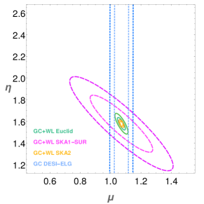
In Appendix B we review the equation governing the evolution of cold dark matter density fluctuations, as a function of the Modified Gravity functions $\mu(a)$ and $\eta(a)$ as they are implemented in the code MGCAMB Hojjati et al. (2011). The inability of GC to constrain $\eta$ in this parametrization, is also visible in Fig. 14 which shows that the GC constraints are degenerate along the $\eta$ or $\Sigma$ directions. Therefore, we show how with this parameterization choice Euclid GC will be extremely sensitive to modifications of the Poisson equation for $\Psi$, while it would require additional information to constrain departures from the standard Weyl potential.

Table 5: 1$\sigma$ fully marginalized errors on the cosmological parameters in the late-time parameterization of Modified Gravity for a Euclid Galaxy Clustering forecast (top), a Weak Lensing forecast (middle) and the combination of both probes (bottom): Modified Gravity is encoded in two of the three functions $\mu$, $\eta$, $\Sigma$, which are reconstructed in the late-time parameterization defined in Eqns. (9,10). For each case, we also list the forecasted errors using a Planck+BSH prior. Linear forecasts are labeled by “lin”, and correspond to a cutoff $k_{\rm max}=0.15$h/Mpc for GC and $\ell_{\rm max}=5000$ for WL; non-linear forecasts use the prescription described in sec. III.2.2, are labeled by “nl-HS” and correspond to a cutoff of $k_{\rm max}=0.5$h/Mpc for GC and $\ell_{\rm max}=5000$ for WL. in both cases, power spectra have been computed using the MGCAMB Boltzmann code. For completeness, we also show the GC+WL+Planck case using the non-linear power spectra computed using Halofit only (nl-Halofit). In the last column, we show for each observation the Figure of Merit (FoM) relative to our base observable in this parametrization, which is GC(linear). GC(linear) has an absolute FoM of -0.94 in ‘nits’. We can see that in both GC and WL there is a considerable gain when including non-linear scales and Planck priors. The difference in the FoM between the non-linear HS prescription and the standard Halofit approach is quite small.

& 0 GC(nl-HS) 0.9% 2.5% 1.3% 0.8% 1.7% 1.7% 475% 291% 2.9 GC(nl-HS)+Planck 0.7% 0.6% 0.3% 0.2% 0.3% 1.7% 16.8% 10.3% 6.3 WL(lin) 7.8% 25.7% 9.9% 10.3% 19.1% 58.2% 106% 9.3% 3.2 WL(nl-HS) 6.3% 20.7% 4.6% 5.8% 13.8% 23.3% 40.9% 4.6% 4.5 WL(nl-HS)+Planck 2.1% 1.1% 0.4% 0.7% 0.7% 11.8% 21.8% 2.8% 5.7 GC+WL(lin) 1.8% 5.9% 2.8% 2.3% 4.2% 7.1% 10.6% 2% 6.6 GC+WL(lin)+Planck   1.0% 0.7% 0.4% 0.4% 0.4% 6.2% 9.8% 1.5% 7.0 GC+WL(nl-HS) 0.8% 2.2% 0.8% 0.7% 1.5% 1.6% 2.4% 1.0% 8.8 GC+WL(nl-HS)+Planck   0.7% 0.6% 0.2% 0.2% 0.3% 1.6% 2.4% 0.9% 8.9 GC+WL(nl-Halofit)+Planck   0.6% 0.5% 0.2% 0.2% 0.2% 0.8% 1.7% 0.8% 9.6

Table 6: Same as Table (VI.1.1) but for the early-time parameterization. Note that the last column (MG FoM) cannot be compared to the one for a different parameterization (Table VI.1.1) since the reference value is different (GC(lin)) and the two parameterizations have a different number of primary parameters). In this case the absolute MG FoM of GC(lin) is $\approx-0.47$ nits.

& 0 GC(nl-HS) 1.1% 2.3% 1.3% 0.7% 1.6% 1.8% 7.9% 4.8% 6.6 GC(nl-HS)+Planck 0.8% 0.7% 0.3% 0.3% 0.3% 1.7% 7.6% 4.6% 6.7 WL(lin) 12.1% 28.9% 11.3% 13.3% 24% 6.8% 11.1% 11.9% 4.9 WL(nl-HS) 6.5% 21.9% 6.6% 5.9% 15.8% 2.8% 8.0% 3.4% 6.6 WL(nl-HS)+Planck 2.1% 1.3% 0.5% 0.9% 0.7% 2.2% 7.2% 2.9% 7.2 GC+WL(lin) 1.8% 6.6% 3.4% 5.6% 5.2% 3.0% 6.8% 3.4% 6.4 GC+WL(lin)+Planck 1.2% 0.9% 0.6% 2.3% 0.4% 2.4% 6.5% 2.8% 6.9 GC+WL(nl-HS) 1.0% 2.2% 1.2% 0.7% 1.6% 1.3% 4.4% 1.9% 8.0 GC+WL(nl-HS)+Planck 0.8% 0.7% 0.3% 0.3% 0.3% 1.3% 4.4% 1.9% 8.2 GC+WL(nl-Halofit)+Planck   0.7% 0.7% 0.3% 1.3% 0.3% 0.9% 2.3% 1% 8.9

Table 7: 1$\sigma$ fully marginalized errors on the cosmological parameters $\{\Omega_{m},\Omega_{b},h,\ell\mathcal{A}_{s},n_{s},\mu,\eta,\Sigma\}$ in the late-time parameterization comparing different surveys in the linear and non-linear case. In the last column, we show for each observation the Modified Gravity Figure of Merit (MG FoM) relative to our base observable, which is the Euclid Redbook GC(linear), see Table VI.1.1. We can see that in general terms, SKA2 is the most powerful survey, followed by Euclid and SKA1. In the case of GC alone, DESI-ELG is more constraining than SKA1-SUR. Notice that in this parameterization, a GC survey would only constrain $\mu$ with a high accuracy, while a WL survey would constrain $\Sigma$ with a very good accuracy. The combination of both is much more powerful than the single probes. Adding Planck priors (last row) improves considerably the constraints on the $\Lambda\mathrm{CDM}$ parameters but has an almost negligible effect on the MG parameters (MG FoM remain almost constant when adding Planck priors to the GC+WL (non-linear HS) case. The marginalized contours for the $\mu$-$\eta$ plane , comparing these surveys, can be seen in the left panel ofFig.16.

& 2.9 SKA1-SUR 5% 15.3% 8.7% 3.8% 10.8% 18.1% 165% 108% 1.7 SKA2 0.5% 1.3% 0.4% 0.4% 0.8% 0.7% 86.8% 53.2% 5.5 DESI-ELG 1.6% 4.1% 2.3% 1.3% 2.9% 3.3% 899% 552% 1.8 WL(nl-HS) Euclid 6.3% 20.7% 4.6% 5.8% 13.8% 23.3% 40.9% 4.6% 4.5 SKA1 30.8% 109% 35% 36.5% 77.6% 220% 405% 36.8% 0.5 SKA2 6% 22.5% 5.9% 6.8% 15.9% 19% 33.2% 3.7% 4.9 GC+WL(lin) Euclid 1.8% 5.9% 2.8% 2.3% 4.2% 7.1% 10.6% 2% 6.6 SKA1 10.1% 47.6% 25.4% 21.7% 40.4% 26.4% 28.8% 13.6% 3.7 SKA2 1.2% 4.5% 2.2% 1.9% 3.3% 4.1% 5.5% 1.6% 7.5 GC+WL(lin)+Planck Euclid 1.0% 0.7% 0.4% 0.4% 0.4% 6.2% 9.8% 1.5% 6.9 SKA1 2.4% 1.2% 0.4% 1.2% 0.7% 12% 19.8% 3.8% 5.3 SKA2 0.7% 0.6% 0.3% 0.4% 0.3% 3.6% 5.2% 1.2% 7.8 GC+WL(nl-HS) Euclid 0.8% 2.2% 0.8% 0.7% 1.5% 1.6% 2.4% 1.0% 8.7 SKA1 4.7% 14.3% 6.2% 3.6% 9.6% 12.8% 11% 7.3% 5.5 SKA2 0.4% 1.3% 0.3% 0.4% 0.8% 0.7% 0.9% 0.6% 10.3 GC+WL(nl-HS)+Planck Euclid 0.7% 0.6% 0.2% 0.2% 0.3% 1.6% 2.4% 0.9% 8.9 SKA1 2.0% 1.0% 0.4% 0.8% 0.6% 3.5% 6% 2.7% 6.9 SKA2 0.4% 0.5% 0.2% 0.1% 0.2% 0.6% 0.9% 0.5% 10.3

& 6.6 SKA1-SUR 7.9% 14.2% 13.4% 4.2% 11% 12.6% 82.7% 52.6% 2.2 SKA2 0.6% 1.3% 0.7% 0.4% 0.9% 0.9% 3.4% 1.8% 8.3 DESI-ELG 2.0% 4.3% 2.7% 1.4% 3.0% 8.2% 32% 28.6% 4.3 WL(nl-HS) Euclid 6.5% 21.9% 6.6% 5.9% 15.8% 2.8% 8.0% 3.4% 6.6 SKA1 32% 106% 37.2% 33% 79.3% 13.1% 37.1% 16.4% 3.4 SKA2 5.9% 22.1% 6.7% 6.1% 16.1% 2.4% 7.0% 2.9% 6.9 GC+WL(lin) Euclid 1.8% 6.6% 3.4% 5.6% 5.2% 3.0% 6.8% 3.4% 6.4 SKA1 10.3% 46.4% 24.2% 33.6% 40.2% 14.4% 29.6% 15.5% 3.3 SKA2 1.3% 4.9% 2.5% 4.2% 3.9% 2.5% 5.7% 2.7% 6.8 GC+WL(lin)+Planck Euclid 1.2% 0.9% 0.6% 2.3% 0.4% 2.4% 6.5% 2.8% 6.8 SKA1 2.5% 1.5% 0.8% 2.9% 0.8% 8.8% 22.2% 8.5% 4.5 SKA2 0.9% 0.7% 0.6% 2.1% 0.3% 2.1% 5.4% 2.3% 7.2 GC+WL(nl-HS) Euclid 1.0% 2.2% 1.2% 0.7% 1.6% 1.3% 4.4% 1.9% 8.1 SKA1 7.1% 13.4% 10.7% 4% 10% 8.2% 24.4% 10.5% 4.4 SKA2 0.6% 1.3% 0.7% 0.4% 0.9% 0.8% 2.7% 1.3% 8.8 GC+WL(nl-HS)+Planck Euclid 0.8% 0.7% 0.3% 0.3% 0.3% 1.3% 4.4% 1.9% 8.1 SKA1 2.1% 1.3% 0.5% 0.9% 0.7% 7% 20.8% 8.2% 4.9 SKA2 0.5% 0.5% 0.3% 0.2% 0.2% 0.8% 2.7% 1.3% 8.8

VI.1.2 Weak Lensing in the linear and mildly non-linear regime

Using the Euclid Weak Lensing specifications described in Section sub:Fisher-Weak-Lensing, we obtain the results displayed in the middle panel of Table VI.1.1. Also in this case, we use the late-time parameterization, in three different cases: the first uses only linear quantities, with a maximum multipole of $\ell_{\rm max}=1000$; the second case uses the non-linear HS prescription of section III.2.2 up to a maximum multipole of $\ell_{\rm max}=5000$; the third case combines Weak Lensing with Planck priors, as described in IV.5.

In the linear case, WL forecast yields constraints on the standard $\Lambda\mathrm{CDM}$ parameters at around 10% of accuracy, with the exception of $\Omega_{b}$ which is poorly constrained at around 26%, and the expansion rate h (19%). This is likely due to the fact that WL is only directly sensitive to the total matter distribution in the Universe and cannot differentiate baryons from dark matter. All constraints improve when adding non-linear information, with $\Omega_{b}$ and h still constrained only at the level of about $20\%$. When the Planck priors are included, though, constraints shrink down to about 1$\%$ for all cosmological parameters. The Modified Gravity parameters show the expected trend; in the linear case, only $\Sigma$ is constrained, at 11$\%$, as this parameter is directly defined in terms of the lensing potential $\Phi+\Psi$; a Weak Lensing probe is however not directly sensitive to $\mu$ and $\eta$ separately, as can be seen in Fig. 14. The linear FoM is only slightly weaker than the one from GC for this parameterization, probably because both probes have an effectively unconstrained degeneracy direction. When adding non-linear information, errors on $\mu$ and $\eta$ improve, though still remaining in a poorly constrained interval (25$\%$-44$\%$). Already on its own, however, Weak Lensing could rule out many models of Modified Gravity that change $\Sigma$ at more than $5\%$ (or even $2.9\%$, if we include Planck priors). The combination GC+Planck and WL+Planck has a comparable overall constraining power, with GC+Planck being about 1 nit stronger and providing smaller errors on $\mu$.

VI.1.3 Combining Weak Lensing and Galaxy Clustering

Figure 14: Fisher Matrix marginalized contours (1, 2 $\sigma$) for the Euclid space mission in the late-time parameterization using mildly non-linear scales and the HS prescription. Green lines represent constraints from a Galaxy Clustering survey, pink lines stand for the Weak Lensing observables, and orange lines represent the GC+WL+Planck combined confidence regions. Upper Left: contours for the fully marginalized errors on $\eta$ and $\mu$. Upper Right: contours for the fully marginalized errors on $\Sigma$ and $\mu$. Lower Left: contours for the fully marginalized errors on $\mu$ and $\Omega_{b}$. Lower Right: contours for the fully marginalized errors on $\Sigma$ and $\ln(10^{1}0A_{s})$. The fact that the combination of GC, WL and Planck breaks many degeneracies in the 7-dimensional parameter space, explains why the combined contours (yellow) have a much smaller area. Notice that in this parametrization, GC measures mostly $\mu$ and WL constrains mostly just $\Sigma$.

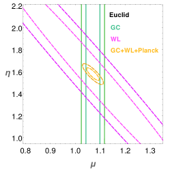
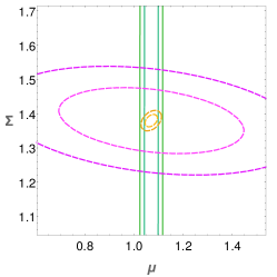
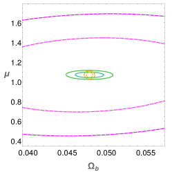
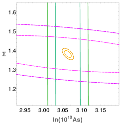
After using the two primary probes from Euclid separately, we discuss here the constraints obtained combining Weak Lensing and Galaxy Clustering. The combination between GC and WL can be seen in the bottom panel of Table VI.1.1. In the late-time parameterization, in the linear case, Weak Lensing combined with a galaxy clustering for a Euclid survey (Redbook specifications) constrains the standard $\Lambda$CDM parameters in the range $2\%-6\%$, and below 1$\%$ when Planck priors are included. Modified Gravity parameters $\mu$ and $\eta$ are now also constrained below 10$\%$, reaching $1\%$ when adding non-linear scales. The remarkable improvement can be attributed to the fact that the combination of GC and WL Fisher matrices breaks many degeneracies in the parameter space. This is shown in Figure 14, where it is possible to notice how the two probes are almost orthogonal both in the $\mu$-$\eta$- and $\mu$-$\Sigma$-plane. Weak Lensing measures the changes in the Weyl potential, parametrized by $\Sigma$, while $\mu$ is related to the Poisson equation, and therefore to the potential $\Psi$, modified by peculiar velocities and sensitive to Galaxy Clustering; $\eta$ can also be written as a combination of $\mu$ and $\Sigma$ (see Eqn. 5).

Further improvement is brought by the sensitivity of Galaxy Clustering to standard $\Lambda$CDM parameters; even though GC constraints on $\Sigma$ and $\eta$ are not as good as the ones for Weak Lensing, the better measurement of standard parameters provided by Galaxy Clustering breaks degeneracies in the Modified Gravity sector of the parameter space, leading to narrower bounds for $\eta$ and $\Sigma$ with respect to both probes taken separately. WL is instead not sensitive to modifications of the Poisson equation for matter and this explains why constraints on $\mu$ are not improved by the combination of the two probes, but are rather dominated by GC. The correlation among parameters can also help us explain the observed results. The Figure of Correlation, defined in Eq. (29), for GC (non-linear HS) alone is 4.9, while for WL (non-linear HS) the correlation is higher, with $\textrm{FoC}=16.9$. When combining both probes (GC+WL (non-linear HS)) the FoC goes to an intermediate point of 7.6.

Given the constraining power of the GC+WL combination on MG functions, adding the Planck priors does not lead to significant improvements on the dark energy related parameters. On the other hand, standard parameters significantly benefit from the inclusion of CMB and background priors and we can expect this to be a relevant factor for MG models with degeneracies with $\Lambda$CDM parameters, e.g. models affecting also the expansion history of the universe. An overview of the constraints on Modified Gravity described in this section is shown in Fig.14, with Euclid GC, Euclid WL and Euclid GC+WL combined with Planck priors.

VI.1.4 Forecasts in Modified Gravity for SKA1, SKA2 and DESI

Figure 15: 1$\sigma$ fully marginalized errors on the parameters $\{\Omega_{m},\Omega_{b},h,\ell\mathcal{A}_{s},n_{s},\mu,\eta,\Sigma\}$ for the late-time parameterization of MG obtained by forecasts on Galaxy Clustering (non-linear HS) (top left panel), Weak Lensing (non-linear HS) (top right panel), the combinations GC+WL (linear) (middle left) and GC+WL+Planck (linear) (middle right) and the combinations GC+WL (non-linear HS) (bottom left) and GC+WL+Planck (non-linear) (bottom right). In the GC case, the surveys considered are SKA2 (blue), SKA1-SUR (green), Euclid Redbook (purple) and DESI-ELG (orange). For forecasts including WL, only Euclid, SKA1 and SKA2 are included. Although the 1$\sigma$ constraints on the standard parameters are overall weaker for WL than for GC, Weak Lensing surveys perform better on Modified Gravity parameters. Comparing the different surveys, Euclid and SKA2 perform similarly well for the WL observable alone, if non-linearities are included. Notice that SKA1-SUR performs better than Euclid on the $\eta$ and $\Sigma$ parameters, because it can measure better at lower redshifts. Including the Planck prior, the GC+WL combination for Euclid and SKA2 constrains all parameters at much better than percent accuracy. Detailed specifications of the different surveys are explained in the text.

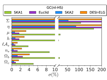
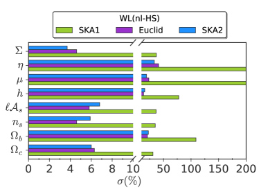
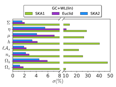
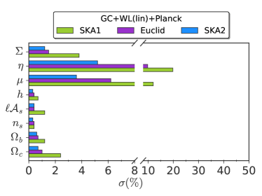
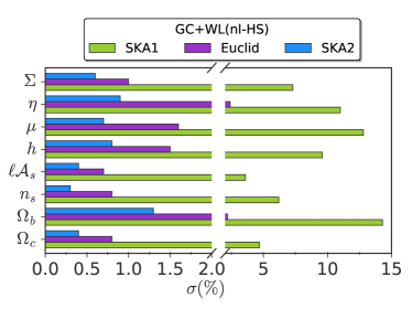
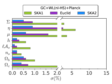
For the SKA1 and SKA2 surveys (whose specifications are explained in detail in Section IV.1), previous work on forecasting cosmological parameters has been done, among others, by Baker and Bull (2015) and Bull (2015). In the latter work, the author parameterizes the evolution of $\mu(a)$ using the late-time parameterization, but also adds an extra parameter allowing for a scale dependence in $\mu(a)$ and including a Planck prior. For a fixed scale, the 1$\sigma$ errors on the amplitude of $\mu$ lie between 0.045 and 0.095, depending on the details of the SKA1 specifications, while for SKA2, this error is of about 0.017. This setting would correspond to our GC+WL(linear) + Planck case (see Table VI.1.1) where we find for SKA1 a 1$\sigma$ error on $\mu$ of 0.12 and for SKA2 the forecasted error is 0.036. Our errors are somewhat larger, but we also have extended our analysis to let the gravitational slip $\eta$ be different from 1 at present time, our departure from $\mu=1$ at present time is larger by a factor 4 and our linear forecast is conservative in the sense that it includes less wavenumbers $k$ at higher redshifts, compared to theirs.

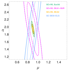
In Figure 15 we show the 1$\sigma$ fully marginalized forecasted errors on the parameters $\{\Omega_{m},\Omega_{b},h,\ell\mathcal{A}_{s},n_{s},\mu,\Sigma\}$ for different Weak Lensing (left panel) and Galaxy Clustering (right panel) surveys in the late-time parameterization. In the GC case, the surveys considered are DESI-ELG (yellow), SKA2 (green), SKA1-SUR (orange) and Euclid (blue). For the WL forecast, we considered Euclid (blue), SKA1 (orange) and SKA2 (green). These constraints correspond to the ones listed in Table VI.1.1. The marginalized confidence contours for the $\mu$-$\eta$ plane , comparing all these surveys, can be seen in the left panel ofFig.16. The 1$\sigma$ fully marginalized constraints on the parameters are weaker for WL than for GC, which may be a consequence of the higher correlation among variables for the Weak Lensing observable, described in the previous section VI.1.3. Comparing the different surveys, the general trend is that Euclid and SKA2 perform at a similar level for WL at both linear and non-linear level; for GC and when combining both probes, SKA2 gives the strongest constraints, followed by Euclid, SKA1 and DESI (for GC). Notice that in this parameterization, a SKA1-SUR GC survey constrains the $\Sigma$ parameter alone better than a Euclid Galaxy Clustering survey (although Euclid is overall much stronger as can be seen with the FoM). This is due to the fact that SKA1-SUR probes much lower redshifts (from $z=0.05-0.85$) than Euclid and is therefore suitable to better constrain those parameterizations in which the effect of the Modified Gravity parameters is stronger at lower redshifts; this is the case of the late-time parameterization, which is proportional to the dark energy density, dominating at low redshifts only. This result is reversed in the early time parameterization, in which Modified Gravity can play a role also at earlier redshifts.

Figure 16: 1$\sigma$ and 2$\sigma$ fully marginalized confidence contours on the parameters $\mu$ and $\eta$, for 3 different surveys combining Galaxy Clustering (GC) and Weak Lensing (WL): Euclid, SKA1-SUR and SKA2 and for GC only: DESI-ELG, all in the late-time (left panel) and early-time (right panel) parameterizations of sections VI.1 and VI.2, respectively. As explained in the main text, the constraints are parameterization-dependent, especially on $\eta$, where in the late-time scenario GC alone is not able to constrain it, while in the early-time scenario GC can constrain both $\mu$ and $\eta$.

VI.2 Modified Gravity in the early-time parameterization

VI.2.1 Galaxy Clustering, Weak Lensing and its combination

We extend our analysis now to an alternative choice, the early time parameterization specified in Eqns. (11) and (12). As before, we use Euclid Redbook specifications for WL and GC and the cut in scales discussed previously for the two observables, i.e. a maximum wavelength cutoff at $k_{\rm max}=0.15$ for GC and a maximum multipole of $\ell_{\rm max}=1000$ for WL in the linear case, and a cutoff $k_{\rm max}=0.5$h/Mpc and a maximum multipole of $\ell_{\rm max}=5000$ for WL in the non-linear regime, which is analyzed using the prescription described in Sec. III.2.2. We use the two observables both separately and in combination, without accounting for cross correlation of the two (as discussed in section V this seems to correspond to a conservative choice), with and without Planck priors.

Results are shown in Table VI.1.1 and Figure V.1. The general behaviour of the constraints is similar to the one in the late-time parameterization, with the combination of GC and WL able to break the degeneracies with standard cosmological parameters, leading to a significant improvement of the constraints on MG parameters, constraining $\mu$ and $\Sigma$ at the 1-2% level. There are some other interesting differences with the late-time scenario. First, the addition of Planck priors does not really improve much the constraints obtained by GC or WL alone, which was not the case in the late-time parametrization. This is related to the fact that in the early-time parameterization, GC and WL (non-linear) on their own are already good at constraining both $\mu$ (at 2-3 %) and $\eta$ (at around 8%), with consequently small errors on $\Sigma$ ($\approx 3$%). In Appendix B we show the derivatives of the matter power spectrum with respect to the MG parameters $\mu$ and $\eta$ in both parameterizations. We can observe that in the early-time scenario, the derivative $dP(k)/d\eta$ is larger than in the late-time parameterization, leading therefore to better constraints. Another difference lies in the correlation among parameters, which for WL and GC+WL is considerably smaller than in the late-time scenario. The Figure of Correlation (defined in Eqn. 29) for GC (non-linear HS) alone is 4.7, while for WL (non-linear HS) the correlation is somewhat higher, with $\textrm{FoC}=7.3$. When combining both probes (GC+WL (non-linear HS)) the FoC goes to an intermediate point of 5.2.

Table 8: Same as Table VI.1.1 but for the early-time parameterization. The last 4 columns correspond to the projection of the errors on $E_{11}$ and $E_{22}$ onto $\mu,\;\eta$ and $\Sigma$, respectively. We have marginalized over $E_{12}$ and $E_{21}$ since at $z=0$ they don’t contribute to the Modified Gravity parameters. Notice that in this parameterization, a GC survey alone is able to constrain both $\mu$ and $\Sigma$ to a good level for all surveys, better than with the late time parameterization, more often used in literature. The combination of GC+WL is however less constraining in the early time parametrization than in late time parameterization one. The reference case for the MG FoM is the Euclid (Redbook) GC linear forecast (Table VI.1.1). The non-linear forecast for GC+WL+Planck would yield, for Euclid and SKA2, contraints at the 1-2% accuracy on $\mu$, $\Sigma$, while for SKA1 the contraints would be at the 8% level. The marginalized contours for the $\mu$-$\eta$ plane , comparing these surveys, can be seen in the right panel ofFig.16.

Figure 17: Fisher Matrix marginalized forecasted contours (1$\sigma$, 2$\sigma$) for the Euclid Redbook satellite in the early-time parameterization using mildly non-linear scales and the HS prescription. Green lines represent constraints from the Galaxy Clustering survey, pink lines stand for the Weak Lensing observables, and orange lines represent the GC+WL+Planck combined confidence regions. Upper left: contours for the fully marginalized errors on $\eta$ and $\mu$. Upper right: contours for the fully marginalized errors on $\Sigma$ and $\mu$. Lower left: contours for the fully marginalized errors on $\mu$ and $\Omega_{b}$. Lower right: contours for the fully marginalized errors on $\Sigma$ and $\ln 10^{10}A_{s}$. Notice that in this parameterization, GC and WL are able to constrain both $\mu$ and $\eta$ or $\Sigma$ on their own.

VI.2.2 Other Surveys: DESI-ELG, SKA1 and SKA2

Also in the early time parameterization we obtain the 1-$\sigma$ fully marginalized errors for Galaxy Clustering (top left panel of Figure 18) considering DESI-ELG (yellow), SKA2 (green), SKA1-SUR (orange) and Euclid (blue), and for Weak Lensing (top right panel of Figure 18) using Euclid (blue), SKA1 (orange) and SKA2 (green). We also report the results in Table V.1, where it is possible to notice how the conclusions drawn on the hierarchy of the considered experiments do not change with respect to the late-time parameterization. The main difference is that in this case the full SKA1-SUR GC survey does not constrain the $\Sigma$ parameter better than the Euclid survey; this is due to the fact that in the early time parametrization, deviations from $\Lambda$CDM are present also at high redshift, therefore we do expect the information present at small redshift to be as relevant as the one coming from higher $z$, where Euclid performs significantly better than SKA1-SUR. The marginalized contours for the $\mu$-$\eta$ plane, comparing all these surveys, can be seen in the right panel of Fig.16.

Figure 18: Same as Fig.15 but for the early-time parameterization (Eqns. 11,12) The 1$\sigma$ fully marginalized constraints on the parameters are weaker for WL than for GC, which is a consequence of the higher correlation among variables for the Weak Lensing observable.

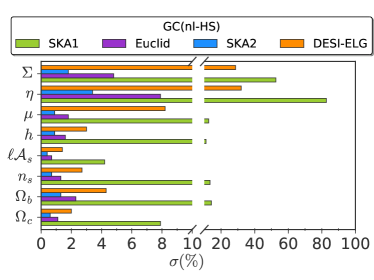
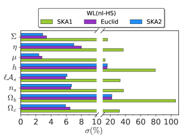
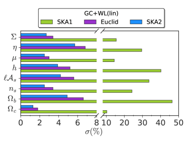
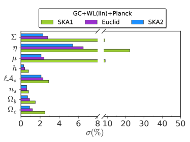
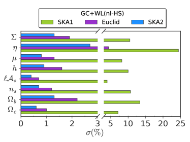
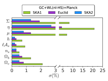
VI.3 Testing the effect of the Hu-Sawicki non-linear prescription on parameter estimation

In this section we show the effect of changing the parameters $c_{\mathrm{nl}}$ and $s$ used in the HS prescription (specified in Eq. 13) for the mildly non-linear matter power spectrum. As mentioned already in Section III.2.2, previous works (see Zhao (2014); Zhao et al. (2011); Koyama et al. (2009)), have fitted the values of $c_{\mathrm{nl}}$ and $s$ to match N-body simulations in specific Modified Gravity models. In all these cases the HS parameters $c_{\mathrm{nl}}$ and $s$ have been found to be of order unity, with $c_{\mathrm{nl}}$ ranging usually from $0.1$ to $3$ and $s$ from about $1/3$ to a value of around $2$. In the absence of N-body simulations for our models, we selected our benchmark HS parameters to be $c_{\mathrm{nl}}=1$ and $s=1$, as discussed in Section III.2.2, which we used for all the analysis presented above. However, in order to test the effect of a change of $c_{nl}$ and $s$ non-linear parameters on our estimation of errors on the cosmological parameters, we perform our GC and WL forecasts on the MG late-time model (Section VI.1) also changing one at a time the values of both HS parameters. We use the following values for our test: $c_{\mathrm{nl}}=\{0.1,0.5,\,1,\,3\}$ and $s=\{0,\,1/3,\,2/3,\,1\}$.

Figure 19: Effect of the $c_{\mathrm{nl}}$ and $s$ parameters on the 1$\sigma$ marginalized error of the $\mu$ (left panel) and the $\eta$ (right panel) parameters in the MG late-time parametrization for a Euclid Galaxy Clustering forecast with Redbook specifications. The colored contours show the percentage discrepancy when departing from the benchmark case $c_{\mathrm{nl}}=1$ and $s=1$ (marked with a black arrow) to all other points in the $c_{\mathrm{nl}}$-$s$ space. The red (blue) contours signal the regions of maximum positive (negative) discrepancy. For example in the left panel, choosing $c_{\mathrm{nl}}$ and $s$ in the red region, will yield a 1$\sigma$ marginalized error on $\mu$ which is 90% larger than in the benchmark case (see Table VI.1.1 for the benchmark forecast). For the standard $\Lambda\mathrm{CDM}$ cosmological parameters (not shown here) the discrepancy is smaller than 4% for all choices of $c_{\mathrm{nl}}$ and $s$.

Figure 20: Same as Fig.19 but for a Weak Lensing Euclid forecast using Redbook specifications. In the left panel, choosing $c_{\mathrm{nl}}$ and $s$ in the red region, will yield a 1$\sigma$ marginalized error on $\mu$ which is 60% larger than in the benchmark case (see Table VI.1.1 for the benchmark forecast). In the right panel we see that for the MG parameter $\Sigma$ the maximum positive and negative discrepancy is only of about 6%. The maximum and minimun discrepancy for the MG parameter $\eta$ is of -15% and 50%. This means that the parameter $\Sigma$ (defined as the lensing Weyl potential, and therefore directly constrained by Weak Lensing) is much less sensitive to changes in the non-linear prescription parameters.

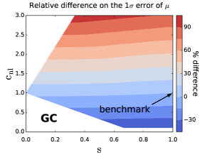
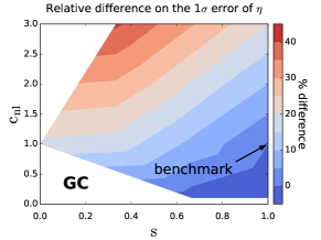
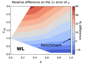
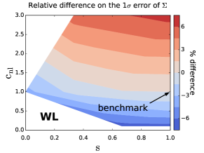
In Figure 19 we show the percentage discrepancy between the 1$\sigma$ marginalized error obtained on parameters in the GC non-linear HS benchmark case (see Table VI.1.1 for the exact values) and the corresponding error obtained by performing the same forecast with a different value of the $c_{\mathrm{nl}}$-$s$ parameters. In general terms we see that for the MG parameter $\mu$ (left panel of Figure 19) the relative difference in the estimation of the 1$\sigma$ forecasted errors can lie between 90% (at $c_{\mathrm{nl}}=3$, $s=0.33$) and -30% for $c_{\mathrm{nl}}=0.1$ and $s=1.0$. The behavior of the contour lines shows us that for a fixed value of $c_{\mathrm{nl}}$, the forecasted error on the parameter $\mu$ remains unaffected. For $\eta$ (right panel) the relative discrepancy lies between 40% and -2%. Here, to get the same 1$\sigma$ errors on $\eta$, one would have to vary both $c_{\mathrm{nl}}$ and $s$. We also tested the effect on the standard $\Lambda\mathrm{CDM}$ parameters and found it to be smaller than 4% for all choices of $c_{\mathrm{nl}}$ and $s$. In the case of WL forecasts, we perform the same tests, which are shown in Figure 20. We can observe that the relative discrepancies in the case of the $\mu$ parameter lie between $\sim$60% and $\sim$-15%, while for $\Sigma$ the discrepancy is considerably smaller. The 1$\sigma$ error on $\Sigma$ varies only between $\pm 6$%. This is however a particular effect of choosing $\Sigma$, which is the true WL observable. If we perform this test on $\eta$ using WL, we will find a stronger discrepancy, that lies in between $\sim$50% and $\sim$-15%, similar to the one found for $\mu$.

We can also test the effect of adding these two HS parameters as extra nuisance parameters to our model of the non-linear power spectrum; therefore, by taking derivatives of the observed power spectrum with respect to these parameters, we can forecast what would be the estimated error on $c_{\mathrm{nl}}$ and $s$. Then, marginalizing over $c_{\mathrm{nl}}$ and $s$ would yield more realistic constraints on our cosmological parameters, and take into account our ignorance on the correct parameters of the HS prescription. In Table VI.3 we list the 1$\sigma$ marginalized constraints on $c_{\mathrm{nl}}$ and $s$ for our benchmark fiducial ( $c_{\mathrm{nl}}=1$, $s=1$) and using the standard fiducial for the cosmological parameters used previously for the MG late time parametrization.

Taking these HS parameters into account in our Fisher forecast, will automatically change the constraints on the other parameters. For our method to be consistent, we would like this effect to remain as small as possible. In Table VI.3, we list the same constraints reported in Table VI.1.1, but obtained marginalizing over $c_{\mathrm{nl}}$ and $s$ at the benchmark fiducial $c_{\mathrm{nl}}=1$, $s=1$. Comparing the two tables, we can see that for GC the errors on the cosmological parameters remain quite stable, except for $\eta$ and $\Sigma$; this is understandable since those parameters are not well constrained by GC alone. For WL, we see a difference of 4 to 7 percent points in the errors on $h$, $n_{s}$ and $\Omega_{b}$, while all other errors remain stable, with $\Sigma$ varying less than 2 percent points. Remarkably, the combined constraints from GC+WL are even less affected by the two nuisance parameters. Comparing the Modified Gravity FoM between the two tables, shows the expected behavior, the MG FoM is reduced when adding two extra parameters, but the change is very small, of just 0.3-0.5 nits.

Table 9: 1-$\sigma$ fully marginalized errors on the cosmological parameters and the two HS parameters $c_{\mathrm{nl}}$ and $s$ for a Euclid Galaxy Clustering forecast, a Weak Lensing forecast and the combination of both in the late-time parameterization of Modified Gravity using non-linear scales and the HS prescription. In contrast to Table VI.1.1 (where $c_{nl}$ and $s$ had been fixed to the benchmark value) here we include $c_{\mathrm{nl}}$ and $s$ as free parameters and marginalize over them. The MG FoM is computed relative to the same Euclid Redbook GC linear case, used previously. The errors and the MG FoM show the expected behavior of adding two nuisance parameters, and remain quite stable. All other naming conventions are the same as for Table VI.1.1. Remarkably, the combination of GC and WL is still able to constrain all Modified Gravity parameters at the level of 1-2 $\%$ after marginalizing over the non-linear parameters.

& 2.4 WL(nl-HS) 6.5% 25% 8.3% 9.1% 19% 25% 46% 6.0% 1680% 899% 4.2 GC+WL(nl-HS) 1% 2.8% 1.2% 1% 1.9% 1.6% 2.6% 1.2% 333% 166% 8.5

VII Conclusions

We study in this paper the constraining power of upcoming large scale surveys on Modified Gravity theories, choosing a phenomenological approach that does not require to specify any particular model. To this purpose we consider the two functions $\mu$ and $\eta$ that encode general modifications to the Poisson equation and the anisotropic stress. We study three different approaches to MG: redshift-binning, where we discretize the functions $\mu(z)$ and $\eta(z)$ in 5 redshift bins and let the values of $\mu$ and $\eta$ in each of the bins vary independently with respect to the others; an early-time parameterization, where $\mu$ and $\eta$ are allowed to vary at early times and their amplitude can be different from unity today; a late-time parameterization where $\mu$ and $\eta$ are linked to the energy density of dark energy and therefore they are very close to unity in the past, but they can vary considerably at small redshifts. For convenience, we summarize all results in Table 10, with a direct link to the section and tables related to each scenario.

Model	Description	Results
Redshift Binned $\mu$ and $\eta$	Section II.1, Eqns. (6)-(8)	Table V.1;        Figs. 4-13
Late-time parameterization	Section II.2, Eqns. (9)-(10)	Tables VI.1.1,VI.1.1; Figs. 14, 15, 16
Early-time parameterization	Section II.2, Eqns. (11)-(12)	Tables VI.1.1,V.1; Figs. V.1, 18, 16
Effect of non-linear prescription	Section III.2.2, Eqns. (13),(14)	Table VI.3;       Figs. 19, 20

Table 10: Summary of results for this work. For each studied model, we indicate where to find the explanations and where to find the main Fisher forecast results.

We use the predictions of linear perturbation theory to compute the linear power spectrum in Modified Gravity and then use a prescription to add the non-linearities, by interpolating between Halofit non-linear corrections computed for the linear power spectrum for the MG model and for the corresponding GR model ($\eta=\mu=1$). We find that the non-linear power spectrum is sensitive to changes in $\mu$ and $\eta$; limiting the analysis to linear scales significantly reduces the constraining power on the anisotropic stress. Using this prescription, we perform Fisher forecasts for Galaxy Clustering and Weak Lensing, taking into account linear and non-linear scales. We use the specifications for Euclid (using Redbook specifications), SKA1 & SKA2 and DESI (only ELG). In addition to these surveys we also include Planck priors obtained by performing an MCMC analysis with Planck data for the MG parametrizations considered here.

In the redshift-binned case, we find that in the linear case the $\mu_{i}$ and $\eta_{i}$ parameters are strongly correlated, while including the information coming from non linear scales reduces this correlation. We compute a figure of merit (FoM), given by the determinant of the $\mu$-$\eta$ part of the Fisher matrix, for the cases examined, finding that the combination of Galaxy Clustering and Weak Lensing is able to break the degeneracies among Modified Gravity parameters; as an example the error obtained with the non-linear prescription on $\mu$ ($\eta$) in the first redshift bin changes from $7\%$ ($20\%$) for Galaxy Clustering to $2.2\%$ ($3.6\%$) when this is combined with Weak Lensing, even if Weak Lensing alone is not very constraining for the same parameters. Overall, constraints are stronger at low redshifts, with the first two bins (0 < z < 1) being constrained at better than $5\%$ for both $\mu$ and $\eta$ if non-linearities are included (while the constraints are half as good, $<10\%$, if we only consider linear scales).

Given the significant correlation between the $\mu_{i}$ and $\eta_{i}$ parameters, we apply the ZCA decorrelation method, in order to find a set of uncorrelated variables, which gives us information on which redshift dependence of $\mu$ and $\eta$ will be best constrained by future surveys. If one combines GC+WL (Euclid Redbook)+Planck, the best constrained combinations of parameters (effectively $2\mu+\eta$ in the lowest redshift bin) will be measured with a precision of better than 1%. In the linear case, the errors on the decorrelated $q_{i}$ parameters are about 2 orders of magnitude smaller than for the primary parameters, while in the non-linear HS case, the improvement in the errors is of one order of magnitude. This also shows that applying a decorrelation procedure is worth even when non-linearities are considered.

In addition to binning Modified Gravity functions in redshift, we also forecast the constraining power of the same probes in the case where we assume a specific time evolution for the $\mu$ and $\eta$ functions. We choose two different and complementary time evolutions, used in Planck Collaboration et al. (2016) and to which we refer as late-time and early-time evolution. We investigate also in this case the impact of the non-linear prescription interpolating between Halofit and the MG power spectrum. For these parameterizations we extract constraints on the present reconstructed value of $\mu$, $\eta$ and $\Sigma$, where the latter is the parameter actually measured directly by Weak Lensing. In the late time parameterization, in the linear case, $\mu$ is mainly constrained by GC (although poorly, at the level of $17\%$) while WL constrains directly $\Sigma$, the modification of the lensing potential, at the level of $9\%$. Adding non-linear scales allows to significantly improve constraints down to less than $2\%$ for GC (on $\mu$) and to less than $5\%$ on $\Sigma$ for those two probes. Combining probes allows to reach $1-2\%$ on all Modified Gravity values of the $\mu$, $\eta$ and $\Sigma$ functions at z = 0.

In the early-time parameterization, we find that including non-linearities allows to constrain also the $\eta$ and $\Sigma$ functions with GC alone at the level of 8% and 5%, respectively. This is related to the early time deviations from GR allowed by this parameterization, which are not present in the late time case: a variation in $\eta$ can yield a variation of the amplitude of the power spectrum, which can then be measured in the mildly non-linear regime. Overall, also in this case the combination of Weak Lensing and Galaxy Clustering leads to errors of the order of $1\%$ on the values of these functions at present.

Finally, we test the impact on the forecasts given by uncertainties appearing in the non linear HS prescription, related in particular to the parameters $c_{nl}$ and $s$. We find that the errors on the parameters $\mu$ and $\eta$ can vary by up to $90\%$ for the Galaxy Clustering case and up to $65\%$ for Weak Lensing when we change the fiducial values of the HS parameters in a region between 0 and 3 for $c_{nl}$ and 0 and 1 for $s$. The effect on $\Sigma$ is quite small, with a discrepancy of $\pm 6\%$ compared to the benchmark case. Interestingly, when we include these two parameters as extra nuisance parameters in our forecast formalism and marginalize over them, the effect is very small and the errors found previously remain stable both for GC, WL and their combination.

It is clear that limiting the analysis to linear scales discards important information encoded in structure formation. On the other hand, a realistic analysis of non-linear scales would have to include several further effects (baryonic effects, higher order RSD’s, damping of BAO peaks, corrections to peculiar velocity perturbations, higher order perturbation theory in Modified Gravity, just to name a few), which make our non-linear case an optimistic limit. Therefore, the quantitive true constraints given by a survey like Euclid will probably lie in between these two limiting cases.

Acknowledgments

MM, SC and VP thank the COST Action (CANTATA/CA15117), supported by COST (European Cooperation in Science and Technology). SC and VP acknowledge support from the Heidelberg Graduate School for Fundamental Physics (HGSFP) and from the SFB-Transregio TR33 "The Dark Universe". MM is supported by the Foundation for Fundamental Research on Matter (FOM) and the Netherlands Organization for Scientific Research / Ministry of Science and Education (NWO/OCW). MK acknowledges financial support by the Swiss National Science Foundation. MM also thanks Alessandra Silvestri for useful discussion.

Appendix A Transformation of primary variables in Modified Gravity

A.1 Late time parameterization

Our main observables are parameterized in terms of the primary variables $E_{11}$ and $E_{22}$ from Equation 11; we are however interested in forecasting the constraints on the pair of secondary variables $\{\mu$, $\eta\}$ or on the pair $\{\mu$, $\Sigma$}.

Therefore we need to transform the variables using a Jacobian $J_{ij}=\frac{\partial\theta_{i}}{\partial\tilde{\theta}_{j}}$, where $\theta_{i}$ is the set of primary variables and $\tilde{\theta}_{i}$ is the vector of secondary variables. Eqns. (5,9,10) allow us to express the $\tilde{\theta}_{i}$ as a function of the variables $\theta_{i}$ and to obtain the non-vanishing derivatives of $\mu$ and $\eta$ w.r.t to all cosmological parameters:

$$\frac{\partial\mu}{\partial\Omega_{c}} =-E_{11},\qquad \frac{\partial\eta}{\partial\Omega_{c}} =-E_{22}$$ (43)

$$\frac{\partial\mu}{\partial\Omega_{b}} =-E_{11},\qquad \frac{\partial\eta}{\partial\Omega_{b}} =-E_{22}$$ (44)

$$\frac{\partial\mu}{\partial E_{11}} =1-\Omega_{b}-\Omega_{c}-\Omega_{\nu},\qquad \frac{\partial\eta}{\partial E_{22}} =1-\Omega_{b}-\Omega_{c}-\Omega_{\nu}\,\,\,.$$ (45)

With these derivatives we can construct the inverse of the Jacobian $J_{ij}^{-1}=\frac{\partial\tilde{\theta}_{j}}{\partial\theta_{i}}$. The Fisher matrix in the secondary variables $\tilde{F}{}_{ij}$ is then given by

$$\tilde{F}=J^{T}F\,J$$ (46)

For the parameter set containing $\tilde{\theta}_{i}=\{\mu,\Sigma\}$ we obtain the following non-vanishing derivatives

$$\frac{\partial\mu}{\partial\Omega_{c}} =-E_{11},\qquad \frac{\partial\Sigma}{\partial\Omega_{c}} =-\frac{1}{2}E_{22}(1+E_{11}(1-\Omega_{b}-\Omega_{c}-\Omega_{\nu}))$$ (47)

$$-\frac{1}{2}E_{11}(2+E_{22}(1-\Omega_{b}-\Omega_{c}-\Omega_{\nu}))$$ (48)

$$\frac{\partial\mu}{\partial\Omega_{b}} =-E_{11},\qquad \frac{\partial\Sigma}{\partial\Omega_{b}} =-\frac{1}{2}E_{22}(1+E_{11}(1-\Omega_{b}-\Omega_{c}-\Omega_{\nu}))$$ (49)

$$-\frac{1}{2}E_{11}(2+E_{22}(1-\Omega_{b}-\Omega_{c}-\Omega_{\nu}))$$ (50)

$$\frac{\partial\mu}{\partial E_{11}} =1-\Omega_{b}-\Omega_{c}-\Omega_{\nu},\qquad \frac{\partial\Sigma}{\partial E_{11}} =\frac{1}{2}(2+E_{22}(1-\Omega_{b}-\Omega_{c}-\Omega_{\nu}))(1-\Omega_{b}-\Omega_{c}-\Omega_{\nu})$$ (51)

$$\frac{\partial\Sigma}{\partial E_{22}} =\frac{1}{2}(1+E_{11}(1-\Omega_{b}-\Omega_{c}-\Omega_{\nu}))(1-\Omega_{b}-\Omega_{c}-\Omega_{\nu})$$ (52)

A.2 Early time parameterization

In the early time case, we have two parameters for each $\mu(a)$ and $\eta(a)$ function as in Eq. (11). If we are interested in the parameters $\mu$, $\eta$ and $\Sigma$ today ($a=1$), then the parameters $E_{12}$ and $E_{21}$ are not important anymore and we can simply marginalize over them in our Fisher matrix. Then the relation between $\mu$ and $\eta$ is very simple $\{\mu,\eta\}=1+\{E_{11},\,E_{22}\}$. The corresponding Jacobian is simply a $7\times 7$ identity matrix and we can apply it to the Fisher matrix after we marginalize over the two unimportant parameters.

For the transformation to the pair $\mu$-$\Sigma$ we use the definition of $\Sigma$ of Eq. (5) and then find the derivatives with respect to $E_{ij}$. We obtain

$$\frac{\partial\Sigma}{\partial E_{11}} =\frac{1}{2}(2+E_{22})$$ (53)

$$\frac{\partial\Sigma}{\partial E_{22}} =\frac{1}{2}(2+E_{11})\quad,$$ (54)

while all other derivatives remain the same.

Appendix B Derivatives of the Power Spectrum with respect to $\mu$ and $\eta$

In this section we investigate the derivatives of the power spectrum with respect to the MG parameters. Using the Jacobians from the previous Appendix A, we can convert our fundamental derivatives $\partial P(k,z)/\partial E_{ij}$ to derivatives of $\partial P(k,z)/\partial(\mu,\eta)$ evaluated at $z=0$.

Figure 21: Derivatives of the matter power spectrum $P(k,z)$ w.r.t. the MG parameters $\mu$ and $\eta$ in the late-time parametrization.

Figure 22: Derivatives of the matter power spectrum $P(k,z)$ w.r.t. the MG parameters $\mu$ and $\eta$ in the early-time parametrization.

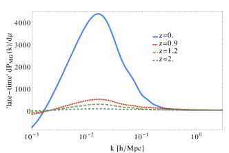
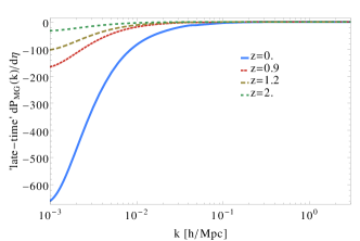
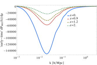
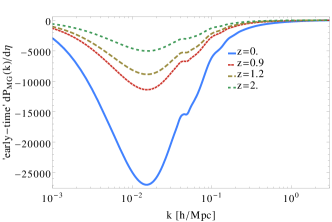
We can see from the previous figures that in the early-time parametrization the derivative of the power spectrum with respect to $\eta$ has a similar shape as the derivative with respect to $\mu$, making $\eta$ detectable by a Galaxy Clustering survey. To explain this, we derive the equation governing the evolution of density fluctuations for a cold dark matter (CDM) species, based on the equations implemented on the code MGCAMB presented in Hojjati et al. [2011], expressed here in the conformal Newtonian gauge. In the following, a dot represents derivative with respect to conformal time $\tau$:

$$\dot{\delta} =-(1+w)(\theta-3\dot{\Phi})-3\mathcal{H}(\frac{\delta P}{\delta\rho}-w)\delta$$ (55)

$$\dot{\theta} =-\mathcal{H}(1-3w)\theta-\frac{\dot{w}}{1+w}\theta+\frac{\delta P/\delta\rho}{1+w}k^{2}\delta-k^{2}\sigma+k^{2}\Psi$$ (56)

For CDM we have $\sigma=w=c^{2}_{s}=\delta P/\delta\rho=0$, then:

$$\dot{\delta} =-(\theta-3\dot{\Phi})$$ (57)

$$\dot{\theta} =-\mathcal{H}\theta+k^{2}\Psi$$ (58)

We have parameterized the solution to $\Psi$ as:

$$k^{2}\Psi=-4\pi Ga^{2}\mu(\tau)\rho(\tau)\delta(\tau)\quad,$$ (59)

and since we are also requiring gravitational slip $\eta=\Phi/\Psi$, we then have the Poisson equation for $\Phi$:

$$k^{2}\Phi=-4\pi Ga^{2}\mu(\tau)\eta(\tau)\rho(\tau)\delta(\tau)$$ (60)

Taking the time derivative of (57) and using (58) and (57) to replace $\dot{\theta}$ and $\theta$, and substituting $\Psi$ from (59), we obtain:

$$\ddot{\delta}+\mathcal{H}\dot{\delta} =3\mathcal{H}\dot{\Phi}+3\ddot{\Phi}+4\pi Ga^{2}\mu\rho\delta$$ (61)

In general, derivatives of $\Phi$ appearing on the right hand side will depend on both $\mu$ and $\eta$. Their contribution is larger in the early-time parameterization with respect to the late-time one.

Appendix C Other Decorrelation Methods

In section V.3 we have worked with a special decorrelation method, ZCA (Zero-phase component analysis, first introduced by Bell and Sejnowski [1997] in the context of image processing), which allows us to find a new vector of decorrelated variables $q$ that is as similar as possible to the original vector of variables $p$. Other decorrelation methods do not share this property, so in this section we want to illustrate their difference with respect to ZCA. In the next subsections we show for the Principal Component Analysis and Cholesky decomposition methods, a subset of our previous results, namely the Galaxy Clustering non-linear case, using the HS prescription for a Euclid survey with Redbook specifications.

C.0.1 Principal Component Analysis

Principal Component Analysis (PCA) Friedman [1987] is a well known method, which rotates the vector of variables $p$ into a new basis, using the eigenmatrix of the covariance matrix $C$. At the same time, it is the method that maximizes the compression of all components of $p$ into the components of $q$ using as measure the cross-covariance between $q$ and $p$ (see Kessy et al. [2015] for more details and references). This method is useful for dimensional reduction or data compression, since the information is stored in as few components as possible. This is achieved by using the $W$ matrix

$$W=\Lambda^{-1/2}U^{T}$$ (62)

where $\Lambda$ and $U$ represent the eigensystem of $C$ (defined in Eqn. 33).

Then, it follows that the transformed covariance matrix $\tilde{C}$ is whitened:

$$\tilde{C} =\Lambda^{-1/2}U^{T}C\Lambda^{-1/2}U^{T}$$ (63)

$$=\Lambda^{-1/2}U^{T}U\Lambda U^{T}\Lambda^{-1/2}U^{T}$$ (64)

$$=\mathbb{1}$$ (65)

As done previously, we renormalize $W$ in such a way that the sum of the square of the elements of each row sum up to unity. In Figure 23 we show in the left panel the weight matrix $W$ and in the right panel the 1$\sigma$ errors for the original and decorrelated variables. We see that the most constrained $q$ variables are the last components $q_{8}$-$q_{11}$, where most of the information has been compressed into. These 4 variables are complicated linear combinations of $A_{s}$, $\mu_{1,2,3}$ and $\eta_{1,2,3}$. This is the same we found for ZCA (cf. Fig. 8 and Eqns. (8)). However, the interpretation in terms of the old variables $p$ is not so simple anymore. We can see from the weight matrix and the 1$\sigma$ errors, that the most unconstrained parameter is $q_{1}$, which is basically equivalent to $\eta_{5}$. This means that this parameter can be eliminated from the analysis if one wants to do dimensional reduction.

Figure 23: Left: weight matrix $W$ for PCA. Right: 1$\sigma$ fully maximized errors on the primary parameters $p$ (blue lines) and the errors on the uncorrelated derived parameters $q$ (orange lines). Notice how all the important information is constrained in as few variables as possible, namely the last elements of $q_{i}$.

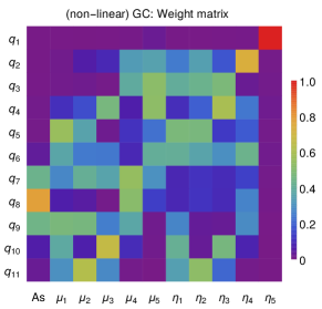
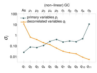
C.0.2 Cholesky decomposition

Cholesky decomposition of the Fisher matrix $F=LL^{T}$, allows us to define a decorrelation method that compresses all components of $p$ into an upper triangular matrix of components of $q$. This is achieved by using the $W$ matrix:

$$W=L^{T}$$ (66)

Then the covariance matrix will be whitened:

$$\tilde{C} =L^{T}(LL^{T})^{-1}L$$ (67)

$$=L^{T}(L^{T})^{-1}L^{-1}L$$ (68)

$$=\mathbb{1}$$ (69)

As done previously, we renormalize $W$ in such a way that the sum of the square of the elements of each row sum up to unity. In Cholesky decomposition, since we are constructing it via an upper triangular matrix (see left panel of Fig. 24), the new parameter $q_{11}$ will be identical to the parameter $\eta_{5}$, which is, as we have seen before (section V.4.1), the less constrained parameter. This decorrelation method is useful if one wants to have an ordering of the variables (see Kessy et al. [2015] and references therein). On the other hand $q_{1}$ is almost identical to $A_{s}$, since as we have seen in section V.4.1, it becomes decorrelated from the MG parameters in the non-linear case.

Figure 24: Left: weight matrix $W$ for the Cholesky decorrelation. Right: 1$\sigma$ fully maximized errors on the primary parameters $p$ (blue lines) and the errors on the uncorrelated derived parameters $q$ (orange lines). Notice how in this case, because of the upper triangular construction, the new variables $q_{9,10,11}$ are equivalent to $\eta_{3,4,5}$. The parameter $A_{s}$ is decorrelated in the non-linear HS case for GC, therefore it is almost equivalent to $q_{1}$ as was also the case in ZCA (compare with Fig. 6)

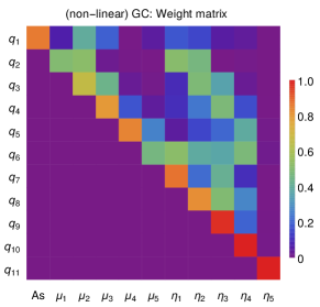
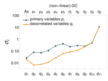
Appendix D Weight matrices coefficients

Here we explicitly show the coefficient of the $W$ matrices illustrated in Figures 6, 9 and 12. Tables 11 and 12 contain the coefficient matrices obtained for Galaxy Clustering in the linear and non-linear HS prescription cases respectively, while Tables 13 and 14 contain the coefficients obtained for WL. Finally, Table 15 reports the coefficients for the combination of GC, WL and Planck priors, in the non-linear HS case.

$$q_{i}=\footnotesize\left(\begin{array}[]{rrrrrrrrrrr}\color[rgb]{1,0,0}\definecolor[named]{pgfstrokecolor}{rgb}{1,0,0}0.899&0.003&-0.020&0.109&\color[rgb]{1,0,0}\definecolor[named]{pgfstrokecolor}{rgb}{1,0,0}0.315&0.250&0.097&0.021&-0.083&-0.022&-0.007\\ 0.001&\color[rgb]{1,0,0}\definecolor[named]{pgfstrokecolor}{rgb}{1,0,0}0.695&\color[rgb]{1,0,0}\definecolor[named]{pgfstrokecolor}{rgb}{1,0,0}-0.304&-0.089&-0.084&-0.026&\color[rgb]{1,0,0}\definecolor[named]{pgfstrokecolor}{rgb}{1,0,0}0.519&\color[rgb]{1,0,0}\definecolor[named]{pgfstrokecolor}{rgb}{1,0,0}-0.362&-0.082&-0.033&0.001\\ -0.003&-0.186&\color[rgb]{1,0,0}\definecolor[named]{pgfstrokecolor}{rgb}{1,0,0}0.745&-0.211&-0.090&-0.027&\color[rgb]{1,0,0}\definecolor[named]{pgfstrokecolor}{rgb}{1,0,0}-0.285&\color[rgb]{1,0,0}\definecolor[named]{pgfstrokecolor}{rgb}{1,0,0}0.491&-0.181&-0.036&0.001\\ 0.022&-0.065&\color[rgb]{1,0,0}\definecolor[named]{pgfstrokecolor}{rgb}{1,0,0}-0.252&\color[rgb]{1,0,0}\definecolor[named]{pgfstrokecolor}{rgb}{1,0,0}0.737&-0.174&-0.019&-0.075&\color[rgb]{1,0,0}\definecolor[named]{pgfstrokecolor}{rgb}{1,0,0}-0.320&\color[rgb]{1,0,0}\definecolor[named]{pgfstrokecolor}{rgb}{1,0,0}0.486&-0.116&0.001\\ 0.148&-0.142&-0.250&\color[rgb]{1,0,0}\definecolor[named]{pgfstrokecolor}{rgb}{1,0,0}-0.405&\color[rgb]{1,0,0}\definecolor[named]{pgfstrokecolor}{rgb}{1,0,0}0.666&0.070&-0.094&-0.102&\color[rgb]{1,0,0}\definecolor[named]{pgfstrokecolor}{rgb}{1,0,0}-0.268&\color[rgb]{1,0,0}\definecolor[named]{pgfstrokecolor}{rgb}{1,0,0}0.439&-0.002\\ \color[rgb]{1,0,0}\definecolor[named]{pgfstrokecolor}{rgb}{1,0,0}0.654&-0.246&\color[rgb]{1,0,0}\definecolor[named]{pgfstrokecolor}{rgb}{1,0,0}-0.420&-0.240&\color[rgb]{1,0,0}\definecolor[named]{pgfstrokecolor}{rgb}{1,0,0}0.388&\color[rgb]{1,0,0}\definecolor[named]{pgfstrokecolor}{rgb}{1,0,0}0.290&0.098&0.086&-0.159&0.003&-0.008\\ 0.026&\color[rgb]{1,0,0}\definecolor[named]{pgfstrokecolor}{rgb}{1,0,0}0.494&\color[rgb]{1,0,0}\definecolor[named]{pgfstrokecolor}{rgb}{1,0,0}-0.444&-0.098&-0.053&0.010&\color[rgb]{1,0,0}\definecolor[named]{pgfstrokecolor}{rgb}{1,0,0}0.621&\color[rgb]{1,0,0}\definecolor[named]{pgfstrokecolor}{rgb}{1,0,0}-0.375&-0.129&-0.055&-0.000\\ 0.004&\color[rgb]{1,0,0}\definecolor[named]{pgfstrokecolor}{rgb}{1,0,0}-0.265&\color[rgb]{1,0,0}\definecolor[named]{pgfstrokecolor}{rgb}{1,0,0}0.588&\color[rgb]{1,0,0}\definecolor[named]{pgfstrokecolor}{rgb}{1,0,0}-0.320&-0.044&0.007&\color[rgb]{1,0,0}\definecolor[named]{pgfstrokecolor}{rgb}{1,0,0}-0.288&\color[rgb]{1,0,0}\definecolor[named]{pgfstrokecolor}{rgb}{1,0,0}0.578&-0.248&-0.045&-0.000\\ -0.023&-0.082&\color[rgb]{1,0,0}\definecolor[named]{pgfstrokecolor}{rgb}{1,0,0}-0.295&\color[rgb]{1,0,0}\definecolor[named]{pgfstrokecolor}{rgb}{1,0,0}0.664&-0.158&-0.017&-0.135&\color[rgb]{1,0,0}\definecolor[named]{pgfstrokecolor}{rgb}{1,0,0}-0.338&\color[rgb]{1,0,0}\definecolor[named]{pgfstrokecolor}{rgb}{1,0,0}0.545&-0.102&0.001\\ -0.015&-0.082&-0.147&\color[rgb]{1,0,0}\definecolor[named]{pgfstrokecolor}{rgb}{1,0,0}-0.399&\color[rgb]{1,0,0}\definecolor[named]{pgfstrokecolor}{rgb}{1,0,0}0.651&0.001&-0.146&-0.155&\color[rgb]{1,0,0}\definecolor[named]{pgfstrokecolor}{rgb}{1,0,0}-0.257&\color[rgb]{1,0,0}\definecolor[named]{pgfstrokecolor}{rgb}{1,0,0}0.525&-0.000\\ \color[rgb]{1,0,0}\definecolor[named]{pgfstrokecolor}{rgb}{1,0,0}-0.519&\color[rgb]{1,0,0}\definecolor[named]{pgfstrokecolor}{rgb}{1,0,0}0.308&\color[rgb]{1,0,0}\definecolor[named]{pgfstrokecolor}{rgb}{1,0,0}0.510&\color[rgb]{1,0,0}\definecolor[named]{pgfstrokecolor}{rgb}{1,0,0}0.346&\color[rgb]{1,0,0}\definecolor[named]{pgfstrokecolor}{rgb}{1,0,0}-0.348&-0.239&-0.061&-0.070&0.181&-0.004&0.193\\ \end{array}\right)\cdot\footnotesize\begin{pmatrix}\ln(10^{10}A_{s})\\ \mu_{1}\\ \mu_{2}\\ \mu_{3}\\ \mu_{4}\\ \mu_{5}\\ \eta_{1}\\ \eta_{2}\\ \eta_{3}\\ \eta_{4}\\ \eta_{5}\end{pmatrix}$$

Table 11: Coefficients of the Matrix $W$ for the Euclid Redbook GC forecasted covariance matrix, using linear power spectra. The entries marked with red are those whose absolute values are larger than $0.25$.

$$q_{i}=\footnotesize\left(\begin{array}[]{rrrrrrrrrrr}\color[rgb]{1,0,0}\definecolor[named]{pgfstrokecolor}{rgb}{1,0,0}0.986&-0.064&-0.112&-0.093&-0.037&-0.038&-0.002&0.005&-0.002&0.005&0.002\\ -0.021&\color[rgb]{1,0,0}\definecolor[named]{pgfstrokecolor}{rgb}{1,0,0}0.677&\color[rgb]{1,0,0}\definecolor[named]{pgfstrokecolor}{rgb}{1,0,0}-0.349&-0.091&-0.042&-0.008&\color[rgb]{1,0,0}\definecolor[named]{pgfstrokecolor}{rgb}{1,0,0}0.516&\color[rgb]{1,0,0}\definecolor[named]{pgfstrokecolor}{rgb}{1,0,0}-0.367&-0.086&-0.021&0.001\\ -0.025&-0.233&\color[rgb]{1,0,0}\definecolor[named]{pgfstrokecolor}{rgb}{1,0,0}0.731&-0.194&-0.051&-0.011&\color[rgb]{1,0,0}\definecolor[named]{pgfstrokecolor}{rgb}{1,0,0}-0.317&\color[rgb]{1,0,0}\definecolor[named]{pgfstrokecolor}{rgb}{1,0,0}0.492&-0.166&-0.021&0.001\\ -0.030&-0.088&\color[rgb]{1,0,0}\definecolor[named]{pgfstrokecolor}{rgb}{1,0,0}-0.281&\color[rgb]{1,0,0}\definecolor[named]{pgfstrokecolor}{rgb}{1,0,0}0.755&-0.061&0.036&-0.073&\color[rgb]{1,0,0}\definecolor[named]{pgfstrokecolor}{rgb}{1,0,0}-0.331&\color[rgb]{1,0,0}\definecolor[named]{pgfstrokecolor}{rgb}{1,0,0}0.465&-0.086&-0.001\\ -0.032&-0.108&-0.197&-0.161&\color[rgb]{1,0,0}\definecolor[named]{pgfstrokecolor}{rgb}{1,0,0}0.820&0.238&-0.023&-0.092&-0.240&\color[rgb]{1,0,0}\definecolor[named]{pgfstrokecolor}{rgb}{1,0,0}0.357&-0.007\\ -0.086&-0.058&-0.110&\color[rgb]{1,0,0}\definecolor[named]{pgfstrokecolor}{rgb}{1,0,0}0.252&\color[rgb]{1,0,0}\definecolor[named]{pgfstrokecolor}{rgb}{1,0,0}0.637&\color[rgb]{1,0,0}\definecolor[named]{pgfstrokecolor}{rgb}{1,0,0}0.659&0.224&-0.001&-0.143&-0.046&-0.018\\ -0.001&\color[rgb]{1,0,0}\definecolor[named]{pgfstrokecolor}{rgb}{1,0,0}0.492&\color[rgb]{1,0,0}\definecolor[named]{pgfstrokecolor}{rgb}{1,0,0}-0.452&-0.071&-0.008&0.031&\color[rgb]{1,0,0}\definecolor[named]{pgfstrokecolor}{rgb}{1,0,0}0.617&\color[rgb]{1,0,0}\definecolor[named]{pgfstrokecolor}{rgb}{1,0,0}-0.391&-0.113&-0.038&-0.001\\ 0.001&\color[rgb]{1,0,0}\definecolor[named]{pgfstrokecolor}{rgb}{1,0,0}-0.296&\color[rgb]{1,0,0}\definecolor[named]{pgfstrokecolor}{rgb}{1,0,0}0.593&\color[rgb]{1,0,0}\definecolor[named]{pgfstrokecolor}{rgb}{1,0,0}-0.275&-0.029&-0.000&\color[rgb]{1,0,0}\definecolor[named]{pgfstrokecolor}{rgb}{1,0,0}-0.331&\color[rgb]{1,0,0}\definecolor[named]{pgfstrokecolor}{rgb}{1,0,0}0.575&-0.209&-0.031&-0.000\\ -0.001&-0.115&\color[rgb]{1,0,0}\definecolor[named]{pgfstrokecolor}{rgb}{1,0,0}-0.329&\color[rgb]{1,0,0}\definecolor[named]{pgfstrokecolor}{rgb}{1,0,0}0.635&-0.124&-0.028&-0.157&\color[rgb]{1,0,0}\definecolor[named]{pgfstrokecolor}{rgb}{1,0,0}-0.344&\color[rgb]{1,0,0}\definecolor[named]{pgfstrokecolor}{rgb}{1,0,0}0.558&-0.065&0.001\\ 0.008&-0.092&-0.136&\color[rgb]{1,0,0}\definecolor[named]{pgfstrokecolor}{rgb}{1,0,0}-0.390&\color[rgb]{1,0,0}\definecolor[named]{pgfstrokecolor}{rgb}{1,0,0}0.614&-0.030&-0.176&-0.167&-0.216&\color[rgb]{1,0,0}\definecolor[named]{pgfstrokecolor}{rgb}{1,0,0}0.581&0.001\\ 0.140&0.126&0.180&-0.194&\color[rgb]{1,0,0}\definecolor[named]{pgfstrokecolor}{rgb}{1,0,0}-0.645&\color[rgb]{1,0,0}\definecolor[named]{pgfstrokecolor}{rgb}{1,0,0}-0.608&-0.218&-0.029&0.137&0.049&0.199\\ \end{array}\right)\cdot\footnotesize\begin{pmatrix}\ln(10^{10}A_{s})\\ \mu_{1}\\ \mu_{2}\\ \mu_{3}\\ \mu_{4}\\ \mu_{5}\\ \eta_{1}\\ \eta_{2}\\ \eta_{3}\\ \eta_{4}\\ \eta_{5}\end{pmatrix}$$

Table 12: Coefficients of the Matrix $W$ for the Euclid Redbook GC forecasted covariance matrix, using the non-linear HS prescription. The entries marked with red are those whose absolute values are larger than $0.25$.

$$q_{i}=\footnotesize\left(\begin{array}[]{rrrrrrrrrrr}\color[rgb]{1,0,0}\definecolor[named]{pgfstrokecolor}{rgb}{1,0,0}0.760&-0.005&\color[rgb]{1,0,0}\definecolor[named]{pgfstrokecolor}{rgb}{1,0,0}0.475&0.131&0.005&0.034&0.247&\color[rgb]{1,0,0}\definecolor[named]{pgfstrokecolor}{rgb}{1,0,0}0.329&0.095&0.004&-0.000\\ -0.000&\color[rgb]{1,0,0}\definecolor[named]{pgfstrokecolor}{rgb}{1,0,0}0.673&\color[rgb]{1,0,0}\definecolor[named]{pgfstrokecolor}{rgb}{1,0,0}-0.592&-0.055&0.013&0.008&\color[rgb]{1,0,0}\definecolor[named]{pgfstrokecolor}{rgb}{1,0,0}0.328&\color[rgb]{1,0,0}\definecolor[named]{pgfstrokecolor}{rgb}{1,0,0}-0.290&-0.034&-0.001&-0.000\\ 0.033&\color[rgb]{1,0,0}\definecolor[named]{pgfstrokecolor}{rgb}{1,0,0}-0.594&\color[rgb]{1,0,0}\definecolor[named]{pgfstrokecolor}{rgb}{1,0,0}0.674&0.013&-0.003&-0.000&\color[rgb]{1,0,0}\definecolor[named]{pgfstrokecolor}{rgb}{1,0,0}-0.302&\color[rgb]{1,0,0}\definecolor[named]{pgfstrokecolor}{rgb}{1,0,0}0.318&0.010&0.000&0.000\\ 0.075&\color[rgb]{1,0,0}\definecolor[named]{pgfstrokecolor}{rgb}{1,0,0}-0.457&0.112&\color[rgb]{1,0,0}\definecolor[named]{pgfstrokecolor}{rgb}{1,0,0}0.754&0.002&0.004&\color[rgb]{1,0,0}\definecolor[named]{pgfstrokecolor}{rgb}{1,0,0}-0.310&0.039&\color[rgb]{1,0,0}\definecolor[named]{pgfstrokecolor}{rgb}{1,0,0}0.326&0.001&0.000\\ 0.022&\color[rgb]{1,0,0}\definecolor[named]{pgfstrokecolor}{rgb}{1,0,0}0.892&-0.187&0.017&0.102&0.064&\color[rgb]{1,0,0}\definecolor[named]{pgfstrokecolor}{rgb}{1,0,0}0.326&-0.208&-0.064&-0.000&0.000\\ \color[rgb]{1,0,0}\definecolor[named]{pgfstrokecolor}{rgb}{1,0,0}0.251&\color[rgb]{1,0,0}\definecolor[named]{pgfstrokecolor}{rgb}{1,0,0}0.859&-0.030&0.048&0.098&0.090&\color[rgb]{1,0,0}\definecolor[named]{pgfstrokecolor}{rgb}{1,0,0}0.414&-0.078&-0.029&0.004&0.009\\ 0.034&\color[rgb]{1,0,0}\definecolor[named]{pgfstrokecolor}{rgb}{1,0,0}0.654&\color[rgb]{1,0,0}\definecolor[named]{pgfstrokecolor}{rgb}{1,0,0}-0.600&-0.074&0.009&0.008&\color[rgb]{1,0,0}\definecolor[named]{pgfstrokecolor}{rgb}{1,0,0}0.356&\color[rgb]{1,0,0}\definecolor[named]{pgfstrokecolor}{rgb}{1,0,0}-0.280&-0.037&-0.000&0.000\\ 0.047&\color[rgb]{1,0,0}\definecolor[named]{pgfstrokecolor}{rgb}{1,0,0}-0.606&\color[rgb]{1,0,0}\definecolor[named]{pgfstrokecolor}{rgb}{1,0,0}0.662&0.010&-0.006&-0.002&\color[rgb]{1,0,0}\definecolor[named]{pgfstrokecolor}{rgb}{1,0,0}-0.293&\color[rgb]{1,0,0}\definecolor[named]{pgfstrokecolor}{rgb}{1,0,0}0.324&0.013&0.001&0.001\\ 0.108&\color[rgb]{1,0,0}\definecolor[named]{pgfstrokecolor}{rgb}{1,0,0}-0.576&0.167&\color[rgb]{1,0,0}\definecolor[named]{pgfstrokecolor}{rgb}{1,0,0}0.655&-0.015&-0.005&\color[rgb]{1,0,0}\definecolor[named]{pgfstrokecolor}{rgb}{1,0,0}-0.311&0.105&\color[rgb]{1,0,0}\definecolor[named]{pgfstrokecolor}{rgb}{1,0,0}0.304&0.003&0.002\\ \color[rgb]{1,0,0}\definecolor[named]{pgfstrokecolor}{rgb}{1,0,0}0.256&\color[rgb]{1,0,0}\definecolor[named]{pgfstrokecolor}{rgb}{1,0,0}-0.718&\color[rgb]{1,0,0}\definecolor[named]{pgfstrokecolor}{rgb}{1,0,0}0.380&0.136&-0.003&0.032&-0.010&\color[rgb]{1,0,0}\definecolor[named]{pgfstrokecolor}{rgb}{1,0,0}0.448&0.197&0.111&0.061\\ -0.029&\color[rgb]{1,0,0}\definecolor[named]{pgfstrokecolor}{rgb}{1,0,0}-0.734&\color[rgb]{1,0,0}\definecolor[named]{pgfstrokecolor}{rgb}{1,0,0}0.253&0.068&0.000&0.166&0.084&\color[rgb]{1,0,0}\definecolor[named]{pgfstrokecolor}{rgb}{1,0,0}0.506&0.218&0.122&0.197\\ \end{array}\right)\cdot\footnotesize\begin{pmatrix}\ln(10^{10}A_{s})\\ \mu_{1}\\ \mu_{2}\\ \mu_{3}\\ \mu_{4}\\ \mu_{5}\\ \eta_{1}\\ \eta_{2}\\ \eta_{3}\\ \eta_{4}\\ \eta_{5}\end{pmatrix}$$

Table 13: Coefficients of the Matrix $W$ for the Euclid Redbook WL forecasted covariance matrix, using linear power spectra. The entries marked with red are those whose absolute values are larger than $0.25$.

$$q_{i}=\left(\footnotesize\begin{array}[]{rrrrrrrrrrr}\color[rgb]{1,0,0}\definecolor[named]{pgfstrokecolor}{rgb}{1,0,0}0.926&-0.004&\color[rgb]{1,0,0}\definecolor[named]{pgfstrokecolor}{rgb}{1,0,0}-0.323&-0.039&-0.040&-0.066&-0.043&-0.168&-0.004&-0.000&0.001\\ -0.000&\color[rgb]{1,0,0}\definecolor[named]{pgfstrokecolor}{rgb}{1,0,0}0.669&\color[rgb]{1,0,0}\definecolor[named]{pgfstrokecolor}{rgb}{1,0,0}-0.595&-0.051&0.012&0.013&\color[rgb]{1,0,0}\definecolor[named]{pgfstrokecolor}{rgb}{1,0,0}0.332&\color[rgb]{1,0,0}\definecolor[named]{pgfstrokecolor}{rgb}{1,0,0}-0.291&-0.031&-0.001&-0.000\\ -0.021&\color[rgb]{1,0,0}\definecolor[named]{pgfstrokecolor}{rgb}{1,0,0}-0.552&\color[rgb]{1,0,0}\definecolor[named]{pgfstrokecolor}{rgb}{1,0,0}0.711&0.029&0.005&0.016&\color[rgb]{1,0,0}\definecolor[named]{pgfstrokecolor}{rgb}{1,0,0}-0.270&\color[rgb]{1,0,0}\definecolor[named]{pgfstrokecolor}{rgb}{1,0,0}0.339&0.014&0.001&0.000\\ -0.025&\color[rgb]{1,0,0}\definecolor[named]{pgfstrokecolor}{rgb}{1,0,0}-0.460&\color[rgb]{1,0,0}\definecolor[named]{pgfstrokecolor}{rgb}{1,0,0}0.288&\color[rgb]{1,0,0}\definecolor[named]{pgfstrokecolor}{rgb}{1,0,0}0.725&0.016&0.040&-0.238&0.150&\color[rgb]{1,0,0}\definecolor[named]{pgfstrokecolor}{rgb}{1,0,0}0.312&0.002&0.000\\ -0.159&\color[rgb]{1,0,0}\definecolor[named]{pgfstrokecolor}{rgb}{1,0,0}0.657&\color[rgb]{1,0,0}\definecolor[named]{pgfstrokecolor}{rgb}{1,0,0}0.289&0.102&\color[rgb]{1,0,0}\definecolor[named]{pgfstrokecolor}{rgb}{1,0,0}0.476&0.156&\color[rgb]{1,0,0}\definecolor[named]{pgfstrokecolor}{rgb}{1,0,0}0.418&0.155&-0.007&0.006&0.001\\ -0.168&\color[rgb]{1,0,0}\definecolor[named]{pgfstrokecolor}{rgb}{1,0,0}0.455&\color[rgb]{1,0,0}\definecolor[named]{pgfstrokecolor}{rgb}{1,0,0}0.622&0.158&0.100&\color[rgb]{1,0,0}\definecolor[named]{pgfstrokecolor}{rgb}{1,0,0}0.486&0.223&0.236&-0.016&-0.001&-0.002\\ -0.006&\color[rgb]{1,0,0}\definecolor[named]{pgfstrokecolor}{rgb}{1,0,0}0.667&\color[rgb]{1,0,0}\definecolor[named]{pgfstrokecolor}{rgb}{1,0,0}-0.585&-0.053&0.015&0.012&\color[rgb]{1,0,0}\definecolor[named]{pgfstrokecolor}{rgb}{1,0,0}0.366&\color[rgb]{1,0,0}\definecolor[named]{pgfstrokecolor}{rgb}{1,0,0}-0.274&-0.026&0.000&-0.000\\ -0.023&\color[rgb]{1,0,0}\definecolor[named]{pgfstrokecolor}{rgb}{1,0,0}-0.560&\color[rgb]{1,0,0}\definecolor[named]{pgfstrokecolor}{rgb}{1,0,0}0.704&0.032&0.005&0.013&\color[rgb]{1,0,0}\definecolor[named]{pgfstrokecolor}{rgb}{1,0,0}-0.263&\color[rgb]{1,0,0}\definecolor[named]{pgfstrokecolor}{rgb}{1,0,0}0.345&0.017&0.001&0.000\\ -0.005&\color[rgb]{1,0,0}\definecolor[named]{pgfstrokecolor}{rgb}{1,0,0}-0.576&\color[rgb]{1,0,0}\definecolor[named]{pgfstrokecolor}{rgb}{1,0,0}0.277&\color[rgb]{1,0,0}\definecolor[named]{pgfstrokecolor}{rgb}{1,0,0}0.636&-0.002&-0.008&-0.238&0.165&\color[rgb]{1,0,0}\definecolor[named]{pgfstrokecolor}{rgb}{1,0,0}0.319&0.004&0.001\\ -0.026&\color[rgb]{1,0,0}\definecolor[named]{pgfstrokecolor}{rgb}{1,0,0}-0.506&\color[rgb]{1,0,0}\definecolor[named]{pgfstrokecolor}{rgb}{1,0,0}0.670&0.239&0.110&-0.037&0.114&\color[rgb]{1,0,0}\definecolor[named]{pgfstrokecolor}{rgb}{1,0,0}0.359&0.209&0.169&0.096\\ 0.180&\color[rgb]{1,0,0}\definecolor[named]{pgfstrokecolor}{rgb}{1,0,0}-0.799&0.053&0.033&0.069&-0.140&-0.055&0.044&0.134&\color[rgb]{1,0,0}\definecolor[named]{pgfstrokecolor}{rgb}{1,0,0}0.271&\color[rgb]{1,0,0}\definecolor[named]{pgfstrokecolor}{rgb}{1,0,0}0.452\\ \end{array}\right)\cdot\footnotesize\begin{pmatrix}\ln(10^{10}A_{s})\\ \mu_{1}\\ \mu_{2}\\ \mu_{3}\\ \mu_{4}\\ \mu_{5}\\ \eta_{1}\\ \eta_{2}\\ \eta_{3}\\ \eta_{4}\\ \eta_{5}\end{pmatrix}$$

Table 14: Coefficients of the Matrix $W$ for the Euclid Redbook WL forecasted covariance matrix, using the non-linear HS prescription. The entries marked with red are those whose absolute values are larger than $0.25$.

$$q_{i}=\left(\footnotesize\begin{array}[]{rrrrrrrrrrr}\color[rgb]{1,0,0}\definecolor[named]{pgfstrokecolor}{rgb}{1,0,0}0.932&0.033&0.149&0.220&0.202&0.138&-0.005&-0.026&-0.001&0.010&-0.003\\ 0.029&\color[rgb]{1,0,0}\definecolor[named]{pgfstrokecolor}{rgb}{1,0,0}0.839&-0.214&-0.085&-0.035&-0.021&\color[rgb]{1,0,0}\definecolor[named]{pgfstrokecolor}{rgb}{1,0,0}0.476&-0.119&-0.021&0.002&-0.000\\ 0.138&-0.222&\color[rgb]{1,0,0}\definecolor[named]{pgfstrokecolor}{rgb}{1,0,0}0.800&-0.083&0.016&0.028&\color[rgb]{1,0,0}\definecolor[named]{pgfstrokecolor}{rgb}{1,0,0}-0.256&\color[rgb]{1,0,0}\definecolor[named]{pgfstrokecolor}{rgb}{1,0,0}0.452&-0.118&-0.011&-0.002\\ \color[rgb]{1,0,0}\definecolor[named]{pgfstrokecolor}{rgb}{1,0,0}0.284&-0.123&-0.115&\color[rgb]{1,0,0}\definecolor[named]{pgfstrokecolor}{rgb}{1,0,0}0.791&0.076&0.108&-0.106&\color[rgb]{1,0,0}\definecolor[named]{pgfstrokecolor}{rgb}{1,0,0}-0.286&\color[rgb]{1,0,0}\definecolor[named]{pgfstrokecolor}{rgb}{1,0,0}0.387&-0.067&-0.010\\ \color[rgb]{1,0,0}\definecolor[named]{pgfstrokecolor}{rgb}{1,0,0}0.506&-0.097&0.043&0.148&\color[rgb]{1,0,0}\definecolor[named]{pgfstrokecolor}{rgb}{1,0,0}0.753&0.248&-0.059&-0.089&-0.144&0.222&-0.032\\ \color[rgb]{1,0,0}\definecolor[named]{pgfstrokecolor}{rgb}{1,0,0}0.545&-0.092&0.120&\color[rgb]{1,0,0}\definecolor[named]{pgfstrokecolor}{rgb}{1,0,0}0.331&\color[rgb]{1,0,0}\definecolor[named]{pgfstrokecolor}{rgb}{1,0,0}0.390&\color[rgb]{1,0,0}\definecolor[named]{pgfstrokecolor}{rgb}{1,0,0}0.626&-0.027&-0.088&-0.089&-0.009&0.104\\ -0.006&\color[rgb]{1,0,0}\definecolor[named]{pgfstrokecolor}{rgb}{1,0,0}0.621&\color[rgb]{1,0,0}\definecolor[named]{pgfstrokecolor}{rgb}{1,0,0}-0.322&-0.096&-0.028&-0.008&\color[rgb]{1,0,0}\definecolor[named]{pgfstrokecolor}{rgb}{1,0,0}0.656&\color[rgb]{1,0,0}\definecolor[named]{pgfstrokecolor}{rgb}{1,0,0}-0.261&-0.048&-0.009&-0.001\\ -0.032&-0.166&\color[rgb]{1,0,0}\definecolor[named]{pgfstrokecolor}{rgb}{1,0,0}0.605&\color[rgb]{1,0,0}\definecolor[named]{pgfstrokecolor}{rgb}{1,0,0}-0.276&-0.044&-0.028&\color[rgb]{1,0,0}\definecolor[named]{pgfstrokecolor}{rgb}{1,0,0}-0.277&\color[rgb]{1,0,0}\definecolor[named]{pgfstrokecolor}{rgb}{1,0,0}0.654&-0.148&-0.006&0.000\\ -0.003&-0.049&\color[rgb]{1,0,0}\definecolor[named]{pgfstrokecolor}{rgb}{1,0,0}-0.270&\color[rgb]{1,0,0}\definecolor[named]{pgfstrokecolor}{rgb}{1,0,0}0.634&-0.122&-0.048&-0.088&\color[rgb]{1,0,0}\definecolor[named]{pgfstrokecolor}{rgb}{1,0,0}-0.252&\color[rgb]{1,0,0}\definecolor[named]{pgfstrokecolor}{rgb}{1,0,0}0.659&-0.023&0.010\\ 0.067&0.015&-0.082&\color[rgb]{1,0,0}\definecolor[named]{pgfstrokecolor}{rgb}{1,0,0}-0.358&\color[rgb]{1,0,0}\definecolor[named]{pgfstrokecolor}{rgb}{1,0,0}0.614&-0.017&-0.055&-0.034&-0.074&\color[rgb]{1,0,0}\definecolor[named]{pgfstrokecolor}{rgb}{1,0,0}0.688&0.027\\ -0.072&-0.002&-0.060&-0.179&\color[rgb]{1,0,0}\definecolor[named]{pgfstrokecolor}{rgb}{1,0,0}-0.286&\color[rgb]{1,0,0}\definecolor[named]{pgfstrokecolor}{rgb}{1,0,0}0.591&-0.027&0.008&0.108&0.088&\color[rgb]{1,0,0}\definecolor[named]{pgfstrokecolor}{rgb}{1,0,0}0.713\\ \end{array}\right)\cdot\footnotesize\begin{pmatrix}\ln(10^{10}A_{s})\\ \mu_{1}\\ \mu_{2}\\ \mu_{3}\\ \mu_{4}\\ \mu_{5}\\ \eta_{1}\\ \eta_{2}\\ \eta_{3}\\ \eta_{4}\\ \eta_{5}\end{pmatrix}$$

Table 15: Coefficients of the Matrix $W$ for the Euclid Redbook GC+WL case using the non-linear HS prescription and adding a CMB Planck prior. The entries marked with red are those whose absolute values are larger than $0.25$.

Appendix E The Kullback-Leibler divergence

In Section IV.4 we exploited the determinant of the covariance matrix $C$ as a Figure of Merit for our forecasts. Here we summarize a possible alternative, the Kullback-Leibler divergence Kullback and Leibler [1951], also called relative entropy or information gain. It has been used in the field of cosmology for model selection, experiment design and forecasting, see among others Kunz et al. [2006], Raveri et al. [2016], Seehars et al. [2014], Verde et al. [2013], Zhao et al. [2017]. The KL-divergence $\mathcal{D}(p_{2}||p_{1})$ measures for a continuous, $d$-dimensional random variable $\theta$, the relative entropy between two probability density functions $p_{1}(\theta)$ and $p_{2}(\theta)$ and it is given by

$$\mathcal{D}(p_{2}||p_{1})\equiv\int p_{2}(\theta)\ln\left(\frac{p_{2}(\theta)}{p_{1}(\theta)}\right)\mathrm{d}\theta.$$ (70)

Although it is not symmetric in $p_{1}$ and $p_{2}$ it can be interpreted as a distance between the two distributions and measures the information gain since it is non-negative ($\mathcal{D}(p_{2}||p_{1})\geq 0$), non-degenerate ($\mathcal{D}(p_{2}||p_{1})=0$ if and only if $p_{1}=p_{2}$) and it is invariant under re-parametrizations of the distributions as $p_{1}(\theta)\mathrm{d}\theta=p_{1}(\tilde{\theta})\mathrm{d}\tilde{\theta}$. In the form given here the information gain is measured in nits as in section IV.4, to convert nits to bits it is enough to divide the result by $\ln(2)$.

For the special case of $p_{1}(\theta)$ and $p_{2}(\theta)$ being multivariate Gaussian distributions, with the same mean values and covariance matrices $\mathcal{A}$ and $\mathcal{B}$ respectively, we obtain

$$\mathcal{D}(p_{2}||p_{1})=-\frac{1}{2}\left[\ln\left(\frac{\det(\mathcal{A})}{\det(\mathcal{B})}\right)+\mathrm{Tr}\left[\mathbb{1}-\mathcal{B}^{-1}\mathcal{A}\right]\right].$$ (71)

We then define a Kullback-Leibler matrix $\mathcal{K}$ composed of the KL-divergence measure among our observables, defined as:

$$\mathcal{K}_{ij}=\mathcal{D}(p_{j}||p_{i}).$$ (72)

where $p_{i}$ and $p_{j}$ represent our observables: GC(lin), GC(nl-HS), WL(lin), WL(nl-HS), GC+WL(lin) and GC+WL(nl-HS) in the redshift binned parameterization of section V. In this way we can quantitatively see how much information is gained when going from one probe like Galaxy Clustering to another probe like Weak Lensing. In Figure 25 we plot in the left panel the KL matrix $\mathcal{K}_{ij}$ when no Planck priors are added and in the right panel the KL matrix when Planck priors are added to all probes. For visualization purposes, we plot the logarithm of the KL matrix: $\log_{10}\mathcal{K}_{ij}$. Blue (red) colours represent small (large) information gain, while black represents no information gain at all, which is by construction the case on the diagonal, $\mathcal{K}_{ii}=0$. The rows of the matrix represent the reference observable of $p_{1}$ and the columns, the new observable $p_{2}$. The information gain when going from a linear WL observable to a non-linear GC observable or to a combined GC+WL (linear and non-linear) observable is considerably high at about $\approx 10^{6}$-$10^{7}$. However, when adding a Planck prior, this gets reduced by at least 2 orders of magnitude, since the prior is strong and then there is not as much new information gained in the new observables. On the opposite case, we can see that the row corresponding to GC+WL(nl-HS) is mostly blue, meaning that there is little gain of information when going to one of the other observables.

Figure 25: Kullback-Leibler divergence matrices $\mathcal{K}_{ij}$. This matrix represents graphically the information gain between all possible observables in the redshift binned parameterization of section V. We have plotted here the logarithm of the KL-divergence matrix, for illustrative purposes. Therefore the diagonal is $-\infty$ and it is represented by a black color. Left: KL matrix without Planck priors. The maximum gain is about $10^{7}$ when going from WL(lin) to GC+WL(non-linear) and we can observe that GC+WL does not gain extra information when complemented with the other observables, which is expected. Right: In this case we compare the observables, when a Planck prior is added beforehand. The overall information gain is now smaller, with a maximum of about $10^{6}$. The maximum gain comes when comparing WL (linear and non-linear) to GC and GC+WL (non-linear).

References

- Planck Collaboration et al. [2016] Planck Collaboration, P. A. R. Ade, and others. Planck 2015 results. XIV. Dark energy and modified gravity. Astronomy and Astrophysics, 594:A14, September 2016. doi: 10.1051/0004-6361/201525814. URL http://arxiv.org/abs/1502.01590.
- Amendola and others [2013] Luca Amendola and others. Cosmology and fundamental physics with the Euclid satellite. Living Reviews in Relativity, 16, 2013. ISSN 1433-8351. doi: 10.12942/lrr-2013-6. URL http://arxiv.org/abs/1206.1225.
- Casas et al. [2015] Santiago Casas, Luca Amendola, Marco Baldi, Valeria Pettorino, and Adrian Vollmer. Fitting and forecasting non-linear coupled dark energy. arXiv:1508.07208 [astro-ph], August 2015. URL http://arxiv.org/abs/1508.07208.
- Bielefeld et al. [2014] Jannis Bielefeld, Dragan Huterer, and Eric V. Linder. Cosmological Leverage from the Matter Power Spectrum in the Presence of Baryon and Nonlinear Effects. SciRate, November 2014. URL https://scirate.com/arxiv/1411.3725.
- Kunz [2012] Martin Kunz. The phenomenological approach to modeling the dark energy. Comptes Rendus Physique, 13(6-7):539–565, July 2012. ISSN 16310705. doi: 10.1016/j.crhy.2012.04.007. URL http://arxiv.org/abs/1204.5482.
- Amendola et al. [2013] Luca Amendola, Martin Kunz, Mariele Motta, Ippocratis D. Saltas, and Ignacy Sawicki. Observables and unobservables in dark energy cosmologies. Physical Review D, 87:023501, January 2013. ISSN 0556-2821. doi: 10.1103/PhysRevD.87.023501. URL http://arxiv.org/abs/1210.0439.
- Alonso et al. [2016] David Alonso, Emilio Bellini, Pedro G. Ferreira, and Miguel Zumalacarregui. The Observational Future of Cosmological Scalar-Tensor Theories. arXiv:1610.09290 [astro-ph, physics:gr-qc, physics:hep-th], October 2016. URL http://arxiv.org/abs/1610.09290. arXiv: 1610.09290.
- Hojjati et al. [2012] Alireza Hojjati, Gong-Bo Zhao, Levon Pogosian, Alessandra Silvestri, Robert Crittenden, and Kazuya Koyama. Cosmological tests of General Relativity: a principal component analysis. Phys. Rev., D85:043508, 2012. doi: 10.1103/PhysRevD.85.043508. URL https://arxiv.org/abs/1111.3960.
- Baker and Bull [2015] Tessa Baker and Philip Bull. Observational signatures of modified gravity on ultra-large scales. The Astrophysical Journal, 811(2):116, September 2015. ISSN 1538-4357. doi: 10.1088/0004-637X/811/2/116. URL http://arxiv.org/abs/1506.00641.
- Bull [2015] Philip Bull. Extending cosmological tests of General Relativity with the Square Kilometre Array. arXiv:1509.07562 [astro-ph, physics:gr-qc], September 2015. URL http://arxiv.org/abs/1509.07562.
- Gleyzes et al. [2016] Jérôme Gleyzes, David Langlois, Michele Mancarella, and Filippo Vernizzi. Effective Theory of Dark Energy at Redshift Survey Scales. Journal of Cosmology and Astroparticle Physics, 2016(02):056–056, February 2016. ISSN 1475-7516. doi: 10.1088/1475-7516/2016/02/056. URL http://arxiv.org/abs/1509.02191. arXiv: 1509.02191.
- Hojjati et al. [2011] Alireza Hojjati, Levon Pogosian, and Gong-Bo Zhao. Testing gravity with CAMB and CosmoMC. JCAP, 1108:005, 2011. doi: 10.1088/1475-7516/2011/08/005.
- Smith et al. [2003] R. E. Smith, J. A. Peacock, A. Jenkins, S. D. M. White, C. S. Frenk, F. R. Pearce, P. A. Thomas, G. Efstathiou, and H. M. P. Couchman. Stable clustering, the halo model and non-linear cosmological power spectra. MNRAS, 341(4):1311–1332, June 2003. ISSN 0035-8711, 1365-2966. doi: 10.1046/j.1365-8711.2003.06503.x. URL http://mnras.oxfordjournals.org/content/341/4/1311.
- Takahashi et al. [2012] Ryuichi Takahashi, Masanori Sato, Takahiro Nishimichi, Atsushi Taruya, and Masamune Oguri. Revising the Halofit Model for the Nonlinear Matter Power Spectrum. arXiv:1208.2701, August 2012. URL http://arxiv.org/abs/1208.2701.
- Hu and Sawicki [2007] Wayne Hu and Ignacy Sawicki. A Parameterized Post-Friedmann Framework for Modified Gravity. Phys.Rev., D76:104043, 2007. doi: 10.1103/PhysRevD.76.104043.
- Saltas et al. [2014] Ippocratis D. Saltas, Ignacy Sawicki, Luca Amendola, and Martin Kunz. Anisotropic Stress as a Signature of Nonstandard Propagation of Gravitational Waves. Phys. Rev. Lett., 113(19):191101, 2014. doi: 10.1103/PhysRevLett.113.191101.
- Sawicki et al. [2016] Ignacy Sawicki, Ippocratis D. Saltas, Mariele Motta, Luca Amendola, and Martin Kunz. Non-standard gravitational waves imply gravitational slip: on the difficulty of partially hiding new gravitational degrees of freedom. 2016.
- Pogosian et al. [2010] L. Pogosian, A. Silvestri, K. Koyama, and G.-B. Zhao. How to optimally parametrize deviations from general relativity in the evolution of cosmological perturbations. Phys. Rev., D81(10):104023, May 2010. doi: 10.1103/PhysRevD.81.104023.
- Gubitosi et al. [2013] Giulia Gubitosi, Federico Piazza, and Filippo Vernizzi. The Effective Field Theory of Dark Energy. Journal of Cosmology and Astroparticle Physics, 2013(02):032–032, February 2013. ISSN 1475-7516. doi: 10.1088/1475-7516/2013/02/032. URL http://arxiv.org/abs/1210.0201. arXiv: 1210.0201.
- Bellini et al. [2016] Emilio Bellini, Antonio J. Cuesta, Raul Jimenez, and Licia Verde. Constraints on deviations from ${\Lambda}$CDM within Horndeski gravity. Journal of Cosmology and Astroparticle Physics, 2016(02):053–053, February 2016. ISSN 1475-7516. doi: 10.1088/1475-7516/2016/02/053. URL http://arxiv.org/abs/1509.07816. arXiv: 1509.07816.
- Bellini and Sawicki [2014] Emilio Bellini and Ignacy Sawicki. Maximal freedom at minimum cost: linear large-scale structure in general modifications of gravity. arXiv:1404.3713 [astro-ph, physics:gr-qc], April 2014. URL http://arxiv.org/abs/1404.3713. arXiv: 1404.3713.
- Zhao et al. [2009] Gong-Bo Zhao, Levon Pogosian, Alessandra Silvestri, and Joel Zylberberg. Searching for modified growth patterns with tomographic surveys. Phys. Rev., D79:083513, 2009. doi: 10.1103/PhysRevD.79.083513.
- Lewis et al. [2000] Antony Lewis, Anthony Challinor, and Anthony Lasenby. Efficient Computation of CMB anisotropies in closed FRW models. Astrophys. J., 538:473–476, 2000. doi: 10.1086/309179.
- Bernardeau et al. [2001] F. Bernardeau, S. Colombi, E. Gaztanaga, and R. Scoccimarro. Large-Scale Structure of the Universe and Cosmological Perturbation Theory. arXiv:astro-ph/0112551, December 2001. doi: 10.1016/S0370-1573(02)00135-7. URL http://arxiv.org/abs/astro-ph/0112551.
- Bernardeau [2013] Francis Bernardeau. The evolution of the large-scale structure of the universe: beyond the linear regime. arXiv:1311.2724 [astro-ph], November 2013. URL http://arxiv.org/abs/1311.2724.
- Crocce and Scoccimarro [2006] Martín Crocce and Román Scoccimarro. Renormalized cosmological perturbation theory. Physical Review D, 73(6):063519, March 2006. doi: 10.1103/PhysRevD.73.063519. URL http://link.aps.org/doi/10.1103/PhysRevD.73.063519.
- Blas et al. [2016] Diego Blas, Mathias Garny, Mikhail M. Ivanov, and Sergey Sibiryakov. Time-sliced perturbation theory II: baryon acoustic oscillations and infrared resummation. Journal of Cosmology and Astroparticle Physics, 2016(07):028, 2016. ISSN 1475-7516. doi: 10.1088/1475-7516/2016/07/028. URL http://stacks.iop.org/1475-7516/2016/i=07/a=028.
- Taruya and Hiramatsu [2008] Atsushi Taruya and Takashi Hiramatsu. A Closure Theory for Non-linear Evolution of Cosmological Power Spectra. The Astrophysical Journal, 674(2):617–635, February 2008. ISSN 0004-637X, 1538-4357. doi: 10.1086/526515. URL http://arxiv.org/abs/0708.1367.
- Pietroni [2008] Massimo Pietroni. Flowing with Time: a New Approach to Nonlinear Cosmological Perturbations. JCAP, 0810:036, 2008. doi: 10.1088/1475-7516/2008/10/036.
- Anselmi and Pietroni [2012] Stefano Anselmi and Massimo Pietroni. Nonlinear power spectrum from resummed perturbation theory: a leap beyond the BAO scale. Journal of Cosmology and Astroparticle Physics, 2012(12):013, 2012. URL http://iopscience.iop.org/1475-7516/2012/12/013.
- Carrasco et al. [2012] John Joseph M. Carrasco, Mark P. Hertzberg, and Leonardo Senatore. The effective field theory of cosmological large scale structures. Journal of High Energy Physics, 2012(9):1–40, 2012. URL http://link.springer.com/article/10.1007/JHEP09(2012)082.
- Baumann et al. [2012] Daniel Baumann, Alberto Nicolis, Leonardo Senatore, and Matias Zaldarriaga. Cosmological non-linearities as an effective fluid. Journal of Cosmology and Astroparticle Physics, 2012(07):051, 2012. URL http://iopscience.iop.org/1475-7516/2012/07/051.
- Pietroni et al. [2011] Massimo Pietroni, Gianpiero Mangano, Ninetta Saviano, and Matteo Viel. Coarse-Grained Cosmological Perturbation Theory. arXiv:1108.5203 [astro-ph, physics:hep-th], August 2011. URL http://arxiv.org/abs/1108.5203.
- Manzotti et al. [2014] Alessandro Manzotti, Marco Peloso, Massimo Pietroni, Matteo Viel, and Francisco Villaescusa-Navarro. A coarse grained perturbation theory for the Large Scale Structure, with cosmology and time independence in the UV. arXiv:1407.1342 [astro-ph, physics:gr-qc, physics:hep-th], July 2014. URL http://arxiv.org/abs/1407.1342.
- Springel [2005] Volker Springel. The cosmological simulation code GADGET-2. Mon. Not. Roy. Astron. Soc., 364:1105–1134, 2005.
- Fosalba et al. [2013] P. Fosalba, M. Crocce, E. Gaztanaga, and F. J. Castander. The MICE Grand Challenge Lightcone Simulation I: Dark matter clustering. arXiv preprint arXiv:1312.1707, 2013. URL http://arxiv.org/abs/1312.1707.
- Lawrence et al. [2010] Earl Lawrence, Katrin Heitmann, Martin White, David Higdon, Christian Wagner, Salman Habib, and Brian Williams. The coyote universe. III. simulation suite and precision emulator for the nonlinear matter power spectrum. The Astrophysical Journal, 713(2):1322, 2010. URL http://iopscience.iop.org/0004-637X/713/2/1322.
- Heitmann et al. [2014] Katrin Heitmann, Earl Lawrence, Juliana Kwan, Salman Habib, and David Higdon. The Coyote Universe Extended: Precision Emulation of the Matter Power Spectrum. The Astrophysical Journal, 780(1):111, 2014. URL http://iopscience.iop.org/0004-637X/780/1/111.
- Heymans and others [2013] Catherine Heymans and others. CFHTLenS tomographic weak lensing cosmological parameter constraints: Mitigating the impact of intrinsic galaxy alignments. Mon. Not. Roy. Astron. Soc., 432:2433, 2013. doi: 10.1093/mnras/stt601.
- Kitching and others [2014] T. D. Kitching and others. 3d Cosmic Shear: Cosmology from CFHTLenS. Mon. Not. Roy. Astron. Soc., 442(2):1326–1349, 2014. doi: 10.1093/mnras/stu934.
- Zhao [2014] Gong-Bo Zhao. Modeling the nonlinear clustering in modified gravity models I: A fitting formula for matter power spectrum of f(R) gravity. The Astrophysical Journal Supplement Series, 211(2):23, April 2014. ISSN 0067-0049, 1538-4365. doi: 10.1088/0067-0049/211/2/23. URL http://arxiv.org/abs/1312.1291.
- Taruya et al. [2014] Atsushi Taruya, Takahiro Nishimichi, Francis Bernardeau, Takashi Hiramatsu, and Kazuya Koyama. Regularized cosmological power spectrum and correlation function in modified gravity models. Physical Review D, 90(12), December 2014. ISSN 1550-7998, 1550-2368. doi: 10.1103/PhysRevD.90.123515. URL http://arxiv.org/abs/1408.4232.
- Saracco et al. [2010] F. Saracco, M. Pietroni, N. Tetradis, V. Pettorino, and G. Robbers. Non-linear Matter Spectra in Coupled Quintessence. Physical Review D, 82(2), July 2010. ISSN 1550-7998, 1550-2368. doi: 10.1103/PhysRevD.82.023528. URL http://arxiv.org/abs/0911.5396.
- Vollmer et al. [2014] Adrian Vollmer, Luca Amendola, and Riccardo Catena. Efficient implementation of the Time Renormalization Group. arXiv:1412.1650 [astro-ph, physics:physics], December 2014. URL http://arxiv.org/abs/1412.1650.
- Brouzakis et al. [2011] N. Brouzakis, V. Pettorino, N. Tetradis, and C. Wetterich. Nonlinear matter spectra in growing neutrino quintessence. JCAP, 1103:049, 2011. doi: 10.1088/1475-7516/2011/03/049.
- Bird et al. [2011] Simeon Bird, Matteo Viel, and Martin G. Haehnelt. Massive Neutrinos and the Non-linear Matter Power Spectrum. arXiv:1109.4416, September 2011. doi: 10.1111/j.1365-2966.2011.20222.x. URL http://arxiv.org/abs/1109.4416.
- Zhao et al. [2011] Gong-Bo Zhao, Baojiu Li, and Kazuya Koyama. N-body Simulations for f(R) Gravity using a Self-adaptive Particle-Mesh Code. Physical Review D, 83(4), February 2011. ISSN 1550-7998, 1550-2368. doi: 10.1103/PhysRevD.83.044007. URL http://arxiv.org/abs/1011.1257.
- Koyama et al. [2009] Kazuya Koyama, Atsushi Taruya, and Takashi Hiramatsu. Non-linear Evolution of Matter Power Spectrum in Modified Theory of Gravity. Physical Review D, 79(12), June 2009. ISSN 1550-7998, 1550-2368. doi: 10.1103/PhysRevD.79.123512. URL http://arxiv.org/abs/0902.0618.
- Tegmark et al. [1998] Max Tegmark, Andrew Hamilton, Michael Strauss, Michael Vogeley, and Alexander Szalay. Measuring the galaxy power spectrum with future redshift surveys. The Astrophysical Journal, 499(2):555–576, June 1998. ISSN 0004-637X, 1538-4357. doi: 10.1086/305663. URL http://arxiv.org/abs/astro-ph/9708020.
- Seo and Eisenstein [2007] Hee-Jong Seo and Daniel J. Eisenstein. Improved forecasts for the baryon acoustic oscillations and cosmological distance scale. The Astrophysical Journal, 665(1):14–24, August 2007. ISSN 0004-637X, 1538-4357. doi: 10.1086/519549. URL http://arxiv.org/abs/astro-ph/0701079.
- Seo and Eisenstein [2005] Hee-Jong Seo and Daniel J. Eisenstein. Baryonic acoustic oscillations in simulated galaxy redshift surveys. The Astrophysical Journal, 633(2):575–588, November 2005. ISSN 0004-637X, 1538-4357. doi: 10.1086/491599. URL http://arxiv.org/abs/astro-ph/0507338.
- Mukherjee et al. [2008] Pia Mukherjee, Martin Kunz, David Parkinson, and Yun Wang. Planck priors for dark energy surveys. Physical Review D, 78(8), October 2008. ISSN 1550-7998, 1550-2368. doi: 10.1103/PhysRevD.78.083529. URL http://arxiv.org/abs/0803.1616.
- Laureijs and others [2011] R. Laureijs and others. Euclid Definition Study Report. arXiv:1110.3193 [astro-ph], October 2011. URL http://arxiv.org/abs/1110.3193.
- Yahya et al. [2015] S. Yahya, P. Bull, M. G. Santos, M. Silva, R. Maartens, P. Okouma, and B. Bassett. Cosmological performance of SKA HI galaxy surveys. Monthly Notices of the Royal Astronomical Society, 450(3):2251–2260, May 2015. ISSN 0035-8711, 1365-2966. doi: 10.1093/mnras/stv695. URL http://arxiv.org/abs/1412.4700.
- Santos et al. [2015] Mario G. Santos, David Alonso, Philip Bull, Marta Silva, and Sahba Yahya. HI galaxy simulations for the SKA: number counts and bias. arXiv:1501.03990 [astro-ph], January 2015. URL http://arxiv.org/abs/1501.03990.
- Raccanelli et al. [2015] Alvise Raccanelli, Philip Bull, Stefano Camera, David Bacon, Chris Blake, Olivier Dore, Pedro Ferreira, Roy Maartens, Mario Santos, Matteo Viel, and Gong-bo Zhao. Measuring redshift-space distortions with future SKA surveys. 2015.
- Bull et al. [2015] Philip Bull, Stefano Camera, Alvise Raccanelli, Chris Blake, Pedro G. Ferreira, Mario G. Santos, and Dominik J. Schwarz. Measuring baryon acoustic oscillations with future SKA surveys. arXiv:1501.04088 [astro-ph], January 2015. URL http://arxiv.org/abs/1501.04088.
- Harrison et al. [2016] Ian Harrison, Stefano Camera, Joe Zuntz, and Michael L. Brown. SKA Weak Lensing I: Cosmological Forecasts and the Power of Radio-Optical Cross-Correlations. arXiv:1601.03947 [astro-ph], January 2016. URL http://arxiv.org/abs/1601.03947.
- DESI Collaboration et al. [2016a] DESI Collaboration, Amir Aghamousa, and others. The DESI Experiment Part I: Science,Targeting, and Survey Design. arXiv:1611.00036 [astro-ph], October 2016a. URL http://arxiv.org/abs/1611.00036.
- DESI Collaboration et al. [2016b] DESI Collaboration, Amir Aghamousa, and others. The DESI Experiment Part II: Instrument Design. arXiv:1611.00037 [astro-ph], October 2016b. URL http://arxiv.org/abs/1611.00037.
- Levi et al. [2013] Michael Levi, Chris Bebek, Timothy Beers, Robert Blum, Robert Cahn, Daniel Eisenstein, Brenna Flaugher, Klaus Honscheid, Richard Kron, Ofer Lahav, Patrick McDonald, Natalie Roe, David Schlegel, and representing the DESI collaboration. The DESI Experiment, a whitepaper for Snowmass 2013. arXiv:1308.0847 [astro-ph], August 2013. URL http://arxiv.org/abs/1308.0847.
- de la Torre and Guzzo [2012] Sylvain de la Torre and Luigi Guzzo. Modelling non-linear redshift-space distortions in the galaxy clustering pattern: systematic errors on the growth rate parameter. arXiv:1202.5559 [astro-ph], February 2012. URL http://arxiv.org/abs/1202.5559.
- Alcock and Paczynski [1979] C. Alcock and B. Paczynski. An evolution free test for non-zero cosmological constant. Nature, 281:358, October 1979. ISSN 0028-0836. doi: 10.1038/281358a0. URL http://adsabs.harvard.edu/abs/1979Natur.281..358A.
- Ballinger et al. [1996] W. E. Ballinger, J. A. Peacock, and A. F. Heavens. Measuring the cosmological constant with redshift surveys. Monthly Notices of the Royal Astronomical Society, 282:877, October 1996. ISSN 0035-8711. doi: 10.1093/mnras/282.3.877. URL http://adsabs.harvard.edu/abs/1996MNRAS.282..877B.
- Feldman et al. [1994] Hume A. Feldman, Nick Kaiser, and John A. Peacock. Power Spectrum Analysis of Three-Dimensional Redshift Surveys. The Astrophysical Journal, 426:23, May 1994. ISSN 0004-637X, 1538-4357. doi: 10.1086/174036. URL http://arxiv.org/abs/astro-ph/9304022.
- Amendola et al. [2012] Luca Amendola, Valeria Pettorino, Claudia Quercellini, and Adrian Vollmer. Testing coupled dark energy with next-generation large-scale observations. Physical Review D, 85(10), May 2012. ISSN 1550-7998, 1550-2368. doi: 10.1103/PhysRevD.85.103008. URL http://link.aps.org/doi/10.1103/PhysRevD.85.103008.
- Bailoni et al. [2016] Alberto Bailoni, Alessio Spurio Mancini, and Luca Amendola. Improving Fisher matrix forecasts for galaxy surveys: window function, bin cross-correlation, and bin redshift uncertainty. ArXiv e-prints, 1608:arXiv:1608.00458, August 2016. URL http://adsabs.harvard.edu/abs/2016arXiv160800458B.
- Lewis and Bridle [2002] Antony Lewis and Sarah Bridle. Cosmological parameters from CMB and other data: A Monte Carlo approach. Phys. Rev., D66:103511, 2002. doi: 10.1103/PhysRevD.66.103511.
- Lewis [2013] Antony Lewis. Efficient sampling of fast and slow cosmological parameters. Phys. Rev., D87(10):103529, 2013. doi: 10.1103/PhysRevD.87.103529.
- Hu and Sugiyama [1996] Wayne Hu and Naoshi Sugiyama. Small Scale Cosmological Perturbations: An Analytic Approach. The Astrophysical Journal, 471(2):542–570, November 1996. ISSN 0004-637X, 1538-4357. doi: 10.1086/177989. URL http://arxiv.org/abs/astro-ph/9510117.
- Simpson and Peacock [2010] Fergus Simpson and John A. Peacock. Difficulties Distinguishing Dark Energy from Modified Gravity via Redshift Distortions. Physical Review D, 81(4), February 2010. ISSN 1550-7998, 1550-2368. doi: 10.1103/PhysRevD.81.043512. URL http://arxiv.org/abs/0910.3834. arXiv: 0910.3834.
- Leonard et al. [2015] C. Danielle Leonard, Tessa Baker, and Pedro G. Ferreira. Exploring degeneracies in modified gravity with weak lensing. Physical Review D, 91(8), April 2015. ISSN 1550-7998, 1550-2368. doi: 10.1103/PhysRevD.91.083504. URL http://arxiv.org/abs/1501.03509. arXiv: 1501.03509.
- Bell and Sejnowski [1997] Anthony J. Bell and Terrence J. Sejnowski. The “independent components” of natural scenes are edge filters. Vision Research, 37(23):3327 – 3338, 1997. ISSN 0042-6989. doi: http://dx.doi.org/10.1016/S0042-6989(97)00121-1. URL http://www.sciencedirect.com/science/article/pii/S0042698997001211.
- Kessy et al. [2015] Agnan Kessy, Alex Lewin, and Korbinian Strimmer. Optimal whitening and decorrelation. arXiv:1512.00809 [stat], December 2015. URL http://arxiv.org/abs/1512.00809.
- Lacasa and Rosenfeld [2016] Fabien Lacasa and Rogerio Rosenfeld. Combining cluster number counts and galaxy clustering. JCAP, 1608:005, March 2016. doi: 10.1088/1475-7516/2016/08/005,10.1088/1475-7516/2016/08/005. URL https://arxiv.org/abs/1603.00918.
- Friedman [1987] Jerome H. Friedman. Exploratory projection pursuit. Journal of the American Statistical Association, 82(397):249–266, 1987. doi: 10.1080/01621459.1987.10478427. URL http://amstat.tandfonline.com/doi/abs/10.1080/01621459.1987.10478427.
- Kullback and Leibler [1951] S. Kullback and R. A. Leibler. On Information and Sufficiency. The Annals of Mathematical Statistics, 22(1):79–86, March 1951. ISSN 0003-4851, 2168-8990. doi: 10.1214/aoms/1177729694. URL http://projecteuclid.org/euclid.aoms/1177729694.
- Kunz et al. [2006] M. Kunz, N. Aghanim, L. Cayon, O. Forni, A. Riazuelo, and J. P. Uzan. Constraining topology in harmonic space. Physical Review D, 73(2), January 2006. ISSN 1550-7998, 1550-2368. doi: 10.1103/PhysRevD.73.023511. URL http://arxiv.org/abs/astro-ph/0510164.
- Raveri et al. [2016] Marco Raveri, Matteo Martinelli, Gongbo Zhao, and Yuting Wang. CosmicFish Implementation Notes V1.0. arXiv:1606.06268 [astro-ph, physics:gr-qc], June 2016. URL http://arxiv.org/abs/1606.06268.
- Seehars et al. [2014] Sebastian Seehars, Adam Amara, Alexandre Refregier, Aseem Paranjape, and Joël Akeret. Information Gains from Cosmic Microwave Background Experiments. Physical Review D, 90(2), July 2014. ISSN 1550-7998, 1550-2368. doi: 10.1103/PhysRevD.90.023533. URL http://arxiv.org/abs/1402.3593.
- Verde et al. [2013] Licia Verde, Pavlos Protopapas, and Raul Jimenez. Planck and the local Universe: Quantifying the tension. Physics of the Dark Universe, 2(3):166–175, September 2013. ISSN 2212-6864. doi: 10.1016/j.dark.2013.09.002. URL http://www.sciencedirect.com/science/article/pii/S2212686413000319.
- Zhao et al. [2017] Gong-Bo Zhao, Marco Raveri, Levon Pogosian, Yuting Wang, Robert G. Crittenden, Will J. Handley, Will J. Percival, Jonathan Brinkmann, Chia-Hsun Chuang, Antonio J. Cuesta, Daniel J. Eisenstein, Francisco-Shu Kitaura, Kazuya Koyama, Benjamin L’Huillier, Robert C. Nichol, Matthew M. Pieri, Sergio Rodriguez-Torres, Ashley J. Ross, Graziano Rossi, Ariel G. Sánchez, Arman Shafieloo, Jeremy L. Tinker, Rita Tojeiro, Jose A. Vazquez, and Hanyu Zhang. The clustering of galaxies in the completed SDSS-III Baryon Oscillation Spectroscopic Survey: Examining the observational evidence for dynamical dark energy. 2017.