Tree-level correlations in
the strong field regime

Abstract

We consider the correlation function of an arbitrary number of local observables in quantum field theory. We show that, at tree level in the strong field regime, these correlations arise solely from fluctuations in the initial state. We obtain the general expression of these correlation functions in terms of the classical solution of the field equation of motion and its derivatives with respect to its initial conditions, that can be arranged graphically as the sum of labeled trees where the nodes are the individual observables, and the links are pairs of derivatives acting on them. For $3$-point (and higher) correlation functions, there are additional tree-level terms beyond from the strong field approximation, generated throughout the evolution of the system.

1 Introduction

A common question in many areas is the evaluation of correlations between several measurements, given the microscopic dynamics of the system. This problem comes up for instance in the calculation of cosmological perturbations [1, 2], or in nuclear physics, e.g. in heavy ion collisions [3, 4]. These situations have in common that they are described by some underlying quantum field theory, and that the system starts from some supposedly known initial state. Then, it evolves under the effect of the self-interactions of the fields, and possibly the couplings to some external sources. Thereafter, we define an observable as some local operator ${\cal O}(\phi(x))$ constructed from the fields of the theory. Our goal in this paper is to study (at leading order in the couplings) the correlations between measurements of this observable at several space-time points $x_{1},x_{2},\cdots,x_{n}$,

$${\cal C}_{\{1\cdots n\}}\equiv\big{<}0{}_{\rm in}\big{|}{\cal O}(\phi(x_{1}))\cdots{\cal O}(\phi(x_{n}))\big{|}0{}_{\rm in}\big{>}_{\rm c}\;.$$ (1)

In this definition, we have assumed that the system is initially in the perturbative vacuum state (see the appendices B and C for a discussion of the changes with other types of initial states). The subscript “c” indicates the connected part of this expectation value, i.e. the terms that contain the actual correlations. An important restriction in our discussion will be to consider only points $x_{i}$ that all have space-like separations, i.e. $(x_{i}-x_{j})^{2}<0$. Physically, this means that the measurement performed at one of the points cannot influence the outcome of the measurement at another point. Therefore, the correlations between the measurements are entirely due to the past evolution of the system.

The main difference compared to the more familiar problem of computing cross-sections is that the final state is not prescribed. Instead, one wishes to calculate the expectation value of some operators, by summing over all the possible final states given a prescribed initial state. One could in principle perform such a calculation by using the usual techniques for calculating transition amplitudes, by first writing

$$\big{<}{\rm in}\big{|}{\cal O}\big{|}{\rm in}\big{>}=\sum_{{\rm f},{\rm f}^{\prime}}\big{<}{\rm in}\big{|}{\rm f}\big{>}\big{<}{\rm f}\big{|}{\cal O}\big{|}{\rm f}^{\prime}\big{>}\big{<}{\rm f}^{\prime}\big{|}{\rm in}\big{>}\;.$$ (2)

(The double sum over final states could be reduced to a single sum if we use eigenstates of the observable ${\cal O}$.) All the steps involved in this pedestrian approach can be encapsulated in a set of diagrammatic rules known as the Schwinger-Keldysh formalism, or in-in formalism [5, 6, 7, 8] (see also [9, 10]), that roughly consists in two copies of the usual Feynman rules (one that gives the factor $\big{<}{\rm f}^{\prime}\big{|}{\rm in}\big{>}$, and one –complex conjugated– that gives the factor $\big{<}{\rm in}\big{|}{\rm f}\big{>}$), plus some additional rules that give the final state sum. The approach we follow in this paper bears heavily on earlier works in the field of heavy ion collisions [11, 12, 13, 14] and in cosmology [2, 15].

Although the approach used in this paper and the final result are quite general, the intermediate derivations are a bit cumbersome. In order to keep the notations as light as possible, we consider a theory with a single real scalar field $\phi$, whose Lagrangian density is given by

$${\cal L}\equiv\frac{1}{2}(\partial_{\mu}\phi)(\partial^{\mu}\phi)-\frac{1}{2}m^{2}\,\phi^{2}\underbrace{-V(\phi)+J\phi}_{{\cal L}_{\rm int}(\phi)}\;,$$ (3)

where $V(\phi)$ contains the self-interactions of the field and $J(x)$ is an external source. The quantum field theory described by the Lagrangian density (3) has a well known perturbative expansion. However, we are interested in this paper in the strong field regime, where this perturbative expansion is insufficient. This corresponds to fields for which the interaction term $V(\phi)$ is as large as the kinetic term $(\partial_{\mu}\phi)(\partial^{\mu}\phi)$,

$$(\partial_{\mu}\phi)(\partial^{\mu}\phi)\sim V(\phi)\;,$$ (4)

implying that the interactions cannot be treated as a perturbation. For instance, for a theory with a quartic interaction term $V(\phi)\sim g^{2}\phi^{4}$, this occurs for fields

$$\phi\sim\frac{Q}{g}\;,$$ (5)

where $Q$ is some typical momentum scale in the problem (the field $\phi$ has the dimension of a momentum in four space-time dimensions). For fields driven by an external source, the term $J\phi$ must also have the same order of magnitude as the kinetic and self-interaction terms, and thus the order of magnitude of the source that may create this large field is

$$J\sim\frac{Q^{3}}{g}\;.$$ (6)

In order to see where the usual perturbative expansion fails, let us recall the power counting in the case of a theory with a $g^{2}\phi^{4}$ interaction term. The order of magnitude of a connected graph ${\cal G}$ with $n_{{}_{E}}$ external legs, $n_{{}_{L}}$ loops and $n_{{}_{J}}$ external sources is given by

$${\cal G}\sim g^{-2}g^{-n_{{}_{E}}}g^{-2n_{{}_{L}}}\big{(}gJ\big{)}^{n_{{}_{J}}}\;.$$ (7)

Eq. (6) implies that $gJ$ cannot be treated as a small expansion parameter. Any quantity must therefore be evaluated non-perturbatively in the number of sources $n_{{}_{J}}$. In contrast, the hierarchy of the contributions based on the number of loops in the Feynman diagrams survives. Our aim is to calculate the correlation function (1) to lowest order in the number of loops (i.e. at tree level) but to all order in $n_{{}_{J}}$ (or equivalently to all orders in the field amplitude).

With large fields, the correlation function (1) is suppressed compared to the uncorrelated part, because each propagator connecting a pair of observables costs a factor $g^{2}$ (the endpoints of such a link replace two fields of order $g^{-1}$). In order to fully connect the $n$ observables, $n-1$ propagators are necessary, suppressing the correlation by a factor $g^{2(n-1)}$ with respect to the uncorrelated part. Thus, in a certain sense, the correlation function may be viewed as a higher order correction. At leading order, $1$-point functions (i.e. the expectation value of a local observable) are obtained from a classical solution of the field equation of motion, obeying a retarded boundary condition that depends on the initial state ($\phi=\dot{\phi}=0$ when the initial state is the perturbative vacuum) [11]. Their next-to-leading order (NLO) corrections are also known [13], and can be expressed in terms of functional derivatives of this classical field with respect to its initial condition. A similar result was proven in [14] for the NLO correction to a $2$-point function, that contains its tree-level correlated part.

In this paper, we assess to what extent a similar representation exists for the correlated part of higher $n$-point functions at tree-level. We prove that, within the strong field approximation (defined in the section 5), the tree-level correlation between any number of arbitrary local observables takes the following graphical form:

$${\cal C}_{\{1\cdots n\}}=\sum_{{\mbox{\scriptsize trees with }n}\atop{\mbox{\scriptsize labeled nodes}}}\raise-48.36967pt\hbox to106.69783pt{\leavevmode\resizebox{106.69783pt}{}{\includegraphics{tree_example2}}}\;,$$ (8)

where the nodes are the observables evaluated for a classical solution of the field equation of motion, and the links are pairs of derivatives with respect to the initial condition of the classical field.

The paper is organized as follows. In the section 2, we couple the observable ${\cal O}(\phi(x))$ to a fictitious source $z({\boldsymbol{x}})$ in order to define a generating functional whose derivatives give the expectation for the combined measurement of ${\cal O}(\phi(x))$ at several points. We explain how to obtain this generating functional diagrammatically by extending the Schwinger-Keldysh formalism with an extra vertex that corresponds to the observable, and then we rephrase this diagrammatic expansion in the retarded-advanced basis, that will be useful to discuss the strong field regime. In the section 3, we study the first derivative of the generating functional. At leading order, it can be expressed in terms of a pair of fields that obey classical equations of motion and satisfy non-trivial $z$-dependent boundary conditions. In the following section 4, we set up an expansion of these fields order by order in powers of the function $z({\boldsymbol{x}})$, and we determine explicitly the first two orders, that give the $1$-point and $2$-point correlation functions. We also show how to rewrite the $2$-point function in terms of derivatives of a classical field with respect to its initial condition. In the section 5, we consider the strong field approximation, and we determine the solution to all orders in $z$ in this approximation. We show that the tree level $n$-point correlation function in this approximation can be represented as the sum of all trees with $n$ labeled nodes (the $n$ instances of the observable), and pairwise links that are differential operators with respect to the initial condition of the classical field. The section 6 illustrates on the example of the $3$-point function the type of contributions that arise at tree level beyond the strong field approximation. Summary and conclusions are in the section 7. In the appendix A, we derive some technical points used in the main part of the paper, while in the appendices B and C we discuss other types of initial states.

2 Generating functional for local measurements

2.1 Definition

For simplicity, we will take the points $x_{i}$ where the measurements are performed to lie on the same surface of constant time $x^{0}=t_{f}$, but the final results would be valid for any locally space-like surface (in order to ensure that there is no causal relation between the points $x_{i}$).

One can encapsulate all the correlation functions (1) into a generating functional defined as follows:

$${\cal F}[z({\boldsymbol{x}})]\equiv\big{<}0{}_{\rm in}\big{|}\exp\int_{t_{f}}{\rm d}^{3}{\boldsymbol{x}}\;z({\boldsymbol{x}})\,{\cal O}(\phi(x))\big{|}0{}_{\rm in}\big{>}\;,$$ (9)

where the argument of the field in ${\cal O}$ is $x\equiv(t_{f},{\boldsymbol{x}})$. From this generating functional, the correlation functions are obtained by differentiating with respect to $z({\boldsymbol{x}}_{1}),\cdots,z({\boldsymbol{x}}_{n})$ and by setting $z\equiv 0$ afterwards. In order to remove the uncorrelated part of the $n$-point function, we should differentiate the logarithm of ${\cal F}$, i.e.

$${\cal C}_{\{1\cdots n\}}=\left.\frac{\delta^{n}\ln{\cal F}}{\delta z({\boldsymbol{x}}_{1})\cdots\delta z({\boldsymbol{x}}_{n})}\right|_{z\equiv 0}$$ (10)

Note that since the final surface is space-like and the operators ${\cal O}(\phi(x))$ are local, there is no need for a specific ordering of the exponential. The observable ${\cal O}(\phi(x))$ is made of the field in the Heisenberg picture, $\phi(x)$, that can be related to the field $\phi_{\rm in}(x)$ of the interaction picture as follows:

$$\phi(x)=U(-\infty,x^{0})\,\phi_{\rm in}(x)\,U(x^{0},-\infty)\;,$$ (11)

where $U(t_{1},t_{2})$ is an evolution operator given in terms of the interactions by the following formula

$$U(t_{2},t_{1})={\rm T}\,\exp i\int_{t_{1}}^{t_{2}}{\rm d}x^{0}{\rm d}^{3}{\boldsymbol{x}}\;{\cal L}_{\rm int}(\phi_{\rm in}(x))\;.$$ (12)

We can therefore rewrite the generating functional solely in terms of the interaction picture field $\phi_{\rm in}$,

$${\cal F}[z({\boldsymbol{x}})] = \big{<}0{}_{\rm in}\big{|}{\rm P}\,\exp\int{\rm d}^{3}{\boldsymbol{x}}\;\Big{\{}i\int{\rm d}x^{0}\;{\cal L}_{\rm int}(\phi_{{\rm in}+}(x))-{\cal L}_{\rm int}(\phi_{{\rm in}-}(x))$$ (13)

$$\qquad\qquad\qquad\qquad\qquad+z({\boldsymbol{x}})\,{\cal O}(\phi_{\rm in}(t_{f},{\boldsymbol{x}}))\Big{\}}\big{|}0{}_{\rm in}\big{>}\;,$$

where ${\rm P}$ denotes a path ordering on the following time contour:

The operators are ordered from left to right starting from the end of the contour. We denote by $\phi_{{\rm in}+}$ the field that lives on the upper branch and by $\phi_{{\rm in}-}$ the field on the lower branch (the minus sign in front of the term ${\cal L}_{\rm int}(\phi_{{\rm in}-}(x))$ comes from the fact that the lower branch is oriented from $+\infty$ to $-\infty$). The operator ${\cal O}(\phi_{\rm in}(x))$ lives at the final time of this contour, and could either be viewed as made of fields of type $+$ or of type $-$ (the two choices lead to the same results). Note that in eq. (13), the spacetime integration is a priori extended to the domain located below the final surface (the observable ${\cal O}$ therefore lives on the upper time boundary of the integration domain). However, this restriction is not really necessary: by causality, the contribution of the domain located above $t_{f}$ would cancel anyhow.

2.2 Expression in the Schwinger-Keldysh formalism

Since the initial state is the vacuum, the generating functional defined in eq. (13) can be represented diagrammatically as the sum of all the vacuum-to-vacuum graphs (i.e. graphs without external legs) in the Schwinger-Keldysh formalism (also known as the in-in formalism), extended by an extra vertex that corresponds to the insertions of the observable ${\cal O}$. Let us recall here that the Schwinger-Keldysh diagrammatic rules consist in having two types of interaction vertices ($+$ and $-$ depending on which branch of the contour the vertex lies on, the $-$ vertex being the opposite of the $+$ one) and four types of bare propagators ($G_{++}^{0},G_{--}^{0},G_{+-}^{0}$ and $G_{-+}^{0}$) depending on the location of the endpoints on the contour. The additional vertex exists only on the final surface, at the time $t_{f}$. It is accompanied by a factor $z({\boldsymbol{x}})$, and has as many legs as there are fields in ${\cal O}$. There is only one kind of this vertex (we can decide to call it $+$ or $-$ without affecting anything). We recapitulate these Feynman rules in the figure 1.

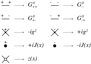
Figure 1: Diagrammatic rules for the extended Schwinger-Keldysh formalism that gives the generating functional. The Feynman rules shown here for the self-interactions correspond to a $g^{2}\phi^{4}/4!$ interaction term. In this illustration, we have assumed that the observable is quartic in the field when drawing the corresponding vertex (proportional to $z({\boldsymbol{x}})$).

In the case of the vacuum initial state, the propagators have the following explicit expressions:

$$G_{-+}^{0}(x,y)=\int_{\boldsymbol{k}}e^{-ik\cdot(x-y)}\;,\quad G_{+-}^{0}(x,y)=\int_{\boldsymbol{k}}e^{ik\cdot(x-y)}\;,$$

$$G_{++}^{0}(x,y)=\theta(x^{0}-y^{0})\,G_{-+}^{0}(x,y)+\theta(y^{0}-x^{0})\,G_{+-}^{0}(x,y)\;,$$

$$G_{--}^{0}(x,y)=\theta(x^{0}-y^{0})\,G_{+-}^{0}(x,y)+\theta(y^{0}-x^{0})\,G_{-+}^{0}(x,y)\;,$$ (14)

where we have used the following compact notation

$$\int_{\boldsymbol{k}}\cdots\equiv\int\frac{{\rm d}^{3}{\boldsymbol{k}}}{(2\pi)^{3}2E_{\boldsymbol{k}}}\cdots\qquad(E_{\boldsymbol{k}}\equiv\sqrt{{\boldsymbol{k}}^{2}+m^{2}})\;.$$ (15)

Note that when we set $z\equiv 0$, these diagrammatic rules fall back to the pure Schwinger-Keldysh formalism, for which it is known that all the connected vacuum-to-vacuum graphs are zero. This implies that

$${\cal F}[z\equiv 0]=1\;,$$ (16)

in accordance with the fact that this should be $\big{<}0{}_{\rm in}\big{|}0{}_{\rm in}\big{>}=1$.

2.3 Retarded-advanced representation

In order to clarify what approximations may be done in the large field regime, it is useful to use a different basis of fields by introducing [16, 17]

$$\phi_{2}\equiv\tfrac{1}{2}\,\big{(}\phi_{+}+\phi_{-}\big{)}\;,\qquad\phi_{1}\equiv\phi_{+}-\phi_{-}\;.$$ (17)

The half-sum $\phi_{2}$ in a sense captures the classical content (plus some quantum corrections), while the difference $\phi_{1}$ is purely quantum (because it represents the different histories of the fields in the amplitude and in the complex conjugated amplitude). To see how the Feynman rules are modified in terms of these new fields, let us start from

$$\phi_{\alpha}=\sum_{\epsilon=\pm}\Omega_{\alpha\epsilon}\,\phi_{\epsilon}\qquad(\alpha=1,2)\;,$$ (18)

where the matrix $\Omega$ reads:

$$\Omega_{\alpha\epsilon}\equiv\begin{pmatrix}1&-1\\ 1/2&1/2\\ \end{pmatrix}\;.$$ (19)

In terms of this matrix, the new propagators are obtained as follows

$${G}_{\alpha\beta}^{0}\equiv\sum_{\epsilon,\epsilon^{\prime}=\pm}\Omega_{\alpha\epsilon}\Omega_{\beta\epsilon^{\prime}}{G}_{\epsilon\epsilon^{\prime}}^{0}\;.$$ (20)

Explicitly, these propagators read

$$G_{21}^{0} = G_{++}^{0}-G_{+-}^{0}\;,$$

$$G_{12}^{0} = G_{++}^{0}-G_{-+}^{0}\;,$$

$$G_{22}^{0} = \tfrac{1}{2}\,\left[G_{+-}^{0}+G_{-+}^{0}\right]\;,$$

$$G_{11}^{0} = 0\;.$$ (21)

Note that $G_{21}^{0}$ is the bare retarded propagator, while $G_{12}^{0}$ is the bare advanced propagator. The vertices in the new formalism (here written for a quartic interaction) are given by

$$\Gamma_{\alpha\beta\gamma\delta}\equiv-ig^{2}\left[\Omega^{-1}_{+\alpha}\Omega^{-1}_{+\beta}\Omega^{-1}_{+\gamma}\Omega^{-1}_{+\delta}-\Omega^{-1}_{-\alpha}\Omega^{-1}_{-\beta}\Omega^{-1}_{-\gamma}\Omega^{-1}_{-\delta}\right]\;,$$ (22)

where

$$\Omega^{-1}_{\epsilon\alpha}=\begin{pmatrix}1/2&1\\ -1/2&1\\ \end{pmatrix}\qquad\qquad[\Omega_{\alpha\epsilon}\Omega_{\epsilon\beta}^{-1}=\delta_{\alpha\beta}]\;.$$ (23)

More explicitly, we have :

$$\Gamma_{1111}=\Gamma_{1122}=\Gamma_{2222}=0$$

$$\Gamma_{1222}=-ig^{2}\;,\quad\Gamma_{1112}=-ig^{2}/4\;.$$ (24)

(The vertices not listed explicitly here are obtained by permutations.) Finally, the rules for an external source in the retarded-advanced basis are :

$$J_{1}=J\;,\quad J_{2}=0\;.$$ (25)

Finally, note that the observable depends only on the field $\phi_{2}$, i.e. ${\cal O}={\cal O}(\phi_{2})$. Indeed, the fields $\phi_{+}$ and $\phi_{-}$ represent the field in the amplitude and in the conjugated amplitude. Their difference should vanish when a measurement is performed.

3 First derivative at tree level

3.1 First derivative of $\ln{\cal F}$

Differentiating the generating functional with respect to $z({\boldsymbol{x}})$ amounts to exhibiting a vertex ${\cal O}$ at the point ${\boldsymbol{x}}$ at the final time (as opposed to weighting this vertex by $z({\boldsymbol{x}})$ and integrating over ${\boldsymbol{x}}$). Furthermore, by considering the logarithm of the generating functional rather than ${\cal F}$ itself, we have only diagrams that are connected to the point ${\boldsymbol{x}}$, as shown in this representation:

$$\frac{\delta\ln{\cal F}}{\delta z({\boldsymbol{x}})}=\;\raise-18.20973pt\hbox to71.13188pt{\leavevmode\resizebox{71.13188pt}{}{\includegraphics{1der}}}\;\;,$$ (26)

where the gray blob is a sum of graphs constructed with the Feynman rules of the figure 1, or their analogue in the retarded-advanced formulation. Therefore, these graphs still depend implicitly on $z$. Note that this blob does not have to be connected.

3.2 Tree level expression

Without further specifying the content of the blob, eq. (26) is valid to all orders, both in $z$ and in $g$. At lowest order in $g$ (tree level), a considerable simplification happens because the blob must be a product of disconnected subgraphs, one for each line attached to the vertex ${\cal O}(\phi(x))$:

$$\left.\frac{\delta\ln{\cal F}}{\delta z({\boldsymbol{x}})}\right|_{\rm tree}=\;\raise-20.20146pt\hbox to56.9055pt{\leavevmode\resizebox{56.9055pt}{}{\includegraphics{1der-tree}}}\;\;,$$ (27)

where now each of the light colored blob is a connected tree $1$-point diagram. In the retarded-advanced formalism, there are two of these $1$-point functions, that we will denote $\phi_{1}$ and $\phi_{2}$. At tree level, they can be defined recursively by the following pair of coupled integral equations:

$$\phi_{1}(x) = i\int_{\Omega}{\rm d}^{4}y\;G_{12}^{0}(x,y)\,\frac{\partial{\boldsymbol{L}}_{\rm int}(\phi_{1},\phi_{2})}{\partial\phi_{2}(y)}$$

$$\qquad+\int_{t_{f}}{\rm d}^{3}{\boldsymbol{y}}\;G_{12}^{0}(x,y)\;z({\boldsymbol{y}})\;{\cal O}^{\prime}(\phi_{2}(y))\;,$$

$$\phi_{2}(x) = i\int_{\Omega}{\rm d}^{4}y\;\Big{\{}G_{21}^{0}(x,y)\,\frac{\partial{\boldsymbol{L}}_{\rm int}(\phi_{1},\phi_{2})}{\partial\phi_{1}(y)}+G_{22}^{0}(x,y)\,\frac{\partial{\boldsymbol{L}}_{\rm int}(\phi_{1},\phi_{2})}{\partial\phi_{2}(y)}\Big{\}}$$ (28)

$$\qquad+\int_{t_{f}}{\rm d}^{3}{\boldsymbol{y}}\;G_{22}^{0}(x,y)\;z({\boldsymbol{y}})\;{\cal O}^{\prime}(\phi_{2}(y))\;.$$

In these equations, ${\cal O}^{\prime}$ is the derivative of the observable with respect to the field, $\Omega$ is the space-time domain comprised between the initial and final times, and we denote

$${\boldsymbol{L}}_{\rm int}(\phi_{1},\phi_{2})\equiv{\cal L}_{\rm int}(\phi_{2}+\tfrac{1}{2}\phi_{1})-{\cal L}_{\rm int}(\phi_{2}-\tfrac{1}{2}\phi_{1})\;.$$ (29)

For an interaction Lagrangian $-\tfrac{g^{2}}{4!}\phi^{4}+J\phi$, this difference reads

$${\boldsymbol{L}}_{\rm int}(\phi_{1},\phi_{2})=-\frac{g^{2}}{6}\phi_{2}^{3}\phi_{1}-\frac{g^{2}}{4!}\phi_{1}^{3}\phi_{2}+J\phi_{1}\;.$$ (30)

In terms of these fields, we have

$$\left.\frac{\delta\ln{\cal F}}{\delta z({\boldsymbol{x}})}\right|_{\rm tree}={\cal O}(\phi_{2}(x))\;,$$ (31)

i.e. simply the observable ${\cal O}$ evaluated on the field $\phi_{2}(x)$ (but this field depends on $z$ to all orders, via the boundary terms in eqs. (28)).

3.3 Classical equations of motion

Using the fact that $G_{12}^{0}$ and $G_{21}^{0}$ are Green’s functions of $\square+m^{2}$, respectively obeying the following identities

$$(\square_{x}+m^{2})\,G_{12}^{0}(x,y)=-i\delta(x-y)\;,\quad(\square_{x}+m^{2})\,G_{21}^{0}(x,y)=+i\delta(x-y)\;,$$ (32)

while $G_{22}^{0}$ vanishes when acted upon by this operator,

$$(\square_{x}+m^{2})\,G_{22}^{0}(x,y)=0\;,$$ (33)

we see that $\phi_{1}$ and $\phi_{2}$ obey the following classical field equations of motion:

$$(\square_{x}+m^{2})\,\phi_{1}(x)=\frac{\partial{\boldsymbol{L}}_{\rm int}(\phi_{1},\phi_{2})}{\partial\phi_{2}(x)}\;,$$

$$(\square_{x}+m^{2})\,\phi_{2}(x)=\frac{\partial{\boldsymbol{L}}_{\rm int}(\phi_{1},\phi_{2})}{\partial\phi_{1}(x)}\;.$$ (34)

Note that here the point $x$ is located in the “bulk” $\Omega$; this is why the observable does not enter in these equations of motion. In fact, the observable enters only in the boundary conditions satisfied by these fields on the hypersurface at $t_{f}$. For later reference, let us also rewrite these equations of motion in the specific case of a scalar field theory with a $g^{2}\phi^{4}/4!$ interaction term and an external source $J$:

$$\Big{[}\square_{x}+m^{2}+\tfrac{g^{2}}{2}\phi_{2}^{2}\Big{]}\,\phi_{1}+\frac{g^{2}}{4!}\,\phi_{1}^{3}=0\;,$$

$$(\square_{x}+m^{2})\,\phi_{2}+\frac{g^{2}}{6}\,\phi_{2}^{3}+\frac{g^{2}}{8}\,\phi_{1}^{2}\phi_{2}=J\;.$$ (35)

3.4 Boundary conditions

The equations of motion (34) are easier to handle than the integral equations (28), but they must be supplemented with boundary conditions in order to define uniquely the solutions. The standard procedure for deriving the boundary conditions is to consider the combination $G_{12}^{0}(x,y)\,({\square}_{y}+m^{2})\,\phi_{1}(y)$, and let the operator $\square_{y}+m^{2}$ act alternatively on the right and on the left,

$$G_{12}^{0}(x,y)\,(\stackrel{{\scriptstyle\rightarrow}}{{\square}}_{y}+m^{2})\,\phi_{1}(y)=G_{12}^{0}(x,y)\,\frac{\partial{\boldsymbol{L}}_{\rm int}(\phi_{1},\phi_{2})}{\partial\phi_{2}(y)}$$

$$G_{12}^{0}(x,y)\,(\stackrel{{\scriptstyle\leftarrow}}{{\square}}_{y}+m^{2})\,\phi_{1}(y)=-i\delta(x-y)\,\phi_{1}(y)\;.$$ (36)

By subtracting these equations and integrating over $y\in\Omega$, we obtain

$$\phi_{1}(x)=i\int_{\Omega}{\rm d}^{4}y\;G_{12}^{0}(x,y)\,\frac{\partial{\boldsymbol{L}}_{\rm int}(\phi_{1},\phi_{2})}{\partial\phi_{2}(y)}-i\int_{\Omega}{\rm d}^{4}y\;G_{12}^{0}(x,y)\,\stackrel{{\scriptstyle\leftrightarrow}}{{\square}}_{y}\,\phi_{1}(y)\;.$$ (37)

The second term of the right hand side is a total derivative thanks to

$$A\,\stackrel{{\scriptstyle\leftrightarrow}}{{\square}}\,B=\partial_{\mu}\,\Big{[}A\,\stackrel{{\scriptstyle\leftrightarrow}}{{\partial}}{}^{\mu}\,B\Big{]}\;.$$ (38)

Therefore, this term can be rewritten as a surface integral extended to the boundary of the domain $\Omega$. With reasonable assumptions on the spatial localization of the source $J(x)$ that drives the field, we may disregard the contribution from the boundary at spatial infinity. The remaining boundaries are at the initial time $t_{i}$ and final time $t_{f}$,

$$\phi_{1}(x)=i\int_{\Omega}{\rm d}^{4}y\;G_{12}^{0}(x,y)\,\frac{\partial{\boldsymbol{L}}_{\rm int}(\phi_{1},\phi_{2})}{\partial\phi_{2}(y)}-i\int{\rm d}^{3}{\boldsymbol{y}}\;\Big{[}G_{12}^{0}(x,y)\,\stackrel{{\scriptstyle\leftrightarrow}}{{\partial}}_{y_{0}}\,\phi_{1}(y)\Big{]}^{t_{f}}\;.$$ (39)

Note that the boundary term vanishes at the initial time $t_{i}$, because $G_{12}^{0}$ is the retarded propagator. Likewise, we obtain the following equation for $\phi_{2}$:

$$\phi_{2}(x) = i\int_{\Omega}{\rm d}^{4}y\;\Big{\{}G_{21}^{0}(x,y)\,\frac{\partial{\boldsymbol{L}}_{\rm int}(\phi_{1},\phi_{2})}{\partial\phi_{1}(y)}+G_{22}^{0}(x,y)\,\frac{\partial{\boldsymbol{L}}_{\rm int}(\phi_{1},\phi_{2})}{\partial\phi_{2}(y)}\Big{\}}$$

$$\quad-i\int{\rm d}^{3}{\boldsymbol{y}}\;\Big{[}G_{21}^{0}(x,y)\,\stackrel{{\scriptstyle\leftrightarrow}}{{\partial}}_{y_{0}}\,\phi_{2}(y)+G_{22}^{0}(x,y)\,\stackrel{{\scriptstyle\leftrightarrow}}{{\partial}}_{y_{0}}\,\phi_{1}(y)\Big{]}_{t_{i}}^{t_{f}}\;.$$

The boundary conditions at $t_{i}$ and $t_{f}$ are obtained by comparing eqs. (28) and (39-LABEL:eq:ode2). At the final time $t_{f}$, the boundary condition is

$$\phi_{1}(t_{f},{\boldsymbol{x}})=0\quad,\qquad\partial_{0}\phi_{1}(t_{f},{\boldsymbol{x}})=i\,z({\boldsymbol{x}})\,{\cal O}^{\prime}(\phi_{2}(t_{f},{\boldsymbol{x}}))\;.$$ (41)

At the initial time $t_{i}$, we must have

$$\int_{y^{0}=t_{i}}{\rm d}^{3}{\boldsymbol{y}}\;\Big{[}G_{21}^{0}(x,y)\,\stackrel{{\scriptstyle\leftrightarrow}}{{\partial}}_{y_{0}}\,\phi_{2}(y)+G_{22}^{0}(x,y)\,\stackrel{{\scriptstyle\leftrightarrow}}{{\partial}}_{y_{0}}\,\phi_{1}(y)\Big{]}=0\;.$$ (42)

Some simple manipulations lead to the following equivalent form

$$\int_{y^{0}=t_{i}}{\rm d}^{3}{\boldsymbol{y}}\;G_{-+}^{0}(x,y)\,\stackrel{{\scriptstyle\leftrightarrow}}{{\partial}}_{y_{0}}\,\left(\phi_{2}(y)+\tfrac{1}{2}\phi_{1}(y)\right)$$

$$= \int_{y^{0}=t_{i}}{\rm d}^{3}{\boldsymbol{y}}\;G_{+-}^{0}(x,y)\,\stackrel{{\scriptstyle\leftrightarrow}}{{\partial}}_{y_{0}}\,\left(\phi_{2}(y)-\tfrac{1}{2}\phi_{1}(y)\right)=0\;.$$ (43)

From the explicit form of the propagators $G_{+-}^{0}$ and $G_{-+}^{0}$ (see eqs. (14)), we see that, at the initial time, the combination $\phi_{2}+\tfrac{1}{2}\phi_{1}$ has no positive frequency components, and the combination $\phi_{2}-\tfrac{1}{2}\phi_{1}$ has no negative frequency components. An equivalent way to state this boundary condition is in terms of the Fourier coefficients of the fields $\phi_{1,2}$. Let us decompose them at the time $t_{i}$ as follows,

$$\phi_{1,2}(t_{i},{\boldsymbol{x}})\equiv\int_{\boldsymbol{k}}\Big{\{}{\widetilde{\boldsymbol{\phi}}}_{1,2}^{(+)}({\boldsymbol{k}})\,e^{-ik\cdot x}+{\widetilde{\boldsymbol{\phi}}}_{1,2}^{(-)}({\boldsymbol{k}})\,e^{+ik\cdot x}\Big{\}}\;.$$ (44)

In terms of the coefficients introduced in this decomposition, the boundary conditions at the initial time read:

$${\widetilde{\boldsymbol{\phi}}}_{2}^{(+)}({\boldsymbol{k}})=-\frac{1}{2}\,{\widetilde{\boldsymbol{\phi}}}_{1}^{(+)}({\boldsymbol{k}})\;,\quad{\widetilde{\boldsymbol{\phi}}}_{2}^{(-)}({\boldsymbol{k}})=\frac{1}{2}\,{\widetilde{\boldsymbol{\phi}}}_{1}^{(-)}({\boldsymbol{k}})\;.$$ (45)

The equations of motion (34), accompanied by the boundary conditions (41) and (45), are equivalent to the formulation of [15] (this reference uses the fields $\phi_{\pm}$ of the in-in formalism, instead of the fields $\phi_{1,2}$ of the retarded-advanced representation that we are using here).

4 Expansion of the solution in powers of $z({\boldsymbol{x}})$

4.1 Setup of the expansion

In the tree level approximation, the fields $\phi_{1,2}$ obey classical equations of motion and satisfy coupled boundary conditions (both at the initial and final times), a problem which is usually extremely hard to solve, even numerically. Moreover, one should keep in mind that the $z$-dependence of the solutions arises entirely from the boundary condition at the final time.

A first approach, that we shall pursue in this section, it to expand the solutions in powers of $z$, by writing them as follows:

$$\phi_{1}(x) \equiv \phi^{(0)}_{1}(x)+\int{\rm d}^{3}{\boldsymbol{x}}_{1}\;z({\boldsymbol{x}}_{1})\;\phi^{(1)}_{1}(x;{\boldsymbol{x}}_{1})$$

$$\qquad\quad+\frac{1}{2!}\int{\rm d}^{3}{\boldsymbol{x}}_{1}{\rm d}^{3}{\boldsymbol{x}}_{2}\;z({\boldsymbol{x}}_{1})z({\boldsymbol{x}}_{2})\;\phi^{(2)}_{1}(x;{\boldsymbol{x}}_{1},{\boldsymbol{x}}_{2})+\cdots$$

$$\phi_{2}(x) \equiv \phi^{(0)}_{2}(x)+\int{\rm d}^{3}{\boldsymbol{x}}_{1}\;z({\boldsymbol{x}}_{1})\;\phi^{(1)}_{2}(x;{\boldsymbol{x}}_{1})$$ (46)

$$\qquad\quad+\frac{1}{2!}\int{\rm d}^{3}{\boldsymbol{x}}_{1}{\rm d}^{3}{\boldsymbol{x}}_{2}\;z({\boldsymbol{x}}_{1})z({\boldsymbol{x}}_{2})\;\phi^{(2)}_{2}(x;{\boldsymbol{x}}_{1},{\boldsymbol{x}}_{2})+\cdots$$

By construction, the coefficients of this expansion are symmetric functions of the ${\boldsymbol{x}}_{i}$’s, and they are nothing but the functional derivatives of $\phi_{1,2}(x)$ with respect to $z$,

$$\phi_{1,2}^{(n)}(x;{\boldsymbol{x}}_{1}\cdots{\boldsymbol{x}}_{n})=\left.\frac{\delta^{n}\phi_{1,2}(x)}{\delta z({\boldsymbol{x}}_{1})\cdots\delta z({\boldsymbol{x}}_{n})}\right|_{z=0}\;.$$ (47)

The $n$-point correlation function is obtained by starting from the first derivative of $\ln{\cal F}$, equal to ${\cal O}(\phi_{2})$, and by differentiating it $n-1$ times with respect to $z$. Using Faà di Bruno’s formula, this leads to

$$\big{<}{\cal O}(x_{1}){\cal O}(x_{2})\cdots{\cal O}(x_{n})\big{>}_{\rm c}=\!\!\!\!\sum_{\pi\in\Pi(\{2\cdots n\})}\!\!\!\!{\cal O}^{(|\pi|)}(\phi_{2}^{(0)}(x_{1}))\prod_{\sigma\in\pi}\phi_{2}^{(|\sigma|)}(x_{1};\{{\boldsymbol{x}}_{i}\}_{i\in\sigma})\;,$$ (48)

where the notations used in this equation are the following:

• $\Pi(\{2\cdots n\})$ is the set of the partitions of $\{2\cdots n\}$,

• $\pi$ denotes one of these partitions, and $|\pi|$ is its cardinal, i.e. the number of blocks into which $\{2\cdots n\}$ is partitioned,

• $\sigma$ denotes a block in the partition $\pi$, and $|\sigma|$ the number of elements in this block.

From eq. (48), it is clear that all the correlation functions can be obtained from the coefficients in the expansion of $\phi_{2}$ in powers of $z$.

The coefficients $\phi_{1,2}^{(n)}$ can be determined iteratively as follows. By inserting eqs. (46) in the equations of motion (34) (or eqs. (35) in the specific case of a $\phi^{4}$ interaction), and by using the fact that the functions $1$, $z({\boldsymbol{x}}_{1})$, $z({\boldsymbol{x}}_{1})z({\boldsymbol{x}}_{2}),\cdots$ are linearly independent, we obtain a system of coupled equations for the coefficients. In a similar fashion, we obtain boundary conditions at the initial and final time for the coefficients. These equations form a “triangular” hierarchy, starting with equations that involve only $\phi_{1,2}^{(0)}$, and where the equations for $\phi_{1,2}^{(n)}$ only contain the previously obtained $\phi_{1,2}^{(n^{\prime})}$ with $n^{\prime}<n$. In the rest of this section, we solve the first two orders of this hierarchy, in order to obtain the $1$-point and $2$-point correlation functions.

4.2 Order zero

The order $0$ in $z$ is obtained by setting $z\equiv 0$ in the equations of motion (34) and in the boundary conditions (41-43). This leads to considerable simplifications. Firstly, the boundary condition at $t_{f}$ for the coefficient $\phi_{1}^{(0)}$ reads

$$\phi_{1}^{(0)}(t_{f},{\boldsymbol{x}})=0\quad,\qquad\partial_{0}\phi_{1}^{(0)}(t_{f},{\boldsymbol{x}})=0\;.$$ (49)

From the equation of motion for $\phi_{1}^{(0)}$, we conclude that $\phi_{1}^{(0)}(x)$ is identically zero in the entire domain $\Omega$,

$$\forall x\in\Omega\;,\quad\phi_{1}^{(0)}(x)=0\;.$$ (50)

Then, the boundary conditions at $t_{i}$ tell us that

$$\phi_{2}^{(0)}(t_{i},{\boldsymbol{x}})=0\quad,\qquad\partial_{0}\phi_{2}^{(0)}(t_{i},{\boldsymbol{x}})=0\;,$$ (51)

and since $\phi_{1}^{(0)}\equiv 0$ the equation of motion for $\phi_{2}^{(0)}$ simplifies into

$$(\square_{x}+m^{2})\,\phi_{2}^{(0)}(x)={\cal L}_{\rm int}^{\prime}(\phi_{2}^{(0)}(x))\;,$$ (52)

i.e. the usual Euler-Lagrange equation for the theory under consideration. Therefore, the coefficient $\phi_{1}^{(0)}$ is zero, and $\phi_{2}^{(0)}$ is the solution of the classical equation of motion that vanishes (as well as its first time derivative) at the initial time. The expectation value of the observable at tree level is simply given by

$${\cal C}_{\{1\}}={\cal O}(\phi_{2}^{(0)}(x_{1}))\;.$$ (53)

Since this object will appear repeatedly in the following, let us introduce a simple graphical representation:

$${\cal C}_{\{1\}}\equiv\raise-3.1298pt\hbox to11.38092pt{\leavevmode\resizebox{11.38092pt}{}{\includegraphics{node1}}}\;=\;\sum_{\rm trees}\raise-36.98857pt\hbox to170.71652pt{\leavevmode\resizebox{170.71652pt}{}{\includegraphics{tree_LO}}}\;.$$ (54)

The shaded blob in fact encapsulates an infinite series of tree diagrams, a glimpse of which is given by the second equality.

4.3 Order one

4.3.1 Equations of motion and boundary conditions

Let us now consider the next order in $z$. Firstly, we obtain the following two equations of motion,

$$\Big{[}\square+m^{2}-{\cal L}^{\prime\prime}_{\rm int}\big{(}\phi_{2}^{(0)}\big{)}\Big{]}\,\phi_{1}^{(1)}=0$$

$$\Big{[}\square+m^{2}-{\cal L}^{\prime\prime}_{\rm int}\big{(}\phi_{2}^{(0)}\big{)}\Big{]}\,\phi_{2}^{(1)}=0\;,$$ (55)

where we have used the fact that $\phi_{1}^{(0)}=0$ to discard several terms. Thus, both $\phi_{1}^{(1)}$ and $\phi_{2}^{(1)}$ obey the linearized classical equation of motion about the $\phi_{2}^{(0)}$ background. The boundary condition at the final time reads

$$\phi_{1}^{(1)}(t_{f},{\boldsymbol{x}};{\boldsymbol{x}}_{1})=0\quad,\qquad\partial_{0}\phi_{1}^{(1)}(t_{f},{\boldsymbol{x}};{\boldsymbol{x}}_{1})=i\,\delta({\boldsymbol{x}}-{\boldsymbol{x}}_{1})\,{\cal O}^{\prime}(\phi_{2}^{(0)}(t_{f},{\boldsymbol{x}}_{1}))\;,$$ (56)

while those at the initial time are

$$\int_{y^{0}=t_{i}}{\rm d}^{3}{\boldsymbol{y}}\;G_{-+}^{0}(x,y)\,\stackrel{{\scriptstyle\leftrightarrow}}{{\partial}}_{y_{0}}\,\left(\phi_{2}^{(1)}(y;{\boldsymbol{x}}_{1})+\tfrac{1}{2}\phi_{1}^{(1)}(y;{\boldsymbol{x}}_{1})\right)$$

$$= \int_{y^{0}=t_{i}}{\rm d}^{3}{\boldsymbol{y}}\;G_{+-}^{0}(x,y)\,\stackrel{{\scriptstyle\leftrightarrow}}{{\partial}}_{y_{0}}\,\left(\phi_{2}^{(1)}(y;{\boldsymbol{x}}_{1})-\tfrac{1}{2}\phi_{1}^{(1)}(y;{\boldsymbol{x}}_{1})\right)=0\;,$$ (57)

4.3.2 Solution in terms of mode functions

The solution of this problem can be constructed as follows. Firstly, let us introduce a complete basis of solutions of the linear equation of motion that appears in eq. (55). A convenient choice will be to choose the functions of this basis such that they coincide with plane waves at the initial time,

$$\Big{[}\square_{x}+m^{2}-{\cal L}^{\prime\prime}_{\rm int}(\phi_{2}^{(0)}(x))\Big{]}\,a_{\pm{\boldsymbol{k}}}(x)=0$$

$$\lim_{x^{0}\to t_{i}}a_{\pm{\boldsymbol{k}}}(x)=e^{\mp ik\cdot x}\;.$$ (58)

These functions are sometimes called mode functions. The boundary condition at $x^{0}\to t_{i}$ means that both the value of the function and that of its first time derivative coincide with those of the indicated plane wave. Thus, the functions $a_{+{\boldsymbol{k}}}(x)$ contain only positive frequency modes at $t_{i}$, and the functions $a_{-{\boldsymbol{k}}}$ have only negative frequencies. The solution for $\phi_{1}^{(1)}$ can be expressed as a linear combination of these mode functions as follows,

$$\phi_{1}^{(1)}(x;{\boldsymbol{x}}_{1})=\underbrace{\int_{\boldsymbol{k}}\Big{\{}a_{-{\boldsymbol{k}}}(x)a_{+{\boldsymbol{k}}}(t_{f},{\boldsymbol{x}}_{1})-a_{+{\boldsymbol{k}}}(x)a_{-{\boldsymbol{k}}}(t_{f},{\boldsymbol{x}}_{1})\Big{\}}}_{i\,G_{{}_{A}}(x,x_{1})}\;{\cal O}^{\prime}(\phi_{2}^{(0)}(t_{f},{\boldsymbol{x}}_{1}))\;.$$ (59)

That this function satisfies the required equation of motion is obvious from the first of eqs. (58). The boundary conditions at the final time follow from the properties (122) of the mode functions that are derived in the appendix A (up to a factor $i$, the underlined combination of mode functions is the advanced propagator dressed by the background field $\phi_{2}^{(0)}$). The boundary conditions at the initial time tell us that the positive frequency content of $\phi_{2}^{(1)}$ at $t_{i}$ is minus one-half that of $\phi_{1}^{(1)}$, and its negative frequency content is plus one-half that of $\phi_{1}^{(1)}$. Since the mode functions $a_{+{\boldsymbol{k}}}(x)$ and $a_{-{\boldsymbol{k}}}(x)$ have been defined in such a way that they contain only positive or negative frequencies at $t_{i}$, respectively, it is immediate to write the solution for $\phi_{2}^{(1)}$:

$$\phi_{2}^{(1)}(x;{\boldsymbol{x}}_{1})=\underbrace{\frac{1}{2}\int_{\boldsymbol{k}}\Big{\{}a_{-{\boldsymbol{k}}}(x)a_{+{\boldsymbol{k}}}(t_{f},{\boldsymbol{x}}_{1})+a_{+{\boldsymbol{k}}}(x)a_{-{\boldsymbol{k}}}(t_{f},{\boldsymbol{x}}_{1})\Big{\}}}_{G_{22}}\;{\cal O}^{\prime}(\phi_{2}^{(0)}(t_{f},{\boldsymbol{x}}_{1}))\;.$$ (60)

Note that the underlined combination, that we denote $G_{22}$, is nothing but the symmetric $22$ propagator dressed by the background field $\phi_{2}^{(0)}$. The $2$-point correlation function is then given by

$${\cal C}_{\{12\}}=\big{<}{\cal O}(x_{1}){\cal O}(x_{2})\big{>} = {\cal O}^{\prime}(\phi_{2}^{(0)}(t_{f},{\boldsymbol{x}}_{2}))\;\phi_{2}^{(1)}(t_{f},{\boldsymbol{x}}_{2})$$

$$= {\cal O}^{\prime}(\phi_{2}^{(0)}(t_{f},{\boldsymbol{x}}_{2}))\;G_{22}(x_{1},x_{2})\;{\cal O}^{\prime}(\phi_{2}^{(0)}(t_{f},{\boldsymbol{x}}_{1}))\;.$$

Note that, although the final expression for the correlation function is symmetric (as expected since the two observables with a space-like separation commute), the intermediate calculations break this manifest symmetry. Eq. (LABEL:eq:corr2) generalizes to the non-linear strong field regime the “equation of motion method” (see [18] for instance) that has been devised for the calculation of 2-point correlations of cosmological density fluctuations.

4.3.3 Expression in terms of derivatives w.r.t. the initial field

Eq. (LABEL:eq:corr2) can also be rewritten in a different way, that we will generalize to the case of the $n$-point correlation in the strong field approximation. Firstly, let us generalize the classical field $\phi_{2}^{(0)}(x)$ (that has null initial conditions) into a classical field $\Phi$ obeying the same equation of motion but with generic initial condition $\Phi_{\rm ini}$ at $t_{i}$. Such a field obeys the following Green’s formula,

$$\Phi(x) = i\int_{\Omega}{\rm d}^{4}y\;G_{{}_{R}}^{0}(x,y)\;{\cal L}^{\prime}_{\rm int}(\Phi(y))$$ (62)

$$\qquad+i\int_{t_{i}}{\rm d}^{3}{\boldsymbol{y}}\;G_{{}_{R}}^{0}(x,y)\,\stackrel{{\scriptstyle\leftrightarrow}}{{\partial}}_{y^{0}}\,\Phi_{\rm ini}(y)\;,$$

where $G_{{}_{R}}^{0}\equiv G_{++}^{0}-G_{+-}^{0}$ is the bare retarded propagator. Note that, by definition

$$\phi_{2}^{(0)}=\left.\Phi\right|_{\Phi_{\rm ini}\equiv 0}\;.$$ (63)

Then, let us write a similar integral representation for the mode functions $a_{\pm{\boldsymbol{k}}}(x)$ introduced above,

$$a_{\pm{\boldsymbol{k}}}(x) = i\int_{\Omega}{\rm d}^{4}y\;G_{{}_{R}}^{0}(x,y)\;{\cal L}^{\prime\prime}_{\rm int}(\phi_{2}^{(0)}(y))\;a_{\pm{\boldsymbol{k}}}(y)$$ (64)

$$\qquad+i\int_{t_{i}}{\rm d}^{3}{\boldsymbol{y}}\;G_{{}_{R}}^{0}(x,y)\,\stackrel{{\scriptstyle\leftrightarrow}}{{\partial}}_{y^{0}}\,e^{\mp ik\cdot y}\;,$$

By comparing these two integral representations, we see that we can write the following formal relationship between $\Phi$ and $a_{\pm{\boldsymbol{k}}}$:

$$a_{\pm{\boldsymbol{k}}}(x)=\left.\Bigg{[}\int_{t_{i}}{\rm d}^{3}{\boldsymbol{y}}\;e^{\mp ik\cdot y}\frac{\delta}{\delta\Phi_{\rm ini}(y)}\Bigg{]}\,\Phi(x)\right|_{\Phi_{\rm ini}\equiv 0}\;.$$ (65)

In other words, the mode function $a_{\pm{\boldsymbol{k}}}(x)$ can be viewed as the functional derivative of the retarded classical field $\Phi$ with respect to its initial condition, reweighted by the plane wave $\exp(\mp ik\cdot x)$. This relationship implies that

$$a_{\pm{\boldsymbol{k}}}(x)\,{\cal O}^{\prime}(\phi_{2}^{(0)}(x))=\Bigg{[}\underbrace{\int_{t_{i}}{\rm d}^{3}{\boldsymbol{y}}\;e^{\mp ik\cdot y}\frac{\delta}{\delta\Phi_{\rm ini}(y)}}_{{\mathbbm{T}}_{\pm{\boldsymbol{k}}}}\Bigg{]}\;{\cal O}(\Phi(x))\Bigg{|}_{\Phi_{\rm ini}\equiv 0}\;.$$ (66)

Thus, the tree level $2$-point correlation function can be written as

$${\cal C}_{\{12\}} = \frac{1}{2}\int_{\boldsymbol{k}}\Bigg{\{}\Big{[}{\mathbbm{T}}_{+{\boldsymbol{k}}}\;{\cal O}(\Phi(x_{1}))\Big{]}\Big{[}{\mathbbm{T}}_{-{\boldsymbol{k}}}\;{\cal O}(\Phi(x_{2}))\Big{]}$$ (67)

$$\underbrace{\qquad+\Big{[}{\mathbbm{T}}_{-{\boldsymbol{k}}}\;{\cal O}(\Phi(x_{1}))\Big{]}\Big{[}{\mathbbm{T}}_{+{\boldsymbol{k}}}\;{\cal O}(\Phi(x_{2}))\Big{]}\Bigg{\}}\Bigg{|}_{\Phi_{\rm ini}\equiv 0}}_{{\cal O}(\Phi(x_{1}))\;\otimes\;{\cal O}(\Phi(x_{2}))}\;.$$

The $\otimes$ product introduced here is just a compact notation for the symmetrized integration over the momentum ${\boldsymbol{k}}$. In this formulation, the $2$-point correlation function is obtained by linking two copies of the observable (at the points $x_{1}$ and $x_{2}$), with a “link operator” made of two derivatives with respect to the initial condition of the classical field $\Phi$, one acting on each end of the link. We will represent diagrammatically this link operation as follows:

$${\cal C}_{\{12\}}\equiv\raise-3.41432pt\hbox to42.67912pt{\leavevmode\resizebox{42.67912pt}{}{\includegraphics{2nodes}}}\;.$$ (68)

It is important to keep in mind that this compact representation is not a Feynman diagram, but rather a shorthand for an infinite series of tree Feynman diagrams, made of two copies of the graphs that appear in eq. (54) connected by a bare $G_{22}^{0}$ propagator in all the possible ways:

$${\cal C}_{\{12\}}=\sum_{\rm trees}\;\;\raise-42.67912pt\hbox to227.62204pt{\leavevmode\resizebox{227.62204pt}{}{\includegraphics{tree_LO_C12}}}$$ (69)

This representation of the tree-level $2$-point correlation function was already contained in the NLO result obtained in [14], but the retarded-advanced basis used in the present paper simplifies considerably its derivation.

The main result of this section is that all these graphs can be obtained from the $1$-point function evaluated for a classical field $\Phi$ with generic initial condition $\Phi_{\rm ini}$, by taking functional derivatives with respect to this initial condition. The “link” that connects the two handles created by these derivatives encodes the zero-point fluctuations in the initial vacuum state. For higher-point correlation functions at tree level, this result is not true in general. Starting with the $3$-point correlation function (see the section 6), there are additional contributions that cannot be expressed in terms of functional derivatives with respect to the initial classical field $\Phi_{\rm ini}$. However, as we shall see in the next section, this remains valid in the strong field approximation.

5 Correlations in the strong field regime

5.1 Strong field approximation

Until now, our counting was based on the fact that a large external source $J$ leads to large fields $\phi_{\pm}$, but no approximation was made in the calculation of the $1$-point and $2$-point correlation functions at tree level in the previous section. Instead of pursuing the very cumbersome expansion in powers of $z$ that we have used so far, we consider in this section an approximation that allows a formal solution to all orders in $z$. Here, we give only a very sketchy motivation for this approximation, and a lengthier discussion of its validity will be provided later in this section (after we have derived expressions for the fields $\phi_{1}$ and $\phi_{2}$).

Let us first recall that the fields $\phi_{+}$ and $\phi_{-}$ represent, respectively, the space-time evolution of the field in amplitudes and in conjugate amplitudes. The fact that they are distinct leads to interferences when squaring amplitudes, a quantum effect controlled by $\hbar$. Consequently, we may expect the difference $\phi_{1}\equiv\phi_{+}-\phi_{-}$ to be small compared to $\phi_{\pm}$ themselves, i.e.

$$\phi_{1}\ll\phi_{2}\;.$$ (70)

In this regime, that we will call the strong field approximation (SFA), we can approximate the equations of motion (34) by keeping only the lowest order in $\phi_{1}$. This amounts to keeping only the terms linear in $\phi_{1}$ in eq. (29) (in the case of a $\phi^{4}$ theory, it means dropping the $\phi_{1}^{3}\phi_{2}$ term in eq. (30)). In the approximation, they read

$$\Big{[}\square+m^{2}-{\cal L}^{\prime\prime}_{\rm int}(\phi_{2})\Big{]}\,\phi_{1}=0\;,$$

$$(\square+m^{2})\,\phi_{2}-{\cal L}^{\prime}_{\rm int}(\phi_{2})=0\;,$$ (71)

while the boundary conditions are still given by (41) and (43). The problem one must now solve is illustrated in the figure 2.

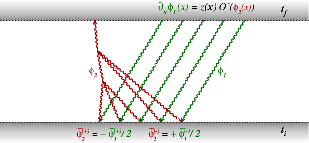
Figure 2: Relationship between the fields $\phi_{1}$ and $\phi_{2}$ in the strong field approximation.

The field $\phi_{1}$ obeys a linear equation of motion (dressed by the field $\phi_{2}$, although this aspect is not visible in the figure), with an advanced boundary condition that depends on $\phi_{2}$. In parallel, the field $\phi_{2}$ obeys a non-linear equation of motion, with a retarded boundary condition that depends on $\phi_{1}$. As we shall show in the next subsection, this tightly constrained problem admits a formal solution, valid to all orders in the function $z$, in the form of an implicit functional equation for the first derivative of $\ln{\cal F}[z]$.

5.2 Formal solution

The equation of motion for $\phi_{1}$ (first of eqs. (71)) is formally identical to the first of eqs. (55). We can therefore mimic eq. (59) and write directly $\phi_{1}$ as follows:

$$\phi_{1}(x)=\int_{\boldsymbol{k}}\int{\rm d}^{3}{\boldsymbol{u}}\;\Big{\{}a_{-{\boldsymbol{k}}}(x)a_{+{\boldsymbol{k}}}(t_{f},{\boldsymbol{u}})-a_{+{\boldsymbol{k}}}(x)a_{-{\boldsymbol{k}}}(t_{f},{\boldsymbol{u}})\Big{\}}\;z({\boldsymbol{u}})\;{\cal O}^{\prime}(\phi_{2}(t_{f},{\boldsymbol{u}}))\;,$$ (72)

where the mode functions $a_{\pm{\boldsymbol{k}}}$ should now be defined with $\phi_{2}$ as the background, rather than $\phi_{2}^{(0)}$. To obtain eq. (72), it was crucial to have a linear equation of motion for $\phi_{1}$, a consequence of the strong field approximation. The above equation formally defines $\phi_{1}(x)$ in the bulk, $x\in\Omega$, in terms of the field $\phi_{2}$ at the final time. It is important to note that this equation is valid to all orders in $z$, contrary to the equations encountered in the expansion in powers of $z$ that we have used in the previous section. Beside the explicit factor $z({\boldsymbol{u}})$, the right hand side contains also an implicit $z$ dependence (to all orders in $z$) in the field $\phi_{2}(t_{f},{\boldsymbol{u}})$ and in the mode functions $a_{\pm{\boldsymbol{k}}}$ (since they evolve on top of the background $\phi_{2}$).

Then, using the boundary condition at the initial time, we obtain the following expression for the field $\phi_{2}$ at $t_{i}$,

$$\phi_{2}(t_{i},{\boldsymbol{y}}) = \frac{1}{2}\int_{\boldsymbol{k}}\int{\rm d}^{3}{\boldsymbol{u}}\;\Big{\{}e^{+ik\cdot y}\,a_{+{\boldsymbol{k}}}(t_{f},{\boldsymbol{u}})$$

$$\quad\qquad\qquad+e^{-ik\cdot y}\,a_{-{\boldsymbol{k}}}(t_{f},{\boldsymbol{u}})\Big{\}}\;z({\boldsymbol{u}})\;{\cal O}^{\prime}(\phi_{2}(t_{f},{\boldsymbol{u}}))$$

$$= \frac{1}{2}\int_{\boldsymbol{k}}\int{\rm d}^{3}{\boldsymbol{u}}\;z({\boldsymbol{u}})\;{\cal O}(\phi_{2}(t_{f},{\boldsymbol{u}}))\;\Big{\{}\stackrel{{\scriptstyle\leftarrow}}{{\mathbbm{T}}}_{+{\boldsymbol{k}}}\,e^{+ik\cdot y}+\stackrel{{\scriptstyle\leftarrow}}{{\mathbbm{T}}}_{-{\boldsymbol{k}}}\,e^{-ik\cdot y}\Big{\}}\;\;,$$

where the arrows indicate on which side the ${\mathbbm{T}}_{\pm{\boldsymbol{k}}}$ operators act. This expression for the field $\phi_{2}$ at the time $t_{i}$ can be used as initial condition for the first of eqs. (71). The next step is to note that the field $\phi_{2}(x)$ that satisfies this equation of motion, and has the initial condition $\phi_{2}(t_{i},{\boldsymbol{y}})$ is formally given by

$$\phi_{2}(x)=\exp\Bigg{\{}\int{\rm d}^{3}{\boldsymbol{y}}\;\phi_{2}(t_{i},{\boldsymbol{y}})\frac{\delta}{\delta\Phi_{\rm ini}(t_{i},{\boldsymbol{y}})}\Bigg{\}}\;\Phi(x)\Bigg{|}_{\Phi_{\rm ini}\equiv 0}\;.$$ (74)

This formula follows from the fact that the derivative $\delta/\delta\Phi_{\rm ini}$ is the generator for shifts of the initial condition of $\Phi$; its exponential is therefore the corresponding translation operator. The same formula applies also to any function of the field, since the exponential operator shifts $\Phi_{\rm ini}$ in any instance of $\Phi$ on its right. In particular, we have

$${\cal O}\big{(}\phi_{2}(x)\big{)}=\exp\Bigg{\{}\int{\rm d}^{3}{\boldsymbol{y}}\;\phi_{2}(t_{i},{\boldsymbol{y}})\frac{\delta}{\delta\Phi_{\rm ini}(t_{i},{\boldsymbol{y}})}\Bigg{\}}\;{\cal O}\big{(}\Phi(x)\big{)}\Bigg{|}_{\Phi_{\rm ini}\equiv 0}\;.$$ (75)

Substituting $\phi_{2}(t_{i},{\boldsymbol{y}})$ by eq. (LABEL:eq:phi2-ti) inside the exponential, this leads to

$${\cal O}\big{(}\phi_{2}(x)\big{)} = \exp\smash{\Bigg{\{}}\frac{1}{2}\int_{\boldsymbol{k}}\int{\rm d}^{3}{\boldsymbol{u}}\;z({\boldsymbol{u}})\,{\cal O}(\phi_{2}(t_{f},{\boldsymbol{u}}))$$ (76)

$$\qquad\qquad\times\Big{[}\stackrel{{\scriptstyle\leftarrow}}{{\mathbbm{T}}}_{+{\boldsymbol{k}}}\stackrel{{\scriptstyle\rightarrow}}{{\mathbbm{T}}}_{-{\boldsymbol{k}}}+\stackrel{{\scriptstyle\leftarrow}}{{\mathbbm{T}}}_{-{\boldsymbol{k}}}\stackrel{{\scriptstyle\rightarrow}}{{\mathbbm{T}}}_{+{\boldsymbol{k}}}\Big{]}\smash{\Bigg{\}}}\;{\cal O}\big{(}\Phi(x)\big{)}\smash{\Bigg{|}}_{\Phi_{\rm ini}\equiv 0}$$

$$= \exp\Bigg{\{}\int{\rm d}^{3}{\boldsymbol{u}}\;z({\boldsymbol{u}})\,{\cal O}(\phi_{2}(t_{f},{\boldsymbol{u}}))\;\otimes\Bigg{\}}\;{\cal O}\big{(}\Phi(x)\big{)}\Bigg{|}_{\Phi_{\rm ini}\equiv 0}\;.$$

Setting $x^{0}=t_{f}$ and denoting

$${\cal D}[{\boldsymbol{x}}_{1};z]\equiv{\cal O}(\phi_{2}(t_{f},{\boldsymbol{x}}_{1}))$$ (77)

the first derivative of $\ln{\cal F}$, we see that it obeys the following recursive formula

$${\cal D}[{\boldsymbol{x}}_{1};z]=\exp\Bigg{\{}\int{\rm d}^{3}{\boldsymbol{u}}\;z({\boldsymbol{u}})\,{\cal D}[{\boldsymbol{u}};z]\;\otimes\Bigg{\}}\;{\cal O}\big{(}\Phi(t_{f},{\boldsymbol{x}}_{1})\big{)}\Bigg{|}_{\Phi_{\rm ini}\equiv 0}\;.$$ (78)

Let us make a technical remark about the scope of the $\stackrel{{\scriptstyle\leftarrow}}{{\mathbbm{T}}}_{\pm{\boldsymbol{k}}}$ derivative (contained in the $\otimes$ product) that acts on the factor ${\cal D}[{\boldsymbol{u}};z]$ inside the exponential.

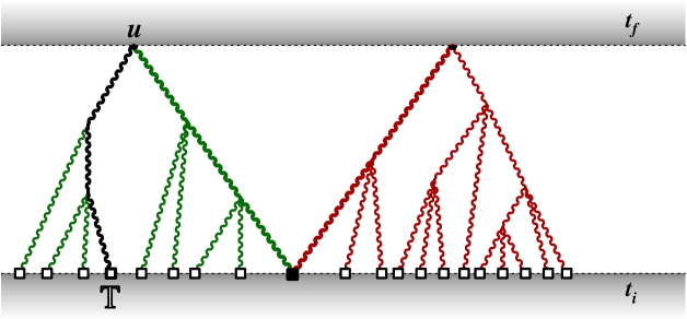
Figure 3: Typical term in $D[{\boldsymbol{u}};z]$ (here we have shown a term with two nodes), showing the tree dependence on the initial field $\Phi_{\rm ini}$ (represented by open squares on the initial time surface). The filled square represents the link between the two nodes, that involves the function of eq. (97). The $\otimes$ product acting on $D[{\boldsymbol{u}};z]$ in eq. (78) acts only on the initial fields that connect to the point ${\boldsymbol{u}}$.

This derivative originates from the terms in $a_{\pm{\boldsymbol{k}}}(t_{f},{\boldsymbol{u}})\,{\cal O}^{\prime}(\phi_{2}(t_{f},{\boldsymbol{u}}))$ in eq. (LABEL:eq:phi2-ti). From this origin, it is clear that $\stackrel{{\scriptstyle\leftarrow}}{{\mathbbm{T}}}_{\pm{\boldsymbol{k}}}$ must establish a link between a point on the initial surface and the point ${\boldsymbol{u}}$ on the final surface, as illustrated in the figure 3, where the black line is the function $a_{\pm{\boldsymbol{k}}}(t_{f},{\boldsymbol{u}})$). As we shall see in the next section, the recursive expansion of eq. (78) leads to a tree structure where the nodes are observables ${\cal O}(\Phi(t_{f},{\boldsymbol{x}}))$. The above discussion tells us that when performing this expansion, the $\otimes$ product should not be “distributed” to all the nodes inside $D[{\boldsymbol{u}};z]$, but applied only to the node of coordinate ${\boldsymbol{u}}$.

5.3 Realization of the strong field approximation

Let us now return on the condition $\phi_{1}\ll\phi_{2}$ , that was used in the derivation of eq. (78), in order to see a posteriori when it is satisfied. To that effect, we can use eq. (72) for $\phi_{1}$. For $\phi_{2}$, the initial condition at $t_{i}$ is given by eq. (LABEL:eq:phi2-ti). For the sake of this discussion, it is sufficient to use a linearized solution for $\phi_{2}$ in the bulk, that reads

$$\phi_{2}(x)\Big{|}_{\rm lin} = \frac{1}{2}\int_{\boldsymbol{k}}\int{\rm d}^{3}{\boldsymbol{u}}\;\Big{\{}a_{-{\boldsymbol{k}}}(x)a_{+{\boldsymbol{k}}}(t_{f},{\boldsymbol{u}})+a_{+{\boldsymbol{k}}}(x)a_{-{\boldsymbol{k}}}(t_{f},{\boldsymbol{u}})\Big{\}}$$ (79)

$$\qquad\qquad\qquad\qquad\qquad\qquad\times\;z({\boldsymbol{u}})\;{\cal O}^{\prime}(\phi_{2}(t_{f},{\boldsymbol{u}}))\;,$$

First of all, a comparison between eqs. (72) and (79) indicates that $\phi_{1}$ and $\phi_{2}$ have the same order in the coupling constant $g$, since they are made of the same building blocks (the only difference is the sign between the two terms of the integrand, and an irrelevant overall factor $\tfrac{1}{2}$).

However, a hierarchy between $\phi_{1}$ and $\phi_{2}$ arises dynamically when the classical solutions of the field equation of motion (52) are unstable. Such instabilities are fairly generic in several quantum field theories; in particular the scalar field theory with a $\phi^{4}$ coupling that we are using as example throughout this paper is known to have a parametric resonance [20, 21]. Since the mode functions $a_{\pm{\boldsymbol{k}}}$ are linearized perturbations on top of the classical field $\phi_{2}$, an instability of the classical solution $\phi_{2}$ is equivalent to the fact that some of the mode functions grow exponentially with time, as $\exp(\mu(x^{0}-t_{i}))$ (where $\mu$ is the Lyapunov exponent). Thus, since eq. (79) is bilinear in the mode functions, we expect that

$$\phi_{2}(x)\Big{|}_{\rm lin}\sim e^{\mu(x^{0}+t_{f}-2t_{i})}\;.$$ (80)

Estimating the magnitude of $\phi_{1}$ requires more care. Indeed, from eqs. (122) in the appendix A, antisymmetric combinations of the mode functions at equal times remain of order $1$ even if individual mode functions grow exponentially with time. Thus, at the final time, we have

$$\phi_{1}(t_{f},{\boldsymbol{x}})\sim 1\quad\mbox{and}\quad\frac{\phi_{2}(t_{f},{\boldsymbol{x}})}{\phi_{1}(t_{f},{\boldsymbol{x}})}\sim e^{2\mu(t_{f}-t_{i})}\gg 1\;,$$ (81)

for sufficiently large $t_{f}-t_{i}$.

In order to estimate the ratio $\phi_{2}/\phi_{1}$ at intermediate times, one may use the following reasoning. The antisymmetric combination of mode functions that enters in eq. (72) is the advanced propagator $G_{{}_{A}}$ in the background $\phi_{2}$. This retarded propagator may also be expressed in terms of a different set of mode functions $b_{\pm{\boldsymbol{k}}}$ defined to be plane waves at the final time $t_{f}$,

$$\Big{[}\square_{x}+m^{2}-{\cal L}^{\prime\prime}_{\rm int}(\phi_{2}(x))\Big{]}\,b_{\pm{\boldsymbol{k}}}(x)=0$$

$$\lim_{x^{0}\to t_{f}}b_{\pm{\boldsymbol{k}}}(x)=e^{\mp ik\cdot x}\;.$$ (82)

In terms of these alternate mode functions, we also have

$$\phi_{1}(x)=\int_{\boldsymbol{k}}\int{\rm d}^{3}{\boldsymbol{u}}\;\Big{\{}b_{-{\boldsymbol{k}}}(x)b_{+{\boldsymbol{k}}}(t_{f},{\boldsymbol{u}})-b_{+{\boldsymbol{k}}}(x)b_{-{\boldsymbol{k}}}(t_{f},{\boldsymbol{u}})\Big{\}}\;z({\boldsymbol{u}})\;{\cal O}^{\prime}(\phi_{2}(t_{f},{\boldsymbol{u}}))\;,$$ (83)

In the presence of instabilities, these backward evolving mode functions grow when $x^{0}$ decreases away from $t_{f}$, as $\exp(\mu(t_{f}-x^{0}))$ (in this sketchy argument, the Lyapunov exponent $\mu$ is assumed here to be the same for the forward and backward mode functions). This implies

$$\phi_{1}(x)\sim e^{\mu(t_{f}-x^{0})}\;,$$ (84)

and the following magnitude for the ratio $\phi_{2}/\phi_{1}$ at intermediate times

$$\frac{\phi_{2}(x)}{\phi_{1}(x)}\sim\frac{e^{\mu(x^{0}+t_{f}-2t_{i})}}{e^{\mu(t_{f}-x^{0})}}\sim e^{2\mu(x^{0}-t_{i})}\;.$$ (85)

Thus, with instabilities and non-zero Lyapunov exponents, the strong field approximation is generically satisfied thanks to the exponential growth of perturbations over the background. In the appendix C, we will discuss another situation where this approximation is also satisfied, namely when the initial state is a mixed state with large occupation number.

5.4 Expansion of eq. (78) in powers of $z$

Although eq. (78) cannot be solved explicitly, it is fairly easy to obtain a diagrammatic representation of its solution. For this, let us introduce the following graphical notations:

$$\equiv \quad{\cal O}\big{(}\Phi(t_{f},{\boldsymbol{x}}_{i})\big{)}\;,$$

$$\equiv \quad\int{\rm d}^{3}{\boldsymbol{u}}\;z({\boldsymbol{u}})\;{\cal O}\big{(}\Phi(t_{f},{\boldsymbol{u}})\big{)}\;,$$

$$\equiv \quad A\otimes B\;.$$

At the order $0$ in $z$, we just need to set $z\equiv 0$ inside the exponential, to obtain

$${\cal D}^{(0)}[{\boldsymbol{x}}_{1};z]=\raise-2.84526pt\hbox to10.32835pt{\leavevmode\resizebox{10.32835pt}{}{\includegraphics{D0}}}\;.$$ (86)

Then, we proceed recursively. We insert the $0$-th order result in the exponential, and expand to order $1$ in $z$, leading to the following result at order $1$:

$${\cal D}^{(1)}[{\boldsymbol{x}}_{1};z]=\raise-2.84526pt\hbox to42.67912pt{\leavevmode\resizebox{42.67912pt}{}{\includegraphics{D1}}}\;.$$ (87)

The next two iterations give:

$${\cal D}^{(2)}[{\boldsymbol{x}}_{1};z]=\raise-2.84526pt\hbox to73.97716pt{\leavevmode\resizebox{73.97716pt}{}{\includegraphics{D2-1}}}+\frac{1}{2!}\,\raise-2.84526pt\hbox to73.97716pt{\leavevmode\resizebox{73.97716pt}{}{\includegraphics{D2-2}}}\;,$$ (88)

and

$${\cal D}^{(3)}[{\boldsymbol{x}}_{1};z] = \raise-2.84526pt\hbox to105.27519pt{\leavevmode\resizebox{105.27519pt}{}{\includegraphics{D3-1}}}+\;\raise-2.84526pt\hbox to105.27519pt{\leavevmode\resizebox{105.27519pt}{}{\includegraphics{D3-2}}}$$ (89)

$$\qquad\quad\vphantom{\Bigg{[}}+\frac{1}{2!}\raise-31.29802pt\hbox to56.9055pt{\leavevmode\resizebox{56.9055pt}{}{\includegraphics{D3-3}}}+\frac{1}{3!}\!\!\raise-31.29802pt\hbox to56.9055pt{\leavevmode\resizebox{56.9055pt}{}{\includegraphics{D3-4}}}\;.$$

These examples generalize to all orders in $z$: the functional ${\cal D}[{\boldsymbol{x}}_{1};z]$ can be represented as the sum of all the rooted trees (the root being the node carrying the fixed point ${\boldsymbol{x}}_{1}$) weighted by the corresponding symmetry factor $1/{\cal S}(T)$:

$$\frac{\delta\ln{\cal F}[z]}{\delta z({\boldsymbol{z}}_{1})}={\cal D}[{\boldsymbol{x}}_{1};z]=\sum_{\mbox{\scriptsize rooted}\atop\mbox{\scriptsize trees }T}\frac{1}{{\cal S}(T)}\;\;\raise-48.36967pt\hbox to106.69783pt{\leavevmode\resizebox{106.69783pt}{}{\includegraphics{tree_example1}}}\;.$$ (90)

Note that the sum of the weights for the trees with $n+1$ nodes (one of them being the root node ${\boldsymbol{x}}_{1}$),

$$w_{n}\equiv\sum_{\mbox{\scriptsize rooted}\atop\mbox{\scriptsize trees }T_{n+1}}\frac{1}{{\cal S}(T_{n+1})}\;,$$ (91)

is the $n$-th Taylor coefficient of the function $w(z)$,

$$w(z)\equiv\sum_{n=0}^{\infty}w_{n}\,z^{n}\;,$$ (92)

that satisfies the following identity

$$w(z)=e^{z\,w(z)}\;.$$ (93)

This functional identity may be viewed as a structureless version of eq. (78), in which the function $z({\boldsymbol{x}})$ is replaced by a scalar variable $z$. Eq. (93) leads to (see [22], pp. 127-128)

$$w_{n}=\frac{(n+1)^{n-1}}{n!}\;,$$ (94)

which is the number of trees with $n+1$ labeled nodes (Cayley’s formula) divided by the number of ways of reshuffling the $n$ nodes that are integrated out.

5.5 Correlation functions

The $n$-point correlation function is obtained by differentiating this expression $n-1$ times, with respect to $z({\boldsymbol{x}}_{2}),\cdots,z({\boldsymbol{x}}_{n})$, and by setting $z\equiv 0$ afterwards. This selects all the trees with $n$ distinct labeled nodes (including the node at ${\boldsymbol{x}}_{1}$). Moreover, since derivatives commute, these successive differentiations eliminate the symmetry factors, leading to

$$\frac{\delta\ln{\cal F}[z]}{\delta z({\boldsymbol{z}}_{1})\cdots\delta z({\boldsymbol{x}}_{n})}\Bigg{|}_{z\equiv 0}={\cal C}_{\{1\cdots n\}}=\sum_{{\mbox{\scriptsize trees with }n}\atop{\mbox{\scriptsize labeled nodes}}}\raise-48.36967pt\hbox to106.69783pt{\leavevmode\resizebox{106.69783pt}{}{\includegraphics{tree_example2}}}\;.$$ (95)

The number of trees contributing to this sum is equal to $n^{n-2}$. Eq. (95) tells us that, at tree level in the strong field regime, all the $n$-point correlation functions are entirely determined by the functional dependence of the solution of the classical field equation of motion with respect to its initial condition. Moreover, this formula provides a way to construct explicitly the correlation functions in terms of functional derivatives with respect to the initial field.

In this tree representation, the number of links reaching a node is the number derivatives with respect to $\Phi_{\rm ini}$ that act on the corresponding ${\cal O}(\Phi)$. When the observable is a composite operator in terms of the fields of the theory, this includes a large number of contributions. For instance, when ${\cal O}(\Phi(x))$ is cubic in the field $\Phi(x)$, a node with three links would contain the following terms:

$${\mathbbm{T}}_{1}{\mathbbm{T}}_{2}{\mathbbm{T}}_{3}\;\raise-8.53581pt\hbox to22.76219pt{\leavevmode\resizebox{22.76219pt}{}{\includegraphics{der1}}}\;\,=\raise-36.41953pt\hbox to41.25648pt{\leavevmode\resizebox{41.25648pt}{}{\includegraphics{der2}}}+\raise-35.56593pt\hbox to32.72066pt{\leavevmode\resizebox{32.72066pt}{}{\includegraphics{der3}}}\;\;+\raise-35.56593pt\hbox to32.72066pt{\leavevmode\resizebox{32.72066pt}{}{\includegraphics{der4}}}\;\;+\raise-35.56593pt\hbox to32.72066pt{\leavevmode\resizebox{32.72066pt}{}{\includegraphics{der5}}}\;\;,$$ (96)

where the three dots inside the blob represent the three fields $\Phi$ it contains. Instead of the functional derivation of the representation (95) that we have performed in this section, one could in principle have iterated on the $z$-expansion introduced in the previous section (after simplifying the equations of motion based on $\phi_{1}\ll\phi_{2}$). This approach produces a sum of terms corresponding to the right hand side of eq. (96) that, after some hefty combinatorics, one may rewrite in the compact form of the left hand side of eq. (96).

In the strong field approximation, the final state correlations are entirely due to quantum fluctuations in the initial state, that are encoded in the function $G_{22}^{0}(x,y)$. If the initial state is the vacuum, as we have assumed in this paper, it reads

$$G_{22}^{0}(x,y)=\int\frac{{\rm d}^{3}{\boldsymbol{k}}}{(2\pi)^{2}2E_{\boldsymbol{k}}}\;e^{i{\boldsymbol{k}}\cdot({\boldsymbol{x}}-{\boldsymbol{y}})}\;.$$ (97)

The support of this function is dominated by distances $|{\boldsymbol{x}}-{\boldsymbol{y}}|$ smaller than the Compton wavelength $m^{-1}$. Thus, in the tree representation of eq. (95), a link between the points ${\boldsymbol{x}}_{i}$ and ${\boldsymbol{x}}_{j}$ is nonzero provided that the past light-cones of summits $x_{i}$ and $x_{j}$ overlap at the initial time (or at least approach each other within distances $\lesssim m^{-1}$), as illustrated in the figure 4.

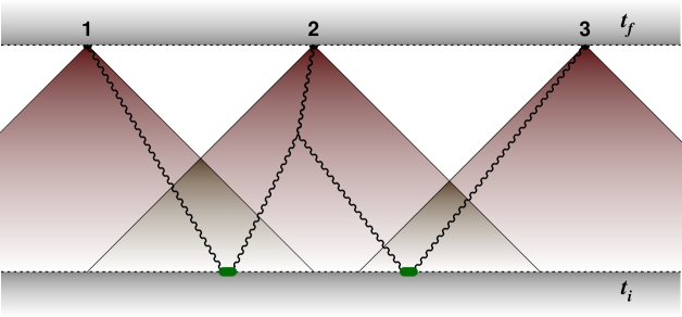
Figure 4: Causal structure of the $3$-point correlation function in the strong field regime.

5.6 Generalizations

Let us list here several extensions, for which the result of eq. (95) would remain valid modulo some minor changes:

• Although we have assumed for simplicity in the derivation that all the observables are evaluated at the same time $t_{f}$, the final result (95) remains valid for measurements at more general spacetime locations $x_{1},\cdots,x_{n}$. The only limitation is that all the separations between these points should be space-like, $(x_{i}-x_{j})^{2}<0$ if $i\not=j$, in order to avoid that the measurement performed at one point influences the outcome of the measurement performed at another point.

• It is possible to evaluate correlation functions where different observables are evaluated at each point $x_{i}$, by having one type of node for each observable in the tree representation of eq. (95).

• One can easily replace the initial vacuum state by any coherent state. Instead of setting the initial field $\Phi_{\rm ini}$ (and its first time derivative) to zero after evaluating the derivatives corresponding to the links in the trees of eq. (95), one would have to set them to the values of $\Phi_{\rm ini}$ and $\partial_{0}\Phi_{\rm ini}$ that correspond to the coherent state of interest (see the appendix B for more details).

• Another extension is to consider a mixed state as initial state. If this state is highly occupied, the strong field approximation is also satisfied, as explained in the appendix C.

6 Beyond the strong field approximation

In the section 4, we have obtained the complete tree level result for the $1$-point (eq. (54)) and $2$-point (eq. (68)) functions, and one readily sees that they coincide with the result of the strong field approximation derived in the previous section (eq. (95) for $n=1$ and $n=2$, respectively). However, as we shall see now, for the $3$-point function and beyond, the strong field approximation does not include all the tree level contributions. This is expected from the fact that the strong field approximation neglects some terms in the equations of motion for the fields $\phi_{1}$ and $\phi_{2}$. In this section, we work out the full tree level result for the $3$-point function, in order to clarify which terms are missed by the strong field approximation. Firstly, let us recall here the result for ${\cal C}_{\{123\}}$ in the strong field approximation:

$${\cal C}_{\{123\}}\Big{|}_{{\rm strong}\atop{\rm field}}=\raise-2.84526pt\hbox to73.97716pt{\leavevmode\resizebox{73.97716pt}{}{\includegraphics{C123-1}}}+\raise-2.84526pt\hbox to73.97716pt{\leavevmode\resizebox{73.97716pt}{}{\includegraphics{C123-2}}}+\raise-2.84526pt\hbox to73.97716pt{\leavevmode\resizebox{73.97716pt}{}{\includegraphics{C123-3}}}\;.$$ (98)

(The first of these contributions corresponds to the figure 4.)

Let us now calculate in full the $3$-point function at tree level, including the contributions that are beyond the strong field approximation. To that effect, we must return to the original equations of motion (35), and expand them to second order in $z$, which leads to

$$\Big{[}\square_{x}\!+\!m^{2}\!+\!\tfrac{g^{2}}{2}\big{(}\phi_{2}^{(0)}(x)\big{)}^{2}\Big{]}\,\phi_{1}^{(2)}(x;{\boldsymbol{x}}_{1},{\boldsymbol{x}}_{2})=0\;,$$

$$\Big{[}\square_{x}\!+\!m^{2}\!+\!\tfrac{g^{2}}{2}\big{(}\phi_{2}^{(0)}(x)\big{)}^{2}\Big{]}\,\phi_{2}^{(2)}(x;{\boldsymbol{x}}_{1},{\boldsymbol{x}}_{2})=-g^{2}\phi_{2}^{(0)}(x)\phi_{2}^{(1)}(x;{\boldsymbol{x}}_{1})\phi_{2}^{(1)}(x;{\boldsymbol{x}}_{2})$$

$$\qquad\qquad\qquad\qquad\qquad\qquad\qquad\underline{-\tfrac{g^{2}}{4}\phi_{2}^{(0)}(x)\phi_{1}^{(1)}(x;{\boldsymbol{x}}_{1})\phi_{1}^{(1)}(x;{\boldsymbol{x}}_{2})}\;,$$ (99)

where we have systematically used the fact that $\phi_{1}^{(0)}\equiv 0$ in order to eliminate a few terms. The underlined term in the second equation is the only one that comes from the $\phi_{1}^{3}\phi_{2}$ interaction term in eq. (30), that we had neglected in the strong field approximation. The boundary conditions obeyed by these second-order coefficients at the final time read

$$\phi_{1}^{(2)}(t_{f},{\boldsymbol{x}};{\boldsymbol{x}}_{1},{\boldsymbol{x}}_{2})=0\;,$$

$$\partial_{0}\phi_{1}^{(2)}(t_{f},{\boldsymbol{x}};{\boldsymbol{x}}_{1},{\boldsymbol{x}}_{2})=\delta({\boldsymbol{x}}-{\boldsymbol{x}}_{1})\,{\cal O}^{\prime\prime}(\phi_{2}^{(0)}(x_{1}))\,\phi_{2}^{(1)}(x,{\boldsymbol{x}}_{2})$$

$$\qquad\qquad\qquad\qquad\quad+\delta({\boldsymbol{x}}-{\boldsymbol{x}}_{2})\,{\cal O}^{\prime\prime}(\phi_{2}^{(0)}(x_{2}))\,\phi_{2}^{(1)}(x,{\boldsymbol{x}}_{1})\;,$$ (100)

while those at the initial time relate their Fourier coefficients as follows

$${\widetilde{\boldsymbol{\phi}}}_{2}^{(2)(+)}({\boldsymbol{k}};{\boldsymbol{x}}_{1},{\boldsymbol{x}}_{2})+\frac{1}{2}\,{\widetilde{\boldsymbol{\phi}}}_{1}^{(2)(+)}({\boldsymbol{k}};{\boldsymbol{x}}_{1},{\boldsymbol{x}}_{2})=0\;,$$

$${\widetilde{\boldsymbol{\phi}}}_{2}^{(2)(-)}({\boldsymbol{k}};{\boldsymbol{x}}_{1},{\boldsymbol{x}}_{2})-\frac{1}{2}\,{\widetilde{\boldsymbol{\phi}}}_{1}^{(2)(-)}({\boldsymbol{k}};{\boldsymbol{x}}_{1},{\boldsymbol{x}}_{2})=0\;.$$ (101)

Let us recall now that the strong field approximation is exact for all the coefficients of lesser order, i.e. $\phi_{1,2}^{(0)}$ and $\phi_{1,2}^{(1)}$. Therefore, since the equation for $\phi_{1}^{(2)}$ does not contain any term coming from the vertex $\phi_{2}\phi_{1}^{3}$, its solution is identical to the result of the strong field approximation. Let us now focus on the equation for $\phi_{2}^{(2)}$. It has the structure of a linear equation of motion with the terms in the right hand side playing the role of source terms, since they do not contain $\phi_{2}^{(2)}$ itself. Therefore, we may decompose the solution as the sum of two terms; a term that solves the homogeneous (i.e. without source) equation and obeys the non-trivial boundary conditions (101), and a term that solves the full equation with a trivial null initial condition:

$$\phi_{2}^{(2)}\equiv\psi_{2}^{(2)}+\xi_{2}^{(2)}\;,$$ (102)

with

$$\Big{[}\square_{x}\!+\!m^{2}\!+\!\tfrac{g^{2}}{2}\big{(}\phi_{2}^{(0)}(x)\big{)}^{2}\Big{]}\,\psi_{2}^{(2)}=0\;,$$

$${\widetilde{\boldsymbol{\psi}}}_{2}^{(2)(+)}+\frac{1}{2}\,{\widetilde{\boldsymbol{\phi}}}_{1}^{(2)(+)}=0\;,\quad{\widetilde{\boldsymbol{\psi}}}_{2}^{(2)(-)}-\frac{1}{2}\,{\widetilde{\boldsymbol{\phi}}}_{1}^{(2)(-)}=0\quad\mbox{(at $t_{i}$)}\;,$$ (103)

and

$$\Big{[}\square_{x}\!+\!m^{2}\!+\!\tfrac{g^{2}}{2}\big{(}\phi_{2}^{(0)}(x)\big{)}^{2}\Big{]}\,\xi_{2}^{(2)}=-g^{2}\phi_{2}^{(0)}\phi_{2}^{(1)}\phi_{2}^{(1)}\underline{-\tfrac{g^{2}}{4}\phi_{2}^{(0)}\phi_{1}^{(1)}\phi_{1}^{(1)}}\;,$$

$$\xi_{2}^{(2)}=\partial_{0}\xi_{2}^{(2)}=0\quad\mbox{(at $t_{i}$)}\;.$$ (104)

Concerning $\psi_{2}^{(2)}$, the equation of motion does not contain any term coming from the $\phi_{2}\phi_{1}^{3}$ vertex, and all the objects that appear in the equation of motion and boundary conditions are exact in the strong field approximation. Therefore, $\psi_{2}^{(2)}$ is itself correctly given by this approximation. For $\xi_{2}^{(2)}$, we can write the following solution:

$$\xi_{2}^{(2)}(x;{\boldsymbol{x}}_{1},{\boldsymbol{x}}_{2})=-g^{2}\int{\rm d}^{4}y\;G_{{}_{R}}(x,y)\,\phi_{2}^{(0)}(y)\Big{[}\phi_{2}^{(1)}(y;{\boldsymbol{x}}_{1})\phi_{2}^{(1)}(y;{\boldsymbol{x}}_{2})$$

$$\qquad\qquad\qquad\qquad\qquad\qquad\qquad+\underline{\tfrac{1}{4}\phi_{1}^{(1)}(y;{\boldsymbol{x}}_{1})\phi_{1}^{(1)}(y;{\boldsymbol{x}}_{2})}\Big{]}\;,$$ (105)

where $G_{{}_{R}}(x,y)$ is the retarded propagator dressed by the background field $\phi_{2}^{(0)}$. The first term is already contained in the strong field approximation since it does not involve the $\phi_{2}\phi_{1}^{3}$ vertex, but the second term is present only beyond this approximation. Therefore, the only tree level term in the $3$-point correlation function that is not contained in the strong field approximation is

$${\cal C}_{\{123\}}\Big{|}_{{\rm beyond}\atop{\rm SFA}} = -\frac{ig^{2}}{4}\;{\cal O}^{\prime}(\phi_{2}^{(0)}(x_{1})){\cal O}^{\prime}(\phi_{2}^{(0)}(x_{2})){\cal O}^{\prime}(\phi_{2}^{(0)}(x_{3}))$$ (106)

$$\qquad\times\int{\rm d}^{4}y\;G_{{}_{R}}(x_{3},y)\,\phi_{2}^{(0)}(y)\phi_{1}^{(1)}(y;{\boldsymbol{x}}_{1})\phi_{1}^{(1)}(y;{\boldsymbol{x}}_{2})$$

$$= \frac{ig^{2}}{4}\;{\cal O}^{\prime}(\phi_{2}^{(0)}(x_{1})){\cal O}^{\prime}(\phi_{2}^{(0)}(x_{2})){\cal O}^{\prime}(\phi_{2}^{(0)}(x_{3}))$$

$$\qquad\times\int{\rm d}^{4}y\;G_{{}_{R}}(x_{1},y)G_{{}_{R}}(x_{2},y)G_{{}_{R}}(x_{3},y)\,\phi_{2}^{(0)}(y)\;,$$

where we have used the explicit form (59) of $\phi_{1}^{(1)}$ in order to rewrite it in a completely symmetric form in the second equality. The peculiarity of this contribution is that the correlation is created in the bulk by the self-interactions of the fields, instead of the pairwise initial state correlations that we have encountered in the strong field approximation. Generalizing the diagrammatic representation of eq. (95), such a term may be represented as follows:

$${\cal C}_{\{123\}}\Big{|}_{{\rm beyond}\atop{\rm SFA}}=\;\raise-19.91692pt\hbox to38.41121pt{\leavevmode\resizebox{38.41121pt}{}{\includegraphics{C123-bsfr}}}\;.$$ (107)

(Note that in this representation, the power of the classical field $\phi_{2}^{(0)}(y)$ that accompanies the vertex does not appear explicitly.) The causal structure of this term is illustrated in the figure 5:

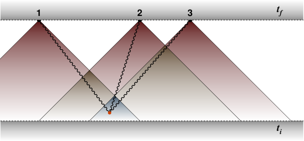
Figure 5: Causal structure of the extra contribution to the $3$-point correlation function that arises beyond the strong field approximation. In this contribution, the correlation is produced in the bulk, from the vertex $\phi_{1}^{3}\phi_{2}$. Causality implies that this vertex must be located in the intersection of the three light-cones. The red dot contains a power of the classical field $\phi_{2}^{(0)}(y)$.

because of the three retarded propagators, the vertex $y$ must be located inside the overlap of the three past light-cones of summits $x_{1,2,3}$, but it is not tied to the initial surface.

To close this section, let us compare the orders of magnitude of the contributions of eq. (98) and of eq. (107) in the presence of the instabilities discussed in the section 5.3. On the one hand, we have

$$\raise-2.84526pt\hbox to73.97716pt{\leavevmode\resizebox{73.97716pt}{}{\includegraphics{C123-1}}}\sim\;g^{4}\;e^{4\mu(t_{f}-t_{i})}\;,$$ (108)

where the factor $g^{4}$ is relative to the completely disconnected $3$-point function (each derivative $\delta/\delta\Phi_{\rm ini}$ brings a factor $g$ when the background field $\Phi$ is of order $g^{-1}$). Regarding the contribution of eq. (107), each link brings a factor $g$ since it replaces a field $\Phi$, and the factor $g^{2}\,\phi_{2}^{(0)}$ is of order $g$. Regarding the time dependence, each retarded propagator behaves as

$$G_{{}_{R}}(x_{1},y)\sim e^{\mu(t_{f}-y^{0})}\;.$$ (109)

Therefore, we have

$$\raise-19.91692pt\hbox to38.41121pt{\leavevmode\resizebox{38.41121pt}{}{\includegraphics{C123-bsfr}}}\sim\;g^{4}\;e^{3\mu(t_{f}-y^{0})}\lesssim g^{4}\;e^{3\mu(t_{f}-t_{i})}\;.$$ (110)

We see that the terms beyond the strong field approximation have the same order in $g$, but are exponentially suppressed by a factor of order $\exp(-\mu(t_{f}-t_{i}))$.

7 Summary and conclusions

In this paper, we have studied the correlation function between an arbitrary number of observables measured at equal times (or more generally at points with space-like separations) in quantum field theory. Our main focus has been the strong field regime, that arises for instance when the fields are driven by a large external source and their classical equations of motion are subject to instabilities.

Firstly, we have constructed a generating functional that encapsulates all these correlation functions by coupling the observables to a fictitious source $z({\boldsymbol{x}})$. Using the retarded-advanced basis of the in-in formalism, we have shown that it can be expressed at tree level in terms of a pair of fields that obey coupled equations of motion and non-trivial boundary conditions that depend on the observables. At the first two orders in the fictitious source (i.e. for the $1$-point and $2$-point correlation functions), the results can be expressed in terms of the retarded classical solution of the field equation of motion, and its functional derivative with respect to its initial condition.

For these two lowest orders, the result we have obtained is in fact exact at tree level, and does not rely on having strong fields. Beyond these low orders, this direct approach is very cumbersome to extend systematically. In order to circumvent this difficulty, we have introduced the strong field approximation, thanks to which one can formally solve the equations of motion with the appropriate boundary conditions, in the form of an implicit functional equation for the first derivative of the generating functional. From this functional relation, we have found that all the correlation functions are expressible in terms of the classical field and its derivatives with respect to the initial condition, generalizing the results for the $1$-point and $2$-point functions. Moreover, the expressions can be systematically represented by trees, where the nodes are the observables and the links are pairs of derivatives with respect to the initial condition of the classical field. Physically, these links correspond to correlations induced by fluctuations in the initial state.

In the last section, we departed from the strong field approximation and considered the tree-level $3$-point correlation function in full. We found an additional tree-level term that does not exist in the strong field regime, corresponding to correlations created in the bulk by the interactions themselves. We expect that such terms (and more complicated ones) exist in all $n$-point tree-level correlation functions for any $n\geq 3$, beyond the strong field regime.

Appendix A Some properties of the mode functions

In the section 4.3.2, we have introduced a basis of solutions for the linear space of solutions for a partial differential equation of the form

$$\Big{[}\square_{x}+m^{2}-{\cal L}^{\prime\prime}_{\rm int}(\varphi(x))\Big{]}\,a(x)=0\;,$$ (111)

where $\varphi(x)$ is some real background field. This basis was defined as a set of solutions $\{a_{\pm{\boldsymbol{k}}}(x)\}$ labeled by a momentum ${\boldsymbol{k}}$, whose initial condition is a plane wave of positive (in the case of $a_{+{\boldsymbol{k}}}$) or negative (in the case of $a_{-{\boldsymbol{k}}}$) frequency:

$$a_{\pm{\boldsymbol{k}}}(x)\mathrel{\mathop{\kern 0.0pt\to}\limits_{x^{0}\to t_{i}}}e^{\mp ik\cdot x}\;.$$ (112)

Any solution of the equation (111) is a linear superposition of the functions $a_{\pm{\boldsymbol{k}}}$.

Given a solution $a(x)$, let us define the following two components vectors

$$\big{|}{\boldsymbol{a}}\big{)}\equiv\begin{pmatrix}a\\ \dot{a}\end{pmatrix}\;,\qquad\big{(}{\boldsymbol{a}}\big{|}\equiv i\begin{pmatrix}-\dot{a}^{*}&a^{*}\end{pmatrix}\;.$$ (113)

Then, from two solutions $a_{1}$ and $a_{2}$ of eq. (111), we may define the following inner product

$$\big{(}{\boldsymbol{a}}_{1}\big{|}{\boldsymbol{a}}_{2}\big{)}\equiv i\int d^{3}{\boldsymbol{x}}\;\Big{[}a_{1}^{*}(x)\,\dot{a}_{2}(x)-\dot{a}_{1}^{*}(x)\,a_{2}(x)\Big{]}\;,$$ (114)

reminiscent of the Wronskian for solutions of ordinary differential equations. This product is Hermitian,

$$\big{(}{\boldsymbol{a}}_{2}\big{|}{\boldsymbol{a}}_{1}\big{)}=\big{(}{\boldsymbol{a}}_{1}\big{|}{\boldsymbol{a}}_{2}\big{)}^{*}\;,$$ (115)

and constant in time:

$$\partial_{0}\big{(}{\boldsymbol{a}}_{1}\big{|}{\boldsymbol{a}}_{2}\big{)}=0\;.$$ (116)

Its value is therefore completely determined by the initial conditions for the solutions $a_{1}$ and $a_{2}$. In the case of the solutions $a_{\pm{\boldsymbol{k}}}$ introduced above, an explicit calculation gives

$$\big{(}{\boldsymbol{a}}_{+{\boldsymbol{k}}}\big{|}{\boldsymbol{a}}_{+{\boldsymbol{k}}^{\prime}}\big{)}=(2\pi)^{3}\,2E_{\boldsymbol{k}}\,\delta({\boldsymbol{k}}-{\boldsymbol{k}}^{\prime})\;,$$

$$\big{(}{\boldsymbol{a}}_{-{\boldsymbol{k}}}\big{|}{\boldsymbol{a}}_{-{\boldsymbol{k}}^{\prime}}\big{)}=-(2\pi)^{3}\,2E_{\boldsymbol{k}}\,\delta({\boldsymbol{k}}-{\boldsymbol{k}}^{\prime})\;,$$

$$\big{(}{\boldsymbol{a}}_{+{\boldsymbol{k}}}\big{|}{\boldsymbol{a}}_{-{\boldsymbol{k}}^{\prime}}\big{)}=0\;.$$ (117)

A generic solution $a$ of eq. (111) can be decomposed as follows

$$\big{|}{\boldsymbol{a}}\big{)}=\int\frac{{\rm d}^{3}{\boldsymbol{k}}}{(2\pi)^{3}2E_{\boldsymbol{k}}}\;\Big{[}\gamma_{+{\boldsymbol{k}}}\;\big{|}{\boldsymbol{a}}_{+{\boldsymbol{k}}}\big{)}+\gamma_{-{\boldsymbol{k}}}\;\big{|}{\boldsymbol{a}}_{-{\boldsymbol{k}}}\big{)}\Big{]}\;,$$ (118)

and from the inner products between the mode functions we readily see that the coefficients of this linear decomposition are given by

$$\gamma_{+{\boldsymbol{k}}}=\big{(}{\boldsymbol{a}}_{+{\boldsymbol{k}}}\big{|}{\boldsymbol{a}}\big{)}\;,\quad\gamma_{-{\boldsymbol{k}}}=-\big{(}{\boldsymbol{a}}_{-{\boldsymbol{k}}}\big{|}{\boldsymbol{a}}\big{)}\;.$$ (119)

Note that in the decomposition (118), the coefficients $\gamma_{\pm{\boldsymbol{k}}}$ are constant, and the time dependence is carried by the mode functions $a_{\pm{\boldsymbol{k}}}$. Therefore, we can write

$$\big{|}{\boldsymbol{a}}\big{)}=\int\frac{{\rm d}^{3}{\boldsymbol{k}}}{(2\pi)^{3}2E_{\boldsymbol{k}}}\;\Big{[}\big{|}{\boldsymbol{a}}_{+{\boldsymbol{k}}}\big{)}\big{(}{\boldsymbol{a}}_{+{\boldsymbol{k}}}\big{|}{\boldsymbol{a}}\big{)}-\big{|}{\boldsymbol{a}}_{-{\boldsymbol{k}}}\big{)}\big{(}{\boldsymbol{a}}_{-{\boldsymbol{k}}}\big{|}{\boldsymbol{a}}\big{)}\Big{]}\;.$$ (120)

Since this is true for any solution $a$, the following relationship must in fact be true

$$\int\frac{{\rm d}^{3}{\boldsymbol{k}}}{(2\pi)^{3}2E_{\boldsymbol{k}}}\;\Big{[}\big{|}{\boldsymbol{a}}_{+{\boldsymbol{k}}}\big{)}\big{(}{\boldsymbol{a}}_{+{\boldsymbol{k}}}\big{|}-\big{|}{\boldsymbol{a}}_{-{\boldsymbol{k}}}\big{)}\big{(}{\boldsymbol{a}}_{-{\boldsymbol{k}}}\big{|}\Big{]}=\begin{pmatrix}1&0\\ 0&1\\ \end{pmatrix}\;.$$ (121)

Reinstating coordinates, this identity reads

$$\int_{k}\begin{pmatrix}a_{+{\boldsymbol{k}}}(x)\dot{a}_{-{\boldsymbol{k}}}(y)-a_{-{\boldsymbol{k}}}(x)\dot{a}_{+{\boldsymbol{k}}}(y)&a_{-{\boldsymbol{k}}}(x)a_{+{\boldsymbol{k}}}(y)-a_{+{\boldsymbol{k}}}(x)a_{-{\boldsymbol{k}}}(y)\\ \dot{a}_{+{\boldsymbol{k}}}(x)\dot{a}_{-{\boldsymbol{k}}}(y)-\dot{a}_{-{\boldsymbol{k}}}(x)\dot{a}_{+{\boldsymbol{k}}}(y)&\dot{a}_{-{\boldsymbol{k}}}(x)a_{+{\boldsymbol{k}}}(y)-\dot{a}_{+{\boldsymbol{k}}}(x)a_{-{\boldsymbol{k}}}(y)\\ \end{pmatrix}$$

$$\qquad\qquad\qquad\qquad\qquad\mathrel{\mathop{\kern 0.0pt=}\limits_{x^{0}=y^{0}}}i\,\delta({\boldsymbol{x}}-{\boldsymbol{y}})\begin{pmatrix}1&0\\ 0&1\\ \end{pmatrix}\;.$$ (122)

These identities are justification for eqs. (59) and (72).

Appendix B In-in formalism for an initial coherent state

A coherent state can be defined from the perturbative in-vacuum as follows

$$\big{|}\chi\big{>}\equiv{\cal N}_{\chi}\;\exp\Big{\{}\int_{\boldsymbol{k}}\chi({\boldsymbol{k}})\,a_{\rm in}^{\dagger}({\boldsymbol{k}})\Big{\}}\;\big{|}0{}_{\rm in}\big{>}\;,$$ (123)

where $\chi({\boldsymbol{k}})$ is a function of 3-momentum and ${\cal N}_{\chi}$ a normalization constant adjusted so that $\big{<}\chi\big{|}\chi\big{>}=1$. From the canonical commutation relation

$$\big{[}a_{\rm in}({\boldsymbol{p}}),a_{\rm in}^{\dagger}({\boldsymbol{q}})\big{]}=(2\pi)^{3}\,2E_{\boldsymbol{p}}\,\delta({\boldsymbol{p}}-{\boldsymbol{q}})\;,$$ (124)

it is easy to check the following

$$a_{\rm in}({\boldsymbol{p}})\,\big{|}\chi\big{>}=\chi({\boldsymbol{p}})\,\big{|}\chi\big{>}\;,$$

$$\big{|}{\cal N}_{\chi}\big{|}^{2}=\exp\Big{\{}-\int_{\boldsymbol{k}}\big{|}\chi({\boldsymbol{k}})\big{|}^{2}\Big{\}}\;.$$ (125)

The first equation tells us that $\big{|}\chi\big{>}$ is an eigenstate of annihilation operators, which is another definition of coherent states, and the second one provides the value of the normalization constant.

Consider now the generating functional for the in-in formalism in this coherent state,

$$Z_{\chi}[\eta] \equiv \big{<}\chi\big{|}{\rm P}\,\exp i\int_{\cal C}{\rm d}^{4}x\;\eta(x)\phi(x)\big{|}\chi\big{>}$$ (126)

$$= \big{<}\chi\big{|}{\rm P}\,\exp i\int_{\cal C}{\rm d}^{4}x\;\Big{[}{\cal L}_{\rm int}(\phi_{\rm in}(x))+\eta(x)\phi_{\rm in}(x)\Big{]}\big{|}\chi\big{>}\;,$$

where $\eta(x)$ is a fictitious source that lives on the closed-time contour ${\cal C}$ introduced after eq. (13). The first step is to factor out the interactions as follows:

$$Z_{\chi}[\eta]=\exp i\int_{\cal C}{\rm d}^{4}x\;{\cal L}_{\rm int}\Big{(}\frac{\delta}{i\delta\eta(x)}\Big{)}\;\underbrace{\big{<}\chi\big{|}{\rm P}\,\exp i\int_{\cal C}{\rm d}^{4}x\;\eta(x)\phi_{\rm in}(x)\big{|}\chi\big{>}}_{Z_{\chi 0}[\eta]}\;.$$ (127)

A first use of the Baker-Campbell-Hausdorff formula enables one to remove the path ordering, giving

$$Z_{\chi 0}[\eta]=\big{<}\chi\big{|}\exp i\int_{\cal C}{\rm d}^{4}x\;\eta(x)\phi_{\rm in}(x)\big{|}\chi\big{>}$$

$$\quad\times\exp\Big{\{}-\frac{1}{2}\int_{\cal C}{\rm d}^{4}x{\rm d}^{4}y\;\eta(x)\eta(y)\;\theta_{c}(x^{0}-y^{0})\;\big{[}\phi_{\rm in}(x),\phi_{\rm in}(y)\big{]}\Big{\}}\;,$$ (128)

where $\theta_{c}(x^{0}-y^{0})$ generalizes the step function to the ordered contour ${\cal C}$. Note that the factor on the second line is a commuting number and thus can be removed from the expectation value. A second application of the Baker-Campbell-Hausdorff formula allows to normal-order the first factor. Decomposing the in-field as follows,

$$\phi_{\rm in}(x)\equiv\underbrace{\int_{\boldsymbol{k}}a_{\rm in}({\boldsymbol{k}})\,e^{-ik\cdot x}}_{\phi_{\rm in}^{(-)}(x)}+\underbrace{\int_{\boldsymbol{k}}a_{\rm in}^{\dagger}({\boldsymbol{k}})\,e^{+ik\cdot x}}_{\phi_{\rm in}^{(+)}(x)}\;,$$ (129)

we obtain

$$Z_{\chi 0}[\eta]=\big{<}\chi\big{|}\exp\Big{\{}i\int_{\cal C}{\rm d}^{4}x\;\eta(x)\phi_{\rm in}^{(+)}(x)\Big{\}}\exp\Big{\{}i\int_{\cal C}{\rm d}^{4}y\;\eta(y)\phi_{\rm in}^{(-)}(y)\Big{\}}\big{|}\chi\big{>}$$

$$\quad\times\exp\Big{\{}+\frac{1}{2}\int_{\cal C}{\rm d}^{4}x{\rm d}^{4}y\;\eta(x)\eta(y)\,\big{[}\phi_{\rm in}^{(+)}(x),\phi_{\rm in}^{(-)}(y)\big{]}\Big{\}}$$

$$\quad\times\exp\Big{\{}-\frac{1}{2}\int_{\cal C}{\rm d}^{4}x{\rm d}^{4}y\;\eta(x)\eta(y)\;\theta_{c}(x^{0}-y^{0})\;\big{[}\phi_{\rm in}(x),\phi_{\rm in}(y)\big{]}\Big{\}}\;.$$ (130)

The factor of the first line can be evaluated by using the fact that the coherent state is an eigenstate of annihilation operators:

$$\big{<}\chi\big{|}\exp\Big{\{}i\int_{\cal C}{\rm d}^{4}x\;\eta(x)\phi_{\rm in}^{(+)}(x)\Big{\}}\exp\Big{\{}i\int_{\cal C}{\rm d}^{4}y\;\eta(y)\phi_{\rm in}^{(-)}(y)\Big{\}}\big{|}\chi\big{>}$$

$$\quad=\exp\Big{\{}i\int_{\cal C}{\rm d}^{4}x\;\eta(x)\;\underbrace{\int_{\boldsymbol{k}}\Big{(}\chi({\boldsymbol{k}})e^{-ik\cdot x}+\chi^{*}({\boldsymbol{k}})e^{+ik\cdot x}\Big{)}}_{\Phi_{\chi}(x)}\Big{\}}\;.$$ (131)

We denote $\Phi_{\chi}(x)$ the field obtained by substituting the creation and annihilation operators of the in-field by $\chi^{*}({\boldsymbol{k}})$ and $\chi({\boldsymbol{k}})$ respectively. Note that this is no longer an operator, but a (real valued) commuting field. Moreover, because it is a linear superposition of plane waves, this field is a free field:

$$(\square_{x}+m^{2})\,\Phi_{\chi}(x)=0\;.$$ (132)

The second and third factors of eq. (130) are commuting numbers, provided we do not attempt to disassemble the commutators. Using the decomposition of the in-field in terms of creation and annihilation operators, and the canonical commutation relation of the latter, we obtain

$$\theta_{c}(x^{0}-y^{0})\;\big{[}\phi_{\rm in}(x),\phi_{\rm in}(y)\big{]}-\big{[}\phi_{\rm in}^{(+)}(x),\phi_{\rm in}^{(-)}(y)\big{]}$$

$$\qquad=\underbrace{\theta_{c}(x^{0}-y^{0})\int_{\boldsymbol{k}}e^{-ik\cdot(x-y)}+\theta_{c}(y^{0}-x^{0})\int_{\boldsymbol{k}}e^{+ik\cdot(x-y)}}_{G_{c}^{0}(x,y)}\;,$$ (133)

which is nothing but the usual bare path-ordered propagator $G_{c}^{0}(x,y)$. Collecting all the factors, the generating functional for path-ordered Green’s functions in the in-in formalism with an initial coherent state reads

$$Z_{\chi}[\eta] = \exp\Big{\{}i\int_{\cal C}{\rm d}^{4}x\;{\cal L}_{\rm int}\Big{(}\frac{\delta}{i\delta\eta(x)}\Big{)}\Big{\}}\;\underline{\exp\Big{\{}i\int_{\cal C}{\rm d}^{4}x\;\eta(x)\,\Phi_{\chi}(x)\Big{\}}}$$ (134)

$$\qquad\times\exp\Big{\{}-\frac{1}{2}\int_{\cal C}{\rm d}^{4}x{\rm d}^{4}y\;\eta(x)\eta(y)\;G_{c}^{0}(x,y)\Big{\}}\;.$$

We see that it differs from the corresponding functional with the perturbative vacuum as initial state only by the second factor, that we have underlined. This generating functional is also equal to

$$Z_{\chi}[\eta] = \exp\Big{\{}i\int_{\cal C}{\rm d}^{4}x\;\eta(x)\,\Phi_{\chi}(x)\Big{\}}\;\exp\Big{\{}i\int_{\cal C}{\rm d}^{4}x\;{\cal L}_{\rm int}\Big{(}\Phi_{\chi}(x)+\frac{\delta}{i\delta\eta(x)}\Big{)}\Big{\}}\;$$ (135)

$$\qquad\times\exp\Big{\{}-\frac{1}{2}\int_{\cal C}{\rm d}^{4}x{\rm d}^{4}y\;\eta(x)\eta(y)\;G_{c}^{0}(x,y)\Big{\}}\;.$$

The first factor amounts to shifting the fields by $\Phi_{\chi}(x)$. The simplest way to see this is to write

$$\phi\equiv\Phi_{\chi}+\zeta\;.$$ (136)

In the definition (126), this leads to

$$Z_{\chi}[\eta]=\exp\Big{\{}i\int_{\cal C}{\rm d}^{4}\;\eta(x)\,\Phi_{\chi}(x)\Big{\}}\;\big{<}\chi\big{|}{\rm P}\,\exp i\int_{\cal C}{\rm d}^{4}x\;\eta(x)\,\zeta(x)\big{|}\chi\big{>}\;,$$ (137)

where the second factor in the right hand side is the generating functional for correlators of $\zeta$. Comparing with eq. (135), we see that the generating functional for $\zeta$ is identical to the vacuum one, except that the argument $\phi$ of the interaction Lagrangian is replaced by $\Phi_{\chi}+\zeta$:

$${\cal L}_{\rm int}(\phi)\quad\to\quad{\cal L}_{\rm int}(\Phi_{\chi}+\zeta)\;.$$ (138)

In other words, the field $\zeta$ appears to be coupled to an external source and to a background field. Note that in the in-in formalism, the change $\phi\to\Phi_{\chi}+\zeta$ applies equally to the fields $\phi_{\pm}$ on both branches of the time contour. Therefore, for the fields $\phi_{1,2}$ in the retarded-advanced basis, we have

$$\phi_{1}=\zeta_{1}\quad,\qquad\phi_{2}=\Phi_{\chi}+\zeta_{2}\;,$$ (139)

and the integral equations (28) that determine these fields at tree level become

$$\zeta_{1}(x) = i\int_{\Omega}{\rm d}^{4}y\;G_{12}^{0}(x,y)\,\frac{\partial{\boldsymbol{L}}_{\rm int}(\zeta_{1},\Phi_{\chi}+\zeta_{2})}{\partial\zeta_{2}(y)}$$

$$\qquad+\int_{t_{f}}{\rm d}^{3}{\boldsymbol{y}}\;G_{12}^{0}(x,y)\;z({\boldsymbol{y}})\;{\cal O}^{\prime}(\Phi_{\chi}(y)+\zeta_{2}(y))\;,$$

$$\zeta_{2}(x) = i\int_{\Omega}{\rm d}^{4}y\;\Big{\{}G_{21}^{0}(x,y)\frac{\partial{\boldsymbol{L}}_{\rm int}(\zeta_{1},\Phi_{\chi}\!+\!\zeta_{2})}{\partial\zeta_{1}(y)}\!+\!G_{22}^{0}(x,y)\frac{\partial{\boldsymbol{L}}_{\rm int}(\zeta_{1},\Phi_{\chi}\!+\!\zeta_{2})}{\partial\zeta_{2}(y)}\Big{\}}$$ (140)

$$\qquad+\int_{t_{f}}{\rm d}^{3}{\boldsymbol{y}}\;G_{22}^{0}(x,y)\;z({\boldsymbol{y}})\;{\cal O}^{\prime}(\Phi_{\chi}(y)+\zeta_{2}(y))\;.$$

Using $\phi_{2}=\Phi_{\chi}+\zeta_{2}$ and the fact that $\Phi_{\chi}$ is a free field, we see that the equations of motion corresponding to these integral equations are the same as eqs. (34). The boundary conditions at the final time read:

$$\zeta_{1}(t_{f},{\boldsymbol{x}})=0\quad,\qquad\partial_{0}\zeta_{1}(t_{t},{\boldsymbol{x}})=i\,z({\boldsymbol{x}})\,{\cal O}^{\prime}\big{(}\Phi_{\chi}(t_{f},{\boldsymbol{x}})+\zeta_{2}(t_{f},{\boldsymbol{x}})\big{)}\;,$$ (141)

while at the initial time we have the following relationship

$${\widetilde{\boldsymbol{\zeta}}}_{2}^{(+)}({\boldsymbol{k}})=-\frac{1}{2}\,{\widetilde{\boldsymbol{\zeta}}}_{1}^{(+)}({\boldsymbol{k}})\;,\quad{\widetilde{\boldsymbol{\zeta}}}_{2}^{(-)}({\boldsymbol{k}})=\frac{1}{2}\,{\widetilde{\boldsymbol{\zeta}}}_{1}^{(-)}({\boldsymbol{k}})$$ (142)

among the Fourier coefficients. The derivation of the main result (78) for a vacuum initial state can be reproduced almost identically for a coherent initial state, leading to

$${\cal D}[{\boldsymbol{x}}_{1};z]=\exp\Bigg{\{}\int{\rm d}^{3}{\boldsymbol{u}}\;z({\boldsymbol{u}})\,{\cal D}[{\boldsymbol{u}};z]\;\otimes\Bigg{\}}\;{\cal O}\big{(}\Phi(t_{f},{\boldsymbol{x}}_{1})\big{)}\Bigg{|}_{\Phi_{\rm ini}\equiv\Phi_{\chi}}\;,$$ (143)

the only difference being that the initial value of the classical field $\Phi$ is set to $\Phi_{\chi}$ instead of zero after the derivatives with respect to $\Phi_{\rm ini}$ have been performed.

Appendix C In-in formalism for a Gaussian mixed state

Let us consider in this section a mixed initial state described by the following density matrix

$$\rho\equiv\exp\Big{\{}-\int_{\boldsymbol{k}}\beta_{\boldsymbol{k}}E_{\boldsymbol{k}}\,a^{\dagger}_{\rm in}({\boldsymbol{k}})a_{\rm in}({\boldsymbol{k}})\Big{\}}\;.$$ (144)

In this definition, $\beta_{\boldsymbol{k}}$ has the same function as an inverse temperature (by allowing it to be momentum dependent we can also consider out-of-equilibrium systems). The expectation value in the pure initial state of eq. (9) is replaced by a trace

$$\big{<}0{}_{\rm in}\big{|}\cdots\big{|}0{}_{\rm in}\big{>}\quad\to\quad\frac{{\rm Tr}\,\big{(}\rho\cdots\big{)}}{{\rm Tr}\,\big{(}\rho\big{)}}\;.$$ (145)

How to handle this type of initial state is well known from quantum field theory at finite temperature. The perturbative rules are identical to those exposed in the figure 1, but the propagators of eqs. (14) should be replaced by

$$G_{-+}^{0}(x,y)=\int_{\boldsymbol{k}}\Big{(}(1+f_{\boldsymbol{k}})\,e^{-ik\cdot(x-y)}+f_{\boldsymbol{k}}\,e^{ik\cdot(x-y)}\Big{)}\;,$$

$$G_{+-}^{0}(x,y)=\int_{\boldsymbol{k}}\Big{(}f_{\boldsymbol{k}}\,e^{-ik\cdot(x-y)}+(1+f_{\boldsymbol{k}})\,e^{ik\cdot(x-y)}\Big{)}\;,$$

$$G_{++}^{0}(x,y)=\theta(x^{0}-y^{0})\,G_{-+}^{0}(x,y)+\theta(y^{0}-x^{0})\,G_{+-}^{0}(x,y)\;,$$

$$G_{--}^{0}(x,y)=\theta(x^{0}-y^{0})\,G_{+-}^{0}(x,y)+\theta(y^{0}-x^{0})\,G_{-+}^{0}(x,y)\;,$$ (146)

where we have defined

$$f_{\boldsymbol{k}}\equiv\frac{1}{e^{\beta_{\boldsymbol{k}}E_{\boldsymbol{k}}}-1}\;.$$ (147)

In the retarded-advanced basis, the propagators $G_{12}^{0}$ and $G_{21}^{0}$ are unmodified, but the propagator $G_{22}^{0}$ becomes $f_{\boldsymbol{k}}$-dependent. The integral equations (28) are unaltered (but they acquire a hidden dependence on $f_{\boldsymbol{k}}$ through $G_{22}^{0}$), and consequently the equations of motion (34) are unchanged. The boundary conditions (41) at the final time remain the same, but those at the initial time (45) are modified into

$${\widetilde{\boldsymbol{\phi}}}_{2}^{(+)}({\boldsymbol{k}})=-\Big{(}\frac{1}{2}+f_{\boldsymbol{k}}\Big{)}\,{\widetilde{\boldsymbol{\phi}}}_{1}^{(+)}({\boldsymbol{k}})\;,\quad{\widetilde{\boldsymbol{\phi}}}_{2}^{(-)}({\boldsymbol{k}})=\Big{(}\frac{1}{2}+f_{\boldsymbol{k}}\Big{)}\,{\widetilde{\boldsymbol{\phi}}}_{1}^{(-)}({\boldsymbol{k}})\;.$$ (148)

In other words, the factor $\tfrac{1}{2}$ of eqs. (45), that can be interpreted as the zero point occupation of the vacuum, is now replaced by the total occupation number $\tfrac{1}{2}+f_{\boldsymbol{k}}$ of the mixed initial state under consideration. We see from eqs. (148) that a large occupation number enhances $\phi_{2}$ with respect to $\phi_{1}$. This is another situation where the strong field approximation introduced in the section 5 is applicable.

References

- [1] V. F. Mukhanov, H. A. Feldman, and R. H. Brandenberger, “Theory of cosmological perturbations. Part 1. Classical perturbations. Part 2. Quantum theory of perturbations. Part 3. Extensions,” Phys. Rept. 215 (1992) 203–333.
- [2] S. Weinberg, “Quantum contributions to cosmological correlations,” Phys. Rev. D72 (2005) 043514, arXiv:hep-th/0506236 [hep-th].
- [3] F. Gelis, E. Iancu, J. Jalilian-Marian, and R. Venugopalan, “The Color Glass Condensate,” Ann. Rev. Nucl. Part. Sci. 60 (2010) 463–489, arXiv:1002.0333 [hep-ph].
- [4] F. Gelis, “Color Glass Condensate and Glasma,” Int. J. Mod. Phys. A28 (2013) 1330001, arXiv:1211.3327 [hep-ph].
- [5] J. Schwinger, “Brownian Motion of a Quantum Oscillator,” J. Math. Phys. 2 (1961) 407.
- [6] P. M. Bakshi and K. T. Mahanthappa, “Expectation value formalism in quantum field theory. 1.,” J. Math. Phys. 4 (1963) 1–11.
- [7] P. M. Bakshi and K. T. Mahanthappa, “Expectation value formalism in quantum field theory. 2.,” J. Math. Phys. 4 (1963) 12–16.
- [8] L. V. Keldysh, “Diagram technique for nonequilibrium processes,” Zh. Eksp. Teor. Fiz. 47 (1964) 1515–1527. [Sov. Phys. JETP20,1018(1965)].
- [9] K.-c. Chou, Z.-b. Su, B.-l. Hao, and L. Yu, “Equilibrium and Nonequilibrium Formalisms Made Unified,” Phys. Rept. 118 (1985) 1.
- [10] R. D. Jordan, “Effective Field Equations for Expectation Values,” Phys. Rev. D33 (1986) 444–454.
- [11] F. Gelis and R. Venugopalan, “Particle production in field theories coupled to strong external sources,” Nucl. Phys. A776 (2006) 135–171, arXiv:hep-ph/0601209 [hep-ph].
- [12] F. Gelis and R. Venugopalan, “Particle production in field theories coupled to strong external sources. II. Generating functions,” Nucl. Phys. A779 (2006) 177–196, arXiv:hep-ph/0605246 [hep-ph].
- [13] F. Gelis, T. Lappi, and R. Venugopalan, “High energy factorization in nucleus-nucleus collisions,” Phys. Rev. D78 (2008) 054019, arXiv:0804.2630 [hep-ph].
- [14] F. Gelis, T. Lappi, and R. Venugopalan, “High energy factorization in nucleus-nucleus collisions. II. Multigluon correlations,” Phys. Rev. D78 (2008) 054020, arXiv:0807.1306 [hep-ph].
- [15] S. Weinberg, “A Tree Theorem for Inflation,” Phys. Rev. D78 (2008) 063534, arXiv:0805.3781 [hep-th].
- [16] P. Aurenche, T. Becherrawy, and E. Petitgirard, “Retarded / advanced correlation functions and soft photon production in the hard loop approximation,” arXiv:hep-ph/9403320 [hep-ph].
- [17] M. A. van Eijck, R. Kobes, and C. G. van Weert, “Transformations of real time finite temperature Feynman rules,” Phys. Rev. D50 (1994) 4097–4109, arXiv:hep-ph/9406214 [hep-ph].
- [18] X. Chen, M. H. Namjoo, and Y. Wang, “On the equation-of-motion versus in-in approach in cosmological perturbation theory,” JCAP 1601 no. 01, (2016) 022, arXiv:1505.03955 [astro-ph.CO].
- [19] T. Epelbaum, F. Gelis, and B. Wu, “Nonrenormalizability of the classical statistical approximation,” Phys. Rev. D90 no. 6, (2014) 065029, arXiv:1402.0115 [hep-ph].
- [20] P. B. Greene, L. Kofman, A. D. Linde, and A. A. Starobinsky, “Structure of resonance in preheating after inflation,” Phys. Rev. D56 (1997) 6175–6192, arXiv:hep-ph/9705347 [hep-ph].
- [21] K. Dusling, T. Epelbaum, F. Gelis, and R. Venugopalan, “Role of quantum fluctuations in a system with strong fields: Onset of hydrodynamical flow,” Nucl. Phys. A850 (2011) 69–109, arXiv:1009.4363 [hep-ph].
- [22] P. Flajolet and R. Sedgewick, “Analytic Combinatorics,” Cambridge University Press (2009) .