Inverse Statistical Physics of Protein Sequences: A Key Issues Review

Abstract

In the course of evolution, proteins undergo important changes in their amino acid sequences, while their three-dimensional folded structure and their biological function remain remarkably conserved. Thanks to modern sequencing techniques, sequence data accumulate at unprecedented pace. This provides large sets of so-called homologous, i.e. evolutionarily related protein sequences, to which methods of inverse statistical physics can be applied. Using sequence data as the basis for the inference of Boltzmann distributions from samples of microscopic configurations or observables, it is possible to extract information about evolutionary constraints and thus protein function and structure. Here we give an overview over some biologically important questions, and how statistical-mechanics inspired modeling approaches can help to answer them. Finally, we discuss some open questions, which we expect to be addressed over the next years.

I Introduction

Proteins are essential in almost all cellular processes. In the course of evolution, genomic mutations cause changes in their primary amino-acid sequences. However, these changes are not completely random: only substitutions conserving the biological functionality of a protein are accepted by natural selection. This leads to an apparently paradoxical situation: while two proteins of common evolutionary ancestry (so-called homologs) may differ in more than 70 or 80% of their amino acids, they still have highly similar three-dimensional structure and biological functions.

Over the last decades, it has been a central issue of biological physics to relate the amino-acid sequence to its three-dimensional structure, i.e., to solve the protein-folding problem Bryngelson et al. (1995); Dill and MacCallum (2012). To do so, very precise models including the physicochemical properties of amino-acids and their detailled interactions have been designed and simulated Karplus and McCammon (2002). While enormous progress has been made in this direction (as witnessed by the 2013 Nobel price to Karplus, Levitt and Warshel), the computational cost of realistic molecular modeling limits the length of treatable amino-acid sequences and time scales significantly.

Much more recently, an important alternative based on the progress in sequencing technology and the increasing availabilty of protein sequences has emerged. To date, about 70,000 complete genomes have been sequenced Mukherjee et al. (2017). Instead of considering single amino-acid sequences within a detailled biophysical model, we can therefore consider entire families of homologous proteins, i.e. ensembles of diverse sequences believed to have common structure and function in different species (or different pathways inside the same species). In current databases many of these families contain more than $10^{3}$ different sequences and in some cases more than $10^{5}$ sequences Finn et al. (2016). The aim of the inverse statistical physics of proteins is to capture the sequence variability in ensembles of homologous sequences, to unveil statistical constraints acting on this variability, and to relate them to the conserved biological structure and function of the proteins in this family.

We start from a multiple-sequence alignment (MSA) of an entire protein family Durbin et al. (1998). Note that the construction of large MSA is a hard and not completely solved problem on its own, but here we assume it to be given for the sake of simplicity. An MSA is a rectangular matrix $A=\{a_{i}^{\mu}|i=1,...,L,\mu=1,...,M\}$, containing $M$ sequences, which are aligned over $L$ positions. Each entry $a_{i}^{\mu}$ of the matrix is either one of the 20 natural amino acids, or the alignment gap “-” introduced to treat amino-acid insertions or deletions in some sequences. For simplicity, we will consider the gap as a 21st amino acid throughout this article, and speak about $q=21$ amino acids. Each row of the MSA $A$ is thus a single protein sequence and each column a specific position in the proteins (identifiable, e.g., via a specific location in the conserved three-dimensional protein fold).

The basic assumption of modeling this MSA using inverse methods from statistical physics Roudi et al. (2009); Sessak and Monasson (2009); Mézard and Mora (2009); Cocco et al. (2011); Cocco and Monasson (2011); Aurell and Ekeberg (2012); Nguyen and Berg (2012a, b); Decelle and Ricci-Tersenghi (2014) is that it constitutes a (not necessarily identically and independently distributed) sample of a Boltzmann distribution (inverse temperature $\beta=1$ without loss of generality)

$$P(a_{1},...,a_{L})=\frac{1}{\cal Z}\exp\{-\beta{\cal H}(a_{1},...,a_{L})\}$$ (1)

associating a probability to each full-length amino-acid sequence ${\bf a}=(a_{1},...,a_{L})$. While this assumption is a simplification of the biological reality, it will provide a useful and mathematically well-defined way to to extract information from data.

The main task of inverse statistical physics is to reconstruct the Boltzmann distribution $P$ using a sample $A$ drawn from $P$. However, in the specific situation of protein sequences this task is complicated by two opposing facts: On one side, we do not know the correct analytical form of the Hamiltonian ${\cal H}$ (e.g., in terms of local fields, two-spin or higher-order couplings etc.), i.e. a priori $q^{L}-1$ free parameters are to be inferred. On the other side, even the largest MSA cover only a tiny fraction of all possible $q^{L}$ sequences. Parameter-reduced models have to be used in order to avoid overfitting.

We can solve these problems at least partially by assuming a specific analytical form of ${\cal H}$ and inferring the numerical values of its defining parameters (e.g., local fields, pairwise couplings), for example by maximum likelihood. Alternatively, we can decide on a number of observables (e.g., frequencies, pairwise correlations) whose data-derived empirical values should coincide with the thermodynamic averages in our model given by ${\cal H}$, and use the maximum-entropy principle Jaynes (1957) to fix the analytical form of ${\cal H}$. Both cases contain an important subjective element: the decision on a specific model is largely driven by data availability (more data allow for more parameters) and the biological question under study. To illustrate this point, we will list a series of more and more involved questions, together with an idea about the adequate level of statistical modeling.

1) Homology detection and sequence annotation belong to the classical bioinformatic questions and are usually answered using statistical models of aligned sequences Durbin et al. (1998). Given a new natural sequence of unknown biological function, can we assign it to a known family of homologous proteins, i.e. to a given MSA? As discussed before, these families tend to conserve important parts of the biological structure and function, so the assignment of the new sequence to a previously known protein family automatically provides a prediction of its potential role in biology. Classically homology detection is done using so-called profile models, which are equivalent to independent-site Potts models in a heterogeneous external field,

$${\cal H}(a_{1},...,a_{L})=-\sum_{i=1}^{L}h_{i}(a_{i})\ .$$ (2)

The local fields are able to capture site-specific patterns of amino-acid conservation. This may pertain to a single possible amino acid in the active site of a protein (corresponding to a column in the MSA), or to conserved physical amino-acid properties (e.g., hydrophylic amino acids in an exposed position at the protein’s surface, or hydrophobic amino acids buried inside its core). A more sophisticated version of these models, called profile Hidden Markov Model Eddy (1998), is able to analyze unaligned sequences and detect insertions and deletions while maintaining the independence of amino acids at different aligned positions.

2) Protein-structure prediction and the topology of coevolutionary networks: The assumption of independence in profile models limits the amount of information that can be extracted from an MSA since, in practice, amino acids at different positions do not evolve independently. Most single-site mutations are deleterious and often perturb the physical compatibility with the surrounding residues in the folded protein. One may imagine that compensatory mutations in neighboring sites may repair the damage done by the first mutation; we say that residues in contact coevolve De Juan et al. (2013).

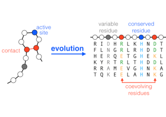
Figure 1: Evolutionary constraints shaping the variability between homologous sequences: While constraints on individual residues (e.g., active sites) lead to variable levels of amino-acid conservation, the conservation of contacts leads to the coevolution of structurally neighboring residues and therefore to correlations between columns in a multiple-sequence alignment of homologous proteins (here an artificial alignemt is shown for illustration).

Coevolution becomes visible in correlated occurrences of amino acids in different sites, i.e. via covariation between different columns of the underlying multiple-sequence alignment (cf. Fig. 1) Göbel et al. (1994); Neher (1994). It is tempting to use such correlations to reconstruct the contact map of a protein, which could then be used to predict the protein fold as a three-dimensional embedding of this contact map. This idea, present in the literature for more than 20 years Göbel et al. (1994); Neher (1994), did unfortunately not work out easily. A major reason is that correlation (as detected in the MSA) is not coupling (as resulting from amino acids in contact): if, e.g., position $i$ is in contact with position $j$, and position $j$ in contact with position $k$, we might expect an indirect correlation also between $i$ and $k$. The aim of the Direct-Coupling Analysis Weigt et al. (2009); Morcos et al. (2011), and of closely related approaches Burger and Van Nimwegen (2010); Balakrishnan et al. (2011); Jones et al. (2012), is to explain correlations via a network of direct coevolutionary couplings, or more precisely, via a generalized Potts model

$${\cal H}(a_{1},...,a_{L})=-\sum_{1\leq i<j\leq L}J_{ij}(a_{i},a_{j})-\sum_{i=1}^{L}h_{i}(a_{i})$$ (3)

containing both local fields $h_{i}$ and pairwise couplings $J_{ij}$.

As will be shown below, the strongest pairwise couplings provide accurate predictions of contacts between residues. This enables protein-structure prediction without the detailed biophysical modeling mentioned before Schug et al. (2009); Marks et al. (2011); Hopf et al. (2012); Nugent and Jones (2012); Sułkowska et al. (2012); Ovchinnikov et al. (2017). The inference of the couplings is, however, a computationally hard task, since the exact calculation of thermodynamic averages (which have to coincide with empirical ones) requires a sum over the exponentially large sequence space (in a disordered model lacking a priori any symmetry). However, any method reproducing the topology of the coevolutionary network underlying Eq. (3), i.e. identifying the strongly pairs, is equally valid for predicting the contact map.

3) Inference of mutational landscapes and quantitative sequence models: Quantifying the effect of mutations is a task of outstanding biomedical importance and can be used as a technique for identifying causative mutations in genetic disease or cancer, or adaptive mutations leading to therapeutic drug resistance. In a general mathematical setting, mutational effects can be described by a mutational landscape, or genotype-phenotype mapping, which associates a quantitative phenotype $\Phi(a_{1},...,a_{L})$ to each amino-acid sequence $(a_{1},...,a_{L})$ de Visser and Krug (2014). Multiple-protein alignments (of patient derived sequences or of homologous protein families) have been used to infer such landscapes from the empirically observed sequence variability Mann et al. (2014); Morcos et al. (2014); Figliuzzi et al. (2016); Hopf et al. (2017); Feinauer and Weigt (2017), using in particular the analytical form of the Potts model Eq. (3). In this context, the couplings $J_{ij}(a_{i},a_{j})$ represent so-called epistatic couplings between mutations.

To quantify the effect of the mutation from amino acid $a_{i}$ to $b$ in position $i$, we can calculate the energy difference

$$\Delta E(a_{i}\to b) = {\cal H}(a_{1},...,a_{i-1},b,a_{i+1},...,a_{L})$$

$$-{\cal H}(a_{1},...,a_{i-1},a_{i},a_{i+1},...,a_{L})$$

between the mutated and the unmutated sequences. Decreasing energies can be interpretated as potentially beneficial mutations, increasing energies as potentially deleterious mutations. Contrary to residue-residue contact predictions inferring the topology of the coevolutionary network is not sufficient any more. We need a quantitative inference of the local fields and couplings, and expect a – possibly non-linear – correlation between energy differences and mutational effects.

4) Protein design and generative sequence models: In a seminal work, Ranganathan and coworkers Russ et al. (2005); Socolich et al. (2005) suggested that the pattern of pairwise residue covariation is actually sufficient to generate artificial but fully functional protein sequences. The basic idea was to shuffle an MSA via a Monte Carlo procedure such that the statistics of single columns (residue conservation) and column pairs (coevolution) remains close to unchanged. In experimental tests, the authors found a substantial fraction of functional non-natural proteins, whereas imposing only the single-column statistics resulted in non-functional amino-acid sequences.

In the context of the modeling proposed here, we speculate therefore that the generalized Potts model Eq. (3) is sufficient to design artificial proteins by Monte Carlo sampling, while the profile model Eq. (2) is not. For this to be true, the inferred model needs to be generative. This means that the model must not only reproduce perfectly the empirical single- and pair-column statistics (within the possibilities of the fitting algorithm), but should generate sequences that are indistinguishable from the natural sequences also in higher-order characteristics, which are not explicitly fitted using Eq. (3). The abovementioned results Russ et al. (2005); Socolich et al. (2005) suggest that this can be actually achieved using models including only local fields and pairwise couplings, while fields on their own are insufficient.

II Statistical Physics of the Inverse Potts Problem

We start from data given as a multiple-sequence alignment $A=\{a_{i}^{\mu}|i=1,...,L,\mu=1,...,M\}$, which contains $M$ sequences of aligned length $L$. We model the statistical variability in these data using generalized Potts models defined in Eqs. (2) or (3). In this section we will provide some background on the underlying inference methodology that connects data and model, in particular on how to infer the model parameters (local fields $h_{i}(a)$ and couplings $J_{ij}(a,b)$).

This methodology will allow us to infer a specific model for each family of homologous proteins. The corresponding MSA are freely available in public data bases, such as Pfam Finn et al. (2016).

II.1 From Data to Empirical Amino-Acid Frequencies

The statistical modeling of protein sequences relies on the fitting of the empirical low-order statistics of the MSA $A$, where each row is a protein sequence, and each column a specific aligned residue position in the proteins. In particular we estimate the frequencies of the occurrence of single amino acids $a$ in the MSA column $i$, and of the co-occurrence of amino acids $a$ and $b$ in columns $i$ and $j$ inside the same protein:

$$f_{i}(a) = \frac{1}{M_{eff}}\sum_{m=1}^{M}\,w_{m}\,\delta_{a,a_{i}^{m}}\ ,$$ (5)

$$f_{i,j}(a,b) = \frac{1}{M_{eff}}\sum_{m=1}^{M}\,w_{m}\,\delta_{a,a_{i}^{m}}\,\delta_{b,a_{j}^{m}}\ ,$$

with $\delta_{a,b}=1$ being the Kronecker symbol, which equals one if amino acids $a$ and $b$ are equal, and zero otherwise.

Note that in the sum we have introduced a sequence-specific weight $w_{m}$, as well as the effective sequence number $M_{eff}=\sum_{m}w_{m}$ Morcos et al. (2011). The reason is that sequences in an MSA cannot be considered as independent configurations drawn from the statistical model $P$. The MSA collects homologous sequences that have a common ancestry. This ancestry is often relatively recent, and as a consequence sequences can be atypically similar to each other because there was no time for them to evolve further apart. While this similarity can be used to reconstruct the evolutionary history (i.e. the phylogenetic tree) of these sequences Felsenstein (2004), in terms of probabilistic modeling it is a sampling bias introducing correlations not related to the structure and function of the proteins. A further bias results from the uneven selection of sequenced species – species close to model species or important pathogens tend to be more frequently sequenced than species without any direct scientific or biomedical interest.

While a proper removal of this bias remains an important open question, it can be counterbalanced by reducing the weight $w_{m}$ of similar sequences in the empirical frequency counts in Eq. (5). In a commonly used definition of the weights in the context of residue-contact prediction, $w_{m}$ equals to the inverse of the number of sequences ${\bf a}^{\ell}$ of Hamming distance $d_{H}({\bf a}^{\ell},{\bf a}^{m})$ (number of positions with distinct amino acids) smaller than $xL$. It has been shown that $x\simeq 0.2-0.3$ leads to accurate and robust results. Note that $\ell=m$ has to be counted, too, so the weight for an isolated sequence is $w_{m}=1$, while it is smaller for any close-to-repeated sequence Morcos et al. (2011).

The empirical frequencies of Eqs. (5) allow for quantifying the level of correlation between the amino-acid occupancies of any pair of positions $(i,j)$. The mutual information

$$MI_{ij}=\sum_{a,b}f_{ij}(a,b)\log\frac{f_{ij}(a,b)}{f_{i}(a)f_{j}(b)}\ .$$ (6)

is zero if and only if sites $i$ and $j$ are statistically independent, and positive else. It might be tempting to use the mutual information as a simple proxy for pairwise couplings. However, in the context of proteins this leads to inaccurate results since correlations emerge from networks of couplings. Inverse methods are needed to disentangle direct couplings from indirect correlations.

II.2 From Amino-Acid Frequencies to Potts models

After extracting the empirical statistics from the MSA we can use it to estimate the parameters of the Potts model. This means enforcing the model to reproduce the relevant empirical statistics, which can be only the first-order statistics given by the $f_{i}(a)$ in the independent-site case or the second-order statistics given by the $f_{ij}(a,b)$ in the case of a pairwise Potts model. The latter constraints lead to a model with pairwise couplings $J_{ij}(a,b)$. This is expected to be more realistic, but comes at a high computational cost since exact inference requires the calculation of thermodynamic averages and thus the partition function ${\cal Z}$ as a sum over an exponential number $q^{L}$ of amino-acid sequences ${\bf a}=(a_{1},...,a_{L})$. In this subsection we will ignore this technical difficulty, discussing the general setting of inverse Potts models. We leave the question of efficient approximations to the next subsection.

II.2.1 The independent-site case (IND)

In the profile case of Eq. (2), all positions in the model distribution $P$ are independent from each other and the joint probability is factorized over positions. We can therefore easily fit the fields $h_{i}(a)$ to satisfy

$$f_{i}(a)=\frac{e^{h_{i}(a)}}{\sum_{b}e^{h_{i}(b)}}$$ (7)

for all positions $i=1,...,L$ and all amino acids $a$. This equation can be, up to a constant, easily inverted through $h_{i}(a)=\ln f_{i}(a)+const$. To avoid fields to become (minus) infinite in the case of unobserved amino acids, a regularization or a pseudocount can be introduced, see below. This model will not reproduce the second-order statistics $f_{ij}(a,b)$ and the probability of co-occurrence of amino acids $a$ and $b$ in the positions $i$ and $j$ is equal to $f_{i}(a)f_{j}(b)$ in the model distribution.

II.2.2 Inference of pairwise Potts models

The parameters of the pairwise model Eq. (3), the local fields $h_{i}(a)$ and the couplings $\{J_{i,j}(a,b)\}$, have to be inferred in such a way that first and second moments of the Boltzmann distribution $P$ correspond to the empirical frequencies. The following equations have to be satisfied,

$$f_{i}(a) = \langle\delta_{a,a_{i}}\rangle_{P}$$ (8)

$$f_{i,j}(a,b) = \langle\delta_{a_{i},a}\delta_{a_{j},b}\rangle_{P}$$

for all $i,j,a,b$. This ensures that the marginal single- and two-site frequencies of the Potts model are equal to the empirical frequency counts derived from the original data set. In this equation, $\langle\cdot\rangle_{P}$ denotes the average over the Boltzmann distribution $P$ in Eq. (1):

$$\langle{\cal O}({\bf a})\rangle_{P}\equiv\sum_{\bf a}\,P({\bf a})\,{\cal O}({\bf a})$$ (9)

for any observable ${\cal O}({\bf a})$ depending on the amino-acid sequence ${\bf a}=(a_{1},...,a_{L})$. The $N_{p}=Lq+\frac{L(L-1)}{2}q^{2}$ equations in Eqs. (8) are coupled and have to be solved simultaneously.

II.2.3 Overparametrization and gauge invariance

Note that Eqs. (8) are not independent. As each site $i$ carries one amino acid $a$, the frequencies $f_{i}(a)$ sum up to one. Hence there are only $L(q-1)$ independent one-point frequencies. Similarly, for each one of the $\frac{L(L-1)}{2}$ pairs $i,j$, only $(q-1)^{2}$ pairwise frequencies $f_{ij}(a,b)$ are independent, as marginalizing over $b$ allows us to recover the single-site frequencies: $\sum_{b}f_{ij}(a,b)=f_{i}(a)$. The number of independent constraints coming from Eqs. (8) is therefore only $N_{c}=L(q-1)+\frac{L(L-1)}{2}(q-1)^{2}$.

The number of parameters, $h_{i}(a)$ and $J_{ij}(a,b)$, defining Hamiltonian ${\cal H}$ in Eq. (3) equals $N_{p}$ and, therefore, exceeds the number of independent equations in Eq.  (8). This overparametrization gives rise to the following gauge invariance: The probability $P({\bf a})$ remains unchanged under the (gauge) transformation

$$J_{ij}(a,b) \leftarrow J_{ij}(a,b)+K_{ij}(a)+K_{ji}(b)\ ,$$ (10)

$$h_{i}(a) \leftarrow h_{i}(a)+g_{i}-\sum_{j(\neq i)}\big{(}K_{ij}(a)+K_{ji}(a)\big{)}\ .$$

Here, $K_{ij}(a)$ and $g_{i}$ are arbitrary quantities. Note that $K_{ij}(a)$ and $K_{ji}(b)$ are not independent since any $(ij)$-dependent quantity added to the first and subtracted from the second leaves the transformation invariant. The total number of independent parameters defining the above transformation equals therefore $N_{q}=L+\frac{L(L-1)}{2}\times(2q-1)$.

Since each gauge transformation leaves the Boltzmann distribution $P$ unchanged, the number of parameters to be fitted to the empirical data actually reduces to $N_{p}-N_{q}$. This equals the number $N_{c}$ of independent equations in Eqs. (8), and the inference problem is well defined once the gauge is fixed. Two widely used gauges are:

• The lattice-gas gauge, in which $h_{i}(q)=J_{ij}(a,q)=J_{ij}(q,a)=0$ for all $i,j,a$, measures all energies with respect to the “empty” configuration $(q,...,q)$, and considers $q-1$ different “particle” types $a=1,...,q-1$.

• The zero-sum gauge (or Ising gauge) assumes that $\sum_{a}h_{i}(a)=\sum_{a}J_{ij}(a,b)=0$ for all $i,j,b$. This gauge generalizes the well-known case of Ising models ($J_{ij}(s_{i},s_{j})=J_{ij}s_{i}s_{j},h_{i}(s_{i})=h_{i}s_{i},s_{i,j}=\pm 1$) to $q$-state Potts spins. Contrary to the lattice-gas gauge above, this gauge does not arbitrarily break the symmetry between the $q$ states of the Potts variables.

As is the case with standard Ising and lattice-gas models, the two formulations are related through a simple (gauge) transformation of the underlying local variables, and are therefore equivalent.

II.2.4 Cross-entropy minimization and Bayesian interpretation

In this section we rewrite the inverse problem in Eqs. (8) in a simpler and more interpretable way. We introduce the cross entropy

$$S_{c}(\{h,J\}) = -\frac{1}{M_{eff}}\sum_{m}w_{m}\,\log P(a_{1}^{m},a_{2}^{m},...,a_{L}^{m})$$ (11)

$$= \log{\cal Z}-\sum_{i,a}h_{i}(a)\;f_{i}(a)$$

$$-\sum_{i<j,a,b}J_{ij}(a,b)\,f_{ij}(a,b)\ .$$

This quantity gives – up to an additive $P$-independent constant equal to the entropy of the empirical distribution $f(a_{1},...,a_{L})=\sum_{m}w_{m}\prod_{i}\delta_{a_{i},a_{i}^{m}}$ of the sequences in the MSA – the Kullback-Leibler (KL) divergence

$$D_{KL}(f||P)=\sum_{\bf a}f({\bf a})\log\frac{f({\bf a})}{P({\bf a})}$$ (12)

between the empirical distribution $f$ (of which $f_{i}(a)$ and $f_{ij}(a,b)$ are marginals) and the Boltzmann distribution $P$. Within the class of pairwise Potts models defined by Eq. (3), a possible parameter choice is the one minimizing $D_{KL}$ and, hence, the cross entropy $S_{c}$. It is easy to check that the minimization with respect to fields $h_{i}(a)$ and couplings $J_{ij}(a,b)$ leads back to Eqs. (8). Note that the Hessian matrix of $S_{c}$ is nonnegative. Zero eigenvalues correspond to directions in which the cross entropy has a minimum for parameters going to (minus) infinity; they make regularization necessary as explained in the next section.

After minimization, the cross entropy $S_{c}$ becomes a function of the empirical one- and two-point amino-acid frequencies; more precisely it is the Legendre transform of the negative free energy $\log{\cal Z}$. The Potts parameters (fields, couplings) act as conjugated parameters to observables (one- and two-point frequencies), in the same way as pressure or chemical potential are conjugated to volume and number of particles in thermodynamical statistical ensembles. One of the basic properties of Legendre transforms is that the derivative of the potential with respect to its control parameters leads to the conjugate parameters.

Minimizing of the cross entropy is equivalent to maximizing the log-likelihood in a Bayesian framework. Bayes’ theorem in fact allows one to express the posterior probability of the model parameters given the data, $P(\{h,J\}|\{{\bf a^{m}}\})$, starting from the probability of the data given the model, $P(\{{\bf a^{m}}\}|\{h,J\})$:

$$P(\{h,J\}|\{{\bf a^{m}}\})=\frac{P(\{{\bf a^{m}}\}|\{h,J\})\;P_{0}\left(\{h,J\}\right)}{P(\{{\bf a^{m}}\})}\ ,$$ (13)

where $P_{0}$ is a prior distribution over the Potts model parameters. When the prior is uniform and the sequences are independently drawn from $P$, maximizing the posterior distribution over all couplings and fields is equivalent to minimizing the cross entropy $S_{c}$ with uniform weights $w_{m}=\frac{1}{M}$. In the presence of a non-uniform prior a term $-\log P_{0}(\{h,J\})$ is added to the cross entropy, which plays the role of a regularization for the Potts parameters. In the example of a Gaussian prior $P_{0}$, this penalty term is equivalent to a $L_{2}$ regularization, cf. next subsection.

II.2.5 Regularization

Typical proteins (or protein domains, which constitute the alignable modules making a protein) have a length of $L\simeq 50-500$. This leads to $N_{c}\simeq 5\cdot 10^{5}-5\cdot 10^{7}$ parameters to be inferred. Combined with limited sampling ($M\simeq 10^{2}-10^{5}$ for typical MSA), this large number of parameters makes regularization to avoid overfitting necessary.

Consider as an illustration the case of two amino acids, $a$ and $b$, that are rarely encountered on their respective sites $i$ and $j$. Assuming their frequencies to be $f_{i}(a)=f_{j}(b)=0.01$ (note that the average frequency of amino acids is $1/q\simeq 0.048$) and that they evolve independently from each other, the probability of finding both amino acids in a sequence is equal to $0.0001$. For MSAs with less than 10,000 sequences, such a sequence is typically not encountered. This results in an apparent anticorrelation, and ultimately, an infinitely negative coupling between the two sites and amino acids. On the contrary, if the combination is found in a single out of much less than 10,000 sequences, it will lead to a large positive but statistically unsupported coupling.

To avoid such sampling effects, various regularization schemes can be used. In practice, a penalty $\Delta S_{c}(\{h,J\})$ is added to the cross entropy (11) during the minimization of the parameters $\{h,J\}$. Standard examples are the $L_{1}$ norm, where

$$\Delta S_{c}^{L_{1}}(\{h,J\})=\gamma_{1}\sum_{i,a}|h_{i}(a)|+\gamma_{2}\sum_{i<j,a,b}|J_{ij}(a,b)|\ .$$ (14)

The non-analyticity in zero penalizes small fields and couplings, forcing them to become exactly zero in value and thus favors sparse networks to be inferred. The $L_{2}$ norm,

$$\Delta S_{c}^{L_{2}}(\{h,J\})=\gamma_{1}\sum_{i,a}h_{i}(a)^{2}+\gamma_{2}\sum_{i<j,a,b}J_{ij}(a,b)^{2}\ ,$$ (15)

penalizes large absolute values of parameters. This is found to be efficient in the context of protein MSA since it removes the spuriously large parameter values based on insufficient sampling.

Another frequently used procedure to limit undersampling effects consists of adding a pseudocount to the empirical one- and two-point frequencies (justifiable via a Dirichlet prior on frequency counts):

$$f_{i}(a) \leftarrow (1-\alpha)\,f_{i}(a)+\frac{\alpha}{q}\ ,$$

$$f_{ij}(a,b) \leftarrow (1-\alpha)\,f_{ij}(a,b)+\frac{\alpha}{q^{2}}.$$ (16)

The introduction of a pseudocount is – up to finite-sample effects – equivalent to assuming that the MSA is extended with a fraction $\alpha/(1-\alpha)$ of sequences with amino acids sampled uniformly. Regularization parameters $\gamma_{1},\gamma_{2}$ and $\alpha$ should in principal vanish as the number of data increases; values for these parameters used in practice will be discussed later on. An alternative way to regularize the inference problem is to reduce the number of Potts states and keep well sampled amino acids only, for example with frequencies larger than some threshold values. The number of Potts states then depends on the site. This can drastically reduce the number of parameters to infer, and a weaker regularization on the remaining parameters can be used.

II.3 Methods of Approximate Inference

The convexity of the properly regularized cross entropy guarantees the uniqueness of the minimum and the optimal parameter values ${h,J}$. This minimum can be found by local convex optimization techniques. A problem is that calculating the averages in Eqs. (8) exactly requires the calculation of the partition function ${\cal Z}$. This is in practice intractable for proteins with hundreds of residues since it includes a sum over all $q^{N}$ sequences. We therefore resort to approximation schemes to solve the inference problem Roudi et al. (2009); Sessak and Monasson (2009); Mézard and Mora (2009); Cocco et al. (2011); Cocco and Monasson (2011); Aurell and Ekeberg (2012); Nguyen and Berg (2012a, b); Decelle and Ricci-Tersenghi (2014). Their relative advantages and disadvantages in the context of protein sequences will be discussed in the Results section.

II.3.1 Boltzmann Machine Learning (BM)

The most straightforward approximation to solve Eqs. (8) is called Boltzmann machine learning Ackley et al. (1985). Starting from an initial guess for the values of the couplings and fields (e.g., the solution of the independent-site model described above), the one- and two-point marginals of $P$ are estimated by Monte Carlo Markov Chain (MCMC) sampling. They are then compared with the empirical one- and two-point frequencies, and the fields and couplings are modified according to

$$h_{i}(a) \leftarrow h_{i}(a)+\epsilon\big{(}f_{i}(a)-\langle\delta_{a_{i},a}\rangle_{P}\big{)}\ ,$$ (17)

$$J_{ij}(a,b) \leftarrow J_{ij}(a,b)+\epsilon\big{(}f_{ij}(a,b)-\langle\delta_{a_{i},a}\,\delta_{a_{j},b}\rangle_{P}\big{)}\ ,$$

where $\epsilon$ is a small parameter. The direction of the update follows the gradient of the cross entropy $S_{c}$. In the case of sufficiently precise MCMC sampling and a sufficiently small $\epsilon$, this iterative procedure is guaranteed to converge towards the solution of the fixed-point equations (8).

This procedure cannot be used directly due to its high computational cost. Efficient implementation going beyond simple gradient descent makes Boltzmann machine learning applicable to protein families smaller than about $L=200$ Sutto et al. (2015); Haldane et al. (2016); Barrat-Charlaix et al. (2016). Large-scale studies for hundreds or even thousands of protein families remains therefore out of reach.

II.3.2 Gaussian Approximation

Using the lattice-gas gauge mentioned before, we can represent each Potts variable $a$ by a $(q-1)$-dimensional vector $(s^{1},...,s^{q-1})$ with entries $s^{b}(a)=\delta_{b,a}$. Amino acids $a=1,...,q-1$ are thus represented by unit vectors in direction $a$, while the reference amino acid (or the gap) is represented by the zero vetor $(0,...,0)$. The MSA becomes a matrix of $M$ rows and $(q-1)L$ columns with binary entries $\{0,1\}$. The average of the column corresponding to position $i$, amino acid $a$ equals the empirical frequency $f_{i}(a)$, the $(q-1)L$-dimensional covariance matrix $C_{ij}(a,b)=f_{ij}(a,b)-f_{i}(a)f_{j}(b),i,j=1,...,L,a,b=1,...,(q-1)$.

The Gaussian approximation ignores the binary nature of the $s$-variables and treats them as continuous variables having the same means and covariances Jones et al. (2012); Baldassi et al. (2014). The pairwise Potts model is transferred into a multivariate Gaussian model with parameters $J_{ij}(a,b)$. The cross-entropy can be calculated analytically (up to a coupling-independent normalization),

$$S_{c}^{G}=-\frac{1}{2}\log\text{Det}{(-J)}-{\sum_{i<j,a,b}}J_{ij}(a,b)\;C_{ij}(a,b)\ .$$ (18)

Eq. (18) can be easily minimized over $J$, giving

$$J_{ij}(a,b)=-\left(C^{-1}\right)_{ij}(a,b)\ .$$ (19)

The original exponential-time inference problem (time $~{}q^{L}$) is replaced by a simple inversion of the empirical covariance matrix, a task requiring $\sim L^{3}$ operations. It can be achieved on a standard desktop computer even for long proteins of $L\simeq 1000$ amino acids.

II.3.3 Mean-field Approximation (MF)

The standard MF approximation allows one to estimate one-point marginals self-consistently. Plugging in Eqs. (8), which equate empirical and model derived frequencies, we find

$$\frac{f_{i}(a)}{f_{i}(q)}=\exp\left\{h_{i}(a)+\sum_{j,b}J_{ij}(a,b)f_{j}(b)\right\}$$ (20)

within the lattice-gas gauge. Covariances can be calculated using linear response, i.e., $\partial P_{i}(a)/\partial h_{j}(b)=C_{ij}(a,b)$. This again leads to Eq. (19) and the couplings can be obtained by inverting the covariance matrix Roudi et al. (2009); Morcos et al. (2011). The fields can then be obtained by resolving Eqs. (20) with given single-site frequencies and couplings.

Together with the Gaussian approximation, MF is currently the computationally most efficient approximative inference scheme for the inverse Potts problem. However, it will not converge to the exact solution even with infinite data, and no rigorous bounds on inference errors are known. One can also formulate refined mean-field approximations, based on e.g., the Thouless-Anderson-Palmer or Bethe-Peierls approximations, but they have not found to be of advantage when applied to protein MSAs.

II.3.4 Pseudolikelihood Maximization (PLM)

In the PLM technique Ravikumar et al. (2010); Aurell and Ekeberg (2012); Ekeberg et al. (2013), the log probability of the data given the parameters in Eq. (11) is replaced by a sum of site-dependent terms:

$$\sum\limits_{m=1}^{M}w_{m}\log P(a_{1}^{m},...,a_{L}^{m})\rightarrow\sum\limits_{i=1}^{L}\sum\limits_{m=1}^{M}w_{m}\log P(a_{i}^{m}|{\bf a}_{-i}^{m})$$ (21)

Here, $i$ denotes a site and ${\bf a}_{-i}$ denotes the sequence $a$ without the $i$th site. Note that the sum contains one term for each $i$ and these terms contain probability distributions over a single amino acid (given the others). This means that for normalizing these terms we need to calculate $L$ individual sums over $q$ amino acids instead of one sum over $q^{L}$ sequences. Setting

$$S_{c}^{PLM}(i)=-\sum\limits_{m=1}^{M}w_{m}\log P(a_{i}^{m}|{\bf a}_{-i}^{m}),$$ (22)

the cross entropy is the sum

$$S_{c}^{PLM}=\sum_{i=1}^{L}S_{c}^{PLM}(i)$$ (23)

over the site-dependent terms. In terms of couplings and fields these terms can be written as

$$S_{c}^{PLM}(i) = \sum_{m=1}^{M}w_{m}\left[\log\left\{\sum_{a}e^{h_{i}(a)+\sum_{j(\neq i)}J_{ij}(a,a_{j}^{m})}\right\}\right.$$ (24)

$$-h_{i}(a_{i}^{m})-\left.\sum_{j(\neq i)}J_{ij}(a_{i}^{m},a_{j}^{m})\right]\ .$$

While $S_{c}^{PLM}$ is not an approximation for the cross-entropy $S_{c}$, the method of minimizing $S_{c}^{PLM}$ can be shown to be statistically consistent Ravikumar et al. (2010): The true couplings and fields are recovered in the limit of infinite data if the data are indeed sampled from a pairwise Boltzmann distribution.

Interestingly, this statistical consistency remains valid if the $S_{c}^{PLM}(i)$ are minimized independently. While this allows for a parallel and efficient implementation, it leads for finite data to asymmetric couplings $J_{ij}(a,b)\neq J_{ji}(b,a)$. In practice, we infer each coupling as the mean of the asymmetric estimates $[J_{ij}(a,b)+J_{ji}(b,a)]/2$.

The key advantage of PLM is that the cross entropy is calculated from the sampled sequences, and there is therefore no need for an exponential-time calculation of the partition function. However, $S_{c}^{PLM}$ does not depend only on the empirical single- and two-site frequencies, but on the complete set of sampled configurations. PLM becomes therefore slower for larger samples and the running time grows linearly with the number $M$ of sequences.

II.3.5 Adaptive Cluster Expansion (ACE)

The minimal cross entropy $S_{c}$ can be formally written as a sum of $2^{L}-1$ cluster contributions Cocco and Monasson (2011), each depending only on the empirical frequencies $f_{i}$ and $f_{ij}$ of the sites inside the cluster:

$$S_{c}^{ACE} = \sum_{i}\Delta S_{i}(f_{i})+\sum_{i<j}\Delta S_{ij}(f_{i},f_{j},f_{ij})$$

$$+ \sum_{i<j<k}\Delta S_{ijk}(f_{i},f_{j},f_{k},f_{ij},f_{jk},f_{ik})+\ldots$$

Here, $\Delta S$ denotes the contribution to the cross entropy from a cluster that cannot be deduced from the contributions of all its subclusters Cocco and Monasson (2012). Expansion (II.3.5) is, however, of limited use if not truncated to a small number (compared to $2^{L}$) of terms. A convenient truncation scheme is obtained by summing only contributions $\Delta S$ exceeding (in absolute value) an arbitrary threshold $\theta$, as large cluster contributions automatically identify groups of strongly interacting variables. In practice, clusters are recursively constructed, starting from small size ones (2 sites) through progressive inclusion of sites. The process is iterated until all newly created clusters have $|\Delta S|$ smaller than $\theta$. The derivatives of $S_{c}^{ACE}$ with respect to the frequencies $\{f_{i}(a),f_{ij}(a,b)\}$ give access to the Potts parameters $\{h_{i}(a),J_{ij}(a,b)\}$. The threshold $\theta$ is tuned such that the inferred model reproduces the data statistics, as can be verified through Monte Carlo sampling, up to finite-sampling errors.

ACE, similarly to Boltzmann-machine learning and differently from the Gaussian, mean-field and pseudolikelihood approximations, accurately reproduces the sampled frequencies and correlations by construction Cocco and Monasson (2012); Barton et al. (2016a). Due to the properties of the inverse susceptibility (Fisher information) matrix, the convergence of the expansion depends on the structure of the interaction graph rather than on the magnitude of data correlation. The threshold $\theta$ acts as a regularizer: the complexity of the network is adapted to the level of sampling, in particular it will be sparse for bad sampling. The disadvantage of ACE is that it is computationally more involved than any of the other approximative methods: it requires the exact calculation of the partition function for each cluster. The computational burden is largely decreased by the compression of the number of Potts states to restrict the inferred model to only well observed amino acids, as described above, and by the possibility to run it in combination with Boltzmann-machine learning Barton et al. (2016a).

II.3.6 Other Approaches

There are several other interesting methods, e.g. minimal probability flow Sohl-Dickstein et al. (2011) or Bayesian networks Burger and Van Nimwegen (2010), which have been applied to protein sequence modelling.

III Modeling Families of Protein Sequences

After having adressed inverse models in statistical physics from the methodological point of view, we will give a few exemplary results from using these methodologies with real protein sequence data.

III.1 Homologous Protein Families and Profile Models

State-of-the-art techniques for homology detection and sequence alignments are based on the patterns of amino-acid conservation in individual positions Durbin et al. (1998). A class of statistical models are independent-site profile models, which assume all positions (or columns in an alignment) to be statistically independent. In the case of unaligned sequences, profile models can be generalized to profile hidden Markov models. These combine residue conservation patterns with the possibility of identifying insertions and deletions in a sequence and are among the most successful statistical models in bioinformatical sequence analysis. They are at the basis of databases of homologous protein families such as Pfam. The Pfam database (release 28.0 in 2015) contains 16,230 protein domain families, out of which 6,783 contain more than 1,000 sequences Finn et al. (2016). This number of sequences is empirically known to be a lower bound to the size of an input MSA providing accurate and robust predictions by pairwise statistical modeling. Only 10 years ago, there were about 600 families (release 20.0 in 2006) in Pfam, and the number of accessible families continues to grow quickly. Approaches from inverse statistical physics that go beyond profile models can now be applied to the majority of protein families.

III.2 Potts models: accurate fitting vs. topological inference

The inference of the couplings and fields of a pairwise Potts model (3) from aligned amino-acid sequences is a computationally hard task. It is expected that the approximate inference methods vary in quality of the resulting predictions. Since a “true” model does not exist – evolution is not a Monte Carlo simulation of a Boltzmann distribution – it is not clear how to assess the accuracy of the inferred model. A straight forward benchmark would be to check if Eqs. (8), which equate empirical and model statistics, are well fitted. Using the protein family PF00014 (Trypsin inhibitor: $L=53,M=4915$) as an example, we apply the different approaches discussed in the last section for parameter inference. Subsequently we sample artificial sequences from the inferred statistical model $P(a_{1},...,a_{L})$ using MCMC, in order to estimate the model statistics. In Fig. 2 we show the results: While mean-field inference Morcos et al. (2011) and pseudo-likelihood maximisation Ekeberg et al. (2013) reproduce the empirical statistics badly (mean-field actually leads to serious problems in equilibration MCMC simulations), BM Figliuzzi et al. (2017) and ACE Barton et al. (2016b) are much more precise.

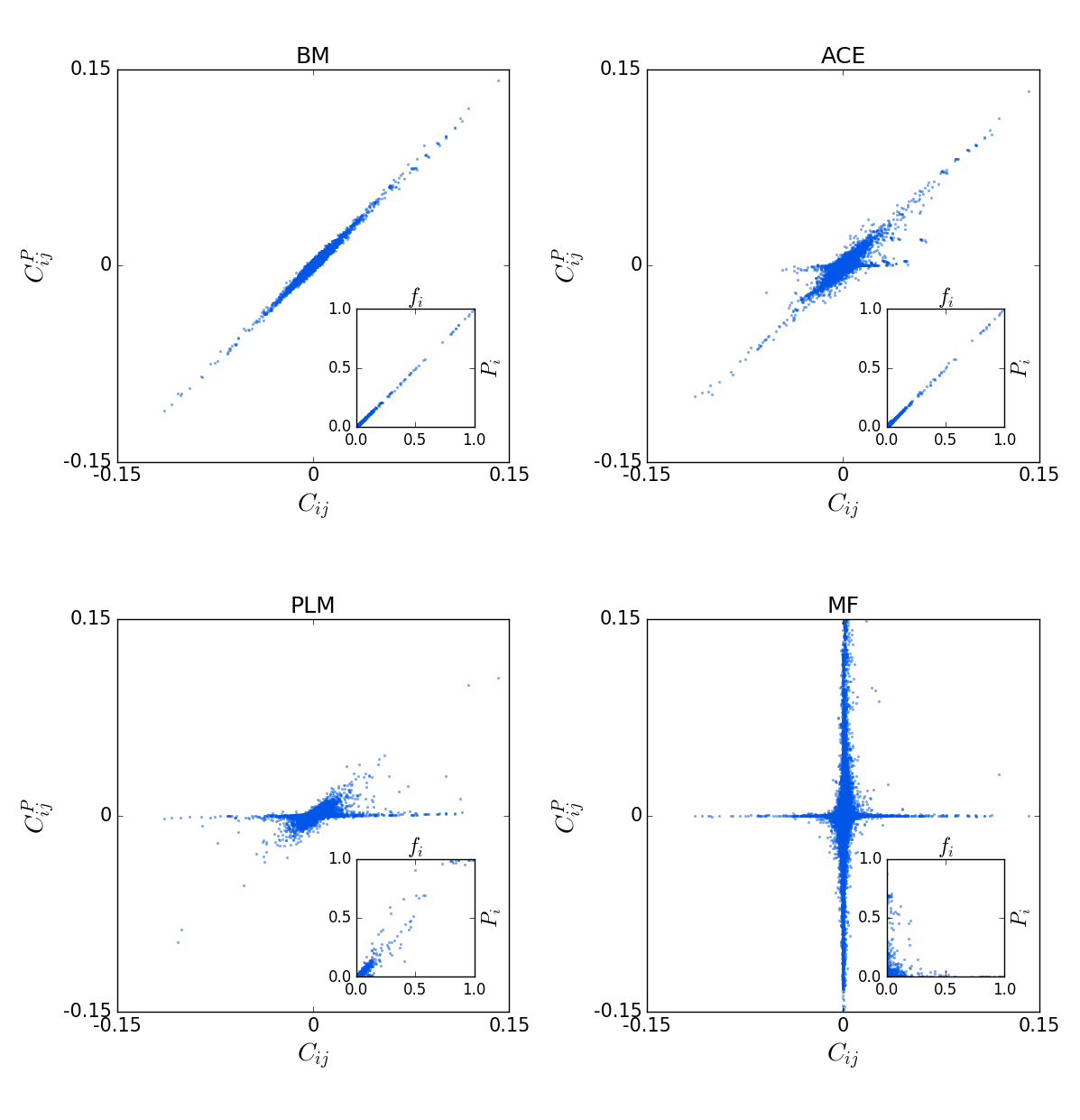
Figure 2: Comparison of different methods: Covariances (main panels) and single-point frequencies of the model P as commpared to the empirical values resulting from the original MSA. While the Boltzmann machine (BM) is guaranteed to accurately fit the empirical values after e sufficient number of iterations of Eq. (17), all others are based on approximations. MF does not reproduce the empirical statistics (it actually has important ergodicity problems when sampling by MCMC), while PLM shows a clear improvement. ACE accurately fits the single-sire frequencies and large enough covariances, deviations for small covariances result from lumping together all symbols $a$ with probabilities $f_{i}(a)<0.05$, such covariances have therefore low statistical support and large relative error, cf. Barton et al. (2016a)).

Does this mean that MF and PLM are of no use for analysing large MSA? As argued in the introduction, the answer is not so easy. When predicting residue contacts in the three-dimensional fold of a protein, we do not need the fine statistics of the empirical data to be reproduced. We need to correctly capture the topology of the network of coevolutionary couplings.

To assess the topology, we need to map the $q\times q$ coupling matrix $J_{ij}(a,b)$ for each pair $(i,j)$ onto a scalar quantity measuring the coupling strength between the two sites $i$ and $j$. A quantity often used Ekeberg et al. (2013) is the Frobenius norm of the coupling matrices for each $(i,j)$,

$$F_{ij}=\sqrt{\sum_{a,b}J_{ij}(a,b)^{2}}\ .$$ (26)

Since the Frobenius Norm is gauge dependent, we have to specify in which gauge we calculate it. A sensible choice is the zero-sum gauge discussed above. It minimises the Frobenius norm and explains thereby “as much as possible” by fields, and “as little as necessary” by pairwise couplings. Contact predictions improve furthermore when using the average-product correction (APC) Dunn et al. (2008):

$$F_{ij}^{APC}=F_{ij}-\frac{\sum_{k}F_{ik}\sum_{k}F_{kj}}{\sum_{k,\ell}F_{k\ell}}\ .$$ (27)

This correction is identical to the measure of modularity commonly used for describing networks Jacquin (2015), and amounts to substracting from the Frobenius norm a null-model contribution for the pair $i,j$ due to the single-site properties of $i$ and $j$ Newman (2006).

The resulting $F^{APC}$-values are highly correlated for different methods. In particular the largest values, which characterize the sub-network of the strongest coevolutionary couplings, are found to strongly overlap. As an example, out of the top 50 coupled pairs found by BM, 80% (resp. 70% / 62%) are also within the first 50 pairs identified by PLM (resp. MF / ACE); these fractions rise to 100% (resp. 88% / 76%) if we look for these 50 top-scoring BM predictions within the first 100 PLM (resp. MF / ACE) pairings. The lower overlap between ACE and the other methods results from the weaker regularization used, which allows for a better fitting but at the cost of introducing a number of strong couplings between rare amino acids. A random selection of 50 pairs for each method would result in an mean overlap of less than 4%, illustrating the high significance of the reported overlaps.

We conclude that if the aim of the inference is the identification of pairs with substantial coevolution, then even simple and computationally efficient methods like MF and PLM can provide accurate results. If, on the contrary, model energies or probabilities have to be accurate, then more precise methods such as ACE or BM are required. This is for example the case if one wants to sample from the inferred distribution.

Another interesting observation is reported in Fig. 3, which shows histograms of Hamming distances of sequences to the consensus sequence $(a_{1}^{\star},...,a_{L}^{\star})$ given by the most frequent amino acids $a_{i}^{\star}={\rm argmax}_{a}f_{i}(a)$ in each column $i$, comparing natural sequences from the original MSA to sequences sampled from different inferred models. While the independent model IND reproduces the average distance (by definition of IND and the linearity of the Hamming distance), the histogram is visibly more concentrated than for natural sequences. PLM shows systematic deviations due to the lack of fitting accuracy, while ACE and BM accurately reproduce the empirical histograms. This is astonishing since the histogram measures quantities which are not fitted via the Potts model, and illustrates the capacity of statistical models with pairwise couplings to well capture the sequence variability even beyond pairwise observables.

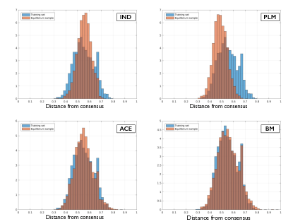
Figure 3: Comparison of different methods: The panels show histograms of Hamming distances of natural and model-generated sequences from the consensus sequence. The blue curves show the histograms for natural sequences (sampled from the initial MSA with frequencies proportional to the sequence weights), the orange ones for the different models (IND, PLM, ACE, BM). While IND and PLM show significant deviations, ACE and BM accurately reproduce the empirical histograms. Note that the measured distance is not fitted by the Potts model and therefore not automatically reproduced even by an accurately inferred Potts model.

III.3 Residue-residue contact prediction and tertiary structure

The original motivation underlying the use of Potts models for describing the sequence variability across evolutionary related proteins is the prediction of residue-residue contacts Weigt et al. (2009). This task is considered hard but important in bioinformatics: Experimental determination of protein structures (X-ray crystallography, NMR, cryo-electron microscopy) is expensive, time consuming, and frequently of uncertain outcome. On the other hand, freely accessible sequence databases are growing fast. If it were possible to use such sequence data for predicting contacts between residues, this information could in turn help to predict protein structures (intra-protein contacts) or to assemble multi-protein complexes (inter-protein contacts). Since protein function typically relies on protein structure (e.g. via binding of other molecules to well defined interfaces on the protein surface), this would provide crucial information about the operation of the proteins and the biological processes they participate in. The validity of contact predictions is assessed by comparison with known structures of proteins belonging to the family under consideration. This structural information is complementary to the sequence data and only available for a fraction of protein families.

Within DCA, residue position pairs $(i,j)$ are sorted according to their interaction strengths as measured by $F_{ij}^{APC}$. We expect the most coupled pairs to be in contact. High scores are thought to indicate compensatory mutations in neighbouring residues in a protein structure (cf. Introduction).

Pairs of residues $i,j$ with short separation $|i-j|$ along the backbone frequently possess large $F_{ij}^{APC}$-values. These large scores often come from the presence of stretches of gaps, and are not very much relevant as far as structural predictions are concerned. For this reasons and since long-range (along the protein backbone) contacts are more informative about the tertiary structure most predictors do not include pairs with $|i-j|\leq 4$ into the evaluation, a distance corresponding to one turn in an $\alpha$-helix.

Fig. 4 shows an example for this procedure. Results obtained for 4,915 sequences of length 53 amino acids, all belonging to the Pfam protein family PF00014 (trypsin inhibitor), are mapped onto the corresponding X-ray crystal structure (PDB ID 5PTI Wlodawer et al. (1984)). The left panel shows that the prediction by the strongest correlations (as measured by mutual information (6)) includes a large fraction of false positives (green lines). Predictions based on the strongest couplings, shown in the right panel, lead to a significantly better prediction (red lines).

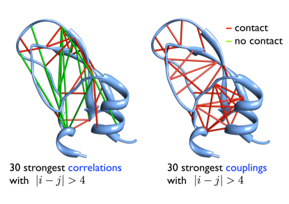
Figure 4: Residue-residue contact prediction based on ranking of correlations (left) and Potts couplings (right) for the PF00014 protein family (trypsin inhibitor). Top 30 values of the mutual information (i.e. correlations) and $F^{APC}$ (i.e. couplings) scores are mapped onto the protein structure (PDB ID: 5PTI), excluding trivial predictions with separation $|i-j|\leq 4$ along the amino-acid sequence. Red bars correspond to residue pairs in contact (distance below 8Å, true positives), green bars to distant residue pairs (false positives). Inference was done using the mean-field approximation.

While here we present only one example, the predictive performance has been tested for thousands of protein families Morcos et al. (2011); Ovchinnikov et al. (2017). A consistent improvement of DCA over correlations has been shown. Interestingly, the quality of the inference has only a small impact on the contact prediction. The reason is that in order to obtain a good performance in contact prediction, it is sufficient to infer the topological aspects of the network reasonably well. While approximate methods like MF or PLM may have a larger error in the inference of the exact parameter values than more exact methods like BM or ACE, they robustly predict network topology, cf. the last section. In fact, PLM is currently the best stand-alone method for efficient contact prediction.

The central use for the residue contacts extracted from MSAs with DCA is in the prediction of protein structures. While the structure of a protein is usually defined by its amino-acid sequence (Anfinsen’s principle Anfinsen and Scheraga (1975)), the general process of protein folding in vivo is not known. Setting this question aside for the moment, one can also ask the easier questions on how to computationally infer the folded structure of a protein from its sequence. In the last decades, this was a central question in computational biology and many methods have been devised. Even though the performance of these methods has made impressive advances, the problem is still considered as unsolved in general Dill and MacCallum (2012).

In this context, DCA has been shown to provide valuable information. The predicted residues can be used as prior information on the structures. Such information restricts the number of possible structures and makes the task thus easier. The importance of predicted contacts in the field can be illustrated by the fact that many of the top-performing groups in the last CASP challenge (http://predictioncenter.org/) have made use of them. Thousands of novel protein structures have been predicted using coevolutionary contact predictions Ovchinnikov et al. (2017).

As a last point, we note that the best performing methods for predicting residue contacts are meta-methods. These methods use other methods like DCA as input and combine them using machine-learning techniques for an improved prediction Skwark et al. (2014); Jones et al. (2015); Wang et al. (2017). Since they use supervised learning techniques to model the input-output relation between MSA and contact map, it is not surprising that they outperform any unsupervised method in this task.

III.4 Predicting interaction partners and inter-protein residue contacts in protein-protein interaction

The formalism of Potts Models and DCA can be used to extract biological information on different scales. While we focused above on how to infer contacts between residues within a protein, we now describe how to use the same formalism to infer interactions between proteins Ovchinnikov et al. (2014); Feinauer et al. (2016). When extended to all proteins in a genome, this can then be used to infer an organism-wide protein-protein interaction network.

The model in Eq. (3) defines a probability $P({\mathbf{a}})$ for finding sequence ${\mathbf{a}}$ for a specific protein belonging to protein family $A$ in an organism. We now define a probability $P({\mathbf{a}},{\mathbf{b}})$ for finding sequence ${\mathbf{a}}$ for a protein belonging to family $A$ and sequence ${\mathbf{b}}$ for a protein belonging to family $B$ in the same organism. The general idea is that if the members of the two protein families interact in all or most organisms, they have to be mutually compatible. Therefore, one would expect $P({\mathbf{a}},{\mathbf{b}})\neq P({\mathbf{a}})P({\mathbf{b}})$ in such cases.

An intuitive extension of Eq. (3) for two protein sequences ${\mathbf{a}}$ and ${\mathbf{b}}$ is

$${\cal H}({\mathbf{a}},{\mathbf{b}})={\cal H}^{A}({\mathbf{a}})+{\cal H}^{B}({\mathbf{b}})+{\cal H}^{AB}({\mathbf{a}},{\mathbf{b}}),$$

where ${\cal H}^{A}({\mathbf{a}})$ and ${\cal H}^{B}({\mathbf{b}})$ are of the form of Eq. (3) and model the coevolution between residues within the proteins $A$ and $B$. The additional interaction term

$${\cal H}^{AB}({\mathbf{a}},{\mathbf{b}})=-\sum\limits_{i=1}^{L_{a}}\sum\limits_{j=1}^{L_{b}}J_{ij}(a_{i},b_{j})$$

contains $L_{a}L_{b}q^{2}$ coupling parameters, with $L_{a}$ and $L_{b}$ being the length of the sequences ${\mathbf{a}}$ and ${\mathbf{b}}$. These parameters describe the coevolution between residue pairs in different proteins.

The model including the interaction term defines a probability for a pair of sequences in the same organism. As data for the inference process we therefore need two MSAs, one for protein family $A$ and one for protein family $B$. We then search for pairs of sequences (one from $A$ and one from $B$) that come from the same organism and treat their concatenation as a single configuration of the composed Potts model.

A problem can arise when there are several sequences belonging to the same protein family inside a single organism (such sequences are called paralogs). The problem which sequences to pair in such cases is called matching and can be solved either by biological prior information Ovchinnikov et al. (2014); Feinauer et al. (2016) or by another layer of probabilistic modeling Gueudré et al. (2016); Bitbol et al. (2016).

As an interaction score for residue pairs between two proteins the $F^{APC}$ scores of Eq. (27) can be used. A possible interaction score for two proteins is then the average of the $n$ largest $F^{APC}$ scores between the proteins. It has been shown that $n=4$ gives a good performance, since it takes into account the strongest signals, but averages over a few pairs to be less susceptible to noise.

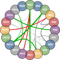
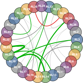
Figure 5: Protein-protein interaction network of the small ribosomal subunit (SRU, top) and the large ribosomal subunit (LRU, bottom). Circles represent proteins, grey and green lines represent interactions found in the experimental structure (PDBs: 2Z4K/2Z4L). The 10 colored lines represent the 10 strongest interaction scores according to DCA. Green indicates a true positive, red a false positive. The width of the lines is proportional to the number of residue contacts between the proteins (figures from Feinauer et al. (2016)).

In Fig. 5 we represent as an example the inference results for the two ribosomal subunits. The units consists of 49 proteins and within the experimentally determined structure (PDB: 2Z4K, 2Z4L Borovinskaya et al. (2007)) 50 pairs are interacting, i.e. only 8.4% out of the 596 intra-unit protein pairs. We use the approach outlined above to fit a Potts Model to each of the corresponding 596 protein-family pairs and calculated interaction scores with $n=4$. Of the ten pairs with the largest interaction scores in each unit, 16 are interacting in the structure, covering most pairs with large interaction interfaces (i.e. fat lines in the figure). This predictive precision of 80% has to be compared with the 8.4% to be expected on average in a random prediction, i.e. only 1.68 interacting pairs would have been found on average when extracting 20 random pairs, with no preference for large interfaces.

Since one Potts Model has to be inferred per protein pair, the method is computationally expensive for large sets of proteins. It has nonetheless been applied to large-scale datasets, such as all protein pairs within an operon (a set of co-localized genes expressed together) in a genome Ovchinnikov et al. (2014).

The same method can also be used to infer residue-residue contacts between proteins. Such predictions are useful when searching for the structure of a protein complex when the structures of the single proteins are known Schug et al. (2009); Dago et al. (2012); Ovchinnikov et al. (2014); Hopf et al. (2014); Uguzzoni et al. (in press 2017). It has been seen that large protein-protein interfaces, which are widely conserved across species, show reliable coevolutionary signals, while smaller interfaces or those being only conserved in part of a protein family cannot be easily detected by a global statistical modeling of a protein family Uguzzoni et al. (in press 2017).

III.5 Potts model for scoring: From single mutations to entire sequences

The Potts model inferred from the MSA of a protein family defines a distribution over all sequences, assigning higher probabilities to sequences likely to belong to this family. It can thus be used to quantitatively predict whether a sequence is similar in structure and function to the sequences the model has been trained on. In this way the model becomes a tool for assessing the effect of mutations in protein sequences, for predicting whether synthetic sequences fold into a known structure or for generating new synthetic sequences by sampling from the model.

A natural quantity to score sequences in these applications is their energy. By definition, Eq. (3) is minus the log-probability of the sequence (up to an additive constant coming from normalization). We now show that this score leads to very promising results when tested on experimental data.

A local test checks if energy differences (i.e. differences in log-probability of the Potts model) actually can quantify the fitness effect of mutations. This has been done successfully in a number of situations, ranging from viral over bacterial to human proteins Mann et al. (2014); Morcos et al. (2014); Figliuzzi et al. (2016); Hopf et al. (2017); Feinauer and Weigt (2017). Such predictions are of great biomedical interest, since they help to find mutations related to virulence or drug resistance of pathogens to the identification of disease-causing mutations in between the multitude of neutral polymorphisms observable in human.

On a more global level, the energy of the Potts model can be seen as a measure in how far a new (e.g. artificially designed) amino-acid sequence is compatible with the natural sequence variability extracted via our Potts model from known sequences (i.e. the MSA used to infer the model parameters). This was first done in Balakrishnan et al. (2011) using PLM-based inference and experimental data from Socolich et al. (2005); Russ et al. (2005). The latter works are based on a method called Statistical Couplings Analysis (SCA), which was used for generating computationally non-natural members of the WW protein domain family (PFAM family PF00397, with an MSA of currently $M=12742$ sequences).

The SCA sampling process is based only on the statistical properties of an MSA of natural members of the family; the resulting non-natural sequences were expressed and tested experimentally. The properties determined were thermodynamic stability in Socolich et al. (2005), and the peptide binding specificity for a subset of stable proteins in Russ et al. (2005).

The starting point for the generation of artifical sequences was a small and curated alignment of 120 natural sequences of the WW domain family (length 35 residues), 42 of which were included in the experiments (called NAT – natural). To generate artificial sequences, the alignment was shuffled in three different ways:

• (R – random): A random permutation was applied to all entries in the matrix, thereby destroying any pattern of site-specific conservation (i.e. “magnetization”) or covariation between sites. 19 sequences were tested experimentally.

• (IC – independent conservation): Sequences were obtained by shuffling each column of the original MSA. Statistical features of individual positions are therefore unchanged, while covariation patterns are destroyed. The IC shuffling procedure corresponds to a sampling from the independent-site model Eq. (2). 43 sequences were tested experimentally.

• (CC – coupled conservation): Starting from the IC data set, a Monte-Carlo annealing was used to to approximately reproduce the pairwise amino acid frequencies $f_{ij}(a,b)$ of the original MSA of natural sequences. The CC dataset is closely related to a sampling from the Potts model in Eq. (3), cf. Bialek and Ranganathan (2007). 43 sequences were tested experimentally.

Denaturation experiments showed that none of the R or IC sequences folded into the correct structure. On the contrary, $31\%$ of the CC sequences and $67\%$ of the NAT sequences folded correctly in the experimental conditions used. These results are a strong indication that limited sequence information might be sufficient for defining the structural constraints acting on the evolution of the WW domain family. Considering the complexity of interactions between amino acids, illustrated by the notorious difficulty of solving the protein folding problem Dill and MacCallum (2012), this may come as a surprise. More exactly, reproducing the pairwise correlations in the amino-acid distribution, in addition to the single-site frequencies, seems to be necessary and (almost) sufficient to specify the native fold.

However, the SCA algorithm was not able to score single sequences, but only the entire shuffled alignement. On the contrary, single sequences can be assessed by the Potts-model energies described before. It was first noted in Balakrishnan et al. (2011), that these energies are effectively an excellent predictor which of the sequences fold, and which not.

Using the couplings $J_{ij}(a,b)$ and fields $h_{i}(a)$ inferred with a recent Pfam release, sequence energies for the different sets were calculated. We compare them to energies of sequences sampled from the same Potts model and the independent model in Fig. 6. In the top panel, the energy distribution of sequences generated from a Monte Carlo sampling of the inferred Potts model (blue) is compared to the distribution of energies of sequences generated by the independent model (green) and from random sequences (red). In the bottom panel, the sequences tested experimentally in Socolich et al. (2005) are shown - by red bars if they were folding in the experiments, by grey bars if not.

As a first observation, we see that also the IC sequences (as well as the sequences sampled from the independent model) have significantly smaller energies than the random sequences, even if these are evaluated with the pairwise Potts model. The energy spectra of the sample from the Potts and the independent model are partially overlapping, resulting also in overlapping energy values of the CC and IC sequences. The most striking observation is, however, that most folding CC and N sequences have energies smaller than those achieved by IC and independent-model sequences, while the CC and N sequences with higher energies, in the range of IC energies, are mostly non folding. The energy turns out to be an excellent discriminator between folding and not folding sequences across the NAT, CC, IC and R data sets.

Fig. 6 shows the results obtained using ACE for model inference. While the other inference techniques (MF, PLM, BM) show some quantitative differences, their performance in discriminating folding from non folding sequences is very comparable: The performance of Potts models in such classification tasks does not depend much on the inference technique used. This is probably due to the fact that the inferred parameters have to be only good enough to rank the sequences correctly, such that a more precise inference does not lead to a better performance in sequence ranking.

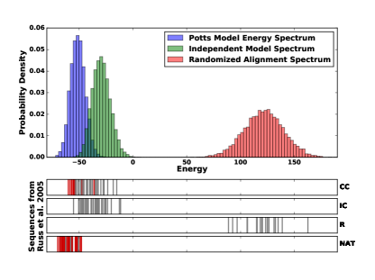
Figure 6: WW sequences: Potts energies and folding qualities. Top: Distribution of Potts energies with couplings and fields parameter inferred by the ACE algorithm sampled by MCMC from the coupled Potts (red) and the Independent-site (green) models. Bottom: First row: Energies of the 43 CC sequences, among which 12 well folded (red) and 31 (gray) not well folded. Second row: Energy of the 43 IC sequences, among which none of them fold. Third rows: Energies of the 42 Natural Sequences, among which 28 well folded (red) and 14 (gray) not well folded according to the denaturation tests. The 19 random sequences have all higher energies ${\cal H}>0$.

III.6 Generative aspects and entropy: from lattice proteins to HIV

An ambitious goal is to generate new and functional protein sequences, e.g. by Monte Carlo sampling from the inferred model, along the lines of the study of the WW domain by Ranganathan and collaborators Socolich et al. (2005); Russ et al. (2005), cf. Fig. 6. The question was also addressed in Jacquin et al. (2016) in the highly idealized case of lattice proteins, a model of 27 amino-acid long chains folding on discrete $3\times 3\times 3$ cubic structures Shakhnovich and Gutin (1990). In this setting, protein families are defined as the set of sequences folding into one of the $\sim 10^{5}$ structures on the cube. Jacquin et al. Jacquin et al. (2016) found that new sequences generated by MCMC from the ACE-inferred Potts model describing a structural family have high probability to fold into the same structure (but not for less precise Potts models based on MF and PLM inference). On the contrary, sequences sampled from the independent model rarely fold. These results confirm – in the simple case of lattice proteins – the claim of Socolich et al. (2005); Russ et al. (2005) that keeping 2-point statistical information is necessary and sufficient for generating structurally valid proteins.

As discussed above, the cross-entropy is an estimate of the Gibbs-Shannon entropy of the sequence distribution of proteins belonging to the same family, based on the limited sample of known functional sequences. Roughly speaking, the entropy can be thought of as the logarithm of the number of sequences in the family. This definition is approximate, as some sequences may express the biological function with varying degrees. Computing the value of the entropy is of interest, since it allows us to quantify the diversity of possible proteins sharing a common biological function. The size of a protein family is expected to be much larger than the size of the available MSA. Considering again lattice proteins on the $3\times 3\times 3$ cube allows one to obtain a quantitative understanding of thses concepts in an idealized case Jacquin et al. (2016). Calculations show that the $\sim 10^{5}$ families defined by the possible structures contain each a variable number of protein sequences. The numbers range between $10^{20}$ and $10^{25}$ Barton et al. (2016c) and depend on the designability of the native fold Li et al. (2002); England and Shakhnovich (2003). The total number of sequences in any of the structures represents thus a tiny fraction of the total number of sequences, $20^{27}\simeq 10^{35}$.

While estimating the entropy of real protein families is a daunting, not well-defined task, approximate results can be obtained from the crossentropy when using ACE to infer Potts models Barton et al. (2016c). For the case of the WW domain discussed before, this amounts to approximately 1.2 nats per residue position, i.e. to about $e^{1.2}\simeq 3.3$ different amino acids per site. As the Potts model takes into account only the one- and two-point statistics, we expect the true entropy, which reflects higher order statistical constraints, to be smaller (note that the independent-site model, which does not take into account pairwise correlations, gives a higher entropy density of about $\ln 5.5\simeq 1.7$ nats). All these estimates are obviously much smaller than the value $\ln 20\simeq 2.99$ nats, which would be obtained for purely random amino-acid sequences. They are closer to the value of $1.9$ nats obtained by Shakhnovich an collaborators from purely thermodynamical considerations Shakhnovich (1998).

The concept of entropy was also recently used in the study of HIV viral sequence variability. HIV is characterized by a large sequence mutability: the viral population constantly escapes from the immune system by mutating amino acids in the epitope, a subsequence of about 10 amino acids, which is recognized by antibodies. Understanding the mutational landscape of HIV sequences is therefore of fundamental importance in the hope to design drugs or vaccines that block as many escape mutations as possible. As compensatory mutations (i.e. epistasis couplings between amino acids, as included in the Potts models of protein sequences) play a central role in the escape mutations, it is important to use predictive models that take into account couplings between amino acids. In the following we illustrate a few studies, allowing to more accurately characterize the mutational landscape.

In Fig. 7, we plot the cross entropies of all the 14 proteins encoded in the HIV virus genome. These quantities allow us to identify the viral proteins that are more conserved and therefore less inclined to mutations Barton et al. (2016c). Interestingly, among the three more conserved proteins, the reverse transcriptase and integrase are not frequently targeted by the immune system, and therefore not under its selective pressure. On the contrary, protein p24, which forms the viral capsid, is frequently targeted by the host immune system. Its large conservation despite this immune pressure suggests that this protein is tightly constrained. Epitopes in this region have been shown to be frequently targeted by individuals that efficiently control the viral infection Dahirel et al. (2011). In addition one can predict to what extent variations in amino acids at individual sites contribute to the total entropy of the protein. Neglecting couplings between sites, this can be easily obtained from data Ferrari et al. (2011) using the single site entropy as estimated from the empirical frequencies of amino acids on the sites, $S_{site}(i)=-\sum_{a}f_{i}(a)\log f_{i}(a)$. Corrections to these estimates can be done once the Potts couplings are inferred, as shown in Barton et al. (2016c).

More results were obtained by applying the Potts approach to HIV sequence data. In Mann et al. (2014), the energy cost of sequence mutations with respect to the wild type sequence has been estimated by the inferred Potts model and compared to in vitro measures of the viral replicative power, which is a direct measure of this fitness. A correlation coefficient of $-0.76$ was observed. In Barton et al. (2016d), data consisting of samples of the viral sequences and antibody populations in the same patients over time have been analyzed and compared to Potts model prediction. It has been shown that two patients, in which the same epitope is targeted in the same protein, have escaping times that are very different. Such observations are explained by the fact that the overall viral sequence is different in the two patients and therefore the cost of the escaping mutations, according to the energy cost estimated by the Potts model, is different due to the coupling terms. The energy cost is therefore a good estimator for the time for the escaping mutations .

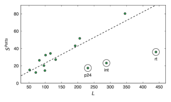
Figure 7: Entropies of the 14 protein families of the HIV virus, as estimated by the ACE algorithm extracted from the alignments (Los Alamos data base), vs. length of the protein. Results are shown for Clade B of the HIV virus, and are similar to what is found for Clade C, see Barton et al. (2016c).

IV Conclusion and outlook

In this review, we have illustrated how methods borrowed from (inverse) statistical physics are gaining influence in the analysis of massive sequence data. Such data become available at an unprecedented pace thanks to next-generation sequencing. The large amounts of data pose both a challenge and an opportunity for sophisticated methods of data analysis and modeling:

• From the point of view of bioinformatics, computational methods are needed to analyse data and gain insight into specific systems of biological and biomedical interest. An example is the use of sequence data to predict the three-dimensional structure of a folded protein.

• From the point of view of statistical biological physics, such large amounts of data help to gain deep insight into general principles governing biological systems and their evolution. As an example, analysing the sequence variability between evolutionary related proteins provides information about how and which structural and functional characteristics of proteins constrain its evolution over millions of years.

Within the statistical modeling of large biological data sets, both viewpoints meet and reinforce each other, placing the area of research at the interface between statistical physics, bioinformatics and biology.

Despite the success of modeling protein sequences via Potts models, there are important limitations, which require substantial theoretical and applied work in the years to come:

• The success of pairwise models is astonishing – there is no fundamental reason why higher-order statistical features (and thus higher-order statistical couplings) should not play a role. It is interesting to unveil the reasons of this success, as well as its limitations. This question is particularly important in the context of the discussed generative models – a true generative model should produce sequences which, by no statistical means, are distinguishable from natural sequences.

• Current modeling schemes assume amino-acid sequences to be configurations of abstract symbols, which have no meaning on their own. Obviously, there is much prior knowledge about amino-acids, there are many methods to predict, e.g., the secondary structure of a protein based on its sequence, the solvent accessibilty of a residue, or the propensity of two residues to form a contact based on their physicochemical properties. So far, such complementary knowledge is not taken into account. As is illustrated by metapredictors using machine-learning techniques for combining coevolutionary scores with prior knowledge, the integration of different data sources is of the utmost importance. Systematic approaches combining heterogenous sources of information in a principled way have to be developped within the statistical-physics community.

• Up to empirical statistical corrections (reweighting), current models assume sequences to be an independently and identically distributed sample drawn from some unknown probability distribution. For sequence data, this assumption is wrong – biological sequences have a non-trivial phylogenetic distribution, and the independent evolution between two recently divided species is typically not “at equilibrium”, i.e. the sequences cary memory about the common ancestor. What is the correct treatment of such sampling biases?

• Last but not least, the methods have been tested in general on sample cases with known answer. Large-scale predictions of, e.g., unknown protein structure, are still rare.

In the meanwhile, databases are growing and more and more biological systems become amenable to statistical-physics inspired approaches. Similar approaches have been applied to systems as different as gene-regulatory networks Lezon et al. (2006); Margolin et al. (2006); Bailly-Bechet et al. (2010), retinal and hippocampal neural spiking data Schneidman et al. (2006); Tkacik et al. (2006); Cocco et al. (2009); Posani et al. (2017) and the collective behavior of animal groups Bialek et al. (2012); Cavagna et al. (2014). We are certain that more systems will be added to this list.

References

- Bryngelson et al. (1995) J. D. Bryngelson, J. N. Onuchic, N. D. Socci, and P. G. Wolynes, Proteins: Structure, Function, and Bioinformatics 21, 167 (1995).
- Dill and MacCallum (2012) K. A. Dill and J. L. MacCallum, Science 338, 1042 (2012).
- Karplus and McCammon (2002) M. Karplus and J. A. McCammon, Nature Structural & Molecular Biology 9, 646 (2002).
- Mukherjee et al. (2017) S. Mukherjee, D. Stamatis, J. Bertsch, G. Ovchinnikova, O. Verezemska, M. Isbandi, A. D. Thomas, R. Ali, K. Sharma, N. C. Kyrpides, et al., Nucleic Acids Research 45, D446 (2017).
- Finn et al. (2016) R. D. Finn, P. Coggill, R. Y. Eberhardt, S. R. Eddy, J. Mistry, A. L. Mitchell, S. C. Potter, M. Punta, M. Qureshi, A. Sangrador-Vegas, et al., Nucleic acids research 44, D279 (2016).
- Durbin et al. (1998) R. Durbin, S. R. Eddy, A. Krogh, and G. Mitchison, Biological sequence analysis: probabilistic models of proteins and nucleic acids (Cambridge university press, 1998).
- Roudi et al. (2009) Y. Roudi, J. Tyrcha, and J. Hertz, Physical Review E 79, 051915 (2009).
- Sessak and Monasson (2009) V. Sessak and R. Monasson, Journal of Physics A: Mathematical and Theoretical 42, 055001 (2009).
- Mézard and Mora (2009) M. Mézard and T. Mora, Journal of Physiology-Paris 103, 107 (2009).
- Cocco et al. (2011) S. Cocco, R. Monasson, and V. Sessak, Physical Review E 83, 051123 (2011).
- Cocco and Monasson (2011) S. Cocco and R. Monasson, Physical Review Letters 106, 090601 (2011).
- Aurell and Ekeberg (2012) E. Aurell and M. Ekeberg, Physical Review Letters 108, 090201 (2012).
- Nguyen and Berg (2012a) H. C. Nguyen and J. Berg, Journal of Statistical Mechanics: Theory and Experiment 2012, P03004 (2012a).
- Nguyen and Berg (2012b) H. C. Nguyen and J. Berg, Physical Review Letters 109, 050602 (2012b).
- Decelle and Ricci-Tersenghi (2014) A. Decelle and F. Ricci-Tersenghi, Physical Review Letters 112, 070603 (2014).
- Jaynes (1957) E. T. Jaynes, Physical review 106, 620 (1957).
- Eddy (1998) S. R. Eddy, Bioinformatics 14, 755 (1998).
- De Juan et al. (2013) D. De Juan, F. Pazos, and A. Valencia, Nature Reviews Genetics 14, 249 (2013).
- Göbel et al. (1994) U. Göbel, C. Sander, R. Schneider, and A. Valencia, Proteins: Structure, Function, and Bioinformatics 18, 309 (1994).
- Neher (1994) E. Neher, Proceedings of the National Academy of Sciences 91, 98 (1994).
- Weigt et al. (2009) M. Weigt, R. A. White, H. Szurmant, J. A. Hoch, and T. Hwa, Proceedings of the National Academy of Sciences 106, 67 (2009).
- Morcos et al. (2011) F. Morcos, A. Pagnani, B. Lunt, A. Bertolino, D. S. Marks, C. Sander, R. Zecchina, J. N. Onuchic, T. Hwa, and M. Weigt, Proceedings of the National Academy of Sciences 108, E1293 (2011).
- Burger and Van Nimwegen (2010) L. Burger and E. Van Nimwegen, PLoS Comput Biol 6, e1000633 (2010).
- Balakrishnan et al. (2011) S. Balakrishnan, H. Kamisetty, J. G. Carbonell, S.-I. Lee, and C. J. Langmead, Proteins: Structure, Function, and Bioinformatics 79, 1061 (2011).
- Jones et al. (2012) D. T. Jones, D. W. Buchan, D. Cozzetto, and M. Pontil, Bioinformatics 28, 184 (2012).
- Schug et al. (2009) A. Schug, M. Weigt, J. N. Onuchic, T. Hwa, and H. Szurmant, Proceedings of the National Academy of Sciences 106, 22124 (2009).
- Marks et al. (2011) D. S. Marks, L. J. Colwell, R. Sheridan, T. A. Hopf, A. Pagnani, R. Zecchina, and C. Sander, PloS one 6, e28766 (2011).
- Hopf et al. (2012) T. A. Hopf, L. J. Colwell, R. Sheridan, B. Rost, C. Sander, and D. S. Marks, Cell 149, 1607 (2012).
- Nugent and Jones (2012) T. Nugent and D. T. Jones, Proceedings of the National Academy of Sciences 109, E1540 (2012).
- Sułkowska et al. (2012) J. I. Sułkowska, F. Morcos, M. Weigt, T. Hwa, and J. N. Onuchic, Proceedings of the National Academy of Sciences 109, 10340 (2012).
- Ovchinnikov et al. (2017) S. Ovchinnikov, H. Park, N. Varghese, P.-S. Huang, G. A. Pavlopoulos, D. E. Kim, H. Kamisetty, N. C. Kyrpides, and D. Baker, Science 355, 294 (2017).
- de Visser and Krug (2014) J. A. G. de Visser and J. Krug, Nature Reviews Genetics 15, 480 (2014).
- Mann et al. (2014) J. K. Mann, J. P. Barton, A. L. Ferguson, S. Omarjee, B. D. Walker, A. Chakraborty, and T. Ndung’u, PLoS Comput Biol 10, e1003776 (2014).
- Morcos et al. (2014) F. Morcos, N. P. Schafer, R. R. Cheng, J. N. Onuchic, and P. G. Wolynes, Proceedings of the National Academy of Sciences 111, 12408 (2014).
- Figliuzzi et al. (2016) M. Figliuzzi, H. Jacquier, A. Schug, O. Tenaillon, and M. Weigt, Molecular Biology and Evolution 33 (1), 268 (2016).
- Hopf et al. (2017) T. A. Hopf, J. B. Ingraham, F. J. Poelwijk, C. P. Schärfe, M. Springer, C. Sander, and D. S. Marks, Nature Biotechnology (2017).
- Feinauer and Weigt (2017) C. Feinauer and M. Weigt, arXiv preprint arXiv:1701.07246 (2017).
- Russ et al. (2005) W. P. Russ, D. M. Lowery, P. Mishra, M. B. Yaffe, and R. Ranganathan, Nature 437, 579 (2005).
- Socolich et al. (2005) M. Socolich, S. W. Lockless, W. P. Russ, H. Lee, K. H. Gardner, and R. Ranganathan, Nature 437, 512 (2005).
- Felsenstein (2004) J. Felsenstein, Inferring phylogenies, vol. 2 (Sinauer associates Sunderland, 2004).
- Ackley et al. (1985) D. H. Ackley, G. E. Hinton, and T. J. Sejnowski, Cognitive science 9, 147 (1985).
- Sutto et al. (2015) L. Sutto, S. Marsili, A. Valencia, and F. L. Gervasio, Proceedings of the National Academy of Sciences 112, 13567 (2015).
- Haldane et al. (2016) A. Haldane, W. F. Flynn, P. He, R. Vijayan, and R. M. Levy, Protein Science 25, 1378—1384 (2016).
- Barrat-Charlaix et al. (2016) P. Barrat-Charlaix, M. Figliuzzi, and M. Weigt, Scientific Reports 6 (2016).
- Baldassi et al. (2014) C. Baldassi, M. Zamparo, C. Feinauer, A. Procaccini, R. Zecchina, M. Weigt, and A. Pagnani, PloS ONE 9, e92721 (2014).
- Ravikumar et al. (2010) P. Ravikumar, M. J. Wainwright, J. D. Lafferty, et al., The Annals of Statistics 38, 1287 (2010).
- Ekeberg et al. (2013) M. Ekeberg, C. Lövkvist, Y. Lan, M. Weigt, and E. Aurell, Physical Review E 87, 012707 (2013).
- Cocco and Monasson (2012) S. Cocco and R. Monasson, Journal of Statistical Physics 147, 252 (2012).
- Barton et al. (2016a) J. Barton, E. De Leonardis, A. Coucke, and S. Cocco, Bioinformatics doi: 10.1093/bioinformatics/btw328 (2016a).
- Sohl-Dickstein et al. (2011) J. Sohl-Dickstein, P. B. Battaglino, and M. R. DeWeese, Physical Review Letters 107, 220601 (2011).
- Figliuzzi et al. (2017) M. Figliuzzi, P. Barrat-Charlaix, and M. Weigt, in preparation (2017).
- Barton et al. (2016b) J. P. Barton, E. De Leonardis, A. Coucke, and S. Cocco, Bioinformatics 32, 3089 (2016b).
- Dunn et al. (2008) S. D. Dunn, L. M. Wahl, and G. B. Gloor, Bioinformatics 24, 333 (2008).
- Jacquin (2015) H. Jacquin, private communication (2015).
- Newman (2006) M. Newman, Proceedings of the National Academy of Sciences of the United States of America 103, 8577 (2006).
- Wlodawer et al. (1984) A. Wlodawer, J. Walter, R. Huber, and L. Sjölin, Journal of molecular biology 180, 301 (1984).
- Anfinsen and Scheraga (1975) C. Anfinsen and H. Scheraga, Advances in protein chemistry 29, 205 (1975).
- Skwark et al. (2014) M. J. Skwark, D. Raimondi, M. Michel, and A. Elofsson, PLoS Comput Biol 10, e1003889 (2014).
- Jones et al. (2015) D. T. Jones, T. Singh, T. Kosciolek, and S. Tetchner, Bioinformatics 31, 999 (2015).
- Wang et al. (2017) S. Wang, S. Sun, Z. Li, R. Zhang, and J. Xu, PLOS Computational Biology 13, e1005324 (2017).
- Ovchinnikov et al. (2014) S. Ovchinnikov, H. Kamisetty, and D. Baker, Elife 3, e02030 (2014).
- Feinauer et al. (2016) C. Feinauer, H. Szurmant, M. Weigt, and A. Pagnani, PloS one 11, e0149166 (2016).
- Gueudré et al. (2016) T. Gueudré, C. Baldassi, M. Zamparo, M. Weigt, and A. Pagnani, Proceedings of the National Academy of Sciences 113, 12186 (2016).
- Bitbol et al. (2016) A.-F. Bitbol, R. S. Dwyer, L. J. Colwell, and N. S. Wingreen, Proceedings of the National Academy of Sciences 113, 12180 (2016).
- Borovinskaya et al. (2007) M. A. Borovinskaya, R. D. Pai, W. Zhang, B. S. Schuwirth, J. M. Holton, G. Hirokawa, H. Kaji, A. Kaji, and J. H. D. Cate, Nature structural & molecular biology 14, 727 (2007).
- Dago et al. (2012) A. E. Dago, A. Schug, A. Procaccini, J. A. Hoch, M. Weigt, and H. Szurmant, Proceedings of the National Academy of Sciences 109, E1733 (2012).
- Hopf et al. (2014) T. A. Hopf, C. P. Schärfe, J. P. Rodrigues, A. G. Green, O. Kohlbacher, C. Sander, A. M. Bonvin, and D. S. Marks, Elife 3, e03430 (2014).
- Uguzzoni et al. (in press 2017) G. Uguzzoni, S. John Lovis, F. Oteri, A. Schug, H. Szurmant, and M. Weigt, Proceedings of the National Academy of Sciences (in press 2017).
- Bialek and Ranganathan (2007) W. Bialek and R. Ranganathan, arXiv preprint arXiv:0712.4397 (2007).
- Jacquin et al. (2016) H. Jacquin, A. Gilson, E. Shakhnovich, S. Cocco, and R. Monasson, PLoS Comput Biol 12, e1004889 (2016).
- Shakhnovich and Gutin (1990) E. Shakhnovich and A. Gutin, The Journal of Chemical Physics 93, 5967 (1990).
- Barton et al. (2016c) J. P. Barton, A. K. Chakraborty, S. Cocco, H. Jacquin, and R. Monasson, Journal of Statistical Physics 162, 1267 (2016c).
- Li et al. (2002) H. Li, C. Tang, and N. S. Wingreen, Proteins: Structure, Function, and Bioinformatics 49, 403 (2002).
- England and Shakhnovich (2003) J. L. England and E. I. Shakhnovich, Physical review letters 90, 218101 (2003).
- Shakhnovich (1998) E. I. Shakhnovich, Folding and Design 3, R45 (1998).
- Dahirel et al. (2011) V. Dahirel, K. Shekhar, F. Pereyra, T. Miura, M. Artyomov, S. Talsania, T. M. Allen, M. Altfeld, M. Carrington, D. J. Irvine, et al., Proceedings of the National Academy of Sciences 108, 11530 (2011).
- Ferrari et al. (2011) G. Ferrari, B. Korber, N. Goonetilleke, M. K. Liu, E. L. Turnbull, J. F. Salazar-Gonzalez, N. Hawkins, S. Self, S. Watson, M. R. Betts, et al., PLoS Pathog 7, e1001273 (2011).
- Barton et al. (2016d) J. P. Barton, N. Goonetilleke, T. C. Butler, B. D. Walker, A. J. McMichael, and A. K. Chakraborty, Nature communications 7 (2016d).
- Lezon et al. (2006) T. R. Lezon, J. R. Banavar, M. Cieplak, A. Maritan, and N. V. Fedoroff, Proceedings of the National Academy of Sciences 103, 19033 (2006).
- Margolin et al. (2006) A. A. Margolin, I. Nemenman, K. Basso, C. Wiggins, G. Stolovitzky, R. Dalla Favera, and A. Califano, BMC bioinformatics 7, S7 (2006).
- Bailly-Bechet et al. (2010) M. Bailly-Bechet, A. Braunstein, A. Pagnani, M. Weigt, and R. Zecchina, BMC bioinformatics 11, 355 (2010).
- Schneidman et al. (2006) E. Schneidman, M. J. Berry, R. Segev, and W. Bialek, Nature 440, 1007 (2006).
- Tkacik et al. (2006) G. Tkacik, E. Schneidman, I. Berry, J. Michael, and W. Bialek, arXiv preprint q-bio/0611072 (2006).
- Cocco et al. (2009) S. Cocco, S. Leibler, and R. Monasson, Proceedings of the National Academy of Sciences 106, 14058 (2009).
- Posani et al. (2017) L. Posani, S. Cocco, K. Jezek, and R. Monasson, Journal of Computational Neuroscience (2017).
- Bialek et al. (2012) W. Bialek, A. Cavagna, I. Giardina, T. Mora, E. Silvestri, M. Viale, and A. M. Walczak, Proceedings of the National Academy of Sciences 109, 4786 (2012).
- Cavagna et al. (2014) A. Cavagna, I. Giardina, F. Ginelli, T. Mora, D. Piovani, R. Tavarone, and A. M. Walczak, Physical Review E 89, 042707 (2014).