Economic numerical method of solving coefficient inverse problem for 3D wave equation

An inverse problem of acoustic sounding is under consideration in a form of 3D inverse coefficient problem for wave equation. Unknown coefficient is the local propagation velocity of vibrations, which is associated with inhomogeneities of the medium. We are looking for this coefficient, knowing special time integrals of the scattered wave field. In the article, a new linear 3D Fredholm integral equation of the first kind is introduced, of which it is possible to find the unknown coefficient from these time integrals. We present and substantiate a numerical algorithm for solving this integral equation. The algorithm does not require large computational resources and big-time implementation. It is based on the use of fast Fourier transform under some a priori assumptions about unknown coefficient and observation region of the scattered field. Typical results of solving this 3D inverse problem on a personal computer for simulated data demonstrate the capabilities of the proposed algorithm.

Pacs: 02.30.Zz, 02.30.Jr, 02.60.Cb

Keywords: 3D wave equation, scattered wave field, inverse coefficient problem, regularizing algorithm, fast Fourier transform

1 Introduction

We study an inverse coefficient problems for the wave equation

$$\left\{\begin{array}[]{l}{\frac{1}{c^{2}(x)}u_{tt}(x,t)=\Delta u(x,t)-g(t)\varphi(x),\,\,x\in\mathbb{R}^{3},\,t>0}\\ \\ {u(x,0)=u_{t}(x,0)=0,\,\,\,x=(x_{1},x_{2},x_{3})\in\mathbb{R}^{3}}\end{array}\right.$$ (1)

The initial value problem (1) can describe acoustic and several electromagnetic wave processes. It is assumed below that the coefficient $c(x)>0$ is unknown in some bounded region $R\subset\mathbb{R}^{3}$. Without generality restriction, we assume this area to be known. In the compliment to the set $R$, the value $c(x)$ is everywhere the same constant $c_{0}>0$, which is also known quantity.

The inverse coefficient problem for the equation (1) is usually formulated as follows: knowing the function $g(t),\,\,\varphi(x)$, and the scattered field $u(x,t)$ in a domain $Y\,(Y\subset\mathbb{R}^{3},\,R\cap Y=\emptyset)$, find the function $c(x)$ in $R$. We assume further that the support of the function $\varphi(x)$ has no common points with the sets $Y$ and $R$. In some cases, it is advisable to expand this formulation of the inverse problem, believing that $g(t)$ and $\varphi(x)$ depend more on additional parameter $q$. By doing so, we allow a plurality of experimental data obtained from various types of sources.

Such inverse problem, in spite of the simplicity and naturalness of its formulation, has been very difficult for theoretical and numerical analysis. Various results relating to this issue are reflected in a variety of articles and several monographs. Having no possibility to consider in detail previously obtained results, we note the most typical.

In the monograph [1], the original method of solving this inverse problem proposed by M.V. Klibanov is described in detail with its theoretical analysis. The impressive processing results obtained with the help of this method for experimental data are presented as well. However, apart from some specific a priori assumptions on $c(x)$, the method requires significant computing resources.

In the monographs [2, 3], it is shown that universal iterative algorithms studied there can be applied for solving inverse problem in question. To effectively run such iterative processes one must have a ’’good’’ initial guess. In addition, a scant numerical implementation experience of these algorithms in solving such inverse problem shows the need for powerful computing system. Even if such a computer is available, it is impossible to guarantee a reasonable time calculations.

We note also the work [4], in which the inverse problem for (1) is interpreted as a problem of optimal control, and gradient methods for its solutions are formally applied. Numerical results [5] for the simulated data indicate the following. If we use a sufficiently fine grid to approximate the differential operators and have a supercomputer for numerical realization of the methods, then having no restrictions on the calculation time we can get a good approximate solution. Thus, it is required powerful computational resources in this case as well.

From the above brief review, it is evident that the inverse problem for the equation (1) can not be considered closed. It is still topical.

Quite a long time ago, it was observed that if one can observe scattered field ’’for a long enough time’’ $t$ (formally, $t\in[0,\infty)$) and use specific time integrals of the scattered field as the data to solve the inverse problem, one can obtain a linear Fredholm integral equation of the first kind (with the right-hand side including these integrals) to find the unknown function $c(x)$. Such an equation is derived in [6]. Also, one can see there the references to previous works. If we assume that we can register in the experiment the mentioned integrals of the scattered field, not the field itself, the inverse problem for (1) takes an entirely different character. Firstly, the inverse problem becomes linear. Secondly, the accumulation of information about the scattered field in the form of these integrals allows us ’’to compress’’ the data for solving the inverse problem, storage of which requires substantial resources.

However, despite the linearity of the equation from [6], it numerical solution is also not an easy task because of the need to solve ill-conditioned systems of linear algebraic equations (SLAE) having very high dimension.

The proposed work is adjacent to [6]. In Sec.2, we obtain a new linear integral equations of the first kind, from which the function $c(x)$ can be found. Here we use some a priori assumptions about the character of the inverse problem solution $c(x)$ together with certain assumptions about the sources of the field $g(t)\varphi(x)$ and about properties of solutions to the problem (1), $u(x,t)$. The right-hand sides of these integral equations include the integral of the scattered field $\int_{0}^{\infty}t^{2}u(x,t)dt$ or its partial derivatives with respect to spatial variables. These values can be registered experimentally. Besides, the right-hand side contains some other integrals that can be computed ’’a priori’’.

Further, in Sec.3 we consider a special, but it seems to us, accessible for implementing geometric registration scheme for these integrals of the scattered field, so called ’’registration in a flat layer’’ (see Fig.1). Specifying the obtained integral equations for such a scheme, we can see that one of them is more convenient to solve the inverse problem, as the well-known methods for solving ill-posed problems is easy to apply for it. It is this integral equation we use further in the article. It can have more than one solution as well as other resultant equation in Sec.3. In this regard, we make the additional Assumption U, which actually defines a constraint on the unknown function $c(x)$ and enables uniquely find $c(x)$ from the integral equation used.

In Sec.4, we present Algorithm 1 to solve such integral equation. The algorithm is based on 2D Fourier transform of the kernel and the right-hand side of the integral equation, so that the original three-dimensional integral equation is reduced to solving a set of one-dimensional integral equations of the first kind by a selected method of regularization. Also, we investigate the convergence of the proposed algorithm.

In Sec.5, we describe briefly a finite-dimensional approximation of the considered integral equation and give a finite-dimensional variant of Algorithm 1. It is based on the fast Fourier transform and on the reduction of the three-dimensional discrete inverse problem to successive solution of systems of linear algebraic equations. It turns out that the application of this algorithm to determining the coefficient $c(x)$ makes it possible to solve the problem ’’quickly’’ even by the use of a personal computer. Therefore, we consider Algorithm 1 and its finite-dimensional realization as the central result of the work. Finally, we present in Sec. 6 a numerical illustration of our approach. In particular, we estimate the efficiency of Algorithm 1 analyzing its accuracy and operating speed for one of model examples we have investigated.

2 The integral equation for solving the inverse problem

We suppose that the following Assumptions are fulfilled.

1)The solution of (1) has the following smoothness: $u(x,t)\in C^{2,2}(\mathbb{R}^{3}\times[0,\infty))$.

2) The integrals

$$V_{0}(x)=\int_{0}^{\infty}u(x,t)dt,\,\,V_{2}(x)=\int_{0}^{\infty}t^{2}u(x,t)dt,$$

converge for all $x\in\mathbb{R}^{3}$, and the functions $V_{0}(x),~{}V_{2}(x)$ are regular at infinity ($\ |x|\rightarrow\infty$) [7, p.329].

3) The equalities

$$\int_{0}^{\infty}\Delta u(x,t)dt=\Delta\left(\int_{0}^{\infty}u(x,t)dt\right),~{}\int_{0}^{\infty}t^{2}\Delta u(x,t)dt=\Delta\left(\int_{0}^{\infty}t^{2}u(x,t)dt\right);$$

are valid.

4) $\mathop{\lim}\limits_{t\to\infty}\,\,t\,u(x,t)=\mathop{\lim}\limits_{t\to\infty}t^{2}u_{t}(x,\infty)=0,$ $\forall x\in\mathbb{R}^{3}$;

5) The function $\xi(x)=\frac{1}{c_{0}^{2}}-\frac{1}{c^{2}(x)}$ is continuous in $\mathbb{R}^{3}$ and compactly supported in $R$; the function $\varphi(x)\in C^{1}(\mathbb{R}^{3})$ is positive and compactly supported in $D$; $g(t)\in C[0,+\infty)$ and the integrals $A_{0}=\int_{0}^{\infty}g(t)dt$, $A_{2}=\int_{0}^{\infty}t^{2}g(t)dt$ converge, and $A_{0}\neq 0$.

In fact, to meet the properties 1) - 4), the coefficients $c(x)$, $\varphi(x)$ and $g(t)$ must satisfy more stringent conditions than 5). However, a study of such conditions is a separate scientific problem, which is actively investigated by several authors (see, e.g. [8, 9, 10], and others). We are not dealing with this issue, replacing its solution with the requirements of 1) - 4). Note also that Assumptions 1) - 4) are fulfilled for many functions $\varphi(x),\,\,g(t)$, satisfying the conditions 5), if $c(x)=c_{0}$. For example, it is true, if the function $g(t)$ is finite or decreases exponentially.

It follows from (1) and Assumptions 1) – 3) and 5) that

$$\frac{1}{c^{2}(x)}\int_{0}^{\infty}u_{tt}(x,t)dt=\Delta\left(\int_{0}^{\infty}u(x,t)dt\right)-\varphi(x)\int_{0}^{\infty}g(t)dt.$$

From here, integrating by parts the member in the left side and taking into account the equality

$$\int_{0}^{\infty}u_{tt}(x,t)dt=u_{t}(x,\infty)-u_{t}(x,0)=0,$$

which follows from 1), 4), we obtain: $\Delta V_{0}(x)=A_{0}\varphi(x),\,\,x\in\mathbb{R}^{3}$. It follows from Assumption 2) that this Poisson equation has a classical solution:

$$V_{0}(x)=-\frac{A_{0}}{4\pi}\int_{D}\frac{\varphi(x^{\prime})dx^{\prime}}{\left|x-x^{\prime}\right|}\in C^{2}(\mathbb{R}^{3}).$$

Note that Assumption 5) entails that $V_{0}(x)\neq 0,\,\forall x\in\mathbb{R}^{3}$.

Similarly, we can deduce from (1) and Assumptions 1) - 5) the relation

$$\frac{1}{c^{2}(x)}\int_{0}^{\infty}t^{2}u_{tt}(x,t)dt=\Delta\left(\int_{0}^{\infty}t^{2}u(x,t)dt\right)-\varphi(x)\int_{0}^{\infty}t^{2}g(t)dt.$$

Together with the equality

$$\int_{0}^{\infty}t^{2}u_{tt}(x,t)dt=\left.t^{2}u_{t}(x,t)\right|_{0}^{\infty}-2\int_{0}^{\infty}tu_{t}(x,t)dt=-2\left.tu(x,t)\right|_{0}^{\infty}+2\int_{0}^{\infty}u(x,t)dt=2V_{0}(x),$$

it yields:

$$\frac{2V_{0}(x)}{c^{2}(x)}=\Delta V_{2}(x)-A_{2}\varphi(x),\,\,x\in\mathbb{R}^{3}.$$

Thus, introducing an auxiliary function $\zeta(x)=\left(\frac{1}{c_{0}^{2}}-\frac{1}{c^{2}(x)}\right)V_{0}(x)=\xi(x)V_{0}(x)$, we obtain

$$\zeta(x)-\frac{A_{2}}{2}\varphi(x)=\frac{1}{c_{0}^{2}}V_{0}(x)-\frac{1}{2}\Delta V_{2}(x),\,\,x\in\mathbb{R}^{3}.$$ (2)

The left-hand side of Equation (2) is a function, which under Assumption 5) is finite and integrable. So, there exists its convolution with a locally integrable function $\frac{1}{|x|}$ (see [11, p.81]):

$$\int_{\mathbb{R}^{3}}\left(\zeta(x^{\prime})-\frac{A_{2}}{2}\varphi(x^{\prime})\right)\frac{dx^{\prime}}{|x-x^{\prime}|}=\int_{\mathbb{R}^{3}}\left(\frac{1}{c_{0}^{2}}V_{0}(x^{\prime})-\frac{1}{2}\Delta V_{2}(x^{\prime})\right)\frac{dx^{\prime}}{|x-x^{\prime}|}.$$ (3)

In addition, the regularity of the function $V_{2}(x)$ at infinity (Assumption 2)), and third Green’s formula [7] lead to the equality

$$\int_{\mathbb{R}^{3}}\frac{\Delta V_{2}(x^{\prime})dx^{\prime}}{|x-x^{\prime}|}=-4\pi V_{2}(x).$$ (4)

From the relations (3) and (4), it follows the existence of the convolution $\int_{\mathbb{R}^{3}}\frac{V_{0}(x^{\prime})dx^{\prime}}{|x-x^{\prime}|}$ and the validity of the equality

$$\int_{\mathbb{R}^{3}}\frac{\zeta(x^{\prime})dx^{\prime}}{\left|x-x^{\prime}\right|}=2\pi V_{2}(x)+\frac{A_{2}}{2}\int_{\mathbb{R}^{3}}\frac{\varphi(x^{\prime})dx^{\prime}}{\left|x-x^{\prime}\right|}+\frac{1}{c_{0}^{2}}\int_{\mathbb{R}^{3}}\frac{V_{0}(x^{\prime})dx^{\prime}}{\left|x-x^{\prime}\right|},\,\,x\in\mathbb{R}^{3}.$$

If we know the function $V_{2}(x)$ in the domain $Y$, we can get by virtue of the finiteness of the functions $\zeta(x)$ and $\varphi(x)$ the following linear integral equation of the first kind for the unknown $\zeta(x)=V_{0}(x)\xi(x)$, which is associated with $c(x)$:

$$\int_{R}\frac{\zeta(x^{\prime})dx^{\prime}}{\left|x-x^{\prime}\right|}=2\pi V_{2}(x)+\frac{A_{2}}{2}\int_{D}\frac{\varphi(x^{\prime})dx^{\prime}}{\left|x-x^{\prime}\right|}+\frac{1}{c_{0}^{2}}\int_{\mathbb{R}^{3}}\frac{V_{0}(x^{\prime})dx^{\prime}}{\left|x-x^{\prime}\right|},\,\,x\in Y,$$ (5)

The integrals in the right-hand side of Equation (5) can be calculated because we know the values $\varphi(x),A_{0},A_{2}$ a priori.

As a part of the inverse problem of acoustic sensing, the measurements of the function $V_{2}(x)=\int_{0}^{\infty}t^{2}u(x,t)dt,\,x\in Y,$ are associated with a special accumulation of information about the sound pressure $u(x,t)$ at registration points, $x$. In principle, this can be done, figuratively speaking, by processing the signals from a matrix of microphones or other sensors located in $Y$ (analogously to the registration of light signals by CCD camera). Note that there is a family of so-called ’’gradient microphones’’, which detect sound pressure gradient. With their help, it is possible to measure the partial derivatives of the function $V_{2}(x)$ (for example, $\frac{\partial V_{2}(x)}{\partial x_{3}}$). In this case, the other equation,

$$\int_{R}\frac{\partial}{\partial x_{3}}\left(\frac{1}{\left|x-x^{\prime}\right|}\right)\zeta(x^{\prime})dx^{\prime}=\\ =2\pi\frac{\partial V_{1}(x)}{\partial x_{3}}+\frac{A_{2}}{2}\int_{D}\frac{\partial}{\partial x_{3}}\left(\frac{1}{\left|x-x^{\prime}\right|}\right)\varphi(x^{\prime})dx^{\prime}+\frac{1}{c_{0}^{2}}\int_{\mathbb{R}^{3}}\frac{\partial}{\partial x_{3}}\left(\frac{1}{\left|x-x^{\prime}\right|}\right)V_{0}(x^{\prime})dx^{\prime},\,\,x\in Y,$$ (6)

can be obtained by analogy with (5). It differs from Equation (5) in the kernel, that is used also at calculating the integrals on the right. Equation (6) is more convenient for solutions than (5). As shown below, the well-known methods for solving ill-posed problems are applicable for its solution. That is why we solve the equation (6) in the sequel.

Remark 1

Instead of the functions $V_{2}(x)$, $\frac{\partial V_{2}(x)}{\partial x_{3}}$, it is possible sometimes to measure their analogs $V^{(0)}_{2}(x)$, $\frac{\partial V^{(0)}_{2}(x)}{\partial x_{3}}$ for the case, when there are no scatterers of the wave field in $R$. Formally, this corresponds to the condition $\zeta(x)=0,\,\forall x\in R$. Then the equations (5), (6) can be written as

$$\int_{R}\frac{\zeta(x^{\prime})dx^{\prime}}{\left|x-x^{\prime}\right|}=2\pi(V_{2}(x)-V^{(0)}_{2}(x)),\\ \int_{R}\frac{\partial}{\partial x_{3}}\left(\frac{1}{\left|x-x^{\prime}\right|}\right)\zeta(x^{\prime})dx^{\prime}=2\pi\left(\frac{\partial V_{2}(x)}{\partial x_{3}}-\frac{\partial V^{(0)}_{2}(x)}{\partial x_{3}}\right),\,\ x\in Y.$$ (7)

The integral equation (7) can be solved in the same manner as discussed below in more detail Equation (6).

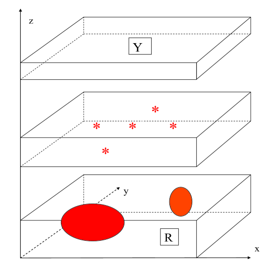
Figure 1: Geometric registration scheme of the inverse problem data: $R$ is a region of wave field scatterers, $Y$ is a domain of registration for the data $V_{2}(x)$, «stars» are conditional positions of field sources.

3 The scheme of data registration for the inverse problem and special form of the basic integral equation

The inverse problem of finding the function $c(x)$ is reduced to solving a linear integral equation (6) with known right-hand side, obtained from the measurement of the function $\frac{\partial V_{2}(x)}{\partial x_{3}}$ in $Y$ and calculations of the integrals standing in right side of (6). In this paper, we consider a specific scheme for the registration of the data, that is the function $\frac{\partial V_{2}(x)}{\partial x_{3}}$, ’’in a flat layer’’.

Below, for convenience we take for the variables $x_{1},x_{2},x_{3}$ the usual notation $x,y,z$. Figure 1 shows schematically the geometry of the problem, with the region $R$ of heterogeneities, which scatter the incident waves, and the domain $Y$, in which the scattered field is registered. The domain $Y$ has a form of endless flat layer in variables $x,y$, which is perpendicular to the axis $Oz$. The bounded region $R$ belongs to a similar layer. The asterisks shows conditionally possible positions of the field sources.

Thus, we assume that $R=\mathbb{R}_{xy}^{2}\times[h,H],\,\,Y=\mathbb{R}_{xy}^{2}\times[h_{Y},H_{Y}]$ and consider Equation (6) in the form

$$\mathop{\int\!\!\!\!\int\!\!\!\!\int}\nolimits_{R}K\left(x-x^{\prime},y-y^{\prime},z-z^{\prime}\right)\zeta(x^{\prime},y^{\prime},z^{\prime})dx^{\prime}dy^{\prime}dz^{\prime}=U(x,y,z),\,\,\,(x,y,z)\in Y,$$ (8)

with the kernel

$$K(x,y,z)=\frac{\partial}{\partial z}\left(\frac{1}{\left(x^{2}+y^{2}+z^{2}\right)^{1/2}}\right)=-\frac{z}{\left(x^{2}+y^{2}+z^{2}\right)^{3/2}}$$

and the right-hand side $v$ given in (6). We transform Equation (8) in the following way:

$$\int_{h}^{H}dz^{\prime}\mathop{\int\!\!\!\!\int}\nolimits_{\mathbb{R}_{xy}^{2}}K(x-x^{\prime},y-y^{\prime},z-z^{\prime})\zeta(x^{\prime},y^{\prime},z^{\prime})dx^{\prime}dy^{\prime}=U(x,y,z),\,\,\,(x,y)\in\mathbb{R}_{xy}^{2},\,z\in[h_{Y},H_{Y}].$$

Assumptions about the function $\zeta(x,y,z)$ and definition of the functions $K(x,y,z)$ and $U(x,y,z)$ ensure the inclusions: $\zeta\in L_{2}(R),\,\,v\in L_{2}(Y)$; $\zeta(x^{\prime},y^{\prime},z^{\prime})\in L_{2}(\mathbb{R}_{xy}^{2}),\,\,v(x,y,z)\in L_{2}(\mathbb{R}_{xy}^{2})$ for all admissible $z,z^{\prime}$, as well as the following relations: $||K(x-x^{\prime},y-y^{\prime},z-z^{\prime})||_{L_{2}(Y\times R)}<\infty$, $||K(x,y,z-z^{\prime})||_{L_{2}(\mathbb{R}_{xy}^{2})}<\infty$, $\forall z,z^{\prime},\,z\in[h_{Y},H_{Y}],\,z^{\prime}\in[h,H]$. Then, using the two-dimensional Fourier transforms $\tilde{K}(\omega_{1},\omega_{2},z),\,\,\tilde{\zeta}(\omega_{1},\omega_{2},z)$, $\tilde{v}(\omega_{1},\omega_{2},z)$ of these functions in the variables $(x,y)$ and taking into account the convolution theorem, we obtain a family of one-dimensional integral equations of the first kind

$$\int_{h}^{H}\tilde{K}(\omega_{1},\omega_{2},z-z^{\prime})\tilde{\zeta}(\omega_{1},\omega_{2},z^{\prime})dz^{\prime}=\tilde{v}(\omega_{1},\omega_{2},z),\,\,z\in[h_{Y},H_{Y}].$$ (9)

The equation (8) can be written in the operator form $A\zeta=v$ with linear and bounded integral operator $A:L_{2}(R)\rightarrow L_{2}(Y)$. Also, we represent Equations (9) in the operator form $A(\omega_{1},\omega_{2})\tilde{\zeta}=\tilde{v}(\omega_{1},\omega_{2},z)$ with bounded linear integral operators $A(\omega_{1},\omega_{2})[\cdot]=\int_{h}^{H}\tilde{K}(\omega_{1},\omega_{2},z-z^{\prime})[\cdot]dz^{\prime}$ acting from $L_{2}[h,H]$ to $L_{2}[h_{Y},H_{Y}]$.

It is well known that the solution to the integral equation of the form

$$\int_{R}\frac{\partial}{\partial x_{3}}\left(\frac{1}{\left|x-x^{\prime}\right|}\right)\zeta(x^{\prime})dx^{\prime}=v(x),\,\,x\in Y,$$ (10)

may be non-unique in the class of functions $\zeta(x)$, which we consider. In particular, this is true for the equation (8). This means that the null-space $N(A)$ of the operator $A$ contains non-trivial elements $\zeta=\zeta_{0}(x)$: $A\zeta_{0}=0$.

Assumption U. We assume that the required solution $\zeta=\bar{\zeta}(x)$ of the equation (8) satisfies the condition $(\bar{\zeta},\zeta_{0})_{L_{2}(R)}=0,\,\forall\zeta_{0}\in N(A)$.

This is consistent with our desire to be free as possible in the desired solution of the artefacts $\zeta_{0}(x)$, creating the observed zero function $v(x)$. Thus, we seek the unique normal solution $\zeta=\bar{\zeta}(x)$ of the linear operator equation $A\zeta=v$, that is Equation (8), in the space $L_{2}(R)$ assuming that this solution is continuous and finite, $\mathrm{supp}\,\bar{\zeta}\subset R$. Also, we do not exclude the case when $\bar{\zeta}(x)$ belongs to one of the uniqueness classes of solutions to the equation (10), which have been studied previously, for example, in the works [12, 13] and etc.

Currently, many stable methods, so called RAs, are known for finding normal solutions $\zeta=\bar{\zeta}\in Z$ of linear operator equations $A\zeta=v,\,v\in U,$ in Hilbert spaces $Z,U$ (see, e.g. [14, 15, 16, 19, 17] and etc). Suppose that a parametric family of operators $R_{\alpha}(A):U\rightarrow Z$ presents one of such methods. Assume that instead of $v$, we have at our disposal its approximation, that is an element $v_{\delta}\in U$, which meets the approximation condition $||v-v_{\delta}||_{U}\leq\delta$. Then, with a suitable choice of the parameter $\alpha=\alpha(\delta)$ the convergence of approximate solutions $\zeta_{\delta}=R_{\alpha(\delta)}(A)v_{\delta}$ takes place: $||\zeta_{\delta}-\bar{\zeta}||_{Z}\rightarrow 0$ as $\delta\rightarrow 0$. In particular, the regularity conditions for elements $\zeta_{\delta}$, that is

$$\overline{\lim_{\delta\rightarrow 0}}||\zeta_{\delta}||_{Z}\leq||\bar{\zeta}||_{Z},\,\,\lim_{\delta\rightarrow 0}||A\zeta_{\delta}-v_{\delta}||_{U}=0,$$ (11)

are sufficient for such convergence (see, e.g. [16, 20]).

4 Algorithm for solving the basic equation (8) and the stability of the algorithm

Algorithm 1.

1)Calculation of 2D Fourier transforms $\tilde{K}(\omega_{1},\omega_{2},z)$ и $\tilde{v}(\omega_{1},\omega_{2},z)$ for each $z\in[h,H]$.

2) For each $(\omega_{1},\omega_{2})$, finding an approximate normal solution $\tilde{\zeta}_{\delta}(\omega_{1},\omega_{2},z)$ of the integral equation (9) via an RA, which ensures the regularity conditions of the form

$$||\tilde{\zeta}_{\delta}(\omega_{1},\omega_{2},z)||_{L_{2}(R_{\omega_{1}\omega_{2}}^{2})}\leq||\bar{\zeta}(\omega_{1},\omega_{2},z)||_{L_{2}(\mathbb{R}_{\omega_{1}\omega_{2}}^{2})},$$ (12)

$$\lim_{\delta\rightarrow 0}\left\|A(\omega_{1},\omega_{2})\widetilde{\zeta}_{\delta}(\omega_{1},\omega_{2},z)-\widetilde{v}_{\delta}(\omega_{1},\omega_{2},z)\right\|_{L_{2}(\mathbb{R}_{\omega_{1}\omega_{2}}^{2})}=0,~{}\ \forall z\in[h,H].$$ (13)

3) For each $z\in[h,H]$, calculating an approximate solution of the equation (8) using 2D inverse Fourier transform $F^{-1}$ in the variables $(x,y)$:

$$\zeta_{\delta}(x,y,z)=F^{-1}[\tilde{\zeta}_{\delta}(\omega_{1},\omega_{2},z)](x,y).$$

4) Finding the function $\xi_{\delta}(x,y,z)=\zeta_{\delta}(x,y,z)/V_{0}(x,y,z)$, which approximates the value $\xi(x,y,z)=\frac{1}{c_{0}^{2}}-\frac{1}{c^{2}(x,y,z)}$ and calculating the approximation for $c(x,y,z)$ from the last equality.

Note that the conditions (12) and (13) hold true for Tikhonov regularization, if we select the parameter $\alpha(\delta)$ using the discrepancy principle [16] or its generalization [20]. The same property has the TSVD method (see, e.g. [18, 19]) under suitable choice of the regularization parameter.

Now, we turn to the justification of the stability of the proposed Algorithm 1.

Lemma 1

Let $\{\tilde{\zeta}_{\omega_{1}\omega_{2}}^{(norm)}(z)\}\in L_{2}[h,H]$ be a family of normal solutions to the equations (9) for all considered values $\omega_{1},\omega_{2}$. Then the equality holds: $\bar{\zeta}(x,y,z)=F^{-1}\left[\tilde{\zeta}_{\omega_{1}\omega_{2}}^{(norm)}(z)\right](x,y)$.

Proof. We introduce the element $\zeta^{(norm)}(x,y,z)=F^{-1}\left[\tilde{\zeta}_{\omega_{1}\omega_{2}}^{(norm)}(z)\right](x,y)$ and denote 2D Fourier transform of the normal solution $\bar{\zeta}(x,y,z)$ to the equation (8) as $\tilde{\bar{\zeta}}(\omega_{1},\omega_{2},z)$. The following Plancherel equalities are valid for all $z\in[h,H]$:

$$\iint\limits_{\mathbb{R}_{xy}^{2}}\left[\zeta^{(norm)}(x,y,z)\right]^{2}dxdy=\frac{1}{4\pi^{2}}\iint\limits_{\mathbb{R}_{\omega_{1}\omega_{2}}^{2}}\left[\tilde{\zeta}_{\omega_{1}\omega_{2}}^{(norm)}(z)\right]^{2}d\omega_{1}d\omega_{2},\\ \iint\limits_{\mathbb{R}_{xy}^{2}}\left[\bar{\zeta}(x,y,z)\right]^{2}dxdy=\frac{1}{4\pi^{2}}\iint\limits_{\mathbb{R}_{\omega_{1}\omega_{2}}^{2}}\left[\tilde{\bar{\zeta}}(\omega_{1},\omega_{2},z)\right]^{2}d\omega_{1}d\omega_{2}.$$

The function $\tilde{\bar{\zeta}}(\omega_{1},\omega_{2},z)$ satisfies the equations (9) for all $z\in[h,H]$. Therefore

$$\left\|\zeta_{\omega_{1}\omega_{2}}^{(norm)}(z)\right\|_{L_{2}[h,H]}^{2}=\int\limits_{h}^{H}\left[\tilde{\zeta}_{\omega_{1}\omega_{2}}^{(norm)}(z)\right]^{2}dz\leq\int\limits_{h}^{H}\tilde{\bar{\zeta}}^{2}(\omega_{1},\omega_{2},z)dz=\left\|\tilde{\bar{\zeta}}(\omega_{1},\omega_{2},z)\right\|_{L_{2}[h,H]}^{2}.$$

Combining these relations and applying Fubini’s theorem, we obtain

$$\left\|\zeta^{(norm)}(x,y,z)\right\|_{L_{2}(R)}^{2}=\int\limits_{h}^{H}dz\iint\limits_{\mathbb{R}_{xy}^{2}}\left[\zeta^{(norm)}(x,y,z)\right]^{2}dxdy=\\ =\frac{1}{4\pi^{2}}\int\limits_{h}^{H}dz\iint\limits_{\mathbb{R}_{\omega_{1}\omega_{2}}^{2}}\left[\tilde{\zeta}_{\omega_{1}\omega_{2}}^{(norm)}(z)\right]^{2}d\omega_{1}d\omega_{2}=\frac{1}{4\pi^{2}}\iint\limits_{\mathbb{R}_{\omega_{1}\omega_{2}}^{2}}\left\|\zeta_{\omega_{1}\omega_{2}}^{(norm)}(z)\right\|_{L_{2}[h,H]}^{2}d\omega_{1}d\omega_{2}\leq\\ \leq\frac{1}{4\pi^{2}}\iint\limits_{\mathbb{R}_{\omega_{1}\omega_{2}}^{2}}\left\|\tilde{\bar{\zeta}}(\omega_{1},\omega_{2},z)\right\|_{L_{2}[h,H]}^{2}d\omega_{1}d\omega_{2}=\frac{1}{4\pi^{2}}\int\limits_{h}^{H}dz\iint\limits_{\mathbb{R}_{\omega_{1}\omega_{2}}^{2}}\left[\tilde{\bar{\zeta}}(\omega_{1},\omega_{2},z)\right]^{2}d\omega_{1}d\omega_{2}=\\ =\int\limits_{h}^{H}dz\iint\limits_{\mathbb{R}_{xy}^{2}}\left[\bar{\zeta}(x,y,z)\right]^{2}dxdy=\left\|\bar{\zeta}(x,y,z)\right\|_{L_{2}(R)}^{2}.$$

By the uniqueness of the normal solution to the equation (8), this implies equality $\bar{\zeta}(x,y,z)=\zeta^{(norm)}(x,y,z)=F^{-1}\left[\tilde{\zeta}_{\omega_{1}\omega_{2}}^{(norm)}(z)\right](x,y)$. $\square$

Theorem 1

Algorithm 1 ensures the convergence $\left\|\zeta_{\delta}(x,y,z)-\bar{\zeta}(x,y,z)\right\|_{L_{2}(R)}\rightarrow 0$ as $\delta\rightarrow 0$.

Proof. We define for $z\in[h,H]$ the family of the functions

$$\eta_{\delta}(z)=\left\|\tilde{\zeta}_{\delta}(\omega_{1},\omega_{2},z)-\tilde{\zeta}_{\omega_{1}\omega_{2}}^{(norm)}(z)\right\|_{L_{2}\left(\mathbb{R}_{\omega_{1}\omega_{2}}^{2}\right)}^{2}=\left\|\tilde{\zeta}_{\delta}(\omega_{1},\omega_{2},z)-\tilde{\bar{\zeta}}(\omega_{1},\omega_{2},z)\right\|_{L_{2}\left(\mathbb{R}_{\omega_{1}\omega_{2}}^{2}\right)}^{2}.$$

The dual form of this family’s representation follows from Lemma 1. The properties (12) and (13) of the used RA guarantee for every $z\in[h,H]$ the convergence of approximate solutions $\tilde{\zeta}_{\delta}(\omega_{1},\omega_{2},z)$ to normal solutions $\tilde{\zeta}_{\omega_{1}\omega_{2}}^{(norm)}(z)$ in the space $L_{2}\left(\mathbb{R}_{\omega_{1}\omega_{2}}^{2}\right)$ as $\delta\rightarrow 0$. Therefore, $\lim_{\delta\rightarrow 0}\eta_{\delta}(z)=0,~{}\forall z\in[h,H]$. Besides, the conditions (12) and the inequality

$$0\leq\eta_{\delta}(z)\leq\left(\left\|\tilde{\zeta}_{\delta}(\omega_{1},\omega_{2},z)\right\|_{L_{2}\left(\mathbb{R}_{\omega_{1}\omega_{2}}^{2}\right)}+\left\|\tilde{\bar{\zeta}}(\omega_{1},\omega_{2},z)\right\|_{L_{2}\left(\mathbb{R}_{\omega_{1}\omega_{2}}^{2}\right)}\right)^{2}\leq\\ \leq 4\left\|\tilde{\bar{\zeta}}(\omega_{1},\omega_{2},z)\right\|_{L_{2}\left(\mathbb{R}_{\omega_{1}\omega_{2}}^{2}\right)}^{2}\equiv s(z)$$

imply that the functions $\eta_{\delta}(z)$ have integrable majorant $s(z)$. Then the convergence to be proved can be derived from the corresponding Plancherel equality and Lebesgue’s theorem on passage to the limit in the following way:

$$\lim_{\delta\rightarrow 0}\left\|\zeta_{\delta}(x,y,z)-\bar{\zeta}(x,y,z)\right\|_{L_{2}(R)}^{2} = \lim_{\delta\rightarrow 0}\frac{1}{4\pi^{2}}\int\limits_{h}^{H}\left\|\tilde{\zeta}_{\delta}(\omega_{1},\omega_{2},z)-\tilde{\bar{\zeta}}(\omega_{1},\omega_{2},z)\right\|_{L_{2}\left(\mathbb{R}_{\omega_{1}\omega_{2}}^{2}\right)}^{2}dz=$$

$$= \lim_{\delta\rightarrow 0}\frac{1}{4\pi^{2}}\int\limits_{h}^{H}\eta_{\delta}(z)dz=0.\,\,\square$$

5 Finite-dimensional approximation of the problem and the numerical implementation of the algorithm

We replace in (6) and (8) the space $\mathbb{R}^{3}$ by the region $\Pi=[-r,r]\times[-r,r]\times[-r,r]$ and the space $\mathbb{R}^{2}_{xy}$ by the rectangle $\Pi_{xy}=[-r,r]\times[-r,r]$ with $r>0$ ’’large enough’’. We carry out an approximation of equations (8) and (9) in the domain $\Pi$ by the finite difference method introducing uniform grids for $x,\omega_{1}\in[-r,r]$ and $y,\omega_{2}\in[-r,r]$ of the size $N$, as well as the grids for $z,z^{\prime}$: $\left\{z_{i}\right\}\in[h_{Y},H_{Y}],\,\,\left\{z^{\prime}_{j}\right\}\in[h,H]$ of the size $M$ and $M^{\prime}$ respectively. After that, we apply 2D fast Fourier transform in the first section of Algorithm 1 for calculation of discrete analogues of the functions $\tilde{K}(\omega_{1},\omega_{2},z)$, $\tilde{v}(\omega_{1},\omega_{2},z)$. In the second section of Algorithm 1 we approximate integrals in (9) using quadrature and obtain $N^{2}$ systems of linear algebraic equations for subsequent solution:

$$A^{(m)}\tilde{\zeta}^{(m)}=\tilde{U}^{(m)},\,\,m=1,...,N^{2}.$$ (14)

Here $A^{(m)}=\left[\nu_{ij}\tilde{K}(\omega_{1}^{(m)},\omega_{2}^{(m)},z_{i}-z^{\prime}_{j})\right]$ are matrices of the size $M\times M^{\prime}$ and $\tilde{U}^{(m)}=[\tilde{U}(\omega_{1}^{(m)},\omega_{2}^{(m)},z_{i})]$ are columns of the length $M$. The values $\left(\omega_{1}^{(m)},\omega_{2}^{(m)}\right)$ are grid points for the variables $(\omega_{1},\omega_{2})$ numbered by a single superscript $m$ and $\nu_{ij}$ are quadrature coefficients. The SLAEs (14) was solved by application of the RAs with properties (12) and (13).

In doing so, we used a number of RAs, namely, Tikhonov regularization in the standard and iterated form, the TSVD method and some others (for their implementation, see e.g. [2, 3, 17, 21, 18, 19, 20]). Numerical experiments have shown that the best results in the regularization of systems (14) gives the TSVD method. The results of its application are presented in the following section.

6 Model example

We write the equation (6) formally, regardless of Assumptions 1) - 5), for the function $\varphi(x)\,=\sum_{l=1}^{L}\delta(x-x_{l}),\,\,x_{l}\notin R,\,\,x_{l}\notin Y$. Then

$$V_{0}(x)=-\frac{A_{0}}{4\pi}\sum_{l=1}^{L}{\frac{1}{\left|x-x_{l}\right|}},$$

and the equation (6) takes the form

$$\int_{R}\frac{\partial}{\partial x_{3}}\left(\frac{1}{\left|x-x^{\prime}\right|}\right)\zeta(x^{\prime})dx^{\prime}=\\ =2\pi\frac{\partial V_{2}(x)}{\partial x_{3}}+\frac{A_{2}}{2}\sum_{l=1}^{L}\frac{\partial}{\partial x_{3}}\left(\frac{1}{\left|x-x_{l}\right|}\right)-\frac{A_{0}}{4\pi c_{0}^{2}}\sum_{l=1}^{L}\int_{\mathbb{R}^{3}}\frac{\partial}{\partial x_{3}}\left(\frac{1}{\left|x-x^{\prime}\right|}\right)\frac{dx^{\prime}}{\left|x^{\prime}-x_{l}\right|},\,\,\,x\in Y.$$ (15)

This form of the integral equation can be used for the finite-dimensional approximation as in Section 5, with ’’sufficiently fine’’ grids, meaning $\delta(x-x_{l})$ to be some smooth $\delta$-shaped family of finite functions on these grids

Keeping in mind the experimental scheme shown in Figure 1, we define a model solution

$$\begin{array}[]{l}{\xi(x,y,z)=a_{1}\exp\left(-x^{2}-2y^{2}\right){\rm+}a_{2}\exp\left[-3(x+4)^{2}-(y-5)^{2}+(x+4)(y-5)\right]+}\\ {+a_{3}\exp\left\{-0.9\left[(x-4)^{2}-(y+4)^{2}+(x-4)(y+4)\right]\right\}}\end{array}$$

with

$$\begin{array}[]{l}{a_{1}=\left(1-4(z-1.5)^{2}\right)^{2},\,\,a_{2}=0.4\max\left\{1-(z_{0}-1.3)^{2}{\rm,\;}0\right\}},\\ {a_{3}=0.2\max\left\{\left[1-(z_{0}-1.7)^{2}\right]^{{\rm 2}}{\rm,\;}0\right\}}\end{array}$$

and $(x,y,z)\in R=[-10,10]\times[-10,10]\times[1,2]$. Registration domain of the scattered wave field is represented as $Y=[-10,10]\times[-10,10]\times[6,7]$. We use ten $\delta$-shaped sources whose positions are given by the points

$$\,(x_{l},y_{l},z_{l})=(0,0,z_{0}),\,(-r,0,z_{0}),(r,0,z_{0}),(0,-r,z_{0}),(0,r,z_{0});\,\,\,z_{0}=3,5;\,\,\,r=8.$$

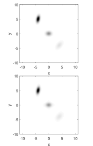
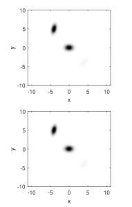
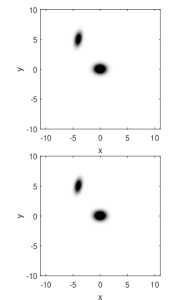
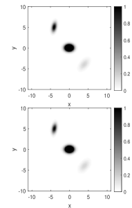
Figure 2: A qualitative comparison of the exact (top) and an approximate (bottom) solutions to the inverse problem for the unperturbed data: from left to right $z$= 1.035, 1.094, 1.191, 1.582.

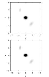
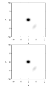
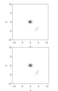
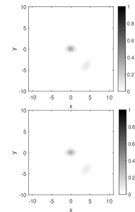
Figure 3: A qualitative comparison of the exact (top) and an approximate (bottom) solutions to the inverse problem for the unperturbed data: from left to right $z$= 1.777, 1.875, 1.934, 1.973.

We also assume that $g(t)=\exp(-t)$ and $c_{0}=0.5$. Then we compute the discrete analogue of the experimental data

$$\frac{\partial V_{2}(x)}{\partial x_{3}}=\frac{1}{2\pi}\{\int_{R}\frac{\partial}{\partial x_{3}}\left(\frac{1}{\left|x-x^{\prime}\right|}\right)\zeta(x^{\prime})dx^{\prime}-\frac{A_{2}}{2}\sum_{l=1}^{L}\frac{\partial}{\partial x_{3}}\left(\frac{1}{\left|x-x_{l}\right|}\right)+\\ +\frac{A_{0}}{4\pi c_{0}^{2}}\sum_{l=1}^{L}\int_{\Pi}\frac{\partial}{\partial x_{3}}\left(\frac{1}{\left|x-x^{\prime}\right|}\right)\frac{dx^{\prime}}{\left|x^{\prime}-x_{l}\right|}\},\,\,\,x\in Y,$$

in (15), using a discrete Fourier transform (algorithmically, fast Fourier transform) as described above. In so doing, we obtain the data of the inverse problem, $\frac{\partial V_{2}(x)}{\partial x_{3}}$, with errors associated with finite-dimensional approximation in calculation of the integrals. After that we form the right-hand sides of the discrete equations (14) and solve them by the TSVD method. Finally, we calculate the function $\xi(x,y,z)=\frac{\zeta(x,y,z)}{V_{0}(x,y,z)}$. We confine ourselves to the calculation of this particular function, not $c(x)$, because examine the procedure for solving linear equations (15).

Figures 2 and 3 show, for several values of $z\in[1,2]$, the exact solution $\xi_{exact}(x,y,z)$ (top) and calculated approximate solution $\xi_{appr}(x,y,z)$ (below) in pairs for qualitative comparisons. The quantitative dependence of obtained relative accuracy,

$$\Delta_{C}(z)=\frac{\left\|\xi_{appr}(x,y,z)-\xi_{exact}(x,y,z)\right\|_{C(\mathbb{R}_{xy}^{2})}}{\left\|\xi_{exact}(x,y,z)\right\|_{C(\mathbb{R}_{xy}^{2})}},$$

for the approximate solution $\xi_{appr}(x,y,z)$ in the layer $z=\mathrm{const}$ is shown in Fig. 4 by solid line. The calculations were performed in MATLAB on PC with a processor Intel (R) Core (TM) i7-2600 CPU 3.40 GHz, RAM 8GB without parallelization.

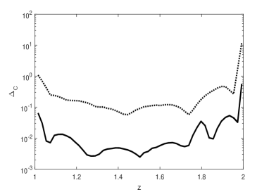
Figure 4: The relative accuracy $\Delta_{C}(z)$ of approximate solution (in the norm of $C(\mathbb{R}_{xy}^{2})$) for different $z$. Solid line: the value $\Delta_{C}(z)$ for for the unperturbed data, dotted line: $\Delta_{C}(z)$ for perturbed data with a maximum perturbation value about 1e-8.

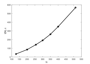
Figure 5: The solving time vs $N$.

Since we are talking about the creation of a fast solution algorithm for our inverse problem, we point out some of its temporal characteristics. The dimensions of grids in the variables $z,z^{\prime}$, i.e, the values of $M,\,M^{\prime}$, determine the speed of solving the one-dimensional integral equation (9) at fixed $\omega_{1},\omega_{2}$, that is the SLAE (14) for a fixed $m$. The corresponding solution time, $t_{0}(M,M^{\prime})$, varies a little in passing from one of equations (9) to another. This time is controlled by the desired resolution of the algorithm in the variable $z$. Actually, we have the estimate $t(N,M,M^{\prime})\approx t_{0}(M,M^{\prime})\cdot N^{2}$ for full-time inverse problem solution on chosen grids, and the number $N$ is controlled here by required resolution in $x,y$. We present in Figure 5 the dependence $t(N)=t(N,M,M^{\prime})$ calculated on the same computer for fixed $M=51,M^{\prime}=51$ and for different $N$. In particular, the time to solve the 3D inverse problem for $N=512$ is less than 10 minutes.

Note that the inverse problem under consideration is extremely sensitive to errors in the input data. In solving it with the double precision, small perturbations in the right side of the SLAEs (14) by random errors with the level of the order of 1e-8 lead to excessive smoothing of the approximate solution when used the TSVD method and Tikhonov regularization.

The reason is very fast decay of singular values of the matrices $A^{(m)}$ in the system (14). The graph characterizing their behavior for a typical matrix $A^{(m)}$ is shown in Figure 6. When using the TSVD method for the solution of SLAEs (14), the small singular values are rejected [18, 19]. In our case, for the inverse problem data computed with the approximation error, but without the additional perturbation by random error, singular values of the order 1e-12 – 1e-13 or less are discarded. The remainder of a singular basis, 15 - 25 elements are used in the solution of (14) and allow to reproduce the desired solution of the inverse problem relatively accurate (see Figure 4, solid line). The introduction of random errors of the order of 1e-10 – 1e-8 in the data drastically reduces the dimension of used singular basis (to 4 – 5 elements), and this leads to a ’’oversmoothed’’ approximate solution, i.e. to its poor accuracy (see Figure 4, dotted line). Approximately the same effect occurs when using Tikhonov regularization. However, the degree of oversmoothness for approximate solution is more than for the TSVD. The corresponding theoretical error estimates under different a priori assumptions can be found in [2, 3].

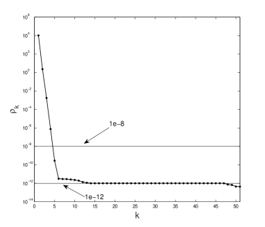
Figure 6: Dependence of singular values $\rho_{k}$ of a matrix $A^{(m)}$ on their number $k$.

Summing up the results of this work, we can draw the following conclusions.

1. The inverse coefficient problem for the wave equation, arising in modeling acoustic sensing, can be solved numerically faster if instead of the time dependence $u(x,t)$ of the scattered field in a region $Y$ we take as input data some integrals of $u(x,t)$ in time. One possible integral of such a kind is the function $V_{2}(x)$ or its partial derivatives.

2. For this type of data recorded in the plane layer, it is possible to propose a numerical algorithm, which allows to solve the inverse problem on a personal computer without the use of supercomputer systems, in a relatively short period of time, for sufficiently fine grids.

The work was supported by the Russian Foundation for Basic Research (grants nos. 16-01-00039 and 15-01-00026а).

References

[1] L. Beilina and M.V. Klibanov, Approximate
Global Convergence and Adaptivity for Coefficient Inverse Problems.
New York: Springer, 2012.
[2] A.B. Bakushinsky, M.Yu. Kokurin,
Iterative methods for approximate solution of inverse problems.
Mathematics and Its Applications. Dordrecht: Springer, 2004.
[3] A.B. Bakushinsky, M.Yu. Kokurin,
Iterative methods of solving ill-posed operator equations with smooth
operators. Moscow: Editorial URSS, 2002 (in Russian).
[4] A.V. Goncharskii, S.Yu. Romanov, Two
approaches to the solution of coefficient inverse problems
for wave equations. Computational Mathematics and Mathematical
Physics, 2012, 52:2, 245–251.
[5] A.V. Goncharskii, S.Yu. Romanov, Supercomputer
technologies in the development of methods for solving
inverse problems in ultrasound tomography. Numerical
Methods and Programming. Scientific on-line open access
journal. 2012, 13:1, 235-238 (in Russian).
[6] A.B. Bakushinskii, A.I. Kozlov, M.Yu.
Kokurin, On some inverse problem for a three-dimensional wave
equation. Computational Mathematics and Mathematical Physics,
2003, 43:8, 1149–1158.
[7] A.N. Tikhonov and A.A. Samarskii, Equations
of Mathematical Physics. New York, Dover Publications, inc.
1963.
[8] S.L. Sobolev, Applications of Functional
Analysis in Mathematical Physics. American Mathematical
Society, Providence, Rhode Island, 1963.
[9] L. Go̊rding, Cauchy’s Problem for
Hyperbolic Equations, University of Chicago, 1957.
[10] B.R. Vainberg, On a point source in an
inhomogeneous medium. Mathematics of the USSR-Sbornik
(1974),23(1):123.
[11] V.S. Vladimirov, Methods of the Theory of
Generalized Functions, Taylor and Francis, London and New York,
2002.
[12] V.N. Strakhov, On the equivalence in an
inverse gravimetric problem with variable mass density,
Doklady AN SSSR, 1977, v. 236, N 2, p. 329-331 (in Russian).
[13] A.I. Prilepko, Exterior contact inverse
problems of generalized magnetic potentials of variable
densities, Differensial’nye Uravneniya 6 (1970), 39-49 (in Russian).
[14] A. Bakushinsky and A. Goncharsky, Ill-Posed
Problems: Theory and Applications, Kluwer Academic
Publishers, Dordrecht, 1994.
[15] G.M. Vainikko and A.Y. Veretennikov, Iterational
Procedures in Ill-Posed Problems, Wiley, New York, 1985.
[16] V.A. Morozov, Methods for Solving
Incorrectly
Posed Problems, Springer-Verlag, New York, 1984.
[17] A.N. Tikhonov, A.V. Goncharsky, V.V. Stepanov
and A.G. Yagola, Numerical Methods for the Solution of
Ill-Posed Problems, Dordrecht, Kluwer, 1995.
[18] R.J. Hanson, A numerical method for solving
Fredholm integral equations of the first kind using
singular values, SIAM J. Numer. Anal., 8 (1971), pp.
616-622.
[19] H.W. Engl, M. Hanke and A. Neubauer
Regularization of Inverse Problems. Dordrecht:
Kluwer, 1996.
[20] A. N. Tikhonov, A. S. Leonov and A. G. Yagola,
Non-Linear Ill-Posed Problems (in Russian), Nauka, Moscow,
1995; translation published by Chapmen Hall, London,
1998.
[21] A.S. Leonov, Solution of Ill-Posed Inverse
Problems. Theory Review, Practical Algorithms and MATLAB
Demonstrations, Librokom, Moscow, 2010 (in Russian).