Runtime Optimization of Join Location in Parallel Data Management Systems

Abstract

Applications running on parallel systems often need to join a streaming relation or a stored relation with data indexed in a parallel data storage system. Some applications also compute UDFs on the joined tuples. The join can be done at the data storage nodes, corresponding to reduce side joins, or by fetching data from the storage system to compute nodes, corresponding to map side join. Both may be suboptimal: reduce side joins may cause skew, while map side joins may lead to a lot of data being transferred and replicated.

In this paper, we present techniques to make runtime decisions between the two options on a per key basis, in order to improve the throughput of the join, accounting for UDF computation if any. Our techniques are based on an extended ski-rental algorithm and provide worst-case performance guarantees with respect to the optimal point in the space considered by us. Our techniques use load balancing taking into account the CPU, network and I/O costs as well as the load on compute and storage nodes. We have implemented our techniques on Hadoop, Spark and the Muppet stream processing engine. Our experiments show that our optimization techniques provide a significant improvement in throughput over existing techniques.

1 Introduction

Parallel batch data processing systems such as Hadoop MapReduce and Spark [29] are designed to process massive amounts of data on a large cluster of machines. Parallel stream processing systems, such as Storm [28] and Muppet [15], on the other hand, are aimed at processing a fire-hose of data that arrive at very fast rates. These frameworks work on many nodes and are designed to serve different ends of the spectrum in terms of latency and throughput. Systems such as HBase and Cassandra are often used as backend data stores and support indexed access on primary keys.

In this paper, we consider a class of applications that run on such parallel systems and need to perform a join of input data, which may be streaming or stored data, with other data stored and indexed in a parallel data store. The application may also compute a UDF based on the joined tuples. There are numerous such applications that compute UDFs on join results, such as entity annotation using large stored models on streaming/stored textual data and genome sequence read alignment. We discuss a few applications later in Section 2. The focus of this work is on joins where the data stored in the parallel data store is indexed on the join attributes. (In case the data is not already indexed, an index can be created before computing the join.)

We refer to the nodes on which the application is running as compute nodes, and the nodes on which the data is stored as data nodes. A schematic representation of our architecture is shown in Figure 1.

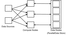
Figure 1: Parallel data management system with datastore access (data sources can have stored or streaming data)

Joins may be performed in different ways.

1. One way to perform the join is to fetch data from the data store, for each incoming stream/stored relation tuple, and execute the join (and UDF computation, if any) at the compute node. This is analogous to a map-side join or a parallel index nested-loops join.

   With a naive implementation for accessing data from the parallel data store, for each request sent to the data store, the compute node must wait for the result to come back, and then complete the computation, before moving on to the next data item. Such an implementation could be very inefficient due to high latencies for fetching data from the data store. Batching and asynchronous submission can be used to improve performance. However, this approach requires more data transfer if the UDF result is smaller than the input.

2. An alternative technique is to send the incoming tuples from the compute nodes to the data nodes and perform the join (along with the UDF computation, if any) at the data node. This technique is analogous to reduce-side join. Note that parallel hash joins used in parallel relational databases also correspond to reduce-side join. The build relation can be partitioned and indexed at the data nodes while nodes with the probe relation can be used as compute nodes.

   A drawback of the reduce side join approach is that it is vulnerable to skew if the input tuples have keys that are very frequent (heavy hitters) or the cost of UDF computation is higher for some key values. Such skew could result in some data nodes performing significantly more computations compared to other data nodes. Existing techniques to handle skew in parallel joins are based on using statistics or sampling to find balanced partitioning boundaries; in addition, some techniques such as [10, 23] also use statistics to find and replicate heavy hitters (very frequent keys). As described later in Section 2.1, these techniques can be extended to mitigate skew in entity annotation application. However, the techniques proposed earlier require a fixed threshold parameter to determine which keys are heavy hitters. In a streaming setting, statistics may be unavailable prior to execution and may change over time. Another technique to mitigate skew is to dynamically reallocate partitions to less loaded machines. However, this may be ineffective against skew caused by a single key or few keys.

A key idea in this paper is to process incoming tuples by dynamically deciding whether to perform the join by fetching values from the parallel data store (corresponding to map-side join), or by sending values to the parallel data store (corresponding to reduce-side join). One of these alternatives is chosen at runtime on a per join-key basis, depending on the frequency of the key and on the load at the compute and data nodes. Our goal is to optimize data access and computation, and minimize skew in this setting, in order to improve throughput.

Our main contributions in this paper are as follows.

1. We address the issue of dynamically deciding whether to perform the join at the compute or the data node using a ski-rental formulation. We give an overview of our framework in Section 3. We then present, in Section 4, generalizations of the classical ski-rental [13] problem along with worst-case performance guarantees. The generalized ski-rental is used to decide which items from the data store are being accessed frequently enough to be fetched from the data store and cached locally.

2. In Section 5, we present techniques that allow the computation to be balanced between compute nodes and data nodes with the goal of maximizing the throughput.

3. Our techniques are able to mitigate skew without any pre-computed statistics and work well with batch systems as well as with streaming systems, where statistics may not be available, and heavy hitters may change over time. Using our technique, heavy hitter keys would end up being cached across all compute nodes and would be processed at the compute nodes. Requests for infrequent keys, on the other hand, are sent to the data node and can be processed at the data node. Our techniques thus represent an alternative to existing techniques to handle hash join skew based on statistics, such as [10, 23].

   Our techniques allow dynamic addition and deletion of compute nodes since the compute nodes do not store intermediate join results or any state (other than cached data). In the context of streaming data, such elasticity can be used to add resources to handle peak load, while using less resources at low load.

4. Our runtime techniques can be used in the context of multiple joins (as described in Section 6), where statistics of intermediate join results may not be available.

5. We have also extended the APIs of the MapReduce, Spark and Muppet frameworks to incorporate the techniques of batching and prefetching. We describe these extensions in Section 7. Our techniques can also be used in traditional parallel relational databases.

6. We conduct several experiments, as described in Section 9, based on an entity annotation application as well as using some synthetic applications. We show that our optimization techniques provide significantly better throughput compared to alternatives for both batch processing and stream processing. In fact, our techniques perform better than a custom partitioner described in [12] to mitigate skew for the entity annotation implementation.

We provide a detailed comparison with related work in Section 8.

2 Motivating Applications

In this section, we use the example of entity annotation to motivate the need for our framework and also as a running example throughout this paper to demonstrate our optimization techniques. We also discuss other motivating applications.

2.1 Entity Annotation

Entity annotation is the problem of marking up words in a document with the entities that they refer to. Entity annotation can be done using trained machine learning models. For each “token”, i.e. name/word, a model is precomputed and stored, indexed by the token. To annotate a document, in the first step, tokens which are possible mentions of entities are identified, e.g. ‘Michael Jordan’, along with the surrounding text. In the next step, a classification function is applied on the model corresponding to the token along with text surrounding the token, to identify the entity which the token refers to: ‘Michael Jordan’, the basketball player or ‘Michael Jordan’, the computer scientist and professor.

A reduce-side join can be used for entity annotation. Models are partitioned amongst reducers. A mapper extracts tokens, with surrounding text, and maps it based on tokens. The reducer joins the token with the models and performs classification using models.

map(docId,document) {
 for each spot in document.getSpots(){
  spotContext = getContextRecord(spot,document)
  context.write(spotContext.key, spotContext.value)
 }
}
partitioner(key) {
 if(isFrequent(key)) {
  //spread across multiple reducers
  return randomPartition
 } else {
  //to localise access to stored models
  return getPartition(key)
 }
}
reduce(key,values) {
 model = getModel(key)
 for each spotContext in values {
  annotatedValues =
    classifyRecord(spotContext, model)
  context.write(annotedValues)
 }
}

Figure 2: Entity annotations with join at reduce

map(docId,document) {
 for each spot in document.getSpots(){
  spotContext=getContextRecord(spot,document)
  annotatedValues =
      f(spotContext.key,spotContext.value)
  context.write(spotContext.key, annotatedValues)
 }
}
f(key,params) {
 model = modelStore.getModel(key)
 annotatedValues = classifyRecord(params,model)
 return annotatedValues
}

Figure 3: Entity annotations with map-side joins

Gupta et al. show in [12] that entity annotation using reduce-side join is inefficient because of skew, and present a custom partitioning function to mitigate skew due to both key frequency and classification function computation cost imbalance across different models. To reduce skew, models with high costs due to frequent tokens or high classification cost are replicated across all partitions; models with low costs are kept at one partition. Pseudo code for their approach is shown in Figure 2. In the map function, spotContext.key is the token and spotContext.value is the surrounding text. Frequent tokens are routed randomly to any one of the reducers while non frequent ones are routed to the same partition as the model for the token. Their solution may be viewed as an extension of the work by DeWitt et al. [10], for minimizing parallel join skew, since they use a similar partitioning/replication technique, but [12] also take the computation time for the classification function into account.

Entity annotation can also be done at the map side by fetching models to the mapper and performing the annotations at the mapper. Sample pseudocode for this approach is shown in Figure 3, where $f(key,params)$ is the function that performs the entity annotation. However, if done naively, this approach will lead to a lot of data being transferred from the data store and data accesses would be blocking, making it inefficient.

Our approach performs the join as part of the map function but, for each token, chooses between fetching the model and performing annotation at the mapper, versus sending the token with surrounding text to the nodes hosting the models.

Our approach can also be used to annotate entities in a text stream. For example, entity annotation is important for Twitter streams [7]. For a Twitter stream, new events which did not exist earlier may suddenly gain popularity. Hence, it may not be possible to use pre-computed statistics to decide frequent keys. On the other hand, our approach does not assume any distribution, but computes statistics at runtime, allowing it to adapt to changes.

2.2 Other Applications

In general, our framework can be applied to applications that perform joins in a batch setting. It can also be used for stream-relation joins in a parallel setting.

Many machine learning models can make use of the parameter server framework described in [26] for efficient distributed implementation. In this framework, machine learning models can be represented as a set of $<$key,value$>$ pairs and can be shared across multiple nodes for parallel execution. Li et al. [16] show how batched access (which they define as range push and pull) and asynchronous tasks can lead to more efficient learning algorithms. Our techniques perform ski-rental based caching and dynamic load balancing in addition to batching and asynchronous calls.

CloudBurst [24] aligns a set of genome sequence reads with a reference sequence using MapReduce, executing a UDF as part of the reduce operation. Our framework could be used in this case to mitigate skew and reduce the runtime; details can be found in Appendix A. Our techniques can also be used to minimize skew for joins parallel database settings.

3 Framework and Solution
Approach

In this section, we give an overview of our general framework. We also mention how cost measurements required for our optimizations are computed.

3.1 Framework

We now consider a general framework for applications whose throughput can be optimized using our techniques. The application runs on a parallel data management system and needs to process a join of a stored relation or stream with stored data, and optionally perform some computations based on the join. Our approach is to place the stored data, indexed on the join key, on a parallel data store. To process the incoming data item, we look up values from the parallel data store using the join key and perform computations if any based on the fetched value. If the remote data is not already indexed by the join key on a parallel data store, it can be repartitioned, an index can be built and our techniques can then be used.

Many parallel data stores support execution of user-defined functions for specific data items at the data nodes e.g. endpoints in HBase. The ability to execute user-defined functions at the data nodes enables us to push function execution to the data nodes. In this paper, we consider only side-effect free functions, which allows us to perform the function at the data nodes or compute nodes.

The function can be considered to be of the form $f(k,p)$, where $k$ is a key, obtained from the incoming data item, which is used to fetch valued from the data store, and $p$ is a list of other parameters to the function. The function $f(k,p)$ first fetches the value $v$ stored in the data store for some relation $r$, corresponding to the key $k$. The function $f$ then invokes a UDF $f^{\prime}(k,p,v)$ which can be used to perform the desired computations. The list of parameters, $p$ can be empty and the function can merely return the stored value in case no computation is to be performed.

The functions $f(k,p)$ can be invoked in one of several ways.

1. For each key $k_{i}$, fetch the stored value $v_{i}$, and compute $f^{\prime}(k_{i},p_{i},v_{i})$ at the compute node; $v_{i}$ can be cached for future computations with different $p$ values. The request to fetch the stored data node is called a data request.

2. Send values ($k_{i},p_{i}$) to the data node with value $k_{i}$, and compute $f^{\prime}(k_{i},p_{i},v_{i})$ at the data node. This corresponds to stored procedure invocations in a database or coprocessor invocations in HBase. The request for invoking functions on a data node is called a compute request.

3. Decide on 1 or 2 dynamically, based on parameters such as the sizes of $p$, $v$, the cost of computing $f$, the number of invocations on a key $k_{i}$ at each compute node, and the load on the data node storing $k_{i}$.

4. Send each request individually, or in batches. Sending each request synchronously may lead to blocking waits and hence we may issue prefetch requests which could also be batched. There are multiple ways in which batched prefetching can be done. We discuss our approach in Section 7.

The optimization goal, when choosing from the above alternatives, is to maximize the throughput of the system, i.e. the number of $f(k,p)$ invocations that are handled in a given amount of time; when the entire set of values $(k,p)$ are already available (i.e. in a batch setting), the above goal minimizes the total time to completion, while in a streaming setting, the goal directly maximizes throughput. We note that our main optimization techniques are only applicable when user defined functions can be executed on data nodes. Most popular data stores like HBase, Cassandra and Amazon Redshift do support execution of user defined functions.

In this paper, we look at online optimization, i.e., the optimization decision is made during runtime without any precomputed statistics and without any knowledge of the future computations at any given point in time. Instead, we compute statistics at runtime and make decisions as follows.

• Decisions on data requests vs. compute requests, and on caching, are made based on the observed frequency of access. Our techniques for making these decisions are described in Section 4.

• Decisions on load balancing between compute and data nodes are made based on the observed load at the compute nodes and data nodes, taking network bandwidth also into account. Our techniques for making these decisions are described in Section 5.

We assume that the underlying application or streaming data system ensures that the compute load is balanced across the compute nodes; for example, the input data could be distributed in a round-robin fashion to ensure load is balanced. Thus, skew due to data distribution at compute nodes is likely to be small.

We also assume that the stored data is distributed across data nodes in such a way that long term load is balanced. Data storage systems can perform data migration to deal with load imbalances across data nodes, but since data migration is usually expensive, this would be done for long-term load imbalances. Our caching techniques help minimize the skew due to repeated requests for the same key values, which is particularly useful with heavy-hitter skew. Our techniques for load balancing of computation between data and compute nodes can reduce skew at data nodes by transferring part of the UDF computation load to compute nodes.

3.2 Parameters for Cost Computation

In order to decide between compute and data requests, we need to take into account the CPU, disk and network costs for data access and function execution. We neglect the cost of memory access since it is small as compared to disk and network costs. The parameters that we take into account for cost computations are listed in Table 1. We normalize all costs to the unit of time. Instead, we measure cost parameters at runtime.

Our implementation measures disk and CPU costs at runtime. Measurement of network bandwidth is done prior to execution; details are provided in Appendix D.4. Disk, CPU and network costs may change over time. To accommodate these changes, these estimates are initialized once and then updated periodically based on the actual values. We also need to guard against temporary spikes (for e.g. due to changes in system load) in these values. Hence, we perform exponential smoothening using the formula

$$value_{t+1}=\alpha\,\,value_{measured}+(1-\alpha)value_{t}$$

where $\alpha$ is a parameter between 0 and 1.

Table 1: Parameters for cost computation

$netBw_{i}$	effective network bandwidth $i$
$s_{v}$	size of stored item $v$
$s_{p}$	average size of parameters
$s_{k}$	average size of key
$s_{cv}$	average size of computed values
$tDisk_{i}$	average time taken to fetch record from disk at node $i$
$tc_{i}$	average CPU time taken to compute the function at node $i$

4 Frequency Based Runtime Optimization

In this section, we look at runtime optimization based on the frequency of access of values from the data store to decide between data requests and compute requests. For the function $f(k,p)$, the number of calls for each $k$ may be different. In typical usage scenarios like web click log analysis and annotating entities, the number of calls for each $k$ tend to be very skewed.

Once a data item corresponding to a key k is fetched, it can be cached and used with different values of $p$. Our focus, initially in this section, is on deciding between data and compute requests. Caching of values fetched from the data nodes is discussed later in this section.

4.1 Basic Ski-Rental

For the optimization decision of choosing between data requests and compute requests, we model the problem as a ski-rental problem. The classical ski-rental problem [13] refers to the online problem in which there is a choice between paying a renting cost for each usage of the object versus paying once for the purchase of the object after which no cost for renting needs to be paid. This is an online problem since the number of times that the object will be used is not known beforehand.

Suppose that the cost to rent is $r$ and the cost to purchase is $b$. The basic ski-rental solution is to keep renting for the first $b/r$ times and then purchase the object. The cost is never more than double the optimal cost (the cost of an offline algorithm) and the competitive ratio is 2. In our problem setting, compute requests can be considered as renting and fetching the values locally can be considered as buying.

4.2 Extensions to Ski-Rental

Our problem is different from the classical ski-rental in some key ways. In the classical ski-rental formulation, once an item is bought there is no recurring cost on using the item. In our problem setting, a recurring CPU cost is incurred even after the data corresponding to a key has been fetched. Ski rental also does not take into account limited storage for the items bought. In our case, we only have limited cache size to store the fetched items. Hence, we may need to evict some items that have already been bought. The amount of cache required for each item may be different and should also be taken into account when buying. The classical ski-rental problem also does not take into account updates to items. We now discuss how to handle these extensions.

4.2.1 Recurring Costs After Buying

Let the recurring cost after buying be $b_{r}$. We should keep renting as long as the cumulative renting cost is less than the cumulative buying cost. Let $m$ be the number of accesses at which we buy. Then

$$r*m\leq b+b_{r}*m\implies m\leq\frac{b}{r-b_{r}}\text{ , if }r>b_{r}$$

If $r\leq b_{r}$, it is cheaper to always rent.

Thus the item must be bought when the number of accesses for the item is ${b}/({r-b_{r}})$. We denote this number by $M$. In the worst case scenario, the item is bought and is no longer accessed in the future. In that case, the total cost would have been $r*M+b$ while the optimal cost would have been $r*M$. Thus,

Competitive ratio $$=\frac{\text{Total cost}}{\text{optimal cost}}=(r*M+b)/(r*M)$$

$$=2-\frac{b_{r}}{r}\text{ , substituting }M=\frac{b}{r-b_{r}}$$

For $b_{r}=0$, the formulation reduces to the basic ski-rental and the competitive ratio is 2.

4.2.2 Caching

We consider two types of caches, a memory cache and a disk cache, to store the items that have been bought. Access to memory cache is fast but memory is limited. Hence, not all purchased items can be cached in memory.

We denote the recurring cost (fetch from cache and compute) where data is cached in memory as $b_{rM}$ while the recurring cost where data is cached on disk is $b_{rD}$. Since disk access imposes additional overhead, we assume that $b_{rD}\geq b_{rM}$. We denote the memory cache as mCache and disk cache as dCache.

Our caching strategy is described in algorithm skiRentalCaching which is shown in Algorithm 1. The algorithm uses the functions updateBenefit and updateCounter to update the caching benefits and access count for a given key. The access count for each key is used to make ski-rental based decisions for compute or data requests, as shown in lines 11 and 14 of the algorithm. Caching benefits for each key is used to make caching decisions for the condCacheInMemory function.

0:  k = data item key

1:  updateBenefit(k)

2:  updateCounter(k)

3:  if  k $\in$ mCache then

4:     v $\leftarrow$ mCache.get(k)

5:     localComputeQueue.add(f,k,p,v)

6:  else if  k $\in$ dCache then

7:     v $\leftarrow$ dCache.get(k)

8:     localComputeQueue.add(f,k,p,v)

9:     condCacheInMemory(k,v,itemSize)

10:  else

11:     if counter(k)$\leq$ $b/(r-b_{rM})$ then

12:        computeQueue.add(f,k,v,p)

13:     else

14:        if condCacheInMemory(k,$\phi$,itemSize) then

15:           dataQueue.add(mCache,f,k,p)

16:        else if  counter(k)$\leq$ $b/(r-b_{rD})$  then

17:           computeQueue.add(f,k,v,p)

18:        else

19:           dataQueue.add(dCache,f,k,p)

20:        end if

21:     end if

22:  end if

Algorithm 1 : skiRentalCaching

Algorithm 1 first checks to see if the requested data item is present in mCache and then dCache. If the requested data item is in cache, it is fetched from cache and added to localComputeQueue; the function condCacheInMemory (described shortly), decides if the item fetched from dCache is to be cached in memory (Lines 3-9).

In case of a cache miss (i.e. the data item is not found in mCache or dCache) the algorithm checks to see if the data item should be fetched, based on ski-rental, taking into account the recurring cost as $b_{rM}$. If the ski-rental condition is not satisfied, the data item is added to computeQueue (Lines 11-12). If the ski-rental condition is satisfied, the algorithm needs to check if there is sufficient free space in mCache to cache the item or if existing items with low caching benefit can be evicted to dCache to make space for the current data item. This is done using the condCacheInMemory (Line 14) described below. If the item can be cached in memory, the item is added to dataQueue (Line 15), otherwise the algorithm checks if the disk cache ski-rental condition is satisfied based on recurring cost as $b_{rD}$ (Line 16). If the condition is not satisfied the item is added to computeQueue (Line 17) else it is added to dataQueue (Line 19).

There are multiple parallel threads that do the following (a) read data items from localComputeQueue to perform the function computations, (b) read data items from dataQueue, fetch values from the data store, cache the data item on the appropriate cache and compute the function, and (c) read items from computeQueue and issue compute requests to the data nodes.

The function condCacheInMemory checks to see if the item (given its benefit) should be cached in memory or not, either using the available free space in mCache or by evicting items with less benefit from mCache to dCache. In case the second argument to the function call is not $\phi$, it also performs memory caching if the decision is positive. The decision of whether to evict an item from mCache to dCache to free up space in mCache can be made using based on the frequency and recency of access using existing cache eviction techniques. There are several techniques to implement frequency based cache replacement with aging, as surveyed in [19]. We use the weighted LFU-DA algorithm [1] which assigns benefits to data items in such a way that recent and frequent accesses are assigned more benefit. Details of how we implement the condCacheInMemory function are described in Appendix B.

4.2.3 Updates to the Data Store

While the data processing framework is running, there could be updates to the data store. Updates to data store are another extension to ski-rental where cached (bought) items can no longer be used once they are updated. If an item had been bought and then it got updated, the purchased item must be discarded. If the item was being rented when it was updated, the item should be treated as a new item and the count of its accesses should be set to 0 to ensure frequently updated items are not bought. Note that the worst case guarantee (cost is $2-b_{r}/r$ of the optimal cost) still holds even without setting the count to 0, but we would unnecessarily buy items that are frequently updated.

There are two ways in which the cache update and count reset can be done. The data node could send a broadcast notification to all compute nodes with the key being updated. However, frequent updates may flood the nodes of the system leading to poor performance. The alternative is for each data node to maintain a record of the compute nodes where each of its data item has been fetched and cached. In case of updates, the data node sends notifications only to the compute nodes where the item has been cached. Relevant compute nodes then invalidate the cache for the particular item. This approach does not flood all nodes but may result in nodes which have not yet cached an item missing the update notification, thereby not resetting the count. Therefore, with each response to a compute request, the data node also sends the timestamp when the item was last updated. The compute node tracks the timestamp of the last compute request for each data item. If the timestamp gets updated between two compute requests, the counter for the data item is reset.

HBase coprocessors can be used for providing notifications when a row is updated; these notifications can be used to invalidate caches for the corresponding keys. Implementation of update notifications is an area of future work.

4.3 Using Modified Ski-rental

We now formally put together the ideas discussed earlier in this section. In our problem setting the rental cost, $tCompute$ corresponds to the cost of sending the compute request to the data node, fetching the value of the stored data locally at the data node, computing the function and sending back the computed result to the compute node. The purchase cost, $tFetch$ corresponds to the cost of sending the data request to the data node, fetching the value of the stored data and sending back the stored value to the compute node. We need to consider two types of recurring costs after buying: $tRecMem$ - cost of computation at the compute node when data is in memory, and $tRecDisk$ - cost of computation at compute node after fetching data from disk. The costs of a compute request from compute node i to data node j are:

$$tCompute=max(tDisk_{j},((s_{k}+s_{p}+s_{cv})/netBw_{ij}),tc_{j})$$

$$tFetch=max(tDisk_{j},((s_{k}+s_{v})/netBw_{ij}))$$

$$tRecMem=tc_{i}$$

$$tRecDisk=max(tc_{i},tDisk_{i})$$

where $netBw_{ij}$ is the effective network bandwidth between the compute node $i$ and the data node $j$, which is computed during initial setup as described in Section 3.2. The first component of $tCompute$ and $tFetch$ is the disk cost, while the second component takes into account the network cost. Since we use asynchronous calls, multiple invocations of the function $f$($k_{i}$,$p_{i}$) run concurrently and the disk and network access of these overlap with each other. The higher of the disk and network costs is the bottleneck of the system. Therefore, we take the maximum of the two costs. Similarly, $tRecDisk$ is the maximum of the CPU cost and the disk cost.

We assume that $tData$ is more than $tCompute$. Clearly, if $tData\leq tCompute$ the decision would be to always issue data requests. Since the costs are key specific, the compute node would not be able to make the decision between compute and data requests until it has the cost computation parameters corresponding to the key. Therefore, the first request for a key is always sent as a compute request. The data node can choose to perform the function computation or to send data back. In either case, it sends the parameters for cost computation back to the compute node for future use.

In order to apply ski-rental based caching, we need to keep track of the number of times function calls are made for each key. Since the number of keys may be very large it may not be possible keep exact count for all keys. As described in [5] there are several existing techniques to keep track of the most frequent values in a stream. We maintain the count of most frequent keys in buckets of hashmap using the Lossy Counting algorithm described in [17].

5 Balancing Computations

Since the compute nodes do not have any stored state (other than transiently cached data items), each incoming tuple can be sent to any compute node. Hence, load balancing among compute nodes can be easily done by distributing the incoming stored or streaming tuples evenly across compute nodes. Load balancing among data nodes can be done if it is supported by the data store. For example, HBase has a balancer that balances the number of regions on different nodes. In this paper, we consider load balancing between the compute nodes and data nodes. This is particularly important in settings where the compute and data nodes are separate.

In the model we have described so far, a compute node always sends compute requests to data nodes if the key is not accessed frequently enough; if the key is accessed frequently its value is cached and the function is executed at the compute node. This may cause a higher load at the data node as compared to compute nodes. We now describe how to balance the load between compute and data nodes.

To balance the load, a data node could choose to perform function execution for some requests, and for other requests return stored values to the compute node; in the latter case, the function computation would then be done at the compute node. This choice is made based on the load at the data node and the load at the compute node. Regardless of this choice, disk access cost will be incurred at the data node. To balance the load, we therefore consider only the network and CPU costs. We give a brief sketch on how the network and CPU loads at compute and data nodes are estimated. Details on how to compute these are discussed in Appendix C.

Along with (a batch of) requests, the compute node also sends some statistical information to the data node. The statistics sent by a compute node include the number of requests pending to be computed locally, number of compute requests sent to all data nodes, average CPU time taken to compute a function, among others. The data node uses these statistics from the compute node, as well as similar local load statistics, to estimate load at the compute and data node.

Formally, for each batch of data requests containing $b$ requests from a compute node $i$ to a data node $j$, to balance the load, the data node may choose to compute $d$ requests at the data node itself and send the remaining $(b-d)$ computations back to the compute node.

The CPU load at compute node $i$ (as a function of the number of requests $d$ from the batch that are compute at data node $j$) $compCPU_{i}(d)$, can be computed at a data node $j$ based on 4 components (1) the number of pending computations to be performed at $i$, (2) the estimated number of computations that are returned from the data nodes other than $j$ (these estimates are based on recent history), (3) the number of computations that are to be returned from $j$ to $i$ from previous requests pending at $j$ and (4) the number of requests, for the current batch, that are to be computed at $i$ i.e. $b-d$.

Similarly, the network load, $compNet_{i}(d)$ may be computed based on (1) the number of pending data and compute requests to be sent from compute node $i$ to data nodes, (2) the number of pending responses to data requests sent from $i$, (3) the estimated number of computed and uncomputed responses to compute requests made by $i$ to data nodes other than $j$, (4) the number of computed and uncomputed responses to compute requests to $j$ for previous requests, and (5) the number of computed and uncomputed responses for the current batch of requests ($d$ and $b-d$ respectively).

The CPU load at data node $j$, $dataCPU_{j}(d)$ may be computed based on the number of pending computations (from all compute nodes) to be computed at data node $j$ from previous batches, and the number of computations from the current batch of requests ($d$). The network load at $j$, $dataNet_{j}(d)$ may be computed based on the amount of data that is to be sent for data requests and computed/uncomputed values for compute requests from all compute nodes, for previous batches as well as the current batch.

Since the computations at the compute node and the data node can go in parallel and the network transfer can go on concurrently with other computations at the compute and data nodes, the completion time for the batch is the maximum of the CPU and network time at the compute node and data node, i.e. $max($$compCPU_{i}(d)$, $compNet_{i}(d)$, $dataCPU_{j}(d)$, $dataNet_{j}(d))$. In order to get optimal throughput, the data node needs to minimize the completion time by selecting the optimal number of tuples $d$ to process at the data node. We use gradient descent to compute the value of $d$ such that the cost is minimized. As shown in AppendixC all costs are linear in $d$. This value needs to be computed for each batch of requests. Hence, gradient descent is a cheap heuristic to compute $d$ even though it does not guarantee the global minimum. Note that data node $j$ makes the decision without any knowledge of the global load across all nodes, which allows this approach to scale.

We note that our approach also does some load balancing across compute nodes and across data nodes. Data nodes send back fewer computations to the compute nodes with high load, and send back more computations to compute nodes with lower loads, thus balancing the load between compute nodes. Similarly, data nodes with higher CPU loads send back more computations to the compute nodes and data nodes with less CPU load would send back fewer computations thereby mitigating the skew between data nodes. A similar effect happens with network load as well.

6 Multiple Joins

In our discussion so far, we have focused on the join between the input streaming or stored data with only one stored relation. In general, the input stream/stored data could be joined with multiple stored relations, with each join possibly requiring some computation on the join result.

Our approach can be easily extended to accommodate multiple joins without adversely affecting performance. In our framework, the compute node gets the result of the join. Each join result is fed as the input of the next join (similar to left deep join plans) in a pipelined way to compute multiple joins. Ski-rental and load balancing techniques for each join may be done as before. When computing load at each node (for the purpose of load balancing) we consider the combined load from computing all the joins both at compute nodes and data nodes.

An alternate to our technique is to perform multiple joins using reduce-side joins in multiple stages; the output of each stage thus needs to be shuffled and partitioned using the join key for the next stage. Since shuffling and partitioning are expensive operators, reduce side joins for multiple joins would be more expensive. Another issue with reduce side joins is in dealing with skew at each stage. It is difficult to estimate accurate statistics on join results. Approaches that use join statistics to mitigate skew by appropriate choices of reduce-side partitioning need the statistics before the join can start executing. This will prevent pipelining of join operators, thereby increasing the cost of execution.

Optimization of join order is an orthogonal problem and can be done either statically using standard query optimization techniques, or dynamically using existing techniques like STAIRs [9], which dynamically decides between different join orders based on runtime statistics.

7 Optimizing Calls to Data Store

Requests to the data store are usually blocking. These blocking calls would lead to poor throughput since each process/thread would have only one request active at a time. Sending one request at a time leads to poor resource utilization. Some data stores like HBase allow batch and asynchronous calls. If the data store does not allow for asynchronous calls, techniques from [22] can be used to implement batched asynchronous calls using multiple connections.

However, regardless of whether the data store provides asynchronous access calls to the data store, if the application is processing one input tuple (e.g. Hadoop, Storm) or one batch of tuples at a time (e.g. Spark Streaming, Trill) it would block for the tuple (or batch) processing to finish. In order to efficiently use asynchronous calls, the application would need to be substantially changed. A cleaner approach is to issue prefetch requests, preferably in a separate function. We now discuss how to do this.

Prefetching and batching are supported for index nested loops joins in several databases like Oracle and Microsoft SQL server. However, our contribution is to provide an API and implementation for supporting it in Hadoop, Spark and Muppet.

7.1 Prefetching

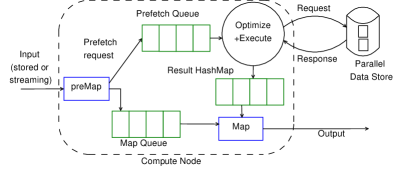
Figure 4: Invocation of preMap and Map

We extend the MapReduce API of Hadoop, map/flatMap functions of SparkRDD and the MapUpdate API of Muppet by adding preMap functions which can be used to submit prefetch requests. The user can provide an implementation of the preMap function to issue prefetch requests.

A prefetch request returns immediately after taking steps to initiate fetch of results in the background. The driver function (the function that calls the map function at the compute node) is modified so that the preMap and the map functions run as separate threads. The preMap function consumes data items from the source, issues prefetches and then adds the data items from input to a Map queue as shown in Figure 4. The compute node decides how to execute the function (at compute nodes or at data node) and sends appropriate requests to the data nodes. Once the function for a tuple is computed, it is added to a Result HashMap from where the Map function may read the computed value corresponding to the tuple read from the Map Queue.

In case of multiple joins, multiple such blocks as shown in Figure 4 can be pipelined. Instead of one $<$preMap,Map$>$ function pair, we create a series of $<$preMap,Map$>$ pairs, each to compute one join.

7.2 Batching

Sending data or compute requests individually may lead to poor performance. To improve performance, we batch multiple data fetch/prefetch or compute requests into one batch call. Details of how to implement batching without modifications to the data store are provided in Appendix D.3.

The batch size is currently decided statically, with batches kept large enough to ensure per-request overheads are small relative to the actual cost of the request. Extensions to dynamically determine batch size is a topic of future work. Note that for streaming systems a large batch size is useful to improve throughput as shown in [6]. However, batches must be kept small to keep the latency low. In order to keep the latency low, our framework allows applications to specify a maximum wait time. After the predefined amount of time has passed since the first data item was added to the queue, we send the batch irrespective of whether the batch is full or not. The waiting time to trigger a batch of requests can be adjusted depending on the latency requirements.

8 Related Work

Stream relation join: Prior work on optimization of stream-relation joins for non-distributed streaming systems includes MeshJoin [20], Semi-Streaming Index Join (SSIJ) [2], CacheJoin [18], and a technique proposed by Derakhshan et al. in [8].

However, none of these approaches consider the optimizations that we explore, such as prefetching and pushing computations to the data store. Since these techniques are not based on distributed streaming systems they also do not take into account load balancing.

Joins in distributed database systems: Tian et al. [27] considers the problem of join of HDFS data with data in enterprise data warehouses, and consider several join techniques, such as DB-Side join, HDFS-Side Broadcast join, HDFS-side repartition join, and HDFS-side zigzag join, which are based on hash joins. Indexed nested loops joins are not considered, which are key to handling streaming data, as well as in situations where the stored data size is much larger than the other join input. Further, they do not consider function executions.

Map-Side Index Nested Loop Join (MAPSIN join) [21] uses the indexing provided by HBase to perform map side joins on data stored in HBase. They do not perform any optimization when fetching data from other nodes in HBase, nor do they consider pushing computations to other nodes, or load balancing.

Skew reduction approaches: DeWitt et al. [10] address the problem of skew in parallel hash join. They use statistics to determine heavy hitters and broadcast heavy hitters from one of the join inputs, to mitigate skew, while hash partitioning the other keys. Flow-Join [23] uses approximate histograms to detect heavy-hitters from an initial part of the input relations, and then uses the broadcast/hash partition approach of [10] to mitigate skew. In particular, Flow-Join is optimized for very high bandwidth network interconnects. Neither of these techniques considers function execution costs, nor do they consider situations where the skewed keys change, as could happen in a streaming system. Furthermore, they depend on somewhat arbitrary thresholds to determine which keys are heavy hitters, whereas our approach based on ski-rental is more principled. However, our techniques have some overheads in terms of maintaining current statistics and caching. For in-memory systems with low latency network connectivity (like RDMA over InfiniBand network) and low CPU cost for function execution, the overhead of our techniques may increase the execution time, but they are useful when any of the above properties is not satisfied.

SkewReduce mitigates skew by generating partitions using static optimization techniques while SkewTune performs dynamic repartition on detecting skew, to mitigate skew across Map and Reduce sites. Unlike these techniques, our techniques can mitigate skew where the skew is caused by heavy-hitters, since the computation for a single key can be performed across multiple nodes. Our system also performs many other optimizations like batching, prefetching and frequency based caching, which other systems do not consider.

Data access optimization: The DBridge system [22] provides APIs and implementations for optimizing data accesses (e.g. using JDBC) from applications, by using batching, asynchronous invocations, and prefetching. Pyxis [3] partitions database applications into two parts, one to be run on the application server and the other at the database server, to minimize the amount of control and data flow for database calls. Both these approaches do not consider distributed systems, nor do they consider dynamic runtime load balancing. However, our implementation of batching/prefetching uses the techniques described in [22].

Load balancing: Load balancing is a well-studied topic in the context of distributed and network systems, where the goal is to distribute the incoming requests evenly among a number of nodes; see, e.g.  [25]. We instead look at balancing the function computation load between compute nodes and data nodes. Our decisions are made considering a pair of nodes at a time, but are designed to take into consideration load at other nodes as well when making the decision, to ensure overall load balance across all compute and data nodes. We are not aware of any other work which performs such optimization.

9 Experiments

For the purpose of evaluation of the efficiency of our techniques, we use our framework to optimize workloads on Hadoop YARN and Muppet, with HBase as the data store. We compare the performance of our techniques with that of existing skew mitigation techniques on an entity annotation application. For Spark, we compared the performance of our framework with SparkSQL on TPC-DS queries. We also compare the performance on synthetic workloads with different input skews for Hadoop and Muppet.

We use a cluster of 20 nodes to test the performance of our setup. Each node is equipped with two quad-core Xeon L5420 CPUs and 16 GB RAM. The amount of stored data stored in HBase was varied from 20GB to 200GB for different experiments. We limited the cache size to 100 MB in memory to consider the scenario that memory cache is not enough to store all cached items. In practice, however, data in the disk cache may actually be resident in memory as cached pages in the file-system buffer. Hence, reads from disk cache will incur file-system overhead, but may not incur actual disk access overhead, which can be very high for random IO on hard disks. Thus, our numbers would more accurately match the cost of reads from an SSD, rather than from a hard disk.

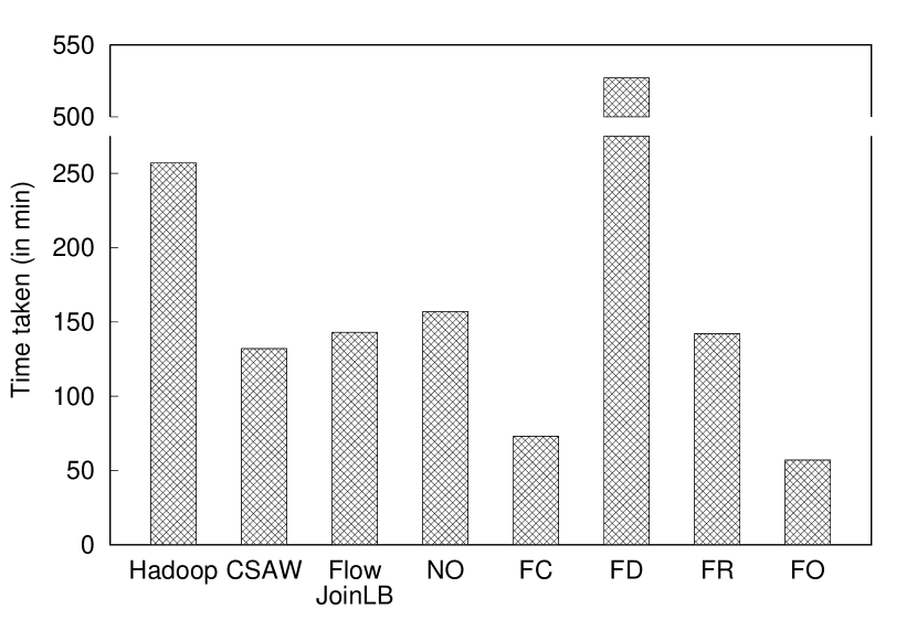
Figure 5: ClueWeb dataset entity annotation using Hadoop MapReduce

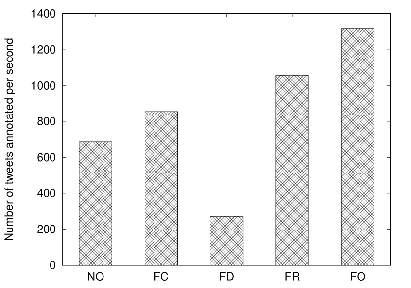
Figure 6: Twitter entity annotation using Muppet

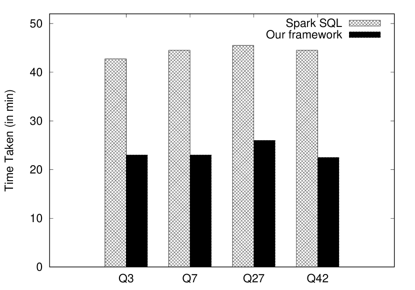
Figure 7: Multiple join TPC-DS workload on Spark, SF=500

9.1 Entity Annotation Workload

For this experiment, we compare the performance of various techniques on an implementation of entity annotation using logistic regression models. The total data size of the models 28.7 GB with the largest being 284.7 MB and the smallest is just a few bytes. Since this is highly CPU intensive even for a dataset of size 1 GB the basic MapReduce takes over 5 hours.

9.1.1 Stored Data Performance

In order to evaluate the performance of our optimizations, we compare across these options on Hadoop YARN.

• Hadoop: Basic Map Reduce in Hadoop with no skew mitigation techniques applied.

• CSAW: The technique used in [12] which estimates skew based on the frequency and the cost for annotation, and performs partitioning/replication accordingly, as discussed earlier in Section 2.1.

• FlowJoinLB: This technique uses statistics of the entire input data, and performs partitioning/replication as done in FlowJoin [23]. This technique provides a lower bound on the time taken by FlowJoin, which uses statistics based on a sample.

• NO - No Optimization: Map-side join, with data fetched using the default HBase APIs, and all function execution done at the compute nodes. None of our optimization techniques are used

• FC - Function execution at Compute nodes: Function execution is done only at the compute nodes. Techniques of batching/prefetching are used to optimize data access, but no caching of data is done.

• FD - Function execution at Data nodes: Function execution is done only at the data nodes. Techniques of batching/ prefetching are used to optimize data access. Data caching does not apply in this case.

• FR - Function execution with Random choice: The choice of compute/data request is made at random, with equal probability. Techniques of batching/ prefetching are used to optimize data access, but no caching of data is done.

• FO - Function execution Optimized: All our optimizations are used, including batching/ prefetching for optimizing data access, frequency based caching, and load balancing techniques.

We used a corpus of about 1GB/35,000 documents sampled from the ClueWeb09 dataset [4] and were able to annotate over 4.5 million entities. To run entity annotations using MapReduce, CSAW and FlowJoinLB we used all 20 nodes on the cluster, while for the rest of the techniques we used 10 nodes as data nodes (for storing data in HBase) and 10 nodes as compute nodes (for running Hadoop). Thus the total number of nodes used in the setup is same in all cases to provide a fair comparison.

We precompute statistics and cost estimates ahead of time for CSAW and FlowJoinLB and do not include the time taken. Our techniques do not need these statistics. However, all other overheads are included in the times reported.

In entity annotation, the next step is indexing which requires redistribution of tokens and entities; this incurs the same overheads for all techniques considered. However, for applications that require the annotated results to be collected with the document, our approach avoids further partitioning, since results are always fetched to the compute nodes, where the document is processed. In contrast, the other techniques would incur an extra partitioning overhead in this case.

The total amount of time taken is shown in Figure 7. A naive implementation using the Map Reduce framework causes high skew at reducers thereby creating stragglers. The straggler reducers increase the overall time taken. Similarly, for FD there was a lot of skew since some data nodes which contain heavy hitter keys or models for which classification is expensive, took much longer to complete. CSAW and FlowJoinLB reduce skew, thereby improving the performance over the naive implementation. However, we still found some skew in the time taken by the reducers.

NO and FC perform the join and classification at Map side thereby reducing skew. However, they use only 10 nodes for computation. FR spreads computations across compute and data nodes but does it at random, thus leading to skew on some data nodes. FO performs the best out of these techniques since the computation is spread uniformly across compute and data nodes due to runtime decisions made by our techniques. Note that FO takes less than half the time of CSAW, FlowJoinLB and FC takes 25% more time than FO. FC can be significantly slower for other workloads such as Twitter annotation and synthetic workloads discussed later.

One interesting issue that we observed in our framework when using Hadoop was because of tasks restarts. Some map tasks straggled a little and could not finish as fast as others. The Hadoop framework restarted these map tasks on other nodes which led to extra function calls being pushed to the HBase store thereby reducing our performance slightly. However, this did not cause any material change to our result.

9.1.2 Streaming Performance

For this experiment, we compare the performance of entity annotation, in terms of the number of tweets processed, using Muppet on a 2 GB Tweet stream from June 2016. Since Muppet is a stream processing platform, the MapReduce, CSAW and FlowJoinLB techniques do not apply. The annotator was able to identify at least one entity for annotation in about 50% of the tweets. The number of tweets processed per second across the nodes is shown in Figure 7. FC was able to annotate more tweets than NO because it used batching and prefetching. FO performed significantly better since it was able to cache frequent models and balance computations between Muppet nodes and HBase nodes, and performs almost twice as well as NO. FD performed poorly due to skew. We note that FO is only about 20% better than FR; however that difference can be significantly more with skew as shown in the ClueWeb09 dataset and synthetic workload experiments later.

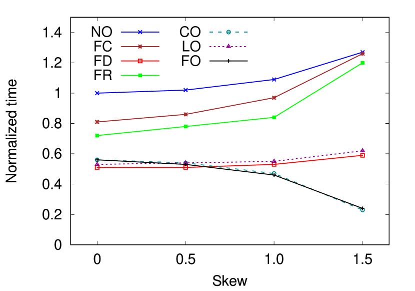
(a) Data heavy workload

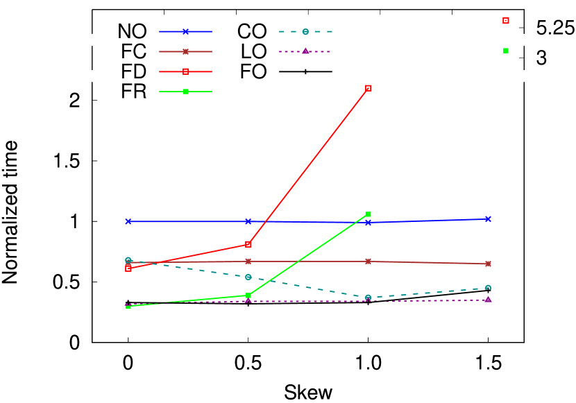
(b) Compute heavy workload

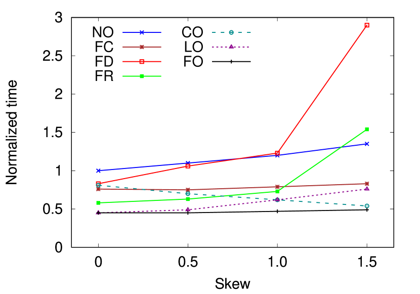
(c) Data and compute heavy workload

Figure 8: Hadoop performance comparison for synthetic workload

9.2 Multiple Joins and Spark Integration

In order to evaluate our techniques for multiple joins, we used queries from the TPC-DS benchmark to evaluate our techniques on Spark. We used a scale factor of 500 to generate the TPC-DS dataset. We selected 4 queries that joined the store_sales relation with 2 to 4 other relations.

For Spark, we used a HDFS cluster of 20 nodes to store the data and ran queries using SparkSQL which internally uses the Catalyst optimization framework to optimize queries. For our framework, we used 10 compute nodes to run Spark and 10 data nodes for HBase. The store_sales table was stored in HDFS across the 10 compute nodes and was read directly by Spark while other tables were stored in HBase. We used our extended Spark API to compute selections and joins (using the same join order as generated by Catalyst/SparkSQL) and then used SparkSQL for other operators (like aggregates, GROUP BY, ORDER BY, HAVING and LIMIT) on the join results.

The results of the experiment are shown in Figure 7. For all queries, our framework performs better since it does not need to shuffle data for computing joins.

9.3 Synthetic Workload

For this experiment, we evaluate performance on the following synthetic workloads.

• DH - Data Heavy workload: This workload computes a join and projects attributes, returning only a small result. This workload is heavy in terms of disk access and network but not on CPU. The size of data stored in HBase for this workload was 200 GB with each data fetch being about 100 KB. The total amount of data is more than the combined memory capacity of the data nodes thereby ensuring that not all data items fit into memory.

• CH - Compute Heavy workload: This workload fetches only small amount of data but performs some CPU heavy computations and simulates a compute heavy workload. Each computation takes about 100 ms on an average, while the total data size is 20 GB

• DCH - Data and Compute Heavy: This workload fetches large amounts of data as well as performs CPU intensive computations. Each computation takes about 100 ms while the dataset is 200 GB.

To distinguish the impact of caching from that of load balancing, we included the following in the performance evaluation.

• CO - Ski-Rental optimization: Ski-Rental based caching is used to find frequent items and cache them. No load balancing is used. Techniques of batching/prefetching are used to optimize data access.

• LO - Load Balancing: Load balancing techniques described in Section 5 are used to balance the load between compute and data nodes. No caching is done. Techniques of batching/prefetching are used to optimize data access.

9.3.1 Static Data Distribution

To evaluate the performance of the synthetic workloads on Hadoop YARN we compare the performance, in terms of the amount of time taken, for NO, FC, FC, FR, CO, LO and FO described earlier. We use a Zipf function to generate the join keys with different skews. We varied the skew factor, z from 0 (uniform distribution) to 1.5 (highly skewed) with steps of 0.5. Note that there is no skew in the data stored in HBase since the key is a primary key and the size of each tuple is the same. We use 10 nodes as compute nodes and 10 nodes as data nodes.

Since our experiments are on a synthetic workload, the actual time is not relevant. Hence, we normalize the time taken by fixing the time taken for the NO technique at skew 0 to be one unit of time and adjust the time taken for other techniques and skews appropriately. Across all workloads FC performs better than NO; the difference shows the benefits due to batching and prefetching optimizations.

The relative time taken for the data heavy workload is shown in Figure 8(a). For this workload, it would be beneficial to perform the join at the data node, since it would involve less network transfer cost. The performance of FO is marginally worse than FD at no skew because FO pays some overheads for cost estimation but in the end pushes compute requests to data nodes, just like FD. As the skew increases, FO caches the most frequent items and performs much better. CO and LO show the impact of the caching and load balancing components of FO. In this case, CO is identical to FO because computation load is very low, so load balancing is not useful. LO performs slightly better at low skew because it has less overheads but at higher skew CO and FO perform better because of caching.

Figure 8(b) shows the relative time taken for the compute heavy workload. At z=0, FR is able to evenly distribute the compute load between the compute and data nodes and hence performs very well. However, with increase in skew FR sends many compute requests to data nodes with skewed keys, and the performance falls. Similarly, for FD the time taken increases with increase in skew because some data nodes get very heavily loaded. At z=0, CO sends all computations to the data nodes and performs similar to FR. At higher skew CO is able to cache skewed values at compute nodes and offload some computations from the data nodes. However, LO and FO are able to better balance the computations between the compute and data nodes at all skews and hence outperform CO. At skew of z=1.5, the performance of FO decreases slightly since most of the computations are performed on cached items and our techniques perform the computation for cached items at compute nodes, leaving data nodes under utilized; LO, which does not cache data, is able to balance the load slightly better. Extending our load balancing techniques to detect and handle such execution skew is a topic of future work.

The relative time taken for the compute and data heavy workload is shown in Figure 8(c). For this workload, FO outperforms FR even at z=0 because it balances between compute and data requests in a cost based manner, taking into account both the compute and data costs, while FR sends requests randomly. Similar to the compute heavy workload, as skew increases performance of FR reduces because it overloads some data nodes with too many requests. At low skew, CO is not able to cache values and hence sends all computations to the data nodes. However, with increase in skew CO is able to cache values for skewed keys and performs some computations at the compute nodes and hence its performance increases. LO does not do any caching and at high skew it needs to fetch a lot of data from data nodes that contain higher skewed values. Hence, its performance decreases with increase in skew. FO works well across all skew values.

We also ran this experiment on the Muppet stream processing system. Results are presented in Appendix D. The performance benefit of the optimizations for Muppet on these workloads is very similar to that of Hadoop. Across the board, FO performs best or close to the best.

9.3.2 Dynamic Data Distribution

To evaluate our performance for changing distribution, we conducted another experiment with synthetic workloads where we dynamically changed the distribution. For each skew value, we changed the frequent keys 10 times during our experiment.

For the first set of experiments, we compared the performance of the earlier mentioned techniques on the dataset with changing distribution. We did not observe any noticeable difference and the results were similar to the one shown in Figure 8.

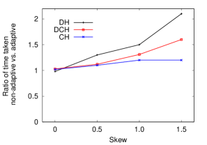
Figure 9: Adaptive vs non-adaptive optimization with load balancing

For the second set of experiments, we compare the performance of FO, which adapts continuously, with that of non-adaptive optimization. For non-adaptive optimization, ski-rental based caching decisions are made for only the first 10% of the tuples and the cache contents are not changed subsequently. Load balancing was performed as before.

Figure 9 shows the ratio of the time taken by the non-adaptive technique to that of the adaptive technique for the data heavy (DH), compute heavy (CH) and the data and compute heavy (DCH) workloads. When there is no skew (i.e., uniform distribution), the adaptive and non-adaptive techniques work equally well. For the compute heavy workload, CH the non-adaptive technique is able to balance the load among data and compute nodes and hence adaptive performs only slightly better. For DH and DCH, which benefit more from caching frequent values, the adaptive technique performs significantly better than the non-adaptive technique.

10 Conclusion

In this paper, we looked at techniques to optimize remote data access and function invocations by optimizing the location of function execution using ski-rental based caching and load-balancing techniques, along with prefetching and batching optimizations for applications running on parallel data frameworks. Our performance results show significant benefits in terms of throughput improvement across different frameworks and workloads. Our techniques can also be used for optimization of joins, with optional UDFs, in parallel databases.

Areas of future work include dynamic choice of batch size and batch timeout taking latency into account, handling user defined functions with side effects and elastically increasing or decreasing compute nodes based on load. Another area of future work is to extend the Catalyst optimizer of SparkSQL to use our join technique when appropriate.

Appendix A Other Application Domains

CloudBurst [24] aligns a (large) set of genome sequence reads (which are typically small) with a reference genome sequence, to find locations in the reference sequence that approximately match each read. CloudBurst is implemented using MapReduce. One map function extracts n-grams from the reads, and outputs (n-gram, string) pairs, with the n-gram as the key for the reduce phase. A similar map function extracts n-grams from the reference sequence, and outputs (n-gram, string) pairs. The reducer for a particular n-gram matches each read with the reference sequence string at the matching location using approximate matching algorithms. As pointed in [14], the basic MapReduce implementation leads to skew, with one of the important causes being a variance in cost of user defined operations (UDOs) executed at the reducers (UDOs correspond to UDFs in our framework). The SkewTune technique of [14] detects skew and repartitions tasks assigned to straggler reducers, to mitigate skew.

The reduce function in CloudBurst basically performs a join, followed by a UDF computation. Our framework could be used to handle this problem as follows. The reads are partitioned amongst compute nodes. The n-grams from the reference sequence are computed and indexed with the n-grams as keys, and the strings around the n-gram location as values. The map function extracts n-grams from the reads, and for each n-gram, fetches matching reference strings from the datastore. The approximate matching is done as a UDF. Note that if the join is done at the reducer, all reads with a particular n-gram would go to a single reducer; whereas in our case the join can be performed at the map-side, and these n-grams thus get distributed across multiple compute nodes, evening out the UDF load. Note that unlike SkewTune, our techniques are applicable to streaming systems also.

As mentioned in [14] there are many MapReduce applications that use UDOs and suffer from skew. We do not have details of the applications, but we believe our techniques would be applicable to at least some of them.

Appendix B Managing Memory & Disk Caches

As discussed in Section 4.2.2, the condCacheInMemory function is used to determine if a data item is to be cached in memory or disk. We describe this function in detail in this section. We first consider the simpler case where all data items are the same size, and then consider the general case where data items can be of different sizes.

We denote the memory cache as mCache, and the disk cache as dCache and their respective sizes be $s_{m}$ and $s_{d}$.

B.1 Uniform data item caching

The condCacheInMemory for the case where data items are of uniform sizes is described in Algorithm 2. Given a new data item, this function checks if it is to be cached in memory or not. If the free space in cache is more than the size of the item, it is added to cache. If not, the algorithm compares the benefit of the new data item and the item with the lowest benefit in mCache. If the benefit of the new data item is higher, the item with the lowest benefit in mCache is moved to disk cache, and the current data item is cached in memory. In both the above cases the function returns TRUE otherwise, it returns FALSE.

Note that we assume that the disk cache is large enough to cache all fetched items. In case the disk cache is full, items from disk cache with low benefit could be evicted from dCache in order to accommodate items with a higher benefit. Also, data items that are moved to mCache in the function condCacheInMemory could be removed from dCache to save space in the disk cache (although there would be a cost to moving it back to disk in case it is evicted from memory).

B.2 Non-uniform data item caching

In case the size of data items is variable, we use Algorithm 3 to check whether to put an item in mCache. Unlike the fixed size case, removing one item from mCache may not create sufficient free space to add a new item. We, therefore, find $i$ items with the least priority such that eliminating these items would free up enough space to add the new item to mCache. If the sum of priorities of the items to be evicted is less than the priority of the new data item, we return FALSE. Note that since we chose the items in increasing order of benefit until there was enough space, it is possible that some subset of them may actually suffice to create enough space for the new item. We, therefore, pick items with the most benefit that can be retained, while freeing up enough space for the new item. The remaining items are evicted to disk, and add the new item is added to mCache.

0:  k = key to be updated, v = value of item, s = size of item

1:  if mCache.freeMem $\geq$ s then

2:     mCache.add(k,v)

3:     return  TRUE

4:  else if benefit(k) $>$ mCache.minBenefit then

5:     minPE $\leftarrow$ mCache.minBenefitElement

6:     mCache.remove(minPE)

7:     memCache.add(k,v)

8:     if minP $\notin$ dCache then

9:        dCache.add(minPE)

10:     end if

11:     return  TRUE

12:  else

13:     return  FALSE

14:  end if

Algorithm 2 : condCacheInMemory
(with uniform item size)

Note that after the above step, there may be some free space in mCache. We do not actively pull elements from disk cache to fill up the free space. Instead, we fill the free space lazily when other items are accessed.

Note that as for the fixed item size case, we assume that disk cache is unlimited. In case the disk cache size is limited, items from disk cache with low benefit to size ratio could be evicted from disk cache in order to accommodate items with higher benefit to size ratio.

0:  k = key to be updated, v = value of item, s = size of item

1:  if mCache.freeMem $\geq$ s then

2:     mCache.add(k,v)

3:     return  TRUE

4:  else

5:     prelimList $\leftarrow$ i items with least benefits $\mid$ $\sum$size + mCache.freeMem$>$ s

6:     freeMem $\leftarrow$ mCache.freeMem+ $\sum_{i}$ preimList(i)

7:     if $benefit(k)\geq\sum$ benefit(prelimList) then

8:        keepList $\leftarrow$ items in prelimList with most benefit $\mid$ size(keepList) $\leq$ freeMem$-$s

9:        removeList $\leftarrow$ prelimList - keepList

10:        for item $\in$ removeList do

11:           mCache.remove(item)

12:           if item $\notin$ dCache then

13:              dCache.add(item)

14:           end if

15:        end for

16:        mCache.add(k,v)

17:        return  TRUE

18:     else

19:        return  FALSE

20:     end if

21:  end if

Algorithm 3 : condCacheInMemory
(with variable size items)

Appendix C Load computation

In Section 5, we discussed how on receiving a request batch from a compute node, a data node balances the load between itself and the compute node by estimating its own load and the load at compute and then deciding to compute only a fraction of requests from the batch locally. We now discuss how a data node estimates load, based on the statistics sent to it from compute nodes and statistics available locally.

Consider a batch of $b$ requests sent from the compute node $i$ to the data node $j$. The data node chooses to compute $d$ requests at the data node itself and send $b-d$ computations back at the compute node.

The load at compute node $i$ at a point in time is estimated based on the following parameters, which are measured continuously at runtime. (Parameters sent from the compute node are marked with superscript $c$ while those computed at the data node are marked with superscript $d$.)

• $lc^{c}_{i}$: number of pending local computations (based on fetched values) at compute node $i$

• $nd^{c}_{i}$: number of pending data requests to be sent from compute node $i$

• $nc^{c}_{i}$: number of pending compute requests to be sent from compute node $i$

• $ndr^{c}_{i}$: number of pending responses to data requests sent from compute node $i$

• $\overline{nr}^{c}_{ij}$: total number of pending compute requests at compute node $i$ across data nodes other than $j$

• $\overline{r}^{c}_{ij}$: number of pending compute requests at compute node $i$ expected to be computed at the data nodes other than $j$ (this is computed based on recent history)

• $nr^{d}_{ij}$: number of pending compute requests sent to data node $j$ from compute node $i$

• $r^{d}_{ij}$: number of pending compute requests sent to the data node $j$ from the compute node $i$ that are to be computed at the $j$

The load at a data node $j$ can be estimated using the following parameters.

• $nd^{c}_{j}$: number of data requests pending at data node $j$ from all compute nodes

• $ndr^{d}_{j}$: number of pending data request responses to be send from data node $j$

• $nr^{d}_{j}$: total number of pending compute requests (from all compute nodes) at data node $j$ (note that some of these may be sent back to the compute nodes)

• $r^{d}_{j}$: number of pending compute requests (from all compute nodes) to be computed at the data node

• $nr_{ij}^{d}$: the number of pending compute requests at data node $j$ from compute node $i$

• $r_{ij}^{d}$: number of pending compute requests from the compute node $i$ to be computed at the data node $j$

Let the time taken to compute the function at compute node be $tc^{c}$ while the time taken to compute a function at data node be $tc^{d}$. Let the size of the key be $s_{k}$, the size of the parameters be $s_{p}$, the size of the store value be $s_{v}$ and the size of the computed value be $s_{cv}$. The load is estimated in terms of CPU and network as shown below.

The CPU load at compute node $i$ is the time taken for computation of (1) the number of pending computations to be performed at $i$ ($lc^{c}_{i}$), (2) the estimated number of computations that are returned from the data nodes other than $j$ (these estimates are based on recent history) ($\overline{nr}^{c}_{ij}-\overline{r}^{c}_{ij}$), (3) the number of computations that are to be returned from $j$ to $i$ from previous requests pending at $j$ ($nr^{d}_{ij}-r^{d}_{ij}$) and (4) the number of requests, for the current batch, that are to be computed at $i$, i.e. $b-d$. Hence, the CPU load at compute node $i$ can be estimated as

$$compCPU(d)=tc^{c}*lc^{c}_{i}+tc^{d}*(\overline{nr}^{c}_{ij}-\overline{r}^{c}_{ij})$$

$$+tc^{d}*(nr^{d}_{ij}-r^{d}_{ij})+tc^{d}*(b-d)$$

Similarly the CPU load at data node $j$ can be estimated as

$$dataCPU(d)=tc^{d}*r^{d}_{j}+tc^{d}*d$$

The time taken for network communication for a node is $networkLoad/netBw$. The network load at the compute node $i$ is the sum (1) the number of pending data and compute requests to be sent from compute node $i$ to data nodes ($nd^{c}_{i}$ and $nc^{c}_{i}$ respectively), (2) the number of pending responses to data requests sent from $i$ ($ndr^{c}_{i}$), (3) the estimated number of computed and uncomputed responses to compute requests made by $i$ to data nodes other than $j$ ($\overline{r}^{c}_{ij}$ and $\overline{nr}^{c}_{ij}-\overline{r}^{c}_{ij}$ respectively), (4) the number of computed and uncomputed responses to compute requests to $j$ for previous requests (${r}^{d}_{ij}$ and ${nr}^{d}_{ij}-{r}^{d}_{ij}$ respectively), and (5) the number of computed and uncomputed responses for the current batch of requests ($d$ and $b-d$ respectively). Thus the network load at the compute node $i$, is a function can be computed as

$compNet(d)=$

$$\frac{\displaystyle\begin{multlined}nd^{c}_{i}*(s_{k}+s_{v})+nc^{c}_{i}*(s_{k}+s_{p})+ndr^{c}_{j}*s_{v}\\ \displaystyle\begin{multlined}+(\overline{nr}^{c}_{ij}-\overline{r}^{c}_{ij})*s_{v}+\overline{r}^{c}_{ij}*s_{cv}\\ \begin{multlined}+({nr}^{d}_{ij}-{r}^{d}_{ij})*s_{v}+{r}^{d}_{ij}*s_{cv}\\ +d*s_{cv}+(b-d)*s_{v}\end{multlined}+({nr}^{d}_{ij}-{r}^{d}_{ij})*s_{v}+{r}^{d}_{ij}*s_{cv}\\ +d*s_{cv}+(b-d)*s_{v}\end{multlined}+(\overline{nr}^{c}_{ij}-\overline{r}^{c}_{ij})*s_{v}+\overline{r}^{c}_{ij}*s_{cv}\\ \begin{multlined}+({nr}^{d}_{ij}-{r}^{d}_{ij})*s_{v}+{r}^{d}_{ij}*s_{cv}\\ +d*s_{cv}+(b-d)*s_{v}\end{multlined}+({nr}^{d}_{ij}-{r}^{d}_{ij})*s_{v}+{r}^{d}_{ij}*s_{cv}\\ +d*s_{cv}+(b-d)*s_{v}\end{multlined}nd^{c}_{i}*(s_{k}+s_{v})+nc^{c}_{i}*(s_{k}+s_{p})+ndr^{c}_{j}*s_{v}\\ \displaystyle\begin{multlined}+(\overline{nr}^{c}_{ij}-\overline{r}^{c}_{ij})*s_{v}+\overline{r}^{c}_{ij}*s_{cv}\\ \begin{multlined}+({nr}^{d}_{ij}-{r}^{d}_{ij})*s_{v}+{r}^{d}_{ij}*s_{cv}\\ +d*s_{cv}+(b-d)*s_{v}\end{multlined}+({nr}^{d}_{ij}-{r}^{d}_{ij})*s_{v}+{r}^{d}_{ij}*s_{cv}\\ +d*s_{cv}+(b-d)*s_{v}\end{multlined}+(\overline{nr}^{c}_{ij}-\overline{r}^{c}_{ij})*s_{v}+\overline{r}^{c}_{ij}*s_{cv}\\ \begin{multlined}+({nr}^{d}_{ij}-{r}^{d}_{ij})*s_{v}+{r}^{d}_{ij}*s_{cv}\\ +d*s_{cv}+(b-d)*s_{v}\end{multlined}+({nr}^{d}_{ij}-{r}^{d}_{ij})*s_{v}+{r}^{d}_{ij}*s_{cv}\\ +d*s_{cv}+(b-d)*s_{v}}{netBw_{i}}$$

Similarly, the network load at data node $j$ is a function of $r_{j}$,

$dataNet(d)=$

$$\dfrac{\displaystyle\begin{multlined}nd^{c}_{j}*(s_{k}+s_{v})+ndr^{d}_{j}*s_{v}+nr^{d}_{j}*(s_{k}+s_{p})\\ \begin{multlined}+(nr^{d}_{j}-r^{d}_{j})*s_{v}+r^{d}_{j}*s_{cv}\\ +d*s_{cv}+(b-d)*s_{v}\end{multlined}+(nr^{d}_{j}-r^{d}_{j})*s_{v}+r^{d}_{j}*s_{cv}\\ +d*s_{cv}+(b-d)*s_{v}\end{multlined}nd^{c}_{j}*(s_{k}+s_{v})+ndr^{d}_{j}*s_{v}+nr^{d}_{j}*(s_{k}+s_{p})\\ \begin{multlined}+(nr^{d}_{j}-r^{d}_{j})*s_{v}+r^{d}_{j}*s_{cv}\\ +d*s_{cv}+(b-d)*s_{v}\end{multlined}+(nr^{d}_{j}-r^{d}_{j})*s_{v}+r^{d}_{j}*s_{cv}\\ +d*s_{cv}+(b-d)*s_{v}}{netBw_{j}}$$

As described in Section 5 we need to choose $d$ that minimizes the maximum of the four loads described above. All the functions are linear in d. The choice of $d$ needs to be made for each batch of compute request. We use gradient descent as a cheap heuristic to compute d even though it does not guarantee a global minimum and may get stuck at a local minimum. The gradient descent initially starts with a random point, $\bar{d}$ between $0$ and $b$ which gives us an initial value for the max function. We then iteratively follow the decreasing slope till we get a minimum.

Appendix D Implementation

In this section, we describe our cache implementation as well as our implementation of preMap for Hadoop MapReduce and Muppet stream processing framework. We also describe how we use batch compute requests for HBase and measure network bandwidth.

preMap(docId,document) {
  for each spot in document.getSpots() {
   spotContext =
        getContextRecord(spot, document)
   submitComp(f,spotContext.key,spotContext.value)
  }
  mapQueue.add([docId,document])
}

map(docId,document)
  for each spot in document.getSpots() {
    spotContext = getContextRecord(spot, document)
    annotatedValues =
     fetchComp(f,spotContext.key,spotContext.value)
    context.write(annotatedValues)
  }
}
ΨΨ
f(key, params){
  model = getModel(key)
  annotatedValues = classifyRecord(params, model)
  return annotatedValues
}

Figure 10: Entity annotation using prefetching

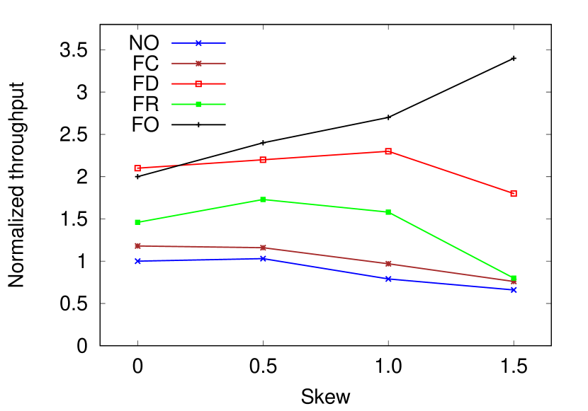
(a) Data heavy workload

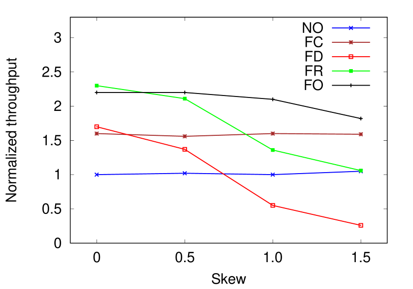
(b) Compute heavy workload

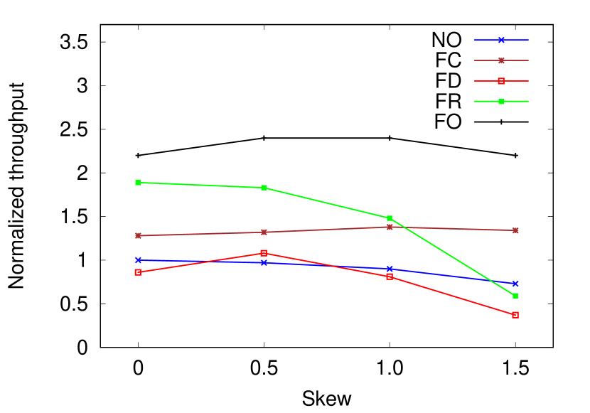
(c) Data and compute heavy workload

Figure 11: Muppet throughput comparison

D.1 Cache Implementation

We use the Ehcache [11] library for our cache implementation. Ehcache provides APIs for defining a composite cache that can be partially kept in memory and partially on disk. Users can also define the size of cache for the memory and disk components. We define our own eviction policy, for evicting cached items from memory, to disk cache by extending the AbractPolicy class provided by Ehcahe.

As mentioned earlier, data in the disk cache may actually be resident in memory as cached pages in the file-system buffer. Hence, reads from disk cache will incur file-system overhead, but may not incur actual disk access overhead, which can be very high for random I/O on hard disks.

D.2 Implementation of preMap

As described in Section 7, we have extended the Hadoop MapReduce, Spark and Muppet APIs to allow the user to write a preMap function that can issue prefetch requests.

To illustrate the use of the API we modify the entity annotation program in Figure 3. The program using prefetching is shown in Figure 10. The submitComp function is a prefetch call that internally adds a $(f,p,k)$ data item to a Prefetch queue and returns. Process threads read data from the queue and an optimizer module decides whether to issue a data request or compute requests. Depending on the type of request the data item is added to corresponding data or compute queues. Once the function is computed (either at the data node or the compute node) the result is added to the resultHashMap and can then be used later in map function.

The map function is then called on values from the queue and performs a blocking fetch using fetchComp. If the value (data item or compute request) from the data node has already been fetched, it can be processed immediately; otherwise the compute node waits till the values become available. The exact way in which the preMap function is invoked depends on the system on which it is implemented.

The invocation of preMap function for different systems is implemented as follows

• Hadoop: The Hadoop Mapper class uses a setup function to initialize the Mapper and a run function to read input and call the map function. We modify the setup function in the Mapper class to start a new thread, from which the preMap function is called on each input data item. The user code implementing the preMap function can issue prefetch requests from the data store. Once the input data item is processed by preMap, it is added to a MapInput queue that we create. The run function in the Mapper is modified to read values from the MapInput queue (instead of directly from the input), and it then calls the map function.

• Spark: In Spark, map or flatMap functions may be used to operate on RDDs similar to the map function in Hadoop. The user can create functions that need to be called for flatMap or map. We extend the Spark RDD to include additional functions flatMapWithPremap and mapWithPremap. The parameters to flatMapWithPremap and mapWithPremap are two user defined functions (wrapped in a class). The user defined class implements the call(t, asyc) function, to define how the input tuple t will be processed. The async object can be used to submit prefetch requests in preMap or retrieve results in mapWithPremap/flatMapWithPremap.

• Muppet: In the Muppet stream processing framework, the MapUpdatePool class reads values from the input stream and adds it to a Map queue for processing. We extend the framework by creating a new thread in the constructor of MapUpdatePool for prefetching. The prefetching thread reads the input from the stream, adds it to a prefetch queue and adds the tuples to the Map queue in MapUpdatePool. Another thread reads values from the prefetch queue and issues prefetches.

Some preprocessing on the raw input data may be needed to decide what data items are to be prefetched. This processing would be repeated at the map function also. In the entity annotation example shown in Figure 10, the spots = document.getSpots needs to be repeated. As an optimization, we implement another extension where the prefetch thread provides the preprocessed data to be consumed by a postMap function instead. The user can provide implementations for preMap and postMap.

D.3 Compute Request Implementation

We have implemented libraries for the optimizations described in this paper in Java, with Apache HBase as the datastore. We use the endpoint coprocessor in HBase to perform computations at the data nodes.

Note that invocations to the data store need to be done for batches of requests, rather than for individual requests. This can be done by creating a batched form of the function, which takes a set of requests instead of a single request. The decision on what to compute and what to return as data is made by the batched version of the function. Thus, no changes need to be made to the data store.

HBase stores tabular data partitioned into regions. Each data node may have one or more regions. Coprocessor calls to the HBase need to define a start key, an end key, the table name on which the coprocessor will be invoked and the coprocessor class. The HBase API sends the request parameters to each region that has keys in the range [startKey,endKey] and invokes the function calls on that region. The results obtained from each region are then accumulated by the caller.

Since HBase provides API to get the data node for each key, at each compute node we maintain one batch of requests for each data node. Once the batch for a data node fills up, we send the batched request to the data node using coprocessor execution calls.

In our coprocessor calls, we need to pass the $(k_{i},p_{i})$ pairs along with the necessary statistics as request parameters. In case there are $r$ regions at one data node all the $(k_{i},p_{i})$ pairs will need to be sent $r$ times (once for each region) if the default HBase API is used. We instead provide a wrapper API which takes input $(k_{i},p_{i})$ pairs, the table name and the coprocessor class. Our API sends requests to regions such that only the $(k_{i},p_{i})$ pairs for which $k_{i}$ is in the range of a region are sent to that region.

D.4 Bandwidth Estimation

To measure the effective network bandwidth available for each compute node and data node, we send data packets from all the compute nodes to all the data nodes and vice versa and measure the time taken under load. $netBw_{i}$ is the aggregate of the network bandwidth at node $i$. Bandwidth estimation is done once during the initial setup and the value of bandwidth is used for optimizations computations. The network bandwidth measurement step allows our framework to be used even if the bandwidth to some nodes (e.g. intra-rack bandwidth) is different from the bandwidth to others (e.g. inter-rack bandwidth). In this case, we compute the average bandwidth across all destinations, reflecting the fact that communication will be distributed across all the destinations.

In the case of a dedicated network, the bandwidth will not change during a computation except due to failures. However, in a shared infrastructure, bandwidth may change. To the best of our knowledge, there is no non-intrusive method to measure network bandwidth while the functions are running. Any attempt to measure bandwidth by sending additional packets will reduce the performance of the program, while measuring rate of arrival of requests/results will not be able to separate the network bandwidth from processing bandwidth. However, if desired the network bandwidth can be measured and updated at runtime at the cost of affecting performance temporarily, and we can use the updated bandwidth in our computations.

Appendix E Synthetic Workload Muppet

For Muppet we compare the performance, in terms of the throughput (number of input tuples processed per unit time), for NO, FC, FC, FR and FO. We consider the throughput to be one tuple per unit time for NO technique and normalize throughput for other techniques and skews. For the results of these experiments, higher numbers indicate better performance.

The normalized throughput for data heavy workload is shown in Figure 11(a). The throughput of FD is comparable to that of FO at z=0 but the throughput of FD decreases with skew because some data nodes process a lot of requests, while the throughput of FO increases because of caching. Similarly, the performance of NO,FC and FR decrease with increase in skew. For this workload as well as the other workloads, FC performs better than NO because of prefetching/batching optimizations.

The normalized throughput for compute heavy workload is shown in Figure 11(b). FR performs better than FO at less load, but throughput of FR reduces significantly with increase in skew because a few data nodes do most of the computations. FO provides the best performance at higher skew. As with MapReduce the performance of FO decreases with increase in skew since most requests are for data items already in cache and hence function computation is done locally; the data nodes remain underutilized.

The normalized throughput for the compute and data heavy combined workload is shown in Figure 11(c). For this workload, FO performs better than other workload at all skews since it can balance the CPU and network loads and cases frequent items.

References

- [1] M. Arlitt, L. Cherkasova, J. Dilley, R. Friedrich, and T. Jin. Evaluating content management techniques for web proxy caches. SIGMETRICS Perform. Eval. Rev., 27(4), Mar. 2000.
- [2] M. A. Bornea, A. Deligiannakis, Y. Kotidis, and V. Vassalos. Semi-streamed index join for near-real time execution of ETL transformations. In ICDE, pages 159–170, 2011.
- [3] A. Cheung, S. Madden, O. Arden, and A. C. Myers. Automatic partitioning of database applications. Procs. VLDB, 5(11):1471–1482, 2012.
- [4] The ClueWeb09 dataset. http://lemurproject.org/clueweb09.
- [5] G. Cormode and M. Hadjieleftheriou. Finding the frequent items in streams of data. Commun. ACM, 52(10):97–105, Oct. 2009.
- [6] T. Das, Y. Zhong, I. Stoica, and S. Shenker. Adaptive stream processing using dynamic batch sizing. In ACM SoCC, pages 1–13, 2014.
- [7] A. Davis, A. Veloso, A. S. da Silva, W. Meira, Jr., and A. H. F. Laender. Named entity disambiguation in streaming data. In ACL ’12, pages 815–824, 2012.
- [8] R. Derakhshan, A. Sattar, and B. Stantic. A new operator for efficient stream-relation join processing in data streaming engines. In CIKM, pages 793–798, 2013.
- [9] A. Deshpande and J. M. Hellerstein. Lifting the burden of history from adaptive query processing. In VLDB, pages 948–959, 2004.
- [10] D. J. DeWitt, J. F. Naughton, D. A. Schneider, and S. Seshadri. Practical skew handling in parallel joins. In VLDB, pages 27–40, 1992.
- [11] Ehcache. http://www.ehcache.org.
- [12] S. Gupta, V. Chandramouli, and S. Chakrabarti. Web-scale entity annotation using mapreduce. In HiPC, pages 99–108, 2013.
- [13] A. R. Karlin, M. S. Manasse, L. Rudolph, and D. D. Sleator. Competitive snoopy caching. Algorithmica, 3(1-4):79–119, 1988.
- [14] Y. Kwon, K. Ren, M. Balazinska, and B. Howe. Managing skew in hadoop. IEEE DATA ENG. BULL., VOL, 2013.
- [15] W. Lam, L. Liu, S. Prasad, A. Rajaraman, Z. Vacheri, and A. Doan. Muppet: Mapreduce-style processing of fast data. Procs. VLDB, 5(12):1814–1825, 2012.
- [16] M. Li, D. G. Andersen, J. W. Park, A. J. Smola, A. Ahmed, V. Josifovski, J. Long, E. J. Shekita, and B.-Y. Su. Scaling distributed machine learning with the parameter server. In OSDI, 2014.
- [17] G. S. Manku and R. Motwani. Approximate frequency counts over data streams. In VLDB, pages 346–357, 2002.
- [18] M. A. Naeem, G. Dobbie, and G. Weber. A lightweight stream-based join with limited resource consumption. In DaWaK, pages 431–442, 2012.
- [19] S. Podlipnig and L. Böszörmenyi. A survey of web cache replacement strategies. ACM Comput. Surv., 35(4):374–398, Dec. 2003.
- [20] N. Polyzotis, S. Skiadopoulos, P. Vassiliadis, A. Simitsis, and N. E. Frantzell. Supporting streaming updates in an active data warehouse. In ICDE, 2007.
- [21] M. Przyjaciel-Zablocki, A. Schätzle, T. Hornung, C. Dorner, and G. Lausen. Cascading map-side joins over HBase for scalable join processing. SSWS+HPCSW, 2012.
- [22] K. Ramachandra, M. Chavan, R. Guravannavar, and S. Sudarshan. Program transformations for asynchronous and batched query submission. IEEE TKDE, 27(2):531–544, 2015.
- [23] W. Rödiger, S. Idicula, A. Kemper, and T. Neumann. Flow-join: Adaptive skew handling for distributed joins over high-speed networks. In ICDE, 2016.
- [24] M. C. Schatz. Cloudburst. Bioinformatics, 25(11), June 2009.
- [25] N. G. Shivaratri, P. Krueger, and M. Singhal. Load distributing for locally distributed systems. IEEE Computer, 25(12), Dec. 1992.
- [26] A. Smola and S. Narayanamurthy. An architecture for parallel topic models. Proc. VLDB Endow., 3(1-2), Sept. 2010.
- [27] Y. Tian, T. Zou, F. Ozcan, R. Goncalves, and H. Pirahesh. Joins for hybrid warehouses: Exploiting massive parallelism in hadoop and enterprise data warehouses. In EDBT, pages 373–384, 2015.
- [28] A. Toshniwal, S. Taneja, A. Shukla, K. Ramasamy, J. M. Patel, S. Kulkarni, J. Jackson, K. Gade, M. Fu, J. Donham, N. Bhagat, S. Mittal, and D. V. Ryaboy. Storm@twitter. In SIGMOD, pages 147–156, 2014.
- [29] M. Zaharia, M. Chowdhury, M. J. Franklin, S. Shenker, and I. Stoica. Spark: cluster computing with working sets. In HotCloud, 2010.