Differentially Private Bayesian Learning on Distributed Data

Abstract

Many applications of machine learning, for example in health care, would benefit from methods that can guarantee privacy of data subjects. Differential privacy (DP) has become established as a standard for protecting learning results. The standard DP algorithms require a single trusted party to have access to the entire data, which is a clear weakness. We consider DP Bayesian learning in a distributed setting, where each party only holds a single sample or a few samples of the data. We propose a learning strategy based on a secure multi-party sum function for aggregating summaries from data holders and the Gaussian mechanism for DP. Our method builds on an asymptotically optimal and practically efficient DP Bayesian inference with rapidly diminishing extra cost.

1 Introduction

Differential privacy (DP) [10, 12] has recently gained popularity as the theoretically best-founded means of protecting the privacy of data subjects in machine learning. It provides rigorous guarantees against breaches of individual privacy that are robust even against attackers with access to additional side information. DP learning methods have been proposed e.g. for maximum likelihood estimation [25], empirical risk minimisation [5] and Bayesian inference [e.g. 8, 14, 17, 18, 20, 26, 30]. There are DP versions of most popular machine learning methods including linear regression [17, 29], logistic regression [4], support vector machines [5], and deep learning [1].

Almost all existing DP machine learning methods assume that some trusted party has unrestricted access to all data in order to add the necessary amount of noise needed for the privacy guarantees. This is a highly restrictive assumption for many applications and creates huge privacy risks through a potential single point of failure.

In this paper we introduce a general strategy for DP Bayesian learning in the distributed setting with minimal overhead. Our method builds on the asymptotically optimal sufficient statistic perturbation mechanism [14, 17] and shares its asymptotic optimality. The method is based on a DP secure multi-party communication (SMC) algorithm, called Distributed Compute algorithm (DCA), for achieving DP in the distributed setting. We demonstrate good performance of the method on DP Bayesian inference using linear regression as an example.

2 Our contribution

We propose a general approach for privacy-sensitive learning in the distributed setting. Our approach combines SMC with DP Bayesian learning methods, originally introduced for the trusted aggregator setting, to achieve DP Bayesian learning in the distributed setting.

To demonstrate our framework in practice, we combine the Gaussian mechanism for $(\epsilon,\delta)$-DP with efficient DP Bayesian inference using sufficient statistics perturbation (SSP) and an efficient SMC approach for secure distributed computation of the required sums of sufficient statistics. We prove that the Gaussian SSP is an efficient $(\epsilon,\delta)$-DP Bayesian inference method and that the distributed version approaches this quickly as the number of parties increases. We also address the subtle challenge of normalising the data privately in a distributed manner, required for the proof of DP in distributed DP learning.

3 Background

3.1 Differential privacy

Differential privacy (DP) [12] gives strict, mathematically rigorous guarantees against intrusions on individual privacy. A randomised algorithm is differentially private (DP) if its results on adjacent data sets are likely to be similar. Here adjacency means that the data sets differ by a single element, i.e., the two data sets have the same number of samples, but they differ on a single one. In this work we utilise a relaxed version of DP called $(\epsilon,\delta)$-DP [10, Definition 2.4].

Definition 3.1.

A randomised algorithm $\mathcal{A}$ is $(\epsilon,\delta)$-DP, if for all $\mathcal{S}\subseteq$ Range $(\mathcal{A})$ and all adjacent data sets $D,D^{\prime}$,

$$P(\mathcal{A}(D)\in\mathcal{S})\leq\exp(\epsilon)P(\mathcal{A}(D^{\prime})\in\mathcal{S})+\delta.$$

The parameters $\epsilon$ and $\delta$ in Definition 3.1 control the privacy guarantee: $\epsilon$ tunes the amount of privacy (smaller $\epsilon$ means stricter privacy), while $\delta$ can be interpreted as the proportion of probability space where the privacy guarantee may break down.

There are several established mechanisms for ensuring DP. We use the Gaussian mechanism [10, Theorem 3.22]. The theorem says that given a numeric query $f$ with $l_{2}$-sensitivity $\Delta_{2}(f)$, adding noise distributed as $N(0,\sigma^{2})$ to each output component guarantees DP, when

$$\sigma^{2}>2\ln(1.25/\delta)(\Delta_{2}(f)/\epsilon)^{2}.$$ (1)

Here, the $l_{2}$-sensitivity of a function $f$ is defined as

$$\Delta_{2}(f)=\underset{\underset{||D-D^{\prime}||_{1}=1}{D,D^{\prime}}}{\sup}||f(D)-f(D^{\prime})||_{2}.$$ (2)

3.2 Differentially private Bayesian learning

Bayesian learning provides a natural complement to DP because it inherently can handle uncertainty, including uncertainty introduced to ensure DP [27], and it provides a flexible framework for data modelling.

Three distinct types of mechanisms for DP Bayesian inference have been proposed:

1. Drawing a small number of samples from the posterior or an annealed posterior [9, 26];

2. Sufficient statistics perturbation (SSP) of an exponential family model [14, 17, 20]; and

3. Perturbing the gradients in gradient-based MCMC [26] or optimisation in variational inference [18].

For models where it applies, the SSP approach is asymptotically efficient [14, 17], unlike the posterior sampling mechanisms. The efficiency proof of [17] can be generalised to $(\epsilon,\delta)$-DP and Gaussian SSP as shown in the Supplementary Material.

The SSP (#2) and gradient perturbation (#3) mechanisms are of similar form in that the DP mechanism ultimately computes a perturbed sum

$$z=\sum_{i=1}^{N}z_{i}+\eta$$ (3)

over quantities $z_{i}$ computed for different samples $i=1,\dots,N$, where $\eta$ denotes the noise injected to ensure the DP guarantee. For SSP [14, 17, 20], the $z_{i}$ are the sufficient statistics of a particular sample, whereas for gradient perturbation [18, 26], the $z_{i}$ are the clipped per-sample gradient contributions. When a single party holds the entire data set, the sum $z$ in Eq. (3) can be computed easily, but the case of distribted data makes things more difficult.

4 Secure and private learning

Let us assume there are $N$ data holders (called clients in the following), who each hold a single data sample. We would like to use the aggregate data for learning, but the clients do not want to reveal their data as such to anybody else. The main problem with the distributed setting is that if each client uses a trusted aggregator DP technique separately, the noise $\eta$ in Eq. (3) is added by each client, increasing the total noise variance by a factor of $N$ compared to the TA setting, effectively reducing to naive input perturbation. To reduce the noise level without compromising on privacy, the individual data samples need to be combined without directly revealing them to anyone.

Our solution to this problem uses an SMC approach based on a form of secret sharing: each client sends their term of the sum, split to separate messages, to $M$ servers such that together the messages sum up to the desired value, but individually they are just random noise. This can be implemented efficiently using a fixed-point representation of real numbers which allows exact cancelling of the noise in the addition. Like any secret sharing approach, this algorithm is secure as long as not all $M$ servers collude. Cryptography is only required to secure the communication between the client and the server. Since this does not need to be homomorphic as in many other protocols, faster symmetric cryptography can be used for the bulk of the data. We call this the Distributed Compute Algorithm (DCA), which we introduce next in detail.

4.1 Distributed compute algorithm (DCA)

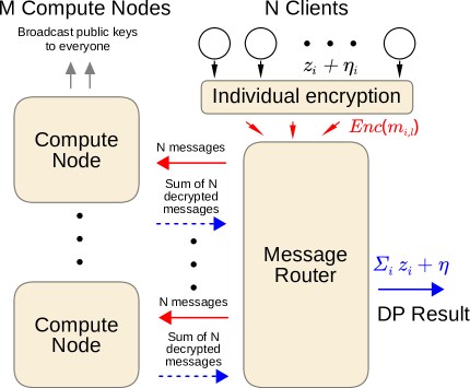
(a) DCA setting

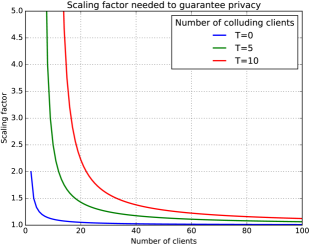
(b) Extra scaling factor

Figure 1: 1(a): Schematic diagram of the Distributed Compute algorithm (DCA). Red refers to encrypted values, blue to unencrypted (but blinded or DP) values. 1(b) Extra scaling factor needed for the noise in the distributed setting with $T$ colluding clients as compared to the trusted aggregator setting.

In order to add the correct amount of noise while avoiding revealing the unperturbed data to any single party, we combine an encryption scheme with the Gaussian mechanism for DP as illustrated in Fig. 1(a). Each individual client adds a small amount of Gaussian noise to his data, resulting in the aggregated noise to be another Gaussian with large enough variance. The details of the noise scaling are presented in the Section 4.1.2.

The scheme relies on several independent aggregators, called Compute nodes (Algorithm 1). At a general level, the clients divide their data and some blinding noise into shares that are each sent to one Compute. After receiving shares from all clients, each Compute decrypts the values, sums them and broadcasts the results. The final results can be obtained by summing up the values from all Computes, which cancels the blinding noise.

Algorithm 1 Distributed Compute Algorithm for distributed summation with independent Compute nodes

0:  Distributed Gaussian mechanism noise variances $\sigma^{2}_{j}$, $j=1,\dots,d$ (public); Number of parties $N$ (public); Number of Compute nodes $M$ (public) $d$-dimensional vectors $\mathbf{z}_{i}$ held by clients $i\in\{1,\dots,N\}$

0:  Differentially private sum $\sum_{i=1}^{N}\left(\mathbf{z}_{i}+\boldsymbol{\eta}_{i}\right)$, where $\boldsymbol{\eta}_{i}\sim\mathcal{N}(0,\mathrm{diag}(\sigma_{j}^{2}))$

1:  Each client $i$ simulates $\boldsymbol{\eta}_{i}\sim\mathcal{N}(0,\mathrm{diag}(\sigma^{2}_{j}))$ and $M-1$ vectors $\mathbf{r}_{i,k}$ of uniformly random fixed-point data with $\mathbf{r}_{i,M}=\sum_{l=1}^{M-1}$ to ensure that $\sum_{k=1}^{M}\mathbf{r}_{i,k}=\mathbf{0}_{d}$ (a vector of zeros).

2:  Each client $i$ computes the messages $\mathbf{m}_{i,1}=\mathbf{z}_{i}+\boldsymbol{\eta}_{i}+\mathbf{r}_{i,1}$, $\mathbf{m}_{i,k}=\mathbf{r}_{i,k},k=2,\dots M$, and sends them securely to the corresponding Compute $k$.

3:  After receiving messages from all of the clients, Compute $k$ decrypts the values and broadcasts the noisy aggregate sums $\mathbf{q}_{k}=\sum_{i=1}^{N}m_{i,k}$. A final aggregator will then add these to obtain $\sum_{k=1}^{M}\mathbf{q}_{k}=\sum_{i=1}^{N}(\mathbf{z}_{i}+\boldsymbol{\eta}_{i})$.

4.1.1 Threat model

We assume there are at most $T$ clients who may collude to break the privacy, either by revealing the noise they add to their data samples or by abstaining from adding the noise in the first place. The rest are honest-but-curious (HbC), i.e., they will take a peek at other people’s data if given the chance, but they will follow the protocol.

To break the privacy of individual clients, all Compute nodes need to collude. We therefore assume that at least one Compute node follows the protocol. We further assume that all parties have an interest in the results and hence will not attempt to pollute the results with invalid values.

4.1.2 Privacy of the mechanism

In order to guarantee that the sum-query results returned by Algorithm 1 are DP, we need to show that the variance of the aggregated Gaussian noise is large enough.

Theorem 1 (Distributed Gaussian mechanism).

If at most $T$ clients collude or drop out of the protocol, the sum-query result returned by Algorithm 1 is $(\epsilon,\delta)$-DP, when the variance of the added noise $\sigma_{j}^{2}$ fulfils

$$\sigma_{j}^{2}\geq\frac{1}{N-T-1}\sigma_{j,std}^{2},$$

where $N$ is the number of clients and $\sigma_{j,std}^{2}$ is the variance of the noise in the standard $(\epsilon,\delta)$-DP Gaussian mechanism given in Eq. (1).

Proof.

See Supplement. ∎

In the case of all HbC clients, $T=0$. The extra scaling factor increases the variance of the DP, but this factor quickly approaches $1$ as the number of clients increases, as can be seen from Figure 1(b).

4.1.3 Fault tolerance

The Compute nodes need to know which clients’ contributions they can safely aggregate. This feature is simple to implement e.g. with pairwise-communications between all Compute nodes. In order to avoid having to start from scratch due to insufficient noise for DP, the same strategy used to protect against colluding clients can be utilized: when $T>0$, at most $T$ clients in total can drop or collude and the scheme will still remain private.

4.1.4 Computational scalability

Most of the operations needed in Algorithm 1 are extremely fast: encryption and decryption can use fast symmetric algorithms such as AES (using slower public key cryptography just for the key of the symmetric system) and the rest is just integer additions for the fixed point arithmetic. The likely first bottlenecks in the implementation would be caused by synchronisation when gathering the messages as well as the generation of cryptographically secure random vectors $\mathbf{r}_{i,k}$.

4.2 Differentially private Bayesian learning on distributed data

In order to perform DP Bayesian learning securely in the distributed setting, we use DCA (Algorithm 1) to compute the required data summaries that correspond to Eq. (3). In this Section we consider how to combine this scheme with concrete DP learning methods introduced for the trusted aggregator setting, so as to provide a wide range of possibilities for performing DP Bayesian learning securely with distributed data.

The aggregation algorithm is most straightforward to apply to the SSP method [14, 17] for exact and approximate posterior inference on exponential family models. [14] and [17] use Laplacian noise to guarantee $\epsilon$-DP, which is a stricter form of privacy than the $(\epsilon,\delta)$-DP used in DCA [10]. We consider here only $(\epsilon,\delta)$-DP version of the methods, and discuss the possible Laplace noise mechanism further in Section 8. The model training in this case is done in a single iteration, so a single application of Algorithm 1 is enough for learning. We consider a more detailed example in Section 4.2.1.

We can apply DCA also to DP variational inference [18, 20]. These methods rely on possibly clipped gradients or expected sufficient statistics calculated from the data. Typically, each training iteration would use only a mini-batch instead of the full data. To use variational inference in the distributed setting, an arbitrary party keeps track of the current (public) model parameters and the privacy budget, and asks for updates from the clients.

At each iteration, the model trainer selects a random mini-batch of fixed public size from the available clients and sends them the current model parameters. The selected clients then calculate the clipped gradients or expected sufficient statistics using their data, add noise to the values scaled reflecting the batch size, and pass them on using DCA. The model trainer receives the decrypted DP sums from the output and updates the model parameters.

4.2.1 Distributed Bayesian Linear Regression with Data Projection

As an empirical example, we consider Bayesian linear regression (BLR) with data projection in the distributed setting. The standard BLR model depends on the data only through sufficient statistics and the approach discussed in Section 4.2 can be used in a straightforward manner to fit the model by running a single round of DCA.

The more efficient BLR with projection (Algorithm 2) [17] reduces the data range, and hence sensitivity, by non-linearly projecting all data points inside stricter bounds, which translates into less added noise. We can select the bounds to optimize bias vs. DP noise variance. In the distributed setting, we need to run an additional round of DCA and use some privacy budget to estimate data standard deviations (stds). However, as shown by the test results (Figure 2), this can still achieve significantly better utility with a given privacy level.

Algorithm 2 Distributed linear regression with projection

0:  Number of clients $N$ (public), data and target values $(x_{ij},y_{i}),j=1,\dots,d$ held by clients $i\in\{1,\dots,N\}$, assumed data and target bounds $(-c_{j},c_{j}),j=1,\dots,d+1$ (public), privacy budget $(\epsilon,\delta)$ (public),

0:  DP BLR model sufficient statistics of projected data $\sum_{i=1}^{N}\hat{\mathbf{x}}_{i}\hat{\mathbf{x}}_{i}^{T}+\boldsymbol{\eta}^{(1)}$, $\sum_{i=1}^{N}\hat{\mathbf{x}}_{i}^{T}\hat{y}_{i}+\boldsymbol{\eta}^{(2)}$, calculated using projection to estimated optimal bounds

1:  Each client projects his data to the assumed bounds $(-c_{j},c_{j})\ \forall j$.

2:  Calculate marginal std estimates $\sigma^{(1)},\dots,\sigma^{(d+1)}$ by running Algorithm 1 using the assumed bounds for sensitivity and a chosen share of the privacy budget.

3:  Estimate optimal projection thresholds $p_{j},j=1,\dots,d+1$ as fractions of std on auxiliary data. Each client then projects his data to the estimated optimal bounds $(-p_{j}\sigma^{(j)},p_{j}\sigma^{(j)}),j=1,\dots,d+1$.

4:  Aggregate the unique terms in the DP sufficient statistics by running Algorithm 1 using the estimated optimal bounds for sensitivity and the remaining privacy budget, and combine the DP result vectors into the symmetric $d\times d$ matrix and $d$-dimensional vector of DP sufficient statistics.

The assumed bounds in Step 1 of Algorithm 2 would typically be available from general knowledge of the data. The projection in Step 1 ensures the privacy of the scheme even if the bounds are invalid for some samples. We determine the optimal projection thresholds $p_{j}$ in Step 3 using the same general approach as [17]: we create an auxiliary data set of equal size as the original with data generated as

$$x_{i} \sim N(0,I_{d})$$ (4)

$$\beta \sim N(0,\lambda_{0}I)$$ (5)

$$y_{i}|x_{i} \sim N(x_{i}^{T}\beta,\lambda).$$ (6)

We then perform grid search on the auxiliary data with varying thresholds to find the optimal prediction performance. The source code for our implementation is available through GitHub and a more detailed description can be found in the Supplement.

5 Experimental Setup

We demonstrate the secure DP Bayesian learning scheme in practice by testing the performance of the BLR with data projection, the implementation of which was discussed in Section 4.2.1, along with the DCA (Algorithm 1) in the all HbC clients distributed setting ($T=0$).

With the DCA our primary interest is scalability. In the case of BLR implementation, we are mostly interested in comparing the distributed algorithm to the trusted aggregator version as well as comparing the performance of the straightforward BLR to the variant using data projection, since it is not clear a priori if the extra cost in privacy necessitated by the projection in the distributed setting is offset by the reduced noise level.

We use simulated data for the DCA scalability testing, and real data for the BLR tests. As real data, we use the Wine Quality [6] (split into white and red wines) and Abalone data sets from the UCI repository[19], as well as the Genomics of Drug Sensitivity in Cancer (GDSC) project data . The measured task in the GDSC data is to predict drug sensitivity of cancer cell lines from gene expression data (see Supplement for a more detailed description). The datasets are assumed to be zero-centred. This assumption is not crucial but is done here for simplicity; non-zero data means can be estimated like the marginal stds at the cost of some added noise (see Section 4.2.1).

For estimating the marginal std, we also need to assume bounds for the data. For unbounded data, we can enforce arbitrary bounds simply by projecting all data inside the chosen bounds, although very poor choice of bounds will lead to poor performance. With real distributed data, the assumed bounds could differ from the actual data range. In the UCI tests we simulate this effect by scaling each data dimension to have a range of length $10$, and then assuming bounds of $[-7.5,7.5]$, i.e., the assumed bounds clearly overestimate the length of the true range, thus adding more noise to the results. The actual scaling chosen here is arbitrary. With the GDSC data, the true range is known due to the nature of the data (see Supplement).

The optimal projection thresholds are searched for using 10 repeats on a grid with $20$ points between $0.1$ and $2.1$ times the std of the auxiliary data set. In the search we use one common threshold for all data dimensions and a separate one for the target.

For accuracy measure, we use prediction accuracy on a separate test data set. The size of the test set for UCI in Figure 2 is $500$ for red wine, 1000 for white wine, and 1000 for abalone data. The test set size for GDSC in Figure 3 is 100. For UCI, we compare the median performance measured on mean absolute error over 25 cross-validation (CV) runs, while for GDSC we measure mean prediction accuracy to sensitive vs insensitive with Spearman’s rank correlation on 30 CV runs. In both cases, we use input perturbation [12] and the trusted aggregator setting as baselines.

6 Results

	N=$10^{2}$	N=$10^{3}$	N=$10^{4}$	N=$10^{5}$
d=10	1.72	1.89	2.99	8.58
d=$10^{2}$	2.03	2.86	12.36	65.64
d=$10^{3}$	3.43	10.56	101.2	610.55
d=$10^{4}$	15.30	84.95	994.96	1592.29

Table 1: DCA experiment average runtimes in seconds with 5 repeats, using M=10 Compute nodes, N clients and vector length d.

Table 1 shows runtimes of a distributed Spark implementation of the DCA algorithm. The timing excludes encryption, but running AES for the data of the largest example would take less than 20 s on a single thread on a modern CPU. The runtime modestly increases as $N$ or $d$ is increased. This suggests that the prototype is reasonably scalable. Spark overhead sets a lower bound runtime of approximately 1 s for small problems. For large $N$ and $d$, sequential communication at the 10 Compute threads is the main bottleneck. Larger $N$ could be handled by introducing more Compute nodes and clients only communicating with a subset of them.

Comparing the results on predictive error with and without projection (Fig. 2 and Fig. 3), it is clear that despite incurring extra privacy cost for having to estimate the marginal standard deviations, using the projection can improve the results markedly with a given privacy budget.

The results also demonstrate that compared to the trusted aggregator setting, the extra noise added due to the distributed setting with HbC clients is insignificant in practice as the results of the distributed and trusted aggregator algorithms are effectively indistinguishable.

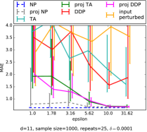
(a) Red wine data set

(b) Abalone data set

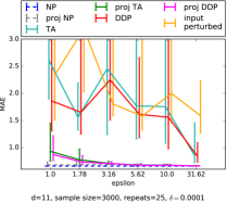
(c) White wine data set

Figure 2: Median of the predictive accuracy measured on mean absolute error (MAE) on several UCI data sets with error bars denoting the interquartile range (lower is better). The performance of the distributed methods (DDP, DDP proj) is indistinguishable from the corresponding undistributed algorithms (TA, TA proj) and the projection (proj TA, proj DDP) can clearly be beneficial for prediction performance. NP refers to non-private version, TA to the trusted aggregator setting, DDP to the distributed scheme.

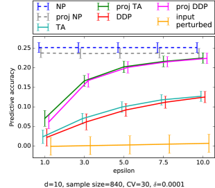
(a) Drug sensitivity prediction

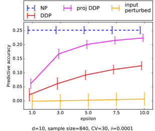
(b) Drug sensitivity prediction, selected methods

Figure 3: Mean drug sensitivity prediction accuracy on GDSC dataset with error bars denoting standard deviation over CV runs (higher is better). Distributed results (DDP, proj DDP) do not differ markedly from the corresponding trusted aggregator (TA, proj TA) results. The projection (proj TA, proj DDP) is clearly beneficial for performance. The actual sample size varies between drugs. NP refers to non-private version, TA to the trusted aggregator setting, DDP to the distributed scheme.

7 Related Work

The idea of distributed private computation through addition of noise generated in a distributed manner was first proposed by Dwork et al. [11]. However, to the best of our knowledge, there is no prior work on secure DP Bayesian statistical inference in the distributed setting.

In machine learning, [21] presented the first method for aggregating classifiers in a DP manner, but their approach is sensitive to the number of parties and sizes of the data sets held by each party and cannot be applied in a completely distributed setting. [22] improved upon this by an algorithm for distributed DP stochastic gradient descent that works for any number of parties. The privacy of the algorithm is based on perturbation of gradients which cannot be directly applied to the efficient SSP mechanism. The idea of aggregating classifiers was further refined in [16] through a method that uses an auxiliary public data set to improve the performance.

The first practical method for implementing DP queries in a distributed manner was the distributed Laplace mechanism presented in [23]. The distributed Laplace mechanism could be used instead of the Gaussian mechanism if pure $\epsilon$-DP is required, but the method, like those in [21, 22], needs homomorphic encryption which can be computationally more demanding for high-dimensional data.

There is a wealth of literature on secure distributed computation of DP sum queries as reviewed in [15]. The methods of [24, 2, 3, 15] also include different forms of noise scaling to provide collusion resistance and/or fault tolerance, where the latter requires a separate recovery round after data holder failures which is not needed by DCA. [13] discusses low level details of an efficient implementation of the distributed Laplace mechanism.

Finally, [28] presents several proofs related to the SMC setting and introduce a protocol for generating approximately Gaussian noise in a distributed manner. Compared to their protocol, our method of noise addition is considerably simpler and faster, and produces exactly instead of approximately Gaussian noise with negligible increase in noise level.

8 Discussion

We have presented a general framework for performing DP Bayesian learning securely in a distributed setting. Our method combines a practical SMC method for calculating secure sum queries with efficient Bayesian DP learning techniques adapted to the distributed setting.

DP methods are based on adding sufficient noise to effectively mask the contribution of any single sample. The extra loss in accuracy due to DP tends to diminish as the number of samples increases and efficient DP estimation methods converge to their non-private counterparts as the number of samples increases [14, 17]. A distributed DP learning method can significantly help in increasing the number of samples because data held by several parties can be combined thus helping make DP learning significantly more effective.

Considering the DP and the SMC components separately, although both are necessary for efficient learning, it is clear that the choice of method to use for each sub-problem can be made largely independently. Assessing these separately, we can therefore easily change the privacy mechanism from the Gaussian used in Algorithm 1 to the Laplace mechanism, e.g. by utilising one of the distributed Laplace noise addition methods presented in [15] to obtain a pure $\epsilon$-DP method. If need be, the secure sum algorithm in our method can also be easily replaced with one that better suits the security requirements at hand.

While the noise introduced for DP will not improve the performance of an otherwise good learning algorithm, a DP solution to a learning problem can yield better results if the DP guarantees allow access to more data than is available without privacy. Our distributed method can further help make this more efficient by securely and privately combining data from multiple parties.

Acknowledgements

This work was funded by the Academy of Finland [303815 to S.T., 303816 to S.K. , Centre of Excellence COIN, 283193 to S.K., 294238 to S.K., 292334 to S.K., 278300 to A.H., 259440 to A.H. and 283107 to A.H.] and the Japan Agency for Medical Research and Development (AMED).

Supplement

This supplement contains proofs and extra discussion omitted from the main text.

9 Privacy and fault tolerance

Theorem 2 (Distributed Gaussian mechanism).

If at most $T$ clients collude or drop out of the protocol, the sum-query result returned by Algorithm 1 is differentially private, when the variance of the added noise $\sigma_{j}^{2}$ fulfils

$$\sigma_{j}^{2}\geq\frac{1}{N-T-1}\sigma_{j,std}^{2},$$

where $N$ is the number of clients and $\sigma_{j,std}^{2}$ is the variance of the noise in the standard Gaussian mechanism given in Eq. (1).

Proof.

Using the property that a sum of independent Gaussian variables is another Gaussian with variance equal to the sum of the component variances, we can divide the total noise equally among the $N$ clients.

However, in the distributed setting even with all honest-but-curious clients, there is an extra scaling factor needed compared to the standard DP. Since each client knows the noise values she adds to the data, she can also remove them from the aggregate values. In other words, privacy then has to be guaranteed by the noise the remaining $N-1$ clients add to the data. If we further assume the possibility of $T$ colluding clients, then the noise from $N-T-1$ clients must be sufficient to guarantee the privacy.

The added noise can therefore be calculated from the inequality

$$\sum_{i=1}^{N-T-1}\sigma_{j}^{2}\geq \sigma_{j,std}^{2}$$ (7)

$$\Leftrightarrow\ \sigma_{j}^{2}\geq \frac{1}{N-T-1}\sigma_{j,std}^{2}.$$ (8)

∎

10 Bayesian linear regression

In the following, we denote the $i$th observation in $d$-dimensional data by $\mathbb{x}_{i}$, the scalar target values by $y_{i}$, and the whole $d+1-$dimensional dataset by $D_{i}=(\mathbb{x}_{i},y_{i})$. We assume all column-wise expectations to be zeroes for simplicity. For $n$ observations, we denote the sufficient statistics by $n\bar{xx}=\sum_{i=1}^{n}\mathbb{x}_{i}\mathbb{x}_{i}^{T}$ and $n\bar{xy}=\sum_{i=1}^{n}\mathbb{x}_{i}y_{i}$.

For the regression, we assume that

$$y_{i}|\mathbb{x}_{i}\sim N(\mathbb{x}_{i}^{T}\mathbb{\beta},\lambda I),i=1,\dots,n$$ (9)

$$\mathbb{\beta}\sim N(0,\lambda_{0}I),$$ (10)

where we want to learn the posterior over $\beta$, and $\lambda,\lambda_{0}$ are hyperparameters (set to $1$ in the tests). The posterior can be solved analytically to give

$$\beta|\mathbb{y},\mathbb{x} \sim N(\hat{\mu},\hat{\Lambda}),$$ (11)

$$\hat{\Lambda} =\lambda_{0}I+\lambda n\bar{xx},$$ (12)

$$\hat{\mu} =\hat{\Lambda}^{-1}(\lambda n\bar{xy}).$$ (13)

The predicted values from the model are $\hat{y}=\mathbb{x}^{T}\hat{\mu}$.

The DP sufficient statistics are given by $n\hat{xx}=n\bar{xx}+\eta_{xx},n\hat{xy}=n\bar{xy}+\eta_{xy}$, where $\eta_{xx},\eta_{xy}$ consist of suitably scaled Gaussian noise added independently to each dimension. In total, there are $d(d+1)/2+d$ parameters in the combined sufficient statistic, since $n\bar{xx}$ is a symmetric matrix.

The main idea in the data projection is simply to project the data into some reduced range. Since the noise level is determined by the sensitivity of the data, reducing the sensitivity by limiting the data range translates into less added noise.

With projection threshold $c$, the projection of data $x_{i}$ is given by

$$\breve{x_{i}}=\max(-c,\min(x_{i},c)).$$ (14)

This data projection obviously discards information, but in various problems it can be beneficial to disregard some information in the data in order to achieve less noisy estimates of the model parameters. From the bias-variance trade-off point of view, this can be seen as increasing the bias while reducing the variance. The optimal trade-off then depends on the actual problem.

To run Algorithm 2 (in the main text), we need to assume projection bounds $(c_{j},d_{j})$ for each dimension $j\in\{1,\dots,d+1\}$ for the data $(\mathbb{x}_{i},y_{i})_{i=1}^{n}$. In the paper we assume bounds of the form $(-c_{j},c_{j})$. To find good projection bounds, we first find an optimal projection threshold by a grid search on an auxiliary dataset, that is generated from a BLR model similar to the regression model defined above.

This gives us the projection thresholds in terms of std for each dimension. We then estimate the marginal std for each dimension by using Algorithm 1 (in the main text), to fix the actual projection thresholds. For this the data is assumed to lie on some known bounded interval. In practice, the assumed bounds need to be based on prior information. In case the estimates are negative due to noise, they are set to small positive constants ($0.5$ in all the tests).

The amount of noise each client needs to add to the output depends partly on the sensitivity of the function in question. The query function we are interested in returns a vector of length $d(d+1)/2+d$ that contains all the unique terms in the sufficient statistics needed for linear regression.

Let $\mathbb{x},\mathbb{y}$ be the mismatching, maximally different elements over adjacent datasets s.t. dimensions $1,\dots,d$ are the independent variables, and $d+1$ is the target. Assume further that each dimension $j=1,\dots,d+1$ is bounded by $(-c_{j},c_{j})$. The squared sensitivity of the query $f$ is then

$$\Delta_{2}(f)^{2} =||f(\mathbb{x})-f(\mathbb{y})||_{2}^{2}$$ (15)

$$=||(x_{j}x_{k}-y_{j}y_{k},x_{j}x_{d+1}-y_{j}y_{d+1})_{j=1,k=j}^{d}||_{2}^{2}$$ (16)

$$=\sum_{j=1}^{d}\sum_{k=j}^{d}(x_{j}x_{k}-y_{j}y_{k})^{2}+\sum_{j=1}^{d}(x_{j}x_{d+1}-y_{j}y_{d+1})^{2}$$ (17)

$$\leq\sum_{j=1}^{d}(c_{j}^{2})^{2}+\sum_{j=1}^{d}\sum_{k>j}^{d}(2c_{j}c_{k})^{2}+\sum_{j=1}^{d}(2c_{j}c_{d+1})^{2}.$$ (18)

We assume $c_{j}=c_{x}\forall j=1,\dots,d$, so (18) can be further simplified to $d(2d-1)c_{x}^{4}+4d(c_{x}c_{d+1})^{2}$.

11 GDSC dataset description

The data were downloaded from the Genomics of Drug Sensitivity in Cancer (GDSC) project, release 6.1, March 2017, http://www.cancerrxgene.org/. We use gene expression and drug sensitivity data. The gene expression dimensionality is reduced to 10 genes used for the actual prediction task, based on prior information about their mutation counts in cancer (we use the same procedure as [17]). The dataset used for learning contains 940 cell lines and drug sensitivity data for 265 drugs. Some of the values are missing, so the actual number of observations varies between the drugs. We use a test set of size 100 and the rest of the available data for learning.

Since we want to focus on the relative expression of the genes, each data point is normalized to have $l_{2}$-norm of 1. In the distributed setting this can be done by each client without breaching privacy. After the scaling, we also know that the sensitivity of each dimension is at most 1. For the target value, we assume a range of [-7.5,7.5] for the marginal standard deviation estimation. The true range varies between drugs, with the length of all the ranges less than 12. In other words, the estimate used adds some amount of extra noise to the results.

12 Asymptotic efficiency of the Gaussian mechanism

The asymptotic efficiency of the sufficient statistics perturbation using Laplace mechanism has been proven before [14, 17]. We show corresponding results for the Gaussian mechanism. The proofs generally follow closely those given in [17]. For convenience, we state the relevant definitions, but mostly focus on those proofs that differ in a non-trivial way from the existing ones for the Laplace mechanism. For the full proofs and related discussion, see [17].

12.1 Definition of asymptotic efficiency

Definition 12.1.

A differentially private mechanism $\mathcal{M}$ is asymptotically consistent with respect to an estimated parameter $\theta$ if the private estimates $\hat{\theta}_{\mathcal{M}}$ given a data set $\mathcal{D}$ converge in probability to the corresponding non-private estimates $\hat{\theta}_{NP}$ as the number of samples, $n=|\mathcal{D}|$, grows without bound, i.e., if for any $\alpha>0$,

$$\lim\limits_{n\rightarrow\infty}\mathrm{Pr}\{\|\hat{\theta}_{\mathcal{M}}-\hat{\theta}_{NP}\|>\alpha\}=0.$$

Definition 12.2.

A differentially private mechanism $\mathcal{M}$ is asymptotically efficiently private with respect to an estimated parameter $\theta$, if the mechanism is asymptotically consistent and the private estimates $\hat{\theta}_{\mathcal{M}}$ converge to the corresponding non-private estimates $\hat{\theta}_{NP}$ at the rate $\mathcal{O}(1/n)$, i.e., if for any $\alpha>0$ there exist constants $C,N$ such that

$$\mathrm{Pr}\{\|\hat{\theta}_{\mathcal{M}}-\hat{\theta}_{NP}\|>C/n\}<\alpha$$

for all $n\geq N$.

The first part of Theorem 3 follows closely the corresponding result for the Laplace mechanism [17, Theorem 1]. The theorem shows that the optimal rate for estimating the expectation of exponential family distributions is $\mathcal{O}(1/n)$. This justifies the term asymptotically efficiently private introduced by [17], when we show that sufficient statistics perturbation by the Gaussian mechanism achieves this rate.

Theorem 3.

The private estimates $\hat{\theta}_{\mathcal{M}}$ of an exponential family posterior expectation parameter $\theta$, generated by a differentially private mechanism $\mathcal{M}$ that achieves $(\epsilon,\delta)$-differential privacy for any $\epsilon>0,\delta\in(0,1)$, cannot converge to the corresponding non-private estimates $\hat{\theta}_{NP}$ at a rate faster than $1/n$. That is, assuming $\mathcal{M}$ is $(\epsilon,\delta)$-differentially private, there exists no function $f(n)$ such that $\lim\sup nf(n)=0$ and for all $\alpha>0$, there exists a constant $N$ such that

$$\mathrm{Pr}\{\|\hat{\theta}_{\mathcal{M}}-\hat{\theta}_{NP}\|>f(n)\}<\alpha$$

for all $n\geq N$.

Proof.

The non-private estimate of an expectation parameter of an exponential family is [7]

$$\hat{\theta}_{NP}|x_{1},\dots,x_{n}=\frac{n_{0}x_{0}+\sum_{i=1}^{n}x_{i}}{n_{0}+n}.$$ (19)

The difference of the estimates from two neighbouring data sets differing by one element is

$$(\hat{\theta}_{NP}|\mathcal{D})-(\hat{\theta}_{NP}|\mathcal{D}^{\prime})=\frac{x-y}{n_{0}+n},$$ (20)

where $x$ and $y$ are the corresponding mismatched elements. Let $\Delta=\max(\|x-y\|)$, and let $\mathcal{D}$ and $\mathcal{D}^{\prime}$ be neighbouring data sets including these maximally different elements.

Let us assume that there exists a function $f(n)$ such that $\lim\sup nf(n)=0$ and for all $\alpha>0$ there exists a constant $N$ such that

$$\mathrm{Pr}\{\|\hat{\theta}_{\mathcal{M}}-\hat{\theta}_{NP}\|>f(n)\}<\alpha$$

for all $n\geq N$.

Fix $\alpha>0$ and choose $M\geq\max(N,n_{0})$ such that

$$f(n)\leq\Delta/4n$$

for all $n\geq M$. This implies that

$$\|(\hat{\theta}_{NP}|\mathcal{D})-(\hat{\theta}_{NP}|\mathcal{D}^{\prime})\|=\frac{\Delta}{n_{0}+n}\geq\frac{\Delta}{2n}\geq 2f(n).$$ (21)

Let us define the region

$$C_{\mathcal{D}}=\{t\;|\;\|(\hat{\theta}_{NP}|\mathcal{D})-t\|<f(n)\}.$$

Based on our assumptions we have

$$\mathrm{Pr}(\hat{\theta}_{\mathcal{M}}|\mathcal{D}\in C_{\mathcal{D}})> 1-\alpha$$ (22)

$$\mathrm{Pr}(\hat{\theta}_{\mathcal{M}}|\mathcal{D}^{\prime}\in C_{\mathcal{D}})< \alpha$$ (23)

$$\mathrm{Pr}(\hat{\theta}_{\mathcal{M}}|\mathcal{D}\in C_{\mathcal{D}})\leq \exp(\epsilon)\mathrm{Pr}(\hat{\theta}_{\mathcal{M}}|\mathcal{D}^{\prime}\in C_{\mathcal{D}})+\delta$$ (24)

which implies that

$$1-\alpha< \exp(\epsilon)\alpha+\delta$$ (25)

$$\Leftrightarrow\ \delta> 1-(1+\exp(\epsilon))\alpha.$$ (26)

Since for fixed $\epsilon$, $\lim_{\alpha\rightarrow 0}1-(1+\exp(\epsilon))\alpha=1$, $\mathcal{M}$ cannot be $(\epsilon,\delta)$-differentially private with any $\epsilon$ and $\delta<1$. ∎

Before the next theorem, we prove Lemma 1, which is not used in [17].

Lemma 1.

Let $x\in\mathbb{R}^{d}$, $x\sim N(0,\sigma^{2}I)$. The tail probability of the $\ell_{1}$ norm of $x$ obeys

$$\mathrm{Pr}(\|x\|_{1}\geq t)\leq\frac{d\sigma^{2}}{\left(t-\sqrt{2/\pi}d\sigma\right)^{2}}\left(1-\frac{2}{\pi}\right).$$ (27)

Proof.

$\|x\|_{1}=\sum_{i=1}^{d}|x_{i}|=\sum_{i=1}^{d}y_{i}$, where $x_{i}\sim N(0,\sigma^{2})$ and $y_{i}$ follows the half-normal distribution with variance $\sigma^{2}$.

It is known that $\operatorname{E}[y_{i}]=\sqrt{2/\pi}\sigma$ and $\operatorname{Var}[y_{i}]=\sigma^{2}(1-2/\pi)$.

Because $y_{i}$ are independent, $\operatorname{E}[\|x\|_{1}]=d\operatorname{E}[y_{i}]=\sqrt{2/\pi}d\sigma$ and $\operatorname{Var}[\|x\|_{1}]=d\operatorname{Var}[y_{i}]=d\sigma^{2}(1-2/\pi)$.

Setting $a=t-\sqrt{2/\pi}d\sigma$ we have

$$\mathrm{Pr}(\|x\|_{1}\geq t) =\mathrm{Pr}\left(\|x\|_{1}\geq a+\sqrt{2/\pi}d\sigma\right)$$

$$\leq\mathrm{Pr}\left(\left|\|x\|_{1}-\sqrt{2/\pi}d\sigma\right|\geq a\right)$$

$$\leq\frac{d\sigma^{2}}{\left(t-\sqrt{2/\pi}d\sigma\right)^{2}}\left(1-\frac{2}{\pi}\right).$$

where the last inequality follows from Chebyshev’s inequality. ∎

12.1.1 Asymptotic efficiency of Gaussian means

Theorem 4, showing one case of asymptotic efficiency of the Gaussian mechanism, corresponds to [17, Theorem 5], although the proof is somewhat different.

Theorem 4.

$(\epsilon,\delta)$-differentially private estimate of the mean of a $d$-dimensional Gaussian variable $x$ bounded by $\|x_{i}\|_{1}\leq B$ in which the Gaussian mechanism is used to perturb the sufficient statistics, is asymptotically efficiently private.

Proof.

Following [17, Theorem 3], it is trivial to show that

$$\|\mu_{DP}-\mu_{NP}\|_{1}\leq\frac{c}{n}\|\delta\|_{1},$$

where $\delta=(\delta_{1},\dots,\delta_{d})^{T}\in\mathbb{R}^{D}$ with $\delta_{j}\sim\mathrm{N}\left(0,\sigma_{j}^{2}\right)$ holds when we utilize the Gaussian mechanism instead of the Laplace mechanism. This allows us to bound the corresponding tail probabilities by using Lemma 1.

Therefore, given $\alpha>0$, we can guarantee that

$$\mathrm{Pr}\left\{\|\mu_{DP}-\mu_{NP}\|_{1}>\frac{C}{n}\right\}\leq \mathrm{Pr}\left\{\frac{1}{n}\|\delta\|_{1}>\frac{C}{n}\right\}$$ (28)

$$= \mathrm{Pr}\{\|\delta\|_{1}>C\}<\alpha,$$ (29)

by choosing $C$ according to Lemma 1. ∎

12.2 Asymptotic efficiency of DP linear regression

Theorem 5 that establishes asymptotic efficiency for DP linear regression using the Gaussian mechanism, for the most part follows [17, Theorem 8]. We concentrate here more closely only on the differing parts.

Theorem 5.

$(\epsilon,\delta)$-differentially private inference of the posterior mean of the weights of linear regression with the Gaussian mechanism used to perturb the sufficient statistics is asymptotically efficiently private.

Proof.

Following the proof of [17, Theorem 7] with minimal changes we have

$$\left\|\mu_{DP}-\mu_{NP}\right\|_{1}\leq\left\|(\Lambda_{0}+\Lambda(n\bar{xx}+\Delta))^{-1}\Lambda\delta\right\|_{1}\\ +\Bigg{\|}\left[\left(\frac{1}{n}\Lambda_{0}+\Lambda\left(\bar{xx}+\frac{1}{n}\Delta\right)\right)^{-1}-\left(\frac{1}{n}\Lambda_{0}+\Lambda\bar{xx}\right)^{-1}\right]\\ \times\left(\Lambda\bar{xy}+\frac{1}{n}\Lambda_{0}\beta_{0}\right)\Bigg{\|}_{1}$$ (30)

where $\Delta$ is the noise contribution from the Gaussian mechanism added to the sufficient statistics $\bar{xx}$ (see Section 10 in this supplement).

As in [17, Theorem 7], the first term can be bounded as

$$\left\|(\Lambda_{0}+\Lambda(n\bar{xx}+\Delta))^{-1}\Lambda\delta\right\|_{1} \leq\frac{c_{1}}{n}\left\|(\bar{xx})^{-1}\right\|_{1}\|\delta\|_{1}$$ (31)

where $c_{1}>1$, for large enough $n$.

As done in the proof of Theorem 4, given $\alpha>0$, Lemma 1 can be used to ensure that

$$\mathrm{Pr}\left\{\|(\Lambda_{0}+\Lambda(n\bar{xx}+\Delta))^{-1}\Lambda\delta\|_{1}>\frac{C_{1}}{n}\right\}<\frac{\alpha}{2},$$ (32)

by choosing a suitable $C_{1}$.

Again, following [17, Theorem 7], the second term can be bounded as

$$\Bigg{\|}\left[\left(\frac{1}{n}\Lambda_{0}+\Lambda\left(\bar{xx}+\frac{1}{n}\Delta\right)\right)^{-1}-\left(\frac{1}{n}\Lambda_{0}+\Lambda\bar{xx}\right)^{-1}\right]\\ \times\left(\Lambda\bar{xy}+\frac{1}{n}\Lambda_{0}\beta_{0}\right)\Bigg{\|}_{1}\\ \leq\frac{c_{2}}{n}\left\|\left(\bar{xx}\right)^{-1}\right\|_{1}\left\|\Delta\right\|_{1}\left\|\left(\bar{xx}\right)^{-1}\right\|_{1}\left\|\bar{xy}\right\|_{1},$$

where, as in Eq. (31), the bound is valid for $c_{2}>1$ as $n$ gets large enough.

$\|\Delta\|_{1}$ here is the $l_{1}$-norm of the symmetric matrix $\Delta$, that is comprised of a vector of $d(d+1)/2$ unique noise terms, each generated independently from a Normal distribution according to the Gaussian mechanism. Denoting this vector by $\mathbb{v}$, a bound to the matrix norm is given by $\|\Delta\|_{1}\leq\|\mathbb{v}\|_{1}$.

Therefore, given $\alpha>0$, we can again use Lemma 1 to find a suitable $C_{2}$ s.t.

$$\mathrm{Pr}\left\{\left\|\Delta\right\|_{1}>\frac{C_{2}}{c_{2}\left\|\left(\bar{xx}\right)^{-1}\right\|_{1}^{2}\left\|\bar{xy}\right\|_{1}}\right\}\\ \leq\mathrm{Pr}\left\{\left\|\mathbb{v}\right\|_{1}>\frac{C_{2}}{c_{2}\left\|\left(\bar{xx}\right)^{-1}\right\|_{1}^{2}\left\|\bar{xy}\right\|_{1}}\right\}<\frac{\alpha}{2}.$$ (33)

By combining Eqs. (32) and (33) we get

$$\mathrm{Pr}\left\{\left\|\mu_{DP}-\mu_{NP}\right\|_{1}>\frac{C_{1}+C_{2}}{n}\right\}<\alpha.$$ (34)

∎

References

- Abadi et al. [2016] M. Abadi, A. Chu, I. Goodfellow, H. B. McMahan, I. Mironov, K. Talwar, and L. Zhang. Deep learning with differential privacy. In Proc. CCS 2016, 2016. doi: 10.1145/2976749.2978318. arXiv:1607.00133 [stat.ML].
- Ács and Castelluccia [2011] G. Ács and C. Castelluccia. I have a DREAM! (DiffeRentially privatE smArt Metering). In T. Filler, T. Pevný, S. Craver, and A. Ker, editors, Information Hiding: 13th International Conference, IH 2011, Prague, Czech Republic, May 18-20, 2011, Revised Selected Papers, pages 118–132. Springer Berlin Heidelberg, Berlin, Heidelberg, 2011. ISBN 978-3-642-24178-9. doi: 10.1007/978-3-642-24178-9˙9. URL http://dx.doi.org/10.1007/978-3-642-24178-9_9.
- Chan et al. [2012] T. H. H. Chan, E. Shi, and D. Song. Privacy-preserving stream aggregation with fault tolerance. In A. D. Keromytis, editor, Financial Cryptography and Data Security: 16th International Conference, FC 2012, Kralendijk, Bonaire, Februrary 27-March 2, 2012, Revised Selected Papers, pages 200–214. Springer Berlin Heidelberg, Berlin, Heidelberg, 2012. ISBN 978-3-642-32946-3. doi: 10.1007/978-3-642-32946-3˙15. URL http://dx.doi.org/10.1007/978-3-642-32946-3_15.
- Chaudhuri and Monteleoni [2009] K. Chaudhuri and C. Monteleoni. Privacy-preserving logistic regression. In D. Koller, D. Schuurmans, Y. Bengio, and L. Bottou, editors, Advances in Neural Information Processing Systems 21, pages 289–296. Curran Associates, Inc., 2009. URL http://papers.nips.cc/paper/3486-privacy-preserving-logistic-regression.pdf.
- Chaudhuri et al. [2011] K. Chaudhuri, C. Monteleoni, and A. D. Sarwate. Differentially private empirical risk minimization. J. Mach. Learn. Res., 12:1069–1109, July 2011. ISSN 1532-4435. URL http://dl.acm.org/citation.cfm?id=1953048.2021036.
- Cortez et al. [2009] P. Cortez, A. Cerdeira, F. Almeida, T. Matos, and J. Reis. Modeling wine preferences by data mining from physicochemical properties. Decision Support Systems, 47(4):547–553, 2009. doi: 10.1016/j.dss.2009.05.016.
- Diaconis and Ylvisaker [1979] P. Diaconis and D. Ylvisaker. Conjugate priors for exponential families. Ann. Stat., 7(2):269–281, Mar 1979. ISSN 0090-5364. doi: 10.1214/aos/1176344611. URL http://dx.doi.org/10.1214/aos/1176344611.
- Dimitrakakis et al. [2013] C. Dimitrakakis, B. Nelson, Z. Zhang, A. Mitrokotsa, and B. Rubinstein. Bayesian differential privacy through posterior sampling. 2013. arXiv 1306.1066 [stat.ML], updated 2016.
- Dimitrakakis et al. [2014] C. Dimitrakakis, B. Nelson, A. Mitrokotsa, and B. I. P. Rubinstein. Robust and private Bayesian inference. In ALT 2014, volume 8776 of Lecture Notes in Computer Science, pages 291–305. Springer Science + Business Media, 2014.
- Dwork and Roth [2014] C. Dwork and A. Roth. The algorithmic foundations of differential privacy. Foundations and Trends in Theoretical Computer Science, 9(3-4):211–407, 2014. ISSN 1551-305X. doi: 10.1561/0400000042. URL http://dx.doi.org/10.1561/0400000042.
- Dwork et al. [2006a] C. Dwork, K. Kenthapadi, F. McSherry, I. Mironov, and M. Naor. Our data, ourselves: Privacy via distributed noise generation. In Advances in Cryptology (EUROCRYPT 2006), volume 4004, page 486–503. Springer Verlag, 2006a. URL https://www.microsoft.com/en-us/research/publication/our-data-ourselves-privacy-via-distributed-noise-generation/.
- Dwork et al. [2006b] C. Dwork, F. McSherry, K. Nissim, and A. Smith. Calibrating noise to sensitivity in private data analysis. In S. Halevi and T. Rabin, editors, Theory of Cryptography: Third Theory of Cryptography Conference, TCC 2006, New York, NY, USA, March 4-7, 2006. Proceedings, pages 265–284. Springer Berlin Heidelberg, Berlin, Heidelberg, 2006b. ISBN 978-3-540-32732-5. doi: 10.1007/11681878˙14. URL http://dx.doi.org/10.1007/11681878_14.
- Eigner et al. [2014] F. Eigner, A. Kate, M. Maffei, F. Pampaloni, and I. Pryvalov. Differentially private data aggregation with optimal utility. In Proceedings of the 30th Annual Computer Security Applications Conference, pages 316–325. ACM, 2014.
- Foulds et al. [2016] J. Foulds, J. Geumlek, M. Welling, and K. Chaudhuri. On the theory and practice of privacy-preserving Bayesian data analysis. In Proceedings of the Thirty-Second Conference on Uncertainty in Artificial Intelligence, UAI’16, pages 192–201, Arlington, Virginia, United States, Mar. 2016. AUAI Press. ISBN 978-0-9966431-1-5. URL http://dl.acm.org/citation.cfm?id=3020948.3020969. arXiv:1603.07294 [cs.LG].
- Goryczka and Xiong [2015] S. Goryczka and L. Xiong. A comprehensive comparison of multiparty secure additions with differential privacy. IEEE Transactions on Dependable and Secure Computing, 2015. doi: 10.1109/TDSC.2015.2484326.
- Hamm et al. [2016] J. Hamm, P. Cao, and M. Belkin. Learning privately from multiparty data. In ICML, 2016.
- Honkela et al. [2016] A. Honkela, M. Das, O. Dikmen, and S. Kaski. Efficient differentially private learning improves drug sensitivity prediction. arXiv:1606.02109, 2016.
- Jälkö et al. [2016] J. Jälkö, O. Dikmen, and A. Honkela. Differentially private variational inference for non-conjugate models. arXiv:1610.08749, 2016.
- Lichman [2013] M. Lichman. UCI machine learning repository, 2013. URL http://archive.ics.uci.edu/ml.
- Park et al. [2016] M. Park, J. Foulds, K. Chaudhuri, and M. Welling. Variational Bayes in private settings (VIPS). arXiv:1611.00340, 2016.
- Pathak et al. [2010] M. A. Pathak, S. Rane, and B. Raj. Multiparty differential privacy via aggregation of locally trained classifiers. In Proceedings of the 23rd International Conference on Neural Information Processing Systems, NIPS’10, pages 1876–1884, USA, 2010. Curran Associates Inc. URL http://dl.acm.org/citation.cfm?id=2997046.2997105.
- Rajkumar and Agarwal [2012] A. Rajkumar and S. Agarwal. A differentially private stochastic gradient descent algorithm for multiparty classification. In AISTATS, pages 933–941, 2012.
- Rastogi and Nath [2010] V. Rastogi and S. Nath. Differentially private aggregation of distributed time-series with transformation and encryption. In Proceedings of the 2010 ACM SIGMOD International Conference on Management of Data, SIGMOD ’10, pages 735–746, New York, NY, USA, 2010. ACM. ISBN 978-1-4503-0032-2. doi: 10.1145/1807167.1807247. URL http://doi.acm.org/10.1145/1807167.1807247.
- Shi et al. [2011] E. Shi, T. Chan, E. Rieffel, R. Chow, and D. Song. Privacy-preserving aggregation of time-series data. Proceedings of NDSS, 2011.
- Smith [2008] A. Smith. Efficient, differentially private point estimators. Sept. 2008. arXiv:0809.4794 [cs.CR].
- Wang et al. [2015] Y. Wang, S. E. Fienberg, and A. J. Smola. Privacy for free: Posterior sampling and stochastic gradient Monte Carlo. In Proc. ICML 2015, pages 2493–2502, 2015. URL http://jmlr.org/proceedings/papers/v37/wangg15.html.
- Williams and McSherry [2010] O. Williams and F. McSherry. Probabilistic inference and differential privacy. In Adv. Neural Inf. Process. Syst. 23, 2010.
- Wu et al. [2016] G. Wu, Y. He, J. Wu, and X. Xia. Inherit differential privacy in distributed setting: Multiparty randomized function computation. In 2016 IEEE Trustcom/BigDataSE/ISPA, pages 921–928, Aug 2016. doi: 10.1109/TrustCom.2016.0157. arXiv:1604.03001 [cs.CR].
- Zhang et al. [2012] J. Zhang, Z. Zhang, X. Xiao, Y. Yang, and M. Winslett. Functional mechanism: Regression analysis under differential privacy. PVLDB, 5(11):1364–1375, 2012. URL http://vldb.org/pvldb/vol5/p1364_junzhang_vldb2012.pdf.
- Zhang et al. [2016] Z. Zhang, B. Rubinstein, and C. Dimitrakakis. On the differential privacy of Bayesian inference. In Proc. AAAI 2016, 2016. arXiv:1512.06992 [cs.AI].