Numerical Relativity Injection Infrastructure

Abstract

This document describes the new Numerical Relativity (NR) injection infrastructure in the LIGO Algorithms Library (LAL), which henceforth allows for the usage of NR waveforms as a discrete waveform approximant in LAL. With this new interface, NR waveforms provided in the described format can directly be used as simulated GW signals (“injections”) for data analyses, which include parameter estimation, searches, hardware injections etc. As opposed to the previous infrastructure, this new interface natively handles sub-dominant modes and waveforms from numerical simulations of precessing binary black holes, making them directly accessible to LIGO analyses. To correctly handle precessing simulations, the new NR injection infrastructure internally transforms the NR data into the coordinate frame convention used in LAL.

I Introduction

LIGO reported the first detections of gravitational waves (GW) from merging binary black holes Abbott et al. (2016a, b); Abbott et al. (2016c). Such coalescing compact binaries are prime sources of GWs for ground-based interferometric GW detectors (see e.g. Sathyaprakash and Schutz (2009)). Whilst for low-mass systems only the early part of the binary evolution, the inspiral, is accessible to LIGO, for high-mass systems also the later stages, in particular the merger and ringdown of the final black, are visible in LIGO’s sensitivity band.

During the early part of the binary coalescence, the emitted gravitational waveforms are accurately described by analytic post-Newtonian (PN) expansions of the Einstein field equations (see e.g. Blanchet (2014)). To obtain the waveforms through the final stages of the binary coalescence, the full non-linear solutions of the field equations are required, which are provided by Numerical Relativity (NR) Pretorius (2005); Baker et al. (2006); Campanelli et al. (2006) (see for example Centrella et al. (2010) for a comprehensive overview).

Numerical Relativity already plays a crucial role in GW data analysis: the construction of waveform models that govern the complete inspiral-merger-ringdown signal (see Ohme (2012) for a review) depend heavily on NR simulations. Such waveform models Hannam et al. (2014); Pan et al. (2014); Taracchini et al. (2014); Khan et al. (2016) underpin LIGO’s GW searches, parameter estimation and tests of general relativity (see Abbott et al. (2016a) and references therein). Furthermore, numerical simulations are crucial to determine the remnant black hole’s mass and spin Healy et al. (2014), and to investigate systematic biases due to waveform modeling errors Abbott et al. (2016d).

In the Advanced detector era, it is very advantageous to be able to directly use NR waveforms in gravitational-wave searches and parameter estimation, to test General Relativity and to assess the systematics of analytic waveforms models within a uniform framework. Such use of NR waveforms should be easy and convenient. This is the purpose of the new Numerical Relativity Injection Infrastructure described in this document. Once the NR data is provided in a specific format (as described below), this infrastructure allows for the treatment of NR waveforms as a “discrete” waveform approximant, which can seamlessly be called from within the LIGO Algorithm Library (LAL).

In previous efforts, binary-black-hole (BBH) hybrid waveforms constructed by combining a PN inspiral with an NR merger-ringdown waveform, were used in LIGO data analysis and parameter estimation in the NINJA and NINJA-2 projects Aylott et al. (2009); Aasi et al. (2014). However, the previously employed NR modules in LAL require the NR waveforms to be resampled at a uniform time-spacing. In the NINJA framework, the resampling was performed before inserting the total mass scale. For the waveforms to be useable at high total mass, the time-spacing in the NR data has to be very small, resulting in very large storage requirements, even if only the dominant harmonics $(\ell,m)=(2,\pm 2)$ were considered.

The new infrastructure described here improves on the earlier approaches in several significant ways. First, data is stored in a highly efficient compressed format Galley and Schmidt (2016); even including a large number of sub-dominant modes (as is now encouraged), storage requirements are lower than just for the dominant modes in the preceding storage format. Second, the compressed NR data are interpolated with one-dimensional spline interpolation after the mass scale is inserted. This avoids high-memory operations and further reduces storage requirements and I/O times. Third, the new infrastructure handles projection of the NR data onto arbitrary source-location and detector orientation using the same conventions in LAL as for other waveform families entirely agnostic of the NR code that was used to produce the simulation. The new injection infrastructure is fully implemented in LAL and is intended to supersede previously used NR modules.

The remainder of this technical document is organised as follows: In Sec. II we provide a brief summary of the NR data format and metadata required as input. In Sec. III we describe the basics of the waveform evaluation code and give explicit examples of how the NR waveforms are evaluated in lalsimulation. Sec. IV details the frame transformations between the NR frame and the LAL wave-frame. We highlight caveats and desired future improvements in Sec. V.

II Waveform format

All data for one NR simulation is provided in a single HDF5-file. This file contains:

1. The gravitational waveforms given as spherical-harmonic modes in a spline-compressed format.

2. Metadata describing the simulation, and identifying the origin of the simulation.

3. Optionally, additional information about the dynamics of the black holes.

When multiple NR datasets for the identical physical configuration (e.g. during a convergence test, or for different choices during GW extraction) are provided, then each NR dataset including metadata needs to be stored in a separate .h5 file with a unique name.

II.1 NR conventions

In Numerical Relativity one solves for the complete space-time of the binary system. For GW data analysis purposes one requires the gravitational-wave strain $h$ far from the source. The relevant numerical quantity is the metric perturbation $h_{ij}$ as computed in the transverse-traceless (TT) gauge.

There are different ways of computing the metric perturbation from a numerical evolution. The most common methods include the use of the complex Weyl scalar $\Psi_{4}$ Newman and Penrose (1962); Penrose (1963), which is related to the metric perturbation via two time derivatives, or the Regge-Wheeler-Zerilli formalism Regge and Wheeler (1957); Zerilli (1970a, b); Moncrief (1974), which computes the metric perturbation in the wave-zone as a perturbation of the Schwarzschild spacetime.

In the TT gauge, the metric perturbation has two independent real polarisations, $h_{+}$ and $h_{\times}$, which can be written as the complex strain

$$h=h_{+}-ih_{\times}\in\mathbb{C},$$ (1)

where $h_{+},h_{\times}\in\mathbb{R}$.

Let $(\hat{e}_{x},\hat{e}_{y},\hat{e}_{z})$ be a Cartesian coordinate system in the wave-zone, i.e. the zone far away from the binary where the GWs are extracted. This Cartesian coordinate system is related to the polar coordinates $(r,\theta,\phi)$ by the standard transformation. In this coordinate system, henceforth referred to as the NR frame, the metric perturbation is commonly decomposed into modes in a basis of spin-weighted spherical harmonics, ${}^{-2}Y_{\ell m}$, of spin weight $s=-2$, where the GW propagation direction is the radial unit vector $\hat{r}$. For any point $(\theta,\phi)$ on the unit sphere, the GW strain takes the form

$$h^{\mathrm{NR}}(t_{\rm GW};\theta,\phi)=h^{\mathrm{NR}}_{+}-ih^{\mathrm{NR}}_{\times}=\sum_{\ell=2}^{\infty}\sum_{m=-\ell}^{\ell}H_{\ell m}(t_{\rm GW}){}^{-2}Y_{\ell m}(\theta,\phi),$$ (2)

where $H_{\ell m}(t_{\rm GW})$ denotes the extracted NR gravitational-wave modes. The modes are given in terms of a retarded time-coordinate $t_{\rm GW}$. As for any wave, we can also write each mode $H_{\ell m}(t_{\rm GW})$ as an amplitude $A_{\ell m}(t_{\rm GW})$ and a phase $\Phi_{\ell m}(t_{\rm GW})$,

$$H_{\ell m}(t_{\rm GW})=A_{\ell m}(t_{\rm GW})e^{i\Phi_{\ell m}(t_{\rm GW})}.$$ (3)

The mode amplitude $A_{\ell m}(t)$ is defined as the complex norm of the complex time series $H_{\ell m}(t_{\rm GW})$, the phase $\Phi_{\ell m}(t_{\rm GW})$ is the unwrapped argument of the complex time series $H_{\ell m}(t_{\rm GW})$. For a binary that is orbiting counter-clockwise in the xy-plane of the NR frame (i.e., the orbital angular frequency vector is parallel to the z-axis), $\Phi_{2,2}(t_{\rm GW})$ is a monotonically decreasing function.

Following the LAL waveform convention, the time-coordinate $t_{\rm GW}$ in the waveform modes has to be chosen such that the peak of the waveform occurs at $t_{\mathrm{GW,peak}}\equiv 0$, where the “peak” of the waveform is defined by

$$h_{\mathrm{peak}}:=\max\left(\sum_{\ell,m}A_{\ell m}(t_{\rm GW})^{2}\right).$$ (4)

Note that the time coordinate $t_{\rm GW}$ in the wave-zone is not identical to time coordinate $t_{\mathrm{NR}}$ used by the numerical relativity simulation in the strong-field regime, the latter is used below to give information about the dynamics of the black holes. There is no unambiguous identification of $t_{\rm GW}$ with $t$, since they are defined in different regions of the space-time (far-zone vs. near-zone). The normalization of $t_{\rm GW}$ is given by Eq. (4); we describe on page II.3 how to choose $t$.

II.2 Amplitude and phase spline compression

Gravitational waveforms for LIGO data analysis purposes require uniform sampling in time for a given sampling frequency. NR datasets, however, are commonly not uniformly sampled and if they are, the sampling interval $\Delta t_{\rm GW}$ may not necessarily correspond to the one required by data analysis tools. It is therefore unavoidable to interpolate the NR data to the desired sampling rate. Whilst the NR data could simply be interpolated as they are, we choose to reduce the data by performing one-dimensional spline compression on the NR data Galley and Schmidt (2016). This is a particular advantage for long simulations or hybrid data, but also significantly reduces the storage and I/O for pure NR data.

The one-dimensional spline compression is performed separately for each mode amplitude $A_{\ell m}(t_{\rm GW})$ and mode phase $\Phi_{\ell m}(t_{\rm GW})$, which are already time-shifted such that $t_{\rm GW}=0$ corresponds to the peak of the waveform. Pure NR data without an inspiral need to have the initial junk radiation removed before the spline interpolants are constructed. We refer to this very first data point stored in the time series after removing the initial junk as the beginning of the waveform. No tapering should be applied at the beginning or end of the waveform data.

The routine employed to compress and interpolate the data is the reduced-order spline interpolation presented in Galley and Schmidt (2016). It uses a greedy algorithm that selects the near-optimal points to construct a univariate spline interpolant with a specified global accuracy and polynomial degree. By default, the interpolants are constructed using fifth degree polynomials and a tolerance of $10^{-6}$, i.e., if the spline is evaluated at the original discrete NR times $t_{\rm GW}$, the original NR values for mode amplitude and phase are recovered with an error equal to or smaller than the specified tolerance. In addition, a median error can be associated with any predicted value, i.e., a value not contained in the original NR data. For a detailed description of this method and the accuracy of the obtained interpolants, we refer the reader to Galley and Schmidt (2016). The spline compression is conveniently performed using the publicly available Python package romSpline by Chad R. Galley Galley . The spline interpolants for each amplitude and phase are obtained via romSpline as follows:

import romSpline
spline = romSpline.ReducedOrderSpline($t_{\rm GW}$, $A_{\ell,m}(t_{\rm GW})or\Phi_{\ell,m}(t_{\rm GW})$,
                                     verbose=False)
spline.write(’filename.h5’)

The output of spline.write contains all information needed for subsequent interpolation of the respective input time-series data and is composed of five datasets: (deg, tol, X, Y, errors).

The spline interpolants for each $(\ell,m)$-mode for a single NR simulation are stored as individual H5-groups in the final HDF5 output file under the mandatory group-names given below and summarized in Sec. II.4:

Group-name	Type	Description
amp_l#1_m#2	romSpline-group	amplitude $A_{\ell m}(t_{\rm GW})$
phase_l#1_m#2	romSpline-group	phase $\Phi_{\ell m}(t_{\rm GW})$

Here (#1, #2) are placeholders for $(\ell,m)$, e.g., for $(\ell=2,m=-2)$ the group naming convention is phase_l2_m-2 and amp_l2_m-2.

II.3 Metadata stored as HDF5-attributes

The metadata format is adapted from the original NINJA-2 metadata format Brown et al. (2007). The metadata are described in the following list, and are stored as attributes of the final HDF5 file for each NR simulation. Often, more extensive metadata are available for a NR simulation. We recommend that such additional metadata is included as a free-format text dataset in the ’auxiliary-info’ H5-group (see below).

Required time-dependent metadata (see list below) have to contain the values corresponding to the first entry in the stored time series. For pure NR data, since the junk radiation has to be removed, these are not the initial data of the simulation. We refer to this very first data point stored in the time series as the beginning of the waveform data, subsequently indicated by $t_{\mathrm{begin}}$.

Vectors must be represented by their Cartesian components in the NR frame (see Sec. II.1). This coordinate system is consistent with the one used in the decomposition in spherical harmonics (e.g. the polar axis of the spherical harmonics must point along the +z-axis). No requirements are placed on the orientation of the NR frame. For instance, the orbital unit separation vector ’nhat’ and the Newtonian unit orbital angular momentum ’LNhat’ need not point along specific coordinate axes. Note also that the spin-fields in the metadata ’spin{1,2}{x,y,z}’ are given in the NR frame, and not in the LAL frame. The rotation of the GW modes into the LAL frame is taken care of by the NR injection infrastructure, following the conventions described in Sec. IV.

Note: The time-coordinate of spins, positions, masses and their respective time-series will be associated with the apparent horizon, e.g. the NR coordinate time $t$. Such a time cannot unambiguously be identified with the retarded time $t_{\rm GW}$ of the waveform modes. However, the submitter is asked to make a reasonable effort to have the same numerical values of $t$ and $t_{\rm GW}$ to correspond to the same portion of the waveform, e.g. through choosing $t_{\rm GW}=t-R^{*}_{\mathrm{extraction}}$, where $R^{*}_{\mathrm{extraction}}$ is the tortoise radius of the extraction sphere Fiske et al. (2005); Boyle and Mroue (2009).

Attribute-name	Type	Description
Format	integer	indicates what data are supplied. Must be 1, 2, 3
type	string	keyword description of the simulation as requested by the LIGO Open Science Center (LOSC). Required value: NRinjection
name	string	short identifier of the simulation, e.g., SXS:BBH:0019
alternative-names	string	comma-separated list of user-specifiable alternative names. These names can be longer, more descriptive, and/or include what specific series of simulations this configuration belongs to.
NR-group	string	name of the NR group that carried out the simulation
NR-code	string	name of the NR code that was used to carry out the simulation
modification-date	string	date when this .h5 file was last updated. Format ’YYYY-MM-DD’
point-of-contact-email	string	contact person for questions
simulation-type	string	keyword description of the spin configuration. Allowed values are: aligned-spins, non-spinning, precessing
INSPIRE-bibtex-keys	string	comma-separated list of INSPIRE bibtex keys that should be cited when this waveform is used (1-3 publications)
license	string	allowed values are: LVC-internal, public
Lmax	integer	the maximum $\ell$-value for which $h_{\ell m}$-modes are supplied (all modes with $\ell\leq\mathrm{Lmax}$, $-\ell\leq m\leq+\ell$ have to be provided)
NR-techniques	string	attempts to summarize major elements of the NR simulation. A comma-separated list of one element in each of the following categories
		Category 1: Puncture-ID, Quasi-Equilibrium-ID Category 2: BSSN, GH, Z4c Category 3: RWZ-h, Psi4-integrated Category 4: Finite-Radius-Waveform, CCE-Waveform, Extrapolated-Waveform Category 5: ApproxKillingVector-Spin, CoordinateRotation-Spin Category 6: Christodoulou-Mass Example: ’Quasi-Equilibrium-ID, GH, RWZ-h, Extrapolated-Waveform, ApproxKillingVector-Spin, Christodoulou-Mass’ (Note: This list is extensible. If your code does not fit the given choices, contact the authors.)
files-in-error-series	string	a comma-separated list of .h5 files (including the present one) that combined form an error series for the binary configuration, e.g. different numerical resolutions. Set to ’ ’ if no error-series for this configuration exists.
comparable-simulation	string	one other .h5 file that (a) has an error-series and (b) is numerically “comparable” to the present one, i.e. an error-analysis that is performed on ’comparable-simulation’ is expected to carry over to this waveform. Set to ’ ’ if an error-series is provided.
production-run	integer	allowed values are 1 and 0. If 1, this is the highest quality member of the error-series and should be used for analyses. If 0, this is a lower-quality member of the error-series and should not be used for general analyses.
object1	string	keyword description to identify the object type. Allowed values are: BH, NS
object2	string	keyword description to identify the object type. Allowed values are: BH, NS
mass1	float	mass of the more massive object at $t_{\rm begin}$; if both objects are BH, the unit of mass is arbitrary. If at least one object is a NS, then the unit is solar mass $M_{\odot}$.
mass2	float	mass of the lighter object at $t_{\rm begin}$; if both objects are BH, the unit of mass is arbitrary. If at least one object is a NS, then the unit is solar mass $M_{\odot}$.
eta	float	the symmetric mass ratio of the simulation at $t_{\rm begin}$.
f_lower_at_1MSUN	float	frequency of the $(2,2)$-mode in Hz at the beginning of the waveform scaled to $1M_{\odot}$
spin1x	float	x-component of the dimensionless spin vector $\vec{\chi}_{1}(t_{\rm begin})$ in NR frame
spin1y	float	y-component of the dimensionless spin vector $\vec{\chi}_{1}(t_{\rm begin})$ in NR frame
spin1z	float	z-component of the dimensionless spin vector $\vec{\chi}_{1}(t_{\rm begin})$ in NR frame
spin2x	float	x-component of the dimensionless spin vector $\vec{\chi}_{2}(t_{\rm begin})$ in NR frame
spin2y	float	y-component of the dimensionless spin vector $\vec{\chi}_{2}(t_{\rm begin})$ in NR frame
spin2z	float	z-component of the dimensionless spin vector $\vec{\chi}_{2}(t_{\rm begin})$ in NR frame
LNhatx	float	x-component of the Newtonian orbital angular momentum unit vector $\hat{L}_{N}(t_{\rm begin})$ in NR frame
LNhaty	float	y-component of the Newtonian orbital angular momentum unit vector $\hat{L}_{N}(t_{\rm begin})$ in NR frame
LNhatz	float	z-component of the Newtonian orbital angular momentum unit vector $\hat{L}_{N}(t_{\rm begin})$ in NR frame
nhatx	float	x-components of the orbital separation unit vector $\hat{n}(t_{\rm begin})$ given by Eq. (15) in NR frame
nhaty	float	y-components of the orbital separation unit vector $\hat{n}(t_{\rm begin})$ given by Eq. (15) in NR frame
nhatz	float	z-components of the orbital separation unit vector $\hat{n}(t_{\rm begin})$ given by Eq. (15) in NR frame
Omega	float	dimensionless orbital frequency $M\Omega(t_{\rm begin})$
eccentricity	float	estimated eccentricity of the simulation at $t_{\rm begin}$
mean_anomaly	float	estimated mean anomaly (cf. Eq. 21) at $t_{\rm begin}$. For $\mathrm{eccentricity}\leq 10^{-3}$, it is allowed to set mean_anomaly to 0. If the mean anomaly has not been computed, set mean_anomaly to -1.
PN_approximant	string	Only present for PN-NR hyrbid waveforms: identifier of the inspiral approximant

II.4 Data stored as HDF5-groups and datasets

The following groups are required inside the .h5 file that represents a simulation. Some groups are optional and only need to be given if Format=2 or Format=3. All time-series represent ROM-compressed data obtained via romSpline in the same way as the amplitudes and phases (see Sec. II.2 for details).

Group-name	Type	Description
auxiliary-info	H5-group	Contains anything that the submitter finds helpful to identify, document and repeat the run
NRtimes	H5-dataset	optional but highly recommended: 1-d array of the discrete times $t_{\rm GW}$ that formed the input-times into the romSpline compression of amp_l#1_m#2 and phase_#1_m#2
GW modes: Two groups for each $(\ell,m)$, $2\leq\ell\leq L_{\rm max}$, $-\ell\leq m\leq+\ell$
amp_l#1_m#2	romSpline-group	amplitude $A_{\ell m}(t_{\rm GW})$
phase_l#1_m#2	romSpline-group	phase $\Phi_{\ell m}(t_{\rm GW})$
iI Format $\mathbf{\geq 2}$, also specify the following time-series:
mass1-vs-time	romSpline-group	mass of the more massive object
mass2-vs-time	romSpline-group	mass of the less massive object
spin1x-vs-time	romSpline-group	x-component of the dimensionless spin $\vec{\chi}_{1}(t)$
spin1y-vs-time	romSpline-group	y-component of the dimensionless spin $\vec{\chi}_{1}(t)$
spin1z-vs-time	romSpline-group	z-component of the dimensionless spin $\vec{\chi}_{1}(t)$
spin2x-vs-time	romSpline-group	x-components of the dimensionless spin $\vec{\chi}_{2}(t)$
spin2y-vs-time	romSpline-group	y-components of the dimensionless spin $\vec{\chi}_{2}(t)$
spin2z-vs-time	romSpline-group	z-components of the dimensionless spin $\vec{\chi}_{2}(t)$
position1x-vs-time	romSpline-group	x-component of the center $\vec{c}_{1}(t)$ of object1
position1y-vs-time	romSpline-group	y-component of the center $\vec{c}_{1}(t)$ of object1
position1z-vs-time	romSpline-group	z-components of the center $\vec{c}_{1}(t)$ of object1
position2x-vs-time	romSpline-group	x-component of the center $\vec{c}_{2}(t)$ of object2
position2y-vs-time	romSpline-group	y-component of the center $\vec{c}_{2}(t)$ of object2
position2z-vs-time	romSpline-group	z-component of the center $\vec{c}_{2}(t)$ of object2
LNhatx-vs-time	romSpline-group	x-component of Newtonian angular momentum direction $\hat{L}_{N}(t)$
LNhaty-vs-time	romSpline-group	x-component of Newtonian angular momentum direction $\hat{L}_{N}(t)$
LNhatz-vs-time	romSpline-group	x-component of Newtonian angular momentum direction $\hat{L}_{N}(t)$
Omega-vs-time	romSpline-group	dimensionless orbital frequency $M\Omega(t)$
If Format $\mathbf{\geq 3}$, also specify the following time-series
remnant-mass-vs-time	romSpline-group	remnant mass
remnant-spinx-vs-time	romSpline-group	x-component of the dimensionless spin of the remnant
remnant-spiny-vs-time	romSpline-group	y-component of the dimensionless spin of the remnant
remnant-spinz-vs-time	romSpline-group	z-component of the dimensionless spin of the remnant
remnant-positionx-vs-time	romSpline-group	x-component of the center of the remnant
remnant-positiony-vs-time	romSpline-group	y-component of the center of the remnant
remnant-positionz-vs-time	romSpline-group	z-component of the center of the remnant

III NR waveform evaluation in LAL

Once the HDF5 file has been provided, the NR waveforms can be evaluated through the standard waveform interfaces ChooseTDWaveform in LAL. The approximant name is “NR_hdf5”. The spline data are read from file and evaluated for the desired extrinsic parameters, total mass and starting frequency. Since some intrinsic parameters of an NR simulations are fixed (e.g. mass-ratio and dimensionless spins), internal checks on the mass ratio and the spin components are performed to guarantee the consistency between the values passed in the waveform generation call and metadata values. Note: The waveform generator requires the input spin values to be defined as given by Eqn. (43). In general, these are different to the values of the spin metadata and need to be computed using the metadata for the spins, the orbital angular momentum and the orbital separation. The function SimInspiralNRWaveformGetSpinsFromHDF5File returns the spins the required convention.

For a given starting frequency and total mass, a time array is allocated based on an estimate of the waveform length. We use the LAL-function SimIMRSEOBNRv2ChirpTimeSingleSpin to estimate the waveform length with an additional leverage of 10%. If the NR waveforms are not long enough for a given total mass and starting frequency, the generation is aborted and an error is generated. From the estimated length and the desired sampling rate, the discrete time series for the spline evaluation is determined.

To construct the NR GW polarisations $h_{+}$ and $h_{\times}$ in the LAL wave-frame, first the splines for each NR amplitude and phase are first evaluated at the required sampling times and convolved with the spin-weighted spherical harmonics Finally, the NR polarizations are transformed into the LAL wave-frame following Eqs. (36). Note that all $(\ell,m)$-modes present in the HDF5 file are used to compute the two polarisations.

The compressed NR data files do not store the splines themselves, but the X-data, Y-data, errors, the polynomial degree etc. A regular GSL interpolation is used to construct the splines from the HDF5 file. A comparison with the scipy function UnivariateSpline found that the mismatch between waveforms reconstructed using the two different interpolators was less than $10^{-7}$. This is consistent with the level of disagreement expected due to the different numerical interpolation routines. Fig. 1 shows an example comparison between NR waveforms obtained using the two different interpolation routines. The source code can be found in lalsuite/lalsimulation/src/LALSimIMRNRWaveforms.c.

III.1 Examples

There are a variety of different ways to evaluate NR waveforms using LIGO data analysis software. Here, we give an explicit example using Python and the SWIG-wrapped version of lalsimulation. The only difference between this and generating a waveform using any other waveform model is that the path to the HDF5 file must be provided explicitly, as illustrated.
Example using lalsimulation through SWIG:

import lal
import lalsimulation as lalsim
# Compute spins in the LAL frame
s1x, s1y, s1z, s2x, s2y, s2z = 

 lalsim.SimInspiralNRWaveformGetSpinsFromHDF5File(’/PATH/TO/H5File’)
# Create a dictionary and pass /PATH/TO/H5File
params = lal.CreateDict()
lalsim.SimInspiralWaveformParamsInsertNumRelData(params, ’/PATH/TO/H5File’)
# Generate GW polarisations
hp, hc = lalsim.SimInspiralChooseTDWaveform(mass1 * MSUN_SI,
              mass2 * MSUN_SI,
              s1x, s1y, s1z,
              s2x, s2y, s2z,
              distance, inclination,
              phiRef, $pi/2$,
              0., 0., deltaT,
              fStart, fRef,
              params, approximant=lalsim.NR_hdf5)

Fig. 1 shows the two waveform polarizations $h_{+}$ and $h_{\times}$ for the precessing binary black hole hole simulated in case SXS:BBH:0006 from the publicly available SXS catalogue Mroue et al. (2013) for a total mass of 50 $\mathrm{M}_{\odot}$ and an inclination of $\pi/3$. The dimensionless spins for this simulation in the LAL frame are $\vec{\chi}_{1}=(-0.05,-0.27,-0.16)$ and $\vec{\chi}_{2}=(-0.02,-0.11,-0.10)$ and the component masses are $m_{1}=28.68$ and $m_{2}=21.32$. The waveform is generated from its beginning, corresponding to the starting frequency of fStart=18.76Hz. Further parameters are: distance=100Mpc, deltaT=1.0/16384, phiRef=0 and fRef=fStart.

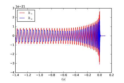
Figure 1: The waveform polarizations $h_{+}$(red) and $h_{\times}$(blue) of the publicly available SXS waveform SXS:BBH:0006 generated via the waveform interface in lalsimulation (left panel) and constructed using scipy’s UnivariateSpline function(right panel).

IV LAL coordinate frames for precessing binaries and NR injections

IV.0.1 Executive summary: changes of conventions

It has recently became apparent that certain waveform conventions in LAL are not ideal to specify precessing binaries: (i) The phase-angle phiRef couples the specification of the line-of-sight to Earth with the specification of spin components S1x, S1y, S1z, S2x, S2y, S2z. To compute waveforms for the identical compact binary viewed from different directions, one may have to specify different values for the spin-components S1x, S1y, S2x, S2y. (ii) Several semi-analytic waveform models do not conform to this convention, already following the convention detailed below.

Concretely, the spin-components are now specified in a geometric way based on the angular momentum $\hat{L}$ and the line connecting object 2 to object 1, $\hat{n}$:

S1x $$\overset{\rm ref}{=}\vec{\chi}_{1}\cdot\hat{n},$$ (5)

S1y $$\overset{\rm ref}{=}\vec{\chi}_{1}\cdot(\hat{L}\times\hat{n}),$$ (6)

S1z $$\overset{\rm ref}{=}\vec{\chi}_{1}\cdot\hat{L},$$ (7)

(and similarly for the second object). The symbol $\overset{\rm ref}{=}$ indicates that equality only holds at a reference time as spins generically precess during an inspiral Apostolatos et al. (1994); Kidder (1995).

Furthermore, it is suggested to specify orientation of eccentric orbits through the angles

$$\mbox{\tt phiRef}=\Phi \overset{\rm ref}{=}\angle(\hat{n},\mbox{line-of-ascending-node}),$$ (8)

$$\mbox{\tt mean\_anomaly}=\delta.$$ (9)

IV.0.2 Motivation & benefits of new conventions

Generally waveform modeling requires at least two coordinate systems, a “source-frame” in which it is convenient to specify properties of the source of gravitational waves, and a “wave-frame” which is adopted to wave-propagation to GW detectors on Earth. Furthermore, NR data are specified in whatever coordinates are employed during the numerical evolution, generally resulting in a third coordinate system. This section defines coordinate frames for use in LAL. Specifically, we achieve:

1. Identification of a set of intrinsic parameters that fully describe the dynamics of a binary on an eccentric orbit, defined solely in terms of the source-frame (i.e. independent of the wave-frame).

2. Identification of three angles that describe the transformation between source- and wave-frame, which are independent of the intrinsic parameters.

3. Identification of parameters describing the orbital phase and periapsis location, which have a convenient circular-orbit limit: As the eccentricity tends to zero, one of the two phase-parameters reduces to the standard orbital phase for circular orbits, whereas the other becomes irrelevant.

4. Identities that relate the basis-vectors in the source-frame to the wave-frame (and vice versa). These identities are written in vectorial form and are valid in any coordinate system.

The orthogonal decomposition into intrinsic and extrinsic parameters (points 1 and 2) allows to change the direction at which a binary is viewed (i.e. the wave-frame), without having to adjust the parameters that determine the intrinsic dynamics. Point 3 prepares the ground for easy extension to eccentric waveforms. point 4 is of particular relevance when translating NR data into LAL-conventions: Evaluating the vector identities in the NR-coordinate system, yields immediately the relation between NR coordinates and wave-frame.

IV.0.3 NR waveform injections

NR data are assumed to be supplied in the data-format defined in Sec. II and III, and so it needs to be transformed into the LAL wave-frame. For a given reference time, an entire NR data-set could in principle be transformed into the LAL frame by suitably transforming each $H_{\ell m}$-mode. Applying such a coordinate transformation on the NR-data as a pre-processing step before using it for injections suffers from two disadvantages: First, the person who prepares the NR-data for LAL-use must perform the rotation, and must do so correctly. Since NR data is prepared separately by several NR groups, this opens the possibility of introducing errors in this step. Secondly, for precessing systems the orbital angular momentum $\hat{L}$ precesses. Therefore, pre-rotating the NR-data locks in the reference point, and one would need to generate different pre-transformed NR-data for different reference points. Since NR data is in geometric units, the NR-data would have to be separately transformed whenever the total mass of an injection changes.

To avoid both disadvantages, it is proposed to leave the NR-data in its original frame (see Sec. II). Instead, the transformations between the LAL-convention and the NR-data are applied at use during the call to the waveform evaluation function in LAL (cf. Sec. III).

This section develops the necessary transformations to implement this technique. No assumptions are made on the NR-coordinate system in order to allow for precession when NR-orbital angular momentum is typically not along the z-axis of the NR-coordinate system. The derived formulae also allow to choose an arbitrary reference point for the NR waveform, as long as orbital angular momentum and vector connecting the two compact objects are known at that point.

IV.1 Coordinate frames

The frames defined here differ somewhat from the preceding LAL conventions as detailed in ins . The differences are needed to achieve the separation between intrinsic and extrinsic parameters. In the old conventions, the orbital phase $\phi$ was also used as part of the rotation parameters that define the rotation between source- and wave-frame. Therefore, to “look” at the same binary from different angles used to require a suitable change in the spin-components tangential to the orbital plane.

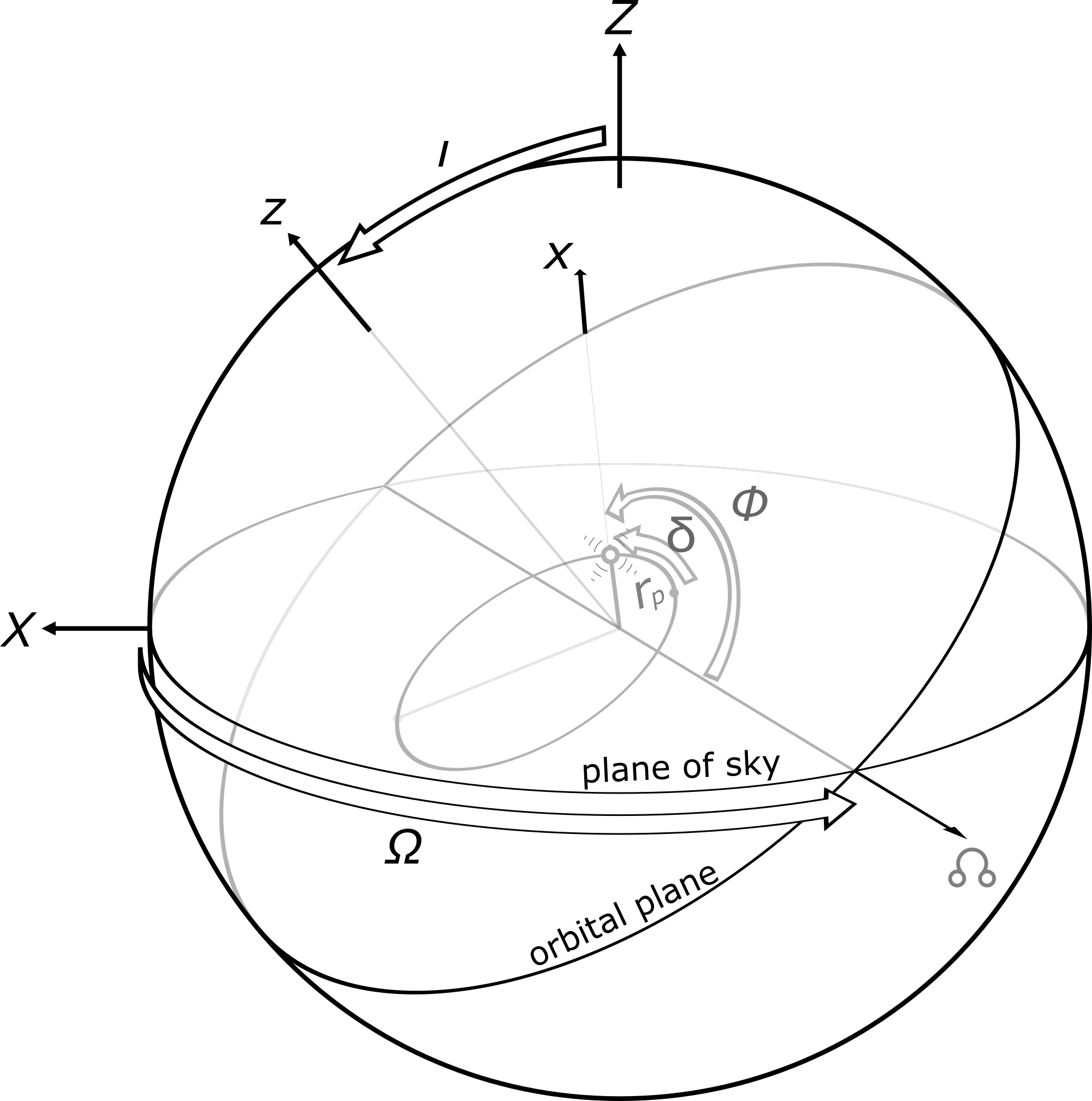
Figure 2: Coordinate frames. (x,y,z) denotes the source-frame and (X,Y,Z) the wave-frame. For the recommended default $\Omega=\pi/2$, the line of ascending nodes agrees with $\hat{Y}$ i.e. the rotation by the inclination angle $\iota$ is about the $\hat{Y}$-axis.

IV.1.1 NR frame $(\hat{e}_{x},\hat{e}_{y},\hat{e}_{z})$

This is a generic coordinate system without any regards to the concrete binary motion. Generic coordinate systems occur in numerical relativity, where the coordinates are chosen through some gauge-conditions, and the binary is evolving from some initial data. At some later time therefore, the coordinates will not have any particular, controlled properties. The Cartesian basis-vectors are denoted

$$\hat{e}_{x},\hat{e}_{y},\hat{e}_{z}.$$ (10)

From these, spherical basis-vectors can be computed as

$${\hat{r}} =\cos\phi\sin\theta\;\hat{e}_{x}+\sin\phi\sin\theta\;\hat{e}_{y}+\cos\theta\;\hat{e}_{z}$$ (11a)

$${\hat{\theta}} =\cos\phi\cos\theta\;\hat{e}_{x}+\sin\phi\cos\theta\;\hat{e}_{y}-\sin\theta\;\hat{e}_{z}$$ (11b)

$${\hat{\phi}} =-\sin\phi\;\hat{e}_{x}+\cos\phi\;\hat{e}_{y}.$$ (11c)

NR data are assumed to be represented by spherical-harmonic modes of the NR coordinates, as previously defined in the NINJA data-formats document Brown et al. (2007):

$$h_{+}^{\rm NR}(t_{\rm GW}) =\frac{1}{2}\left({\hat{\theta}}_{i}{\hat{\theta}}_{j}-{\hat{\phi}}_{i}{\hat{\phi}}_{j}\right)h^{ij}(t_{\rm GW})$$ (12a)

$$h_{\times}^{\rm NR}(t_{\rm GW}) =\frac{1}{2}\left({\hat{\theta}}_{i}{\hat{\phi}}_{j}+{\hat{\phi}}_{i}{\hat{\theta}}_{j}\right)h^{ij}(t_{\rm GW}),$$ (12b)

and

$$\sum_{\ell=2}^{\infty}\sum_{m=-\ell}^{\ell}H_{\ell m} (t_{\rm GW})\;^{-2}Y_{\ell m}(\theta,\phi)=\frac{r}{M}\Big{(}h_{+}^{\rm NR}(t_{\rm GW})-ih_{\times}^{\rm NR}(t_{\rm GW})\Big{)}.$$ (13)

As explained in Sec. II, the data-files are assumed to contain a compressed time-series of amplitudes and phases per Eq. (3). Given an emission direction $(\theta,\phi)$, Eq. (13) yields the GW modes $h_{+}^{\rm NR}(t_{\rm GW})$ and $h_{\times}^{\rm NR}(t_{\rm GW})$, according to the convention Eqs. (12).

The gravitational wave data are given in a time-coordinate $t_{\rm GW}$ of observers at large distance r.

Let us now turn to a description of the dynamics of the two bodies. Numerical relativity defines a variety of vectors, the combination of which defines the instantaneous state of the two bodies. These are: The dimensionless spin vectors of the two bodies,

$$\vec{\chi}_{1}(t),\,\vec{\chi}_{2}(t);$$ (14)

the direction from body 2 to body 1,

$$\hat{n}(t):=\frac{\vec{c}_{1}-\vec{c}_{2}}{||\vec{c}_{1}-\vec{c}_{2}||},$$ (15)

where $\vec{c}_{i}$ is the coordinate centre of the horizon of the i-th body; the direction of the Newtonian orbital angular momentum,

$$\hat{L}_{N}(t).$$ (16)

We do not make any assumption about the relation of the NR orbital angular momentum vector $\hat{L}$ relative to the NR coordinates. One can further define an orbital frequency

$$\vec{\Omega}_{\mathrm{orb}}(t)=\hat{n}(t)\times\frac{d\hat{n}(t)}{dt}.$$ (17)

Equations (14)–(17) are defined in the strong-field region near the black holes, and are given as a function of the time-coordinate $t$ employed by the NR simulation in the strong field regime. The time-coordinates $t_{\rm GW}$ and $t$ are defined at different regions of the space-time (far-zone vs. near-zone), and their preferred relative alignment is discussed on page II.3. Any relation between $t_{\rm GW}$ and $t$, however, is ambiguous. Often NR simulations employ an approximation of “retarded time”, i.e.

$$t_{\rm GW}=t\big{|}_{\rm retarded}.$$ (18)

However, in a dynamical space-time with black holes, two difficulties arise: First, the horizons are causally disconnected from future null infinity, so there are no outgoing null-rays that connect the horizons to the wave-zone. Secondly, when integrating null-rays “slightly outside” the horizons, the time-delay to infinity will depend on precisely where the integration was started, as well as on the initial direction of the null-ray. Therefore, any relation between $t_{\rm GW}$ and $t$ should be viewed as approximate. One should further assume that different NR groups may use different definitions of $t_{\rm GW}$ in the data they compute.

IV.1.2 LAL Source-Frame $({{\hat{x}}},{{\hat{y}}},{{\hat{z}}})$

The LAL source-frame $({{\hat{x}}},{{\hat{y}}},{{\hat{z}}})$ is defined as follows:

1. The ${{\hat{z}}}$-axis points along the orbital angular momentum of the binary,

   $${{\hat{z}}}\overset{\rm ref}{=}\hat{L}.$$ (19)

2. The ${{\hat{x}}}$-axis points along the vector $\hat{n}$ pointing from the second to the first body,

   $${{\hat{x}}}\overset{\rm ref}{=}\hat{n}.$$ (20)

3. The third vector ${{\hat{y}}}={{\hat{z}}}\times{{\hat{x}}}$ completes the triad.

The symbol $\overset{\rm ref}{=}$ indicates that the respective equation is only required at the reference epoch. The reference epoch can be unambiguously specified by a reference-time $t_{\rm ref}$. One can also specify a reference orbital frequency $\Omega_{\rm orb,ref}$, and infer $t_{\rm ref}$ via Eq. (17), $\Omega_{\rm orb}(t_{\rm ref})=\Omega_{\rm orb,ref}$. If the reference epoch is desired to be specified in terms of a gravitational wave–frequency, then the gravitational wave time $t_{\rm GW}$ needs to be related to the time-coordinate of the black hole dynamics, $t$. As discussed in the context of Eq. (18), such an identification is ambiguous and holds only approximately.

Equations (19) and (20) define the source-frame at the reference epoch only. They are chosen such that the spin-components (Sx1, Sy1, Sz1) and (S2x, S2y, S2z) have coordinate-invariant meaning: Sx1 is the projection of $\vec{\chi}_{1}$ onto $\hat{n}$, Sz1 is the projection of $\vec{\chi}_{1}$ onto $\hat{L}$, etc.

The source-frame does not rotate as the binary evolves. Specifically, the rotation between source-frame and wave-frame described below is constant in time.

A different reference epoch would lead to a different source-frame, related by some rotation. If the reference epoch is shifted by a small amount (comparable to the orbital time-scale), ${{\hat{x}}}$ and ${{\hat{y}}}$ would rotate with the binary. On the precession time-scale ${{\hat{z}}}$ would change.

The source frame has no deep intrinsic, geometric significance. It is merely a vehicle to describe the spin-projections onto intrinsic geometric directions, and the basis-vectors $({{\hat{x}}},{{\hat{y}}},{{\hat{z}}})$ will be convenient when writing down the transformation to the wave-frame.

IV.1.3 Intrisinc parameters of a binary

Given a reference epoch, a binary is specified by the following ten numbers:

• Two masses $m_{1}$, $m_{2}$.

• Two spin-vectors $\vec{\chi}_{1}$, $\vec{\chi}_{2}$, specified through the projections of the spin-vectors onto $\hat{L}$, $\hat{n}$ and the third basis-vector (at reference time).

• Eccentricity $e$.

• Mean anomaly $\delta$. The mean anomaly is defined in terms of the current time $t$, the time of last periapsis passage $T_{\rm previous}$, and the time of next periapsis passage $T_{\rm next}$:

  $$\delta=2\pi\frac{t-T_{\rm previous}}{T_{\rm next}-T_{\rm previous}}.$$ (21)

Eccentricity should be defined somehow “near” the reference epoch. A precise definition (if possible at all) is left to the future. For low eccentricity orbits, there is a competition between radiation reaction driven inspiral (which results in a slightly negative average radial velocity), and the oscillatory radial motion due to eccentricity. For sufficiently small eccentricity, minima in separation may no longer exist. If mean anomaly is still needed despite the quite low eccentricity in such cases, one will have to define periapsis as minimum of separation compared to a fiducial smooth inspiral trajectory.

IV.1.4 Wave-Frame $(\hat{X},\hat{Y},\hat{Z})$

The wave-frame is adopted to the direction of the observer (i.e. Earth), such that its $\hat{Z}$-axis points toward the observer. $\hat{X}$ and $\hat{Y}$ represent basis-vectors orthogonal to the line-of-sight, i.e. they span the plane of the sky. The wave-frame is completely specified by three angles:

1. The angle $\Phi$ between line of ascending node and $\hat{n}$ (at the reference time).

2. The inclination $\iota$, i.e. the angle between orbital angular momentum $\hat{L}={{\hat{z}}}$ and the line-of-sight $\hat{Z}$.

3. The angle $\Omega$ between the $\hat{X}$-axis and the line of the ascending node (at the reference time).

These three angles happen to be the Euler angles of the rotation from the wave-frame to the source-frame. In the LAL wave-frame, the gravitational wave modes are defined as

$$h_{+}^{\rm W} =\frac{1}{2}\left(\hat{X}_{i}\hat{X}_{j}-\hat{Y}_{i}\hat{Y}_{j}\right)h^{ij},$$ (22a)

$$h_{\times}^{\rm W} =\frac{1}{2}\left(\hat{X}_{i}\hat{Y}_{j}+\hat{Y}_{i}\hat{X}_{j}\right)h^{ij},$$ (22b)

where the superscript ’W’ indicates the LAL wave-frame. The angle $\Omega$ rotates $\hat{X}$ and $\hat{Y}$ into each other. By definition of Eq. (22), this merely rotates the polarization of the GW modes, and so $\Omega$ is fully degenerate with the GW polarization.

Note that the phase-angle $\Phi$ is specified without regard to the location of periapsis of the binary (this differs from the previous LAL convention). This new definition decouples the specification of periapsis location and the specification of orbital phase, and avoids the ambiguity that would arise in the zero-eccentricity limit of definitions involving periapsis. Indeed, for fixed $\Phi$ and fixed $\delta$, as eccentricity approaches zero, the waveforms will approach the identical circular form, independent of the value of $\delta$.

IV.2 Relationship between frames

IV.2.1 From source-frame to wave-frame

The relation between source-frame and wave-frame can be easily derived following the three rotations that rotate one frame into the other: Beginning in the source-frame, ${{\hat{x}}},{{\hat{y}}},{{\hat{z}}}$, we first apply the rotation by $\Phi$ around ${{\hat{z}}}$, which yields a frame with basis-vectors $\hat{p},\hat{q},{{\hat{z}}}$:

$$\hat{p} =\cos\Phi\,{{\hat{x}}}-\sin\Phi\,{{\hat{y}}},$$ (23a)

$$\hat{q} =\sin\Phi\,{{\hat{x}}}+\cos\Phi\,{{\hat{y}}},$$ (23b)

$${{\hat{z}}} ={{\hat{z}}}.$$ (23c)

The inverse rotation is

$${{\hat{x}}} =\;\;\;\cos\Phi\,\hat{p}+\sin\Phi\,\hat{q},$$ (24a)

$${{\hat{y}}} =-\sin\Phi\,\hat{p}+\cos\Phi\,\hat{q},$$ (24b)

$${{\hat{z}}} ={{\hat{z}}}.$$ (24c)

The vectors $\hat{p},\hat{q}$ form an orthonormal basis of the ${{\hat{x}}}$-${{\hat{y}}}$ plane, such that $\hat{p}$ points in the direction of ascending node.
Next, we rotate around the line of the ascending node by the inclination $\iota$, resulting in basis-vectors

$$\hat{P} =\hat{p},$$ (25a)

$$\hat{Q} =\cos\iota\,\hat{q}-\sin\iota\,{{\hat{z}}},$$ (25b)

$$\hat{Z} =\sin\iota\,\hat{q}+\cos\iota\,{{\hat{z}}}.$$ (25c)

$\hat{P}$ and $\hat{Q}$ form an orthonormal basis of the $\hat{X}$-$\hat{Y}$-plane with $\hat{P}$ pointing in the direction of the ascending node. The inverse rotation is

$$\hat{p} =\hat{P},$$ (26a)

$$\hat{q} =\;\;\;\cos\iota\,\hat{Q}+\sin\iota\,\hat{Z},$$ (26b)

$${{\hat{z}}} =-\sin\iota\,\hat{Q}+\cos\iota\,\hat{Z}.$$ (26c)

The final rotation rotates $\hat{P}$ and $\hat{Q}$ around $\hat{Z}$ into $\hat{X},\hat{Y}$:

$$\hat{X} =\cos\Omega\,\hat{P}-\sin\Omega\,\hat{Q},$$ (27a)

$$\hat{Y} =\sin\Omega\,\hat{P}+\cos\Omega\,\hat{Q},$$ (27b)

$$\hat{Z} =\hat{Z}.$$ (27c)

The inverse rotation is

$$\hat{P} =\;\;\;\cos\Omega\,\hat{X}+\sin\Omega\,\hat{Y},$$ (28a)

$$\hat{Q} =-\sin\Omega\,\hat{X}+\cos\Omega\,\hat{Y},$$ (28b)

$$\hat{Z} =\hat{Z}.$$ (28c)

Substituting Eqs. (23), (25) and (27) into each other, one obtains the entire transformation:

$$\hat{X}= \left(\cos\Omega\cos\Phi-\sin\Omega\cos\iota\sin\Phi\right){{\hat{x}}}$$

$$+\left(-\cos\Omega\sin\Phi-\sin\Omega\cos\iota\cos\Phi\right){{\hat{y}}}$$

$$+\sin\Omega\sin\iota\,{{\hat{z}}},$$ (29a)

$$\hat{Y}= \left(\sin\Omega\cos\Phi+\cos\Omega\cos\iota\sin\Phi\right){{\hat{x}}}$$

$$+\left(-\sin\Omega\sin\Phi+\cos\Omega\cos\iota\cos\Phi\right){{\hat{y}}}$$

$$-\cos\Omega\sin\iota\,{{\hat{z}}},$$ (29b)

$$\hat{Z}= \sin\iota\sin\Phi\,{{\hat{x}}}+\sin\iota\cos\Phi\,{{\hat{y}}}+\cos\iota\,{{\hat{z}}}.$$ (29c)

The inverse transformation is obtained from Eqs. (24), (26) and (28):

$${{\hat{x}}}= \left(\cos\Omega\cos\Phi-\sin\Omega\cos\iota\sin\Phi\right)\hat{X}$$

$$+\left(\sin\Omega\cos\Phi+\cos\Omega\cos\iota\sin\Phi\right)\hat{Y}$$

$$+\sin\iota\sin\Phi\,\hat{Z},$$ (30a)

$${{\hat{y}}}= \left(-\cos\Omega\sin\Phi-\sin\Omega\cos\iota\cos\Phi\right)\hat{X}$$

$$+\left(-\sin\Omega\sin\Phi+\cos\Omega\cos\iota\cos\Phi\right)\hat{Y}$$

$$+\sin\iota\cos\Phi\,\hat{Z},$$ (30b)

$${{\hat{z}}}= \sin\Omega\sin\iota\,\hat{X}-\cos\Omega\sin\iota\,\hat{Y}+\cos\iota\,\hat{Z}.$$ (30c)

Equation (30c) shows that $\Omega$ determines the direction of $\hat{L}=\hat{z}$ on the plane of the sky. For $\Omega=0$, $\hat{L}$ lies in the $\hat{Y}$-$\hat{Z}$ plane, and for $\Omega=\pi/2$, it lies in the $\hat{X}$-$\hat{Z}$ plane. This latter choice ($\Omega=\pi/2$) is already respected by many LAL waveform models. Therefore, in the absence of a reason to do otherwise, all waveform models should default to $\Omega=\pi/2$.
With this recommended default $\Omega=\pi/2$, Eqs. (29) simplify to

$$\hat{X}= -\cos\iota\sin\Phi\,{{\hat{x}}}-\cos\iota\cos\Phi\,{{\hat{y}}}\,+\sin\iota\,{{\hat{z}}},$$ (31a)

$$\hat{Y}= \quad\quad\;\;\;\cos\Phi\,{{\hat{x}}}\qquad\,-\sin\Phi\,{{\hat{y}}},$$ (31b)

$$\hat{Z}= \;\;\;\;\,\sin\iota\sin\Phi\,{{\hat{x}}}+\sin\iota\cos\Phi\,{{\hat{y}}}\,+\cos\iota\,{{\hat{z}}}.$$ (31c)

The inverse transformation (30) simplifies to

$${{\hat{x}}}= -\cos\iota\sin\Phi\,\hat{X}+\cos\Phi\,\hat{Y}+\sin\iota\sin\Phi\,\hat{Z},$$ (32a)

$${{\hat{y}}}= -\cos\iota\cos\Phi\,\hat{X}-\sin\Phi\,\hat{Y}+\sin\iota\cos\Phi\,\hat{Z},$$ (32b)

$${{\hat{z}}}= \qquad\quad\;\,\sin\iota\,\hat{X}\qquad\qquad\qquad\;+\cos\iota\,\hat{Z}.$$ (32c)

IV.2.2 From NR-frame to wave-frame

Equations (29) and (31) are of particular importance. By definition, the source-frame basis-vectors are trivially related to vectorial quantities of the compact binary dynamics:

$${{\hat{x}}} \overset{\rm ref}{=}\hat{n},$$ (33a)

$${{\hat{y}}} \overset{\rm ref}{=}(\hat{L}\times\hat{n}),$$ (33b)

$${{\hat{z}}} \overset{\rm ref}{=}\hat{L}.$$ (33c)

Therefore, if the dynamics vectors $\hat{L}$ and $\hat{n}$ are known in any coordinate system, e.g. the NR coordinates, then Eqs. (29) yield the wave-frame basis-vectors in those coordinates. Specifically, for $\Omega=\pi/2$, Eqs. (31) yield

$$\hat{X} \overset{\rm ref}{=}-\cos\iota\left[\sin\Phi\,\hat{n}+\cos\Phi\,\hat{L}\times\hat{n}\right]+\sin\iota\hat{L},$$ (34a)

$$\hat{Y} \overset{\rm ref}{=}\qquad\quad\;\,\cos\Phi\,\hat{n}-\sin\Phi\,\hat{L}\times\hat{n},$$ (34b)

$$\hat{Z} \overset{\rm ref}{=}\;\;\;\;\sin\iota\left[\sin\Phi\,\hat{n}+\cos\Phi\,\hat{L}\times\hat{n}\right]+\cos\iota\,\hat{L}.$$ (34c)

Let us consider next the transformation of the GW strain polarizations from the generic (NR) frame Eq. (11) to the wave-frame. $\hat{X}$ and $\hat{Y}$ are orthogonal to the direction of propagation $\hat{Z}={\hat{r}}$ of the gravitational wave. Therefore, $({\hat{\theta}},{\hat{\phi}})$ can be rotated into $(\hat{X},\hat{Y})$ through a rotation by an angle $\alpha$:

$$\hat{X} =\cos\alpha\,{\hat{\theta}}-\sin\alpha\,{\hat{\phi}},$$ (35a)

$$\hat{Y} =\sin\alpha\,{\hat{\theta}}+\cos\alpha\,{\hat{\phi}}.$$ (35b)

Substituting Eqs. (35) into Eqs. (22) we can compute $h_{+}^{\rm W}$ and $h_{\times}^{\rm W}$ in terms of $({\hat{\theta}},{\hat{\phi}})$. Comparing further with Eqs. (12), we find:

$$h_{+}^{\rm W}(t_{\rm GW}) =\cos\left(2\alpha\right)\,h_{+}^{\rm NR}(t_{\rm GW})-\sin\left(2\alpha\right)\,h_{\times}^{\rm NR}(t_{\rm GW}),$$ (36a)

$$h_{\times}^{\rm W}(t_{\rm GW}) =\sin(2\alpha)\,h_{+}^{\rm NR}(t_{\rm GW})+\cos\left(2\alpha\right)\,h_{\times}^{\rm NR}(t_{\rm GW}).$$ (36b)

Not surprising, the GW polarizations in the wave-frame are obtained from those in the NR-frame by a rotation of $2\alpha$.

The wave-frame $\hat{X},\hat{Y}$ depend on $\Omega$, and therefore $h_{+}^{\rm W}$ and $h_{\times}^{\rm W}$ also depend on $\Omega$. We can make this dependence explicit by resorting to the intermediate vectors $\hat{P}$ and $\hat{Q}$. These are also orthogonal to $\hat{Z}$, therefore they, too, can be obtained from ${\hat{\theta}}$ and ${\hat{\phi}}$ by a rotation:

$$\hat{P} =\cos\alpha^{\prime}\,{\hat{\theta}}-\sin\alpha^{\prime}\,{\hat{\phi}},$$ (37a)

$$\hat{Q} =\sin\alpha^{\prime}\,{\hat{\theta}}+\cos\alpha^{\prime}\,{\hat{\phi}}.$$ (37b)

However, $\hat{P}$ and $\hat{Q}$ are independent of $\Omega$ and therefore, $\alpha^{\prime}$ is independent of $\Omega$. Because $(\hat{X},\hat{Y})$ are rotated by $\Omega$ relative to $(\hat{P},\hat{Q})$, we have

$$\alpha=\Omega+\alpha^{\prime}.$$ (38)

Because rotations add, we can therefore write

$$\left(\begin{aligned} h_{+}^{\rm W}\\ h_{\times}^{\rm W}\end{aligned}\right)={\mathbf{R}}_{2\Omega}\;{\mathbf{R}}_{2\alpha^{\prime}}\left(\begin{aligned} h_{+}^{\rm NR}\\ h_{\times}^{\rm NR}\end{aligned}\right),$$ (39)

where ${\mathbf{R}}_{\beta}$ denotes a 2x2 rotation matrix,

$${\mathbf{R}}_{\beta}=\left(\begin{aligned} &\cos\beta&-\sin\beta\\ &\sin\beta&\cos\beta\end{aligned}\right).$$ (40)

Equation (39) thus implies that the waveform-modes are obtained from the NR-polarizations by (i) applying an $\Omega$-independent rotation by $2\alpha^{\prime}$; followed by (ii) a rotation by $2\Omega$. For $\Omega=\pi/2$, we have ${\mathbf{R}}_{\pi}=-{\mathbf{1}}$. Therefore, between $\Omega=0$ (inclination rotated about X-axis) and $\Omega=\pi/2$ (inclination rotated about Y-axis), the waveform polarization pick up precisely an overall minus-sign.

IV.3 Computing GW polarizations in the LAL wave-frame

Let us finally write down explicit instructions of how to obtain GW polarizations in the LAL convention, given NR waveform data. Given parameters i, phiRef passed into XLALSimInspiralChooseTDWaveform, proceed as follows:

1. Define $\Phi=\mbox{phiRef}$, $\iota={\tt i}$.

2. Compute $\hat{Z}_{\rm ref}$ at the reference time by evaluating Eq. (34c).

3. Because $\hat{Z}$ points in the direction of emission of the gravitational wave, we must have

   $$\hat{Z}_{\rm ref}\overset{\rm ref}{=}\left(\begin{gathered}\cos\phi\sin\theta\\ \sin\phi\sin\theta\\ \cos\theta\end{gathered}\right).$$ (41)

   From this equality, read off $(\theta,\phi)$. Then compute the NR-basis vectors ${\hat{\theta}},{\hat{\phi}}$ from Eqs. (11).

4. If $\Omega=\pi/2$, compute $\sin\alpha$ and $\cos\alpha$ by taking inner products of Eq. (35b) with ${\hat{\theta}}$ and ${\hat{\phi}}$:

   $$\sin\alpha =\cos\Phi\,\hat{n}\cdot{\hat{\theta}}-\sin\Phi\,(\hat{L}\times\hat{n})\cdot{\hat{\theta}},$$ (42a)

   $$\cos\alpha =\cos\Phi\,\hat{n}\cdot{\hat{\phi}}-\sin\Phi\,(\hat{L}\times\hat{n})\cdot{\hat{\phi}}.$$ (42b)

   If $\Omega\neq\pi/2$, compute instead inner products based on Eqs. (29).

5. Substitute $(\theta,\phi)$ into Eqs. (13) and (12) to compute $h_{+}^{\rm NR}(t_{\rm GW})$ and $h_{\times}^{\rm NR}(t_{\rm GW})$.

6. Compute $\cos 2\alpha=\cos^{2}\alpha\!-\!\sin^{2}\alpha$ and $\sin 2\alpha=2\cos\alpha\sin\alpha$. Substitute into Eqs. (36) to compute $h_{+}^{\rm W}(t_{\rm GW})$ and $h_{\times}^{\rm W}(t_{\rm GW})$.

IV.3.1 Evaluate spin-consistency in LAL source-frame

The parameters S1x, S1y, S1z, S2x, S2y,S2z passed into LALSimInspiralChooseTDWaveform are supposed to be the LAL source-frame parameters, i.e. these parameters should simply be the projections of $\vec{\chi}_{1,2}$ onto the source-frame basis-vectors $({{\hat{x}}},{{\hat{y}}},{{\hat{z}}})$. Substituting Eqs. (19) and (20), one arrives at the following consistency conditions:

S1x $$\overset{\rm ref}{=}\vec{\chi}_{1}\cdot\hat{n},$$ (43a)

S1y $$\overset{\rm ref}{=}\vec{\chi}_{1}\cdot(\hat{L}\times\hat{n}),$$ (43b)

S1z $$\overset{\rm ref}{=}\vec{\chi}_{1}\cdot\hat{L}.$$ (43c)

The conditions for body 2 are obtained by $1\leftrightarrow 2$.

V Discussion

With this new infrastructure it is very easy and much less memory intensive to use NR waveforms directly for data analysis applications. The “NR_hdf5” approximant works much the same as any other approximant in lalsimulation but there are a few important differences.

First, the user must supply the location of the HDF5 file, a functionality which was already implemented for NINJA, but was not previously used in lalsimulation. Secondly, the user must be careful to supply the mass ratio and spin values that are consistent with the NR files, and the spin values have to be specified in the LAL source frame (see Eqs. (43)).

The current implementation still suffers from a few caveats and drawbacks. As opposed to the continuous waveform approximants, at the moment the metadata are only referring to the beginning of the waveform and not some reference time, which can be chosen freely. While this is not a problem for aligned-spin binaries, this is a big concern for precessing simulations since various quantities, in particular the spins and the orbital angular momentum, are time-dependent. To fully integrate this desired freedom, additional information needs to be incorporated into the HDF5 files and the waveform evaluation functions accordingly. Specifically, one needs the time-series of the vectors determining the geometry of the binary: $\hat{L}(t),\hat{n}(t),\chi_{(}t),\chi_{2}(t)$. Given these time-series, one can interpolate these four vectors to any reference epoch, and then apply the frame transformations at this reference epoch. These are provided in the formats 2 and 3 and we leave it to future upgrades to lalsimulation to allow for this additional functionality to be fully integrated in the waveform evaluation functions.

References

- Abbott et al. (2016a) B. P. Abbott et al. (Virgo, LIGO Scientific), Phys. Rev. Lett. 116, 061102 (2016a), eprint 1602.03837.
- Abbott et al. (2016b) B. P. Abbott et al. (Virgo, LIGO Scientific), Phys. Rev. Lett. 116, 241103 (2016b), eprint 1606.04855.
- Abbott et al. (2016c) B. P. Abbott et al. (Virgo, LIGO Scientific), Phys. Rev. X6, 041015 (2016c), eprint 1606.04856.
- Sathyaprakash and Schutz (2009) B. S. Sathyaprakash and B. F. Schutz, Living Rev. Rel. 12, 2 (2009), eprint 0903.0338.
- Blanchet (2014) L. Blanchet, Living Reviews in Relativity 17 (2014), URL http://www.livingreviews.org/lrr-2014-2.
- Pretorius (2005) F. Pretorius, Phys. Rev. Lett. 95, 121101 (2005), eprint gr-qc/0507014.
- Baker et al. (2006) J. G. Baker, J. Centrella, D.-I. Choi, M. Koppitz, and J. van Meter, Phys. Rev. Lett. 96, 111102 (2006), eprint gr-qc/0511103.
- Campanelli et al. (2006) M. Campanelli, C. O. Lousto, P. Marronetti, and Y. Zlochower, Phys. Rev. Lett. 96, 111101 (2006), eprint gr-qc/0511048.
- Centrella et al. (2010) J. Centrella, J. G. Baker, B. J. Kelly, and J. R. van Meter, Rev. Mod. Phys. 82, 3069 (2010), eprint 1010.5260.
- Ohme (2012) F. Ohme, Class. Quant. Grav. 29, 124002 (2012), eprint 1111.3737.
- Hannam et al. (2014) M. Hannam, P. Schmidt, A. Boh , L. Haegel, S. Husa, F. Ohme, G. Pratten, and M. P rrer, Phys. Rev. Lett. 113, 151101 (2014), eprint 1308.3271.
- Pan et al. (2014) Y. Pan, A. Buonanno, A. Taracchini, L. E. Kidder, A. H. Mrou , H. P. Pfeiffer, M. A. Scheel, and B. Szil gyi, Phys. Rev. D89, 084006 (2014), eprint 1307.6232.
- Taracchini et al. (2014) A. Taracchini et al., Phys. Rev. D89, 061502 (2014), eprint 1311.2544.
- Khan et al. (2016) S. Khan, S. Husa, M. Hannam, F. Ohme, M. Pürrer, X. Jim nez Forteza, and A. Boh , Phys. Rev. D93, 044007 (2016), eprint 1508.07253.
- Healy et al. (2014) J. Healy, C. O. Lousto, and Y. Zlochower, Phys. Rev. D90, 104004 (2014), eprint 1406.7295.
- Abbott et al. (2016d) B. P. Abbott et al. (Virgo, LIGO Scientific) (2016d), eprint 1611.07531.
- Aylott et al. (2009) B. Aylott et al., Class. Quant. Grav. 26, 165008 (2009), eprint 0901.4399.
- Aasi et al. (2014) J. Aasi et al. (VIRGO, LIGO Scientific, NINJA-2), Class. Quant. Grav. 31, 115004 (2014), eprint 1401.0939.
- Galley and Schmidt (2016) C. R. Galley and P. Schmidt (2016), eprint 1611.07529.
- Newman and Penrose (1962) E. Newman and R. Penrose, J. Math. Phys. 3, 566 (1962).
- Penrose (1963) R. Penrose, Phys. Rev. Lett. 10, 66 (1963).
- Regge and Wheeler (1957) T. Regge and J. A. Wheeler, Phys. Rev. 108, 1063 (1957).
- Zerilli (1970a) F. J. Zerilli, Phys. Rev. Lett. 24, 737 (1970a).
- Zerilli (1970b) F. J. Zerilli, Phys. Rev. D2, 2141 (1970b).
- Moncrief (1974) V. Moncrief, Annals Phys. 88, 323 (1974).
- (26) C. R. Galley, romSpline, URL https://bitbucket.org/chadgalley/romspline.
- Brown et al. (2007) D. Brown, S. Fairhurst, B. Krishnan, R. A. Mercer, R. K. Kopparapu, L. Santamaria, and J. T. Whelan (2007), eprint 0709.0093.
- Fiske et al. (2005) D. R. Fiske, J. G. Baker, J. R. van Meter, D.-I. Choi, and J. M. Centrella, Phys. Rev. D71, 104036 (2005), eprint gr-qc/0503100.
- Boyle and Mroue (2009) M. Boyle and A. H. Mroue, Phys. Rev. D80, 124045 (2009), eprint 0905.3177.
- Dal Canton et al. (2014) T. Dal Canton et al., Phys. Rev. D90, 082004 (2014), eprint 1405.6731.
- Mroue et al. (2013) A. H. Mroue et al., Phys. Rev. Lett. 111, 241104 (2013), eprint 1304.6077.
- Apostolatos et al. (1994) T. A. Apostolatos, C. Cutler, G. J. Sussman, and K. S. Thorne, Phys. Rev. D49, 6274 (1994).
- Kidder (1995) L. E. Kidder, Phys. Rev. D52, 821 (1995), eprint gr-qc/9506022.
- (34) URL http://software.ligo.org/docs/lalsuite/lalsimulation/group__lalsimulation__inspiral.html.