Gauging Variational Inference

Abstract

Computing partition function is the most important statistical inference task arising in applications of Graphical Models (GM). Since it is computationally intractable, approximate methods have been used to resolve the issue in practice, where mean-field (MF) and belief propagation (BP) are arguably the most popular and successful approaches of a variational type. In this paper, we propose two new variational schemes, coined Gauged-MF (G-MF) and Gauged-BP (G-BP), improving MF and BP, respectively. Both provide lower bounds for the partition function by utilizing the so-called gauge transformation which modifies factors of GM while keeping the partition function invariant. Moreover, we prove that both G-MF and G-BP are exact for GMs with a single loop of a special structure, even though the bare MF and BP perform badly in this case. Our extensive experiments, on complete GMs of relatively small size and on large GM (up-to 300 variables) confirm that the newly proposed algorithms outperform and generalize MF and BP.

1 Introduction

Graphical Models (GM) express factorization of the joint multivariate probability distributions in statistics via a graph of relations between variables. The concept of GM has been developed and/or used successfully in information theory [1, 2], physics [3, 4, 5, 6, 7], artificial intelligence [8], and machine learning [9, 10]. Of many inference problems one can formulate using a GM, computing the partition function (normalization), or equivalently computing marginal probability distributions, is the most important and universal inference task of interest. However, this paradigmatic problem is also known to be computationally intractable in general, i.e., it is #P-hard even to approximate [11].

The Markov chain monte carlo (MCMC) [12] is a classical approach addressing the inference task, but it typically suffers from exponentially slow mixing or large variance. Variational inference is an approach stating the inference task as an optimization. Hence, it does not have such issues of MCMC and is often more favorable. The mean-field (MF) [6] and belief propagation (BP) [13] are arguably the most popular algorithms of the variational type. They are distributed, fast and overall very successful in practical applications even though they are heuristics lacking systematic error control. This has motivated researchers to seek for methods with some guarantees, e.g., providing lower bounds [14, 15] and upper bounds [16, 17, 15] for the partition function of GM.

In another line of research, which this paper extends and contributes, the so-called re-parametrizations [18], gauge transformations (GT) [19, 20] and holographic transformations [21, 22] were explored. This class of distinct, but related, transformations consist in modifying a GM by changing factors, associated with elements of the graph, continuously such that the partition function stays the same/invariant. In this paper, we choose to work with GT as the most general one among the three approaches. Once applied to a GM, it transforms the original partition function, defined as a weighted series/sum over states, to a new one, dependent on the choice of gauges. In particular, a fixed point of BP minimizes the so-called Bethe free energy [26], and it can also be understood as an optimal GT [19, 20, 27, 28]. Moreover, fixing GT in accordance with BP results in the so-called loop series expression for the partition function [19, 20]. In this paper we generalize [19, 20] and explore a more general class of GT. This allows us to develop a new gauge-optimization approach which results in ‘better’ variational inference schemes than one provided by MF, BP and other related methods.

Contribution. The main contribution of this paper consists in developing two novel variational methods, called Gauged-MF (G-MF) and Gauged-BP (G-BP), providing lower bounds on the partition function of GM. While MF minimizes the (exact) Gibbs free energy under (reduced) product distributions, G-MF does the same task by introducing an additional GT. Due to the the additional degree of freedom in optimization, G-MF improves the lower bound of the partition function provided by MF systematically. Similarly, G-BP generalizes BP, extending interpretation of the latter as an optimization of the Bethe free energy over GT [19, 20, 27, 28], by imposing additional constraints on GT forcing all the terms in the resulting series for the partition function to remain non-negative. Thus, G-BP results in a provable lower bound for the partition function, while BP does not (except for log-supermodular models [29]).

We prove that both G-MF and G-BP are exact for GMs defined over single cycles, which we call ‘alternating cycle/loop’, as well as over the line graphs. The alternative cycle case is surprising as it represents the simplest ‘counter-example’ from [30], illustrating failures of MF and BP. For general GMs, we also establish that G-MF is better than, or at least as good as G-BP. However, we also develop novel error correction schemes for G-BP such that the lower bound of the partition function provided by G-BP can also be improved systematically/sequentially, eventually outperforming G-MF on the expense of increasing computational complexity. Such an error correction scheme has been studied for improving BP by considering the loop series consisting of positive and negative terms [31, 32]. Due to our design of G-BP, the corresponding series consists of only non-negative terms, which makes much easier to improve the quality of G-BP systematically.

We further found that our newly proposed GT-based optimizations can be restated as smooth and unconstrained ones, thus allowing efficient solutions via algorithms of a gradient descent type or any generic optimization solver such as IPOPT [33]. We experiment with IPOPT on complete GMs of relatively small size and on large GM (up-to 300 variables) of fixed degree, which confirm that the newly proposed algorithms outperform and generalize MF and BP. Finally, note that all statements of the paper are made within the framework of the so-called Forney-style GMs [34] which is general as it allows interactions beyond pair-wise (i.e., high-order GM) and includes other/alternative GM formulations, such as factor graphs of [35]. Our results using GT for variational inference provide a refreshing angle for the important inference task, and we believe it should be of broad interest in many applications involving GMs.

2 Preliminaries

2.1 Graphical model

Factor-graph model. Given (undirected) bipartite factor graph $G=(\mathcal{X},\mathcal{F},\mathcal{E})$, a joint distribution of (binary) random variables $x=[x_{v}\in\{0,1\}:v\in\mathcal{X}]$ is called a factor-graph Graphical Model (GM) if it factorizes as follows:

$$p(x)=\frac{1}{Z}\prod_{a\in\mathcal{F}}\mathnormal{f}_{a}(x_{\partial a}),$$

where $\mathnormal{f}_{a}$ are some non-negative functions called factor functions, $\partial a\subseteq\mathcal{X}$ consists of nodes neighboring factor $a$, and the normalization constant $Z:=\sum_{x\in\{0,1\}^{\mathcal{X}}}\prod_{a\in\mathcal{F}}\mathnormal{f}_{a}(x_{\partial a}),$ is called the partition function. A factor-graph GM is called pair-wise if $|\partial a|\leq 2$ for all $a\in\mathcal{F}$, and high-order otherwise. It is known that approximating the partition function is #P-hard even for pair-wise GMs in general [11].

Forney-style model. In this paper, we primarily use the Forney-style GM [34] instead of factor-graph GM. Elementary random variables in the Forney-style GM are associated with edges of an undirected graph, $G=(\mathcal{V},\mathcal{E})$. Then the random vector, $x=[x_{ab}\in\{0,1\}:\{a,b\}\in\mathcal{E}]$ is realized with the probability distribution

$$p(x)=\frac{1}{Z}\prod_{a\in\mathcal{V}}\mathnormal{f}_{a}(x_{a}),$$ (1)

where $x_{a}$ is associated with set of edges neighboring node $a$, i.e. $x_{a}=[x_{ab}~{}:~{}b\in\partial a]$ and $Z:=\sum_{x\in\{0,1\}^{\mathcal{E}}}\prod_{a\in V}\mathnormal{f}_{a}(x_{a}).$ As argued in [19, 20], the Forney-style GM constitutes a more universal and compact description of gauge transformations without any restriction of generality, i.e., given any factor-graph GM, one can construct an equivalent Forney-style GM (see the supplementary material).

2.2 Mean-field and belief propagation

In this section, we introduce two most popular methods for approximating the partition function: the mean-field and Bethe (i.e., belief propagation) approximation methods. Given any (Forney-style) GM $p(x)$ defined as in (1) and any distribution $q(x)$ over all variables, the Gibbs free energy is defined as

$$F_{\text{Gibbs}}(q):=\sum_{x\in\{0,1\}^{\mathcal{E}}}q(x)\log\frac{q(x)}{\prod_{a\in\mathcal{V}}\mathnormal{f}_{a}(x_{a})}.$$ (2)

Then the partition function is derived according to $-\log Z=\min_{q}F_{\text{Gibbs}}(q)$, where the optimum is achieved at $q=p$, e.g., see [35]. This optimization is over all valid probability distributions on the exponentially large space and obviously intractable.

In the case of the mean-field (MF) approximation, we minimize the Gibbs free energy over a family of tractable probability distributions factorized into the following product: $q(x)=\prod_{\{a,b\}\in\mathcal{E}}q_{ab}(x_{ab})$, where each independent $q_{ab}(x_{ab})$ is a proper probability distribution, behaving as a (mean-field) proxy to the marginal of $q(x)$ over $x_{ab}$. By construction, the MF approximation provides a lower bound for $\log Z$. In the case of the Bethe approximation, the so-called Bethe free energy approximates the Gibbs free energy [36]:

$$F_{\text{Bethe}}(b)=\sum_{a\in\mathcal{V}}\sum_{x_{a}\in\{0,1\}^{\partial a}}b_{a}(x_{a})\log\frac{b_{a}(x_{a})}{\mathnormal{f}_{a}(x_{a})}-\sum_{\{a,b\}\in\mathcal{E}}\sum_{x_{ab}\in\{0,1\}}b_{ab}(x_{ab})\log b_{ab}(x_{ab}),$$ (3)

where beliefs $b=[b_{a},b_{ab}~{}:~{}a\in\mathcal{V},\{a,b\}\in\mathcal{E}]$ should satisfy following ‘consistency’ constraints:

$$0\leq b_{a},b_{ab}\leq 1,\quad\sum_{x_{ab}\in\{0,1\}}b_{a}(x_{ab})=1,\quad\sum_{x^{\prime}_{a}\backslash x_{ab}\in\{0,1\}^{\partial a}}b(x^{\prime}_{a})=b(x_{ab})\quad\forall\{a,b\}\in\mathcal{E}.$$

Here, $x^{\prime}_{a}\backslash x_{ab}$ denotes a vector with $x^{\prime}_{ab}=x_{ab}$ fixed and $\min_{b}F_{\text{Bethe}}(b)$ is the Bethe estimation for $-\log Z$. The popular belief propagation (BP) distributed heuristics solves the optimization iteratively [36]. The Bethe approximation is exact over trees, i.e., $-\log Z=\min_{b}F_{\text{Bethe}}(b)$. However, in the case of a general loopy graph, the BP estimation lacks approximation guarantees. It is known, however, that the result of BP-optimization lower bounds the log-partition function, $\log Z$, if the factors are log-supermodular [29].

2.3 Gauge transformation

Gauge transformation (GT) [19, 20] is a family of linear transformations of the factor functions in (1) which leaves the the partition function $Z$ invariant. It is defined with respect to the following set of invertible $2\times 2$ matrices $G_{ab}$ for $\{a,b\}\in\mathcal{E}$, coined gauges:

$$G_{ab}=\left[\begin{array}[]{ccc}G_{ab}(0,0)&G_{ab}(0,1)\\ G_{ab}(1,0)&G_{ab}(1,1)\\ \end{array}\right].$$

The GM, gauge transformed with respect to $\mathcal{G}=[G_{ab},G_{ba}~{}:\{a,b\}\in\mathcal{E}]$, consists of factors expressed as:

$$\mathnormal{f}_{a,\mathcal{G}}(x_{a})=\sum_{{x}_{a}^{\prime}\in\{0,1\}^{\partial a}}\mathnormal{f}_{a}({x}_{a}^{\prime})\prod_{b\in\partial a}G_{ab}(x_{ab},x^{\prime}_{ab}).$$

Here one treats independent $x_{ab}$ and $x_{ba}$ equivalently for notational convenience, and $\{G_{ab},G_{ba}\}$ is a conjugated pair of distinct matrices satisfying the gauge constraint $G_{ab}^{\top}G_{ba}=\mathbb{I}$, where $\mathbb{I}$ is the identity matrix. Then, one can prove invariance of the partition function under the transformation:

$$Z~{}=~{}\sum_{x\in\{0,1\}^{|\mathcal{E}|}}\prod_{a\in\mathcal{V}}\mathnormal{f}_{a}(x_{a})~{}=~{}\sum_{x\in\{0,1\}^{|\mathcal{E}|}}\prod_{a\in\mathcal{V}}\mathnormal{f}_{a,\mathcal{G}}(x_{a}).$$ (4)

Consequently, GT results in the gauge transformed distribution $p_{\mathcal{G}}(x)=\frac{1}{Z}\prod_{a\in\mathcal{V}}\mathnormal{f}_{a,\mathcal{G}}(x_{a}).$ Note that some components of $p_{\mathcal{G}}(x)$ can be negative, in which case it is not a valid probability distribution.

We remark that the Bethe/BP approximation can be interpreted as a specific choice of GT [19, 20]. Indeed any fixed point of BP corresponds to a special set of gauges making an arbitrarily picked configuration/state $x$ to be least sensitive to the local variation of the gauge. Formally, the following non-convex optimization is known to be equivalent to the Bethe approximation:

$$\operatornamewithlimits{\mbox{maximize}}_{\mathcal{G}}\quad \sum_{a\in\mathcal{V}}\log\mathnormal{f}_{a,\mathcal{G}}(0,0,\dots)$$

subject to $$G_{ab}^{\top}G_{ba}=\mathbb{I},\quad\forall~{}\{a,b\}\in\mathcal{E},$$ (5)

and the set of BP-gauges correspond to stationary points of (5), having the objective as the respective Bethe free energy, i.e., $\sum_{a\in\mathcal{V}}\log\mathnormal{f}_{a,\mathcal{G}}(0,0,\dots)=-F_{\text{Bethe}}$.

3 Gauge optimization for approximating partition functions

Now we are ready to describe two novel gauge optimization schemes (different from (5)) providing guaranteed lower bound approximations for $\log Z$. Our first GT scheme, coined Gauged-MF (G-MF), shall be considered as modifying and improving the MF approximation, while our second GT scheme, coined Gauged-BP (G-BP), modifies and improves the Bethe approximation in a way that it now provides a provable lower bound for $\log Z$, while the bare BP does not have such guarantees. The G-BP scheme also allows further improvement (in terms of the output quality) on the expense of making underlying algorithm/computation more complex.

3.1 Gauged mean-field

We first propose the following optimization inspired by, and also improving, the MF approximation:

$$\operatornamewithlimits{\mbox{maximize}}_{q,\mathcal{G}}\quad \sum_{a\in\mathcal{V}}\sum_{x_{a}\in\{0,1\}^{\partial a}}q_{a}(x_{a})\log\mathnormal{f}_{a,\mathcal{G}}(x_{a})-\sum_{\{a,b\}\in\mathcal{E}}\sum_{x_{ab}\in\{0,1\}}q_{ab}(x_{ab})\log{q_{ab}(x_{ab})}$$

subject to $$G_{ab}^{\top}G_{ba}=\mathbb{I},\quad\forall~{}\{a,b\}\in\mathcal{E},$$

$$\mathnormal{f}_{a,\mathcal{G}}(x_{a})\geq 0,\quad\forall a\in\mathcal{V},~{}\forall x_{a}\in\{0,1\}^{\partial a},$$

$$q(x)=\prod_{\{a,b\}\in{\cal E}}q_{ab}(x_{ab}),\quad q_{a}(x_{a})=\prod_{b\in\partial a}q_{ab}(x_{ab}),\quad\forall a\in{\cal V}.$$ (6)

Recall that the MF approximation optimizes the Gibbs free energy with respect to $q$ given the original GM, i.e. factors. On the other hand, (6) jointly optimizes it over $q$ and $\mathcal{G}$. Since the partition function of the gauge transformed GM is equal to that of the original GM, (6) also outputs a lower bound on the (original) partition function, and always outperforms MF due to the additional degree of freedom in $\mathcal{G}$. The non-negative constraints $\mathnormal{f}_{a,\mathcal{G}}(x_{a})\geq 0$ for each factor enforce that the gauge transformed GM results in a valid probability distribution (all components are non-negative).

Algorithm 1 Gauged mean-field

1:  Input: GM defined over graph $G=(\mathcal{V},\mathcal{E})$ with factors $\{\mathnormal{f}_{a}\}_{a\in\mathcal{V}}$. A sequence of decreasing barrier terms $\delta_{1}>\delta_{2}>\cdots>\delta_{T}>0$ (to handle extreme cases).  

2:  for $t=1,2,\cdots,T$ do

3:     Step A. Update $q$ by solving the mean-field approximation, i.e., solve the following optimization:

$$\operatornamewithlimits{\mbox{maximize}}_{q}\quad \sum_{a\in\mathcal{V}}\sum_{x_{a}\in\{0,1\}^{\partial a}}q_{a}(x_{a})\log\mathnormal{f}_{a,\mathcal{G}}(x_{a})-\sum_{\{a,b\}\in\mathcal{E}}\sum_{x_{ab}\in\{0,1\}}q_{ab}(x_{ab})\log{q_{ab}(x_{ab})}$$

subject to $$q(x)=\prod_{\{a,b\}\in{\cal E}}q_{ab}(x_{ab}),\quad q_{a}(x_{a})=\prod_{b\in\partial a}q_{ab}(x_{ab}),\quad\forall a\in{\cal V}.$$

4:     Step B. For factors with zero values, i.e. $q_{ab}(x_{ab})=0$, make perturbation by setting

$$\begin{split}q_{ab}(x^{\prime}_{ab})=\begin{cases}\delta_{t}\qquad&\text{if }x^{\prime}_{ab}=x_{ab}\\ 1-\delta_{t}\qquad&\text{otherwise}.\end{cases}\end{split}$$

5:     Step C. Update $\mathcal{G}$ by solving the following optimization:

$$\operatornamewithlimits{\mbox{maximize}}_{\mathcal{G}}\quad \sum_{a\in V}\sum_{x\in\{0,1\}^{\mathcal{E}}}q(x)\log\prod_{a\in V}\mathnormal{f}_{a,\mathcal{G}}(x_{a})$$

subject to $$G_{ab}^{\top}G_{ba}=\mathbb{I},\quad\forall~{}\{a,b\}\in\mathcal{E}.$$

6:  end for  

7:  Output: Set of gauges $\mathcal{G}$ and product distribution $q$.

To solve (6), we propose a strategy, alternating between two optimizations, formally stated in Algorithm 1. The alternation is between updating $q$, within Step A, and updating $\mathcal{G}$, within Step C. The optimization in Step A is simple as one can apply any solver of the mean-field approximation. On the other hand, Step C requires a new solver and, at the first glance, looks complicated due to nonlinear constraints. However, the constraints can actually be eliminated. Indeed, one observes that the non-negative constraint $\mathnormal{f}_{a,\mathcal{G}}(x_{a})\geq 0$ is redundant, because each term $q(x_{a})\log\mathnormal{f}_{a,\mathcal{G}}(x_{a})$ in the optimization objective already prevents factors from getting close to zero, thus keeping them positive. Equivalently, once current $\mathcal{G}$ satisfies the non-negative constraints, the objective, $q(x_{a})\log\mathnormal{f}_{a,\mathcal{G}}(x_{a})$, acts as a log-barrier forcing the constraints to be satisfied at the next step within an iterative optimization procedure. Furthermore, the gauge constraint, $G_{ab}^{\top}G_{ba}=\mathbb{I}$, can also be removed simply expressing one (of the two) gauge via another, e.g., $G_{ba}$ via $(G_{ab}^{\top})^{-1}$. Then, Step C can be resolved by any unconstrained iterative optimization method of a gradient descent type or any generic optimization solver such as IPOPT [33]. Next, the additional (intermediate) procedure Step B was considered to handle extreme cases when for some $\{a,b\}$, $q_{ab}(x_{ab})=0$ at the optimum. We resolve the singularity perturbing the distribution by setting zero probabilities to a small value, $q_{ab}(x_{ab})=\delta$ where $\delta>0$ is sufficiently small. In summary, it is straightforward to check that the Algorithm 1 converges to a local optimum of (6), similar to some other solvers developed for the mean-field and Bethe approximations.

We also provide an important class of GMs where the Algorithm 1 provably outperforms both the MF and BP (Bethe) approximations. Specifically, we prove that the optimization (6) is exact in the case when the graph is a line (which is a special case of a tree) and, somewhat surprisingly, a single loop/cycle with odd number of factors represented by negative definite matrices. In fact, the latter case is the so-called ‘alternating cycle’ example which was introduced in [30] as the simplest loopy example where the MF and BP approximations perform quite badly. Formally, we state the following theorem whose proof is given in the supplementary material.

Theorem 1.

For GM defined on any line graph or alternating cycle, the optimal objective of (6) is equal to the exact log partition function, i.e., $\log Z$.

3.2 Gauged belief propagation

We start discussion of the G-BP scheme by noticing that, according to [37], the G-MF gauge optimization (6) can be reduced to the BP/Bethe gauge optimization (5) by eliminating the non-negative constraint $\mathnormal{f}_{a,\mathcal{G}}(x_{a})\geq 0$ for each factor and replacing the product distribution $q(x)$ by:

$$\begin{split}q(x)=\begin{cases}1\qquad&\text{if }x=(0,0,\cdots),\\ 0\qquad&\text{otherwise}.\end{cases}\end{split}$$ (7)

Motivated by this observation, we propose the following G-BP optimization:

$$\operatornamewithlimits{\mbox{maximize}}_{\mathcal{G}}\quad \sum_{a\in V}\log\mathnormal{f}_{a,\mathcal{G}}(0,0,\cdots)$$

subject to $$G_{ab}^{\top}G_{ba}=\mathbb{I},\quad\forall(a,b)\in\mathcal{E},$$

$$\mathnormal{f}_{a,\mathcal{G}}(x_{a})\geq 0,\quad\forall a\in\mathcal{V},~{}\forall x_{a}\in\{0,1\}^{\partial a}.$$ (8)

The only difference between (5) and (8) is addition of the non-negative constraints for factors in (8). Hence, (8) outputs a lower bound on the partition function, while (5) can be larger or smaller then $\log Z$. It is also easy to verify that (8) (for G-BP) is equivalent to (6) (for G-MF) with $q$ fixed to (7). Hence, we propose the algorithmic procedure for solving (8), formally described in Algorithm 2, and it should be viewed as a modification of Algorithm 1 with $q$ replaced by (7) in Step A, also with a properly chosen log-barrier term in Step C. As we discussed for Algorithm 1, it is straightforward to verify that Algorithm 2 also converges to a local optimum of (8) and one can replace $G_{ba}$ by $(G_{ab}^{\top})^{-1}$ for each pair of the conjugated matrices in order to build a convergent gradient descent algorithmic implementation for the optimization.

Algorithm 2 Gauged belief propagation

1:  Input: GM defined over graph $G=(\mathcal{V},\mathcal{E})$ with and factors $\{\mathnormal{f}_{a}\}_{a\in\mathcal{V}}$. A sequence of decreasing barrier terms $\delta_{1}>\delta_{2}>\cdots>\delta_{T}>0$.  

2:  for $t=1,2,\cdots$ do

3:     Update $\mathcal{G}$ by solving the following optimization:

$$\operatornamewithlimits{\mbox{maximize}}_{\mathcal{G}}\quad \sum_{a\in V}\log\mathnormal{f}_{a,\mathcal{G}}(0,0,\cdots)+\delta_{t}\sum_{a\in V}\sum_{x\in\{0,1\}^{\mathcal{E}}}q(x)\log\prod_{a\in V}\mathnormal{f}_{a,\mathcal{G}}(x_{a})$$

subject to $$G_{ab}^{\top}G_{ba}=\mathbb{I},\quad\forall~{}\{a,b\}\in\mathcal{E}.$$

4:  end for  

5:  Output: Set of gauges $\mathcal{G}$.

Since fixing $q(x)$ eliminates the degree of freedom in (6), G-BP should perform worse than G-MF, i.e., (8) $\leq$ (6). However, G-BP is still meaningful due to the following reasons. First, Theorem 1 still holds for (8), i.e., the optimal $q$ of (6) is achieved at (7) for any line graph or alternating cycle (see the proof of the Theorem 1 in the supplementary material). More importantly, G-BP can be corrected systematically. At a high level, the “error-correction" strategy consists in correcting the approximation error of (8) sequentially while maintaining the desired lower bounding guarantee. The key idea here is to decompose the error of (8) into partition functions of multiple GMs, and then repeatedly lower bound each partition function. Formally, we fix an arbitrary ordering of edges $e_{1},\cdots e_{|\mathcal{E}|}$ and define the corresponding GM for each $e_{i}$ as follows: $p(x)=\frac{1}{Z_{i}}\prod_{a\in\mathcal{V}}\mathnormal{f}_{a,\mathcal{G}}(x_{a})$ for $x\in\mathcal{X}_{i}$, where $Z_{i}:=\sum_{x\in\mathcal{X}_{i}}\prod_{a\in\mathcal{V}}\mathnormal{f}_{a,\mathcal{G}}(x)$ and

$$\mathcal{X}_{i}:=\{x~{}:~{}x_{e_{i}}=1,x_{e_{j}}=0,x_{e_{k}}\in\{0,1\}\quad\forall~{}j,k,~{}\text{such that}~{}1\leq j<i<k\leq|\mathcal{E}|\}.$$

Namely, we consider GMs from sequential conditioning of $x_{e_{1}},\cdots,x_{e_{i}}$ in the gauge transformed GM. Next, recall that (8) maximizes and outputs a single configuration $\prod_{a}\mathnormal{f}_{a,\mathcal{G}}(0,0,\cdots)$. Then, since $\mathcal{X}_{i}\bigcap\mathcal{X}_{j}=\emptyset$ and $\bigcup^{|\mathcal{E}|}_{i=1}\mathcal{X}_{i}=\{0,1\}^{\mathcal{E}}\backslash(0,0,\cdots)$, the error of (8) can be decomposed as follows:

$$Z-\prod_{a}\mathnormal{f}_{a,\mathcal{G}}(0,0,\cdots)=\sum^{|\mathcal{E}|}_{i=1}\sum_{x\in\mathcal{X}_{i}}\prod_{a\in\mathcal{V}}\mathnormal{f}_{a,\mathcal{G}}(x)=\sum^{|\mathcal{E}|}_{i=1}Z_{i},$$ (9)

Now, one can run G-MF, G-BP or any other methods (e.g., MF) again to obtain a lower bound $\widehat{Z}_{i}$ of $Z_{i}$ for all $i$ and then output $\prod_{a\in\mathcal{V}}\mathnormal{f}_{a,\mathcal{G}}(0,0,\cdots)+\sum^{|\mathcal{E}|}_{i=1}\widehat{Z}_{i}$. However, such additional runs of optimization inevitably increase the overall complexity. Instead, one can also pick a single term $\prod_{a}\mathnormal{f}_{a,\mathcal{G}}(x^{(i)}_{a})$ for $x^{(i)}=[x_{e_{i}}=1,x_{e_{j}}=0,~{}\forall~{}j\neq i]$ from $\mathcal{X}_{i}$, as a choice of $\widehat{Z}_{i}$ just after solving (8) initially, and output

$$\prod_{a\in\mathcal{V}}\mathnormal{f}_{a,\mathcal{G}}(0,0,\cdots)+\sum^{|\mathcal{E}|}_{i=1}\mathnormal{f}_{a,\mathcal{G}}(x^{(i)}_{a}),\qquad x^{(i)}=[x_{e_{i}}=1,x_{e_{j}}=0,~{}\forall~{}j\neq i],$$ (10)

as a better lower bound for $\log Z$ than $\prod_{a\in\mathcal{V}}\mathnormal{f}_{a,\mathcal{G}}(0,0,\cdots)$. This choice is based on the intuition that configurations partially different from $(0,0,\cdots)$ may be significant too as they share most of the same factor values with the zero configuration maximized in (8). In fact, one can even choose more configurations (partially different from $(0,0,\cdots)$) by paying more complexity, which is always better as it brings the approximation closer to the true partition function. In our experiments, we consider additional configurations $\{x~{}:~{}[x_{e_{i}}=1,x_{e_{i^{\prime}}}=1,x_{e_{j}}=0,~{}\forall~{}i,i^{\prime}\neq j]\text{ for }i^{\prime}=i,\cdots|\mathcal{E}|\}$, i.e., output

$$\prod_{a\in\mathcal{V}}\mathnormal{f}_{a,\mathcal{G}}(0,0,\cdots)+\sum^{|\mathcal{E}|}_{i=1}\sum^{|\mathcal{E}|}_{i^{\prime}=i}\mathnormal{f}_{a,\mathcal{G}}(x^{(i,i^{\prime})}_{a}),\quad x^{(i,i^{\prime})}=[x_{e_{i}}=1,x_{e_{i^{\prime}}}=1,x_{e_{j}}=0,~{}\forall~{}j\neq i,i^{\prime}],$$ (11)

as a better lower bound of $\log Z$ than (10).

4 Experimental results

Figure 1: Averaged log-partition approximation error vs interaction strength $\beta$ in the case of generic (non-log-supermodular) GMs on complete graphs of size 4, 5 and 6 (left, middle, right), where the average is taken over 20 random models.

Figure 2: Averaged log-partition approximation error vs interaction strength $\beta$ in the case of log-supermodular GMs on complete graphs of size 4, 5 and 6 (left, middle, right), where the average is taken over 20 random models.

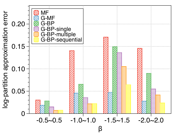
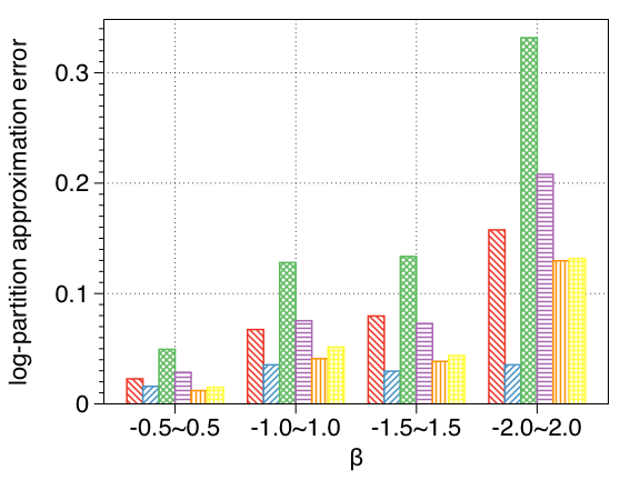
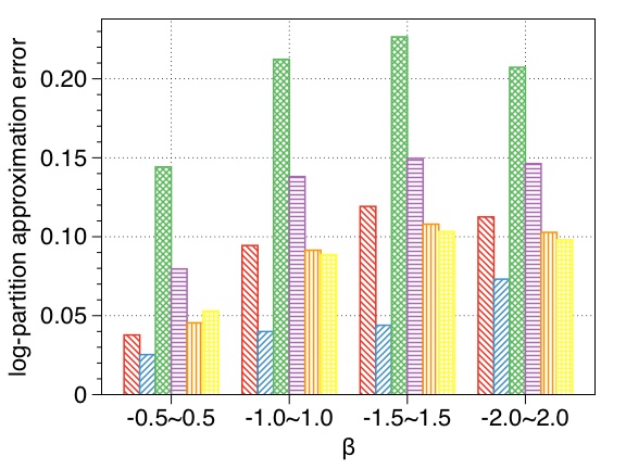
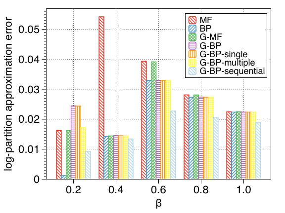
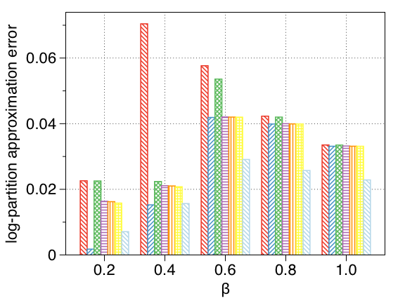
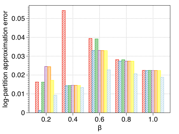
In this section, we report results of our experiments with G-MF and G-BP defined in Section 3. We also experiment here with G-BP boosted by schemes correcting errors by accounting for single (10) and multiple (11) terms, as well as correcting G-BP by applying G-BP sequentially again to each residual partition function $Z_{i}$. The error decreases, while the evaluation complexity increases, as we move from G-BP-single to G-BP-multiple and then to G-BP-sequential. As mentioned earlier, we use the IPOPT solver [33] to resolve the proposed gauge optimizations. We generate random GMs with factors dependent on the ‘interaction strength’ parameters $\{\beta_{a}\}_{a\in\mathcal{V}}$ (akin inverse temperature) as follows:

$$\mathnormal{f}_{a}(x_{a})=\exp(-\beta_{a}|h_{0}(x_{a})-h_{1}(x_{a})|),$$

where $h_{0}$ and $h_{1}$ count numbers of $0$ and $1$ contributions in $x_{a}$, respectively. Intuitively, we expect that as $|\beta_{a}|$ increases, it becomes more difficult to approximate the partition function. See the supplementary material for additional information on how we generate the random models.

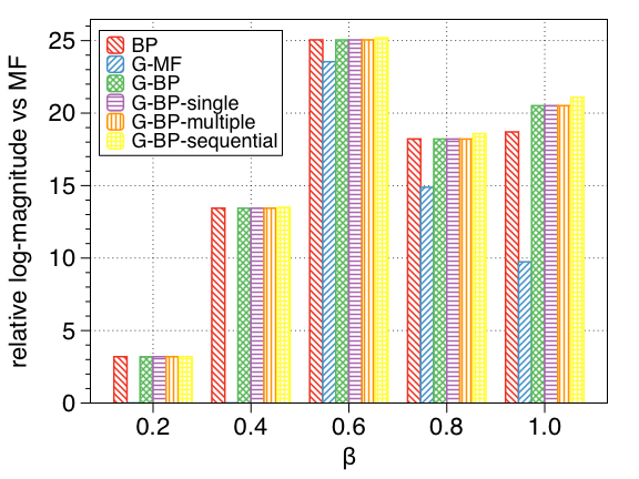
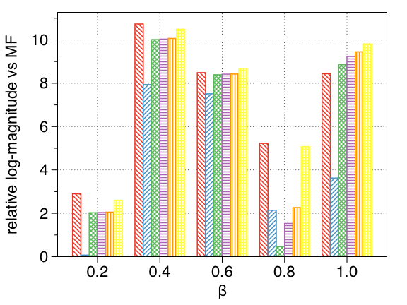
In the first set of experiments, we consider relatively small, complete graphs with two types of factors: random generic (non-log-supermodular) factors and log-supermodular (positive/ferromagnetic) factors. Recall that the bare BP also provides a lower bound in the log-supermodular case [29], thus making the comparison between each proposed algorithm and BP informative. We use the log partition approximation error defined as $|\log Z-\log Z_{\text{LB}}|/|\log Z|$, where $Z_{\text{LB}}$ is the algorithm output (a lower bound of $Z$), to quantify the algorithm’s performance. In the first set of experiments, we deal with relatively small graphs and the explicit computation of $Z$ (i.e., the approximation error) is feasible. The results for experiments over the small graphs are illustrated in Figure 1 and Figure 2 for the non-log-supermodular and log-supermodular cases, respectively. Figure 1 shows that, as expected, G-MF always outperforms MF. Moreover, we observe that G-MF typically provides the tightest low-bound, unless it is outperformed by G-BP-multiple or G-BP-sequential. We remark that BP is not shown in Figure 1, because in this non-log-supermodular case, it does not provide a lower bound in general. According to Figure 2, showing the log-supermodular case, both G-MF and G-BP outperform MF, while G-BP-sequential outperforms all other algorithms. Notice that G-BP performs rather similar to BP in the log-supermodular case, thus suggesting that the constraints, distinguishing (8) from (5), are very mildly violated.

Figure 3: Averaged ratio of the log partition function compared to MF vs graph size (i.e., number of factors) in the case of generic (non-log-supermodular) GMs on 3-regular graphs (left) and grid graphs (right), where the average is taken over 20 random models.

Figure 4: Averaged ratio of the log partition function compared to MF vs interaction strength $\beta$ in the case of log-supermodular GMs on 3-regular graphs of size 200 (left) and grid graphs of size 100 (right), where the average is taken over 20 random models.

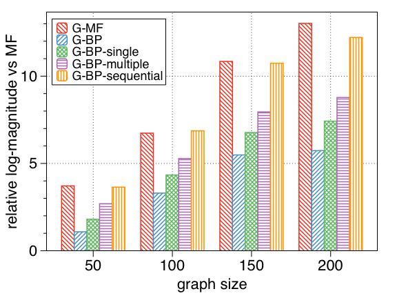
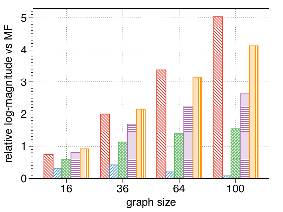
In the second set of experiments, we consider more sparse, larger graphs of two types: $3$-regular and grid graphs with size up to $200$ factors/$300$ variables. As in the first set of experiments, the same non-log-supermodular/log-supermodular factors are considered. Since computing the exact approximation error is not feasible for the large graphs, we instead measure here the ratio of estimation by the proposed algorithm to that of MF, i.e., $\log(Z_{\text{LB}}/Z_{\text{MF}})$ where $Z_{\text{MF}}$ is the output of MF. Note that a larger value of the ratio indicates better performance. The results are reported in Figure 3 and Figure 4 for the non-log-supermodular and log-supermodular cases, respectively. In Figure 3, we observe that G-MF and G-BP-sequential outperform MF significantly, e.g., up-to $e^{14}$ times better in $3$-regular graphs of size $200$. We also observe that even the bare G-BP outperforms MF. In Figure 4, algorithms associated with G-BP outperform G-MF and MF (up to $e^{25}$ times). This is because the choice of $q(x)$ for G-BP is favored by log-supermodular models, i.e., most of configurations are concentrated around $(0,0,\cdots)$ similar to the choice (7) of $q(x)$ for G-BP. One observes here (again) that performance of G-BP in this log-supermodular case is almost on par with BP. This implies that G-BP generalizes BP well: the former provides a lower bound of $Z$ for any GMs, while the latter does only for log-supermodular GMs.

5 Conclusion and future research

We explore the freedom in gauge transformations of GM and develop novel variational inference methods which result in significant improvement of the partition function estimation. In this paper, we have focused solely on designing approaches which improve the bare/basic MF and BP via specially optimized gauge transformations. In terms of the path forward, it is of interest to extend this GT framework/approach to other variational methods, e.g., Kikuchi approximation [38], structured/conditional MF [39, 40]. Furthermore, G-BP and G-MF were resolved in our experiments via a generic optimization solver (IPOPT), which was sufficient for the illustrative tests conducted so far, however we expect that it might be possible to develop more efficient distributed solvers of the BP-type. Finally, we plan working on applications of the newly designed methods and algorithms to a variety of practical inference applications associated to GMs.

Appendix A Construction of Forney-style model equivalent to factor-graph model

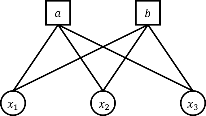
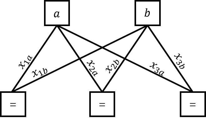
In this Section, we describe construction of a Forney-style GM equivalent to the factor-graph GM. Consider a factor-graph GM defined on graph $G=(\mathcal{X},\mathcal{F},\mathcal{E})$ with factors $\{\mathnormal{f}_{a}\}_{a\in\mathcal{F}}$. Then one introduces the following Forney-style GM defined over the graph $(\mathcal{V},\mathcal{E})$ with factors $\{\mathnormal{f}^{\dagger}_{a}\}_{a\in\mathcal{V}}$

$$\mathcal{V} \leftarrow\mathcal{X}\cup\mathcal{F},\qquad\mathnormal{f}^{\dagger}_{a}\leftarrow\mathnormal{f}_{a},\quad\forall a\in\mathcal{F},$$

$$\mathnormal{f}^{\dagger}_{a}(x_{a}) \leftarrow\begin{cases}1\quad\text{if }x_{a}=(1,1,\cdots)~{}\text{or}~{}(0,0,\cdots)\\ 0\quad\text{otherwise}\end{cases},~{}\forall a\in\mathcal{X}.$$

One observes that if the factor-graph GM (possibly, of high-order) is sparse, i.e., the maximum degree of $(\mathcal{X},\mathcal{F},\mathcal{E})$ is small, then the equivalent Forney-style GM is too. See Figure 5 for illustration.

Figure 5: Example of the transformation from the factor-graph GM (left) to the Forney-style GM (right). Factors denoted as ‘=’ constrains adjoining variables to have the same value. Originally, the factor-graph GM had $3$ variables ($x_{1},x_{2},x_{3}$) and 2 factors ($a,b$). In the equivalent Forney-style GM, there are $6$ variables ($x_{1a},x_{1b},x_{2a},x_{2b},x_{3a},x_{3b}$) and $5$ factors ($a,b$ and three ‘=’ factors).

Appendix B Proof of Theorem 1

To prove Theorem 1 one, first, shows that the line graph GM can be gauge transformed into a distribution equivalent to the alternating cycle GM. Then it is sufficient for proving Theorem 1 to consider only the case of an alternating cycle.

Consider a GM defined on a line graph $G=(\mathcal{V},\mathcal{E})$ with $\mathcal{V}=\{a_{1},a_{2},\cdots,a_{n}\}$ and edges $\mathcal{E}=\{\{a_{1},a_{2}\},\{a_{2},a_{3}\},\cdots,\{a_{n-1},a_{n}\}\}$. Then the gauge transformed factor $\mathnormal{f}_{a_{i},\mathcal{G}}$ can be expressed as:

$$\mathnormal{f}_{a_{i},\mathcal{G}}=G_{a_{i}a_{i-1}}^{\top}\mathnormal{f}_{a_{i}}G_{a_{i}a_{i+1}},$$

where we used the fact that the size/cardinality of the factor is $2$. Next, we ‘flip’ factor $\mathnormal{f}_{2}$, associated with the node number $2$, such that there exist an odd number of negative definite factors among $\mathnormal{f}_{2},\cdots\mathnormal{f}_{n-1}$, i.e., the flipping sets

$$G_{a_{1}a_{2}},G_{a_{2}a_{1}}=\left[\begin{array}[]{ccc}0&1\\ 1&0\\ \end{array}\right],$$ (12)

thus resulting in reversing the sign of $\text{det}(\mathnormal{f}_{a_{2}})$. If $\mathnormal{f}_{a_{2}}$ is non-invertible, i.e. $\text{det}(\mathnormal{f}_{a_{2}})=0$, we instead flip $\mathnormal{f}_{3}$ and so on. If all factors are non-invertible, the resulting distribution is a product distribution and one can easily find the optimal $q$ for the corresponding line graph, which completes the proof. Otherwise, we ‘join’ the endpoints $a_{1},a_{n}$ into $a_{0}$ by introducing a non-invertible factor $\mathnormal{f}_{0}=\mathnormal{f}_{1}\mathnormal{f}_{n}^{\top}$, which results in an alternating cycle with the probability distribution identical to the one of a line graph GM.

Our next step is to prove Theorem 1 for an alternating cycle GM. Our high level logic here is as follows. We first fix the distribution $q$ of (6) according to

$$\begin{split}q(x)=\begin{cases}1\qquad&\text{if }x=(0,0,\cdots),\\ 0\qquad&\text{otherwise}.\end{cases},\end{split}$$

and then show that the GM can be gauge transformed into a distribution with a nonzero probability concentrated only at $(0,0,\cdots)$. The resulting objective of (6) will become exactly the partition function. To implement this logic, consider an alternating cycle defined on some graph $G=(\mathcal{V},\mathcal{E})$ with $\mathcal{V}=\{a_{1},a_{2},\cdots,a_{n}\}$ and edges $\mathcal{E}=\{\{a_{1},a_{2}\},\{a_{2},a_{3}\},\cdots,\{a_{n-1},a_{n}\},\{a_{n},a_{1}\}\}$. Observe that, that the gauge transformed factor, $\prod_{i}\mathnormal{f}_{a_{i},\mathcal{G}}$, and the original factor, $\prod_{i}\mathnormal{f}_{a_{i}}$, share a pair of eigenvalues $\lambda_{1},\lambda_{2}$ due to the following relationship:

$$\prod_{i}\mathnormal{f}_{a_{i},\mathcal{G}}=G_{a_{n}a_{1}}^{-1}\prod_{i}\mathnormal{f}_{i}G_{a_{n}a_{1}}$$

One finds that $\lambda_{1}\lambda_{2}=\prod\text{det}(\mathnormal{f}_{i})\leq 0$ since there exist an odd number of negative definite factors in the cycle. Moreover, $\lambda_{1}+\lambda_{2}>0$ because the diagonal sum, $\prod_{i}\mathnormal{f}_{i}$, is equivalent to the partition function of GM. Thus one can assume, without loss of generality, that $\lambda_{1}>0$ and $\lambda_{2}<0$.

Next, utilizing a simple linear algebra, one derives

$$Q_{2}^{-1}Q_{1}G_{a_{n}a_{1}}\prod_{i}\mathnormal{f}_{i,\mathcal{G}}Q^{-1}_{1}Q_{2}=\left[\begin{array}[]{ccc}\lambda_{1}+\lambda_{2}&\lambda_{1}\\ -\lambda_{2}&0\\ \end{array}\right],$$

where $Q_{1}$ and $Q_{2}$ are matrices whose $j$-th column is an eigen-vector of $\prod_{i}\mathnormal{f}_{i}$ and, $\left[\begin{array}[]{ccc}\lambda_{1}+\lambda_{2}&\lambda_{1}\\ -\lambda_{2}&0\\ \end{array}\right]$, respectively. Now let

$$G_{a_{n}a_{1}}=Q_{1}^{-1}Q_{2},\qquad G_{a_{i-1}a_{i}}=(\mathnormal{f}_{i}G_{a_{i}a_{i+1}}^{\top})^{-1}\quad\text{for}\quad i=2,\cdots n,$$

where $a_{n+1}=a_{1}$. Here we assume that there exists at most one non-invertible factor in the GM and $\mathnormal{f}_{2},\cdots,\mathnormal{f}_{n}$ are invertible so that $(\mathnormal{f}_{i}G_{a_{i}a_{i+1}}^{\top})^{-1}$ is defined properly. Otherwise, the GM can be decomposed into separate line graphs and the proof can be applied recursively. Then the gauge transformed factors become:

$$\mathnormal{f}_{a_{1},\mathcal{G}}=\left[\begin{array}[]{ccc}\lambda_{1}+\lambda_{2}&\lambda_{1}\\ -\lambda_{2}&0\\ \end{array}\right],\quad\mathnormal{f}_{a_{i},\mathcal{G}}=\left[\begin{array}[]{ccc}1&0\\ 0&1\\ \end{array}\right]\quad\forall i\neq 1,$$

which corresponds to a GM with objective of (6) to be equal to the log partition function. This completes the proof of the Theorem 1.

Appendix C Generating GM instances (for experiments)

In this Section, we provide more details on our experimental setups reported in in Section 4. First, we explain how the two types of factors, non-log-supermodular and log-supermodular, were constructed. In the generic case (of non-log-supermodular factors), i.e., correspondent to Figure 1 and Figure 3, one generates factor by first drawing the interaction strength vector at random from the i.i.d. uniform distribution over the interval $[-T,T]$ for some $T>0$, i.e., $\beta_{a}\sim\mathcal{U}(-T,T)$. Then, in order to introduce a bias, we add an external variable $y_{a}$, i.e., half-edge, as follows:

$$\mathnormal{f}_{a}(x_{a})=\exp(\beta_{a}|h_{0}(x_{a}\cup y_{a})-h_{1}(x_{a}\cup y_{a})|),$$

where $y_{a}$ is either $\{0\}$ or $\{1\}$ with probability $1/2$ each. More specifically in experiments resulted in Figure 1 one varies $T$ while in the experiments resulted in Figure 3 one fixes $T$ to $1.0$, i.e., $\beta_{a}\sim[-1.0,1.0]$. Next, in the case of the log-supermodular factors, i.e., setting resulted in Figure 2 and Figure 4, one generates log-supermodular factors by drawing the interaction strength vector from normal distribution with the average $T>0$ and the variance, $10^{-4}$, i.e., $\beta_{a}\sim\mathcal{N}(T,10^{-4})$. Note that there exist no bias in the factors and even though the distribution of the interaction strength is normal, it is highly likely to observe a positive value concentrated around $T$.

References

- [1] Robert Gallager. Low-density parity-check codes. IRE Transactions on information theory, 8(1):21–28, 1962.
- [2] Frank R. Kschischang and Brendan J. Frey. Iterative decoding of compound codes by probability propagation in graphical models. IEEE Journal on Selected Areas in Communications, 16(2):219–230, 1998.
- [3] Hans .A. Bethe. Statistical theory of superlattices. Proceedings of Royal Society of London A, 150:552, 1935.
- [4] Rudolf E. Peierls. Ising’s model of ferromagnetism. Proceedings of Cambridge Philosophical Society, 32:477–481, 1936.
- [5] Marc Mézard, Georgio Parisi, and M. A. Virasoro. Spin Glass Theory and Beyond. Singapore: World Scientific, 1987.
- [6] Giorgio Parisi. Statistical field theory, 1988.
- [7] Marc Mezard and Andrea Montanari. Information, Physics, and Computation. Oxford University Press, Inc., New York, NY, USA, 2009.
- [8] Judea Pearl. Probabilistic reasoning in intelligent systems: networks of plausible inference. Morgan Kaufmann, 2014.
- [9] Michael Irwin Jordan. Learning in graphical models, volume 89. Springer Science & Business Media, 1998.
- [10] William T Freeman, Egon C Pasztor, and Owen T Carmichael. Learning low-level vision. International journal of computer vision, 40(1):25–47, 2000.
- [11] Mark Jerrum and Alistair Sinclair. Polynomial-time approximation algorithms for the ising model. SIAM Journal on computing, 22(5):1087–1116, 1993.
- [12] Ethem Alpaydin. Introduction to machine learning. MIT press, 2014.
- [13] Judea Pearl. Reverend Bayes on inference engines: A distributed hierarchical approach. Cognitive Systems Laboratory, School of Engineering and Applied Science, University of California, Los Angeles, 1982.
- [14] Qiang Liu and Alexander T Ihler. Negative tree reweighted belief propagation. arXiv preprint arXiv:1203.3494, 2012.
- [15] Stefano Ermon, Ashish Sabharwal, Bart Selman, and Carla P Gomes. Density propagation and improved bounds on the partition function. In Advances in Neural Information Processing Systems, pages 2762–2770, 2012.
- [16] Martin J Wainwright, Tommi S Jaakkola, and Alan S Willsky. A new class of upper bounds on the log partition function. IEEE Transactions on Information Theory, 51(7):2313–2335, 2005.
- [17] Qiang Liu and Alexander T Ihler. Bounding the partition function using holder’s inequality. In Proceedings of the 28th International Conference on Machine Learning (ICML-11), pages 849–856, 2011.
- [18] Martin J. Wainwright, Tommy S. Jaakkola, and Alan S. Willsky. Tree-based reparametrization framework for approximate estimation on graphs with cycles. Information Theory, IEEE Transactions on, 49(5):1120–1146, 2003.
- [19] Michael Chertkov and Vladimir Chernyak. Loop calculus in statistical physics and information science. Physical Review E, 73:065102(R), 2006.
- [20] Michael Chertkov and Vladimir Chernyak. Loop series for discrete statistical models on graphs. Journal of Statistical Mechanics, page P06009, 2006.
- [21] Leslie G Valiant. Holographic algorithms. SIAM Journal on Computing, 37(5):1565–1594, 2008.
- [22] Ali Al-Bashabsheh and Yongyi Mao. Normal factor graphs and holographic transformations. IEEE Transactions on Information Theory, 57(2):752–763, 2011.
- [23] Martin J. Wainwright and Michael E. Jordan. Graphical models, exponential families, and variational inference. Foundations and Trends in Machine Learning, 1(1):1–305, 2008.
- [24] G David Forney Jr and Pascal O Vontobel. Partition functions of normal factor graphs. arXiv preprint arXiv:1102.0316, 2011.
- [25] Michael Chertkov. Lecture notes on “statistical inference in structured graphical models: Gauge transformations, belief propagation & beyond", 2016.
- [26] J. S. Yedidia, W. T. Freeman, and Y. Weiss. Constructing free-energy approximations and generalized belief propagation algorithms. Information Theory, IEEE Transactions on, 51(7):2282–2312, 2005.
- [27] Vladimir Y Chernyak and Michael Chertkov. Loop calculus and belief propagation for q-ary alphabet: Loop tower. In Information Theory, 2007. ISIT 2007. IEEE International Symposium on, pages 316–320. IEEE, 2007.
- [28] Ryuhei Mori. Holographic transformation, belief propagation and loop calculus for generalized probabilistic theories. In Information Theory (ISIT), 2015 IEEE International Symposium on, pages 1099–1103. IEEE, 2015.
- [29] Nicholas Ruozzi. The bethe partition function of log-supermodular graphical models. In Advances in Neural Information Processing Systems, pages 117–125, 2012.
- [30] Adrian Weller, Kui Tang, Tony Jebara, and David Sontag. Understanding the bethe approximation: when and how can it go wrong? In UAI, pages 868–877, 2014.
- [31] Michael Chertkov, Vladimir Y Chernyak, and Razvan Teodorescu. Belief propagation and loop series on planar graphs. Journal of Statistical Mechanics: Theory and Experiment, 2008(05):P05003, 2008.
- [32] Sung-Soo Ahn, Michael Chertkov, and Jinwoo Shin. Synthesis of mcmc and belief propagation. In Advances in Neural Information Processing Systems, pages 1453–1461, 2016.
- [33] Andreas Wächter and Lorenz T Biegler. On the implementation of an interior-point filter line-search algorithm for large-scale nonlinear programming. Mathematical programming, 106(1):25–57, 2006.
- [34] G David Forney. Codes on graphs: Normal realizations. IEEE Transactions on Information Theory, 47(2):520–548, 2001.
- [35] Martin Wainwright and Michael Jordan. Graphical models, exponential families, and variational inference. Technical Report 649, UC Berkeley, Department of Statistics, 2003.
- [36] Jonathan S Yedidia, William T Freeman, and Yair Weiss. Bethe free energy, kikuchi approximations, and belief propagation algorithms. Advances in neural information processing systems, 13, 2001.
- [37] Michael Chertkov and Vladimir Y Chernyak. Loop series for discrete statistical models on graphs. Journal of Statistical Mechanics: Theory and Experiment, 2006(06):P06009, 2006.
- [38] Ryoichi Kikuchi. A theory of cooperative phenomena. Physical review, 81(6):988, 1951.
- [39] Lawrence K Saul and Michael I Jordan. Exploiting tractable substructures in intractable networks. Advances in neural information processing systems, pages 486–492, 1996.
- [40] Peter Carbonetto and Nando D Freitas. Conditional mean field. In Advances in neural information processing systems, pages 201–208, 2007.