When Hashes Met Wedges: A Distributed Algorithm for Finding High Similarity Vectors

Abstract

Finding similar user pairs is a fundamental task in social networks, with numerous applications in ranking and personalization tasks such as link prediction and tie strength detection. A common manifestation of user similarity is based upon network structure: each user is represented by a vector that represents the user’s network connections, where pairwise cosine similarity among these vectors defines user similarity. The predominant task for user similarity applications is to discover all similar pairs that have a pairwise cosine similarity value larger than a given threshold $\tau$. In contrast to previous work where $\tau$ is assumed to be quite close to 1, we focus on recommendation applications where $\tau$ is small, but still meaningful. The all pairs cosine similarity problem is computationally challenging on networks with billions of edges, and especially so for settings with small $\tau$. To the best of our knowledge, there is no practical solution for computing all user pairs with, say $\tau=0.2$ on large social networks, even using the power of distributed algorithms.

Our work directly addresses this challenge by introducing a new algorithm — WHIMP — that solves this problem efficiently in the MapReduce model. The key insight in WHIMP is to combine the “wedge-sampling" approach of Cohen-Lewis for approximate matrix multiplication with the SimHash random projection techniques of Charikar. We provide a theoretical analysis of WHIMP, proving that it has near optimal communication costs while maintaining computation cost comparable with the state of the art. We also empirically demonstrate WHIMP’s scalability by computing all highly similar pairs on four massive data sets, and show that it accurately finds high similarity pairs. In particular, we note that WHIMP successfully processes the entire Twitter network, which has tens of billions of edges.

1 Introduction

Similarity search among a collection of objects is one of the oldest and most fundamental operations in social networks, web mining, data analysis and machine learning. It is hard to overstate the importance of this problem: it is a basic building block of personalization and recommendation systems [12, 21], link prediction [1, 30], and is found to be immensely useful in many personalization and mining tasks on social networks and databases [41, 33, 42, 35]. Indeed, the list of applications is so broad that we do not attempt to survey them here and instead refer to recommender systems and data mining textbooks that cover applications in diverse areas such as collaborative filtering [35, 29].

Given the vast amount of literature on similarity search, many forms of the problem have been studied in various applications. In this work we focus on the social and information networks setting where we can define pairwise similarity among users on the network based on having common connections. This definition of similarity is particularly relevant in the context of information networks where users generate and consume content (Twitter, blogging networks, web networks, etc.). In particular, the directionality of these information networks provides a natural measure that is sometimes called “production” similarity: two users are defined to be similar to each other if they are followed by a common set of users. Thus, “closeness" is based on common followers, indicating that users who consume content from one of these users may be interested in the other “producer” as well. The most common measure of closeness or similarity here is cosine similarity. This notion of cosine similarity is widely used for applications [1, 26, 5, 30] and is in particular a fundamental component of the Who To Follow recommendation system at Twitter [20, 21].

Our focus in this work is on the computational aspect of this widely important and well studied problem. In particular, despite the large amount of attention given to the problem, there remain significant scalability challenges with computing all-pairs similarity on massive size information networks. A unique aspect of this problem on these large networks is that cosine similarity values that are traditionally considered “small” can be quite meaningful for social and information network applications — it may be quite useful and indicative to find users sharing a cosine similarity value of 0.2, as we will illustrate in our experimental results. With this particular note in mind, we move on to describing our problem formally and discuss the challenges involved in solving it at scale.

(a)

(b)

(c)

Figure 1: Result on WHIMP for $\tau=0.2$: the left plot the precision-recall curves for finding all entries in $A^{T}A$ above $0.2$ (with respect to a sampled evaluation set). The other plots give the cumulative distribution, over all sampled users, of the minimum of precision and recall. We observe that for an overwhelming majority of users, WHIMP reliably finds more than 70% of $0.2$-similar users.

1.1 Problem Statement

As mentioned earlier, the similarity search problem is relevant to a wide variety of areas, and hence there are several languages for describing similarity: on sets, on a graph, and also on matrix columns. We’ll attempt to provide the different views where possible, but we largely stick to the matrix notation in our work. Given two sets $S$ and $T$, their cosine similarity is $|S\cap T|/\sqrt{|S|\cdot|T|}$, which is a normalized intersection size. It is instructive to define this geometrically, by representing a set as an incidence vector. Given two (typically non-negative) vectors $\vec{v}_{1}$ and $\vec{v}_{2}$, the cosine similarity is $\vec{v}_{1}\cdot\vec{v}_{2}/(\|\vec{v}_{1}\|_{2}\|\vec{v}_{2}\|_{2})$. This is the cosine of the angle between the vectors; hence the name.

In our context, the corresponding $\vec{v}$ for some user is the incidence vector of followers. In other words, the $i$th coordinate of $\vec{v}$ is $1$ if user $i$ follows the user, and $0$ otherwise. Abusing notation, let us denote the users by their corresponding vectors, and we use the terms “user" and “vector" interchangably. Thus, we can define our problem as follows.

Problem 1.1

Given a sets of vectors $\vec{v}_{1},\vec{v}_{2},\ldots,\vec{v}_{m}$ in $(\mathbb{R}^{+})^{d}$, and threshold $\tau>0$: determine all pairs $(i,j)$ such that $\vec{v}_{i}\cdot\vec{v}_{j}\geq\tau$.

Equivalently, call $\vec{v}_{j}$ $\tau$-similar to $\vec{v}_{i}$ if $\vec{v}_{i}\cdot\vec{v}_{j}\geq\tau$. For every vector $\vec{v}_{i}$, find all vectors $\tau$-similar to $\vec{v}_{j}$.

In terms of (approximate) information retrieval, the latter formulation represents a more stringent criterion. Instead of good accuracy in find similar pairs overall, we demand high accuracy for most (if not all) users. This is crucial for any recommendation system, since we need good results for most users. More generally, we want good results at all “scales", meaning accurate results for users with small followings as well as big followings. Observe that the sparsity of $\vec{v}$ is inversely related to the indegree (following size) of the user, and represents their popularity. Recommendation needs to be of high quality both for newer users (high sparsity $\vec{v}$) and celebrities (low sparsity $\vec{v}$).

We can mathematically express Problem 1.1 in matrix terms as follows. Let $A$ be the $d\times n$ matrix where the $i$th column is $\vec{v}_{i}/\|\vec{v}_{i}\|_{2}$. We wish to find all large entries in the Gramian matrix $A^{T}A$ (the matrix of all similarities). It is convenient to think of the input as $A$. Note that the non-zeros of $A$ correspond exactly to the underlying social network edges.

1.2 Challenges

Scale: The most obvious challenge for practical applications is the sheer size of the matrix $A$. For example, the Twitter recommendation systems deal with a matrix with hundreds of millions of dimensions, and the number of non-zeros is in many tens of billions. Partitioning techniques become extremely challenging for these sizes and clearly we need distributed algorithms for Problem 1.1.

The similarity value $\tau$: An equally important (but less discussed) problem is the relevant setting of threshold $\tau$ in Problem 1.1. In large similarity search applications, a cosine similarity (between users) of, say, $0.2$ is highly significant. Roughly speaking, if user $u$ is $0.2$-similar to $v$, then 20% of $u$’s followers also follow $v$. For recommendation, this is an immensely strong signal. But for many similarity techniques based on hashing/projection, this is too small [24, 3, 37, 39, 38, 4]. Techniques based on LSH and projection usually detect similarities above 0.8 or higher. Mathematically, these methods have storage complexities that scale as $1/\tau^{2}$, and are simply infeasible when $\tau$ is (say) $0.2$.

We stress that this point does not receive much attention. But in our view, it is the primary bottleneck behind the lack of methods to solve Problem 1.1 for many real applications.

The practical challenge: This leads us to main impetus behind our work.

For the matrix $A$ corresponding to the Twitter network with $O(100\textrm{B})$ edges, find (as many as possible) entries in $A^{T}A$ above $0.2$. For a majority of users, reliably find many $0.2$-similar users.

1.3 Why previous approaches fail

The challenge described above exemplifies where big data forces an algorithmic rethink. Matrix multiplication and variants thereof have been well-studied in the literature, but no solution works for such a large matrix. If a matrix $A$ has a 100 billion non-zeroes, it takes upwards of 1TB just to store the entries. This is more than an order of magnitude of the storage of a commodity machine in a cluster. Any approach of partitioning $A$ into submatrices cannot scale.

There are highly tuned libraries like Intel MKL’s BLAS [25] and CSparse [13]. But any sparse matrix multiplication routine [22, 2] will generate all triples $(i,i^{\prime},j)$ such that $A_{i,j}A_{i^{\prime},j}\neq 0$. In our example, this turns out to be more than 100 trillion triples. This is infeasible even for a large industrial-strength cluster.

Starting from the work of Drineas, Kannan, and Mahoney, there is rich line of results on approximate matrix multiplication by subsampling rows of the matrix [15, 17, 16, 36, 7, 32, 34, 23]. These methods generate approximate products according to Frobenius norm using outer products of columns. This would result in dense matrices, which is clearly infeasible at our scale. In any case, the large entries (of interest) contribute to a small part of the output.

Why communication matters: There are upper bounds on the total communication even in industrial-strength Hadoop clusters, and in this work we consider our upper bound to be about 100TB. A promising approach for Problem 1.1 is the wedge sampling method of Cohen-Lewis [11], which was further developed in the diamond sampling work of Ballard et al [6]. The idea is to set up a linear-sized data structure that can sample indices of entries proportional to value (or values squared in [6]). One then generates many samples, and picks the index pairs that occur most frequently. These samples can be generated in a distributed manner, as shown by Zadeh and Goel [43].

The problem is in the final communication. The sampling calculations show that about $10\tau^{-1}\sum_{i,j}\vec{a_{i}}\cdot\vec{a_{j}}$ samples are required to get all entries above $\tau$ with high probability. These samples must be collected/shuffled to actually find the large entries. In our setting, this is upwards of 1000TB of communication.

Locality Sensitive Hashing: In the normalized setting, maximizing dot product is equivalent to minimizing distance. Thus, Problem 1.1 can be cast in terms of finding all pairs of points within some distance threshold. A powerful technique for this problem is Locality Sensitive Hashing (LSH) [24, 18, 3]. Recent results by Shrivastava and Li use LSH ideas for the MIPS problem [37, 39, 38]. This essentially involves carefully chosen low dimensional projections with a reverse index for fast lookup. It is well-known that LSH requires building hashes that are a few orders of magnitude more than the data size. Furthermore, in our setting, we need to make hundreds of millions of queries, which involve constructing all the hashes, and shuffling them to find the near neighbors. Again, this hits the communication bottleneck.

1.4 Results

We design WHIMP, a distributed algorithm to solve Problem 1.1. We specifically describe and implement WHIMP in the MapReduce model, since it is the most appropriate for our applications.

Theoretical analysis: WHIMP is a novel combination of wedge sampling ideas from Cohen-Lewis [11] with random projection-based hashes first described by Charikar [10]. We give a detailed theoretical analysis of WHIMP and prove that it has near optimal communication/shuffle cost, with a computation cost comparable to the state-of-the-art. To the best of our knowledge, it is the first algorithm to have such strong guarentees on the communication cost. WHIMP has a provable precision and recall guarantee, in that it outputs all large entries, and does not output small entries.

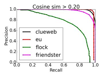
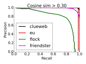
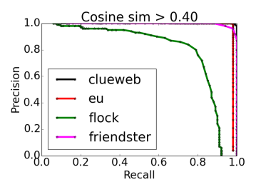
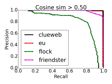
Empirical demonstration: We implement WHIMP on Hadoop and test it on a collection of large networks. Our largest network is flock, the Twitter network with tens of billions of non-zeroes. We present results in Fig. 1. For evaluation, we compute ground truth for a stratified sample of users (details in §7). All empirical results are with respect to this evaluation. Observe the high quality of precision and recall for $\tau=0.2$. For all instances other than flock (all have non-zeros between 1B to 100B), the accuracy is near perfect. For flock, WHIMP dominates a precision-recall over $(0.7,0.7)$, a significant advance for Problem 1.1 at this scale.

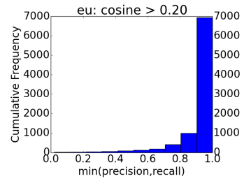
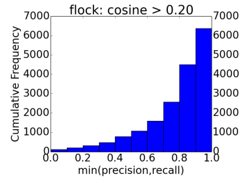
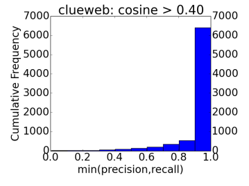
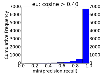
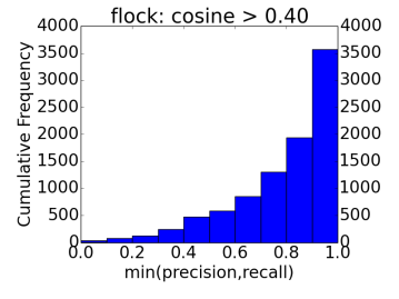
Even more impressive are the distribution of precision-recall values. For each user in the evaluation sample (and for a specific setting of parameters in WHIMP), we compute the precision and recall $0.2$-similar vectors. We plot the cumulative histogram of the minimum of the precision and recall (a lower bound on any F-score) for two of the largest datasets, eu (a web network) and flock. For more than 75% of the users, we get a precision and recall of more than $0.7$ (for eu, the results are even better). Thus, we are able to meet our challenge of getting accurate results on an overwhelming majority of users. (We note that in recent advances in using hashing techniques [37, 39, 38], precision-recall curves rarely dominate the point $(0.4,0.4)$.)

2 Problem Formulation

Recall that the problem of finding similar users is a special case of Problem 1.1. Since our results extend to the more general setting, in our presentation we focus on the $A^{T}B$ formulation for given matrices $A$ and $B$. The set of columns of $A$ is the index set $[m]$, denoted by $C_{A}$. Similarly, the set of columns of $B$, indexed by $[n]$, is denoted by $C_{B}$. The dimensions of the underlying space are indexed by $D=[d]$. We use $a_{1},\ldots$ to denote columns of $A$, $b_{1},\ldots$ for columns in $B$, and $r_{1},r_{2},\ldots$ for dimensions. For convenience, we assume wlog that $n\geq m$.

We denote rows and columns of $A$ by $A_{d,*}$ and $A_{*,a}$ respectively. And similar notation is used for $B$. We also use $\mathrm{nnz}(\cdot)$ to denote the number of non-zeroes in a matrix. For any matrix $M$ and $\sigma\in\mathbb{R}$, the thresholded matrix $[M]_{\geq\sigma}$ keeps all values in $M$ that are at least $\sigma$. In other words, $([M]_{\geq\sigma})_{i,j}=M_{i,j}$ if $M_{i,j}\geq\sigma$ and zero otherwise. We use $\|M\|_{1}$ to be the entrywise 1-norm. We will assume that $\|A^{T}B\|_{1}\geq 1$. This is a minor technical assumption, and one that always holds in matrix products of interest.

We can naturally represent $A$ as a (weighted) bipartite graph $G_{A}=(C_{A},D,E_{A})$, where an edge $(a,d)$ is present iff $A_{d,a}\neq 0$. Analogously, we can define the bipartite graph $G_{B}$. Their union $G_{A}\cup G_{B}$ is a tripartite graph denoted by $G_{A,B}$. For any vertex $v$ in $G_{A,B}$, we use $N(v)$ for the neighborhood of $v$.

Finally, we will assume the existence of a Gaussian random number generator $g$. Given a binary string $x$ as input, $g(x)\sim{\cal N}(0,1)$. We assume that all values of $g$ are independent.

The computational model: While our implementation (and focus) is on MapReduce, it is convenient to think of an abstract distributed computational model that is also a close proxy for MapReduce in our setting [19]. This allows for a transparent explanation of the computation and communication cost.

Let each vertex in $G_{A,B}$ be associated with a different processor. Communication only occurs along edges of $G_{A,B}$, and occurs synchronously. Each round of communication involves a single communication over all edges of $G_{A,B}$.

3 High Level Description

The starting point of our WHIMP algorithm (Wedges and Hashes in Matrix Product) is the wedge sampling method of Cohen-Lewis. A distributed MapReduce implementation of wedge sampling (for the special case of $A=B$) was given by Zadeh-Goel [43]. In effect, the main distributed step in wedge sampling is the following. For each dimension $r\in[d]$ (independently and in parallel), we construct two distributions on the index sets of vectors in $A$ and $B$. We then choose a set of independent samples for each of these distributions, to get pairs $(a,b)$, where $a$ indexes a vector in $A$, and $b$ indexes a vector in $B$. These are the “candidates" for high similarity. If enough candidates are generated, we are guaranteed that the candidates that occur with high enough frequency are exactly the large entries of $A^{T}B$.

The primary bottleneck with this approach is that the vast majority of pairs generated occur infrequently, but dominate the total shuffle cost. In particular, most non-zero entries in $A^{T}B$ are very small, but in total, these entries account for most of $\|A^{T}B\|_{1}$. Thus, these low similarity value pairs dominate the output of wedge sampling.

Our main idea is to construct an efficient, local “approximate oracle" for deciding if $A_{*,a}\cdot B_{*,b}\geq\tau$. This is achieved by adapting the well-known SimHash projection scheme of Charikar [10]. For every vector $\vec{v}$ in our input, we construct a compact logarithmic sized hash $h(\vec{v})$. By the properties of SimHash, it is (approximately) possible to determine if $\vec{u}\cdot\vec{v}\geq\tau$ only given the hashes $h(\vec{u})$ and $h(\vec{v})$. These hashes can be constructed by random projections using near-linear communication. Now, each machine that processes dimension $r$ (of the wedge sampling algorithm) collects every hash $h(A_{*,a})$ for each $a$ such that $A_{r,a}\neq 0$ (similarly for $B$). This adds an extra near-linear communication step, but all these hashes can now be stored locally in the machine computing wedge samples for dimension $r$. This machines runs the same wedge sampling procedure as before, but now when it generates a candidate $(a,b)$, it first checks if $A_{*,a}\cdot B_{*,b}\geq\tau$ using the SimHash oracle. And this pair is emitted iff this condition passes. Thus, the communication of this step is just the desired output, since very few low similarity pairs are emitted. The total CPU/computation cost remains the same as the Cohen-Lewis algorithm.

4 The significance of the main theorem

Before describing the actual algorithm, we state the main theorem and briefly describe its significance.

Theorem 4.1

Given input matrices $A,B$ and threshold $\tau$, denote the set of index pairs output by WHIMP algorithm by $S$. Then, fixing parameters $\ell=\lceil c\tau^{-2}\log n\rceil$, $s=(c(\log n)/\tau)$, and $\sigma=\tau/2$ for a sufficiently large constant $c$, the WHIMP algorithm has the following properties with probability at least $1-1/n^{2}$:

• [Recall:] If $(A^{T}B)_{a,b}\geq\tau$, $(a,b)$ is output.

• [Precision:] If $(a,b)$ is output, $(A^{T}B)_{a,b}\geq\tau/4$.

• The total computation cost is $O(\tau^{-1}\|A^{T}B\|_{1}\log n$ $+\tau^{-2}$ $(\mathrm{nnz}(A)$ $+\mathrm{nnz}(B))\log n)$.

• The total communication cost is $O((\tau^{-1}\log n)\|[A^{T}B]_{\geq\tau/4}\|_{1}$ $+\mathrm{nnz}(A)+\mathrm{nnz}(B)+\tau^{-2}(m+n)\log n)$.

As labeled above, the first two items above are recall and precision. The first term in the total computation cost is exactly that of vanilla wedge sampling, $\tau^{-1}\|A^{T}B\|_{1}\log n$, while the second is an extra near-linear term. The total communication of wedge sampling is also $\tau^{-1}\|A^{T}B\|_{1}\log n$. Note that WHIMP has a communication of
$\tau^{-1}\|[A^{T}B]_{\geq\tau/4}\|_{1}\log n$. Since all entries in $A^{T}B$ are at most $1$, $\|[A^{T}B]_{\geq\tau/4}\|_{1}\leq\mathrm{nnz}([A^{T}B]_{\geq\tau/4})$. Thus, the communication of WHIMP is at most $(\tau^{-1}\log n)\mathrm{nnz}([A^{T}B]_{\geq\tau/4}$ plus an additional linear term. The former is (up to the $\tau^{-1}\log n$ term) simply the size of the output, and must be paid by any algorithm that outputs all entries above $\tau/4$. Finally, we emphasize that the constant of $4$ is merely a matter of convenience, and can be replaced with any constant $(1+\delta)$.

In summary, Theorem 4.1 asserts that WHIMP has (barring additional near-linear terms) the same computation cost as wedge sampling, with nearly optimal communication cost.

5 The WHIMP algorithm

The WHIMP algorithm goes through three rounds of communication, each of which are described in detail in Figure 2. The output of WHIMP is a list of triples $((a,b),\mathrm{est}_{a,b})$, where $\mathrm{est}_{a,b}$ is an estimate for $(A^{T}B)_{a,b}$. Abusing notation, we say a pair $(a,b)$ is output, if it is part of some triple that is output.

In each round, we have a step “Gather". The last round has an output operation. These are the communication operation. All other steps are compute operations that are local to the processor involved.

WHIMP Round 1 (Hash Computation): 1. For each $a\in C_{A}$: (a) Gather column $A_{*,a}$. (b) Compute $\|A_{*,a}\|_{2}$. (c) Compute bit array $h_{a}$ of length $\ell$ as follows: $h_{a}[i]=\mathrm{sgn}\left(\sum_{r\in[d]}g(\langle r,i\rangle)A_{r,a}\right)$. 2. Perform all the above operations for all $b\in C_{B}$. WHIMP Round 2 (Weight Computation): 1. For all $r\in[d]$: (a) Gather rows $A_{r,*}$ and $B_{r,*}$. (b) Compute $\|A_{r,*}\|_{1}$ and construct a data structure that samples $a\in C_{A}$ proportional to $A_{r,a}/\|A_{r,*}\|_{1}$. Call this distribution ${\cal A}_{r}$. (c) Similarly compute $\|B_{r,*}\|_{1}$ and sampling data structure for $\mathcal{B}_{r}$. WHIMP Round 3 (Candidate Generation): 1. For all $r\in[d]$: (a) Gather: For all $a,b\in N(r)$, $h_{a},h_{b},\|A_{*,a}\|_{2},\|B_{*,b}\|_{2}$. (b) Repeat $s\|A_{r,*}\|_{1}\|B_{r,*}\|_{1}/$ ($s$ set to $c(\log n)/\tau$) times: i. Generate $a\sim{\cal A}_{r}$. ii. Generate $b\sim\mathcal{B}_{r}$. iii. Denote the Hamming distance between bit arrays $h_{a}$ and $h_{b}$ by $\Delta$. iv. Compute $\mathrm{est}_{a,b}=\|A_{*,a}\|_{2}\|B_{*,b}\|_{2}\cos(\pi\Delta/\ell)$. v. If $\mathrm{est}\geq\sigma$, emit $((a,b),\mathrm{est}_{a,b})$.

Figure 2: The WHIMP (Wedges And Hashes In Matrix Product) algorithm

Lemma 5.1

With probability at least $1-1/n^{6}$ over the randomness of WHIMP, for all pairs $(a,b)$, $|\mathrm{est}_{a,b}-A_{*,a}\cdot B_{*,b}|\leq\tau/4$.

Proof 5.2.

First fix a pair $(a,b)$. We have $\mathrm{est}_{a,b}=\|A_{*,a}\|_{2}\|B_{*,b}\|_{2}$ $\cos(\pi\Delta/\ell)$, where $\Delta$ is the Hamming distance between $h_{a}$ and $h_{b}$. Note that $h_{a}[i]=\mathrm{sgn}(\sum_{r\in[d]}g(\langle r,i\rangle)A_{r,a})$. Let $\vec{v}$ be the $d$-dimension unit vector with $r$th entry proportional to $g(\langle r,i\rangle)$. Thus, the $r$th component is a random (scaled) Gaussian, and $\vec{v}$ is a uniform (Gaussian) random vector in the unit sphere. We can write $h_{a}[i]=\mathrm{sgn}(\vec{v}\cdot A_{*,a})$ and $h_{b}[i]=\mathrm{sgn}(\vec{v}\cdot B_{*,b})$. The probability that $h_{a}[i]\neq h_{b}[i]$ is exactly the probability that the vectors $A_{*,a}$ and $B_{*,b}$ are on different sides of a randomly chosen hyperplane. By a standard geometric argument [10], if $\theta_{a,b}$ is the angle between the vectors $A_{*,a}$ and $B_{*,b}$, then this probability is $\theta_{a,b}/\pi$.

Define $X_{i}$ to be the indicator random variable for $h_{a}[i]\neq h_{b}[i]$. Note that the Hamming distance $\Delta=\sum_{i\leq\ell}X_{i}$ and $\hbox{\bf E}[\Delta]=\ell\theta_{a,b}/\pi$. Applying Hoeffding’s inequality,

$$\Pr[|\Delta-\hbox{\bf E}[\Delta]|\geq\ell\tau/(4\pi\|A_{*,a}\|_{2}\|B_{*,b}\|_{2})]$$

$$< \exp[-(\ell^{2}\tau^{2}/16\pi^{2}\|A_{*,a}\|^{2}_{2}\|B_{*,b}\|^{2}_{2})/2\ell]$$

$$= \exp(-(c/\tau^{2})(\log n)\tau^{2}/(32\pi^{2}\|A_{*,a}\|^{2}_{2}\|B_{*,b}\|^{2}_{2}))<n^{-8}$$

Thus, with probability $>1-n^{-8}$,
$|\pi\Delta/\ell-\theta_{a,b}|\leq$ $\tau/(4\|A_{*,a}\|_{2}\|B_{*,b}\|_{2})$. By the Mean Value Theorem, $|\cos(\pi\Delta/\ell)-\cos(\theta_{a,b})|\leq\tau/(4\|A_{*,a}\|_{2}\|B_{*,b}\|_{2})$. Multiplying by $\|A_{*,a}\|_{2}\|B_{*,b}\|_{2}$, we get $|\mathrm{est}_{a,b}-A_{*,a}\cdot B_{*,b}|\leq\tau/4$. We take a union bound over all $\Theta(mn)$ pairs $(a,b)$ to complete the proof.

We denote a pair $(a,b)$ as generated if it is generated in Steps 1(b)i and 1(b)ii during some iteration. Note that such a pair is actually output iff $\mathrm{est}_{a,b}$ is sufficiently large.

Lemma 5.3.

With probability at least $1-1/n^{3}$ over the randomness of WHIMP, the following hold. The total number of triples output is $O((\tau^{-1}\log n)\max(\|[A^{T}_{B}]_{\geq\tau/4}\|_{1},1))$. Furthermore, if $A_{*,a}\cdot B_{*,b}\geq\tau$, $(a,b)$ is output.

Proof 5.4.

Let $X_{a,b,r,i}$ be the indicator random variable for $(a,b)$ being output in the $i$ iteration for dimension $r$. The total number of times that $(a,b)$ is output is exactly $X_{a,b}=\sum_{r,i}X_{a,b,r,i}$. By the definition of the distributions ${\cal A}_{r}$ and $\mathcal{B}_{r}$, $\hbox{\bf E}[X_{a,b,r,i}]=\frac{A_{r,a}}{\|A_{r,*}\|_{1}}\cdot\frac{B_{r,b}}{\|B_{r,*}\|_{1}}$. Denote $c(\log n)\|A_{r,*}\|_{1}\|B_{r,*}\|_{1}/\tau$ by $k_{r}$, the number of samples at dimension $r$. By linearity of expectation,

$$\hbox{\bf E}[X_{a,b}] = \sum_{r\leq d}\sum_{i\leq k_{r}}\frac{A_{r,a}B_{r,b}}{\|A_{r,*}\|_{1}\|B_{r,*}\|_{1}}$$

$$= \sum_{r\leq d}\frac{c(\log n)\|A_{r,*}\|_{1}\|B_{r,*}\|_{1}}{\tau}\cdot\frac{A_{r,a}B_{r,b}}{\|A_{r,*}\|_{1}\|B_{r,*}\|_{1}}$$

$$= c\tau^{-1}\log n\sum_{r\leq d}A_{r,a}B_{r,b}=cA_{*,a}\cdot B_{*,b}\tau^{-1}\log n$$

Note that the random choices in creating the hashes is independent of those generating the candidates. By Lemma 5.1, with probability $>1-n^{-6}$, the following event (call it ${\cal E}$) holds: $\forall(a,b)$, $|\mathrm{est}_{a,b}-A_{*,a}\cdot B_{*,b}|\leq\tau/4$. Conditioned on ${\cal E}$, if $A_{*,a}\cdot B_{*,b}<\tau/4$, then $\mathrm{est}_{a,b}<\tau/2$ and $(a,b)$ is not output. Let $S=\{(a,b)|A_{*,a}\cdot B_{*,b}\geq\tau/4\}$. Let the number of triples output be $Y$. Conditioned in ${\cal E}$, $Y\geq\sum_{(a,b)\in S}[X_{a,b}]$. Denote the latter random variable as $Z$. By linearity of expectation and independence of $X_{a,b}$ from ${\cal E}$,

$$\hbox{\bf E}_{\cal E}[Z] = \sum_{(a,b)\in S}\hbox{\bf E}_{\cal E}[X_{a,b}]$$

$$= c\tau^{-1}\log n\sum_{(a,b)\in S}A_{*,a}\cdot B_{*,b}$$

$$= c\tau^{-1}\log n\|[A^{T}B]_{\geq\tau/4}\|_{1}$$

Furthermore, $Z$ is the sum of Bernoulli random variables. Thus, we can apply a standard upper-Chernoff bound to the sum above, and deduce that

$$\Pr_{\cal E}[Z\geq 4c\tau^{-1}\log n\max(\|[A^{T}B]_{\geq\tau/4}\|_{1},1)]$$

$$\leq \exp(-4c\tau^{-1}\log n)\leq n^{-10}$$

Thus, conditioned on ${\cal E}$, the probability that $Y$ is greater than $4c\tau^{-1}\log n$ $\max(\|[A^{T}B]_{\geq\tau/4}\|_{1},1)$ is at most $n^{-10}$. Since $\Pr[{\cal E}]\leq n^{-6}$, with probability at least $1-n^{-5}$, the number of triples output is $O((\tau^{-1}\log n)\max(\|[A^{T}_{B}]_{\geq\tau/4}\|_{1},1))$. This proves the first part.

For the second part now. Fix a pair $(a,b)$ such that $A_{*,a}\cdot B_{*,b}\geq\tau$. We have $\hbox{\bf E}[X_{a,b}]\geq c\log n$. By a standard lower tail Chernoff bound, $\Pr[X_{a,b}\geq(c/2)\log n]\leq n^{-10}$. Thus, $(a,b)$ is guaranteed to be generated. If event ${\cal E}$ happens, then $\mathrm{est}_{a,b}\geq 3\tau/4$. By a union bound over the complement events, with probability at least $1-n^{-5}$, $(a,b)$ will be generated and output. We complete the proof by taking a union bound over all $mn$ pairs $(a,b)$.

The first two statements of Theorem 4.1 hold by Lemma 5.1 and Lemma 5.3, and the remaining two statements follow by a straightforward calculation. Hence we skip the remainder of the proof.

6 Implementing WHIMP

We implement and deploy WHIMP in Hadoop [40], which is an open source implementation of MapReduce [14]. Our experiments were run on Twitter’s production Hadoop cluster, aspects of which have been described before in [31, 27, 20]. In this section, we discuss our WHIMP parameter choices and some engineering details. As explained earlier, all our experiments have $A=B$.

It is helpful to discuss the quality measures. Suppose we wish to find all entries above some threshold $\tau>0$. Typical choices are in the range $[0.1,0.5]$ (cosine values are rarely higher in our applications). The support of $[A^{T}A]_{\geq\tau}$ is denoted by $H_{\tau}$, and this is the set of pairs that we wish to find. Let the output of WHIMP be $S$. The natural aim is to maximize both precision and recall.

• Precision: the fraction of output that is “correct", $|H_{\tau}\cap S|/|S|$.

• Recall: the fraction of $H_{\tau}$ that is output, $|H_{\tau}\cap S|/|H_{\tau}|$.

There are three parameter choices in WHIMP, as described in Theorem 4.1. We show practical settings for these parameters.

(a)

(b)

(c)

Figure 3: Precision-recall curves

$\ell$, the sketch length: This appears in Step 1c of Round 1. Larger $\ell$ implies better accuracy for the SimHash sketch, and thereby leads to higher precision and recall. On the other hand, the communication in Round 3 requires emitting all sketches, and thus, it is linear in $\ell$.

A rough rule of thumb is as follows: we wish to distinguish $A_{*,a}\cdot A_{*,b}=0$ from $A_{*,a}\cdot A_{*,b}>\tau$. (Of course, we wish for more, but this argument suffices to give reasonable values for $\ell$.) Consider a single bit of SimHash. In the former case, $\Pr[h(A_{*,a})=h(A_{*,b})=1/2$, while in the latter case $\Pr[h(A_{*,a})=h(A_{*,b)}]=1-\theta_{a,b}/\pi$ $=\cos^{-1}(A_{*,a}\cdot A_{*,b})/\pi\geq 1-\cos^{-1}(\tau)/\pi$. It is convenient to express the latter as $\Pr[h(A_{*,a})=h(A_{*,b})]\geq 1/2+\delta$, where $\delta=1/2-\cos^{-1}(\tau)/\pi$.

Standard binomial tail bounds tells us that $1/\delta^{2}$ independent SimHash bits are necessary to distinguish the two cases. For convergence, at least one order of magnitude more samples are required, so $\ell$ should be around $10/\delta^{2}$. Plugging in some values, for $\tau=0.1$, $\delta=0.03$, and $\ell$ should be $11,000$. For $\tau=0.2$, we get $\ell$ to be $2,400$. In general, the size of $\ell$ is around 1 kilobyte.

s, the oversampling factor: This parameter appears in Step 1b of Round 3, and determines the number of wedge samples generated. The easiest way to think about $s$ is in terms of vanilla wedge sampling. Going through the calculations, the total number of wedge samples (over the entire procedure) is exactly $s\sum_{r}\|A_{r,*}\|_{1}\|A_{r,*}\|_{1}=s\|A^{T}A\|_{1}$. Fix a pair $(a,b)\in H_{\tau}$, with dot product exactly $\tau$. The probability that a single wedge sample produces $(a,b)$ is $A_{*,a}\cdot A_{*,b}/\|A^{T}A\|_{1}=\tau/\|A^{T}A\|_{1}$. Thus, WHIMP generates this pair (expected) $\tau/\|A^{T}A\|_{1}\times s\|A^{T}A\|_{1}$ $=\tau s$ times.

The more samples we choose, the higher likelihood of finding a pair $(a,b)\in S_{\tau}$. On the other hand, observe that pairs in $H_{\tau}$ are generated $\tau s$ times, and increasing $s$ increases the communication in Round 3. Thus, we require $s$ to be at least $1/\tau$, and our rule of thumb is $10/\tau$ to get convergence.

$\sigma$, the filtering value: This is used in the final operation, Step 1(b)v, and decides which pairs are actually output. The effect of $\sigma$ is coupled with the accuracy of the SimHash sketch. If the SimHash estimate is perfect, then $\sigma$ should just be $\tau$. In practice, we modify $\sigma$ to account for SimHash error. Higher $\sigma$ imposes a stricter filer and improves precision at the cost of recall. And the opposite happens for lower $\sigma$. In most runs, we simply set $\sigma=\tau$. We vary $\sigma$ to generate precision-recall curves.

(a)

(b)

(c)

Figure 4: Per-user precision-recall histograms for $\tau=0.4$

7 Experimental Setup

As mentioned earlier, we run all experiments on Twitter’s Hadoop cluster. All the code for this work was written in Scalding, which is Twitter’s Scala API to Cascading, an open-source framework for building dataflows that can be executed on Hadoop. These are all mature production systems, aspects of which have been discussed in detail elsewhere [31, 27, 20].

Datasets: We choose four large datasets. Two of them, clueweb and eu are webgraphs. The dataset friendster is a social network, and is available from the Stanford Large Network Dataset Collection [28]. The two webgraphs were obtained from the LAW graph repository [8, 9]. Apart from these public datasets, we also report results on our proprietary dataset, flock, which is the Twitter follow graph.

We interpret the graph as vectors in the following way. For each vertex, we take the incidence vector of the in-neighborhood. Thus, two vertices are similar if they are followed by a similar set of other vertices. This is an extremely important signal for Twitter’s recommendation system [21], our main motivating problem. For consistency, we apply the same viewpoint to all the datasets.

We apply a standard cleaning procedure (for similarity) and remove high out-degrees. In other words, if some vertex $v$ has more than 10K followers (outdegree $>$ 10K), we remove all these edges. (We do not remove the vertex, but rather only its out-edges.) Intuitively, the fact that two vertices are followed by $v$ is not a useful signal for similarity. In flock and friendster, such vertices are typically spammers and should be ignored. For webgraphs, a page linking to more than 10K other pages is probably not useful for similarity measurement.

Dataset	Dimensions $n=d$	Size (nnz)	$|A^{T}A|_{1}$
friendster	65M	1.6B	7.2E9
clueweb	978M	42B	6.8E10
eu	1.1B	84B	1.9E11
flock	-	$O(100B)$	5.1E12

Table 1: Details on Datasets

We give the size of the datasets in Tab. 1. (This is after cleaning, which removes at most 5% of the edges. Exact sizes for flock cannot be revealed but we do report aggregate results where possible.) Since the underlying matrix $A$ is square, $n=d$. All instances have at least a billion non-zeros. To give a sense of scale, the raw storage of 40B non-zeros (as a list of edges/pairs, each of which is two longs) is roughly half a terrabyte. This is beyond the memory of most commodity machines or nodes in a small cluster, underscoring the challenge in designing distributed algorithms.

Parameters: We set the parameters of WHIMP as follows. Our focus is typically on $\tau>0.1$, though we shall present results for varying $\tau\in[0.1,0.5]$. The sketch length $\ell$ is 8192 (1KB sketch size); the oversampling factor $s$ is $150$; $\sigma$ is just $\tau$. For getting precision-recall curves, we vary $\sigma$, as discussed in §6.

Evaluation: Computing $A^{T}A$ exactly is infeasible at these sizes. A natural evaluation would be pick a random sample of vertices and determine all similar vertices for each vertex in the sample. (In terms of matrices, this involves sampling columns of $A$ to get a thinner matrix $B$, and then computing $A^{T}B$ explicitly). Then, we look at the output of WHIMP and measure the number of similar pairs (among this sample) it found. An issue with pure uniform sampling is that most vertices tend to be low degree (the columns have high sparsity). In recommendation applications, we care for accurate behavior at all scales.

We perform a stratified sampling of columns to generate ground truth. For integer $i$, we create a bucket with all vertices whose indegree (vector sparsity) is in the range $[10^{i},10^{i+1})$. We then uniformly sample 1000 vertices from each bucket to get a stratified sample of vertices/columns. All evaluation is performed with respect to the exact results for this stratified sample.

8 Experimental results

Precision-recall curves: We use threshold $\tau$ of $0.2$, $0.4$, $0.6$. We compute precision-recall curves for WHIMP on all the datasets, and present the results in Fig. 3. Observe the high quality results on clueweb, eu, and friendster: for $\tau\geq 0.4$, the results are near perfect. The worst behavior is that of flock, which still dominates a precision and recall of $0.7$ in all cases. Thus, WHIMP is near perfect when $\mathrm{nnz}(A)$ has substantially fewer than 100B entries (as our theory predicts). The extreme size of flock probably requires even larger parameter settings to get near perfect results.

Figure 5: Split-up of shuffle over various rounds for WHIMP

Dataset	WHIMP (TB)	DISCO est. (TB)	$\|A^{T}A\|_{1}$
friendster	4.9	26.2	7.2e+09
clueweb	90.1	247.4	6.8e+10
eu	225.0	691.2	1.9e+11
flock	287.0	18553.7	5.1e+12

Table 2: Total communication/shuffle cost of WHIMP

Per-vertex results: In recommendation applications, global precision/recall is less relevant that per-user results. Can we find similar neighbors for most users, or alternately, for how many users can we provide accurate results? This is more stringent quality metric than just the number of entries in $[A^{T}A]_{\geq\tau}$ obtained.

In the following experiment, we simply set the filtering value $\sigma$ to be $\tau$. We vary $\tau$ in $0.2$, $0.4$, etc. For each dataset and each vertex in the evaluation sample, (generation described in §7) we compute the precision and recall for WHIMP just for the similar vertices of the sample vertex. We just focus on the minimum of the precision and recall (this is a lower bound on any $F_{\beta}$ score, and is a conservative measure). The cumulative (over the sample) histogram of the minimum of the precision and recall is plotted in Fig. 4.

Just for clarity, we give an equivalent description in terms of matrices. We compute the (minimum of) precision and recall of entries above $\tau$ in a specific (sampled) column of $A^{T}A$. We plot the cumulative histogram over sampled columns.

For space reasons, we only show the results for $\tau=0.4$ and ignore the smallest dataset, friendster. The results for clueweb and eu are incredibly accurate: for more than 90% of the sample, both precision and recall are above $0.8$, regardless of $\tau$. The results for flock are extremely good, but not nearly as accurate. WHIMP gets a precision and recall above $0.7$ for at least 75% of the sample. We stress the low values of cosine similarities here: a similarity of $0.2$ is well-below the values studied in recent LSH-based results [37, 39, 38]. It is well-known that low similarity values are harder to detect, yet WHIMP gets accurate results for an overwhelming majority of the vertices/users.

Shuffle cost of WHIMP: The main impetus behind WHIMP was to get an algorithm with low shuffle cost. Rounds 1 and 2 only shuffle the input data (and a small factor over it), and do not pose a bottleneck. Round 3 has two major shuffling steps.

• Shuffling the sketches: In Step 1a, the sketches are communicated. The total cost is the sum of sizes of all sketches, which is $\ell\mathrm{nnz}(A)$.

• Shuffling the candidates that are output: In Step 1(b)v, the candidates large entries are output. There is an important point here that is irrelevant in the theoretical description. We perform a deduplication step to output entries only once. This requires a shuffle step after which the final output is generated.

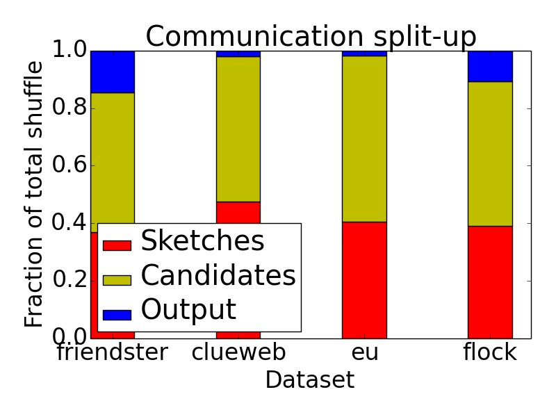
We split communication into three parts: the sketch shuffle, the candidate shuffle, and the final (deduped) output. The total of all these is presented in Tab. 2. (We stress that this is not shuffled together.) The split-up between the various parts is show in in Fig. 5. Observe that the sketch and candidate shuffle are roughly equal. For friendster and flock, the (deduped) output is itself more than 10% of the total shuffle. This (weakly) justifies the optimality Theorem 4.1 in these cases, since the total communication is at most an order of magnitude more than the desired output. For the other cases, the output is between 3-5% of the total shuffle.

Comparisons with existing art: No other algorithm works at this scale, and we were not able to deploy anything else for such large datasets. Nonetheless, given the parameters of the datasets, we can mathematically argue against other approaches.

• Wedge sampling of Cohen-Lewis [11], DISCO [43]: Distributed version of wedge sampling were given by Zadeh and Goel in their DISCO algorithm [43]. But it cannot scale to these sizes. DISCO is equivalent to using Round 2 of WHIMPto set up weights, and then running Round 3 without any filtering step (Step 1(b)v). Then, we would look for all pairs $(a,b)$ that have been emitted sufficiently many times, and make those the final output. In this case, CPU and shuffle costs are basically identical, since any candidate generated is emitted.

  Consider $(a,b)$ such that $A_{*,a}\cdot A_{*,b}=\tau$. By the wedge sampling calculations, $s\|A^{T}A\|_{1}$ wedge samples would generate $(a,b)$ an expected $s\tau$ times. We would need to ensure that this is concentrated well, since we finally output pairs generated often enough. In our experience, setting $s=50/\tau$ is the bare minimum to get precision/recall more than $0.8$. Note that WHIMP only needs to generate such a wedge sample once, since Step 1(b)v is then guaranteed to output it (assuming SimHash is accurate). But vanilla wedge sampling must generate $(a,b)$ with a frequency close to its expectation. Thus, WHIMP can set $s$ closer to (say) $10/\tau$, but this is not enough for the convergence of wedge sampling.

  But all the wedges have to be shuffled, and this leads to $10\|A^{T}A\|_{1}/\tau$ wedges being shuffled. Each wedge is two longs (using standard representations), and that gives a ballpark estimate of $160\|A^{T}A\|_{1}/\tau$. We definitely care about $\tau=0.2$, and WHIMP generates results for this setting (Fig. 3). We compute this value for the various datasets in Tab. 2, and present it as the estimated shuffle cost for DISCO.

  Observe that it is significantly large than the total shuffle cost of WHIMP, which is actually split roughly equally into two parts (Fig. 5). The wedge shuffles discussed above are most naturally done in a single round. To shuffle more than 200TB would require a more complex algorithm that splits the wedge samples into various rounds. For eu and flock, the numbers are more than 1000TB, and completely beyond the possibility of engineering. We note that friendster can probably be handled by the DISCO algorithm.

• Locality-Sensitive Hashing [24, 37]: LSH is an important method for nearest neighbor search. Unfortunately, it does not perform well when similarities are low but still significant (say $\tau=0.2$). Furthermore, it is well-known to require large memory overhead. The basic idea is to hash every vector into a “bucket” using, say, a small (like 8-bit) SimHash sketch. The similarity is explicitly computed on all pairs of vectors in a bucket, i.e. those with the same sketch value. This process is repeated with a large number of hash functions to ensure that most similar pairs are found.

  Using SimHash, the mathematics says roughly the following. (We refer the reader to important LSH papers for more details [24, 18, 3, 37].) Let the probability of two similar vectors (with cosine similarity above $0.2$) having the same SimHash value be denoted $P_{1}$. Let the corresponding probability for two vectors with similarity zero by $P_{2}$. By the SimHash calculations of §6, $P_{1}=1/2-\cos^{-1}(0.2)/\pi\approx 0.56$, while $P_{2}=0.5$. This difference measures the “gap" obtained by the SimHash function. The LSH formula basically tells us that the total storage of all the hashes is (at least) $n^{1+(\log P_{1})/(\log P_{2})}$ bytes. This comes out to be $n^{1.83}$. Assuming that $n$ is around 1 billion, the total storage is 26K TB. This is astronomically large, and even reducing this by a factor of hundred is insufficient for feasibility.

Table 3: Top similar results for a few Twitter accounts, generated from WHIMP on flock.

Users similar to @www2016ca
Rank	Twitter @handle	Score
1	@WSDMSocial	0.268
2	@WWWfirenze	0.213
3	@SIGIR2016	0.190
4	@ecir2016	0.175
5	@WSDM2015	0.155

Users similar to @duncanjwatts
Rank	Twitter @handle	Score
1	@ladamic	0.287
2	@davidlazer	0.286
3	@barabasi	0.284
4	@jure	0.218
5	@net_science	0.200

Users similar to @POTUS
Rank	Twitter @handle	Score
1	@FLOTUS	0.387
2	@HillaryClinton	0.368
3	@billclinton	0.308
4	@BernieSanders	0.280
5	@WhiteHouse	0.267

Case Study: In addition to the demonstration of the algorithm’s performance in terms of raw precision and recall, we also showcase some examples to illustrate the practical effectiveness of the approach. Some of these results are presented in Table 3. First, note that the cosine score values that generate the results are around 0.2, which provides justification for our focus on generating results with these values. Furthermore, note that even at these values, the results are quite interpretable and clearly find similar users: for the @www2016ca account, it finds accounts for other related social networks and data mining conferences. For @duncanjwatts, who is a network science researcher, the algorithm finds other network science researchers. And finally, an example of a very popular user is @POTUS, for whom the algorithm finds clearly very related accounts.

References

- [1] L. Adamic and E. Adar. Friends and neighbors on the web. Social Networks, 25(3):211–230, 2003.
- [2] R. R. Amossen and R. Pagh. Faster join-projects and sparse matrix multiplications. In ICDT ’09: Proc. 12th Intl. Conf. on Database Theory, pages 121–126, 2009.
- [3] A. Andoni and P. Indyk. Near-optimal hashing algorithms for approximate nearest neighbor in high dimensions. Comm. of the ACM, 1:117–122, 2008.
- [4] A. Andoni, P. Indyk, T. Laarhoven, I. P. Razenshteyn, and L. Schmidt. Practical and optimal LSH for angular distance. In Advances in Neural Information Processing Systems 28: Annual Conference on Neural Information Processing Systems 2015, December 7-12, 2015, Montreal, Quebec, Canada, pages 1225–1233, 2015.
- [5] F. Angiulli and C. Pizzuti. An approximate algorithm for top- closest pairs join query in large high dimensional data. Data & Knowledge Engineering, 53(3):263–281, June 2005.
- [6] G. Ballard, T. G. Kolda, A. Pinar, and C. Seshadhri. Diamond sampling for approximate maximum all-pairs dot-product (MAD) search. In International Conference on Data Mining, pages 11–20, 2015.
- [7] M.-A. Belabbas and P. Wolfe. On sparse representations of linear operators and the approximation of matrix products. In CISS 2008: 42nd Annual Conf. on Information Sciences and Systems, pages 258–263, Mar. 2008.
- [8] P. Boldi, M. Rosa, M. Santini, and S. Vigna. Layered label propagation: A multiresolution coordinate-free ordering for compressing social networks. In S. Srinivasan, K. Ramamritham, A. Kumar, M. P. Ravindra, E. Bertino, and R. Kumar, editors, Conference on World Wide Web (WWW), pages 587–596. ACM Press, 2011.
- [9] P. Boldi and S. Vigna. The WebGraph framework I: Compression techniques. In Conference on World Wide Web, pages 595–601, Manhattan, USA, 2004. ACM Press.
- [10] M. Charikar. Similarity estimation techniques from rounding algorithms. In Symposium on Theory of Computing, pages 380–388, 2002.
- [11] E. Cohen and D. D. Lewis. Approximating matrix multiplication for pattern recognition tasks. J. Algorithms, 30(2):211–252, 1999.
- [12] A. S. Das, M. Datar, A. Garg, and S. Rajaram. Google news personalization: scalable online collaborative filtering. In Proceedings of World Wide Web, pages 271–280, 2007.
- [13] T. Davis. Direct Methods for Sparse Linear Systems. SIAM, 2006.
- [14] J. Dean and S. Ghemawat. Mapreduce: simplified data processing on large clusters. Communications of the ACM, 51(1):107–113, 2008.
- [15] P. Drineas and R. Kannan. Fast monte-carlo algorithms for approximate matrix multiplication. In FoCS’01: Proc. 42nd IEEE Symposium on Foundations of Computer Science, pages 452–459, Oct. 2001.
- [16] P. Drineas, R. Kannan, and M. W. Mahoney. Fast Monte Carlo algorithms for matrices I: Approximating matrix multiplication. SIAM Journal on Computing, 36(1):132–157, Jan. 2006.
- [17] P. Drineas and M. W. Mahoney. On the Nyström method for approximating a gram matrix for improved kernel-based learning. J. Mach. Learn. Res., 6:2153–2175, Dec. 2005.
- [18] A. Gionis, P. Indyk, and R. Motwani. Similarity search in high dimensions via hashing. In Proceedings of VLDB, pages 518–529, 1999.
- [19] A. Goel and K. Munagala. Complexity measures for map-reduce, and comparison to parallel computing. arXiv preprint arXiv:1211.6526, 2012.
- [20] A. Goel, A. Sharma, D. Wang, and Z. Yin. Discovering similar users on twitter. In 11th Workshop on Mining and Learning with Graphs, 2013.
- [21] P. Gupta, A. Goel, J. J. Lin, A. Sharma, D. Wang, and R. Zadeh. WTF: the who to follow service at twitter. In Conference on World Wide Web, pages 505–514, 2013.
- [22] F. G. Gustavson. Two fast algorithms for sparse matrices: Multiplication and permuted transposition. ACM Transactions on Mathematical Software, 4(3):250–269, Sept. 1978.
- [23] J. T. Holodnak and I. C. F. Ipsen. Randomized approximation of the gram matrix: Exact computation and probabilistic bounds. SIAM Journal on Matrix Analysis and Applications, 36(1):110–137, 2015.
- [24] P. Indyk and R. Motwani. Approximate nearest neighbors: Towards removing the curse of dimensionality. In Proceedings of STOC, pages 604–613, 1998.
- [25] Intel. Math kernel library reference manual, 2014. Version 11.2.
- [26] D. V. Kalashnikov, S. Mehrotra, and Z. Chen. Exploiting relationships for domain-independent data cleaning. In SDM’05: Proc. 2005 SIAM Intl. Conf. on Data Mining, pages 262–273, Apr. 2005.
- [27] G. Lee, J. Lin, C. Liu, A. Lorek, and D. Ryaboy. The unified logging infrastructure for data analytics at twitter. Proceedings of the VLDB Endowment, 5(12):1771–1780, 2012.
- [28] J. Leskovec and A. Krevl. SNAP Datasets: Stanford large network dataset collection. http://snap.stanford.edu/data, June 2014.
- [29] J. Leskovec, A. Rajaraman, and J. D. Ullman. Mining of massive datasets. Cambridge University Press, 2014.
- [30] D. Liben-Nowell and J. Kleinberg. The link prediction problem for social networks. Journal of the American Society for Information Science and Technology, 58(7):1019–1031, 2007.
- [31] J. Lin and D. Ryaboy. Scaling big data mining infrastructure: the twitter experience. ACM SIGKDD Explorations Newsletter, 14(2):6–19, 2013.
- [32] A. Magen and A. Zouzias. Low rank matrix-valued Chernoff bounds and approximate matrix multiplication. In Proc. Symposium on Discrete Algorithms (SODA), pages 1422–1436, 2011.
- [33] M. McPherson, L. Smith-Lovin, and J. M. Cook. Birds of a feather: Homophily in social networks. Annual review of sociology, pages 415–444, 2001.
- [34] R. Pagh. Compressed matrix multiplication. ACM Transactions on Computation Theory (TOCT), 5(3):1–17, Aug. 2013.
- [35] F. Ricci, L. Rokach, and B. Shapira. Introduction to recommender systems handbook. Springer, 2011.
- [36] T. Sarlós. Improved approximation algorithms for large matrices via random projections. In Proceedings of Foundations of Computer Science, pages 143–152, Oct. 2006.
- [37] A. Shrivastava and P. Li. Asymmetric LSH (ALSH) for sublinear time maximum inner product search (MIPS). In NIPS 2014: Advances in Neural Information Processing Systems 27, pages 2321–2329, 2014.
- [38] A. Shrivastava and P. Li. Asymmetric minwise hashing for indexing binary inner products and set containment. In Conference on World Wide Web (WWW), pages 981–991, 2015.
- [39] A. Shrivastava and P. Li. Improved asymmetric locality sensitive hashing (ALSH) for maximum inner product search (MIPS). In Conference on Uncertainty in Artificial Intelligence (UAI), pages 812–821, 2015.
- [40] K. Shvachko, H. Kuang, S. Radia, and R. Chansler. The hadoop distributed file system. In 2010 IEEE 26th symposium on mass storage systems and technologies (MSST), pages 1–10. IEEE, 2010.
- [41] R. Xiang, J. Neville, and M. Rogati. Modeling relationship strength in online social networks. In Proceedings of the 19th international conference on World wide web, pages 981–990. ACM, 2010.
- [42] X. Yan, P. S. Yu, and J. Han. Substructure similarity search in graph databases. In Proceedings of the 2005 ACM SIGMOD international conference on Management of data, pages 766–777. ACM, 2005.
- [43] R. B. Zadeh and A. Goel. Dimension independent similarity computation. Journal of Machine Learning Research, 14(1):1605–1626, 2013.