Active Learning for Cost-Sensitive Classification

Abstract

We design an active learning algorithm for cost-sensitive multiclass classification: problems where different errors have different costs. Our algorithm, COAL, makes predictions by regressing to each label’s cost and predicting the smallest. On a new example, it uses a set of regressors that perform well on past data to estimate possible costs for each label. It queries only the labels that could be the best, ignoring the sure losers. We prove COAL can be efficiently implemented for any regression family that admits squared loss optimization; it also enjoys strong guarantees with respect to predictive performance and labeling effort. We empirically compare COAL to passive learning and several active learning baselines, showing significant improvements in labeling effort and test cost on real-world datasets.

1 Introduction

The field of active learning studies how to efficiently elicit relevant information so learning algorithms can make good decisions. Almost all active learning algorithms are designed for binary classification problems, leading to the natural question: How can active learning address more complex prediction problems? Multiclass and importance-weighted classification require only minor modifications but we know of no active learning algorithms that enjoy theoretical guarantees for more complex problems.

One such problem is cost-sensitive multiclass classification (CSMC). In CSMC with $K$ classes, passive learners receive input examples $x$ and cost vectors $c\in\mathbb{R}^{K}$, where $c(y)$ is the cost of predicting label $y$ on $x$. A natural design for an active CSMC learner then is to adaptively query the costs of only a (possibly empty) subset of labels on each $x$. Since measuring label complexity is more nuanced in CSMC (e.g., is it more expensive to query three costs on a single example or one cost on three examples?), we track both the number of examples for which at least one cost is queried, along with the total number of cost queries issued. The first corresponds to a fixed human effort for inspecting the example. The second captures the additional effort for judging the cost of each prediction, which depends on the number of labels queried. (By querying a label, we mean querying the cost of predicting that label given an example.)

In this setup, we develop a new active learning algorithm for CSMC called Cost Overlapped Active Learning (COAL). COAL assumes access to a set of regression functions, and, when processing an example $x$, it uses the functions with good past performance to compute the range of possible costs that each label might take. Naturally, COAL only queries labels with large cost range, akin to uncertainty-based approaches in active regression [11], but furthermore, it only queries labels that could possibly have the smallest cost, avoiding the uncertain, but surely suboptimal labels. The key algorithmic innovation is an efficient way to compute the cost range realized by good regressors. This computation, and COAL as a whole, only requires that the regression functions admit efficient squared loss optimization, in contrast with prior algorithms that require 0/1 loss optimization [7, 19].

Among our results, we prove that when processing $n$ (unlabeled) examples with $K$ classes and a regression class with pseudo-dimension $d$ (See Definition 1),

1. The algorithm needs to solve $\mathcal{O}(Kn^{5})$ regression problems over the function class (Corollary 2). Thus COAL runs in polynomial time for convex regression sets.

2. With no assumptions on the noise in the problem, the algorithm achieves generalization error $\tilde{\mathcal{O}}(\sqrt{Kd/n})$ and requests $\tilde{\mathcal{O}}(n\theta_{2}\sqrt{Kd})$ costs from $\tilde{\mathcal{O}}(n\theta_{1}\sqrt{Kd})$ examples (Theorems 3 and 6) where $\theta_{1},\theta_{2}$ are the disagreement coefficients (Definition 2). The worst case offers minimal improvement over passive learning, akin to active learning for binary classification.

3. With a Massart-type noise assumption (Assumption 3), the algorithm has generalization error $\tilde{\mathcal{O}}(Kd/n)$ while requesting $\tilde{\mathcal{O}}(Kd(\theta_{2}+K\theta_{1})\log n)$ labels from $\tilde{\mathcal{O}}(Kd\theta_{1}\log n)$ examples (Corollary 4, Theorem 7). Thus under favorable conditions, COAL requests exponentially fewer labels than passive learning.

We also derive generalization and label complexity bounds under a milder Tsybakov-type noise condition (Assumption 4). Existing lower bounds from binary classification [19] suggest that our results are optimal in their dependence on $n$, although these lower bounds do not directly apply to our setting. We also discuss some intuitive examples highlighting the benefits of using COAL.

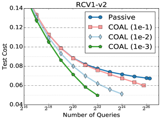
Figure 1: Empirical evaluation of COAL on Reuters text categorization dataset. Active learning achieves better test cost than passive, with a factor of $16$ fewer queries. See Section 7 for details.

CSMC provides a more expressive language for success and failure than multiclass classification, which allows learning algorithms to make the trade-offs necessary for good performance and broadens potential applications. For example, CSMC can naturally express partial failure in hierarchical classification [41]. Experimentally, we show that COAL substantially outperforms the passive learning baseline with orders of magnitude savings in the labeling effort on a number of hierarchical classification datasets (see Figure 1 for comparison between passive learning and COAL on Reuters text categorization).

CSMC also forms the basis of learning to avoid cascading failures in joint prediction tasks like structured prediction and reinforcement learning [15, 37, 13]. As our second application, we consider learning to search algorithms for joint or structured prediction, which operate by a reduction to CSMC. In this reduction, evaluating the cost of a class often involves a computationally expensive “roll-out,” so using an active learning algorithm inside such a passive joint prediction method can lead to significant computational savings. We show that using COAL within the Aggravate algorithm [37, 13] reduces the number of roll-outs by a factor of $\frac{1}{4}$ to $\frac{3}{4}$ on several joint prediction tasks.

Our code is publicly available as part of the Vowpal Wabbit machine learning library.

2 Related Work

Active learning is a thriving research area with many theoretical and empirical studies. We recommend the survey of Settles [39] for an overview of more empirical research. We focus here on theoretical results.

Our work falls into the framework of disagreement-based active learning, which studies general hypothesis spaces typically in an agnostic setup (see Hanneke [19] for an excellent survey). Existing results study binary classification, while our work generalizes to CSMC, assuming that we can accurately predict costs using regression functions from our class. One difference that is natural for CSMC is that our query rule checks the range of predicted costs for a label.

The other main difference is that we use a square loss oracle to search the version space. In contrast, prior work either explicitly enumerates the version space [5, 46] or uses a 0/1 loss classification oracle for the search [14, 7, 8, 24]. In most instantiations, the oracle solves an NP-hard problem and so does not directly lead to an efficient algorithm, although practical implementations using heuristics are still quite effective. Our approach instead uses a squared-loss regression oracle, which can be implemented efficiently via convex optimization and leads to a polynomial time algorithm.

In addition to disagreement-based approaches, much research has focused on plug-in rules for active learning in binary classification, where one estimates the class-conditional regression function [10, 32, 20, 9]. Apart from Hanneke and Yang [20], these works make smoothness assumptions and have a nonparametric flavor. Instead, Hanneke and Yang [20] assume a calibrated surrogate loss and abstract realizable function class, which is more similar to our setting. While the details vary, our work and these prior results employ the same algorithmic recipe of maintaining an implicit version space and querying in a suitably-defined disagreement region. Our work has two notable differences: (1) our algorithm operates in an oracle computational model, only accessing the function class through square loss minimization problems, (2) our results apply to general CSMC, which exhibit significant differences from binary classification. See Subsection 6.1 for further discussion.

Focusing on linear representations, Balcan et al. [6], Balcan and Long [4] study active learning with distributional assumptions, while the selective sampling framework from the online learning community considers adversarial assumptions [12, 16, 33, 1]. These methods use query strategies that are specialized to linear representations and do not naturally generalize to other hypothesis classes.

Supervised learning oracles that solve NP-hard optimization problems in the worst case have been used in other problems including contextual bandits [2, 43] and structured prediction [15]. Thus we hope that our work can inspire new algorithms for these settings as well.

Lastly, we mention that square loss regression has been used to estimate costs for passive CSMC [27], but, to our knowledge, using a square loss oracle for active CSMC is new.

Advances over Krishnamurthy et al. [26].

Active learning for CSMC was introduced recently in Krishnamurthy et al. [26] with an algorithm that also uses cost ranges to decide where to query. They compute cost ranges by using the regression oracle to perform a binary search for the maximum and minimum costs, but this computation results in a sub-optimal label complexity bound. We resolve this sub-optimality with a novel cost range computation that is inspired by the multiplicative weights technique for solving linear programs. This algorithmic improvement also requires a significantly more sophisticated statistical analysis for which we derive a novel uniform Freedman-type inequality for classes with bounded pseudo-dimension. This result may be of independent interest.

Krishnamurthy et al. [26] also introduce an online approximation for additional scalability and use this algorithm for their experiments. Our empirical results use this same online approximation and are slightly more comprehensive. Finally, we also derive generalization and label complexity bounds for our algorithm in a setting inspired by Tsybakov’s low noise condition [30, 45].

Comparison with Foster et al. [18].

In a follow-up to the present paper, Foster et al. [18] build on our work with a regression-based approach for contextual bandit learning, a problem that bears some similarities to active learning for CSMC. The results are incomparable due to the differences in setting, but it is worth discussing their techniques. As in our paper, Foster et al. [18] maintain an implicit version space and compute maximum and minimum costs for each label, which they use to make predictions. They resolve the sub-optimality in Krishnamurthy et al. [26] with epoching, which enables a simpler cost range computation than our multiplicative weights approach. However, epoching incurs an additional $\log(n)$ factor in the label complexity, and under low-noise conditions where the overall bound is $\mathcal{O}(\textrm{polylog}(n))$, this yields a polynomially worse guarantee than ours.

3 Problem Setting and Notation

We study cost-sensitive multiclass classification (CSMC) problems with $K$ classes, where there is an instance space $\mathcal{X}$, a label space $\mathcal{Y}=\{1,\ldots,K\}$, and a distribution $\mathcal{D}$ supported on $\mathcal{X}\times[0,1]^{K}$. If $(x,c)\sim\mathcal{D}$, we refer to $c$ as the cost-vector, where $c(y)$ is the cost of predicting $y\in\mathcal{Y}$. A classifier $h:\mathcal{X}\rightarrow\mathcal{Y}$ has expected cost $\mathbb{E}_{(x,c)\sim\mathcal{D}}[c(h(x))]$ and we aim to find a classifier with minimal expected cost.

Let $\mathcal{G}\triangleq\{g:\mathcal{X}\mapsto[0,1]\}$ denote a set of base regressors and let $\mathcal{F}\triangleq\mathcal{G}^{K}$ denote a set of vector regressors where the $y^{\textrm{th}}$ coordinate of $f\in\mathcal{F}$ is written as $f(\cdot;y)$. The set of classifiers under consideration is $\mathcal{H}\triangleq\{h_{f}\mid f\in\mathcal{F}\}$ where each $f$ defines a classifier $h_{f}:\mathcal{X}\mapsto\mathcal{Y}$ by

$$h_{f}(x)\triangleq\mathop{\mathrm{argmin}}_{y}f(x;y).$$ (1)

When using a set of regression functions for a classification task, it is natural to assume that the expected costs under $\mathcal{D}$ can be predicted by some function in the set. This motivates the following realizability assumption.

Assumption 1 (Realizability).

Define the Bayes-optimal regressor $f^{\star}$, which has $f^{\star}(x;y)\triangleq\mathbb{E}_{c}[c(y)|x],\forall x\in\mathcal{X}$ (with $\mathcal{D}(x)>0$), $y\in\mathcal{Y}$. We assume that $f^{\star}\in\mathcal{F}$.

While $f^{\star}$ is always well defined, note that the cost itself may be noisy. In comparison with our assumption, the existence of a zero-cost classifier in $\mathcal{H}$ (which is often assumed in active learning) is stronger, while the existence of $h_{f^{\star}}$ in $\mathcal{H}$ is weaker but has not been leveraged in active learning.

We also require assumptions on the complexity of the class $\mathcal{G}$ for our statistical analysis. To this end, we assume that $\mathcal{G}$ is a compact convex subset of $L_{\infty}(\mathcal{X})$ with finite pseudo-dimension, which is a natural extension of VC-dimension for real-valued predictors.

Definition 1 (Pseudo-dimension).

The pseudo-dimension $\mathrm{Pdim}(\mathcal{F})$ of a function class $\mathcal{F}:\mathcal{X}\rightarrow\mathbb{R}$ is defined as the VC-dimension of the set of threshold functions $\mathcal{H}^{+}\triangleq\{(x,\xi)\mapsto{\bf 1}\{f(x)>\xi\}:f\in\mathcal{F}\}\subset\mathcal{X}\times\mathbb{R}\rightarrow\{0,1\}$.

Assumption 2.

We assume that $\mathcal{G}$ is a compact convex set with $\mathrm{Pdim}(\mathcal{G})=d<\infty$.

As an example, linear functions in some basis representation, e.g., $g(x)=\sum_{i=1}^{d}w_{i}\phi_{i}(x)$, where weights $w_{i}$ are bounded in some norm, have pseudodimension $d$. In fact, our result can be stated entirely in terms of covering numbers, and we translate to pseudo-dimension using the fact that such classes have “parametric" covering numbers of the form $(1/\varepsilon)^{d}$. Thus, our results extend to classes with “nonparametric" growth rates as well (e.g., Holder-smooth functions), although we focus on the parametric case for simplicity. Note that this is a significant departure from Krishnamurthy et al. [26], which assumed that $\mathcal{G}$ was finite.

Our assumption that $\mathcal{G}$ is a compact convex set introduces a computational challenging of managing this infinitely large set. To address this challenge, we follow the trend in active learning of leveraging existing algorithmic research on supervised learning [14, 8, 7] and access $\mathcal{G}$ exclusively through a regression oracle. Given an importance-weighted dataset $D=\{x_{i},c_{i},w_{i}\}_{i=1}^{n}$ where $x_{i}\in\mathcal{X},c_{i}\in\mathbb{R},w_{i}\in\mathbb{R}_{+}$, the regression oracle computes

$$\textsc{Oracle}(D)\in\mathop{\mathrm{argmin}}_{g\in\mathcal{G}}\sum_{i=1}^{n}w_{i}(g(x_{i})-c_{i})^{2}.$$ (2)

Since we assume that $\mathcal{G}$ is a compact convex set it is amenable to standard convex optimization techniques, so this imposes no additional restriction. However, in the special case of linear functions, this optimization is just least squares and can be computed in closed form. Note that this is fundamentally different from prior works that use a 0/1-loss minimization oracle [14, 8, 7], which involves an NP-hard optimization in most cases of interest.

Remark 1.

Our assumption that $\mathcal{G}$ is convex is only for computational tractability, as it is crucial in the efficient implementation of our query strategy, but is not required for our generalization and label complexity bounds. Unfortunately recent guarantees for learning with non-convex classes [29, 36] do not immediately yield efficient active learning strategies. Note also that Krishnamurthy et al. [26] obtain an efficient algorithm without convexity, but this yields a suboptimal label complexity guarantee.

Given a set of examples and queried costs, we often restrict attention to regression functions that predict these costs well and assess the uncertainty in their predictions given a new example $x$. For a subset of regressors $G\subset\mathcal{G}$, we measure uncertainty over possible cost values for $x$ with

$$\gamma(x,G) \triangleq c_{+}(x,G)-c_{-}(x,G),\qquad c_{+}(x,G)\triangleq\max_{g\in G}g(x),\qquad c_{-}(x,G)\triangleq\min_{g\in G}g(x).$$ (3)

For vector regressors $F\subset\mathcal{F}$, we define the cost range for a label $y$ given $x$ as $\gamma(x,y,F)\triangleq\gamma(x,G_{F}(y))$ where $G_{F}(y)\triangleq\{f(\cdot;y)~{}|~{}f\in F\}$ are the base regressors induced by $F$ for $y$. Note that since we are assuming realizability, whenever $f^{\star}\in F$, the quantities $c_{+}(x,G_{F}(y))$ and $c_{-}(x,G_{F}(y))$ provide valid upper and lower bounds on $\mathbb{E}[c(y)|x]$.

To measure the labeling effort, we track the number of examples for which even a single cost is queried as well as the total number of queries. This bookkeeping captures settings where the editorial effort for inspecting an example is high but each cost requires minimal further effort, as well as those where each cost requires substantial effort. Formally, we define $Q_{i}(y)\in\{0,1\}$ to be the indicator that the algorithm queries label $y$ on the $i^{\textrm{th}}$ example and measure

$$L_{1}\triangleq\sum_{i=1}^{n}\bigvee_{y}Q_{i}(y),\textrm{ and }L_{2}\triangleq\sum_{i=1}^{n}\sum_{y}Q_{i}(y).$$ (4)

4 Cost Overlapped Active Learning

Algorithm 1 Cost Overlapped Active Learning (COAL)

1:Input: Regressors $\mathcal{G}$, failure probability $\delta\leq 1/e$.

2:Set $\psi_{i}=1/\sqrt{i}$, $\kappa=3$, $\nu_{n}=324(d\log(n)+\log(8Ke(d+1)n^{2}/\delta))$.

3:Set $\Delta_{i}=\kappa\min\{\frac{\nu_{n}}{i-1},1\}$.

4:for $i=1,2,\ldots,n$ do

5:     $g_{i,y}\leftarrow\arg\min_{g\in\mathcal{G}}\widehat{R}_{i}(g;y)$. (See (5)).

6:     Define $f_{i}\leftarrow\{g_{i,y}\}_{y=1}^{K}$.

7:     (Implicitly define) $\mathcal{G}_{i}(y)\leftarrow\{g\in\mathcal{G}_{i-1}(y)\mid\widehat{R}_{i}(g;y)\leq\widehat{R}_{i}(g_{i,y};y)+\Delta_{i}\}$.

8:     Receive new example $x$. $Q_{i}(y)\leftarrow 0,\forall y\in\mathcal{Y}$.

9:     for every $y\in\mathcal{Y}$ do

10:         $\widehat{c_{+}}(y)\leftarrow\textsc{MaxCost}((x,y),\psi_{i}/4)$ and $\widehat{c_{-}}(y)\leftarrow\textsc{MinCost}((x,y),\psi_{i}/4)$.

11:     end for

12:     $Y^{\prime}\leftarrow\{y\in\mathcal{Y}\mid\widehat{c_{-}}(y)\leq\min_{y^{\prime}}\widehat{c_{+}}(y^{\prime})\}.$

13:     if $|Y^{\prime}|>1$ then

14:         $Q_{i}(y)\leftarrow 1$ if $y\in Y^{\prime}$ and $\widehat{c_{+}}(y)-\widehat{c_{-}}(y)>\psi_{i}$.

15:     end if

16:     Query costs of each $y$ with $Q_{i}(y)=1$.

17:end for

The pseudocode for our algorithm, Cost Overlapped Active Learning (COAL), is given in Algorithm 1. Given an example $x$, COAL queries the costs of some of the labels $y$ for $x$. These costs are chosen by (1) computing a set of good regression functions based on the past data (i.e., the version space), (2) computing the range of predictions achievable by these functions for each $y$, and (3) querying each $y$ that could be the best label and has substantial uncertainty. We now detail each step.

To compute an approximate version space we first find the regression function that minimizes the empirical risk for each label $y$, which at round $i$ is:

$$\widehat{R}_{i}(g;y)\triangleq\frac{1}{i-1}\sum_{j=1}^{i-1}(g(x_{j})-c_{j}(y))^{2}Q_{j}(y).$$ (5)

Recall that $Q_{j}(y)$ is the indicator that we query label $y$ on the $j^{\textrm{th}}$ example. Computing the minimizer requires one oracle call. We implicitly construct the version space $\mathcal{G}_{i}(y)$ in Line 7 as the surviving regressors with low square loss regret to the empirical risk minimizer. The tolerance on this regret is $\Delta_{i}$ at round $i$, which scales like $\tilde{\mathcal{O}}(d/i)$, where recall that $d$ is the pseudo-dimension of the class $\mathcal{G}$.

COAL then computes the maximum and minimum costs predicted by the version space $\mathcal{G}_{i}(y)$ on the new example $x$. Since the true expected cost is $f^{\star}(x;y)$ and, as we will see, $f^{\star}(\cdot;y)\in\mathcal{G}_{i}(y)$, these quantities serve as a confidence bound for this value. The computation is done by the MaxCost and MinCost subroutines which produce approximations to $c_{+}(x,\mathcal{G}_{i}(y))$ and $c_{-}(x,\mathcal{G}_{i}(y))$ respectively (See (3)).

Finally, using the predicted costs, COAL issues (possibly zero) queries. The algorithm queries any non-dominated label that has a large cost range, where a label is non-dominated if its estimated minimum cost is smaller than the smallest maximum cost (among all other labels) and the cost range is the difference between the label’s estimated maximum and minimum costs.

Intuitively, COAL queries the cost of every label which cannot be ruled out as having the smallest cost on $x$, but only if there is sufficient ambiguity about the actual value of the cost. The idea is that labels with little disagreement do not provide much information for further reducing the version space, since by construction all regressors would suffer similar square loss. Moreover, only the labels that could be the best need to be queried at all, since the cost-sensitive performance of a hypothesis $h_{f}$ depends only on the label that it predicts. Hence, labels that are dominated or have small cost range need not be queried.

Similar query strategies have been used in prior works on binary and multiclass classification [33, 16, 1], but specialized to linear representations. The key advantage of the linear case is that the set $\mathcal{G}_{i}(y)$ (formally, a different set with similar properties) along with the maximum and minimum costs have closed form expressions, so that the algorithms are easily implemented. However, with a general set $\mathcal{G}$ and a regression oracle, computing these confidence intervals is less straightforward. We use the MaxCost and MinCost subroutines, and discuss this aspect of our algorithm next.

4.1 Efficient Computation of Cost Range

Algorithm 2 MaxCost

1:Input: $(x,y)$, tolerance tol, (implicitly) risk functionals $\{\widehat{R}_{j}(\cdot;y)\}_{j=1}^{i}$.

2:Compute $g_{j,y}=\mathop{\mathrm{argmin}}_{g\in\mathcal{G}}\widehat{R}_{j}(g;y)$ for each $j$.

3:Let $\Delta_{j}=\kappa\min\{\frac{\nu_{n}}{j-1},1\}$, $\tilde{\Delta}_{j}=\widehat{R}_{j}(g_{j,y};y)+\Delta_{j}$ for each $j$.

4:Initialize parameters: $c_{\ell}\leftarrow 0,c_{h}\leftarrow 1,T\leftarrow\frac{\log(i+1)(12/\Delta_{i})^{2}}{\textsc{tol}^{4}},\eta\leftarrow\sqrt{\log(i+1)/T}$.

5:while $|c_{\ell}-c_{h}|>\textsc{tol}^{2}/2$ do

6:     $c\leftarrow\frac{c_{h}-c_{\ell}}{2}$

7:     $\mu^{(1)}\leftarrow{\bf 1}\in\mathbb{R}^{i+1}$. $\triangleright$ Use MW to check feasibility of Program (9).

8:     for $t=1,\ldots,T$ do

9:         Use the regression oracle to find

$$g_{t}\leftarrow\mathop{\mathrm{argmin}}_{g\in\mathcal{G}}\mu^{(t)}_{0}(g(x)-1)^{2}+\sum_{j=1}^{i}\mu^{(t)}_{j}\widehat{R}_{j}(g;y)$$ (6)

10:         If the objective in (6) for $g_{t}$ is at least $\mu^{(t)}_{0}c+\sum_{j=1}^{i}\mu^{(t)}_{j}\tilde{\Delta}_{j}$, $c_{\ell}\leftarrow c$, go to 5.

11:         Update

$$\mu^{(t+1)}_{j}\leftarrow\mu^{(t)}_{j}\left(1-\eta\frac{\tilde{\Delta}_{j}-\widehat{R}_{j}(g_{t};y)}{\Delta_{j}+1}\right),\quad\mu_{0}^{(t+1)}\leftarrow\mu_{0}^{(t)}\left(1-\eta\frac{c-(g_{t}(x)-1)^{2}}{2}\right).$$

12:     end for

13:     $c_{h}\leftarrow c$.

14:end while

15:Return $\widehat{c_{+}}(y)=1-\sqrt{c_{\ell}}$.

In this section, we describe the MaxCost subroutine which uses the regression oracle to approximate the maximum cost on label $y$ realized by $\mathcal{G}_{i}(y)$, as defined in (3). The minimum cost computation requires only minor modifications that we discuss at the end of the section.

Describing the algorithm requires some additional notation. Let $\tilde{\Delta}_{j}\triangleq\Delta_{j}+\widehat{R}_{j}(g_{j,y};y)$ be the right hand side of the constraint defining the version space at round $j$, where $g_{j,y}$ is the ERM at round $j$ for label $y$, $\widehat{R}_{j}(\cdot;y)$ is the risk functional, and $\Delta_{j}$ is the radius used in COAL. Note that this quantity can be efficiently computed since $g_{j,y}$ can be found with a single oracle call. Due to the requirement that $g\in\mathcal{G}_{i-1}(y)$ in the definition of $\mathcal{G}_{i}(y)$, an equivalent representation is $\mathcal{G}_{i}(y)=\bigcap_{j=1}^{i}\{g:\widehat{R}_{j}(g;y)\leq\tilde{\Delta}_{j}\}$. Our approach is based on the observation that given an example $x$ and a label $y$ at round $i$, finding a function $g\in\mathcal{G}_{i}(y)$ which predicts the maximum cost for the label $y$ on $x$ is equivalent to solving the minimization problem:

$$\textrm{minimize}_{g\in\mathcal{G}}(g(x)-1)^{2}\quad\textrm{ such that }\quad\forall 1\leq j\leq i,\widehat{R}_{j}(g;y)\leq\tilde{\Delta}_{j}.$$ (7)

Given this observation, our strategy will be to find an approximate solution to the problem (7) and it is not difficult to see that this also yields an approximate value for the maximum predicted cost on $x$ for the label $y$.

In Algorithm 2, we show how to efficiently solve this program using the regression oracle. We begin by exploiting the convexity of the set $\mathcal{G}$, meaning that we can further rewrite the optimization problem (7) as

$$\textrm{minimize}_{P\in\Delta(\mathcal{G})}\mathbb{E}_{g\sim P}\left[(g(x)-1)^{2}\right]\quad\textrm{ such that }\quad\forall 1\leq j\leq i,\mathbb{E}_{g\sim P}\left[\widehat{R}_{j}(g;y)\right]\leq\tilde{\Delta}_{j}.$$ (8)

The above rewriting is effectively cosmetic as $\mathcal{G}=\Delta(\mathcal{G})$ by the definition of convexity, but the upshot is that our rewriting results in both the objective and constraints being linear in the optimization variable $P$. Thus, we effectively wish to solve a linear program in $P$, with our computational tool being a regression oracle over the set $\mathcal{G}$. To do this, we create a series of feasibility problems, where we repeatedly guess the optimal objective value for the problem (8) and then check whether there is indeed a distribution $P$ which satisfies all the constraints and gives the posited objective value. That is, we check

$$?\exists P\in\Delta(\mathcal{G})\textrm{ such that }\mathbb{E}_{g\sim P}(g(x)-1)^{2}\leq c\textrm{ and }\forall 1\leq j\leq i,\mathbb{E}_{g\sim P}\widehat{R}_{j}(g;y)\leq\tilde{\Delta}_{j}.$$ (9)

If we find such a solution, we increase our guess, and otherwise we reduce the guess and proceed until we localize the optimal value to a small enough interval.

It remains to specify how to solve the feasibility problem (9). Noting that this is a linear feasibility problem, we jointly invoke the Multiplicative Weights (MW) algorithm and the regression oracle in order to either find an approximately feasible solution or certify the problem as infeasible. MW is an iterative algorithm that maintains weights $\mu$ over the constraints. At each iteration it (1) collapses the constraints into one, by taking a linear combination weighted by $\mu$, (2) checks feasibility of the simpler problem with a single constraint, and (3) if the simpler problem is feasible, it updates the weights using the slack of the proposed solution. Details of steps (1) and (3) are described in Algorithm 2.

For step (2), the simpler problem that we must solve takes the form

$$?\exists P\in\Delta(\mathcal{G})\textrm{ such that }\mu_{0}\mathbb{E}_{g\sim P}(g(x)-1)^{2}+\sum_{j=1}^{i}\mu_{j}\mathbb{E}_{g\sim P}\widehat{R}_{j}(g;y)\leq\mu_{0}c+\sum_{j=1}^{i}\mu_{j}\tilde{\Delta}_{j}.$$

This program can be solved by a single call to the regression oracle, since all terms on the left-hand-side involve square losses while the right hand side is a constant. Thus we can efficiently implement the MW algorithm using the regression oracle. Finally, recalling that the above description is for a fixed value of objective $c$, and recalling that the maximum can be approximated by a binary search over $c$ leads to an oracle-based algorithm for computing the maximum cost. For this procedure, we have the following computational guarantee.

Theorem 1.

Algorithm 2 returns an estimate $\widehat{c_{+}}(x;y)$ such that $c_{+}(x;y)\leq\widehat{c_{+}}(x;y)\leq c_{+}(x;y)+\textsc{tol}$ and runs in polynomial time with $\mathcal{O}(\max\{1,i^{2}/\nu_{n}^{2}\}\log(i)\log(1/\textsc{tol})/\textsc{tol}^{4})$ calls to the regression oracle.

The minimum cost can be estimated in exactly the same way, replacing the objective $(g(x)-1)^{2}$ with $(g(x)-0)^{2}$ in Program (7). In COAL, we set $\textsc{tol}=1/\sqrt{i}$ at iteration $i$ and have $\nu_{n}=\tilde{\mathcal{O}}(d)$. As a consequence, we can bound the total oracle complexity after processing $n$ examples.

Corollary 2.

After processing $n$ examples, COAL makes $\tilde{\mathcal{O}}(K(d^{3}+n^{5}/d^{2}))$ calls to the square loss oracle.

Thus COAL can be implemented in polynomial time for any set $\mathcal{G}$ that admits efficient square loss optimization. Compared to Krishnamurthy et al. [26] which required $\mathcal{O}(n^{2})$ oracle calls, the guarantee here is, at face value, worse, since the algorithm is slower. However, the algorithm enforces a much stronger constraint on the version space which leads to a much better statistical analysis, as we will discuss next. Nevertheless, these algorithms that use batch square loss optimization in an iterative or sequential fashion are too computational demanding to scale to larger problems. Our implementation alleviates this with an alternative heuristic approximation based on a sensitivity analysis of the oracle, which we detail in Section 7.

5 Generalization Analysis

In this section, we derive generalization guarantees for COAL. We study three settings: one with minimal assumptions and two low-noise settings.

Our first low-noise assumption is related to the Massart noise condition [31], which in binary classification posits that the Bayes optimal predictor is bounded away from $1/2$ for all $x$. Our condition generalizes this to CSMC and posits that the expected cost of the best label is separated from the expected cost of all other labels.

Assumption 3.

A distribution $\mathcal{D}$ supported over $(x,c)$ pairs satisfies the Massart noise condition with parameter $\tau>0$, if for all $x$ (with $\mathcal{D}(x)>0$),

$$f^{\star}(x;y^{\star}(x))\leq\min_{y\neq y^{\star}(x)}f^{\star}(x;y)-\tau,$$

where $y^{\star}(x)\triangleq\mathop{\textrm{argmin}}_{y}f^{\star}(x;y)$ is the true best label for $x$.

The Massart noise condition describes favorable prediction problems that lead to sharper generalization and label complexity bounds for COAL. We also study a milder noise assumption, inspired by the Tsybakov condition [30, 45], again generalized to CSMC. See also Agarwal [1].

Assumption 4.

A distribution $\mathcal{D}$ supported over $(x,c)$ pairs satisfies the Tsbyakov noise condition with parameters $(\tau_{0},\alpha,\beta)$ if for all $0\leq\tau\leq\tau_{0}$,

$$\mathbb{P}_{x\sim\mathcal{D}}\left[\min_{y\neq y^{\star}(x)}f^{\star}(x;y)-f^{\star}(x;y^{\star}(x))\leq\tau\right]\leq\beta\tau^{\alpha},$$

where $y^{\star}(x)\triangleq\mathop{\textrm{argmin}}_{y}f^{\star}(x;y)$.

Observe that the Massart noise condition in Assumption 3 is a limiting case of the Tsybakov condition, with $\tau=\tau_{0}$ and $\alpha\rightarrow\infty$. The Tsybakov condition states that it is polynomially unlikely for the cost of the best label to be close to the cost of the other labels. This condition has been used in previous work on cost-sensitive active learning [1] and is also related to the condition studied by Castro and Nowak [10] with the translation that $\alpha=\frac{1}{\kappa-1}$, where $\kappa\in[0,1]$ is their noise level.

Our generalization bound is stated in terms of the noise level in the problem so that they can be readily adapted to the favorable assumptions. We define the noise level using the following quantity, given any $\zeta>0$.

$$P_{\zeta}\triangleq\mathbb{P}_{x\sim\mathcal{D}}\left[\min_{y\neq y^{\star}(x)}f^{\star}(x;y)-f^{\star}(x;y^{\star}(x))\leq\zeta\right].$$ (10)

$P_{\zeta}$ describes the probability that the expected cost of the best label is close to the expected cost of the second best label. When $P_{\zeta}$ is small for large $\zeta$ the labels are well-separated so learning is easier. For instance, under a Massart condition $P_{\zeta}=0$ for all $\zeta\leq\tau$.

We now state our generalization guarantee.

Theorem 3.

For any $\delta<1/e$, for all $i\in[n]$, with probability at least $1-\delta$, we have

$$\mathbb{E}_{x,c}[c(h_{f_{i+1}}(x))-c(h_{f^{\star}}(x))]\leq\min_{\zeta>0}\left\{\zeta P_{\zeta}+\frac{32K\nu_{n}}{\zeta i}\right\},$$

where $\nu_{n}$, $f_{i}$ are defined in Algorithm 1, and $h_{f_{i}}$ is defined in (1).

In the worst case, we bound $P_{\zeta}$ by $1$ and optimize for $\zeta$ to obtain an $\tilde{\mathcal{O}}(\sqrt{Kd\log(1/\delta)/i})$ bound after $i$ samples, where recall that $d$ is the pseudo-dimension of $\mathcal{G}$. This agrees with the standard generalization bound of $O(\sqrt{\mathrm{Pdim}(\mathcal{F})\log(1/\delta)/i})$ for VC-type classes because $\mathcal{F}=\mathcal{G}^{K}$ has $O(Kd)$ statistical complexity. However, since the bound captures the difficulty of the CSMC problem as measured by $P_{\zeta}$, we can obtain sharper results under Assumptions 3 and 4 by appropriately setting $\zeta$.

Corollary 4.

Under Assumption 3, for any $\delta<1/e$, with probability at least $1-\delta$, for all $i\in[n]$, we have

$$\mathbb{E}_{x,c}[c(h_{f_{i+1}}(x))-c(h_{f^{\star}}(x))]\leq\frac{32K\nu_{n}}{i\tau}.$$

Corollary 5.

Under Assumption 4, for any $\delta<1/e$, with probability at least $1-\delta$, for all $\frac{32K\nu_{n}}{\beta\tau_{0}^{\alpha+2}}\leq i\leq n$, we have

$$\mathbb{E}_{x,c}[c(h_{f_{i+1}}(x))-c(h_{f^{\star}}(x))]\leq 2\beta^{\frac{1}{\alpha+2}}\left(\frac{32K\nu_{n}}{i}\right)^{\frac{\alpha+1}{\alpha+2}}.$$

Thus, Massart and Tsybakov-type conditions lead to a faster convergence rate of $\tilde{\mathcal{O}}(1/n)$ and $\tilde{\mathcal{O}}(n^{-\frac{\alpha+1}{\alpha+2}})$. This agrees with the literature on active learning for classification [31] and can be viewed as a generalization to CSMC. Both generalization bounds match the optimal rates for binary classification under the analogous low-noise assumptions [31, 45]. We emphasize that COAL obtains these bounds as is, without changing any parameters, and hence COAL is adaptive to favorable noise conditions.

6 Label Complexity Analysis

Without distributional assumptions, the label complexity of COAL can be $\mathcal{O}(n)$, just as in the binary classification case, since there may always be confusing labels that force querying. In line with prior work, we introduce two disagreement coefficients that characterize favorable distributional properties. We first define a set of good classifiers, the cost-sensitive regret ball:

$$\mathcal{F}_{\textrm{csr}}(r) \triangleq\left\{f\in\mathcal{F}\;\Big{|}\;\mathbb{E}\left[c(h_{f}(x))-c(h_{f^{\star}}(x))\right]\leq r\right\}.$$

We also recall our earlier notation $\gamma(x,y,F)$ (see (3) and the subsequent discussion) for a subset $F\subseteq\mathcal{F}$ which indicates the range of expected costs for $(x,y)$ as predicted by the regressors corresponding to the classifiers in $F$. We now define the disagreement coefficients.

Definition 2 (Disagreement coefficients).

Define

$$\textrm{DIS}(r,y) \triangleq\left\{x\mid\exists f,f^{\prime}\in\mathcal{F}_{\textrm{csr}}(r),h_{f}(x)=y\neq h_{f^{\prime}}(x)\right\}.$$

Then the disagreement coefficients are defined as:

$$\theta_{1} \triangleq\sup_{\psi,r>0}\frac{\psi}{r}\mathbb{P}\left(\exists y\mid\gamma(x,y,\mathcal{F}_{\textrm{csr}}(r))>\psi\wedge x\in\textrm{DIS}(r,y)\right),$$

$$\theta_{2} \triangleq\sup_{\psi,r>0}\frac{\psi}{r}\sum_{y}\mathbb{P}\left(\gamma(x,y,\mathcal{F}_{\textrm{csr}}(r))>\psi\wedge x\in\textrm{DIS}(r,y)\right).$$

Intuitively, the conditions in both coefficients correspond to the checks on the domination and cost range of a label in Lines 12 and 14 of Algorithm 1. Specifically, when $x\in\textrm{DIS}(r,y)$, there is confusion about whether $y$ is the optimal label or not, and hence $y$ is not dominated. The condition on $\gamma(x,y,\mathcal{F}_{\textrm{csr}}(r))$ additionally captures the fact that a small cost range provides little information, even when $y$ is non-dominated. Collectively, the coefficients capture the probability of an example $x$ where the good classifiers disagree on $x$ in both predicted costs and labels. Importantly, the notion of good classifiers is via the algorithm-independent set $\mathcal{F}_{\textrm{csr}}(r)$, and is only a property of $\mathcal{F}$ and the data distribution.

The definitions are a natural adaptation from binary classification [19], where a similar disagreement region to $\textrm{DIS}(r,y)$ is used. Our definition asks for confusion about the optimality of a specific label $y$, which provides more detailed information about the cost-structure than simply asking for any confusion among the good classifiers. The $1/r$ scaling is in agreement with previous related definitions [19], and we also scale by the cost range parameter $\psi$, so that the favorable settings for active learning can be concisely expressed as having $\theta_{1},\theta_{2}$ bounded, as opposed to a complex function of $\psi$.

The next three results bound the labeling effort (4), in the high noise and low noise cases respectively. The low noise assumptions enable significantly sharper bounds. Before stating the bounds, we recall that $L_{1}$ corresponds to the number of examples where at least one cost is queried, while $L_{2}$ is the total number of costs queried across all examples.

Theorem 6.

With probability at least $1-\delta$, the label complexity of the algorithm over $n$ examples is at most

$$L_{1}=\mathcal{O}\left(n\theta_{1}\sqrt{K\nu_{n}}+\log(1/\delta)\right),\qquad L_{2}=\mathcal{O}\left(n\theta_{2}\sqrt{K\nu_{n}}+K\log(1/\delta)\right).$$

Theorem 7.

Assume the Massart noise condition holds. With probability at least $1-\delta$ the label complexity of the algorithm over $n$ examples is at most

$$L_{1} =\mathcal{O}\left(\frac{K\log(n)\nu_{n}}{\tau^{2}}\theta_{1}+\log(1/\delta)\right),\qquad L_{2}=\mathcal{O}\left(KL_{1}\right)$$

Theorem 8.

Assume the Tsybakov noise condition holds. With probability at least $1-\delta$ the label complexity of the algorithm over $n$ examples is at most

$$L_{1} =\mathcal{O}\left(\theta_{1}^{\frac{\alpha}{\alpha+1}}(K\nu_{n})^{\frac{\alpha}{\alpha+2}}n^{\frac{2}{\alpha+2}}+\log(1/\delta)\right),\qquad L_{2}=\mathcal{O}\left(KL_{1}\right)$$

In the high-noise case, the bounds scales with $n\theta$ for the respective coefficients. In comparison, for binary classification the leading term is $\tilde{\mathcal{O}}\left(n\theta\textrm{error}(h_{f^{\star}})\right)$ which involves a different disagreement coefficient and which scales with the error of the optimal classifier $h_{f^{\star}}$ [19, 24]. Qualitatively the bounds have similar worst-case behavior, demonstrating minimal improvement over passive learning, but by scaling with $\textrm{error}(h_{f^{\star}})$ the binary classification bound reflects improvements on benign instances. For the special case of multiclass classification, we are able to recover the dependence on $\textrm{error}(h_{f^{\star}})$ and the standard disagreement coefficient with a simple modification to our proof, which we discuss in detail in the next subsection.

On the other hand, in both low noise cases the label complexity scales sublinearly with $n$. With bounded disagreement coefficients, this improves over the standard passive learning analysis where all labels are queried on $n$ examples to achieve the generalization guarantees in Theorem 3, Corollary 4, and Corollary 5 respectively. In particular, under the Massart condition, both $L_{1}$ and $L_{2}$ bounds scale with $\theta\log(n)$ for the respective disagreement coefficients, which is an exponential improvement over the passive learning analysis. Under the milder Tsybakov condition, the bounds scale with $\theta^{\frac{\alpha}{\alpha+1}}n^{\frac{2}{\alpha+2}}$, which improves polynomially over passive learning. These label complexity bounds agree with analogous results from binary classification [10, 19, 21] in their dependence on $n$.

Note that $\theta_{2}\leq K\theta_{1}$ always and it can be much smaller, as demonstrated through an example in the next section. In such cases, only a few labels are ever queried and the $L_{2}$ bound in the high noise case reflects this additional savings over passive learning. Unfortunately, in low noise conditions, we do not benefit when $\theta_{2}\ll K\theta_{1}$. This can be resolved by letting $\psi_{i}$ in the algorithm depend on the noise level $\tau$, but we prefer to use the more robust choice $\psi_{i}=1/\sqrt{i}$ which still allows COAL to partially adapt to low noise and achieve low label complexity.

The main improvement over Krishnamurthy et al. [26] is demonstrated in the label complexity bounds under low noise assumptions. For example, under Massart noise, our bound has the optimal $\log(n)/\tau^{2}$ rate, while the bound in Krishnamurthy et al. [26] is exponentially worse, scaling with $n^{\beta}/\tau^{2}$ for $\beta\in(0,1)$. This improvement comes from explicitly enforcing monotonicity of the version space, so that once a regressor is eliminated it can never force COAL to query again. Algorithmically, computing the maximum and minimum costs with the monotonicity constraint is much more challenging and requires the new subroutine using MW.

6.1 Recovering Hanneke’s Disagreement Coefficient

In this subsection we show that in many cases we can obtain guarantees in terms of Hanneke’s disagreement coefficient [19], which has been used extensively in active learning for binary classification. We also show that, for multiclass classification, the label complexity scales with the error of the optimal classifier $h^{\star}$, a refinement on Theorem 6. The guarantees require no modifications to the algorithm and enable a precise comparison with prior results. Unfortunately, they do not apply to the general CSMC setting, so they have not been incorporated into our main theorems.

We start with defining Hanneke’s disagreement coefficient [19]. Define the disagreement ball $\widetilde{\mathcal{F}}(r)\triangleq\{f\in\mathcal{F}:\mathbb{P}[h_{f}(x)\neq h_{f^{\star}}(x)]\leq r\}$ and the disagreement region $\widetilde{\textrm{DIS}}(r)\triangleq\{x\mid\exists f,f^{\prime}\in\widetilde{\mathcal{F}}(r),h_{f}(x)\neq h_{f^{\prime}}(x)\}$. The coefficient is defined as

$$\theta_{0}\triangleq\sup_{r>0}\frac{1}{r}\mathbb{P}\left[x\in\widetilde{\textrm{DIS}}(r)\right].$$ (11)

This coefficient is known to be $O(1)$ in many cases, for example when the hypothesis class consists of linear separators and the marginal distribution is uniform over the unit sphere [19, Chapter 7]. In comparison with Definition 2, the two differences are that $\theta_{1},\theta_{2}$ include the cost-range condition and involve the cost-sensitive regret ball $\mathcal{F}_{\textrm{csr}}(r)$ rather than $\widetilde{\mathcal{F}}(r)$. As $\widetilde{\mathcal{F}}(r)\subset\mathcal{F}_{\textrm{csr}}(r)$, we expect that $\theta_{1}$ and $\theta_{2}$ are typically larger than $\theta_{0}$, so bounds in terms of $\theta_{0}$ are more desirable. We now show that such guarantees are possible in many cases.

The low noise case.

For general CSMC, low noise conditions admit the following:

Proposition 1.

Under Massart noise, with probability at least $1-\delta$ the label complexity of the algorithm over $n$ examples is at most $L_{1}=\mathcal{O}\left(\frac{\log(n)\nu_{n}}{\tau^{2}}\theta_{0}+\log(1/\delta)\right)$. Under Tsybakov noise, the label complexity is at most $L_{1}=\mathcal{O}\left(\theta_{0}n^{\frac{2}{\alpha+2}}\left(\log(n)\nu_{n}\right)^{\frac{\alpha}{\alpha+2}}+\log(1/\delta)\right)$. In both cases we have $L_{2}=O(KL_{1})$.

That is, for any low noise CSMC problem, COAL obtains a label complexity bound in terms of Hanneke’s disagreement coefficient $\theta_{0}$ directly. Note that this adaptivity requires no change to the algorithm. Proposition 1 enables a precise comparison with disagreement-based active learning for binary classification. In particular, this bound matches the guarantee for CAL [19, Theorem 5.4] with the caveat that our measure of statistical complexity is the pseudodimension of the $\mathcal{F}$ instead of the VC-dimension of the hypothesis class. As a consequence, under low noise assumptions, COAL has favorable label complexity in all examples where $\theta_{0}$ is small.

The high noise case.

Outside of the low noise setting, we can introduce $\theta_{0}$ into our bounds, but only for multiclass classification, where we always have $c\triangleq{\bf 1}-e_{y}$ for some $y\in[K]$. Note that $f(x;y)$ is now interpreted as a prediction for $1-P(y|x)$, so that the least cost prediction $y^{\star}(x)$ corresponds to the most likely label. We also obtain a further refinement by introducing $\textrm{error}(h_{f^{\star}})\triangleq\mathbb{E}_{(x,c)}[c(h_{f^{\star}}(x))]$.

Proposition 2.

For multiclass classification, with probability at least $1-\delta$, the label complexity of the algorithm over $n$ examples is at most

$$L_{1}=4\theta_{0}n\cdot\textrm{error}(h_{f^{\star}})+\mathcal{O}\left(\theta_{0}\left(\sqrt{Kn\nu_{n}\cdot\textrm{error}(h_{f^{\star}})}+K\kappa\nu_{n}\log(n)\right)+\log(1/\delta)\right).$$

This result exploits two properties of the multiclass cost structure. First we can relate $\mathcal{F}_{\textrm{csr}}(r)$ to the disagreement ball $\widetilde{\mathcal{F}}(r)$, which lets us introduce Hanneke’s disagreement coefficient $\theta_{0}$. Second, we can bound $P_{\zeta}$ in Theorem 3 in terms of $\textrm{error}(h_{f^{\star}})$. Together the bound is comparable to prior results for active learning in binary classification [23, 20, 19], with a slight generalization to the multiclass setting. Unfortunately, both of these refinements do not apply for general CSMC.

Summary.

In important special cases, COAL achieves label complexity bounds directly comparable with results for active learning in binary classification, scaling with $\theta_{0}$ and $\textrm{error}(h_{f^{\star}})$. In such cases, whenever $\theta_{0}$ is bounded — for which many examples are known — COAL has favorable label complexity. However, in general CSMC without low-noise assumptions, we are not able to obtain a bound in terms of these quantities, and we believe a bound involving $\theta_{0}$ does not hold for COAL. We leave understanding natural settings where $\theta_{1}$ and $\theta_{2}$ are small, or obtaining sharper guarantees as intriguing future directions.

6.2 Three Examples

We now describe three examples to give more intuition for COAL and our label complexity bounds. Even in the low noise case, our label complexity analysis does not demonstrate all of the potential benefits of our query rule. In this section we give three examples to further demonstrate these advantages.

Our first example shows the benefits of using the domination criterion in querying, in addition to the cost range condition. Consider a problem under Assumption 3, where the optimal cost is predicted perfectly, the second best cost is $\tau$ worse and all the other costs are substantially worse, but with variability in the predictions. Since all classifiers predict the correct label, we get $\theta_{1}=\theta_{2}=0$, so our label complexity bound is $\mathcal{O}(1)$. Intuitively, since every regressor is certain of the optimal label and its cost, we actually make zero queries. On the other hand, all of the suboptimal labels have large cost ranges, so querying based solely on a cost range criteria, as would happen with an active regression algorithm [11], leads to a large label complexity.

A related example demonstrates the improvement in our query rule over more naïve approaches where we query either no label or all labels, which is the natural generalization of query rules from multiclass classification [1]. In the above example, if the best and second best labels are confused occasionally $\theta_{1}$ may be large, but we expect $\theta_{2}\ll K\theta_{1}$ since no other label can be confused with the best. Thus, the $L_{2}$ bound in Theorem 6 is a factor of $K$ smaller than with a naïve query rule since COAL only queries the best and second best labels. Unfortunately, without setting $\psi_{i}$ as a function of the noise parameters, the bounds in the low noise cases do not reflect this behavior.

The third example shows that both $\theta_{0}$ and $\theta_{1}$ yield pessimistic bounds on the label complexity of COAL in some cases. The example is more involved, so we describe it in detail. We focus on statistical issues, using a finite regressor class $\mathcal{F}$. Note that our results on generalization and label complexity hold in this setting, replacing $d\log(n)$ with $\log|\mathcal{F}|$, and the algorithm can be implemented by enumerating $\mathcal{F}$. Throughout this example, we use $\tilde{O}(\cdot)$ to further suppress logarithmic dependence on $n$.

Let $\mathcal{X}\triangleq\{x_{1},\ldots,x_{M}\}$, $\mathcal{Y}\triangleq\{0,1\}$, and consider functions $\mathcal{F}\triangleq\{f^{\star},f_{1},\ldots,f_{M}\}$. We have $f^{\star}(x)\triangleq(1/4,1/2),\forall x\in\mathcal{X}$ and $f_{i}(x_{i})\triangleq(1/4,0)$ and $f_{i}(x_{j})\triangleq(1/4,1)$ for $i\neq j$. The marginal distribution is uniform and the true expected costs are given by $f^{\star}$ so that the problem satisfies the Massart noise condition with $\tau=1/4$. The key to the construction is that $f_{i}$s have high square loss on labels that they do not predict.

Observe that as $\mathbb{P}[h_{f_{i}}(x)\neq h_{f^{\star}}(x)]=1/M$ and $h_{f_{i}}(x_{i})\neq h_{f^{\star}}(x_{i})$ for all $i$, the probability of disagreement is $1$ until all $f_{i}$ are eliminated. As such, we have $\theta_{0}=M$. Similarly, we have $\mathbb{E}[c(h_{f_{i}}(x))-c(h_{f^{\star}}(x))]=\frac{1}{4M}$ and $\gamma(x,1,\mathcal{F}_{\textrm{csr}}(\frac{1}{4M}))=1$, so $\theta_{1}=4M$. Therefore, the bounds in Theorem 7 and Proposition 1 are both $\tilde{O}(M\log|\mathcal{F}|)=\tilde{O}(|\mathcal{F}|)$. On the other hand, since $(f_{i}(x_{j},1)-f^{\star}(x_{j},1))^{2}=1/4$ for all $i,j\in[M]$, COAL eliminates every $f_{i}$ once it has made a total of $\tilde{O}(\log|\mathcal{F}|)$ queries to label $y=1$. Thus the label complexity is actually just $\tilde{O}(\log|\mathcal{F}|)$, which is exponentially better than the disagreement-based analyses. Thus, COAL can perform much better than suggested by the disagreement-based analyses, and an interesting future direction is to obtain refined guarantees for cost-sensitive active learning.

7 Experiments

We now turn to an empirical evaluation of COAL. For further computational efficiency, we implemented an approximate version of COAL using: 1) a relaxed version space $\mathcal{G}_{i}(y)\leftarrow\{g\in\mathcal{G}\mid\widehat{R}_{i}(g;y)\leq\widehat{R}_{i}(g_{i,y};y)+\Delta_{i}\}$, which does not enforce monotonicity, and 2) online optimization, based on online linear least-squares regression. The algorithm processes the data in one pass, and the idea is to (1) replace $g_{i,y}$, the ERM, with an approximation $g_{i,y}^{o}$ obtained by online updates, and (2) compute the minimum and maximum costs via a sensitivity analysis of the online update. We describe this algorithm in detail in Subsection 7.1. Then, we present our experimental results, first for simulated active learning (Subsection 7.2) and then for learning to search for joint prediction (Subsection 7.3).

7.1 Finding Cost Ranges with Online Approximation

Consider the maximum and minimum costs for a fixed example $x$ and label $y$ at round $i$, all of which may be suppressed. We ignore all the constraints on the empirical square losses for the past rounds. First, define $\widehat{R}(g,w,c;y)\triangleq\widehat{R}(g;y)+w(g(x)-c)^{2}$, which is the risk functional augmented with a fake example with weight $w$ and cost $c$. Also define

$$\underline{g}_{w}\triangleq\arg\min_{g\in\mathcal{G}}\widehat{R}(g,w,0;y),\qquad\overline{g}_{w}\triangleq\arg\min_{g\in\mathcal{G}}\widehat{R}(g,w,1;y),$$

and recall that $g_{i,y}$ is the ERM given in Algorithm 1. The functional $\widehat{R}(g,w,c;y)$ has a monotonicity property that we exploit here, proved in Appendix C.

Lemma 1.

For any $c$ and for $w^{\prime}\geq w\geq 0$, define $g=\mathop{\mathrm{argmin}}_{g}\widehat{R}(g,w,c)$ and $g^{\prime}=\mathop{\mathrm{argmin}}_{g}\widehat{R}(g,w^{\prime},c)$. Then

$$\widehat{R}(g^{\prime})\geq\widehat{R}(g)\textrm{ and }(g^{\prime}(x)-c)^{2}\leq(g(x)-c)^{2}.$$

As a result, an alternative to MinCost and MaxCost is to find

$$\underline{w} \triangleq\max\{w\mid\widehat{R}(\underline{g}_{w})-\widehat{R}(g_{i,y})\leq\Delta_{i}\},$$ (12)

$$\overline{w} \triangleq\max\{w\mid\widehat{R}(\overline{g}_{w})-\widehat{R}(g_{i,y})\leq\Delta_{i}\},$$ (13)

and return $\underline{g}_{\underline{w}}(x)$ and $\overline{g}_{\overline{w}}(x)$ as the minimum and maximum costs. We use two steps of approximation here. Using the definition of $\overline{g}_{w}$ and $\underline{g}_{w}$ as the minimizers of $\widehat{R}(g,w,1;y)$ and $\widehat{R}(g,w,0;y)$ respectively, we have

$$\widehat{R}(\underline{g}_{w})-\widehat{R}(g_{i,y})\leq w\cdot g_{i,y}(x)^{2}-w\cdot\underline{g}_{w}(x)^{2},$$

$$\widehat{R}(\overline{g}_{w})-\widehat{R}(g_{i,y})\leq w\cdot(g_{i,y}(x)-1)^{2}-w\cdot(\overline{g}_{w}(x)-1)^{2}.$$

We use this upper bound in place of $\widehat{R}(g_{w})-\widehat{R}(g_{i,y})$ in (12) and (13). Second, we replace $g_{i,y}$, $\underline{g}_{w}$, and $\overline{g}_{w}$ with approximations obtained by online updates. More specifically, we replace $g_{i,y}$ with $g_{i,y}^{o}$, the current regressor produced by all online linear least squares updates so far, and approximate the others by

$$\underline{g}_{w}(x)\approx g_{i,y}^{o}(x)-w\cdot s(x,0,g_{i,y}^{o}),\qquad\overline{g}_{w}(x)\approx g_{i,y}^{o}(x)+w\cdot s(x,1,g_{i,y}^{o}),$$

where $s(x,y,g_{i,y}^{o})\geq 0$ is a sensitivity value that approximates the change in prediction on $x$ resulting from an online update to $g_{i,y}^{o}$ with features $x$ and label $y$. The computation of this sensitivity value is governed by the actual online update where we compute the derivative of the change in the prediction as a function of the importance weight $w$ for a hypothetical example with cost $0$ or cost $1$ and the same features. This is possible for essentially all online update rules on importance weighted examples, and it corresponds to taking the limit as $w\rightarrow 0$ of the change in prediction due to an update, divided by $w$. Since we are using linear representations, this requires only $\mathcal{O}(s)$ time per example, where $s$ is the average number of non-zero features. With these two steps, we obtain approximate minimum and maximum costs using

$$g_{i,y}^{o}(x)-\underline{w}^{o}\cdot s(x,0,g_{i,y}^{o}),\qquad g_{i,y}^{o}(x)+\overline{w}^{o}\cdot s(x,1,g_{i,y}^{o}),$$

where

$$\underline{w}^{o}\;\triangleq\;\max\{w\mid w\left(g_{i,y,}^{o}(x)^{2}-(g_{i,y}^{o}(x)-w\cdot s(x,0,g_{i,y}^{o}))^{2}\right)\leq\Delta_{i}\}$$

$$\overline{w}^{o}\;\triangleq\;\max\{w\mid w\left((g_{i,y,}^{o}(x)-1)^{2}-(g_{i,y}^{o}(x)+w\cdot s(x,1,g_{i,y}^{o})-1)^{2}\right)\leq\Delta_{i}\}.$$

The online update guarantees that $g_{i,y}^{o}(x)\in[0,1]$. Since the minimum cost is lower bounded by 0, we have $\underline{w}^{o}\in\left(0,\frac{g_{i,y}^{o}(x)}{s(x,0,g_{i,y}^{o})}\right]$. Finally, because the objective $w(g_{i,y}^{o}(x))^{2}-w(g_{i,y}^{o}(x)-w\cdot s(x,0,g_{i,y}^{o}))^{2}$ is increasing in $w$ within this range (which can be seen by inspecting the derivative), we can find $\underline{w}^{o}$ with binary search. Using the same techniques, we also obtain an approximate maximum cost.

7.2 Simulated Active Learning

We performed simulated active learning experiments with three datasets. ImageNet 20 and 40 are sub-trees of the ImageNet hierarchy covering the 20 and 40 most frequent classes, where each example has a single zero-cost label, and the cost for an incorrect label is the tree-distance to the correct one. The feature vectors are the top layer of the Inception neural network [44]. The third, RCV1-v2 [28], is a multilabel text-categorization dataset, which has 103 labels, organized as a tree with a similar tree-distance cost structure as the ImageNet data. Some dataset statistics are in Table 1.

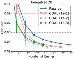
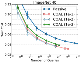
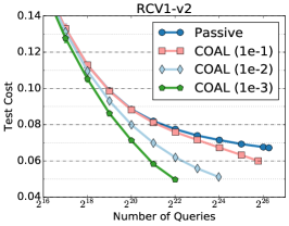
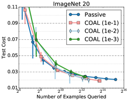
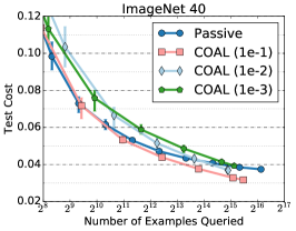
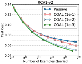
Figure 2: Experiments with COAL. Top row shows test cost vs. number of queries for simulated active learning experiments. Bottom row shows test cost vs. number of examples with even a single label query for simulated active learning experiments.

	$K$	$n$	feat	density
ImageNet 20	20	38k	6k	21.1%
ImageNet 40	40	71k	6k	21.0%
RCV1-v2	103	781k	47k	0.16%

	$K$	$n$	feat	$len$
POS	45	38k	40k	24
NER	9	15k	15k	14
Wiki	9	132k	89k	25

Table 1: Dataset statistics. $len$ is the average sequence length and density is the percentage of non-zero features.

We compare our online version of COAL to passive online learning. We use the cost-sensitive one-against-all (csoaa) implementation in Vowpal Wabbit, which performs online linear regression for each label separately. There are two tuning parameters in our implementation. First, instead of $\Delta_{i}$, we set the radius of the version space to $\Delta_{i}^{\prime}=\frac{\kappa\nu_{i-1}}{i-1}$ (i.e. the $\log(n)$ term in the definition of $\nu_{n}$ is replaced with $\log(i)$) and instead tune the constant $\kappa$. This alternate “mellowness" parameter controls how aggressive the query strategy is. The second parameter is the learning rate used by online linear regression.

For all experiments, we show the results obtained by the best learning rate for each mellowness on each dataset, which is tuned as follows. We randomly permute the training data 100 times and make one pass through the training set with each parameter setting. For each dataset let $\mathrm{perf}(mel,l,q,t)$ denote the test performance of the algorithm using mellowness $mel$ and learning rate $l$ on the $t^{\textrm{th}}$ permutation of the training data under a query budget of $2^{(q-1)}\cdot 10\cdot K,q\geq 1$. Let $\mathrm{query}(mel,l,q,t)$ denote the number of queries actually made. Note that $\mathrm{query}(mel,l,q,t)<2^{(q-1)}\cdot 10\cdot K$ if the algorithm runs out of the training data before reaching the $q^{\textrm{th}}$ query budget. To evaluate the trade-off between test performance and number of queries, we define the following performance measure:

$$\mathrm{AUC}(mel,l,t)=\frac{1}{2}\sum_{q=1}^{q_{\max}}\Big{(}\mathrm{perf}(mel,l,q+1,t)+\mathrm{perf}(mel,l,q,t)\Big{)}\cdot\log_{2}\frac{\mathrm{query}(mel,l,q+1,t)}{\mathrm{query}(mel,l,q,t)},$$ (14)

where $q_{\max}$ is the minimum $q$ such that $2^{(q-1)}\cdot 10$ is larger than the size of the training data. This performance measure is the area under the curve of test performance against number of queries in $\log_{2}$ scale. A large value means the test performance quickly improves with the number of queries. The best learning rate for mellowness $mel$ is then chosen as

$$l^{\star}(mel)\triangleq\arg\max_{l}\mathrm{median}_{1\leq t\leq 100}\quad\mathrm{AUC}(mel,l,t).$$

The best learning rates for different datasets and mellowness settings are in Table 2.

	ImageNet 20	ImageNet 40	RCV1-v2	POS	NER	NER-wiki
passive	1	1	0.5	1.0	0.5	0.5
active ($10^{-1}$)	0.05	0.1	0.5	1.0	0.1	0.5
active ($10^{-2}$)	0.05	0.5	0.5	1.0	0.5	0.5
active ($10^{-3}$)	1	10	0.5	10	0.5	0.5

Table 2: Best learning rates for each learning algorithm and each dataset.

In the top row of Figure 2, we plot, for each dataset and mellowness, the number of queries against the median test cost along with bars extending from the $15^{\textrm{th}}$ to $85^{\textrm{th}}$ quantile. Overall, COAL achieves a better trade-off between performance and queries. With proper mellowness parameter, active learning achieves similar test cost as passive learning with a factor of 8 to 32 fewer queries. On ImageNet 40 and RCV1-v2 (reproduced in Figure 1), active learning achieves better test cost with a factor of 16 fewer queries. On RCV1-v2, COAL queries like passive up to around $256k$ queries, since the data is very sparse, and linear regression has the property that the cost range is maximal when an example has a new unseen feature. Once COAL sees all features a few times, it queries much more efficiently than passive. These plots correspond to the label complexity $L_{2}$.

In the bottom row, we plot the test error as a function of the number of examples for which at least one query was requested, for each dataset and mellowness, which experimentally corresponds to the $L_{1}$ label complexity. In comparison to the top row, the improvements offered by active learning are slightly less dramatic here. This suggests that our algorithm queries just a few labels for each example, but does end up issuing at least one query on most of the examples. Nevertheless, one can still achieve test cost competitive with passive learning using a factor of 2-16 less labeling effort, as measured by $L_{1}$.

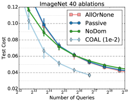
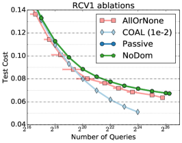
Figure 3: Test cost versus number of queries for COAL, in comparison with active and passive baselines on the ImageNet40 and RCV1-v2 dataset. On RCV1-v2, passive learning and NoDom are nearly identical.

We also compare COAL with two active learning baselines. Both algorithms differ from COAL only in their query rule. AllOrNone queries either all labels or no labels using both domination and cost-range conditions and is an adaptation of existing multiclass active learners [1]. NoDom just uses the cost-range condition, inspired by active regression [11]. The results for ImageNet 40 and RCV1-v2 are displayed in Figure 3, where we use the AUC strategy to choose the learning rate. We choose the mellowness by visual inspection for the baselines and use $0.01$ for COAL . On ImageNet 40, the ablations provide minimal improvement over passive learning, while on RCV1-v2, AllOrNone does provide marginal improvement. However, on both datasets, COAL substantially outperforms both baselines and passive learning.

While not always the best, we recommend a mellowness setting of $0.01$ as it achieves reasonable performance on all three datasets. This is also confirmed by the learning-to-search experiments, which we discuss next.

7.3 Learning to Search

We also experiment with COAL as the base leaner in learning-to-search [15, 13], which reduces joint prediction problems to CSMC. A joint prediction example defines a search space, where a sequence of decisions are made to generate the structured label. We focus here on sequence labeling tasks, where the input is a sentence and the output is a sequence of labels, specifically, parts of speech or named entities.

Learning-to-search solves such problems by generating the output one label at a time, conditioning on all past decisions. Since mistakes may lead to compounding errors, it is natural to represent the decision space as a CSMC problem, where the classes are the “actions” available (e.g., possible labels for a word) and the costs reflect the long term loss of each choice. Intuitively, we should be able to avoid expensive computation of long term loss on decisions like “is ‘the’ a determiner?” once we are quite sure of the answer. Similar ideas motivate adaptive sampling for structured prediction [40].

We specifically use Aggravate [37, 13, 42], which runs a learned policy to produce a backbone sequence of labels. For each position in the input, it then considers all possible deviation actions and executes an oracle for the rest of the sequence. The loss on this complete output is used as the cost for the deviating action. Run in this way, Aggravate requires $len\times K$ roll-outs when the input sentence has $len$ words and each word can take one of $K$ possible labels.

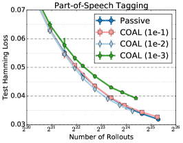
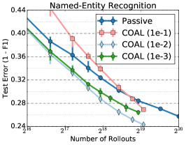
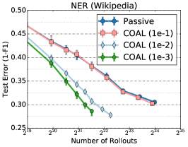
Figure 4: Learning to search experiments with COAL. Accuracy vs. number of rollouts for active and passive learning as the CSMC algorithm in learning-to-search.

Since each roll-out takes $\mathcal{O}(len)$ time, this can be computationally prohibitive, so we use active learning to reduce the number of roll-outs. We use COAL and a passive learning baseline inside Aggravate on three joint prediction datasets (statistics are in Table 1). As above, we use several mellowness values and the same AUC criteria to select the best learning rate (see Table 2). The results are in Figure 4, and again our recommended mellowness is $0.01$.

Overall, active learning reduces the number of roll-outs required, but the improvements vary on the three datasets. On the Wikipedia data, COAL performs a factor of 4 fewer rollouts to achieve similar performance to passive learning and achieves substantially better test performance. A similar, but less dramatic, behavior arises on the NER task. On the other hand, COAL offers minimal improvement over passive learning on the POS-tagging task. This agrees with our theory and prior empirical results [23], which show that active learning may not always improve upon passive learning.

8 Proofs

In this section we provide proofs for the main results, the oracle-complexity guarantee and the generalization and label complexity bounds. We start with some supporting results, including a new uniform freedman-type inequality that may be of independent interest. The proof of this inequality, and the proofs for several other supporting lemmata are deferred to the appendices.

8.1 Supporting Results

A deviation bound.

For both the computational and statistical analysis of COAL, we require concentration of the square loss functional $\widehat{R}_{j}(\cdot;y)$, uniformly over the class $\mathcal{G}$. To describe the result, we introduce the central random variable in the analysis:

$$M_{j}(g;y)\triangleq Q_{j}(y)\left[(g(x_{j})-c_{j}(y))^{2}-(f^{\star}(x_{j};y)-c_{j}(y))^{2}\right],$$ (15)

where $(x_{j},c_{j})$ is the $j^{\textrm{th}}$ example and cost presented to the algorithm and $Q_{j}(y)\in\{0,1\}$ is the query indicator. For simplicity we often write $M_{j}$ when the dependence on $g$ and $y$ is clear from context. Let $\mathbb{E}_{j}[\cdot]$ and $\operatorname*{{\rm Var}}_{j}[\cdot]$ denote the expectation and variance conditioned on all randomness up to and including round $j-1$.

Theorem 9.

Let $\mathcal{G}$ be a function class with $\mathrm{Pdim}(\mathcal{G})=d$, let $\delta\in(0,1)$ and define $\nu_{n}\triangleq 324(d\log(n)+\log(8Ke(d+1)n^{2}/\delta))$. Then with probability at least $1-\delta$, the following inequalities hold simultaneously for all $g\in\mathcal{G}$, $y\in[K]$, and $i<i^{\prime}\in[n]$.

$$\sum_{j=i}^{i^{\prime}}M_{j}(g;y) \leq\frac{3}{2}\sum_{j=i}^{i^{\prime}}\mathbb{E}_{j}M_{j}(g;y)+\nu_{n},$$ (16)

$$\frac{1}{2}\sum_{j=i}^{i^{\prime}}\mathbb{E}_{j}M_{j}(g;y) \leq\sum_{j=i}^{i^{\prime}}M_{j}(g;y)+\nu_{n}.$$ (17)

This result is a uniform Freedman-type inequality for the martingale difference sequence $\sum_{i}M_{i}-\mathbb{E}_{i}M_{i}$. In general, such bounds require much stronger assumptions (e.g., sequential complexity measures [35]) on $\mathcal{G}$ than the finite pseudo-dimension assumption that we make. However, by exploiting the structure of our particular martingale, specifically that the dependencies arise only from the query indicator, we are able to establish this type of inequality under weaker assumptions. The result may be of independent interest, but the proof, which is based on arguments from Liang et al. [29], is quite technical and deferred to Appendix A. Note that we did not optimize the constants.

The Multiplicative Weights Algorithm.

We also use the standard analysis of multiplicative weights for solving linear feasibility problems. We state the result here and, for completeness, provide a proof in Appendix B. See also Arora et al. [3], Plotkin et al. [34] for more details.

Consider a linear feasibility problem with decision variable $v\in\mathbb{R}^{d}$, explicit constraints $\langle a_{i},v\rangle\leq b_{i}$ for $i\in[m]$ and some implicit constraints $v\in S$ (e.g., $v$ is non-negative or other simple constraints). The MW algorithm either finds an approximately feasible point or certifies that the program is infeasible assuming access to an oracle that can solve a simpler feasibility problem with just one explicit constraint $\sum_{i}\mu_{i}\langle a_{i},v\rangle\leq\sum_{i}\mu_{i}b_{i}$ for any non-negative weights $\mu\in\mathbb{R}^{m}_{+}$ and the implicit constraint $v\in S$. Specifically, given weights $\mu$, the oracle either reports that the simpler problem is infeasible, or returns any feasible point $v$ that further satisfies $\langle a_{i},v\rangle-b_{i}\in[-\rho_{i},\rho_{i}]$ for parameters $\rho_{i}$ that are known to the MW algorithm.

The MW algorithm proceeds iteratively, maintaining a weight vector $\mu^{(t)}\in\mathbb{R}^{m}_{+}$ over the constraints. Starting with $\mu^{(1)}_{i}=1$ for all $i$, at each iteration, we query the oracle with the weights $\mu^{(t)}$ and the oracle either returns a point $v_{t}$ or detects infeasibility. In the latter case, we simply report infeasibility and in the former, we update the weights using the rule

$$\mu^{(t+1)}_{i}\leftarrow\mu^{(t)}_{i}\times\left(1-\eta\frac{b_{i}-\langle a_{i},v_{t}\rangle}{\rho_{i}}\right).$$

Here $\eta$ is a parameter of the algorithm. The intuition is that if $v_{t}$ satisfies the $i^{\textrm{th}}$ constraint, then we down-weight the constraint, and conversely, we up-weight every constraint that is violated. Running the algorithm with appropriate choice of $\eta$ and for enough iterations is guaranteed to approximately solve the feasibility problem.

Theorem 10 (Arora et al. [3], Plotkin et al. [34]).

Consider running the MW algorithm with parameter $\eta=\sqrt{\log(m)/T}$ for $T$ iterations on a linear feasibility problem where oracle responses satisfy $\langle a_{i},v\rangle-b_{i}\in[-\rho_{i},\rho_{i}]$. If the oracle fails to find a feasible point in some iteration, then the linear program is infeasible. Otherwise the point $\bar{v}\triangleq\frac{1}{T}\sum_{t=1}^{T}v_{t}$ satisfies $\langle a_{i},\bar{v}\rangle\leq b_{i}+2\rho_{i}\sqrt{\log(m)/T}$ for all $i\in[m]$.

Other Lemmata.

Our first lemma evaluates the conditional expectation and variance of $M_{j}$, defined in (15), which we will use heavily in the proofs. Proofs of the results stated here are deferred to Appendix C.

Lemma 2 (Bounding variance of regression regret).

We have for all $(g,y)\in\mathcal{G}\times\mathcal{Y}$,

$$\mathbb{E}_{j}[M_{j}]=\mathbb{E}_{j}\left[Q_{j}(y)(g(x_{j})-f^{\star}(x_{j};y))^{2}\right],\qquad\operatorname*{{\rm Var}}_{j}[M_{j}]\leq 4\mathbb{E}_{i}[M_{j}].$$

The next lemma relates the cost-sensitive error to the random variables $M_{j}$. Define

$$\mathcal{F}_{i}=\left\{f\in\mathcal{G}^{K}\mid\forall y,f(\cdot;y)\in\mathcal{G}_{i}(y)\right\},$$

which is the version space of vector regressors at round $i$. Additionally, recall that $P_{\zeta}$ captures the noise level in the problem, defined in (10) and that $\psi_{i}=1/\sqrt{i}$ is defined in the algorithm pseudocode.

Lemma 3.

For all $i>0$, if $f^{\star}\in\mathcal{F}_{i}$, then for all $f\in\mathcal{F}_{i}$

$$\mathbb{E}_{x,c}[c(h_{f}(x))-c(h_{{f}^{\star}}(x))]\leq\min_{\zeta>0}\left\{\zeta P_{\zeta}+\mathds{1}\left(\zeta\leq 2\psi_{i}\right)2\psi_{i}+\frac{4\psi_{i}^{2}}{\zeta}+\frac{6}{\zeta}\sum_{y}\mathbb{E}_{i}\left[M_{i}\right]\right\}.$$

Note that the lemma requires that both $f^{\star}$ and $f$ belong to the version space $\mathcal{F}_{i}$.

For the label complexity analysis, we will need to understand the cost-sensitive performance of all $f\in\mathcal{F}_{i}$, which requires a different generalization bound. Since the proof is similar to that of Theorem 3, we defer the argument to appendix.

Lemma 4.

Assuming the bounds in Theorem 9 hold, then for all $i$, $\mathcal{F}_{i}\subset\mathcal{F}_{\textrm{csr}}(r_{i})$ where $r_{i}\triangleq\min_{\zeta>0}\left\{\zeta P_{\zeta}+\frac{44K\Delta_{i}}{\zeta}\right\}.$

The final lemma relates the query rule of COAL to a hypothetical query strategy driven by $\mathcal{F}_{\textrm{csr}}(r_{i})$, which we will subsequently bound by the disagreement coefficients. Let us fix the round $i$ and introduce the shorthand $\widehat{\gamma}(x_{i},y)=\widehat{c}_{+}(x_{i},y)-\widehat{c}_{-}(x_{i},y)$, where $\widehat{c}_{+}(x_{i},y)$ and $\widehat{c}_{-}(x_{i},y)$ are the approximate maximum and minimum costs computed in Algorithm 1 on the $i^{\textrm{th}}$ example, which we now call $x_{i}$. Moreover, let $Y_{i}$ be the set of non-dominated labels at round $i$ of the algorithm, which in the pseudocode we call $Y^{\prime}$. Formally, $Y_{i}=\{y\mid\widehat{c}_{-}(x_{i},y)\leq\min_{y^{\prime}}\widehat{c}_{+}(x_{i},y^{\prime})\}$. Finally recall that for a set of vector regressors $F\subset\mathcal{F}$, we use $\gamma(x,y,F)$ to denote the cost range for label $y$ on example $x$ witnessed by the regressors in $F$.

Lemma 5.

Suppose that the conclusion of Lemma 4 holds. Then for any example $x_{i}$ and any label $y$ at round $i$, we have

$$\widehat{\gamma}(x_{i},y)\leq\gamma(x_{i},y,\mathcal{F}_{\textrm{csr}}(r_{i}))+\psi_{i}.$$

Further, with $y_{i}^{\star}=\mathop{\mathrm{argmin}}_{y}f^{\star}(x_{i};y),\bar{y}_{i}=\mathop{\mathrm{argmin}}_{y}\widehat{c}_{+}(x_{i},y)$, and $\tilde{y}_{i}=\mathop{\mathrm{argmin}}_{y\neq y_{i}^{\star}}\widehat{c}_{-}(x_{i},y)$,

$$y\neq y_{i}^{\star}\wedge y\in Y_{i} \Rightarrow f^{\star}(x_{i};y)-f^{\star}(x_{i};y_{i}^{\star})\leq\gamma(x_{i},y,\mathcal{F}_{\textrm{csr}}(r_{i}))+\gamma(x_{i},y_{i}^{\star},\mathcal{F}_{\textrm{csr}}(r_{i}))+\psi_{i}/2,$$

$$|Y_{i}|>1\wedge y_{i}^{\star}\in Y_{i} \Rightarrow f^{\star}(x_{i};\tilde{y}_{i})-f^{\star}(x_{i};y_{i}^{\star})\leq\gamma(x_{i},\tilde{y}_{i},\mathcal{F}_{\textrm{csr}}(r_{i}))+\gamma(x_{i},y_{i}^{\star},\mathcal{F}_{\textrm{csr}}(r_{i}))+\psi_{i}/2.$$

8.2 Proof of Theorem 1

The proof is based on expressing the optimization problem (7) as a linear optimization in the space of distributions over $\mathcal{G}$. Then, we use binary search to re-formulate this as a series of feasibility problems and apply Theorem 10 to each of these.

Recall that the problem of finding the maximum cost for an $(x,y)$ pair is equivalent to solving the program (7) in terms of the optimal $g$. For the problem (7), we further notice that since $\mathcal{G}$ is a convex set, we can instead write the minimization over $g$ as a minimization over $P\in\Delta(\mathcal{G})$ without changing the optimum, leading to the modified problem (8).

Thus we have a linear program in variable $P$, and Algorithm 2 turns this into a feasibility problem by guessing the optimal objective value and refining the guess using binary search. For each induced feasibility problem, we use MW to certify feasibility. Let $c\in[0,1]$ be some guessed upper bound on the objective, and let us first turn to the MW component of the algorithm. The program in consideration is

$$?\exists P\in\Delta(G)\textrm{ s.t. }\mathbb{E}_{g\sim P}(g(x_{i})-1)^{2}\leq c\textrm{ and }\forall j\in[i],\mathbb{E}_{g\sim P}\widehat{R}_{j}(g;y)\leq\tilde{\Delta}_{j}.$$ (18)

This is a linear feasibility problem in the infinite dimensional variable $P$, with $i+1$ constraints. Given a particular set of weights $\mu$ over the constraints, it is clear that we can use the regression oracle over $g$ to compute

$$g_{\mu}=\arg\min_{g\in\mathcal{G}}\mu_{0}(g(x_{i})-1)^{2}+\sum_{j\in[i]}\mu_{j}\mathbb{E}_{g\sim P}\widehat{R}_{j}(g;y).$$ (19)

Observe that solving this simpler program provides one-sided errors. Specifically, if the objective of (19) evaluated at $g_{\mu}$ is larger than $\mu_{0}c+\sum_{j\in[i]}\mu_{j}\tilde{\Delta}_{j}$ then there cannot be a feasible solution to problem (18), since the weights $\mu$ are all non-negative. On the other hand if $g_{\mu}$ has small objective value it does not imply that $g_{\mu}$ is feasible for the original constraints in (18).

At this point, we would like to invoke the MW algorithm, and specifically Theorem 10, in order to find a feasible solution to (18) or to certify infeasibility. Invoking the theorem requires the $\rho_{j}$ parameters which specify how badly $g_{\mu}$ might violate the $j^{\textrm{th}}$ constraint. For us, $\rho_{j}\triangleq\kappa$ suffices since $\hat{R}_{j}(g;y)-\hat{R}_{j}(g_{j,y};y)\in[0,1]$ (since $g_{j,y}$ is the ERM) and $\Delta_{j}\leq\kappa$. Since $\kappa\geq 2$ this also suffices for the cost constraint.

If at any iteration, MW detects infeasibility, then our guessed value $c$ for the objective is too small since no function satisfies both $(g(x_{i})-1)^{2}\leq c$ and the empirical risk constraints in (18) simultaneously. In this case, in Line 10 of Algorithm 2, our binary search procedure increases our guess for $c$. On the other hand, if we apply MW for $T$ iterations and find a feasible point in every round, then, while we do not have a point that is feasible for the original constraints in (18), we will have a distribution $P_{T}$ such that

$$\mathbb{E}_{P_{T}}(g(x_{i})-1)^{2}\leq c+2\kappa\sqrt{\frac{\log(i+1)}{T}}\textrm{ and }\forall j\in[i],\mathbb{E}_{P_{T}}\widehat{R}_{j}(g;y)\leq\tilde{\Delta}_{j}+2\kappa\sqrt{\frac{\log(i+1)}{T}}.$$

We will set $T$ toward the end of the proof.

If we do find an approximately feasible solution, then we reduce $c$ and proceed with the binary search. We terminate when $c_{h}-c_{\ell}\leq\tau^{2}/2$ and we know that problem (18) is approximately feasible with $c_{h}$ and infeasible with $c_{\ell}$. From $c_{h}$ we will construct a strictly feasible point, and this will lead to a bound on the true maximum $c_{+}(x,y,\mathcal{G}_{i})$.

Let $\bar{P}$ be the approximately feasible point found when running MW with the final value of $c_{h}$. By Jensen’s inequality and convexity of $\mathcal{G}$, there exists a single regressor that is also approximately feasible, which we denote $\bar{g}$. Observe that $g^{\star}$ satisfies all constraints with strict inequality, since by (20) we know that $\widehat{R}_{j}(g^{\star};y)-\widehat{R}_{j}(g_{j,y};y)\leq\Delta_{j}/\kappa<\Delta_{j}$. We create a strictly feasible point $g_{\zeta}$ by mixing $\bar{g}$ with $g^{\star}$ with proportion $1-\zeta$ and $\zeta$ for

$$\zeta=\frac{4\kappa}{\Delta_{i}}\sqrt{\frac{\log(i+1)}{T}},$$

which will be in $[0,1]$ when we set $T$. Combining inequalities, we get that for any $j\in[i]$

$$(1-\zeta)\widehat{R}_{j}(\bar{g};y)+\zeta\widehat{R}_{j}(g^{\star};y) \leq\widehat{R}_{j}(g_{j,y};y)+(1-\zeta)\left(\Delta_{j}+2\kappa\sqrt{\frac{\log(i+1)}{T}}\right)+\zeta\left(\frac{\Delta_{j}}{\kappa}\right)$$

$$\leq\widehat{R}_{j}(g_{j,y};y)+\Delta_{j}-\left(\frac{\zeta\Delta_{j}(\kappa-1)}{\kappa}-2\kappa\sqrt{\frac{\log(i+1)}{T}}\right)$$

$$\leq\widehat{R}_{j}(g_{j,y};y)+\Delta_{j},$$

and hence this mixture regressor $g_{\zeta}$ is exactly feasible. Here we use that $\kappa\geq 2$ and that $\Delta_{i}$ is monotonically decreasing. With the pessimistic choice $g^{\star}(x_{i})=0$, the objective value for $g_{\zeta}$ is at most

$$(g_{\zeta}(x_{i})-1)^{2} \leq(1-\zeta)(\bar{g}(x_{i})-1)^{2}+\zeta(g^{\star}(x_{i})-1)^{2}\leq(1-\zeta)\left(c_{h}+2\kappa\sqrt{\frac{\log(i+1)}{T}}\right)+\zeta$$

$$\leq c_{\ell}+\tau^{2}/2+\left(2\kappa+\frac{4\kappa}{\Delta_{i}}\right)\sqrt{\frac{\log(i+1)}{T}}.$$

Thus $g_{\zeta}$ is exactly feasible and achieves the objective value above, which provides an upper bound on the maximum cost. On the other hand $c_{\ell}$ provides a lower bound. Our setting of $T=\frac{\log(i+1)(8\kappa^{2}/\Delta_{i})^{2}}{\tau^{4}}$ ensures that that this excess term is at most $\tau^{2}$, since $\Delta_{i}\leq 1$. Note that since $\tau\leq[0,1]$, this also ensures that $\zeta\in[0,1]$. With this choice of $T$, we know that $c_{\ell}\leq(c_{+}(y)-1)^{2}\leq c_{\ell}+\tau^{2}$, which implies that $c_{+}(y)\in[1-\sqrt{c_{\ell}+\tau^{2}},1-\sqrt{c_{\ell}}]$. Since $\sqrt{c_{\ell}+\tau^{2}}\leq\sqrt{c_{\ell}}+\tau$, we obtain the guarantee.

As for the oracle complexity, since we start with $c_{\ell}=0$ and $c_{h}=1$ and terminate when $c_{h}-c_{\ell}\leq\tau^{2}/2$, we perform $\mathcal{O}(\log(1/\tau^{2}))$ iterations of binary search. Each iteration requires $T=\mathcal{O}\left(\max\{1,i^{2}/\nu_{n}^{2}\}\frac{\log(i)}{\tau^{4}}\right)$ rounds of MW, each of which requires exactly one oracle call. Hence the oracle complexity is $\mathcal{O}\left(\max\{1,i^{2}/\nu_{n}^{2}\}\frac{\log(i)\log(1/\tau)}{\tau^{4}}\right)$.

8.3 Proof of the Generalization Bound

Recall the central random variable $M_{j}(g;y)$, defined in (15), which is the excess square loss for function $g$ on label $y$ for the $j^{\textrm{th}}$ example, if we issued a query. The idea behind the proof is to first apply Theorem 9 to argue that all the random variables $M_{j}(g;y)$ concentrate uniformly over the function class $\mathcal{G}$. Next for a vector regressor $f$, we relate the cost-sensitive risk to the excess square loss via Lemma 3. Finally, using the fact that $g_{i,y}$ minimizes the empirical square loss at round $i$, this implies a cost-sensitive risk bound for the vector regressor $f_{i}=(g_{i,y})$ at round $i$.

First, condition on the high probability event in Theorem 9, which ensures that the empirical square losses concentrate. We first prove that $f^{\star}\in\mathcal{F}_{i}$ for all $i\in[n]$. At round $i$, by (17), for each $y$ and for any $g$ we have

$$0\leq\frac{1}{2}\sum_{j=1}^{i}\mathbb{E}_{j}M_{j}(g;y)\leq\sum_{j=1}^{i}M_{j}(g;y)+\nu_{n}.$$

The first inequality here follows from the fact that $\mathbb{E}_{j}M_{j}(g;y)$ is a quadratic form by Lemma 2. Expanding $M_{j}(g;y)$, this implies that

$$\widehat{R}_{i+1}(f^{\star}(\cdot;y);y)\leq\widehat{R}_{i+1}(g;y)+\frac{\nu_{n}}{i}.$$

Since this bound applies to all $g\in\mathcal{G}$ it proves that $f^{\star}\in\mathcal{F}_{i+1}$ for all $i$, using the definition of $\Delta_{i}$ and $\kappa$. Trivially, we know that $f^{\star}\in\mathcal{F}_{1}$. Together with the fact that the losses are in $[0,1]$ and the definition of $\Delta_{i}$, the above analysis yields

$$\widehat{R}_{i}(f^{\star}(\cdot;y);y)\leq\widehat{R}_{i}(g;y)+\frac{\Delta_{i}}{\kappa}.$$ (20)

This implies that $f^{\star}(\cdot;y)$ strictly satisfies the inequalities defining the version space, which we used in the MW proof.

We next prove that $f_{i+1}\in\mathcal{F}_{j}$ for all $j\in[i]$. Fix some label $y$ and to simplify notation, we drop dependence on $y$. If $g_{i+1}\notin\mathcal{G}_{t+1}$ for some $t\in\{0,\ldots,i\}$ then, first observe that we must have $t$ large enough so that $\nu_{n}/t\leq 1$. In particular, since $\Delta_{t+1}=\kappa\min\{1,\nu_{n}/t\}$ and we always have $\hat{R}_{t+1}(g_{i+1};y)\leq\hat{R}_{t+1}(g_{t+1};y)+1$ due to boundedness, we do not evict any functions until $\nu_{n}/t\leq 1$. For $t\geq\nu_{n}$, we get

$$\sum_{j=1}^{t}M_{j} =t\left(\widehat{R}_{t+1}(g_{i+1})-\widehat{R}_{t+1}(g^{\star})\right)$$

$$=t\left(\widehat{R}_{t+1}(g_{i+1})-\widehat{R}_{t+1}(g_{t+1})+\widehat{R}_{t+1}(g_{t+1})-\widehat{R}_{t+1}(g^{\star})\right)$$

$$\geq\kappa\nu_{n}-\nu_{n}=(\kappa-1)\nu_{n}.$$

The inequality uses the radius of the version space and the fact that by assumption $g_{i+1}\notin\mathcal{G}_{t+1}$, so the excess empirical risk is at least $\Delta_{t+1}=\kappa\nu_{n}/t$ since we are considering large $t$. We also use (20) on the second term. Moreover, we know that since $g_{i+1}$ is the empirical square loss minimizer for label $y$ after round $i$, we have $\sum_{j=1}^{i}M_{j}(g_{i+1};y)\leq 0$. These two facts together establish that

$$\sum_{j=t+1}^{i}M_{j}(g_{i+1})\leq(1-\kappa)\nu_{n}.$$

However, by Theorem 9 on this intermediary sum, we know that

$$0\leq\frac{1}{2}\sum_{j=t+1}^{i}\mathbb{E}_{j}M_{j}(g_{i+1})\leq\sum_{j=t+1}^{i}M_{j}(g_{i+1})+\nu_{n}<(2-\kappa)\nu_{n}<0$$

using the definition of $\kappa$. This is a contradiction, so we must have that $g_{i+1}\in\mathcal{G}_{j}$ for all $j\in\{1,\ldots,i\}$. The same argument applies for all $y$ and hence we can apply Lemma 3 on all rounds to obtain

$$i\big{(}\mathbb{E}_{x,c}[c(h_{f_{i+1}}(x))-c(h_{f^{\star}}(x))]\big{)}$$

$$\leq\min_{\zeta>0}\left\{i\zeta P_{\zeta}+\sum_{j=1}^{i}\left(\mathds{1}\left(\zeta\leq 2\psi_{j}\right)2\psi_{j}+\frac{4\psi_{j}^{2}}{\zeta}+\frac{6}{\zeta}\sum_{y}\mathbb{E}_{j}\left[M_{j}(f_{i+1};y)\right]\right)\right\}.$$

We study the four terms separately. The first one is straightforward and contributes $\zeta P_{\zeta}$ to the instantaneous cost sensitive regret. Using our definition of $\psi_{j}=1/\sqrt{j}$ the second term can be bounded as

$$\sum_{j=1}^{i}\mathds{1}\left(\zeta<2\psi_{j}\right)2\psi_{j} =\sum_{j=1}^{\lceil 4/\zeta^{2}\rceil}\frac{2}{\sqrt{j}}\leq 4\sqrt{\lceil 4/\zeta^{2}\rceil}\leq\frac{12}{\zeta}.$$

The inequality above, $\sum_{i=1}^{n}\frac{1}{\sqrt{i}}\leq 2\sqrt{n}$, is well known. For the third term, using our definition of $\psi_{j}$ gives

$$\sum_{j=1}^{i}\frac{4\psi_{j}^{2}}{\zeta}=\frac{4}{\zeta}\sum_{j=1}^{i}\frac{1}{j}\leq\frac{4}{\zeta}(1+\log(i)).$$

Finally, the fourth term can be bounded using (17), which reveals

$$\sum_{j=1}^{i}\mathbb{E}_{j}[M_{j}]\leq 2\sum_{j=1}^{i}M_{j}+2\nu_{n}$$

Since for each $y$, $\sum_{j=1}^{i}M_{j}(f_{i+1};y)\leq 0$ for the empirical square loss minimizer (which is what we are considering now), we get

$$\frac{6}{\zeta}\sum_{y}\sum_{j=1}^{i}\mathbb{E}_{j}[M_{j}(f_{i+1};y)]\leq\frac{12}{\zeta}K\nu_{n}.$$

And hence, we obtain the generalization bound

$$\mathbb{E}_{x,c}[c(x;h_{f_{i+1}}(x))-c(x;h_{f^{\star}}(x))] \leq\min_{\zeta>0}\left\{\zeta P_{\zeta}+\frac{1}{\zeta i}\left(4\log(i)+16+12K\nu_{n}\right)\right\}$$

$$\leq\min_{\zeta>0}\left\{\zeta P_{\zeta}+\frac{32K\nu_{n}}{\zeta i}\right\}.$$

Proof of Corollary 4.

Under the Massart noise condition, set $\zeta=\tau$ so that $P_{\zeta}=0$ and we immediately get the result.

Proof of Corollary 5.

Set $\zeta=\min\left\{\tau_{0},\left(\frac{32K\nu_{n}}{i\beta}\right)^{\frac{1}{\alpha+2}}\right\}$, so that for $i$ sufficiently large the second term is selected and we obtain the bound.

8.4 Proof of the Label Complexity bounds

The proof for the label complexity bounds is based on first relating the version space $\mathcal{F}_{i}$ at round $i$ to the cost-sensitive regret ball $\mathcal{F}_{\textrm{csr}}$ with radius $r_{i}$. In particular, the containment $\mathcal{F}_{i}\subset\mathcal{F}_{\textrm{csr}}(r_{i})$ in Lemma 4 implies that our query strategy is more aggressive than the query strategy induced by $\mathcal{F}_{\textrm{csr}}(r_{i})$, except for a small error introduced when computing the maximum and minimum costs. This error is accounted for by Lemma 5. Since the probability that $\mathcal{F}_{\textrm{csr}}$ will issue a query is intimately related to the disagreement coefficient, this argument leads to the label complexity bounds for our algorithm.

Proof of Theorem 6.

Fix some round $i$ with example $x_{i}$, let $\mathcal{F}_{i}$ be the vector regressors used at round $i$ and let $\mathcal{G}_{i}(y)$ be the corresponding regressors for label $y$. Let $\bar{y}_{i}=\mathop{\mathrm{argmin}}_{y}\widehat{c_{+}}(x_{i},y),y_{i}^{\star}=\mathop{\mathrm{argmin}}_{y}f^{\star}(x_{i};y)$, and $\tilde{y}_{i}=\mathop{\mathrm{argmin}}_{y\neq y_{i}^{\star}}\widehat{c_{-}}(x_{i},y)$. Assume that Lemma 4 holds. The $L_{2}$ label complexity is

$$\sum_{y}Q_{i}(y) =\sum_{y}{\bf 1}\{|Y_{i}|>1\wedge y\in Y_{i}\}{\bf 1}\{\widehat{\gamma}(x_{i},y)>\psi_{i}\}$$

$$\leq\sum_{y}{\bf 1}\{|Y_{i}|>1\wedge y\in Y_{i}\}{\bf 1}\{\gamma(x_{i},y,\mathcal{F}_{\textrm{csr}}(r_{i}))>\psi_{i}/2\}.$$

For the former indicator, observe that $y\in Y_{i}$ implies that there exists a vector regressor $f\in\mathcal{F}_{i}\subset\mathcal{F}_{\textrm{csr}}(r_{i})$ such that $h_{f}(x_{i})=y$. This follows since the domination condition means that there exists $g\in\mathcal{G}_{i}(y)$ such that $g(x_{i})\leq\min_{y^{\prime}}\max_{g^{\prime}\in\mathcal{G}_{i}(y^{\prime})}g^{\prime}(x_{i})$. Since we are using a factored representation, we can take $f$ to use $g$ on the $y^{\textrm{th}}$ coordinate and use the maximizers for all the other coordinates. Similarly, there exists another regressor $f^{\prime}\in\mathcal{F}_{i}$ such that $h_{f^{\prime}}(x_{i})\neq y$. Thus this indicator can be bounded by the disagreement coefficient

$$\sum_{y}Q_{i}(y) \leq\sum_{y}{\bf 1}\{\exists f,f^{\prime}\in\mathcal{F}_{\textrm{csr}}(r_{i})\mid h_{f}(x_{i})=y\neq h_{f^{\prime}}(x_{i})\}{\bf 1}\{\gamma(x_{i},y,\mathcal{F}_{\textrm{csr}}(r_{i}))>\psi_{i}/2\}$$

$$=\sum_{y}{\bf 1}\{x\in\textrm{DIS}(r_{i},y)\wedge\gamma(x_{i},y,\mathcal{F}_{\textrm{csr}}(r_{i}))\geq\psi_{i}/2\}.$$

We will now apply Freedman’s inequality on the sequence $\{\sum_{y}Q_{i}(y)\}_{i=1}^{n}$, which is a martingale with range $K$. Moreover, due to non-negativity, the conditional variance is at most $K$ times the conditional mean, and in such cases, Freedman’s inequality reveals that with probability at least $1-\delta$

$$X\leq\mathbb{E}X+2\sqrt{R\mathbb{E}X\log(1/\delta)}+2R\log(1/\delta)\leq 2\mathbb{E}X+3R\log(1/\delta),$$

where $X$ is the non-negative martingale with range $R$ and expectation $\mathbb{E}X$. The last step is by the fact that $2\sqrt{ab}\leq a+b$.

For us, Freedman’s inequality implies that with probability at least $1-\delta/2$

$$\sum_{i=1}^{n}\sum_{y}Q_{i}(y) \leq 2\sum_{i}\mathbb{E}_{i}\sum_{y}Q_{i}(y)+3K\log(2/\delta)$$

$$\leq 2\sum_{i}\mathbb{E}_{i}\sum_{y}{\bf 1}\{x\in\textrm{DIS}(r_{i},y)\wedge\gamma(x_{i},y,\mathcal{F}_{\textrm{csr}}(r_{i}))\geq\psi_{i}/2\}+3K\log(2/\delta)$$

$$\leq 4\sum_{i}\frac{r_{i}}{\psi_{i}}\theta_{2}+3K\log(2/\delta).$$

The last step here uses the definition of the disagreement coefficient $\theta_{2}$. To wrap up the proof we just need to upper bound the sequence, using our choices of $\psi_{i}=1/\sqrt{i}$, $r_{i}=2\sqrt{44K\Delta_{i}}$, and $\Delta_{i}=\kappa\min\{1,\frac{\nu_{n}}{i-1}\}$. With simple calculations this is easily seen to be at most

$$8n\theta_{2}\sqrt{88K\kappa\nu_{n}}+3K\log(2/\delta).$$

Similarly for $L_{1}$ we can derive the bound

$$L_{1}\leq\sum_{i}\mathds{1}\left(\exists y\mid\gamma(x_{i},y,\mathcal{F}_{\textrm{csr}}(r_{i}))\geq\psi_{i}/2\wedge x\in\textrm{DIS}(r_{i},y)\right),$$

and then apply Freedman’s inequality to obtain that with probability at least $1-\delta/2$

$$L_{1} \leq 2\sum_{i=1}^{n}\frac{2r_{i}}{\psi_{i}}\theta_{1}+3\log(2/\delta)\leq 8\theta_{1}n\sqrt{88K\kappa\nu_{n}}+3\log(2/\delta).$$

Proof of Theorem 7.

Using the same notations as in the bound for the high noise case we first express the $L_{2}$ label complexity as

$$\sum_{y}Q_{i}(y) =\sum_{y}{\bf 1}\{|Y_{i}|>1,y\in Y_{i}\}Q_{i}(y).$$

We need to do two things with the first part of the query indicator, so we have duplicated it here. For the second, we will use the derivation above to relate the query rule to the disagreement region. For the first, by Lemma 5, for $y\neq y_{i}^{\star}$, we can derive the bound

$${\bf 1}\{f^{\star}(x_{i};y)-f^{\star}(x_{i};y_{i}^{\star})\leq\gamma(x_{i},y,\mathcal{F}_{\textrm{csr}}(r_{i}))+\gamma(x_{i},y_{i}^{\star},\mathcal{F}_{\textrm{csr}}(r_{i}))+\psi_{i}/2\}$$

$$\leq{\bf 1}\{\tau-\psi_{i}/2\leq\gamma(x_{i},y,\mathcal{F}_{\textrm{csr}}(r_{i}))+\gamma(x_{i},y_{i}^{\star},\mathcal{F}_{\textrm{csr}}(r_{i}))\}.$$

For $y=y_{i}^{\star}$, we get the same bound but with $\tilde{y}_{i}$, also by Lemma 5. Focusing on just one of these terms, say where $y\neq y_{i}^{\star}$ and any round where $\tau\geq\psi_{i}$, we get

$${\bf 1}\{\tau-\psi_{i}/2\leq\gamma(x_{i},y,\mathcal{F}_{\textrm{csr}}(r_{i}))+\gamma(x_{i},y_{i}^{\star},\mathcal{F}_{\textrm{csr}}(r_{i}))\}Q_{i}(y)$$

$$\leq{\bf 1}\{\tau/2\leq\gamma(x_{i},y,\mathcal{F}_{\textrm{csr}}(r_{i}))+\gamma(x_{i},y_{i}^{\star},\mathcal{F}_{\textrm{csr}}(r_{i}))\}Q_{i}(y)$$

$$\leq{\bf 1}\{\tau/4\leq\gamma(x_{i},y,\mathcal{F}_{\textrm{csr}}(r_{i}))\}Q_{i}(y)+{\bf 1}\{\tau/4\leq\gamma(x_{i},y_{i}^{\star},\mathcal{F}_{\textrm{csr}}(r_{i}))\}Q_{i}(y)$$

$$\leq D_{i}(y)+D_{i}(y_{i}^{\star}),$$

where for shorthand we have defined $D_{i}(y)\triangleq{\bf 1}\{\tau/4\leq\gamma(x_{i},y,\mathcal{F}_{\textrm{csr}}(r_{i}))\wedge x_{i}\in\textrm{DIS}(r_{i},y)\}$. The derivation for the first term is straightforward. We obtain the disagreement region for $y_{i}^{\star}$ since the fact that we query $y$ (i.e. $Q_{i}(y)$) implies there is $f$ such that $h_{f}(x_{i})=y$, so this function witnesses disagreement to $y_{i}^{\star}$.

The term involving $y_{i}^{\star}$ and $\tilde{y}_{i}$ is bounded in essentially the same way, since we know that when $|Y_{i}|>1$, there exists two function $f,f^{\prime}\in\mathcal{F}_{i}$ such that $h_{f}(x_{i})=\tilde{y}_{i}$ and $h_{f^{\prime}}(x_{i})=y_{i}^{\star}$. In total, we can bound the $L_{2}$ label complexity at any round $i$ such that $\tau\geq\psi_{i}$ by

$$L_{2}\leq D_{i}(\tilde{y}_{i})+D_{i}(y_{i}^{\star})+\sum_{y\neq y_{i}^{\star}}\left(D_{i}(y)+D_{i}(y_{i}^{\star})\right)\leq KD_{i}(y_{i}^{\star})+2\sum_{y}D_{i}(y)$$

For the earlier rounds, we simply upper bound the label complexity by $K$. Since the range of this random variable is at most $3K$, using Freedman’s inequality just as in the high noise case, we get that with probability at least $1-\delta/2$

$$L_{2} \leq\sum_{i=1}^{n}K{\bf 1}\{\tau\leq\psi_{i}\}+2\sum_{i=2}^{n}\mathbb{E}_{i}\left[KD_{i}(y_{i}^{\star})+2\sum_{y}D_{i}(y)\right]+9K\log(2/\delta)$$

$$\leq K\lceil 1/\tau^{2}\rceil+\frac{8}{\tau}(K\theta_{1}+\theta_{2})\sum_{i=2}^{n}r_{i}+9K\log(2/\delta).$$

The first line here is the application of Freedman’s inequality. In the second, we evaluate the expectation, which we can relate to the disagreement coefficients $\theta_{1},\theta_{2}$. Moreover, we use the setting $\psi_{i}=1/\sqrt{i}$ to evaluate the first term. As a technicality, we remove the index $i=1$ from the second summation, since we are already accounting for queries on the first round in the first term. The last step is to evaluate the series, for which we use the definition of $r_{i}=\min_{\zeta>0}\left\{\zeta P_{\zeta}+44K\Delta_{i}/\zeta\right\}$ and set $\zeta=\tau$, the Massart noise level. This gives $r_{i}=44K\Delta_{i}/\tau$. In total, we get

$$L_{2}\leq K\lceil 1/\tau^{2}\rceil+\frac{352K\kappa\nu_{n}}{\tau^{2}}(K\theta_{1}+\theta_{2})\log(n)+9K\log(2/\delta).$$

As $\theta_{2}\leq K\theta_{1}$ always, we drop $\theta_{2}$ from the above expression to obtain the stated bound.

For $L_{1}$ we use a very similar argument. First, by Lemmas 4 and 5

$$L_{1}\leq\sum_{i=1}^{n}{\bf 1}\{|Y_{i}|>1\wedge\exists y\in Y_{i},\gamma(x_{i},y,\mathcal{F}_{\textrm{csr}}(r_{i}))\geq\psi_{i}/2\}.$$

Again by Lemma 5, we know that

$$|Y_{i}|>1\wedge y\in Y_{i}\Rightarrow\exists f,f^{\prime}\in\mathcal{F}_{\textrm{csr}}(r_{i}),h_{f}(x_{i})=y\neq h_{f^{\prime}}(x_{i}).$$

Moreover, one of the two classifiers can be $f^{\star}$, and so, when $\tau\geq\psi_{i}$, we can deduce

$$\Rightarrow f^{\star}(x_{i},y)-f^{\star}(x_{i},y_{i}^{\star})\leq\gamma(x_{i},y,\mathcal{F}_{\textrm{csr}}(r_{i}))+\gamma(x_{i},y_{i}^{\star},\mathcal{F}_{\textrm{csr}}(r_{i}))+\psi_{i}/2$$

$$\Rightarrow\tau/4\leq\gamma(x_{i},y,\mathcal{F}_{\textrm{csr}}(r_{i}))\wedge\tau/4\leq\gamma(x_{i},y_{i}^{\star},\mathcal{F}_{\textrm{csr}}(r_{i})).$$

Combining this argument, we bound the $L_{1}$ label complexity as

$$L_{1}\leq\sum_{i=1}^{n}{\bf 1}\{\tau\leq\psi_{i}\}+\sum_{i=2}^{n}{\bf 1}\{\exists y\mid x_{i}\in\textrm{DIS}(\mathcal{F}_{\textrm{csr}}(r_{i}),y)\wedge\gamma(x_{i},y,\mathcal{F}_{\textrm{csr}}(r_{i}))\geq\tau/4\}.$$ (21)

Applying Freedman’s inequality just as before gives

$$L_{1} \leq\lceil 1/\tau^{2}\rceil+2\sum_{i=2}^{n}\frac{4r_{i}}{\tau}\theta_{1}+2\log(2/\delta)\leq\lceil 1/\tau^{2}\rceil+\frac{352K\kappa\nu_{n}}{\tau^{2}}\theta_{1}\log(n)+2\log(2/\delta),$$

with probability at least $1-\delta/2$.

Proof of Theorem 8.

For the Tsybakov case, the same argument as in the Massart case gives that with probability at least $1-\delta/2$

$$L_{2}\leq K\lceil 1/\tau^{2}\rceil+\frac{8}{\tau}(K\theta_{1}+\theta_{2})\sum_{i=2}^{n}r_{i}+2n\beta\tau^{\alpha}+9K\log(2/\delta).$$

The main difference here is the term scaling with $n\tau^{\alpha}$ which arises since we do not have the deterministic bound $f^{\star}(x_{i},y)-f^{\star}(x_{i},y_{i}^{\star})\geq\tau$ as we used in the Massart case, but rather this happens except with probability $\beta\tau^{\alpha}$ (provided $\tau\leq\tau_{0}$). Now we must optimize $\zeta$ in the definition of $r_{i}$ and then $\tau$.

For $\zeta$ the optimal setting is $(44K\Delta_{i}/\beta)^{\frac{1}{\alpha+2}}$ which gives $r_{i}\leq 2\beta^{\frac{1}{\alpha+2}}(44K\Delta_{i})^{\frac{\alpha+1}{\alpha+2}}$. Since we want to set $\zeta\leq\tau_{0}$, this requires $i\geq 1+\frac{44K\kappa\nu_{n}}{\beta\tau_{0}^{\alpha+2}}$. For these early rounds we will simply pay $K$ in the label complexity, but this will be dominated by other higher order terms. For the later rounds, we get

$$\sum_{i=2}^{n}r_{i}\leq 2\beta^{\frac{1}{\alpha+2}}\left(44K\kappa\nu_{n}\right)^{\frac{\alpha+1}{\alpha+2}}\sum_{i=2}^{n}\left(\frac{1}{i-1}\right)^{\frac{\alpha+1}{\alpha+2}}\leq 2(\alpha+2)\left(44K\kappa\nu_{n}\right)^{\frac{\alpha+1}{\alpha+2}}(\beta n)^{\frac{1}{\alpha+2}}.$$

This bound uses the integral approximation $\sum_{i=2}^{n}(i-1)^{-\frac{\alpha+1}{\alpha+2}}\leq 1+\int_{1}^{n-1}x^{-\frac{\alpha+1}{\alpha+2}}dx\leq(\alpha+2)n^{\frac{1}{\alpha+2}}$. At this point, the terms involving $\tau$ in our bound are

$$K\lceil 1/\tau^{2}\rceil+\frac{16}{\tau}(K\theta_{1}+\theta_{2})(\alpha+2)\left(44K\kappa\nu_{n}\right)^{\frac{\alpha+1}{\alpha+2}}(\beta n)^{\frac{1}{\alpha+2}}+2n\beta\tau^{\alpha}.$$

We set $\tau=(8(\alpha+2)(K\theta_{1}+\theta_{2}))^{\frac{1}{\alpha+1}}\left(44K\kappa\nu_{n}\right)^{\frac{1}{\alpha+2}}(\beta n)^{\frac{-1}{\alpha+2}}$ by optimizing the second two terms which gives a final bound of

$$L_{2}\leq\mathcal{O}\left((K\theta_{1}+\theta_{2})^{\frac{\alpha}{\alpha+1}}(K\nu_{n})^{\frac{\alpha}{\alpha+2}}n^{\frac{2}{\alpha+2}}+K\log(1/\delta)\right).$$

This follows since the $1/\tau^{2}$ term agrees in the $n$ dependence and is lower order in other parameters, while the unaccounted for querying in the early rounds is independent of $n$. The bound of course requires that $\tau\leq\tau_{0}$, which again requires $n$ large enough. Note we are treating $\alpha$ and $\beta$ as constants and we drop $\theta_{2}$ from the final statement.

The $L_{1}$ bound requires only slightly different calculations. Following the derivation for the Massart case, we get

$$L_{1} \leq\lceil 1/\tau^{2}\rceil+\frac{8\theta_{1}}{\tau}\sum_{i=2}^{n}r_{i}+2n\beta\tau^{\alpha}+2\log(2/\delta)$$

$$\leq\lceil 1/\tau^{2}\rceil+\frac{16\theta_{1}(\alpha+2)}{\tau}\left(44K\kappa\nu_{n}\right)^{\frac{\alpha+1}{\alpha+2}}(\beta n)^{\frac{1}{\alpha+2}}+2n\beta\tau^{\alpha}+2\log(2/\delta),$$

not counting the lower order term for the querying in the early rounds. Here we set $\tau=(8(\alpha+2)\theta_{1})^{\frac{1}{\alpha+1}}\left(44K\kappa\nu_{n}\right)^{\frac{1}{\alpha+2}}(\beta n)^{\frac{-1}{\alpha+2}}$ to obtain

$$L_{1}\leq\mathcal{O}\left(\theta_{1}^{\frac{\alpha}{\alpha+1}}(K\nu_{n})^{\frac{\alpha}{\alpha+2}}n^{\frac{2}{\alpha+2}}+\log(1/\delta)\right).$$

Proof of Proposition 1: Massart Case.

Observe that with Massart noise, we have $\mathcal{F}_{\textrm{csr}}(r)\subset\widetilde{\mathcal{F}}(r/\tau)$, which implies that

$$\mathbb{E}{\bf 1}\left\{\exists y\mid x\in\textrm{DIS}(r,y)\wedge\gamma(x,y,\mathcal{F}_{\textrm{csr}}(r))\geq\tau/4\right\} \leq\mathbb{E}{\bf 1}\left\{x\in\widetilde{\textrm{DIS}}(r/\tau)\right\}$$

$$\leq\frac{r}{\tau}\sup_{r>0}\frac{1}{r}\mathbb{E}{\bf 1}\left\{x\in\widetilde{\textrm{DIS}}(r)\right\}.$$

Thus we may replace $\theta_{1}$ with $\theta_{0}$ in the proof of the $L_{1}$ label complexity bound above.

Proof of Proposition 1: Tsybakov Case.

The proof is identical to Theorem 8 except we must introduce the alternative coefficient $\theta_{0}$. To do so, define $\mathcal{X}(\tau)\triangleq\{x\in\mathcal{X}:\min_{y\neq y^{\star}(x)}f^{\star}(x,y)-f^{\star}(x,y^{\star}(x))\geq\tau\}$, and note that under the Tsybakov noise condition, we have $\mathbb{P}[x\notin\mathcal{X}(\tau)]\leq\beta\tau^{\alpha}$ for all $0\leq\tau\leq\tau_{0}$. For such a value of $\tau$ we have

$$\mathbb{P}[h_{f}(x)\neq h_{f^{\star}}(x)] \leq\mathbb{E}{\bf 1}\{x\in\mathcal{X}(\tau)\wedge h_{f}(x)\neq h_{f^{\star}}(x)\}+\mathbb{P}[x\notin\mathcal{X}(\tau)]$$

$$\leq\frac{1}{\tau}\mathbb{E}c(h_{f}(x))-c(h_{f^{\star}}(x))+\beta\tau^{\alpha}.$$

We use this fact to prove that $\mathcal{F}_{\textrm{csr}}(r)\subset\widetilde{\mathcal{F}}(2r/\tau)$ for $\tau$ sufficiently small. This can be seen from above by noting that if $f\in\mathcal{F}_{\textrm{csr}}(r)$ then the right hand side is $\frac{r}{\tau}+\beta\tau^{\alpha}$, and if $\tau\leq(r/\beta)^{\frac{1}{1+\alpha}}$ the containment holds. Therefore, we have

$$\mathbb{E}{\bf 1}\left\{\exists y\mid x\in\textrm{DIS}(r,y)\wedge\gamma(x,y,\mathcal{F}_{\textrm{csr}}(r))\geq\tau/4\right\} \leq\mathbb{E}{\bf 1}\left\{\exists y\mid x\in\textrm{DIS}(r,y)\right\}$$

$$\leq\mathbb{E}{\bf 1}\left\{x\in\widetilde{\textrm{DIS}}(2r/\tau)\right\}$$

$$\leq\frac{2r}{\tau}\cdot\sup_{r>0}\mathbb{E}{\bf 1}\left\{x\in\widetilde{\textrm{DIS}}(r)\right\}.$$

Thus, provided $\tau\leq(r_{n}/\beta)^{\frac{1}{\alpha+1}}$, we can replace $\theta_{1}$ with $\theta_{0}$ in the above argument. This gives

$$L_{1} \leq\lceil 1/\tau^{2}\rceil+\frac{4\theta_{0}}{\tau}\sum_{i=2}^{n}r_{i}+2n\beta\tau^{\alpha}+2\log(2/\delta)$$

$$\leq\lceil 1/\tau^{2}\rceil+\frac{8\theta_{0}(\alpha+2)}{\tau}\left(44K\kappa\nu_{n}\right)^{\frac{\alpha+1}{\alpha+2}}(\beta n)^{\frac{1}{\alpha+2}}+2n\beta\tau^{\alpha}+2\log(2/\delta).$$

As above, we have taken $r_{i}=2\beta^{\frac{1}{\alpha+2}}(44K\Delta_{i})^{\frac{\alpha+1}{\alpha+2}}$ and approximated the sum by an integral. Since $\Delta_{n}=\kappa\nu_{n}/(n-1)$, we can set $\tau=2^{\frac{\alpha+1}{\alpha+2}}(44K\kappa\nu_{n})^{\frac{1}{\alpha+2}}(\beta n)^{-\frac{1}{\alpha+2}}$. This is a similar choice to what we used in the proof of Theorem 8 except that we are not incorporating $\theta_{0}$ into the choice of $\tau$, and it yields a final bound of $\mathcal{O}\left(\theta_{0}n^{\frac{2}{\alpha+2}}\nu_{n}^{\frac{\alpha}{\alpha+2}}+\log(1/\delta)\right)$.

Proof of Proposition 2.

First we relate $\theta_{1}$ to $\theta_{0}$ in the multiclass case. For $f\in\mathcal{F}_{\textrm{csr}}(r)$, we have

$$\mathbb{P}[h_{f}(x)\neq h_{f^{\star}}(x)] \leq\mathbb{P}[h_{f}(x)\neq y]+\mathbb{P}[h_{f^{\star}}(x)\neq y]=\mathbb{E}c(h_{f}(x))-c(h_{f^{\star}}(x))$$

$$\leq 2\textrm{error}(h_{f^{\star}})+r$$

Therefore for any $r>0$ and any $x$,

$${\bf 1}\{\exists y\mid x\in\textrm{DIS}(r,y)\wedge\gamma(x,y,\mathcal{F}_{\textrm{csr}}(r))\geq\psi/2\}\leq{\bf 1}\{x\in\widetilde{\textrm{DIS}}(r_{i}+2\textrm{error}(h_{f^{\star}}))\}.$$

Applying this argument in the $L_{1}$ derivation above, we obtain

$$L_{1} \leq 2\sum_{i}\mathbb{E}_{i}{\bf 1}\{x\in\widetilde{\textrm{DIS}}(r_{i}+2\textrm{error}(h_{f^{\star}}))\}+3\log(2/\delta)$$

$$\leq 2\sum_{i}(r_{i}+2\textrm{error}(h_{f^{\star}}))\theta_{0}+3\log(2/\delta).$$

We now bound $r_{i}$ via Lemma 4. In multiclass classification, the fact that $c={\bf 1}-e_{y}$ for some $y$ implies that $f^{\star}(x,y)$ is one minus the probability that the true label is $y$. Thus $f^{\star}(x,y)\in[0,1]$, $\sum_{y}f^{\star}(x,y)=K-1$, and for any $x$ we always have

$$\min_{y\neq y^{\star}(x)}f^{\star}(x,y)-f^{\star}(x,y^{\star}(x))\geq 1-2f^{\star}(x,y^{\star}(x)).$$

Hence, we may bound $P_{\zeta}$, for $\zeta\leq 1/2$, as follows

$$P_{\zeta} =\mathbb{P}_{x\sim\mathcal{D}}\left[\min_{y\neq y^{\star}(x)}f^{\star}(x,y)-f^{\star}(x,y^{\star}(x))\leq\zeta\right]\leq\mathbb{P}_{x\sim\mathcal{D}}\left[1-2f^{\star}(x,y^{\star}(x))\leq\zeta\right]$$

$$\leq\mathbb{E}_{x}f^{\star}(x,y^{\star}(x))\cdot\frac{2}{1-\zeta}\leq 4\textrm{error}(h_{f^{\star}}).$$

Now apply Lemma 4 with $\zeta=\min\{1/2,\sqrt{44K\Delta_{i}/\textrm{error}(h_{f^{\star}})}\}$, and we obtain

$$r_{i}\leq\sqrt{44K\Delta_{i}\textrm{error}(h_{f^{\star}})}+264K\Delta_{i}.$$

Using the definition of $\Delta_{i}$ the final $L_{1}$ label complexity bound is

$$L_{1}\leq 4\theta_{0}n\cdot\textrm{error}(h_{f^{\star}})+\mathcal{O}\left(\theta_{0}\left(\sqrt{Kn\kappa\nu_{n}\cdot\textrm{error}(h_{f^{\star}})}+K\kappa\nu_{n}\log(n)\right)+\log(1/\delta)\right).$$

9 Discussion

This paper presents a new active learning algorithm for cost-sensitive multiclass classification. The algorithm enjoys strong theoretical guarantees on running time, generalization error, and label complexity. The main algorithmic innovation is a new way to compute the maximum and minimum costs predicted by a regression function in the version space. We also design an online algorithm inspired by our theoretical analysis that outperforms passive baselines both in CSMC and structured prediction.

On a technical level, our algorithm uses a square loss oracle to search the version space and drive the query strategy. This contrasts with many recent results using argmax or 0/1-loss minimization oracles for information acquisition problems like contextual bandits [2]. As these involve NP-hard optimizations in general, an intriguing question is whether we can use a square loss oracle for other information acquisition problems. We hope to answer this question in future work.

Appendix A Proof of Theorem 9

In the proof, we mostly work with the empirical $\ell_{1}$ covering number for $\mathcal{G}$. At the end, we translate to pseudo-dimension using a lemma of Haussler.

Definition 3 (Covering numbers).

Given class $\mathcal{G}\subset\mathcal{X}\rightarrow\mathbb{R}$, $\alpha>0$, and sample $X=(x_{1},\ldots,x_{n})\in\mathcal{X}^{n}$, the covering number $\mathcal{N}_{1}(\alpha,\mathcal{H},X)$ is the minimum cardinality of a set $V\subset\mathbb{R}^{n}$ such that for any $g\in\mathcal{G}$, there exists a $(v_{1},\ldots,v_{n})\in V$ with $\frac{1}{n}\sum_{i=1}^{n}|g(x_{i})-v_{i}|\leq\alpha$.

Lemma 6 (Covering number and Pseudo-dimension [22]).

Given a hypothesis class $\mathcal{G}\subset\mathcal{X}\to\mathbb{R}$ with $\mathrm{Pdim}(\mathcal{G})\leq d$, for any $X\in\mathcal{X}^{n}$ we have

$$\mathcal{N}_{1}(\alpha,\mathcal{G},X)\leq e(d+1)\left(\frac{2e}{\alpha}\right)^{d}.$$

Fixing $i$ and $y$, and working toward (16) we seek to bound

$$\mathbb{P}\left(\sup_{g\in\mathcal{G}}\sum_{j=1}^{i}M_{j}(g;y)-\frac{3}{2}\mathbb{E}_{j}[M_{j}(g;y)]\geq\tau\right).$$ (22)

The bound on the other tail is similar. In this section, we sometimes treat the query rule as a function which maps an $x$ to a query decision. We use the notation $\textbf{Q}_{j}:\mathcal{X}\rightarrow\{0,1\}$ to denote the query function used after seeing the first $j-1$ examples. Thus, our query indicator $Q_{j}$ is simply the instantiation $\textbf{Q}_{j}(x_{j})$. In this section, we work with an individual label $y$ and omit the explicit dependence in all our arguments and notation. For notational convenience, we use $z_{j}=(x_{j},c_{j},Q_{j})$ and with $g^{\star}(\cdot)=f^{\star}(\cdot;y)$, we define

$$\xi_{j}=g^{\star}(x_{j})-c_{j}\quad\mbox{and}\quad\ell(g,x)=(g(x)-g^{\star}(x)).$$ (23)

Note that $\xi_{j}$ is a centered random variable, independent of everything else. We now introduce some standard concepts from martingale theory for the proof of Theorem 9.

Definition 4 (Tangent sequence).

For a dependent sequence $z_{1},\ldots,z_{i}$ we use $z_{1}^{\prime},\ldots,z_{i}^{\prime}$ to denote a tangent sequence, where $z_{j}^{\prime}|z_{1:j-1}\overset{d}{=}z_{j}|z_{1:j-1}$, and, conditioned on $z_{1},\ldots,z_{i}$, the random variables $z_{1}^{\prime},\ldots,z_{i}^{\prime}$ are independent.

In fact, in our case we have $z_{j}^{\prime}=(x_{j}^{\prime},c_{j}^{\prime},Q_{j}^{\prime})$ where $(x_{j}^{\prime},c_{j}^{\prime})\sim\mathcal{D}$ and $Q_{j}^{\prime}:\mathcal{X}\rightarrow\{0,1\}$ is identical to $Q_{j}$. We use $M_{j}^{\prime}(g)$ to denote the empirical excess square loss on sample $z_{j}^{\prime}$. Note that we will continue to use our previous notation of $\mathbb{E}_{j}$ to denote conditioning on $z_{1},\ldots,z_{j-1}$. We next introduce one more random process, and then proceed with the proof.

Definition 5 (Tree process).

A tree process $\mathcal{Q}$ is a binary tree of depth $i$ where each node is decorated with a value from $\{0,1\}$. For a Rademacher sequence $\epsilon\in\{-1,1\}^{i}$ we use $\mathcal{Q}_{i}(\epsilon)$ to denote the value at the node reached when applying the actions $\epsilon_{1},\ldots,\epsilon_{i-1}$ from the root, where $+1$ denotes left and $-1$ denotes right.

The proof follows a fairly standard recipe for proving uniform convergence bounds, but has many steps that all require minor modifications from standard arguments. We compartmentalize each step in various lemmata:

1. In Lemma 7, we introduce a ghost sample and replace the conditional expectation $\mathbb{E}_{j}[\cdot]$ in (22) with an empirical term evaluated on an tangent sequence.

2. In Lemma 8, we perform symmetrization and introduce Rademacher random variables and the associated tree process.

3. In Lemma 9 we control the symmetrized process for finite $\mathcal{G}$.

4. In Lemma 10, we use the covering number to discretize $\mathcal{G}$.

We now state and prove the intermediate results.

Lemma 7 (Ghost sample).

Let $Z=(z_{1},\ldots,z_{i})$ be the sequence of $(x,c,Q)$ triples and let $Z^{\prime}=(z_{1}^{\prime},\ldots,z_{i}^{\prime})$ be a tangent sequence. Then for $\beta_{0}\geq\beta_{1}>0$ if $\tau\geq\frac{4(1+\beta_{1})^{2}}{(\beta_{0}-\beta_{1})}$, then

$$\mathbb{P}_{Z} \left[\sup_{g\in\mathcal{G}}\sum_{j=1}^{i}M_{j}(g)-(1+2\beta_{0})\mathbb{E}_{j}M_{j}(g)\geq\tau\right]$$

$$\leq 2\mathbb{P}_{Z,Z^{\prime}}\left[\sup_{g\in\mathcal{G}}\sum_{j=1}^{i}M_{j}(g)-M_{j}^{\prime}(g)-2\beta_{1}Q_{j}(x_{j}^{\prime})\ell^{2}(g,x_{j}^{\prime})\geq\frac{\tau}{2}\right],$$

$$\mathbb{P}_{Z} \left[\sup_{g\in\mathcal{G}}\sum_{j=1}^{i}(1-2\beta_{0})\mathbb{E}_{j}M_{j}(g)-M_{j}(g)\geq\tau\right]$$

$$\leq 2\mathbb{P}_{Z,Z^{\prime}}\left[\sup_{g\in\mathcal{G}}\sum_{j=1}^{i}M_{j}^{\prime}(g)-M_{j}(g)-2\beta_{1}Q_{j}(x_{j}^{\prime})\ell^{2}(g,x_{j}^{\prime})\geq\frac{\tau}{2}\right].$$

Proof.

We derive the first inequality, beginning with the right hand side and working toward a lower bound. The main idea is to condition on $Z$ and just work with the randomness in $Z^{\prime}$. To this end, let $\hat{g}$ achieve the supremum on the left hand side, and define the events

$$E =\left\{\sum_{j=1}^{i}M_{j}(\hat{g})-(1+2\beta_{0})\mathbb{E}_{j}M_{j}(\hat{g})\geq\tau\right\}$$

$$E^{\prime} =\left\{\sum_{i=1}^{n}M_{j}^{\prime}(\hat{g})+2\beta_{1}Q_{j}(x_{j}^{\prime})\ell^{2}(\hat{g},x_{j}^{\prime})-(1+2\beta_{0})\mathbb{E}_{j}M_{j}^{\prime}(\hat{g})\leq\tau/2\right\}.$$

Starting from the right hand side, by adding and subtracting $(1+2\beta_{0})\mathbb{E}_{j}M_{j}(\hat{g})$ we get

$$\mathbb{P}_{Z,Z^{\prime}}\left[\sup_{g\in\mathcal{G}}\sum_{j=1}^{i}M_{j}(g)-M_{j}^{\prime}(g)-2\beta_{1}Q_{j}(x_{j}^{\prime})\ell^{2}(g,x_{j}^{\prime})\geq\tau/2\right]$$

$$\geq\mathbb{P}_{Z,Z^{\prime}}\left[\sum_{j=1}^{i}M_{j}(\hat{g})-M_{j}^{\prime}(\hat{g})-2\beta_{1}Q_{j}(x_{j}^{\prime})\ell^{2}(\hat{g},x_{j}^{\prime})\geq\tau/2\right]$$

$$\geq\mathbb{P}_{Z,Z^{\prime}}\left[E\bigcap E^{\prime}\right]=\mathbb{E}_{Z}\left[{\bf 1}\{E\}\times\mathbb{P}_{Z^{\prime}}[E^{\prime}|Z]\right].$$

Since we have defined $\hat{g}$ to achieve the supremum, we know that

$$\mathbb{E}_{Z}{\bf 1}\{E\}=\mathbb{P}_{Z}\left[\sup_{g\in\mathcal{G}}\sum_{j=1}^{i}M_{j}(g)-(1+2\beta_{0})\mathbb{E}_{j}M_{j}(g)\geq\tau\right].$$

which is precisely the left hand side of the desired inequality. Hence we need to bound the $\mathbb{P}_{Z^{\prime}}[E^{\prime}|Z]$ term. For this term, we note that

$$\mathbb{P}_{Z^{\prime}}[E^{\prime}|Z] =\mathbb{P}_{Z^{\prime}}\left[\sum_{i=1}^{n}M_{j}^{\prime}(\hat{g})+2\beta_{1}Q_{j}(x_{j}^{\prime})\ell^{2}(\hat{g},x_{j}^{\prime})-(1+2\beta_{0})\mathbb{E}_{j}M_{j}^{\prime}(\hat{g})\leq\tau/2~{}|~{}Z\right]$$

$$\stackrel{{\scriptstyle(a)}}{{=}}\mathbb{P}_{Z^{\prime}}\left[\sum_{i=1}^{n}M_{j}^{\prime}(\hat{g})+2\beta_{1}\mathbb{E}_{j}M_{j}^{\prime}(\hat{g})-(1+2\beta_{0})\mathbb{E}_{j}M_{j}^{\prime}(\hat{g})\leq\tau/2~{}|~{}Z\right]$$

$$=\mathbb{P}_{Z^{\prime}}\left[\sum_{i=1}^{n}\left(M_{j}^{\prime}(\hat{g})-\mathbb{E}_{j}M_{j}^{\prime}(\hat{g})\right)+2\left(\beta_{1}-\beta_{0})\mathbb{E}_{j}M_{j}^{\prime}(\hat{g})\right)\leq\tau/2~{}|~{}Z\right].$$

Here, $(a)$ follows since $\mathbb{E}_{j}[M^{\prime}_{j}(g)~{}|~{}Z]=Q_{j}(x^{\prime}_{j})\ell^{2}(g,x^{\prime}_{j})$ for any $g$ by Lemma 2. Since we are conditioning on $Z$, $\hat{g}$ is also not a random function and the same equality holds when we take expectation over $Z^{\prime}$, even for $\hat{g}$. With this, we can now invoke Chebyshev’s inequality:

$$\mathbb{P}_{Z^{\prime}}[E^{\prime}|Z] =1-\mathbb{P}_{Z^{\prime}}\left[\sum_{j=1}^{i}M_{j}^{\prime}(\hat{g})+2\beta_{1}Q_{j}(x_{j}^{\prime})\ell^{2}(\hat{g},x_{j}^{\prime})-(1+2\beta_{0})\mathbb{E}_{j}M_{j}^{\prime}(\hat{g})\geq\tau/2\middle|Z\right]$$

$$\geq 1-\frac{\operatorname*{{\rm Var}}\left[\sum_{j=1}^{i}M_{j}^{\prime}(\hat{g})+2\beta_{1}Q_{j}(x_{j}^{\prime})\ell(\hat{g},x_{j}^{\prime})\middle|Z\right]}{\left(\tau/2+2(\beta_{0}-\beta_{1})\sum_{i}\mathbb{E}_{j}[Q_{j}(x_{j}^{\prime})\ell^{2}(\hat{g},x_{j}^{\prime})\middle|Z]\right)^{2}}.$$

Since we are working conditional on $Z$, we can leverage the independence of $Z^{\prime}$ (recall Definition 4) to bound the variance term.

$$\operatorname*{{\rm Var}}\left[\sum_{j=1}^{i}M_{j}^{\prime}(g)+2\beta_{1}Q_{j}(x_{j}^{\prime})\ell^{2}(\hat{g},x_{j}^{\prime})\middle|Z\right]$$

$$\leq\sum_{j=1}^{i}\mathbb{E}_{j}\left[M_{j}^{\prime}(\hat{g})^{2}+(2\beta_{1})^{2}Q_{j}(x_{j}^{\prime})\ell^{4}(\hat{g},x_{j}^{\prime})+4\beta_{1}M_{j}^{\prime}(\hat{g})Q_{j}(x_{j}^{\prime})\ell^{2}(\hat{g},x_{j}^{\prime})\right]$$

$$\leq 4(1+\beta_{1})^{2}\sum_{j=1}^{i}\mathbb{E}_{j}Q_{j}(x_{j}^{\prime})\ell^{2}(\hat{g},x_{j}^{\prime}).$$

Here we use that $\operatorname*{{\rm Var}}[X]\leq\mathbb{E}[X^{2}]$ and then we use that $\ell^{2}\leq\ell$ since the loss is bounded in $[0,1]$ along with Lemma 2. Returning to the application of Chebyshev’s inequality, if we expand the quadratic in the denominator and drop all but the cross term, we get the bound

$$\mathbb{P}_{Z}^{\prime}[E^{\prime}|Z]\geq 1-\frac{2(1+\beta_{1})^{2}}{\tau(\beta_{0}-\beta_{1})}\geq 1/2,$$

where the last step uses the requirement on $\tau$. This establishes the first inequality.

For the second inequality the steps are nearly identical. Let $\hat{g}$ achieve the supremum on the left hand side and define

$$E =\left\{\sum_{j=1}^{i}(1-2\beta_{0})\mathbb{E}_{j}M_{j}(\hat{g})-M_{j}(\hat{g})\geq\tau\right\}$$

$$E^{\prime} =\left\{\sum_{j=1}^{i}(1-2\beta_{0})\mathbb{E}_{j}M^{\prime}_{j}(\hat{g})-M^{\prime}_{j}(\hat{g})+2\beta_{1}Q_{j}(x_{j}^{\prime})\ell^{2}(\hat{g},x_{j}^{\prime})\leq\tau/2\right\}.$$

Using the same argument, we can lower bound the right hand side by

$$\mathbb{P}\left[\sup_{g\in\mathcal{G}}\sum_{j=1}^{i}M_{j}^{\prime}(g)-M_{j}(g)-2\beta_{1}Q_{j}(x_{j}^{\prime})\ell^{2}(g,x_{j}^{\prime})\geq\tau/2\right]\geq\mathbb{E}_{Z}\left[{\bf 1}\{E\}\times\mathbb{P}_{Z^{\prime}}\left[E^{\prime}\middle|Z\right]\right]$$

Applying Chebyshev’s inequality yields the same expression as for the other tail. ∎

Lemma 8 (Symmetrization).

Using the same notation as in Lemma 7, we have

$$\mathbb{P}_{Z,Z^{\prime}}\left[\sup_{g\in\mathcal{G}}\sum_{j=1}^{i}M_{j}(g)-M_{j}^{\prime}(g)-2\beta_{1}Q_{j}(x_{j}^{\prime})\ell^{2}(g,x_{j}^{\prime})\geq\tau\right]$$

$$\leq 2\mathbb{E}\sup_{\mathcal{Q}}\mathbb{P}_{\epsilon}\left[\sup_{g\in\mathcal{G}}\sum_{j=1}^{i}\epsilon_{j}\mathcal{Q}_{j}(\epsilon)((1+\beta_{1})\ell(g,x_{j})^{2}+2\xi_{j}\ell(g,x_{j}))-\beta_{1}\mathcal{Q}_{j}(\epsilon)\ell(g,x_{j})^{2}\geq\tau/2\right].$$

the same bound holds on the lower tail with $(1-\beta_{1})$ replacing $(1+\beta_{1})$.

Proof.

For this proof, we think of $Q_{j}$ as a binary variable that is dependent on $z_{1},\ldots,z_{j-1}$ and $x_{j}$. Similarly $Q_{j}^{\prime}$ depends on $z_{1},\ldots,z_{j-1}$ and $x_{j}^{\prime}$. Using this notation, and decomposing the square loss, we get

$$M_{j}(g)=Q_{j}\left[(g(x_{j})-c_{j})^{2}-(g^{\star}(x_{j})-c_{j})^{2}\right]=Q_{j}\ell^{2}(g,x_{j})+2Q_{j}\xi_{j}\ell(g,x_{j}).$$

As such, we can write

$$M_{j}(g)-M_{j}^{\prime}(g)-2\beta_{1}Q_{j}^{\prime}\ell^{2}(g,x_{j}^{\prime}) =\underbrace{(1+\beta_{1})Q_{j}\ell^{2}(g,x_{j})+2Q_{j}\xi_{j}\ell(g,x_{j})}_{\triangleq T_{1,j}}-\underbrace{\beta_{1}Q_{j}\ell^{2}(g,x_{j})}_{\triangleq T_{2,j}}$$

$$-\underbrace{(1+\beta_{1})Q_{j}^{\prime}\ell^{2}(g,x_{j}^{\prime})-2Q_{j}^{\prime}\xi_{j}^{\prime}\ell(g,x_{j}^{\prime})}_{\triangleq T_{1,j}^{\prime}}-\underbrace{\beta_{1}Q_{j}^{\prime}\ell^{2}(g,x_{j}^{\prime})}_{\triangleq T_{2,j}^{\prime}}.$$

Here we have introduce the short forms $T_{1,j},T_{2,j}$ and the primed version just to condense the derivations. Overall we must bound

$$\mathbb{P}\left[\sup_{g\in\mathcal{G}}\sum_{j=1}^{i}T_{1,j}-T_{2,j}-T_{1,j}^{\prime}-T_{2,j}^{\prime}\geq\tau\right]=\mathbb{E}{\bf 1}\left\{\sup_{g\in\mathcal{G}}\sum_{j=1}^{i}T_{1,j}-T_{2,j}-T_{1,j}^{\prime}-T_{2,j}^{\prime}\geq\tau\right\}.$$

Observe that in the final term $T_{1,i},T_{1,i}^{\prime}$ are random variables with identical conditional distribution, since there are no further dependencies and $(x_{i},\xi_{i},Q_{i})$ are identically distributed to $(x_{i}^{\prime},\xi_{i}^{\prime},Q_{i}^{\prime})$. As such, we can symmetrize the $i^{\textrm{th}}$ term by introducing the Rademacher random variable $\epsilon_{i}\in\{-1,+1\}$ to obtain

$$\mathbb{E}_{Z,Z^{\prime}}\mathbb{E}_{\epsilon_{i}}{\bf 1}\left\{\sup_{g\in\mathcal{G}}\sum_{j=1}^{i-1}T_{1,j}-T_{1,j}^{\prime}+\epsilon_{i}(T_{1,i}-T_{1,i}^{\prime})-\sum_{j=1}^{i}(T_{2,j}+T_{2,j}^{\prime})\geq\tau\right\}$$

$$\leq\mathbb{E}_{Z,Z^{\prime}}\sup_{Q_{i},Q_{i}^{\prime}}\mathbb{E}_{\epsilon_{i}}{\bf 1}\left\{\sup_{g\in\mathcal{G}}\sum_{j=1}^{i-1}T_{1,j}-T_{1,j}^{\prime}+\epsilon_{i}(T_{1,i}-T_{1,i}^{\prime})-\sum_{j=1}^{i}(T_{2,j}+T_{2,j}^{\prime})\geq\tau\right\}.$$

Here in the second step, we have replaced the expectation over $Q_{i},Q_{i}^{\prime}$ with supremum, which breaks the future dependencies for the $(i-1)^{\textrm{st}}$ term. Note that while we still write $\mathbb{E}_{Z,Z^{\prime}}$, we are no longer taking expectation over $Q_{i},Q_{i}^{\prime}$ here. The important point is that since $x_{j},\xi_{j}$ are all i.i.d., the only dependencies in the martingale are through $Q_{j}$s and by taking supremum over $Q_{i},Q_{i}^{\prime}$, swapping the role of $T_{1,i-1}$ and $T_{1,i-1}^{\prime}$ no longer has any future effects. Thus we can symmetrize the $(i-1)^{\textrm{st}}$ term. Continuing in this way, we get

$$\mathbb{E}\mathbb{E}_{\epsilon_{i-1}}\sup_{Q_{i},Q_{i}^{\prime}}\mathbb{E}_{\epsilon_{i}}{\bf 1}\left\{\sup_{g\in\mathcal{G}}\sum_{j=1}^{i-2}T_{1,j}-T_{1,j}^{\prime}+\sum_{j=i-1}^{i}\epsilon_{j}(T_{1,j}-T_{1,j}^{\prime})-\sum_{j=1}^{i}(T_{2,j}+T_{2,j}^{\prime})\geq\tau\right\}$$

$$\leq\mathbb{E}\left\langle\sup_{Q_{j},Q_{j}^{\prime}}\mathbb{E}_{\epsilon_{j}}\right\rangle_{j=1}^{i}{\bf 1}\left\{\sup_{g\in\mathcal{G}}\sum_{j=1}^{i}\epsilon_{j}(T_{1,j}-T_{1,j}^{\prime})-\sum_{j=1}^{i}(T_{2,j}+T_{2,j}^{\prime})\geq\tau\right\}.$$

Here in the final expression the outer expectation is just over the variables $x_{j},x_{j}^{\prime},\xi_{j},\xi_{j}^{\prime}$ and the bracket notation denotes interleaved supremum and expectation. Expanding the definitions of $T_{1,i},T_{2,i}$, we currently have

$$\mathbb{E}\left\langle\sup_{Q_{j},Q_{j}^{\prime}}\mathbb{E}_{\epsilon_{j}}\right\rangle_{j=1}^{i} {\bf 1}\left\{\sup_{g\in\mathcal{G}}\sum_{j=1}^{i}\epsilon_{j}\left[(1+\beta_{1})Q_{j}\ell^{2}(g,x_{j})+2Q_{j}\xi_{j}\ell(g,x_{j})\right]-\sum_{j=1}^{i}\beta_{1}Q_{j}\ell^{2}(g,x_{j})\right.$$

$$\left.-\sum_{j=1}^{i}\epsilon_{j}\left[(1+\beta_{1})Q_{j}^{\prime}\ell^{2}(g,x_{j}^{\prime})+2Q_{j}^{\prime}\xi_{j}^{\prime}\ell(g,x_{j}^{\prime})\right]-\sum_{j=1}^{i}\beta_{1}Q_{j}^{\prime}\ell^{2}(g,x_{j}^{\prime})\geq\tau\right\}.$$

Next we use the standard trick of splitting the supremum over $g$ into a supremum over two functions $g,g^{\prime}$, where $g^{\prime}$ optimizes the primed terms. This provides an upper bound, but moreover if we replace $\tau$ with $\tau/2$ we can split the indicator into two and this becomes

$$2\mathbb{E}\left\langle\sup_{Q_{j}}\mathbb{E}_{\epsilon_{j}}\right\rangle_{j=1}^{i}{\bf 1}\left\{\sup_{g\in\mathcal{G}}\sum_{j=1}^{i}\epsilon_{j}Q_{j}\left[(1+\beta_{1})\ell^{2}(g,x_{j})+2\xi_{j}\ell(g,x_{j})\right]-\beta_{1}Q_{j}\ell^{2}(g,x_{j})\geq\tau/2\right\}$$

$$=2\mathbb{E}\sup_{\mathcal{Q}}\mathbb{P}_{\epsilon}\left[\sup_{g\in\mathcal{G}}\sum_{j=1}^{i}\epsilon_{j}\mathcal{Q}_{j}(\epsilon)\left[(1+\beta_{1})\ell^{2}(g,x_{j})+2\xi_{j}\ell(g,x_{j})\right]-\beta_{1}\mathcal{Q}_{j}(\epsilon)\ell^{2}(g,x_{j})\geq\tau/2\right].$$

The tree process $\mathcal{Q}$ arises here because the interleaved supremum and expectation is equivalent to choosing a binary tree decorated with values from $\{0,1\}$ and then navigating the tree using the Rademacher random variables $\epsilon$. The bound for the other tail is proved in the same way, except $(1+\beta_{1})$ is replaced by $(1-\beta_{1})$. ∎

The next lemma is more standard, and follows from the union bound and the bound on the Rademacher moment generating function.

Lemma 9 (Finite class bound).

For any $x_{1:i},\xi_{1:i},\mathcal{Q}$, and for finite $\mathcal{G}$, we have

$$\mathbb{P}_{\epsilon}\left[\max_{g\in\mathcal{G}}\sum_{j=1}^{i}\epsilon_{j}\mathcal{Q}_{j}(\epsilon)\left[(1+\beta_{1})\ell^{2}(g,x_{j})+2\xi_{j}\ell(g,x_{j})\right]-\beta_{1}\mathcal{Q}_{j}(\epsilon)\ell^{2}(g,x_{j})\geq\tau\right]\leq|\mathcal{G}|\exp\left(\frac{-2\beta_{1}\tau}{(3+\beta_{1})^{2}}\right).$$

The same bound applies for the lower tail.

Proof.

Applying the union bound and the Chernoff trick, we get that for any $\lambda>0$ the LHS is bounded by

$$\sum_{g}\exp(-\tau\lambda)\mathbb{E}_{\epsilon}\exp\left\{\lambda\left[\sum_{j=1}^{i}\underbrace{\epsilon_{j}\mathcal{Q}_{j}(\epsilon)\left[(1+\beta_{1})\ell^{2}(g,x_{j})+2\xi_{j}\ell(g,x_{j})\right]-\beta_{1}\mathcal{Q}_{i}(\epsilon)\ell^{2}(g,x_{j})}_{\triangleq T_{3,j}}\right]\right\}$$

$$=\sum_{g}\exp(-\tau\lambda)\mathbb{E}_{\epsilon_{1:i-1}}\exp\left\{\lambda\sum_{j=1}^{i-1}T_{3,j}\right\}\times\mathbb{E}_{\epsilon_{i}|\epsilon_{1:i-1}}\exp(\lambda T_{3,i}).$$

Let us examine the $i^{\textrm{th}}$ term conditional on $\epsilon_{1:i-1}$. Conditionally on $\epsilon_{1:i-1}$, $\mathcal{Q}_{i}(\epsilon)$ is no longer random, so we can apply the MGF bound for Rademacher random variables to get

$$\mathbb{E}_{\epsilon_{i}|\epsilon_{1:i-1}}\exp\left\{\lambda\epsilon_{i}\mathcal{Q}_{i}(\epsilon)\left[(1+\beta_{1})\ell^{2}(g,x_{i})+2\xi_{i}\ell(g,x_{i})\right]-\lambda\beta_{1}\mathcal{Q}_{i}(\epsilon)\ell^{2}(g,x_{i})\right\}$$

$$\leq\exp\left\{\frac{\lambda^{2}}{2}\mathcal{Q}_{i}(\epsilon)\left[(1+\beta_{1})\ell^{2}(g,x_{i})+2\xi_{i}\ell(g,x_{i})\right]^{2}-\lambda\beta_{1}\mathcal{Q}_{i}(\epsilon)\ell^{2}(g,x_{i})\right\}$$

$$\leq\exp\left\{\lambda^{2}\mathcal{Q}_{i}(\epsilon)\frac{(3+\beta_{1})^{2}}{2}\ell^{2}(g,x_{i})-\lambda\beta_{1}\mathcal{Q}_{i}(\epsilon)\ell^{2}(g,x_{i})\right\}\leq 1.$$

Here the first inequality is the standard MGF bound on Rademacher random variables $\mathbb{E}\exp(a\epsilon)\leq\exp(a^{2}/2)$. In the second line we expand the square and use that $\ell,\xi\in[-1,1]$ to upper bound all the terms. Finally, we use the choice of $\lambda=\frac{2\beta_{1}}{(3+\beta_{1})^{2}}$. Repeating this argument from $i$ down to $1$, finishes the proof of the upper tail. The same argument applies for the lower tail, but we actually get $(3-\beta_{1})^{2}$ in the denominator, which is of course upper bounded by $(3+\beta_{1})^{2}$, since $\beta_{1}>0$. ∎

Lemma 10 (Discretization).

Fix $x_{1},\ldots,x_{i}$ and let $V\subset\mathbb{R}^{i}$ be a cover of $\mathcal{G}$ at scale $\alpha$ on points $x_{1},\ldots,x_{i}$. Then for any $\mathcal{Q}$

$$\mathbb{P}_{\epsilon}\left[\sup_{g\in\mathcal{G}}\sum_{j=1}^{i}\epsilon_{j}\mathcal{Q}_{j}(\epsilon)\left[(1+\beta_{1})\ell^{2}(g,x_{j})+2\xi_{j}\ell(g,x_{j})\right]-\beta_{1}\mathcal{Q}_{j}(\epsilon)\ell^{2}(g,x_{j})\geq\tau\right]\leq$$

$$\mathbb{P}_{\epsilon}\left[\sup_{v\in V}\sum_{j=1}^{i}\epsilon_{j}\mathcal{Q}_{j}(\epsilon)\left[(1+\beta_{1})\ell^{2}(v,x_{j})+2\xi_{j}\ell(v,x_{j})\right]-\beta_{1}\mathcal{Q}_{j}(\epsilon)\ell^{2}(v,x_{j})\geq\tau-4i(1+\beta)\alpha\right].$$

The same bound holds for the lower tail with $1-\beta_{1}$. Here $\ell(v,x_{j})=(v_{j}-g^{\star}(x_{j}))$.

Proof.

Observe first that if $v$ is the covering element for $g$, then we are guaranteed that

$$\frac{1}{i}\sum_{j=1}^{i}|\ell(g,x_{j})-\ell(v,x_{j})| =\frac{1}{i}\sum_{j=1}^{i}|g(x_{j})-v_{j}|\leq\alpha,$$

$$\frac{1}{i}\sum_{j=1}^{i}|\ell^{2}(g,x_{j})-\ell^{2}(v,x_{j})| =\frac{1}{i}\sum_{j=1}^{i}|(g(x_{j})-v_{j})(g(x_{j})+v_{j}-2g^{\star}(x_{j})|\leq 2\alpha,$$

since $g,v,g^{\star}\in[0,1]$. Thus, adding and subtracting the corresponding terms for $v$, and applying these bounds, we get a residual term of $i\alpha(2(1+\beta_{1})+2+2\beta_{1})=4i\alpha(1+\beta_{1})$. ∎

Proof of Theorem 9. Finally we can derive the deviation bound. We first do the upper tail, $M_{j}-\mathbb{E}_{j}M_{j}$. Set $\beta_{0}=1/4,\beta_{1}=1/8$ and apply Lemmas 7 and 8 to (22).

$$\mathbb{P}\left[\sup_{g\in\mathcal{G}}\sum_{j=1}^{i}M_{j}(g)-\frac{3}{2}\mathbb{E}_{j}M_{j}(g)\geq\tau\right]$$

$$\leq 2\mathbb{P}\left[\sup_{g\in\mathcal{G}}\sum_{j=1}^{i}M_{j}(g)-M_{j}^{\prime}(g)-\frac{1}{4}Q_{j}(x_{j}^{\prime})\ell^{2}(g,x_{j}^{\prime})\geq\tau/2\right]$$

$$\leq 4\mathbb{E}\sup_{\mathcal{Q}}\mathbb{P}_{\epsilon}\left[\sup_{g\in\mathcal{G}}\sum_{j=1}^{i}\epsilon_{j}\mathcal{Q}_{j}(\epsilon)\left(\frac{9}{8}\ell^{2}(g,x_{j})+2\xi_{j}\ell(g,x_{j})\right)-\frac{1}{8}\mathcal{Q}_{j}(\epsilon_{i})\ell^{2}(g,x_{j})\geq\frac{\tau}{4}\right].$$

Now let $V(X)$ be the cover for $\mathcal{G}$ at scale $\alpha=\frac{\tau}{32i(9/8)}=\frac{\tau}{36i}$, which makes $\tau/4-4i(1+\beta_{1})\alpha=\frac{\tau}{8}$. Thus we get the bound

$$\leq 4\mathbb{E}_{X,\xi}\sup_{\mathcal{Q}}\mathbb{P}_{\epsilon}\left[\sup_{h\in\mathcal{H}(X)}\sum_{j=1}^{i}\epsilon_{j}\mathcal{Q}_{j}(\epsilon)\left(\frac{9}{8}\ell^{2}(h,x_{j})+2\xi_{j}\ell(h,x_{j})\right)-\frac{1}{8}\mathcal{Q}_{j}(\epsilon_{i})\ell^{2}(h,x_{j})\geq\frac{\tau}{8}\right]$$

$$\leq 4\mathbb{E}_{X}|V(X)|\exp\left(\frac{-2(1/8)(\tau/8)}{(3+1/8)^{2}}\right)=2\exp(-2\tau/625)\mathbb{E}_{X}\mathcal{N}\left(\frac{\tau}{36i},\mathcal{G},X\right).$$

This entire derivation requires that $\tau\geq\frac{4(9/8)^{2}}{(1/8)^{2}}=324$.

The lower tail bound is similar. By Lemmas 7 and 8, with $\beta_{0}=1/4$ and $\beta_{1}=1/8$,

$$\mathbb{P}\left[\sup_{g\in\mathcal{G}}\sum_{i=1}^{n}\frac{1}{2}\mathbb{E}_{j}M_{j}(g)-M_{j}(g)\geq\tau\right]$$

$$\leq 2\mathbb{P}\left[\sup_{g\in\mathcal{G}}\sum_{i=1}^{n}\frac{1}{2}\mathbb{E}_{j}M_{j}(g)-M_{j}(g)-2(1/8)Q_{j}(x_{j}^{\prime})\ell^{2}(g,x_{j}^{\prime})\geq\frac{\tau}{2}\right]$$

$$\leq 4\mathbb{E}\sup_{\mathcal{Q}}\mathbb{P}_{\epsilon}\left[\sup_{g\in\mathcal{G}}\sum_{j=1}^{i}\epsilon_{j}\mathcal{Q}_{j}(\epsilon)\left[\frac{7}{8}\ell^{2}(g,x_{j})+2\xi_{j}\ell(g,x_{j})\right]-\frac{1}{8}\sum_{j=1}^{i}\mathcal{Q}_{i}(\epsilon)\ell^{2}(g,x_{j})\geq\frac{\tau}{4}\right]$$

$$\leq 4\mathbb{E}\sup_{\mathcal{Q}}\mathbb{P}_{\epsilon}\left[\sup_{g\in\mathcal{G}}\sum_{j=1}^{i}\epsilon_{j}\mathcal{Q}_{j}(\epsilon)\left[\frac{9}{8}\ell^{2}(g,x_{j})+2\xi_{j}\ell(g,x_{j})\right]-\frac{1}{8}\sum_{j=1}^{i}\mathcal{Q}_{i}(\epsilon)\ell^{2}(g,x_{j})\geq\frac{\tau}{4}\right].$$

This is the intermediate term we had for the upper tail, so we obtain the same bound.

To wrap up the proof, apply Haussler’s Lemma 6, to bound the covering number

$$\mathbb{E}_{X}\mathcal{N}\left(\frac{\tau}{36i},\mathcal{G},X\right)\leq e(d+1)\left(\frac{72ie}{\tau}\right)^{d}.$$

Finally take a union bound over all pairs of starting and ending indices $i<i^{\prime}$, all labels $y$, and both tails to get that the total failure probability is at most

$$8Ke(d+1)\exp\left(-2\tau/625\right)\sum_{i<i^{\prime}\in[n]}\left(\frac{72e(i^{\prime}-i)}{\tau}\right)^{d}.$$

The result now follows from standard approximations. Specifically we use the fact that we anyway require $\tau\geq 324$ to upper bound that $1/\tau^{d}$ term, use $(i^{\prime}-i)^{d}\leq n^{d}$ and set the whole expression to be at most $\delta$.

Appendix B Multiplicative Weights

For completeness we prove Theorem 10 here. For this section only let $q^{(t)}\propto p^{(t)}$ be the distribution used by the algorithm at round $t$. If the program is feasible, then there exists a point that is also feasible against every distribution $q$. By contraposition, if on iteration $t$, the oracle reports infeasibility against $q^{(t)}$, then the original program must be infeasible.

Now suppose the oracle always finds $v_{t}$ that is feasible against $q^{(t)}$. This implies

$$0\leq\sum_{t=1}^{T}\sum_{i=1}^{n}q^{(t)}_{i}(b_{i}-\langle a_{i},v_{t}\rangle).$$

Define $\ell_{t}(i)=\frac{b_{i}-\langle a_{i},v_{t}\rangle}{\rho_{i}}$ which is in $[-1,1]$ by assumption. We compare this term to the corresponding term for a single constraint $i$. Using the standard potential-based analysis, with $\Phi^{(t)}=\sum_{i}p_{i}^{(t)}$, we get

$$\Phi^{(T+1)}=\sum_{i=1}^{m}p_{i}^{(T)}\left(1-\eta\ell_{T}(i)\right) \leq\Phi^{(T)}\exp\left(-\eta\sum_{i=1}^{m}q_{i}^{(T)}\ell_{T}(i)\right)\leq m\exp\left(-\eta\sum_{t=1}^{T}\sum_{i=1}^{m}q_{i}^{(t)}\ell_{t}(i)\right).$$

For any $i$, we also have

$$\Phi^{(T+1)}\geq\prod_{t=1}^{T}(1-\eta\ell_{t}(i)).$$

Thus, taking taking logarithms and re-arranging we get

$$0 \leq\sum_{t=1}^{T}\sum_{i=1}^{m}q_{i}^{(t)}\ell_{t}(i)\leq\frac{\log(m)}{\eta}+\frac{1}{\eta}\sum_{t=1}^{T}\log\left(\frac{1}{1-\eta\ell_{t}(i)}\right)\leq\frac{\log m}{\eta}+\sum_{t=1}^{T}\ell_{t}(i)+\eta T.$$

Here we use standard approximations $\log(1/(1-x))\leq x+x^{2}$ (which holds for $x\leq 1/2$) along with the fact that $|\ell_{t}(i)|\leq 1$. Using the definition of $\ell_{t}(i)$ we have hence proved that

$$\sum_{t=1}^{T}\langle a_{i},v_{t}\rangle\leq Tb_{i}+\frac{\rho_{i}\log m}{\eta}+\rho_{i}\eta T.$$

Now with our choice of $\eta=\sqrt{\log(m)/T}$ we get the desired bound. If $\eta\geq 1/2$ then the result is trivial by the boundedness guarantee on the oracle.

Appendix C Proofs of Lemmata

Proof of Lemma 1.

By the definitions,

$$\widehat{R}(g^{\prime})+w^{\prime}(g^{\prime}(x)-c)^{2} =\widehat{R}(g^{\prime},w^{\prime},c)\leq\widehat{R}(g)+w^{\prime}(g(x)-c)^{2}$$

$$=\widehat{R}(g)+w(g(x)-c)^{2}+(w^{\prime}-w)(g(x)-c)^{2}$$

$$\leq\widehat{R}(g^{\prime})+w(g^{\prime}(x)-c)^{2}+(w^{\prime}-w)(g(x)-c)^{2}.$$

Rearranging shows that $(w^{\prime}-w)(g^{\prime}(x)-c)^{2}\leq(w^{\prime}-w)(g(x)-c)^{2}$. Since $w^{\prime}\geq w$, we have $(g^{\prime}(x)-c)^{2}\leq(g(x)-c)^{2}$, which is the second claim. For the first, the definition of $g$ gives

$$\widehat{R}(g)+w(g(x)-c)^{2}\leq\widehat{R}(g^{\prime})+w(g^{\prime}(x)-c)^{2}.$$

Rearranging this inequality gives, $\widehat{R}(g^{\prime})-\widehat{R}(g)\geq w((g(x)-c)^{2}-(g^{\prime}(x)-c)^{2})\geq 0$, which yields the result. ∎

Proof of Lemma 2.

We take expectation of $M_{j}$ over the cost conditioned on a fixed example $x_{j}=x$ and a fixed query outcome $Q_{j}(y)$:

$$\mathbb{E}[M_{j}\mid x_{j}=x,Q_{j}(y)] =Q_{j}(y)\times\mathbb{E}_{c}[g(x)^{2}-f^{\star}(x;y)^{2}-2c(y)(g(x)-f^{\star}(x;y))\mid x_{j}=x]$$

$$=Q_{j}(y)\big{(}g(x)^{2}-f^{\star}(x;y)^{2}-2f^{\star}(x;y)(g(x)-f^{\star}(x;y))\big{)}$$

$$=Q_{j}(y)(g(x)-f^{\star}(x;y))^{2}.$$

The second equality is by Assumption 1, which implies $\mathbb{E}[c(y)\mid x_{j}=x]=f^{\star}(x;y)$. Taking expectation over $x_{j}$ and $Q_{j}(y)$, we have

$$\mathbb{E}_{j}[M_{j}]\;=\;\mathbb{E}_{j}\left[Q_{j}(y)(g(x_{j})-f^{\star}(x_{j};y))^{2}\right].$$

For the variance:

$$\operatorname*{{\rm Var}}_{j}[M_{j}] \leq\mathbb{E}_{j}[M_{j}^{2}]=\mathbb{E}_{j}\left[Q_{j}(y)(g(x_{j})-f^{\star}(x_{j};y))^{2}(g(x_{j})+f^{\star}(x_{j};y)-2c(y))^{2}\right]$$

$$\leq 4\cdot\mathbb{E}_{j}\left[Q_{j}(y)(g(x_{j})-f^{\star}(x_{j};y))^{2}\right]=4\mathbb{E}_{j}[M_{j}].$$

This concludes the proof. ∎

Proof of Lemma 3.

Fix some $f\in\mathcal{F}_{i}$, and let $\hat{y}=h_{f}(x)$ and $y^{\star}=h_{f^{\star}}(x)$ for shorthand, but note that both depend on $x$. Define

$$S_{\zeta}(x) =\mathds{1}\left(f^{\star}(x,\hat{y})\leq f^{\star}(x,y^{\star})+\zeta\right),\qquad S_{\zeta}^{\prime}(x)=\mathds{1}\left(\min_{y\neq y^{\star}}f^{\star}(x,y)\leq f^{\star}(x,y^{\star})+\zeta\right).$$

Observe that for fixed $\zeta$, $S_{\zeta}(x)\mathds{1}\left(\hat{y}\neq y^{\star}\right)\leq S_{\zeta}^{\prime}(x)$ for all $x$. We can also majorize the complementary indicator to obtain the inequality

$$S_{\zeta}^{C}(x)\leq\frac{f^{\star}(x,\hat{y})-f^{\star}(x,y^{\star})}{\zeta}.$$

We begin with the definition of realizability, which gives

$$\mathbb{E}_{x,c}[c(h_{f}(x))-c(h_{{f}^{\star}}(x)] =\mathbb{E}_{x}\left[\left(f^{\star}(x,\hat{y})-f^{\star}(x,y^{\star})\right)\mathds{1}\left(\hat{y}\neq y^{\star}\right)\right]$$

$$=\mathbb{E}_{x}\left[\left(S_{\zeta}(x)+S_{\zeta}^{C}(x)\right)\left(f^{\star}(x,\hat{y})-f^{\star}(x,y^{\star})\right)\mathds{1}\left(\hat{y}\neq y^{\star}\right)\right]$$

$$\leq\zeta\mathbb{E}_{x}S_{\zeta}^{\prime}(x)+\mathbb{E}_{i}\left[S_{\zeta}^{C}(x)\mathds{1}\left(\hat{y}\neq y^{\star}\right)\left(f^{\star}(x,\hat{y})-f^{\star}(x,y^{\star})\right)\right].$$

The first term here is exactly the $\zeta P_{\zeta}$ term in the bound. We now focus on the second term, which depends on our query rule. For this we must consider three cases.

Case 1. If both $\hat{y}$ and $y^{\star}$ are not queried, then it must be the case that both have small cost ranges. This follows since $f\in\mathcal{F}_{i}$ and $h_{f}(x)=\hat{y}$ so $y^{\star}$ does not dominate $\hat{y}$. Moreover, since the cost ranges are small on both $\hat{y}$ and $y^{\star}$ and since we know that $f^{\star}$ is well separated under event $S_{\zeta}^{C}(x)$, the relationship between $\zeta$ and $\psi_{i}$ governs whether we make a mistake or not. Specifically, we get that $S_{\zeta}^{C}(x)\mathds{1}\left(\hat{y}\neq y^{\star}\right)\mathds{1}\left(\textrm{no query}\right)\leq\mathds{1}\left(\zeta\leq 2\psi_{i}\right)$ at round $i$. In other words, if we do not query and the separation is big but we make a mistake, then it must mean that the cost range threshold $\psi_{i}$ is also big.

Using this argument, we can bound the second term as,

$$\mathbb{E}_{i}\left[S_{\zeta}^{C}(x)\mathds{1}\left(\hat{y}\neq y^{\star}\right)(1-Q_{i}(\hat{y}))(1-Q_{i}(y^{\star}))\left(f^{\star}(x,\hat{y})-f^{\star}(x,y^{\star})\right)\right]$$

$$\leq\mathbb{E}_{i}\left[S_{\zeta}^{C}(x)\mathds{1}\left(\hat{y}\neq y^{\star}\right)(1-Q_{i}(\hat{y}))(1-Q_{i}(y^{\star}))2\psi_{i}\right]$$

$$\leq\mathbb{E}_{i}\left[\mathds{1}\left(\zeta\leq 2\psi_{i}\right)2\psi_{i}\right]=\mathds{1}\left(\zeta\leq 2\psi_{i}\right)2\psi_{i}.$$

Case 2. If both $\hat{y}$ and $y^{\star}$ are queried, we can relate the second term to the square loss,

$$\mathbb{E}_{i}\left[S_{\zeta}^{C}(x)Q_{i}(\hat{y})Q_{i}(y^{\star})\left(f^{\star}(x,\hat{y})-f^{\star}(x,y^{\star})\right)\right]$$

$$\leq\frac{1}{\zeta}\mathbb{E}_{i}\left[Q_{i}(\hat{y})Q_{i}(y^{\star})\left(f^{\star}(x,\hat{y})-f^{\star}(x,y^{\star})\right)^{2}\right]$$

$$\leq\frac{1}{\zeta}\mathbb{E}_{i}\left[Q_{i}(\hat{y})Q_{i}(y^{\star})\left(f^{\star}(x,\hat{y})-f(x,\hat{y})+f(x,y^{\star})-f^{\star}(x,y^{\star})\right)^{2}\right]$$

$$\leq\frac{2}{\zeta}\mathbb{E}_{i}\left[Q_{i}(\hat{y})(f^{\star}(x,\hat{y})-f(x,\hat{y}))^{2}+Q_{i}(y^{\star})(f(x,y^{\star})-f^{\star}(x,y^{\star}))^{2}\right]$$

$$\leq\frac{2}{\zeta}\sum_{y}\mathbb{E}_{i}\left[Q_{i}(y)(f^{\star}(x,y)-f(x,y))^{2}\right]=\frac{2}{\zeta}\sum_{y}\mathbb{E}_{i}\left[M_{i}(f;y)\right].$$

Passing from the second to third line here is justified by the fact that $f^{\star}(x,\hat{y})\geq f^{\star}(x,y^{\star})$ and $f(x,\hat{y})\leq f(x,y^{\star})$ so we added two non-negative quantities together. The last step uses Lemma 2. While not written, we also use the event $\mathds{1}\left(\hat{y}\neq y^{\star}\right)$ to save a factor of $2$.

Case 3. The last case is if one label is queried and the other is not. Both cases here are analogous, so we do the derivation for when $y(x)$ is queried but $y^{\star}(x)$ is not. Since in this case, $y^{\star}(x)$ is not dominated ($h_{f}(x)$ is never dominated provided $f\in\mathcal{F}_{i}$), we know that the cost range for $y^{\star}(x)$ must be small. Using this fact, and essentially the same argument as in case 2, we get

$$\mathbb{E}_{i}\left[S_{\zeta}^{C}(x)Q_{i}(\hat{y})(1-Q_{i}(y^{\star}))\left(f^{\star}(x,\hat{y})-f^{\star}(x,y^{\star})\right)\right]$$

$$\leq\frac{1}{\zeta}\mathbb{E}_{i}\left[Q_{i}(\hat{y})(1-Q_{i}(y^{\star}))\left(f^{\star}(x,\hat{y})-f^{\star}(x,y^{\star})\right)^{2}\right]$$

$$\leq\frac{2}{\zeta}\mathbb{E}_{i}\left[Q_{i}(\hat{y})\left(f^{\star}(x,\hat{y})-f(x,\hat{y})\right)^{2}+(1-Q_{i}(y^{\star}))\left(f(x,y^{\star})-f^{\star}(x,y^{\star})\right)^{2}\right]$$

$$\leq\frac{2\psi_{i}^{2}}{\zeta}+\frac{2}{\zeta}\mathbb{E}_{i}\left[Q_{i}(\hat{y})\left(f^{\star}(x,\hat{y})-f(x,\hat{y})\right)^{2}\right]\leq\frac{2\psi_{i}^{2}}{\zeta}+\frac{2}{\zeta}\sum_{y}\mathbb{E}_{i}\left[M_{i}(f;y)\right].$$

We also obtain this term for the other case where $y^{\star}$ is queried but $\hat{y}$ is not.

To summarize, adding up the contributions from these cases (which is an over-estimate since at most one case can occur and all are non-negative), we get

$$\mathbb{E}_{x,c}[c(h_{f}(x))-c(h_{{f}^{\star}}(x)]\leq\zeta P_{\zeta}+\mathds{1}\left(\zeta\leq 2\psi_{i}\right)2\psi_{i}+\frac{4\psi_{i}^{2}}{\zeta}+\frac{6}{\zeta}\sum_{y}\mathbb{E}_{i}\left[M_{i}(f;y)\right].$$

This bound holds for any $\zeta$, so it holds for the minimum. ∎

Proof of Lemma 4.

The proof here is an easier version of the generalization bound proof for $f_{i}$. First, condition on the high probability event in Theorem 9, under which we already showed that $f^{\star}\in\mathcal{F}_{i}$ for all $i\in[n]$. Now fix some $f\in\mathcal{F}_{i}$. Since by the monotonicity property defining the sets $\mathcal{G}_{i}$, we must have $f\in\mathcal{F}_{j}$ for all $1\leq j\leq i$, we can immediately apply Lemma 3 on all rounds to bound the cost sensitive regret by

$$\frac{1}{i-1}\sum_{j=1}^{i-1}\min_{\zeta>0}\left\{\zeta P_{\zeta}+{\bf 1}\{\zeta\leq 2\psi_{j}\}2\psi_{j}+\frac{4\psi_{j}^{2}}{\zeta}+\frac{6}{\zeta}\sum_{y}\mathbb{E}_{j}[M_{j}(f;y)]\right\}.$$

As in the generalization bound, the first term contributes $\zeta P_{\zeta}$, the second is at most $\frac{12}{\zeta}$ and the third is at most $4/\zeta(1+\log(i-1))$. The fourth term is slightly different. We still apply (17) to obtain

$$\frac{1}{i-1}\sum_{j=1}^{i-1}\mathbb{E}_{j}[M_{j}(f;y)] \leq\frac{2}{i-1}\sum_{j=1}^{i-1}M_{j}(f;y)+\frac{2\nu_{n}}{i-1}$$

$$=2\left(\widehat{R}_{i}(f;y)-\widehat{R}_{i}(g_{i,y};y)+\widehat{R}_{i}(g_{i,y};y)-\widehat{R}_{i}(f^{\star};y)\right)+\frac{2\nu_{n}}{i-1}$$

$$\leq 2\Delta_{i}+\frac{2\nu_{n}}{i-1}=\frac{2(\kappa+1)\nu_{n}}{i-1}.$$

We use this bound for each label. Putting terms together, the cost sensitive regret is

$$\min_{\zeta>0}\left\{\zeta P_{\zeta}+\frac{12}{\zeta}+\frac{4(1+\log(i-1))}{\zeta}+\frac{12K(\kappa+1)\nu_{n}}{\zeta(i-1)}\right\}\leq\min_{\zeta>0}\left\{\zeta P_{\zeta}+\frac{44\kappa K\nu_{n}}{\zeta(i-1)}\right\}.$$

This proves containment, since this upper bounds the cost sensitive regret of every $f\in\mathcal{F}_{i}$. ∎

Proof of Lemma 5.

The first claim is straightforward, since $\mathcal{F}_{i}\subset\mathcal{F}_{\textrm{csr}}(r_{i})$ and since we set the tolerance parameter in the calls to MaxCost and MinCost to $\psi_{i}/4$. Specifically,

$$\widehat{\gamma}(x_{i},y)\leq\gamma(x_{i},y,\mathcal{F}_{i})+\psi_{i}/2\leq\gamma(x_{i},y,\mathcal{F}_{\textrm{csr}}(r_{i}))+\psi_{i}/2.$$

For the second claim, suppose $y\neq y_{i}^{\star}$. Then

$$y\in Y_{i} \Rightarrow\widehat{c_{-}}(x_{i},y)\leq\widehat{c_{+}}(x_{i},\bar{y}_{i})$$

$$\Rightarrow\widehat{c_{-}}(x_{i},y)\leq\widehat{c_{+}}(x_{i},y_{i}^{\star})$$

$$\Rightarrow c_{-}(x_{i},y,\mathcal{F}_{\textrm{csr}}(r_{i}))\leq c_{+}(x_{i},y_{i}^{\star},\mathcal{F}_{\textrm{csr}}(r_{i}))+\psi_{i}/2$$

$$\Rightarrow f^{\star}(x_{i};y)-\gamma(x_{i},y,\mathcal{F}_{\textrm{csr}}(r_{i}))\leq f^{\star}(x_{i};y^{\star}_{i})+\gamma(x_{i},y_{i}^{\star},\mathcal{F}_{\textrm{csr}}(r_{i}))+\psi_{i}/2.$$

This argument uses the tolerance setting $\psi_{i}/4$, Lemma 4 to translate between the version space and the cost-sensitive regret ball, and finally the fact that $f^{\star}\in\mathcal{F}_{\textrm{csr}}(r_{i})$ since it has zero cost-sensitive regret. This latter fact lets us lower (upper) bound the minimum (maximum) cost by $f^{\star}$ prediction minus (plus) the cost range.

For $y_{i}^{\star}$ we need to consider two cases. First assume $y_{i}^{\star}=\bar{y}_{i}$. Since by assumption $|Y_{i}|>1$, it must be the case that $\widehat{c_{-}}(x_{i},\tilde{y}_{i})\leq\widehat{c_{+}}(x_{i},y_{i}^{\star})$ at which point the above derivation produces the desired implication. On the other hand, if $y_{i}^{\star}\neq\bar{y}_{i}$ then $\widehat{c_{+}}(x_{i},\bar{y_{i}})\leq\widehat{c_{+}}(x_{i},y_{i}^{\star})$, but this also implies that $\widehat{c_{-}}(x_{i},\tilde{y}_{i})\leq\widehat{c_{+}}(x_{i},y_{i}^{\star})$, since minimum costs are always smaller than maximum costs, and $\bar{y}_{i}$ is included in the search defining $\tilde{y}_{i}$. ∎

References

- Agarwal [2013] Alekh Agarwal. Selective sampling algorithms for cost-sensitive multiclass prediction. In International Conference on Machine Learning, 2013.
- Agarwal et al. [2014] Alekh Agarwal, Daniel Hsu, Satyen Kale, John Langford, Lihong Li, and Robert E. Schapire. Taming the monster: A fast and simple algorithm for contextual bandits. In International Conference on Machine Learning, 2014.
- Arora et al. [2012] Sanjeev Arora, Elad Hazan, and Satyen Kale. The multiplicative weights update method: a meta-algorithm and applications. Theory of Computing, 2012.
- Balcan and Long [2013] Maria Florina Balcan and Philip M. Long. Active and passive learning of linear separators under log-concave distributions. In Conference on Learning Theory, 2013.
- Balcan et al. [2006] Maria Florina Balcan, Alina Beygelzimer, and John Langford. Agnostic active learning. In International Conference on Machine Learning, 2006.
- Balcan et al. [2007] Maria Florina Balcan, Andrei Broder, and Tong Zhang. Margin based active learning. In Conference on Learning Theory, 2007.
- Beygelzimer et al. [2009] Alina Beygelzimer, Sanjoy Dasgupta, and John Langford. Importance weighted active learning. In International Conference on Machine Learning, 2009.
- Beygelzimer et al. [2010] Alina Beygelzimer, Daniel Hsu, John Langford, and Tong Zhang. Agnostic active learning without constraints. In Advances in Neural Information Processing Systems, 2010.
- Carpentier et al. [2017] Alexandra Carpentier, Andrea Locatelli, and Samory Kpotufe. Adaptivity to noise parameters in nonparametric active learning. In Conference on Learning Theory, 2017.
- Castro and Nowak [2008] R.M. Castro and R.D. Nowak. Minimax bounds for active learning. Transaction on Information Theory, 2008.
- Castro et al. [2005] Rui Castro, Rebecca Willett, and Robert D. Nowak. Faster rates in regression via active learning. In Advances in Neural Information Processing Systems, 2005.
- Cavallanti et al. [2011] Giovanni Cavallanti, Nicolo Cesa-Bianchi, and Claudio Gentile. Learning noisy linear classifiers via adaptive and selective sampling. Machine Learning, 2011.
- Chang et al. [2015] Kai-Wei Chang, Akshay Krishnamurthy, Alekh Agarwal, Hal Daumé III, and John Langford. Learning to search better than your teacher. In International Conference on Machine Learning, 2015.
- Dasgupta et al. [2007] Sanjoy Dasgupta, Daniel Hsu, and Claire Monteleoni. A general agnostic active learning algorithm. In Advances in Neural Information Processing Systems, 2007.
- Daumé III et al. [2009] Hal Daumé III, John Langford, and Daniel Marcu. Search-based structured prediction. Machine Learning, 2009.
- Dekel et al. [2010] Ofer Dekel, Claudio Gentile, and Karthik Sridharan. Robust selective sampling from single and multiple teachers. In Conference on Learning Theory, 2010.
- Duchi et al. [2010] John Duchi, Elad Hazan, and Yoram Singer. Adaptive subgradient methods for online learning and stochastic optimization. In Conference on Learning Theory, 2010.
- Foster et al. [2018] Dylan Foster, Alekh Agarwal, Miroslav Dudik, Haipeng Luo, and Robert Schapire. Practical contextual bandits with regression oracles. In International Conference on Machine Learning, 2018.
- Hanneke [2014] Steve Hanneke. Theory of disagreement-based active learning. Foundations and Trends in Machine Learning, 2014.
- Hanneke and Yang [2012] Steve Hanneke and Liu Yang. Surrogate losses in passive and active learning. arXiv:1207.3772, 2012.
- Hanneke and Yang [2015] Steve Hanneke and Liu Yang. Minimax analysis of active learning. Journal of Machine Learning Research, 2015.
- Haussler [1995] David Haussler. Sphere packing numbers for subsets of the Boolean n-cube with bounded Vapnik-Chervonenkis dimension. Journal of Combinatorial Theory, Series A, 1995.
- Hsu [2010] Daniel Hsu. Algorithms for Active Learning. PhD thesis, University of California at San Diego, 2010.
- Huang et al. [2015] Tzu-Kuo Huang, Alekh Agarwal, Daniel Hsu, John Langford, and Robert E. Schapire. Efficient and parsimonious agnostic active learning. In Advances in Neural Information Processing Systems, 2015.
- Karampatziakis and Langford [2011] Nikos Karampatziakis and John Langford. Online importance weight aware updates. In Uncertainty in Artificial Intelligence, 2011.
- Krishnamurthy et al. [2017] Akshay Krishnamurthy, Alekh Agarwal, Tzu-Kuo Huang, Hal Daumé, III, and John Langford. Active learning for cost-sensitive classification. In International Conference on Machine Learning, 2017.
- Langford and Beygelzimer [2005] John Langford and Alina Beygelzimer. Sensitive error correcting output codes. In Conference on Learning Theory, 2005.
- Lewis et al. [2004] David D. Lewis, Yiming Yang, Tony G. Rose, and Fan Li. Rcv1: A new benchmark collection for text categorization research. Journal of Machine Learning Research, 2004. Data available at http://www.jmlr.org/papers/volume5/lewis04a/lyrl2004_rcv1v2_README.htm.
- Liang et al. [2015] Tengyuan Liang, Alexander Rakhlin, and Karthik Sridharan. Learning with square loss: Localization through offset rademacher complexity. In Conference on Learning Theory, 2015.
- Mammen and Tsybakov [1999] Enno Mammen and Alexandre B. Tsybakov. Smooth discrimination analysis. The Annals of Statistics, 1999.
- Massart and Nédélec [2006] Pascal Massart and Élodie Nédélec. Risk bounds for statistical learning. The Annals of Statistics, 2006.
- Minsker [2012] Stanislav Minsker. Plug-in approach to active learning. Journal of Machine Learning Research, 2012.
- Orabona and Cesa-Bianchi [2011] Francesco Orabona and Nicolo Cesa-Bianchi. Better algorithms for selective sampling. In International Conference on Machine Learning, 2011.
- Plotkin et al. [1995] Serge A. Plotkin, David B. Shmoys, and Éva Tardos. Fast approximation algorithms for fractional packing and covering problems. Mathematics of Operations Research, 1995.
- Rakhlin and Sridharan [2017] Alexander Rakhlin and Karthik Sridharan. On equivalence of martingale tail bounds and deterministic regret inequalities. In Proceedings of the 2017 Conference on Learning Theory, 2017.
- Rakhlin et al. [2017] Alexander Rakhlin, Karthik Sridharan, Alexandre B Tsybakov, et al. Empirical entropy, minimax regret and minimax risk. Bernoulli, 2017.
- Ross and Bagnell [2014] Stephane Ross and J. Andrew Bagnell. Reinforcement and imitation learning via interactive no-regret learning. arXiv:1406.5979, 2014.
- Ross et al. [2013] Stephane Ross, Paul Mineiro, and John Langford. Normalized online learning. In Uncertainty in Artificial Intelligence, 2013.
- Settles [2012] Burr Settles. Active learning. Synthesis Lectures on Artificial Intelligence and Machine Learning, 2012.
- Shi et al. [2015] Tianlian Shi, Jacob Steinhardt, and Percy Liang. Learning where to sample in structured prediction. In Artificial Intelligence and Statistics, 2015.
- Silla Jr. and Freitas [2011] Carlos N. Silla Jr. and Alex A. Freitas. A survey of hierarchical classification across different application domains. Data Mining and Knowledge Discovery, 2011.
- Sun et al. [2017] Wen Sun, Arun Venkatraman, Geoffrey J. Gordon, Byron Boots, and J. Andrew Bagnell. Deeply AggreVaTeD: Differentiable imitation learning for sequential prediction. In International Conference on Machine Learning, 2017.
- Syrgkanis et al. [2016] Vasilis Syrgkanis, Akshay Krishnamurthy, and Robert E. Schapire. Efficient algorithms for adversarial contextual learning. In International Conference on Machine Learning, 2016.
- Szegedy et al. [2015] Christian Szegedy, Wei Liu, Yangqing Jia, Pierre Sermanet, Scott E. Reed, Dragomir Anguelov, Dumitru Erhan, Vincent Vanhoucke, and Andrew Rabinovich. Going deeper with convolutions. In Computer Vision and Pattern Recognition, 2015.
- Tsybakov [2004] Alexandre B. Tsybakov. Optimal aggregation of classifiers in statistical learning. Annals of Statistics, 2004.
- Zhang and Chaudhuri [2014] Chicheng Zhang and Kamalika Chaudhuri. Beyond disagreement-based agnostic active learning. In Advances in Neural Information Processing Systems, 2014.