Co-Clustering for Multitask Learning

Abstract

This paper presents a new multitask learning framework that learns a shared representation among the tasks, incorporating both task and feature clusters. The jointly-induced clusters yield a shared latent subspace where task relationships are learned more effectively and more generally than in state-of-the-art multitask learning methods. The proposed general framework enables the derivation of more specific or restricted state-of-the-art multitask methods. The paper also proposes a highly-scalable multitask learning algorithm, based on the new framework, using conjugate gradient descent and generalized Sylvester equations. Experimental results on synthetic and benchmark datasets show that the proposed method systematically outperforms several state-of-the-art multitask learning methods.

1 Introduction

Multitask learning leverages shared structures among the tasks to jointly build a better model for each task. Most existing work in multitask learning focuses on how to take advantage of task similarities, either by learning the relationship between the tasks via cross-task regularization techniques (Zhang & Yeung, 2014; Zhang & Schneider, 2010; Rothman et al., 2010; Xue et al., 2007) or by learning a shared feature representation across all the tasks, leveraging low-dimensional subspaces in the feature space (Argyriou et al., 2008; Jalali et al., 2010; Liu et al., 2009; Swirszcz & Lozano, 2012). Learning task relationships has been shown beneficial in (positive and negative) transfer of knowledge from information-rich tasks to information-poor tasks (Zhang & Yeung, 2014), whereas the shared feature representation has been shown to perform well when each task has a limited number of training instances (observations) compared to the total number across all tasks (Argyriou et al., 2008). Existing research in multitask learning considers either the first approach and learns a task relationship matrix in addition to the task parameters, or relies on the latter approach and learns a shared latent feature representation from the task parameters. To the best of our knowledge, there is no prior work that utilizes both principles jointly for multitask learning. In this paper, we propose a new approach that learns a shared feature representation along with the task relationship matrix jointly to combine the advantages of both principles into a general multitask learning framework.

Early work on latent shared representation includes (Zhang et al., 2005), which proposes a model based on Independent Component Analysis (ICA) for learning multiple related tasks. The task parameters are assumed to be generated from independent sources. (Argyriou et al., 2008) consider sparse representations common across many learning tasks. Similar in spirit to PCA for unsupervised tasks, their approach learns a low dimensional representation of the observations (Ding & He, 2004). More recently, (Kumar & Daume, 2012) assume that relationships among tasks are sparse to enforce that each observed task is obtained from only a few of the latent features, and from there learn the overlapping group structure among the tasks. (Crammer & Mansour, 2012) propose a K-means-like procedure that simultaneously clustering different tasks and learning a small pool of $m\ll T$ shared models. Specifically, each task is free to choose a model from the pool that better classifies its own data, and each model is learned from pooling together all the training data that belongs to the same cluster. (Barzilai & Crammer, 2015) propose a similar approach that clusters the $T$ tasks into $K$ task-clusters with hard assignments.

These methods compute the factorization of the task weight matrix to learn the shared feature representation and the task structure. This matrix factorization induces the simultaneous clustering of both the tasks and the features in the $K$-dimensional latent subspace (Li & Ding, 2006). One of the major disadvantages of this assumption is that it restricts the model to define both the tasks and the features to have same number of clusters. For example, in the case of sentiment analysis, where each task belongs to a certain domain or a product category such as books, automobiles, etc., and each feature is simply a word from the vocabulary of the product reviews. Clearly, assuming both the features and the tasks have same number of clusters is an unjustified assumption, as the number of feature clusters are typically more than the number of task clusters, but the latter increase more than the former, as new products are introduced. Such a restrictive assumption may (and often does) hurt the performance of the model.

Unlike in the previous work, our proposed approach provides a flexible way to cluster both the tasks and the features. We introduce an additional degree of freedom that allows the number of task clusters to differ from the number of features clusters (Ding et al., 2006; Wang et al., 2011). In addition, our proposed models learns both the task relationship matrix and the feature relationship matrix along with the co-clustering of both the tasks and the features (Gu & Zhou, 2009; Sindhwani et al., 2009). Our proposed approach is closely related to Output Kernel Learning (OKL) where we learn the kernel between the components of the output vector for problems such as multi-output learning, multitask learning, etc (Dinuzzo et al., 2011; Sindhwani et al., 2013). The key disadvantage of OKL is that it requires the computation of kernel matrix between every pair of instances from all the tasks. This results in scalability constraint especially when the number of tasks/features is large (Weinberger et al., 2009). Our proposed models achieve the similar effect by learning a shared feature representation common across the tasks.

A key challenge in factoring with the extra degree of freedom is optimizing the resulting objective function. Previous work on co-clustering for multitask learning requires strong assumptions on the task parameters. (Zhong & Kwok, 2012) or not scalable to large-scale applications (Xu et al., 2015). We propose an efficient algorithm that scales well to large-scale multitask learning and utilizes the structure of the objective function to learn the factorized task parameters. We formulate the learning of latent variables in terms of a generalized Sylvester equation which can be efficiently solved using the conjugate gradient descent algorithm. We start from the mathematical background and then motivate our approach in Section 2. Then we introduce our proposed models and their learning procedures in Section 3. Section 4 reports the empirical analysis of our proposed models and shows that learning both the task clusters and the feature clusters along with the task parameters gives significant improvements compared to the state-of-the-art baselines in multitask learning.

2 Background

Suppose we have $T$ tasks and $\mathcal{D}_{t}=\{\mathbf{X}_{t},Y_{t}\}=\{(x_{ti},y_{ti}):i=1,2,...,N_{t}\}$ is the training set for each task $t=\{1,2,\ldots,T\}$. Let $W_{t}$ represent the weight vector for a task indexed by $t$. These task weight vectors are stacked as columns of a matrix $\mathbf{W}$, which is of size $P\times T$ , with $P$ being the feature dimension. Traditional multitask learning imposes additional assumptions on $\mathbf{W}$ such as low-rank, $\ell_{1}$ norm, $\ell_{2,1}$ norm, etc to leverage the shared characteristics among the tasks. In this paper, we consider a similar assumption based on the factorization of the task weight matrix $\mathbf{W}$.

In factored models, we decompose the weight matrix $\mathbf{W}$ as $\mathbf{\mathbf{missing}}F\mathbf{G}^{\top}$, where $\mathbf{F}$ can be interpreted as a feature cluster matrix of size $P\times K$ with $K$ feature clusters and, similarly, $\mathbf{G}$ as a task cluster matrix of size $T\times K$ with $K$ task clusters. If we consider squared error losses for all the tasks, then the objective function for learning $\mathbf{F}$ and $\mathbf{G}$ can be given as follows:

$$\operatorname*{arg\,min}_{\tiny\begin{subarray}{c}\mathbf{F}\in\mathcal{R}^{P\times K}\\ \mathbf{G}\in\mathcal{R}^{T\times K}\\ \mathbf{F}\in\Gamma_{\mathcal{F}},\mathbf{G}\in\Gamma_{\mathcal{G}}\end{subarray}} \sum_{t\in[T]}\lVert{Y_{t}-\mathbf{X}_{t}\mathbf{F}G_{t}^{\top}}\rVert_{2}^{2}+\mathcal{P}_{\lambda_{1}}(\mathbf{F})+\mathcal{P}_{\lambda_{2}}(\mathbf{G})$$ (1)

In the above objective function, the latent feature representation is captured by the matrix $\mathbf{F}$ and the grouping structure on the tasks is determined by the matrix $\mathbf{G}$. The predictor $W_{t}$ for task $t$ can then be computed from $\mathbf{F}G_{t}^{\top}$, where $G_{t}$ is $t^{th}$ row of matrix $\mathbf{G}$. In the above objective function, $\mathcal{P}_{\lambda_{1}}(\mathbf{F})$ is a regularization term that penalizes the unknown matrix $\mathbf{F}$ with regularization parameter $\lambda_{1}$. Similarly, $\mathcal{P}_{\lambda_{2}}(\mathbf{G})$ is a regularization term that penalizes the unknown matrix $\mathbf{G}$ with regularization parameter $\lambda_{2}$. $\Gamma_{\mathcal{F}}$ and $\Gamma_{\mathcal{G}}$ are their corresponding constraint spaces. Without these additional constraints on $\mathbf{F}$ and $\mathbf{G}$, the objective function reduces to solving each task independently, since any task weight matrix from $\mathbf{F}$ and $\mathbf{G}$ can also be attained by $\mathbf{W}$.

Several assumptions can be enforced on these unknown factors $\mathbf{F}$ and $\mathbf{G}$. Below we discuss some of the previous models that make some well-known assumptions on $\mathbf{F}$ and $\mathbf{G}$ and can be written in terms of the above objective function.

(1) Factored Multitask Learning (FMTL) (Amit et al., 2007) considers a squared frobenius norm on both $\mathbf{F}$ and $\mathbf{G}$.

$$\operatorname*{arg\,min}_{\tiny\begin{subarray}{c}\mathbf{F}\in\mathcal{R}^{P\times K}\\ \mathbf{G}\in\mathcal{R}^{T\times K}\end{subarray}} \sum_{t\in[T]}\lVert{Y_{t}-\mathbf{X}_{t}\mathbf{F}G_{t}^{\top}}\rVert_{2}^{2}+\lambda_{1}\lVert{\mathbf{F}}\rVert_{F}^{2}+\lambda_{2}\lVert{\mathbf{G}}\rVert_{F}^{2}$$ (2)

It can be shown that the above problem can equivalently written as the multitask learning with trace norm constraint on the task weight matrix $\mathbf{W}$.

(2) Multitask Feature Learning (MTFL) (Argyriou et al., 2008) assumes that the matrix $\mathbf{G}$ learns sparse representations common across many tasks. Similar in spirit to PCA for unsupervised tasks, MTFL learns a low dimensional representation of the observations $\mathbf{X}_{t}$ for each task, using $\mathbf{F}$ such that $\mathbf{F}\mathbf{F}^{\top}=\mathbf{I}_{p}$.

$$\operatorname*{arg\,min}_{\begin{subarray}{c}\mathbf{F}\in\mathcal{R}^{P\times K},\mathbf{G}\in\mathcal{R}^{T\times K}\\ \mathbf{F}\mathbf{F}^{\top}=\mathbf{I}_{p}\end{subarray}} \sum_{t\in[T]}\lVert{Y_{t}-\mathbf{X}_{t}\mathbf{F}G_{t}^{\top}}\rVert_{2}^{2}+\lambda\lVert{\mathbf{G}}\rVert_{2,1}^{2}$$ (3)

where $K$ is usually set to $P$. It considers an $\ell_{2,1}$ norm on $\mathbf{G}$ to force all the tasks to have a similar sparsity pattern such that the tasks select the same latent features (columns of $\mathbf{F}$). It is worth noting that the Equation 3 can be equivalently written as follows:

$$\operatorname*{arg\,min}_{\begin{subarray}{c}\mathbf{W}\in\mathcal{R}^{P\times T},\\ \mathbf{\Sigma}\succeq 0\end{subarray}} \sum_{t\in[T]}\lVert{Y_{t}-\mathbf{X}_{t}W_{t}}\rVert_{2}^{2}+\lambda tr({\mathbf{W}^{\top}\mathbf{\Sigma}^{-1}\mathbf{W}})$$ (4)

which then can be rewritten as multitask learning with a trace norm constraint on the task weight matrix $\mathbf{W}$ as before.

(3) Group Overlap MTL (GO-MTL) (Kumar & Daume, 2012) assumes that the matrix $\mathbf{G}$ is sparse to enforce that each observed task is obtained from only a few of the latent features, indexed by the non-zero pattern of the corresponding rows of the matrix $\mathbf{G}$.

$$\operatorname*{arg\,min}_{\tiny\begin{subarray}{c}\mathbf{F}\in\mathcal{R}^{P\times K}\\ \mathbf{G}\in\mathcal{R}^{T\times K}\end{subarray}} \sum_{t\in[T]}\lVert{Y_{t}-\mathbf{X}_{t}\mathbf{F}G_{t}^{\top}}\rVert_{2}^{2}+\lambda_{1}\lVert{\mathbf{F}}\rVert_{F}^{2}+\lambda_{2}\lVert{\mathbf{G}}\rVert_{1}^{1}$$ (5)

The above objective function can be compared to dictionary learning where each column of $\mathbf{F}$ is considered as a dictionary atom and each row of $\mathbf{G}$ is considered as their corresponding sparse codes (Maurer et al., 2013).

(4) Multitask Learning by Clustering (CMTL) (Barzilai & Crammer, 2015) assumes that the $T$ tasks can be clustered into $K$ task-clusters with hard assignment. For example, if the $k$th element of $G_{t}$ is one, and all other elements of $G_{t}$ are zero, we say that task $t$ is associated with cluster $k$.

$$\operatorname*{arg\,min}_{\tiny\begin{subarray}{c}\mathbf{F}\in\mathcal{R}^{P\times K},\mathbf{G}\in\mathcal{R}^{T\times K}\\ G_{t}\in\{0,1\}^{K}\\ \lVert{G_{t}}\rVert_{2}=1,\forall t\in[T]\end{subarray}} \sum_{t\in[T]}\lVert{Y_{t}-\mathbf{X}_{t}\mathbf{F}G_{t}^{\top}}\rVert_{2}^{2}+\lambda_{1}\lVert{\mathbf{F}}\rVert_{F}^{2}$$ (6)

The constraints $G_{t}\in\{0,1\}^{K},\lVert{G_{t}}\rVert_{2}=1$ ensure that $\mathbf{G}$ is a proper clustering matrix. Since the above problem is computationally expensive as it involves solving a combinatorial problem, the constraint on $\mathbf{G}$ is relaxed as $G_{t}\in[0,1]^{K}$.

These four methods require the number of task clusters to be same as the number of features clusters, which as mentioned earlier, is a restrictive assumption that may and often does hurt performance. In addition, these methods do not leverage the inherent relationship between the features (via $\mathbf{F}$) and the relationship between the tasks (via $\mathbf{G}$). Note that these objective functions are bi-convex problems where the optimization is convex in $\mathbf{F}$ when fixing $\mathbf{G}$ and vice versa. We cannot achieve globally optimal solution but one can show that algorithm reaches the locally optimal solution in a fixed number of iterations.

3 Proposed Approach

3.1 BiFactor MTL

Existing models do not take into consideration both the relationship between the tasks and the relationship between the features. Here we consider a more general formulation that in addition to estimating the parameters $\mathbf{F}$ and $\mathbf{G}$, we learn their task relationship matrix $\mathbf{\Omega}$ and the feature relationship matrix $\mathbf{\Sigma}$. We call this framework BiFactor multitask learning, following the factorization of the task parameters $\mathbf{W}$ into two low-rank matrices $\mathbf{F}$ and $\mathbf{G}$.

$$\operatorname*{arg\,min}_{\tiny\begin{subarray}{c}\mathbf{F}\in\mathcal{R}^{P\times K},\mathbf{G}\in\mathcal{R}^{T\times K}\\ \mathbf{\Sigma}\succeq 0,\mathbf{\Omega}\succeq 0\end{subarray}} \sum_{t\in[T]}\lVert{Y_{t}-\mathbf{X}_{t}\mathbf{F}G_{t}}\rVert_{2}^{2}$$ (7)

$$+\lambda_{1}tr({\mathbf{F}^{\top}\mathbf{\Sigma}^{-1}\mathbf{F}})+\lambda_{2}tr({\mathbf{G}^{\top}\mathbf{\Omega}^{-1}\mathbf{G}})$$

In the above objective function, we consider $\mathcal{P}_{\lambda_{1}}(\mathbf{F})$ and $\mathcal{P}_{\lambda_{2}}(\mathbf{G})$ to learn task relationship and feature relationship matrices $\mathbf{\Sigma}$ and $\mathbf{\Omega}$. The motivation for these regularization terms is based on (Argyriou et al., 2008; Zhang & Yeung, 2014) where they considered separately either the task relationship matrix $\mathbf{\Omega}$ or the feature relationship matrix $\mathbf{\Sigma}$. Note that the value of $K$ is typically set to value less than $\min(P,T)$.

It is easy to see that by setting the value of $\mathbf{G}$ to $I_{T}$ , our objective function reduces to multitask feature learning ($MTFL$) discussed in the previous section. Similarly, by setting the value of $\mathbf{F}$ to $I_{P}$ , our objective function reduces to multitask relationship learning ($MTRL$) (Zhang & Yeung, 2014). If we set $\mathbf{\Omega}=I_{T}$ and $\mathbf{\Sigma}=I_{P}$, we obtain the factored multitask learning setting ($FMTL$) defined in Equation 2. Hence the prior art can be cast as special cases of our more general formulation by imposing certain limiting restrictions.

3.2 Optimization for BiFactor MTL

We propose an efficient learning algorithm for solving the above objective functionBiFactor MTL. Consider an alternating minimization algorithm, where we learn the shared representation $\mathbf{F}$ while fixing the task structure $\mathbf{G}$ and we learn the task structure $\mathbf{G}$ while fixing the shared representation $\mathbf{F}$. We repeat these steps until we converge to the locally optimal solution.

Optimizing w.r.t $\mathbf{F}$ gives an equation called generalized Sylvester equation of the form $AQB^{\top}+CQD^{\top}=E$ for the unknown $Q$. We will show in the next section on how to solve these linear equation efficiently. From the objective function, we have:

$$\sum_{t}(\mathbf{X}_{t}^{\top}\mathbf{X}_{t})\mathbf{F}(G_{t}^{\top}G_{t})+\lambda_{1}\mathbf{\Sigma}^{-1}F=\sum_{t}\mathbf{X}_{t}^{\top}Y_{t}G_{t}$$ (8)

Optimizing w.r.t $\mathbf{G}$ for squared error loss results in the similar linear equation:

$$(\mathbf{F}^{\top}\mathbf{X}_{t}^{\top}\mathbf{X}_{t}\mathbf{F})G_{t}+\lambda_{1}\mathbf{\Omega}^{-1}\mathbf{G}=\mathbf{F}^{\top}\mathbf{X}_{t}^{\top}Y_{t}$$ (9)

Optimizing w.r.t $\mathbf{\Omega}$ and $\mathbf{\Sigma}$: The optimization of the above function w.r.t $\mathbf{\Omega}$ and $\mathbf{\Sigma}$ while fixing the other unknowns can be learned easily with the following closed-form solutions (Zhang & Yeung, 2014):

$$\mathbf{\Omega}=\frac{(\mathbf{G}\mathbf{G}^{\top})^{\frac{1}{2}}}{tr((\mathbf{G}\mathbf{G}^{\top})^{\frac{1}{2}})}$$

$$\mathbf{\Sigma}=\frac{(\mathbf{F}\mathbf{F}^{\top})^{\frac{1}{2}}}{tr((\mathbf{F}\mathbf{F}^{\top})^{\frac{1}{2}})}$$

3.3 TriFactor MTL

As mentioned earlier, one of the restrictions in BiFactor MTL and factored models is that both the number of feature clusters and task clusters should be set to $K$. This poses a serious model restriction, by assuming both the latent task and feature representation live in a same subspace. Such assumption can significantly hinder the flexibility of the model search space and we address this problem with a modification to our previous framework.

Following the previous work in matrix tri-factorization, we introduce an additional factor $\mathbf{S}$ such that we write $\mathbf{W}$ as $\mathbf{F}\mathbf{S}\mathbf{G}^{\top}$ where $\mathbf{F}$ is a feature cluster matrix of size $P\times K_{1}$ with $K_{1}$ feature clusters and $\mathbf{G}$ is a task cluster matrix of size $T\times K_{2}$ with $K_{2}$ task clusters and $\mathbf{S}$ is the matrix that maps feature clusters to task clusters. With this representation, latent features lie in a $K_{1}$ dimensional subspace and the latent tasks lie in a $K_{2}$ dimensional subspace.

$$\operatorname*{arg\,min}_{\tiny\begin{subarray}{c}\mathbf{F}\in\mathcal{R}^{P\times K_{1}},\\ \mathbf{G}\in\mathcal{R}^{T\times K_{2}},\\ \mathbf{S}\in\mathcal{R}^{K_{1}\times K_{2}}\\ \mathbf{\Sigma}\succeq 0,\mathbf{\Omega}\succeq 0\end{subarray}} \sum_{t\in[T]}\lVert{Y_{t}-\mathbf{X}_{t}\mathbf{F}\mathbf{S}G_{t}^{\top}}\rVert_{2}^{2}$$ (10)

$$+\lambda_{1}tr({\mathbf{F}^{\top}\mathbf{\Sigma}^{-1}\mathbf{F}})+\lambda_{2}tr({\mathbf{G}^{\top}\mathbf{\Omega}^{-1}\mathbf{G}})$$

The cluster mapping matrix $\mathbf{S}$ introduces an additional degree of freedom in the factored models and addresses the realistic assumptions encountered in many applications. Note that we do not consider any regularization on $\mathbf{S}$ in this paper, but one may impose additional constraint on $\mathbf{S}$ such as $\ell_{1}$ (sparse penalty), $\ell_{2}^{2}$ (ridge penalty), non-negative constraints, etc, to further improve performance.

3.4 Optimization for TriFactor MTL

We introduce an efficient learning algorithm for solving TriFactor MTL, similar to the optimization procedure for BiFactor MTL. As before, we consider an alternating minimization algorithm, where we learn the shared representation $\mathbf{F}$ while fixing the $\mathbf{G}$ and $\mathbf{S}$, we learn the task structure $\mathbf{G}$ while fixing the $\mathbf{F}$ and $\mathbf{S}$ and we learn the cluster mapping matrix $\mathbf{S}$, by fixing $\mathbf{F}$ and $\mathbf{G}$. We repeat these steps until we converge to a locally optimal solution.

Optimizing w.r.t $\mathbf{F}$ gives a generalized Sylvester equation as before.

$$\sum_{t}(\mathbf{X}_{t}^{\top}\mathbf{X}_{t})\mathbf{F}(\mathbf{S}G_{t}^{\top}G_{t}\mathbf{S}^{\top})+\lambda_{1}\mathbf{\Sigma}^{-1}\mathbf{F}=\sum_{t}\mathbf{X}_{t}^{\top}Y_{t}G_{t}\mathbf{S}^{\top}$$ (11)

Optimizing w.r.t $\mathbf{G}$ gives the following linear equation:

$$(\mathbf{S}^{\top}\mathbf{F}^{\top}\mathbf{X}_{t}^{\top}\mathbf{X}_{t}\mathbf{F}\mathbf{S})G_{t}+\lambda_{1}\mathbf{\Omega}^{-1}\mathbf{G}=\mathbf{S}^{\top}\mathbf{F}^{\top}\mathbf{X}_{t}^{\top}Y_{t}$$ (12)

for all $t\in[T]$.

Optimizing w.r.t $\mathbf{S}$: Solving for $\mathbf{S}$ results in the following equation:

$$\sum_{t}(\mathbf{F}^{\top}\mathbf{X}_{t}^{\top}\mathbf{X}_{t}\mathbf{F})\mathbf{S}(G_{t}^{\top}G_{t})=\sum_{t}\mathbf{F}^{\top}\mathbf{X}_{t}^{\top}Y_{t}G_{t}$$ (13)

Optimizing w.r.t $\mathbf{\Omega}$ and $\mathbf{\Sigma}$: The optimization of the above function w.r.t $\mathbf{\Omega}$ and $\mathbf{\Sigma}$ while fixing the other unknowns can be learned as in BiFactorMTL. Note that one may consider $\ell_{1}$ regularization on $\mathbf{\Omega}$ and $\mathbf{\Sigma}$ to learn the sparse relationship between the tasks and the features (Zhang & Schneider, 2010).

3.5 Solving the Generalized Sylvester Equations

We give some details on how to solve the generalized Sylvester equations (8,9,11,12,13) encountered in BiFactor and TriFactor MTL optimization steps. The generalized Sylvester equation of the form $AQB^{\top}+CQD^{\top}=E$ has a unique solution $Q$ under certain regularity conditions which can be exactly obtained by an extended version of the classical Bartels-Stewart method whose complexity is $\mathcal{O}((p+q)^{3})$ for $p\times q$-matrix variable $Q$, compared to the naive matrix inversion which requires $\mathcal{O}(p^{3}q^{3})$.

Alternatively one can solve the linear equation using the properties of the Kronecker product: $(B^{\top}\otimes A)vec(Q)+(D^{\top}\otimes C)vec(Q)=vec(E)$ where $\otimes$ is the Kronecker product and $vec(.)$ vectorizes $Q$ in a column oriented way. Below, we show the alternative form for TriFactor MTL equations:

$$\sum_{t}((\mathbf{S}G_{t}^{\top}G_{t}\mathbf{S}^{\top})\otimes(\mathbf{X}_{t}^{\top}\mathbf{X}_{t}))vec(\mathbf{F}) +\lambda_{1}(\mathbf{I}_{K_{1}}\otimes\mathbf{\Sigma}^{-1})vec(\mathbf{F})$$ (14)

$$=vec\big{(}\sum_{t}\mathbf{X}_{t}^{\top}Y_{t}G_{t}\mathbf{S}^{\top}\big{)}$$

$$diag(\mathbf{S}^{\top}\mathbf{F}^{\top}\mathbf{X}_{t}^{\top}\mathbf{X}_{t}\mathbf{F}\mathbf{S})_{t=1}^{T}vec(\mathbf{G}) +(\mathbf{I}_{K_{2}}\otimes\mathbf{\Omega}^{-1})vec(\mathbf{G})$$ (15)

$$=vec([\mathbf{S}^{\top}\mathbf{F}^{\top}\mathbf{X}_{t}^{\top}Y_{t}]_{t=1}^{T})$$

$$\sum_{t}((G_{t}^{\top}G_{t})\otimes(\mathbf{F}^{\top}\mathbf{X}_{t}^{\top}\mathbf{X}_{t}\mathbf{F}))vec(S)=vec\big{(}\sum_{t}\mathbf{F}^{\top}\mathbf{X}_{t}^{\top}Y_{t}\big{)}$$ (16)

We can do the same for BiFactor MTL, enabling us to use conjugate gradient descent (CG) to learn our unknown factors whose complexity depends on the condition number of the matrix $(B^{\top}\otimes A)+(D^{\top}\otimes C)$. To optimize $\mathbf{F}$, $\mathbf{G}$ and $\mathbf{S}$, we iteratively run conjugate gradient descent for each factor while fixing the other unknowns until a convergence condition (tolerance $\leq 10^{-6}$) is met. In addition, CG can exploit the solution from the previous iteration, low rank structure in the equation and the fact that the matrix vector products can be computed relatively efficiently. From our experiments. We find that our algorithm converges fast, i.e. in a few iterations.

4 Experiments

In this section, we report on experiments on both synthetic datasets and three real world datasets to evaluate the effectiveness of our proposed MTL methods. We compare both our models with several state-of-the-art baselines discussed in Section 2. We include the results for Shared Multitask learning (SHAMO) (Crammer & Mansour, 2012), which uses a K-means like procedure that simultaneously clusters different tasks using a small pool of $m\ll T$ shared model. Following (Barzilai & Crammer, 2015), we use gradient-projection algorithm to optimize the dual of the objective function (Equation 6). In addition, we compare our results with Single-task learning (STL), which learns a single model by pooling together the data from all the tasks and Independent task learning (ITL) which learns each task independently.

Table 1: Performance results (RMSE) on synthetic datasets. The table reports the mean and standard errors over $5$ random runs. The best model and the statistically competitive models (by paired t-test with $\alpha=0.05$) are shown in boldface.

Model	syn1	syn2	syn3	syn4	syn5
STL	4.79 (0.04)	5.71 (0.05)	5.5 (0.04)	4.02 (0.02)	5.72 (0.06)
ITL	1.98 (0.08)	2.10 (0.09)	2.01 (0.06)	1.95 (0.06)	2.14 (0.07)
SHAMO	3.63 (0.22)	4.37 (0.27)	3.56 (0.23)	2.76 (0.13)	4.27 (0.31)
MTFL	1.91 (0.08)	1.95 (0.07)	1.64 (0.06)	1.47 (0.05)	1.91 (0.07)
GO-MTL	1.84 (0.10)	1.90 (0.08)	1.72 (0.04)	1.63 (0.06)	1.84 (0.06)
BiFactorMTL	1.85 (0.08)	1.85 (0.06)	1.68 (0.08)	1.37 (0.08)	1.74 (0.07)
TriFactorMTL	1.78 (0.08)	1.83 (0.07)	1.46 (0.05)	1.31 (0.02)	1.68 (0.10)

The parameters for the proposed formulations and several state-of-the-art baselines are chosen from $3$-fold cross validation. We fix the value of $\lambda_{1}$ to $0.1$ in order to reduce the search space. The value for $\lambda_{2}$ is chosen from the search grid $\{10^{-3},10^{-2},\ldots,10^{2},10^{3}\}$. The value for $K$, $K_{1}$ and $K_{2}$ are chosen from $\{2,3,5,7,9,10,15\}$. We evaluate the models using Root Mean Squared Error (RMSE) for the regression tasks and using $F$-measure for the classification tasks. For our experiments, we consider the squared error loss for each task. We repeat all our experiments $5$ times to compensate for statistical variability. The best model and the statistically competitive models (by paired t-test with $\alpha=0.05$) are shown in boldface.

4.1 Synthetic Data

We evaluate our models on five synthetic datasets based on the assumptions considered in both the baselines and the proposed methods. We generate $100$ examples from $\mathbf{X}_{t}\sim\mathcal{N}(0,\mathbf{I}_{P})$ with $P=20$ for each task $t$. All the datasets consist of $30$ tasks with $25$ training examples per task. Each task is constructed using $Y_{t}=\mathbf{X}_{t}W_{t}+\mathcal{N}(0,1)$. The task parameters for each synthetic dataset is generated as follows:

1. syn1 dataset consists of $3$ groups of tasks with $10$ tasks in each group without any overlap. We generate $K=15$ latent features from $\mathbf{F}\sim\mathcal{N}(0,1)$ and each $W_{t}$ is constructed from linearly combining $5$ latent features from $\mathbf{F}$.

2. syn2 dataset is generated with $3$ overlapping groups of tasks. As before, we generate $K=15$ latent features from $\mathbf{F}\sim\mathcal{N}(0,1)$ but tasks in group $1$ are constructed from features $1-7$, tasks in group $2$ are constructed from features $4-12$ and the tasks in group $3$ are constructed from features $9-15$.

3. syn3 dataset simulates the BiFactor MTL. We randomly generate task covariance matrix $\mathbf{\Omega}$ and feature covariance matrix $\mathbf{\Sigma}$. We sample $\mathbf{F}\sim\mathcal{N}(0,\mathbf{\Sigma})$ and $\mathbf{G}\sim\mathcal{N}(0,\mathbf{\Omega})$ and compute $\mathbf{W}=\mathbf{F}\mathbf{G}^{\top}$.

4. syn4 dataset simulates the TriFactor MTL. We randomly generate task covariance matrix $\mathbf{\Omega}$ and feature covariance matrix $\mathbf{\Sigma}$. We sample $\mathbf{F}\sim\mathcal{N}(0,\mathbf{\Sigma})$, $\mathbf{G}\sim\mathcal{N}(0,\mathbf{\Omega})$ and $\mathbf{S}\sim\mathcal{U}(0,1)$. We compute the task weight matrix by $\mathbf{W}=\mathbf{F}\mathbf{S}\mathbf{G}^{\top}$.

5. syn5 dataset simulates the experiment with task weight matrix drawn from a matrix normal distribution (Zhang & Schneider, 2010). We randomly generate task covariance matrix $\mathbf{\Omega}$ and feature covariance matrix $\mathbf{\Sigma}$. We sample $vec(\mathbf{W})\sim\mathcal{N}(0,\mathbf{\Sigma}\otimes\mathbf{\Omega})$.

Table 2: Performance results (RMSE) on school datasets. The table reports the mean and standard errors over $5$ random runs.

Models	STL	ITL	SHAMO	MTFL	GO-MTL	BiFactor	TriFactor
20%	12.19 (0.03)	12.00 (0.04)	11.91 (0.05)	11.25 (0.05)	11.15 (0.05)	10.68 (0.08)	10.54 (0.09)
30%	12.09 (0.07)	12.01 (0.05)	10.92 (0.05)	10.85 (0.02)	10.53 (0.10)	10.38 (0.11)	10.22 (0.08)
40%	12.00 (0.10)	11.88 (0.06)	11.82 (0.06)	10.61 (0.06)	10.31 (0.14)	10.20 (0.13)	10.12 (0.10)

We compare the proposed methods BiFactor MTL and TriFactor MTL against the baselines. We can see in Table 1 that BiFactor and TriFactor MTL outperforms all the baselines in all the synthetic datasets. STL performs the worst since it combines the data from all the tasks. We can see that the SHAMO performs better than STL but worse than ITL which shows that learning these tasks separately is beneficial than combining them to learn a fewer models.

As mentioned earlier, since MTFL is similar to FMTL in Equation 2, we can see how the results of BiFactor MTL improve when it learns both the task relationship matrix and the feature relationship matrix. Note that the syn1 and syn2 datasets are based on assumptions in GO-MTL, hence, it performs better than the other baselines. BiFactor MTL and TriFactor MTL models are equally competent with GO-MTL which shows that our proposed methods can easily adapt to these assumptions. Synthetic datasets syn3, syn4 and syn5 are generated with both the task covariance matrix and the feature covariance matrix. Since both BiFactor MTL and TriFactor MTL learns task and feature relationship matrix along with the task weight parameters, they performs significantly better than other baselines.

4.2 Exam Score Prediction

We evaluate the proposed methods on examination score prediction data, a benchmark dataset in multitask regression reported in several previous articles (Argyriou et al., 2008; Kumar & Daume, 2012; Zhang & Yeung, 2014) . The school dataset consists of examination scores of $15,362$ students from $139$ schools in London. Each school is considered as a task and we need to predict exam scores for students from these $139$ schools. The feature set includes the year of the examination, four school-specific and three student-specific attributes. We replace each categorical attribute with one binary variable for each possible attribute value, as suggested in (Argyriou et al., 2008). This results in $26$ attributes with an additional attribute to account for the bias term.

Clearly, the dataset has the school and student specific feature clusters that can help in learning the shared feature representation better than the other factored baselines. In addition, there must be several task clusters in the data to account for the differences among the schools. The training and test sets are obtained by dividing examples of each task into many small datasets, by varying the size of the training data with $20\%$, $30\%$ and $40\%$, in order to evaluate the proposed methods on many tasks with limited numbers of examples.

Table 2 shows the experimental results for school data. All the factorized MTL methods outperform STL and ITL. We can see that both TriFactor MTL and BiFactor MTL outperform other baselines significantly. It is interesting to see that TriFactor MTL performs considerably well even when the tasks have limited numbers of examples. When there is more training data, the result the advantage of TriFactor MTL over the strongest baseline GO-MTL is reduced.

4.3 Sentiment Analysis

We follow the experimental setup in (Crammer & Mansour, 2012; Barzilai & Crammer, 2015) and evaluate our algorithm on product reviews from amazon. The dataset contains product reviews from $14$ domains such as books, dvd, etc. We consider each domain as a binary classification task. The reviews are stemmed and stopwords are removed from the review text. We represent each review as a bag of $5,000$ unigrams/bigrams with TF-IDF scores. We choose $1,000$ reviews from each domain and each review is associated with a rating from $\{1,2,4,5\}$. The reviews with rating $3$ is not included in this experiment as such sentiments were ambiguous and therefore cannot be reliably predicted. h

We ran several experiments on this dataset to test the importance of learning shared feature representation and co-clustering of tasks and features. In Experiment i@, we construct $14$ classification tasks with reviews labeled positive $(+)$ when rating $<3$ and labeled negative $(-)$ when rating $<3$. We use $240$ training examples for each task and the remaining for test set. Since all the tasks are essentially same, ITL perform better than all the other models (with an $F$-measure of $0.749$) by combining data from all the other tasks. The results for our proposed methods BiFactor MTL ($0.722$) and TriFactor MTL ($0.733$) are comparable to that of ITL. See supplementary material for the results of Experiment i@.

For Experiment ii@, we split each domain into two equal sets, from which we create two prediction tasks based on the two different thresholds: whether the rating for the reviews is $5$ or not and whether the rating for the reviews is $1$ or not. Obviously, combining all the tasks together will not help in this setting. Experiments iii@ and iv@ are similar to Experiment ii@, except that each task is further divided into $2$ or $3$ sub-tasks.

Experiment v@ splits each domain into three equal sets to construct three prediction tasks based on three different thresholds: whether the rating for the reviews is $5$ or not, whether the rating for the reviews is $<3$ or not and whether the rating for the reviews is $1$ or not. This setting captures the reviews with different levels of sentiments. As before, we build the dataset for Experiments vi@ and vii@ by further dividing the three prediction tasks from Experiment v@ into $2$ or $3$ sub-tasks.

The results from our experiments are reported in Table 3. The first four rows in the table show the number of tasks in each experiment, number of thresholds considered for the ratings, number of splits constructed from each domain and the total number of training examples in each task. The general trend is that factorized models performs significantly better than the other baselines. Since MTFL, BiFactorMTL and TriFactorMTL learn feature relationship matrix $\mathbf{\Sigma}$ in addition to the task parameter, they achieve better results than CMTL, which considers only the task clusters.

We notice that as we increase the number of tasks, the gap between the performances of TriFactorMTL and BiFactorMTL (and GO-MTL) widens, since the assumption that the the number of feature and task clusters $K$ should be same is clearly violated. On the other hand, TriFactorMTL learns with a different number of feature and task clusters $(K_{1},K_{2})$ and, hence achieves a better performance than all the other methods considered in these experiments.

Table 3: Performance results (F-measure) for various experiments on sentiment detection. The table reports the mean and standard errors over $5$ random runs.

Data	ii@	iii@	iv@	v@	vi@	vii@
Tasks	28	56	84	42	86	126
Thresholds (Splits)	2 (2)	2 (4)	2 (6)	3 (3)	3 (6)	3 (9)
Train Size	120	60	40	80	40	26
STL	0.429 (0.002)	0.432 (0.001)	0.429 (0.002)	0.400 (0.002)	0.399 (0.003)	0.397 (0.001)
ITL	0.433 (0.001)	0.440 (0.002)	0.431 (0.001)	0.499 (0.001)	0.486 (0.002)	0.479 (0.001)
SHAMO	0.423 (0.002)	0.437 (0.006)	0.429 (0.002)	0.498 (0.006)	0.460 (0.002)	0.496 (0.013)
CMTL	0.557 (0.016)	0.436 (0.007)	0.429 (0.004)	0.508 (0.002)	0.486 (0.002)	0.476 (0.002)
MTFL	0.482 (0.004)	0.473 (0.002)	0.432 (0.007)	0.522 (0.002)	0.487 (0.003)	0.481 (0.002)
GO-MTL	0.582 (0.012)	0.526 (0.013)	0.516 (0.007)	0.587 (0.004)	0.540 (0.005)	0.539 (0.008)
BiFactor	0.611 (0.018)	0.561 (0.013)	0.598 (0.002)	0.643 (0.013)	0.578 (0.020)	0.574 (0.052)
TriFactor	0.627 (0.008)	0.588 (0.006)	0.603 (0.012)	0.655 (0.013)	0.606 (0.020)	0.632 (0.029)

Table 4: Performance results (F-measure) on 20Newsgroups dataset. The table reports the mean and standard errors over $5$ random runs.

Models	Task 1	Task 2	Task 3	Task 4	Task 5
GO-MTL	0.42 (0.09)	0.57 (0.06)	0.42 (0.04)	0.47 (0.06)	0.40 (0.03)
BiFactorMTL	0.42 (0.09)	0.60 (0.05)	0.41 (0.04)	0.49 (0.03)	0.36 (0.01)
TriFactorMTL	0.49 (0.03)	0.63 (0.02)	0.54 (0.02)	0.54 (0.02)	0.51 (0.02)

4.4 Transfer Learning

Finally, we evaluate our proposed models on 20Newsgroups dataset for transfer learning . The dataset contains postings from 20 Usenet newsgroups. As before, the postings are stemmed and the stopwords are removed from the text. We represent each posting as a bag of $500$ unigrams/bigrams with TF-IDF scores. We construct $10$ tasks from the postings of the newsgroups. We randomly select a pair of newsgroup classes to build each one-vs-one classification task. We follow the hold-out experiment suggested by (Raina et al., 2006) for the transfer learning setup. For each of the $10$ tasks (target task), we learn $\mathbf{F}$ ($\mathbf{F}$ and $\mathbf{S}$ in case of TriFactorMTL) from the remaining $9$ tasks (source tasks).

With $\mathbf{F}$ ($\mathbf{F}$ and $\mathbf{S}$) known from the source tasks, we select $10\%$ of the data from the target task to learn $G_{target}$. This experiment shows how well the learned latent feature representation from the source tasks in a $K$-dimensional subspace ($K_{1}$-dimensional subspace for TriFactorMTL) adapt to the new task. We evaluate our results on the remaining data from the target task. We select GO-MTL as our baseline to compare our results. Since CMTL doesn’t explicitly learn $\mathbf{F}$, we did not include it in this experiment.

Table 4 shows the results for this experiment. We report the first $5$ tasks here. See supplementary material for the performance results of all the $10$ tasks. We see that both GO-MTL and BiFactorMTL perform almost the same, since both of them learn the latent feature representation in a $K$-dimensional space. As is evident from the table, TriFactorMTL outperforms both GO-MTL and BiFactorMTL, which shows that learning both the factors $\mathbf{F}$ and $\mathbf{S}$ improves information transfer from the source tasks to the target task.

5 Conclusions

In this paper, we proposed a novel framework for multitask learning that factors the task parameters into a shared feature representation and a task structure to learn from multiple related tasks. We formulated two approaches, motivated from recent work in multitask latent feature learning. The first (BiFactor MTL), decomposes the task parameters $\mathbf{W}$ into two low-rank matrices: latent feature representation $\mathbf{F}$ and task structure $\mathbf{G}$. As this approach is restrictive on the number of clusters in the latent feature and task space, we proposed a second method (TriFactor MTL), which introduces an additional degree of freedom to permit different clusterings in each. We developed a highly scalable and efficient learning algorithm using conjugate gradient descent and generalized Sylvester equations. Extensive empirical analysis on both synthetic and real datasets show that Trifactor multitask learning outperforms the other state-of-the-art multitask baselines, thereby demonstrating the effectiveness of the proposed approach.

Sensitivity Analysis

Figure 1 shows the hyper-parameter sensitivity analysis for GO-MTL, BiFactorMTL and TriFactorMTL. As before, we fix $\lambda_{1}=0.1$. GO-MTL and BiFactorMTL have two hyper-parameters $\lambda_{2},K$ to tune and TriFactorMTL have three hyper-parameters $\lambda_{2},K_{1}$ and $K_{2}$ to tune. We can see from the plots that our proposed models yield stable results even when we change the $K,K_{1}$ and $K_{2}$. On the other hand, GO-MTL results are sensitive to the values of $\lambda_{2}$, regularization parameter for sparse penalty on $\mathbf{G}$.

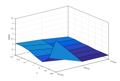
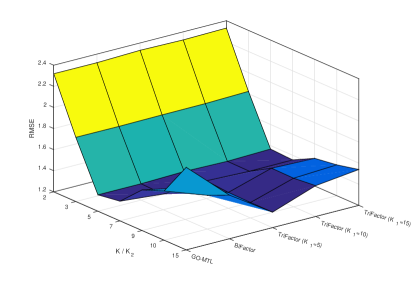
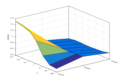
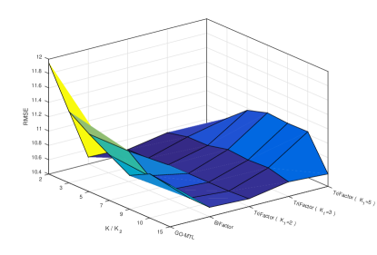
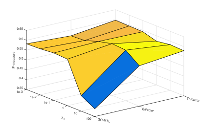
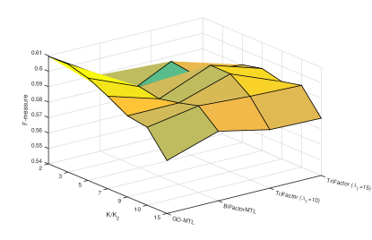
Figure 1: Top: Sensitivity analysis for the regularization parameter $\lambda_{2}$ when $\lambda_{1}=0.1$ and $K=2$ (left) and number of clusters $K_{1}$ and $K_{2}$ when $\lambda_{1}=0.1$ and $\lambda_{2}=0.1$ (right) calculated for syn5 dataset (RMSE). Middle: Sensitivity analysis for school dataset (RMSE). Bottom: Sensitivity analysis for sentiment detection (F-measure).

Additional Results

Tables 5 and 6 show the complete experimental results for sentiment analysis and transfer learning experiments.

List of one-vs-one classification tasks used in Table 6

(Task 1) comp.windows.x
vs comp.os.ms-windows.misc
(Task 2) soc.religion.christian
vs rec.sport.hockey
(Task 3) misc.forsale
vs talk.politics.guns
(Task 4)sci.med
vs rec.autos
(Task 5) comp.sys.mac.hardware
vs talk.politics.misc
(Task 6) sci.space
vs alt.atheism
(Task 7) comp.graphics
vs comp.sys.ibm.pc.hardware
(Task 8) talk.politics.mideast
vs sci.electronics
(Task 9) rec.motorcycles
vs talk.religion.misc
(Task 10) rec.sport.baseball
vs sci.crypt

Table 5: Performance results (F-measure) for various experiments on sentiment detection. The table reports the mean and standard errors over $5$ random runs.

Data	i@	ii@	iii@	iv@	v@	vi@	vii@
Tasks	14	28	56	84	42	86	126
Thresholds (Splits)	1 (1)	2 (2)	2 (4)	2 (6)	3 (3)	3 (6)	3 (9)
Train Size	240	120	60	40	80	40	26
STL	0.749 (0.003)	0.429 (0.002)	0.432 (0.001)	0.429 (0.002)	0.400 (0.002)	0.399 (0.003)	0.397 (0.001)
ITL	0.713 (0.002)	0.433 (0.001)	0.440 (0.002)	0.431 (0.001)	0.499 (0.001)	0.486 (0.002)	0.479 (0.001)
SHAMO	0.721 (0.005)	0.423 (0.002)	0.437 (0.006)	0.429 (0.002)	0.498 (0.006)	0.460 (0.002)	0.496 (0.013)
CMTL	0.713 (0.002)	0.557 (0.016)	0.436 (0.007)	0.429 (0.004)	0.508 (0.002)	0.486 (0.002)	0.476 (0.002)
MTFL	0.711 (0.002)	0.482 (0.004)	0.473 (0.002)	0.432 (0.007)	0.522 (0.002)	0.487 (0.003)	0.481 (0.002)
GO-MTL	0.638 (0.006)	0.582 (0.012)	0.526 (0.013)	0.516 (0.007)	0.587 (0.004)	0.540 (0.005)	0.539 (0.008)
BiFactorMTL	0.722 (0.006)	0.611 (0.018)	0.561 (0.013)	0.598 (0.002)	0.643 (0.013)	0.578 (0.020)	0.574 (0.052)
TriFactorMTL	0.733 (0.006)	0.627 (0.008)	0.588 (0.006)	0.603 (0.012)	0.655 (0.013)	0.606 (0.020)	0.632 (0.029)

Table 6: Performance results (F-measure) on 20Newsgroups dataset. The table reports the mean and standard errors over $5$ random runs. The best model and the statistically competitive models (by paired t-test with $\alpha=0.05$) are shown in boldface.

Models	Task 1	Task 2	Task 3	Task 4	Task 5	Task 6	Task 7	Task 8	Task 9	Task 10
GO-MTL	0.42 (0.09)	0.57 (0.06)	0.42 (0.04)	0.47 (0.06)	0.40 (0.03)	0.37 (0.02)	0.35 (0.02)	0.70 (0.01)	0.38 (0.00)	0.42 (0.05)
BiFactorMTL	0.42 (0.09)	0.60 (0.05)	0.41 (0.04)	0.49 (0.03)	0.36 (0.01)	0.42 (0.02)	0.37 (0.02)	0.64 (0.02)	0.38 (0.00)	0.46 (0.04)
TriFactorMTL	0.49 (0.03)	0.63 (0.02)	0.54 (0.02)	0.54 (0.02)	0.51 (0.02)	0.67 (0.01)	0.47 (0.02)	0.66 (0.01)	0.59 (0.03)	0.62 (0.01)

References

- Amit et al. (2007) Amit, Yonatan, Fink, Michael, Srebro, Nathan, and Ullman, Shimon. Uncovering shared structures in multiclass classification. In Proceedings of the 24th international conference on Machine learning, pp. 17–24. ACM, 2007.
- Argyriou et al. (2008) Argyriou, Andreas, Evgeniou, Theodoros, and Pontil, Massimiliano. Convex multi-task feature learning. Machine Learning, 73(3):243–272, 2008.
- Barzilai & Crammer (2015) Barzilai, Aviad and Crammer, Koby. Convex multi-task learning by clustering. In Proceedings of the 18th International Conference on Artificial Intelligence and Statistics (AISTATS-15), 2015.
- Crammer & Mansour (2012) Crammer, Koby and Mansour, Yishay. Learning multiple tasks using shared hypotheses. In Advances in Neural Information Processing Systems, pp. 1475–1483, 2012.
- Ding & He (2004) Ding, Chris and He, Xiaofeng. K-means clustering via principal component analysis. In Proceedings of the twenty-first international conference on Machine learning, pp. 29. ACM, 2004.
- Ding et al. (2006) Ding, Chris, Li, Tao, Peng, Wei, and Park, Haesun. Orthogonal nonnegative matrix t-factorizations for clustering. In Proceedings of the 12th ACM SIGKDD international conference on Knowledge discovery and data mining, pp. 126–135. ACM, 2006.
- Dinuzzo et al. (2011) Dinuzzo, Francesco, Ong, Cheng S, Pillonetto, Gianluigi, and Gehler, Peter V. Learning output kernels with block coordinate descent. In Proceedings of the 28th International Conference on Machine Learning (ICML-11), pp. 49–56, 2011.
- Gu & Zhou (2009) Gu, Quanquan and Zhou, Jie. Co-clustering on manifolds. In Proceedings of the 15th ACM SIGKDD international conference on Knowledge discovery and data mining, pp. 359–368. ACM, 2009.
- Jalali et al. (2010) Jalali, Ali, Sanghavi, Sujay, Ruan, Chao, and Ravikumar, Pradeep K. A dirty model for multi-task learning. In Advances in Neural Information Processing Systems, pp. 964–972, 2010.
- Kumar & Daume (2012) Kumar, Abhishek and Daume, Hal. Learning task grouping and overlap in multi-task learning. In Proceedings of the 29th International Conference on Machine Learning (ICML-12), pp. 1383–1390, 2012.
- Li & Ding (2006) Li, Tao and Ding, Chris. The relationships among various nonnegative matrix factorization methods for clustering. In Data Mining, 2006. ICDM’06. Sixth International Conference on, pp. 362–371. IEEE, 2006.
- Liu et al. (2009) Liu, Jun, Ji, Shuiwang, and Ye, Jieping. Multi-task feature learning via efficient l 2, 1-norm minimization. In Proceedings of the twenty-fifth conference on uncertainty in artificial intelligence, pp. 339–348. AUAI Press, 2009.
- Maurer et al. (2013) Maurer, Andreas, Pontil, Massimiliano, and Romera-Paredes, Bernardino. Sparse coding for multitask and transfer learning. In ICML (2), pp. 343–351, 2013.
- Raina et al. (2006) Raina, Rajat, Ng, Andrew Y, and Koller, Daphne. Constructing informative priors using transfer learning. In Proceedings of the 23rd International Conference on Machine Learning, pp. 713–720. ACM, 2006.
- Rothman et al. (2010) Rothman, Adam J, Levina, Elizaveta, and Zhu, Ji. Sparse multivariate regression with covariance estimation. Journal of Computational and Graphical Statistics, 19(4):947–962, 2010.
- Sindhwani et al. (2009) Sindhwani, Vikas, Hu, Jianying, and Mojsilovic, Aleksandra. Regularized co-clustering with dual supervision. In Advances in Neural Information Processing Systems, pp. 1505–1512, 2009.
- Sindhwani et al. (2013) Sindhwani, Vikas, Minh, Ha Quang, and Lozano, Aurélie C. Scalable matrix-valued kernel learning for high-dimensional nonlinear multivariate regression and granger causality. In Proceedings of the Twenty-Ninth Conference on Uncertainty in Artificial Intelligence, pp. 586–595. AUAI Press, 2013.
- Swirszcz & Lozano (2012) Swirszcz, Grzegorz and Lozano, Aurelie C. Multi-level lasso for sparse multi-task regression. In Proceedings of the 29th International Conference on Machine Learning (ICML-12), pp. 361–368, 2012.
- Wang et al. (2011) Wang, Hua, Nie, Feiping, Huang, Heng, and Makedon, Fillia. Fast nonnegative matrix tri-factorization for large-scale data co-clustering. In Proceedings of the 22nd International Joint Conference on Artificial Intelligence, pp. 1553, 2011.
- Weinberger et al. (2009) Weinberger, Kilian, Dasgupta, Anirban, Langford, John, Smola, Alex, and Attenberg, Josh. Feature hashing for large scale multitask learning. In Proceedings of the 26th Annual International Conference on Machine Learning, pp. 1113–1120. ACM, 2009.
- Xu et al. (2015) Xu, Linli, Huang, Aiqing, Chen, Jianhui, and Chen, Enhong. Exploiting task-feature co-clusters in multi-task learning. In Proceedings of the Twenty-Ninth AAAI Conference on Artificial Intelligence, pp. 1931–1937. AAAI Press, 2015.
- Xue et al. (2007) Xue, Ya, Liao, Xuejun, Carin, Lawrence, and Krishnapuram, Balaji. Multi-task learning for classification with dirichlet process priors. The Journal of Machine Learning Research, 8:35–63, 2007.
- Zhang et al. (2005) Zhang, Jian, Ghahramani, Zoubin, and Yang, Yiming. Learning multiple related tasks using latent independent component analysis. In Advances in neural information processing systems, pp. 1585–1592, 2005.
- Zhang & Schneider (2010) Zhang, Yi and Schneider, Jeff G. Learning multiple tasks with a sparse matrix-normal penalty. In Advances in Neural Information Processing Systems, pp. 2550–2558, 2010.
- Zhang & Yeung (2014) Zhang, Yu and Yeung, Dit-Yan. A regularization approach to learning task relationships in multitask learning. ACM Transactions on Knowledge Discovery from Data (TKDD), 8(3):12, 2014.
- Zhong & Kwok (2012) Zhong, Wenliang and Kwok, James T. Convex multitask learning with flexible task clusters. In Proceedings of the 29th International Conference on Machine Learning (ICML-12), pp. 49–56, 2012.