Cosmological Perturbations in the 5D Holographic Big Bang Model

Abstract

The 5D Holographic Big Bang is a novel model for the emergence of the early universe out of a 5D collapsing star (an apparent white hole), in the context of Dvali-Gabadadze-Porrati (DGP) cosmology. The model does not have a big bang singularity, and yet can address cosmological puzzles that are traditionally solved within inflationary cosmology. In this paper, we compute the exact power spectrum of cosmological curvature perturbations due to the effect of a thin atmosphere accreting into our 3-brane. The spectrum is scale-invariant on small scales and red on intermediate scales, but becomes blue on scales larger than the height of the atmosphere. While this behaviour is broadly consistent with the non-parametric measurements of the primordial scalar power spectrum, it is marginally disfavoured relative to a simple power law (at 2.7$\sigma$ level). Furthermore, we find that the best fit nucleation temperature of our 3-brane is at least 3 orders of magnitude larger than the 5D Planck mass, suggesting an origin in a 5D quantum gravity phase.

1 Introduction

Modern cosmology continues to experience an astonishing degree of empirical success [1]. The agreement with the phenomenological six-parameter $\Lambda$CDM paradigm is remarkable, all the more so as the number of cosmological observations continue to increase at an accelerated rate.

Despite this success, there are still intriguing puzzles left unresolved: the big bang singularity, the horizon and flatness problems (traditionally addressed within the inflationary paradigm), as well as the nature of dark matter and dark energy. Recently [2], a novel cosmological model was proposed in which our universe is a 3-brane emergent from the collapse of a 5-dimensional star. Motivated by the desire to see if a more satisfactory (or natural) understanding of these puzzles can emerge from an alternative description of the geometry, this model explains the evolution of our early universe whilst avoiding a big bang singularity. Furthermore, the model was shown to have a mechanism via which a homogeneous atmosphere outside the black hole generates a scale invariant power spectrum for primordial curvature perturbations, (nearly) consistent with current cosmological observations [1].

Our 5D holographic origin for the big bang is based on a braneworld theory that includes both 4 dimensional induced gravity and 5D bulk gravity: the Dvali-Gabadadze-Porrati (DGP) model [3], with action

$$S_{DGP}=\frac{1}{16\pi G_{5}}\int_{\text{bulk}}\!\!\!d^{5}x\sqrt{-g}R_{5}+\frac{1}{8\pi G_{5}}\int_{\text{brane}}\!\!\!d^{4}x\sqrt{-\gamma}K+\int_{\text{brane}}\!\!\!\sqrt{-\gamma}\bigg{(}\frac{R_{4}}{16\pi G_{4}}+{\cal{L}}_{\text{matter}}\bigg{)}\,,$$ (1.1)

where $g$ and $\gamma$, $G_{5}$ and $G_{4}$, $R_{5}$ and $R_{4}$ are the metrics, gravitational constants and Ricci scalars of the bulk and brane respectively, while $K$ is the mean extrinsic curvature of the brane. Our universe, described by the metric

$$ds^{2}_{4}=-d\tau^{2}+\frac{a^{2}(\tau)}{{\cal{K}}}[d\psi^{2}+\sin^{2}(\psi)(d\theta^{2}+\sin^{2}(\theta)d\phi^{2})]\,,$$ (1.2)

is represented by a hypersurface in a 5 dimensional Schwarzschild black hole spacetime

$$ds^{2}_{5}=-\left(1-\frac{\mu}{r^{2}}\right)dt^{2}+\left(1-\frac{\mu}{r^{2}}\right)^{-1}dr^{2}+r^{2}d\Omega_{3}^{2}~{},$$ (1.3)

located at $r=\frac{a(\tau)}{\sqrt{{\cal{K}}}}$. In this context, a pressure singularity is generically found when the energy density of the holographic fluid $\tilde{\rho}$ satisfies $\tilde{\rho}=\tilde{\rho}_{s}=\frac{3G_{4}}{16\pi G_{5}^{2}}$ [4]. The authors in [2] showed that the singularity happens at early times in the cosmic history as matter decays more slowly than $a^{-4}$. However, under the evolution from smooth initial conditions, the pressure singularity can occur before Big Bang Nucleosynthesis (BBN), and is generically inside a white hole horizon. Alternatively, the universe could have emerged from the collapse of a 5D star into a black hole, just before BBN, removing both pressure and big bang/white hole singularities. As advocated in the fuzzball program [5], the rate of this tunnelling is enhanced due to the large entropy of black hole microstates, which we speculate could match those of an expanding 3-brane thermal state. Our universe is represented by the boundary of a 5D spherically symmetric spacetieme with metric (1.3), in which we impose ${\mathbb{Z}}_{2}$ boundary conditions. This picture will be described in more detail in Section 2.

Interestingly, this model not only circumvents the singularity at the origin of time, but can also address other problems of cosmology that are typically solved by inflation. Because the collapsing star could have existed long before its demise, it had enough time to attain uniform temperature, thereby addressing the Horizon Problem. Furthermore, if we assume that the initial Hubble constant was of order of the 5D Planck mass, then the curvature density $-\Omega_{k}\sim(M_{5}r_{h})^{-2}$, where $r_{h}$ is the radius of the black hole. Consequently $-\Omega_{k}\sim M_{5}/M_{*}$ could become very small for massive stars, thus solving the Flatness Problem. More generically, the no hair theorem ensures that a 3-brane nucleated just outside the event horizon of a massive black hole has a smooth geometry.

Yet another feature of the model is that a thermal atmosphere around the brane, composed of a gas of massless particles produces scale invariant curvature perturbations. In this work, we shall revisit this result, focusing our attention on the mechanism responsible for deviations from scale-invariance in the primordial curvature power spectrum in the context of the 5D Holographic origin of the Big Bang. To this end, we consider a thin atmosphere that can be regarded as infalling matter, or the outer envelope of the collapsing 5D star, which resides in the 5D bulk and thus contributes to its energy momentum tensor. In this context, the DGP action Eq. (1.1) is modified to

$$S=S_{DGP}+\int_{\text{bulk}}d^{5}x\sqrt{-g}{\cal{L}}_{\text{5,atmosphere}}$$ (1.4)

where ${\cal{L}}_{\text{5,atmosphere}}$ accounts for the matter Lagrangian in the bulk. Consistency between cosmological phenomenology and the DGP model implies that the brane is expanding outwards, and thus eventually encounters this atmosphere. We then compute the resulting power spectrum of scalar curvature perturbations and the change of the Hubble parameter due to this encounter. We find that the best fit nucleation temperature of the 3-brane is considerably larger than the 5D Planck mass, perhaps indicating an origin in a 5D quantum gravity phase.

In Section 2, we discuss a possible mechanism for brane nucleation and the different scales involved in our problem, giving a qualitative description of the different physics processes. In Section 3, we solve Einstein equations with matter in the bulk, and the consequences that it has on the brane. In particular, we solve for the density profile of a 5D spherically collapsing atmosphere and compute the change on the Hubble parameter as it falls into our 3-brane. In Section 4, we study cosmological perturbations in the bulk and their projection onto the brane, making special emphasis on the curvature perturbation and its power spectrum. Section 5 compares our predictions against Planck data and contrasts it with the power-law power spectrum assumed in the $\Lambda$CDM model. We conclude our work with discussion of the limitations and prospects of our model in Section 6.

2 A 5D Holographic Big Bang

2.1 Brane Nucleation

As described in the introduction, we are working in the context of the 5D Holographic Big Bang model [2] where our universe is modelled as a hypersurface (the brane) in a 5-dimensional Schwarzschild space time according to the embedding $r=\frac{a(\tau)}{\sqrt{{\cal{K}}}}$. This construction is a solution of the DGP action (1.1) once we impose a $\mathbb{Z}_{2}$ boundary condition on the brane. As a consequence, via the embedding constraint the brane becomes an outward travelling boundary of the higher dimensional spacetime, an assumption that is necessary if we want our universe (represented by the brane) to be expanding.

From the perspective of an observer in the bulk, this setup is reminiscent of a construction proposed by Witten called the ‘bubble of nothing’ [6], in which an interior region of space is missing, with space ending smoothly at the surface of this bubble (the brane). One possible scenario in the 5D Holographic Big Bang model is that the brane was formed by the quantum tunnelling of a collapsing star in 5 dimensions, with all of the degrees of freedom of the inner part of the collapsing matter becoming degrees of freedom of the brane. This is analogous to the fuzzball paradigm, a model proposed to solve the information-loss paradox [7], which consists of the explicit construction of black hole microstates with no “dataless horizon region”. The infalling matter can tunnel to a fuzzball state with amplitude [5]

$${\cal{A}}\sim e^{-\frac{1}{G_{5}}\int R}\sim e^{-\alpha G_{5}M^{3}}\,,$$ (2.1)

where $\alpha={\cal{O}}(1)$ and we have used the length scale $r\sim G_{5}M^{2}$ to estimate the Euclidean Einstein action for tunneling between two configurations that have the length and mass scales set to those of the black hole. Although this amplitude is very small, the number of fuzzball configurations that a black hole can tunnel to depends on the Bekenstein-Hawking entropy as

$${\cal{N}}\sim e^{S_{BH}}\sim e^{G_{5}M^{3}}$$ (2.2)

yielding a significant probability to form a fuzzball. In fact, the two exponentials exactly cancel each other [5]. We anticipate a similar principle operating here, in which collapsing matter at sufficiently high density – just prior to formation of a black hole horiozn– necessarily tunnels to a brane so as to avoid the ensuing quantum paradoxes that follow upon introducing an event horizon.

Since it is well established that BBN happened in the formation of our universe, and that in the 5D Holographic Big Bang (HBB) model [2] the pressure singularity generically forms before BBN, we consider a brane that must form before this. This means that the temperature of nucleation must be at most the temperature of BBN – $T_{\rm BBN}\sim 0.4\,\text{MeV}$ [8]:

$$T_{\rm nuc}\geq T_{\rm BBN}\sim 0.4~{}{\rm MeV}.$$ (2.3)

Finally, let us mention that the DGP model possesses a scale $r_{c}=\frac{G_{5}}{G_{4}}$, above which 5-dimensional gravity dominates over 4-dimensional gravity. Constraints on the normal branch of the DGP model [9] give

$$r_{c}\gtrsim 3H_{0}^{-1}\,\,\,\,\,\,\,\,\,\to\,\,\,\,\,\,\,\,M_{5}<(H_{0}M_{4}^{2}/12)^{1/3}\,\,\,\,\,\,\,\,\to\,\,\,\,\,\,\,\,M_{5}<9\,\text{MeV}\,.$$ (2.4)

where $M_{4}=\frac{1}{(8\pi G_{4})^{1\!/2}}$ is the reduced 4D Planck mass.

2.2 The Atmosphere: Setup and Scales

Figure 1: Cartoon of the different scales treated in this problem, in the black hole rest frame. The inner black circular arc represents the brane with radius $R$ and the outer black circular arc represents the brane with radius $2R$. $H^{-1}$ is estimated by tracing light rays on the brane after it has doubled it size; it is small if the brane is traveling near the speed of light. The atmosphere is shown in yellow sitting in between the two red arcs with length $\Delta L$.

In this scenario, we are interested in the effects of a thin atmosphere located just outside the brane. Although the brane forms a $\mathbb{Z}_{2}$ boundary, excluding the event horizon in Eq. (1.3), we shall refer to the metric in Eq. (1.3) as the black hole metric.

In order to organize the different assumptions, we will review the implied hierarchy of the scales present in this problem. If we assume that the Hubble patch of our universe, at/near brane nucleation, is small enough to be insensitive to the curvature of the black hole spacetime, we can assume that the atmosphere is just a perturbation around a Minkowski background. This limit implies $H^{-1}\ll R$ where R is the radius of the black hole, or brane upon nucleation. This assumption is also observationally motivated, since today we measure $(HR)^{-2}\ll|\Omega_{k}|\ll 1$ and thus our observable Hubble patch is approximately flat. In our model, if the brane is moving very close to the speed of light, $H^{-1}\ll R$. This will allow us to define metric perturbations in Section 4. We will then be interested in finding the behaviour of the power spectrum of curvature perturbations for modes of wavelength $\lambda$, that are of super-horizon size before BBN, but are now observable in the CMB sky. This restricts $R\gg\lambda\gg H^{-1}$.

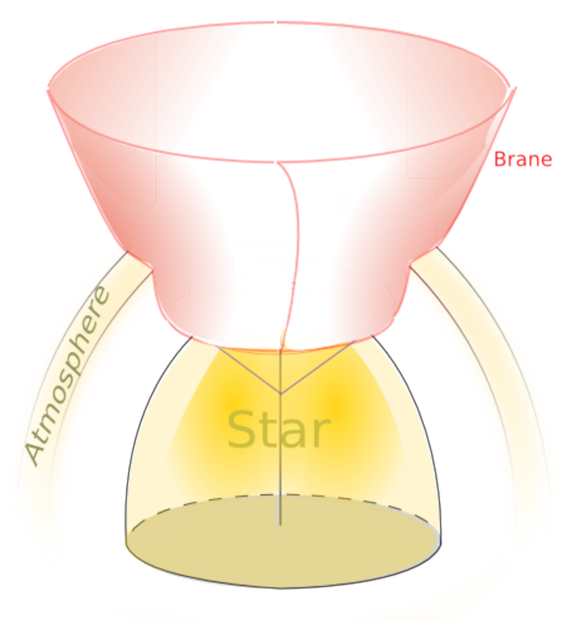
Finally, we would like to understand the behaviour of different physical quantities of the brane, such as the behaviour of the Hubble parameter before and after the encounter with the atmosphere. Assuming it can be considered to be a thin atmosphere in the 5 dimensional space time, the width $\Delta L$ of the atmosphere needs to be smaller than $R$ for the brane to cross the atmosphere completely in less than a Hubble time. We then get the following hierarchy of different scales

$$H^{-1}\ll\lambda\ll R,~{}{\rm and}~{}\Delta L\ll R{\rm~{}(black~{}hole~{}frame)},$$ (2.5)

$$\lambda\lesssim\Delta L{\rm~{}(atmosphere~{}frame)}.$$ (2.6)

As we shall in Section 4, the latter inequality is the key ingredient that leads to a near scale-invariant spectrum of primordial curvature perturbations for large scales. This hierarchy of scales is illustrated in Fig. 1.

3 Homogeneous brane meets thin atmosphere

3.1 Einstein Equations

We want to study the influence of an atmosphere that is falling into the black hole as shown in in Fig. 2. For this, we assume that the brane is moving supersonically (in fact, almost with the speed of light) into the atmosphere, and thus bulk metric perturbations do not react to the brane’s presence until it runs into them.

Figure 2: Penrose diagram (left), and cartoon of the 5D star collapse (right), followed by the nucleation of a 3-brane (our universe). The star (in yellow) that is collapsing (nearly) forms a black hole, but the 3-brane (red) will nucleate just prior to the formation of the event horizon, and traverses a thin atmosphere of infalling matter or atmosphere (cross-section shown in the cartoon at right).

The Einstein equations on the brane that follow from the action (1.4) are:

$$G_{\mu\nu}=8\pi G_{4}\left(T_{\mu\nu}+\tilde{T}_{\mu\nu}\right)$$ (3.1)

where the two different components of the energy-momentum tensor are $T_{\mu\nu}$, the matter living on the brane, and $\tilde{T}_{\mu\nu}$ the holographic fluid that is induced on the brane via the junction conditions described below. Due to the symmetry of the (unperturbed) FRW spacetime, $T_{\mu\nu}$ has the form of a perfect fluid

$$T_{\mu\nu}=\left(P+\rho\right)u_{\mu}u_{\nu}+P\gamma_{\mu\nu}\,,$$ (3.2)

where $u^{\mu}$ is the 4-velocity of the fluid normalized such that $u^{\mu}u_{\mu}=-1$.

The holographic fluid is the Brown-York stress tensor induced on the brane once Einstein equations are imposed on the bulk

$$\tilde{T}_{\mu\nu}=\frac{1}{8\pi G_{5}}\left(K\gamma_{\mu\nu}-K_{\mu\nu}\right),$$ (3.3)

where $K_{\mu\nu}\equiv\nabla_{\alpha}n_{\beta}e^{\alpha}_{\mu}e^{\beta}_{\nu}$ is the extrinsic curvature of the brane whose unit normal is $n^{\alpha}$. Here $e^{\alpha}_{\nu}\equiv\frac{\partial\hat{x}^{\alpha}}{\partial x^{\nu}}$, where we have associated the set of coordinates $\{\hat{x}^{\alpha}\}$ and $\{x^{\nu}\}$ with the bulk and the brane respectively. In addition to the Einstein equations (3.1), the continuity equations for the total matter living on the brane arising from the Bianchi identities are:

$$\nabla^{\mu}\left(T_{\mu\nu}+\tilde{T}_{\mu\nu}\right)=0\,.$$ (3.4)

The Gauss-Codazzi equations constrain the geometric quantities of the brane with the matter present in the bulk

$$\nabla^{\mu}\left(Kg_{\mu\nu}-K_{\mu\nu}\right) = 8\pi G_{5}T^{5}_{\alpha\beta}e^{\alpha}_{\nu}n^{\beta}\,,$$ (3.5)

$$R^{4}+K^{\mu\nu}K_{\mu\nu}-K^{2} = -16\pi G_{5}T^{5}_{\alpha\beta}n^{\alpha}n^{\beta}\,,$$ (3.6)

where $R^{4}=-8\pi G_{4}\left(T+\tilde{T}\right)$ is the Ricci scalar of the brane. $T^{5}_{\alpha\beta}$ is the energy momentum tensor of the bulk which satisfies the Einstein’s equations on the bulk $G_{\alpha\beta}=8\pi G_{5}T^{5}_{\alpha\beta}$. Note that the first of the Gauss-Codazzi equations (3.5) reduces to the conservation of the holographic fluid $\tilde{T}_{\mu\nu}$ in the case that $T^{5}_{\alpha\beta}=0$. If the bulk matter flows into the brane, the holographic fluid is not conserved and the effect of the continuity equation (3.4) is to change the matter on the brane through the holographic fluid in order for the sum of both to be conserved.

In the same way, as a result of the symmetries of FRW spacetime, the holographic fluid must have the form of a perfect fluid. Moreover, the 4-velocity of this fluid must coincide with the 4-velocity of the normal matter on the brane:

$$\tilde{T}_{\mu\nu}=\left(\tilde{P}+\tilde{\rho}\right)u_{\mu}u_{\nu}+\tilde{P}\gamma_{\mu\nu}\,.$$ (3.7)

Combining Eqs. (3.3) and (3.7) we get:

$$K_{\mu\nu}=-8\pi G_{5}\bigg{[}\left(\tilde{P}+\tilde{\rho}\right)u_{\mu}u_{\nu}+\frac{1}{3}\tilde{\rho}_{\mu\nu}\bigg{]}\,.$$ (3.8)

3.2 Shift in the Hubble

The rate of expansion described by the Hubble parameter will change as the brane goes through the atmosphere and we can find a general expression for $H$ by studying the Einstein equations and junction conditions for the DGP brane in the general case. This general case treats the bulk as a 5-dimensional Schwarzschild black hole (1.3) and the brane as a hypersurface parametrized by $r=\frac{a(\tau)}{\sqrt{{\cal{K}}}}$, as detailed in the Introduction.

From Equations (3.1) and (3.4-3.6) we obtain

$$H^{2}+\frac{\cal{K}}{a^{2}}=\frac{8\pi G_{4}}{3}\left(\tilde{\rho}+\rho\right)$$ (3.9)

$$\dot{\rho}+\dot{\tilde{\rho}}+3H\left(\rho+\tilde{\rho}+P+\tilde{P}\right)=0$$ (3.10)

$$\dot{\tilde{\rho}}+3H\left(\tilde{\rho}+\tilde{P}\right)=T^{5}_{\alpha\beta}e^{\alpha}_{\tau}n^{\beta}$$ (3.11)

$$0=T^{5}_{\alpha\beta}e^{\alpha}_{i}n^{\beta}$$ (3.12)

$$\left(\rho+\tilde{\rho}\right)-3\left(P+\tilde{P}\right)+\frac{8\pi G_{5}^{2}}{G_{4}}\left(\frac{2}{3}\tilde{\rho}^{\,2}+2\tilde{P}\tilde{\rho}\right)=-2\frac{G_{5}}{G_{4}}T^{5}_{\alpha\beta}n^{\alpha}n^{\beta}$$ (3.13)

The quantity $T^{5}_{\alpha\beta}$ is the stress-energy of the atmosphere outside the black hole. This atmosphere will have two effects on the brane. It will induce metric and matter perturbations in our universe, which we shall use to compute the curvature perturbation in Sec. 4 below. However it will also make the Hubble parameter change its value as the brane crosses the atmosphere: the brane will expand more slowly due to an extra source of infalling matter. Combining Eqs. (3.9) and (3.10) and ignoring the curvature term we get

$$\Delta H=-4\pi G_{4}\int(P_{T}+\rho_{T})\,d\tau,\,$$ (3.14)

where the integral is performed in the proper time of the brane and $P_{T}=P+\tilde{P}$, $\rho_{T}=\rho+\tilde{\rho}$.

Let’s first look at the behavior of the holographic fluid $\tilde{P}$ and $\tilde{\rho}$. From Equation (3.13) we have

$$\tilde{P}+\tilde{\rho}=\frac{1}{3\big{(}\frac{\tilde{\rho}}{\tilde{\rho}_{s}}-1\big{)}}\bigg{[}-2\frac{G_{5}}{G_{4}}T^{5}_{nn}-4\tilde{\rho}+2\frac{\tilde{\rho}^{2}}{\tilde{\rho}_{s}}+T\bigg{]}\,,$$ (3.15)

where $T=3P-\rho$, $T^{5}_{nn}=T^{5}_{\alpha\beta}n^{\alpha}n^{\beta}$ and $\tilde{\rho}_{s}=\frac{3G_{4}}{16\pi G_{5}^{2}}$. In order to avoid the pressure singularity we require $\tilde{\rho}\gg\tilde{\rho}_{s}$ and in this limit the last equation becomes

$$\tilde{P}+\tilde{\rho}=\frac{1}{3}\bigg{[}-2\frac{G_{5}}{G_{4}}T^{5}_{nn}\frac{\tilde{\rho}_{s}}{\tilde{\rho}}+2\tilde{\rho}+T\frac{\tilde{\rho}_{s}}{\tilde{\rho}}\bigg{]}\,.$$ (3.16)

Now let’s analyze the behavior for the the matter on the brane $P$ and $\rho$. Combining Eqs. (3.10) and (3.11) and assuming an equation of state $P=w\rho$ the fluid on the brane satisfies

$$\dot{{\rho}}+3H\left({\rho}+{P}\right)=-T^{5}_{\alpha\beta}e^{\alpha}_{\tau}n^{\beta}\Rightarrow\frac{d}{d\tau}(\rho a^{3(w+1)})=-T^{5}_{\alpha\beta}e^{\alpha}_{\tau}n^{\beta}a^{3(w+1)}\,.$$ (3.17)

If we now assume that the atmosphere is thin enough so that we can approximate the matter distribution as a delta function (i.e. $H\Delta\tau\ll 1$, during the impact time $\Delta\tau$), we see that the last equation will give a jump in the density (and hence in the pressure) proportional to a step function. In fact, if we consider the system of equations (3.9-3.13), with $P=w\rho$, and a delta function $T^{5}_{\alpha\beta}$, the only consistent solution would have a delta function in $\tilde{P}$, with step function jumps in other variables. As such, the biggest contribution in Eq. (3.14) is given by the first term on the right hand side of Eq. (3.16):

$$\Delta H=\frac{G_{4}}{2G_{5}}\int\frac{T^{5}_{\alpha\beta}n^{\alpha}n^{\beta}}{\tilde{\rho}}d\tau\left[1+{\cal O}(H\Delta\tau)\right]\,.$$ (3.18)

We shall see in Sec. 4 below that the amplitude of curvature perturbations depends on $\Delta\ln H=\frac{\Delta H}{H}$. To compute this, we note that from Eq. (3.9) we can write $H^{2}\approx\frac{8\pi G_{4}}{3}(\tilde{\rho}+\rho)\approx\frac{8\pi G_{4}}{3}\rho$ in the regime where $\rho\gg\tilde{\rho}$. Then

$$\Delta\,\text{ln}H\approx\frac{G_{4}}{2G_{5}}\sqrt{\frac{3}{8\pi G_{4}}}\frac{1}{\sqrt{\rho}\tilde{\rho}}\int T^{5}_{\alpha\beta}n^{\alpha}n^{\beta}\,d\tau\,,$$ (3.19)

We can now use the solution in vacuum for $\tilde{\rho}$ found in [2]

$$\tilde{\rho}=\tilde{\rho}_{s}\bigg{(}1+\sqrt{1-\frac{2(\rho_{BH}-\rho)}{\tilde{\rho}_{s}}}\bigg{)}\,,$$ (3.20)

where $\rho_{BH}=\frac{3\Omega_{k}^{2}H_{0}^{4}r_{h}^{2}}{8\pi G_{4}a^{4}}$. In the approximation where $\rho\gg\rho_{BH}$ and $\rho\gg\tilde{\rho}_{s}$ we find

$$\tilde{\rho}\approx\rho\sqrt{\frac{2\tilde{\rho}_{s}}{\rho}}\,$$ (3.21)

and then Eq. (3.19) reads

$$\Delta\,\text{ln}H\approx\frac{1}{2\rho}\int T^{5}_{\alpha\beta}n^{\alpha}n^{\beta}d\tau\,,$$ (3.22)

implying that the relative jump in the Hubble parameter due to a thin atmosphere is the ratio of the work done by the pressure of the atmosphere to the energy of the brane.

3.3 Profile of the atmosphere

So far we have considered a general energy momentum tensor on the bulk responsible of dynamic features on the brane. Let’s now consider that the bulk is filled with a relativistic spherically symmetric, collapsing 5D radiation atmosphere ($P_{5}=\frac{1}{4}\rho_{5}$) that represents the atmosphere whose energy momentum tensor is

$$T_{\alpha\beta}^{5}(w)=\rho_{5}(w)\bigg{[}\bigg{(}1+\frac{1}{4}\bigg{)}\delta^{0}_{\alpha}\delta^{0}_{\beta}+\frac{1}{4}\eta_{\alpha\beta}\bigg{]}\,.$$ (3.23)

In order to study the effect of this atmosphere we need to introduce scalar homogeneous perturbations in the bulk. A generalization of 4D perturbation theory allows us to write the perturbed metric of the bulk in the Newtonian gauge in 5D as

$$ds^{2}_{\text{bulk}}=-[1+2\Phi_{5}(x^{\alpha})]dt^{2}+[1-2\Psi_{5}(x^{\alpha})][dx^{2}+dy^{2}+dz^{2}+dw^{2}]\,.$$ (3.24)

where $\Phi_{5}$ and $\Psi_{5}$ represent the scalar perturbations of the bulk and $x^{\alpha}$ are bulk coordinates. Our universe is represented as a hypersurface in the 5D bulk, whose trajectory is given by the constraint $w=f(x^{\mu})$. In this setup, the brane will inherit three bulk coordinates $\{t,x,y,z\}$ and will respond to perturbations that are just functions of the bulk time via the relation $w=f(x^{\mu})$. Consider that the metric perturbations and the brane position are homogeneous:

$$\Phi_{5}=\epsilon\Phi_{5}^{0}(w)\,,\quad\Psi_{5}=\epsilon\Psi_{5}^{0}(w)\,,\quad f=f_{0}(t)\,,$$ (3.25)

where $\epsilon\ll 1$ is a parameter that controls the homogeneous metric perturbations. Assuming hydrostatic equilibrium in the (infalling) rest frame of the atmosphere, the Einstein Equations in the bulk for the metric (3.24) leads to the relativistic Poisson and Euler equations:

$$\nabla^{2}\Phi_{5}^{0} = \frac{8\pi G_{5}}{3}\rho_{5}\,,$$ (3.26)

$$\nabla\Phi_{5}^{0} = -\frac{1}{4}\frac{\nabla\rho_{5}}{\rho_{5}}\,.$$ (3.27)

These equations can be solved exactly in Minkowski background:

$$\rho_{5}(w)=\bar{\rho}_{5}\bigg{\{}1-\tanh^{2}\bigg{[}\bar{\gamma}\bigg{(}\frac{w}{\bar{w}}-1\bigg{)}\bigg{]}\bigg{\}}\,,$$ (3.28)

where $\bar{\rho}_{5}\equiv\frac{3}{16\pi G_{5}}\frac{\bar{\gamma}^{2}}{\bar{w}^{2}}$, while $\bar{\gamma}$ and $\bar{w}$ are constants of integration.

The relationship between the energy density and the temperature of the atmosphere can be computed by integrating the Bose-Einstein distribution in 4+1 dimensions

$$\rho_{5}(w)=\int\frac{d^{4}k}{(2\pi)^{4}}\frac{\omega}{\exp\left[\omega/T_{5}(w)\right]-1}=\frac{3\zeta_{R}(5)}{\pi^{2}}T_{5}(w)^{5}\,,$$ (3.29)

where $\omega^{2}=k_{\alpha}k^{\alpha}$. The above expression allows us to write

$$T_{5}(w)=\bigg{(}\rho_{5}(w)\frac{\pi^{2}}{3\zeta_{R}(5)}\bigg{)}^{\frac{1}{5}}=1.26\,\rho_{5}(w)^{1/5}\,.$$ (3.30)

Note that the characteristic thickness of the atmosphere is given by

$$\Delta L=\frac{\bar{w}}{\sqrt{2}\bar{\gamma}}\,.$$ (3.31)

We are now in position to compute Eq. (3.22) and we will do so in the reference frame of the atmosphere. In this frame $\rho_{5}$ does not depend on time, but the normal to the brane $n^{\alpha}$ will depend on the relative velocity of the brane and the atmosphere. First consider the fluid velocity $u^{\alpha}=(1,{\bf{v}})/\sqrt{1-v^{2}}$, where v is the relative 3 velocity between the brane and the atmosphere. If we now require $n_{\alpha}n^{\alpha}=1$ and $n^{\alpha}u_{\alpha}=0$ we have $n^{\alpha}=(v,{\bf v}/v)/\sqrt{1-v^{2}}$. With this we can write $T^{5}_{\alpha\beta}n^{\alpha}n^{\beta}=\rho_{5}(w)(1+4v^{2})/4(1-v^{2})$ and the RHS of Eq. (3.22) reads

$$\Delta\,\text{ln}H=\frac{1}{2\rho}\int T^{5}_{\alpha\beta}n^{\alpha}n^{\beta}d\tau = \frac{1}{2\rho}\int_{0}^{\infty}T^{5}_{\alpha\beta}n^{\alpha}n^{\beta}\sqrt{1-v^{2}}dt\,,$$ (3.32)

$$= \frac{1}{2\rho}\int_{0}^{\infty}T^{5}_{\alpha\beta}n^{\alpha}n^{\beta}\sqrt{1-v^{2}}\frac{dw}{v}\,,$$

$$= \frac{(1+4v^{2})}{v\sqrt{1-v^{2}}}\frac{\bar{\rho}_{5}}{8\rho}\frac{\bar{w}}{\bar{\gamma}}\bigg{[}1+\tanh(\bar{\gamma})\bigg{]}\,.$$

4 Cosmological perturbations

As discussed in the last section, if the velocity of the brane is near the speed of light we can assume that the Hubble patch of the universe will be smaller than the curvature radius of the black hole spacetime. In this regime it is safe to approximate the bulk as Minkowski spacetime and analyze the perturbations around it. In the last section we have briefly introduced the homogeneous scalar perturbations and in Appendix A we present the anisotropic perturbations. The curvature perturbation can be written as function of the scalar gauge invariant quantities (A.8)

$$\zeta=\Psi_{4}-\frac{H}{\dot{H}}\bigg{(}H\Phi_{4}+\dot{\Psi}_{4}\bigg{)}\,.$$ (4.1)

Note that in our framework the Hubble constant is of first order in the perturbation (see Eq.(A.9)) as the brane crosses the atmosphere, and thus the term $H\Phi_{4}$ can be neglected. With this we have

$$\zeta\approx\Psi_{4}-\frac{\Delta\Psi_{4}}{\Delta\text{ ln}(H)}\,,$$ (4.2)

where $\Delta\Psi_{4}=\Psi_{4_{f}}-\Psi_{4_{i}}$. Here $\Psi_{4_{i(f)}}$ stands for the metric perturbation in 4D right before (after) the brane crossed the atmosphere, and we assume that $\zeta$ evolves continuously. We are interested in the value of the curvature perturbation after the brane has passed through the atmosphere where the metric perturbation $\Psi_{5_{f}}=0$, which makes $\Psi_{4_{f}}=0$. In this regime the curvature perturbation becomes

$$\zeta=\zeta_{f}\approx\frac{\Psi_{4i}}{\Delta\text{ ln}(H)}\,.$$ (4.3)

We are now ready to analyze the behaviour of the curvature perturbation power spectrum

$$P_{\zeta}(k)=\int d^{3}{\bf{x}}\,\,e^{i\bf{k\cdot x}}\langle\zeta(x)\zeta(0)\rangle\,.$$ (4.4)

If the atmosphere is not in thermal equilibrium, we can relate the 2-point correlation function of the thermal fluctuations in 5D energy density to the temperature profile of the atmosphere:

$$\langle\rho_{5}(y_{1})\rho_{5}(y_{2})\rangle=\alpha\,(T_{5}(y_{1}))^{6}\delta^{4}(y_{1}-y_{2})\,.$$ (4.5)

To proceed, we notice that in [2] it was found that the 5D energy density correlation function due to a thermal gas is

$$\left\langle\rho_{5}(y_{1})\rho_{5}(y_{2})\right\rangle\simeq\frac{5}{8}\bigg{[}\int\frac{d^{4}k}{(2\pi)^{4}}\bigg{[}\frac{1}{\text{exp}(\omega/T_{5})-1}+\frac{1}{2}\bigg{]}\,\omega\,\text{exp}[ik_{a}(y_{1}^{a}-y_{2}^{a})]\bigg{]}^{2}\,.$$ (4.6)

This expression can be approximated as a delta function $\left\langle\rho_{5}(y_{1})\rho_{5}(y_{2})\right\rangle\simeq\alpha(T_{5}(y_{1}))^{6}\delta^{4}(y_{1}-y_{2})$, where $\alpha=\frac{5}{8}\bigg{[}\frac{1}{\pi^{2}63}(945\zeta_{R}(5)-\pi^{6})\bigg{]}$, while we have dropped the power-law UV divergence and $\zeta_{R}$ is the Riemann zeta function. Note, that (4.6) can be approximated by a 4 dimensional delta function on length scales larger than the thermal wavelength $T^{-1}_{5}$.

With the use of the Poisson equation in 5D

$$\nabla^{2}\Psi_{5}(y)=\frac{8\pi G_{5}}{3}\rho_{5}(y)\,,$$ (4.7)

we can find the power spectrum for the curvature perturbation to be (see Appendix B for details)

$${\cal{P}}(k)=\frac{k^{3}}{2\pi^{2}}P_{\zeta}(k) = \beta\,k\int_{0}^{\infty}dw\,e^{-2|w|k}\,(T_{5}(w))^{6}$$ (4.8)

$$= \Delta_{0}^{2}\,k\int_{0}^{\infty}dw\,e^{-2|w|k}\,\left\{1-\tanh^{2}[\bar{\gamma}(w/\bar{w}-1)]\right\}^{6/5}$$ (4.9)

where $\Delta_{0}^{2}=\beta\,[\bar{T}_{5}]^{6}$, $\beta=\frac{\alpha}{2}\bigg{(}\!\frac{G_{5}}{6\Delta\text{ln}H\,\pi^{3}}\!\bigg{)}^{2}$ and we have used Eqs.(3.29) and (3.30) of Sec. 3.3 to write the temperature of the brane. The power spectrum predicted by our model is characterized by 3 free parameters ${\bar{\gamma},\bar{w},\Delta_{0}^{2}}$ which we are going to fit to Planck data in the next section.

5 Observational constraints on 5D holographic big bang

The standard model of cosmology, $\Lambda$CDM, is described by 6 parameters $(\Omega_{b}h^{2},\Omega_{c}h^{2},\theta,\tau,\Delta_{0}^{2},n_{s})$, the baryon density, dark matter density, angular size of the sound horizon at recombination, the optical depth to reionization, amplitude of the scalar power spectrum and its tilt respectively. This model characterizes early universe cosmology via the power spectrum of the curvature perturbations

$${\cal{P}}(k)=\Delta_{0}^{2}\bigg{(}\frac{k}{k_{*}}\bigg{)}^{n_{s}-1}\,,$$ (5.1)

where $k_{*}=0.05/\text{Mpc}$ is the comoving pivot scale. This form of the power spectrum, expected in slow-roll inflationary models, best fits the CMB data with parameter values [1]

$$\Delta_{0}^{2}=(2.196\pm 0.059)\times 10^{-9}\,\,\,\,\,\,\,\,\,\,\,n_{s}=0.9603\pm 0.0073\,.$$ (5.2)

We would like to compare this model with the HBB model (Eq. 4.9) that strictly is represented by the seven parameters $(\Omega_{b}h^{2},\Omega_{c}h^{2},\theta,\tau,\bar{\gamma},\bar{w},\Delta_{0}^{2})$. In order to compare models with the same number of parameters, will also include $\Lambda$CDM with running $\alpha_{s}=dn_{s}/d\,\text{ln}q$.

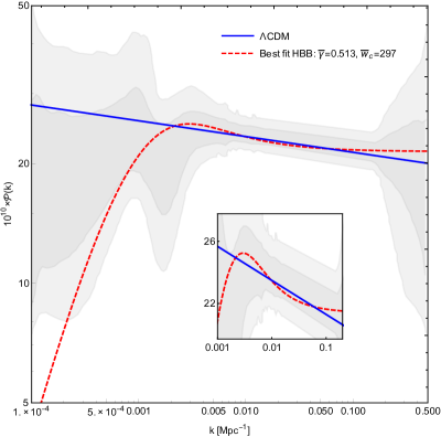
We have performed the comparison by running the CosmoMC code [11, 12, 13, 14, 15, 16, 17] with Planck 2015 data, Barionic Acoustic Oscillations (BAO) [18, 19, 20, 21, 22, 23, 24, 25] as well as lensing data [26, 27, 28, 29, 30]. Finally, to determine the best fit parameters and the likelihood, we run the minimizer expressing our results Table 1. Comparing best-fit $\chi^{2}$ of HBB and $\Lambda$CDM (with running), we see that HBB is disfavoured at roughly 2.7 2.8$\sigma$ (2.8$\sigma$). The Planck angular TT spectrum together with the best fit curves and residuals for HBB and $\Lambda$CDM are shown in Fig. 3. The best fit primordial scalar power spectrum in both models are also contrasted with a non-parametric reconstruction from Planck 2015 data [31]. We note that the difference between the two models (mostly) lies within the 68% region and the largest disagreement of the models is at low l’s or k’s.

Table 1: Planck 2015 and BAO best fit parameters and 68% ranges for HBB and $\Lambda$CDM models. The last row indicates the $\chi^{2}$ for each of the models. Note that $\bar{w}_{c}$ corresponds to the comoving value of the position of the centre of the atmosphere and its related to the physical $\bar{w}$ via $\bar{w}=\bar{w}_{c}\frac{2.3\times 10^{-10}\text{MeV}}{T_{\text{nuc}}}$.

	HBB		$\Lambda\text{CDM}$		$\Lambda\text{CDM}$ with running
	best fit	$68\%$ range	best fit	$68\%$ range	best fit	$68\%$ range
$\Omega_{b}h^{2}$	$0.02212$	$0.02210\pm 0.00023$	$0.02227$	$0.02225\pm 0.00020$	$0.02231$	$0.02229\pm 0.00022$
$\Omega_{c}h^{2}$	$0.1172$	$0.1169\pm 0.0012$	$0.1185$	$0.1186\pm 0.0012$	$0.1184$	$0.1186\pm 0.0012$
$100\theta$	$1.04113$	$1.04116\pm 0.00042$	$1.04103$	$1.04104\pm 0.00042$	$1.04108$	$1.04105\pm 0.00041$
$\tau$	$0.081$	$0.083\pm 0.014$	$0.067$	$0.067\pm 0.013$	$0.069$	$0.068\pm 0.013$
$10^{9}\Delta_{0}^{2}$	$5.79$	$0.793\pm 0.021$	$5.798$	$5.798\pm 0.019$	$5.82$	$5.82\pm 0.020$
$n_{s}$			$0.9682$	$0.9677\pm 0.0045$	$0.9682$	$0.9671\pm 0.0045$
$\alpha_{s}$					$-0.0027$	$-0.0030\pm 0.0074$
$\bar{\gamma}$	$0.513$	$0.525\pm 0.053$
$\bar{w}_{c}\,[\text{Mpc}]$	$275$	$297_{-77}^{+39}$
$\chi^{2}$	$11327.4$		$11319.9$		$11319.6$

Figure 3: Left-Top: angular power spectrum of CMB temperature anisotropies, comparing Planck 2015 data (black dots) with best HBB model (solid/red) for all l. Left-Inset: angular power spectrum of CMB temperature anisotropies, comparing Planck 2015 data with $\Lambda$CDM (dotted/blue) and HBB (solid/red) for $l<40$. Left-Bottom: relative residuals and difference between $\Lambda$CDM and HBB (black solid) where the green shaded region indicates the 68% region of Planck 2015 data. Right: Best fit of the primordial power spectrum as predicted by HBB (dashed-red) in comparison with the best fit of $\Lambda$CDM model (blue). The grey regions are the $\pm$1$\sigma$ and $\pm$2$\sigma$ constraints from a non-parametric reconstruction using Planck 2015 data [31].

We are now going to analyze the physical implications of the best fit parameters $\{\bar{\gamma},\bar{w}_{c},\Delta_{0}^{2}\}$. In particular, we are interested in the temperature and position of the atmosphere and the change on Hubble constant of the brane when crossing the atmosphere. All of these physical quantities are related to the fitted parameters, and also to the temperature of the brane at nucleation $T_{\text{nuc}}$ and the Planck mass in the bulk $M_{5}$. Using $\bar{w}=\bar{w}_{c}\frac{2.3\times 10^{-10}\text{MeV}}{T_{\text{nuc}}}$ and Eqs. (3.28), (3.29) and (3.31) we can find the values for the amplitude of the energy density, the temperature and the width of the atmosphere respectively. We have summarized our results in Table 2.

Table 2: Physical characteristics of the HBB model using the best fit parameters presented in Table 1. The first column shows the relevant physical parameters and their definitions in terms of the best fit parameters and related quantities.The second column shows the numerical values and scaling with $M_{5}$ and $T_{\text{nuc}}$. Finally, in the last column we show the limits necessary for the thin atmosphere condition (5.10). The 5th and 6th rows show the shift in the Hubble constant when crossing the atmosphere computed using perturbations and bulk background information, respectively. The 7th row presents a function constraining the velocity of the atmosphere in the bulk that can be computed by equating the results of rows 5 and 6. Note that $T_{\text{nuc}}\geq 0.4\,\text{MeV}$ in order for the BBN constraint to be valid.

			Thin atmosphere bound
	Quantity	Value	$M_{5}\leq 8.56\!\times\!10^{-4}\,(\frac{\text{MeV}}{T_{\text{nuc}}})^{5/21}T_{\text{nuc}}$
			(5.10)
Position of	$\bar{w}=\bar{w}_{c}\frac{2.3\times 10^{-10}\,\text{MeV}}{T_{\text{nuc}}}$	$9.872\times 10^{27}\,\frac{1}{T_{\text{nuc}}}$	$9.872\times 10^{27}\,\frac{1}{T_{\text{nuc}}}$
atmosphere
Density of	$\bar{\rho}_{5}=\frac{3}{16\pi G_{5}}\frac{\bar{\gamma}^{2}}{\bar{w}^{2}}$	$1.62\times 10^{-56}\,M_{5}^{3}\,T_{\text{nuc}}^{2}$	$\leq 1.02\times 10^{-65}\,(\frac{\text{MeV}}{T_{\text{nuc}}})^{5/7}\,T_{\text{nuc}}^{5}$
atmosphere
Temperature	$\bar{T}_{5}=1.26\,\bar{\rho}_{5}^{1/5}$	$8.75\times 10^{-12}\,(M_{5}^{3}\,T_{\text{nuc}}^{2})^{1/5}$	$\leq 1.26\times 10^{-13}\,(\frac{\text{MeV}}{T_{\text{nuc}}})^{1/7}\,T_{\text{nuc}}$
of atmosphere
Width of	$\Delta\,L=\frac{1}{\sqrt{2}}\frac{\bar{w}}{\bar{\gamma}}$	$1.35\times 10^{28}\frac{1}{T_{\text{nuc}}}$	$1.35\times 10^{28}\frac{1}{T_{\text{nuc}}}$
atmosphere
Change of
Hubble from	$\Delta\,\text{ln}\,H=\frac{G_{5}T(0)^{3}}{6\pi^{3}\Delta_{0}}(\frac{\alpha}{2})^{2}$	$4.54\times 10^{-35}(\frac{T_{\text{nuc}}}{M_{5}})^{6/5}$	$\geq 2.18\times 10^{-31}\,(\frac{T_{\text{nuc}}}{\text{MeV}})^{2/7}$
perturbations	Eq. (5.5)
Change of	$\Delta\,\text{ln}\,H=$
Hubble from	$f(v)\frac{\bar{\rho}_{5}}{8\rho}\frac{\bar{w}}{\bar{\gamma}}[1+\tanh(\bar{\gamma})]$	$1.62\times 10^{-29}(\frac{M_{5}}{T_{\text{nuc}}})^{3}f(v)$	$\geq 2.18\times 10^{-31}\,(\frac{T_{\text{nuc}}}{\text{MeV}})^{2/7}$
backgroud	Eqs. (5.6) and (3.32)
Velocity	$f(v)=\frac{(1+4v^{2})}{v\sqrt{1-v^{2}}}$	$2.8\times 10^{-6}\,(\frac{T_{\text{nuc}}}{M_{5}})^{21/5}$	$\geq 2.14\times 10^{7}\frac{T_{\text{nuc}}}{\text{MeV}}$
constraint

The model still allows freedom for the parameters $\{T_{\text{nuc}},M_{5},v\}$. These can be constrained using observational bounds for DGP model and by requiring consistency of our approximations. In particular, we have modelled the atmosphere as being thin, which is equivalent to the requirement that the time it takes the brane to cross it is less than a Hubble time:

$$\Delta L\frac{\sqrt{1-v^{2}}}{v}\leq H^{-1}=\bigg{(}\frac{3}{8\pi G_{4}\rho}\bigg{)}^{1/2}\,\,\,\,\,\,\,\ \Rightarrow\,\,\,\,\,\,\,T_{\text{nuc}}\leq\frac{v}{\sqrt{1-v^{2}}}2.33\times 10^{-7}\,\text{MeV}\,,$$ (5.3)

employing the fact that the energy density on the brane at nucleation time is $\rho=\frac{\pi}{30}\,g_{*}\,T_{\text{nuc}}^{4}$, for $g_{*}$ effective relativistic degrees of freedom. The above bound is consistent with the BBN constraint ($T_{\text{nuc}}\geq T_{\text{BBN}}$) for velocities near the speed of light. On the other hand, as discussed in Section 3.2 when the brane encounters the atmosphere its Hubble parameter will change as predicted by Eq. (3.32). Since this quantity enters in the amplitude of the power spectrum Eq. (4.9) we can write

$$\Delta_{0}^{2}=\beta\,\bar{T}_{5}^{6}\,,\,\,\,\,\,\,\,\,\,\,\,\,\,\beta=\bigg{(}\frac{G_{5}}{6\pi^{3}\Delta\,\text{ln}\,H}\bigg{)}^{2}$$ (5.4)

and thus

$$\Delta\,\text{ln}\,H=4.54\times 10^{-35}\bigg{(}\frac{T_{\text{nuc}}}{M_{5}}\bigg{)}^{6/5}\,.$$ (5.5)

We also get a constraint on $\Delta\,\text{ln}\,H$ from the bulk atmosphere using Eq. (3.32)

$$\Delta\,\text{ln}\,H=1.62\times 10^{-29}\,\frac{(1+4v^{2})}{v\sqrt{1-v^{2}}}\bigg{(}\frac{M_{5}}{T_{\text{nuc}}}\bigg{)}^{3}\,,$$ (5.6)

Using Eqs. (5.5) and (5.6) we can constrain the velocity and the speed of sound of the brane

$$f(v)=\frac{(1+4v^{2})}{v\sqrt{1-v^{2}}}=2.8\times 10^{-6}\,\bigg{(}\frac{T_{\text{nuc}}}{M_{5}}\bigg{)}^{21/5}\,.$$ (5.7)

From the above equation we notice that in order to have a real brane velocity we need to satisfy

$$T_{\text{nuc}}\geq 30\,M_{5}\,.$$ (5.8)

We can obtain a constraint for $\{T_{\text{nuc}},M_{5}\}$ by combining expressions (5.7) and (5.3) and noting that in the large velocity limit $\frac{v}{\sqrt{1-v^{2}}}\approx\frac{1}{\sqrt{1-v^{2}}}\approx\frac{f(v)}{5}$

$$T_{\text{nuc}}\leq 1.31\times 10^{-13}\,\bigg{(}\frac{T_{\text{nuc}}}{M_{5}}\bigg{)}^{21/5}\text{MeV}\,.$$ (5.9)

Inverting this we find

$$M_{5}\leq 8.56\times 10^{-4}\,\bigg{(}\frac{\text{MeV}}{T_{\text{nuc}}}\bigg{)}^{5/21}T_{\text{nuc}}\,.$$ (5.10)

This bound represents the maximum allowed value of $M_{5}$ in order for the thin atmosphere condition to be satisfied. In the third column of Table 2 we list the values for the physical quantities allowing $M_{5}$ to saturate the above bound. This constraint must be combined with the physical constraint (2.3)

$$T_{\rm nuc}>T_{\rm BBN}\sim 0.4~{}{\rm MeV}$$ (5.11)

as well as with the constraint (2.4)

$$M_{5}<9\,\text{MeV}\,,$$ (5.12)

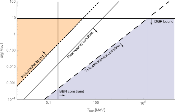
on the normal branch of DGP in order to get the allowed region in parameter space for $\{T_{\text{nuc}},M_{5}\}$ – depicted in Fig.4 (blue shaded region).

It is interesting to compare the thermal entropy of our brane to the holographic bound expected from its surface area in 5D. The entropy for the 5D black hole is $S_{BH}=\frac{A}{4G_{5}}$, while the entropy density in a universe dominated by relativistic particles $s(T)=\frac{4\pi^{2}}{90}g_{*}T_{\text{nuc}}^{3}\simeq 4.71\times T_{\text{nuc}}^{3}$, for $g_{*}=10.75$ effective relativistic degrees of freedom, prior to electron/positron annihilation [32]. This puts a lower bound

$$M_{5}>0.23~{}\bigg{(}\frac{T_{\rm nuc.}}{0.4\,\text{MeV}}\bigg{)}~{}\text{MeV}~{}~{}~{}~{}~{}{\rm(holographic~{}bound)}$$ (5.13)

on the 5D Planck mass $M_{5}=\frac{1}{(32\pi G_{5})^{1\!/3}}$, where $T_{\rm nuc.}$ is the nucleation temperature of the brane. We show the Holographic bound allowed region in parameter space in Fig. 4 (orange shaded region). Eqs. (5.13)-(2.4) constrain the 5D Planck mass to be within 1.5 decades in energy:

$$0.23\,\text{MeV}<M_{5}<9\,\text{MeV},$$ (5.14)

a range that will inevitably shrink with future observations that better constrain BBN, and late-time cosmic expansion history. As we see in Fig.4, the best-fit value for $T_{\rm nuc.}$ from cosmological observations (assuming the thin atmosphere condition) does violate the holographic bound (5.13) by at least 2.5 orders of magnitude, which would decrease the lower limit on $M_{5}$ in Eq. (5.14) by the same factor.

Is this a “show-stopper”? While the holographic bound on entropy remains a very well-motivated conjecture, it is not clear how firm it might be as objects that get close to crossing it are already in the quantum gravity regime where the classical description of spacetime physics fails. One may argue that since the degrees from responsible for thermal entropy of our brane are on scales much smaller than the 5D Planck length, they are not accessible by a 5D bulk observer, and thus are not limited by the 5D holographic bound.

Figure 4: Theoretical and empirical bounds for the Holographic Big Bang model. The DGP bound Eq.(5.12) (thick-black) and the holographic bound Eq.(5.13) (black, thin dashed), together with the BBN bound Eq.(5.11) (vertical black) constitute the theoretical bounds of the model. The top shaded area (orange) is the allowed region for these three bounds to be satisfied. The real velocity bound Eq.(5.8) (thick, grey) and the thin atmosphere condition (5.9) (black, thick dashed) constitute the empirical bounds that HBB must satisfy. The bottom shaded area (blue) is the allowed region of $\{M_{5},T_{\text{nuc}}\}$ parameter space satisfying the empirical bounds, and the arrows indicate the directions in which the different bounds apply. It is clear that the empirical bounds violate the holographic bound for all possible allowed pairs $\{M_{5},T_{\text{nuc}}\}$ by at least 2.5 orders of magnitude. The least severe violation of the holographic bound is for parameters at the bottom left of the plot: for $T_{\text{nuc}}$ being the minimum allowed value by BBN and $M_{5}$ the maximum allowed by the thin atmosphere condition (third column of Table 2).

6 Summary and Discussion

The 5D Holographic Big Bang (HBB) is a novel proposal for a holographic origin of our universe as a 3-brane with induced gravity, out of the collapse of 5D star that can address the traditional problems of big bang cosmology. The main goal of this study was to provide detailed and concrete predictions for this proposal, and to see whether it can serve as a possible competitor to slow-roll inflationary models to explain cosmological observations.

We first focused our attention on a possible mechanism for the nucleation of our 3-brane in which the quantum degrees of freedom of the bulk tunnel into a fuzzball configuration reminiscent to the bubble of nothing model. This mechanism not just provides a possible scenario of brane nucleation but also constrains the Planck mass in the bulk.

Previous work has shown that the presence of uniform thermal gas in the 5D bulk leads a scale-invariant primordial power spectrum for cosmological scalar perturbations. To formalize this result and search for mechanisms that could potentially explain deviations from scale-invariance (observed in the CMB data), we studied cosmological perturbations induced by a thin infalling atmosphere. This atmosphere is composed of a spherically symmetric thermal relativistic gas that the brane encounters after nucleation. We showed that this atmosphere induces a change in the Hubble parameter and also scalar cosmological perturbations on the brane. The power spectrum is scale invariant for large $k$’s and scales as $k$ for small $k$’s.

We then tested this prediction for power spectrum against the cosmological observations. The transition is characterized by a decay of $1/k$ for scales where the power spectrum is highly constrained by data [31] as shown in Fig. 3 (right). We found that our model is broadly consistent with non-parametric reconstruction of primordial power spectrum, but is disfavoured compared to a pure power-law at 2.7$\sigma$ level. We finally outlined various theoretical constraints on the nucleation temperature and 5D Planck mass in the HBB model, and found that the best fit nucleation temperature of the 3-brane was at least 3 orders of magnitude larger than the 5D Planck mass.

This first attempt to understand the detailed consequences of the HBB model for cosmology relies on several simplifying assumptions that can be relaxed in future work. Some of the issues that remain to be tackled are:

1. Perhaps our most perplexing finding was that our best-fit model violated the holographic entropy bound by 8 orders of magnitude. It is not yet clear whether this is a feature or a bug!

2. It would be interesting to study how brane cosmological perturbations will be affected by the large-scale curvature of the bulk (in a 5D Schwarzschild of Kerr spacetime).

3. Other observables that remain to be computed are the amplitude of tensor modes and the non-gaussianity, although we do not expect them to be significant.

4. Given that the speed of sound for a relativistic 5D atmosphere is $c_{s}=c/2$, one expect ${\cal O}(0.2)$ relativistic corrections to the atmosphere profile, which we have ignored. This could affect the functional shape of the power spectrum at a similar level, potentially improving (or worsening) the fit to the data. A related issue is whether the hydrostatic equilibrium profile for the relativistic thin atmosphere is stable.

To conclude, while we believe the 5D holographic big bang remains an intriguing possibility for the origin of our universe, there remain empirical and theoretical challenges to its status amongst various scenarios for the early universe cosmology that should be addressed in future work.

Appendix A Inhomogeneous Cosmological perturbations on the bulk

If we consider the metric (3.24) and homogeneous perturbations of the form (3.25) the induced metric on the brane is $\gamma_{\mu\nu}=g_{\alpha\beta}e^{\alpha}_{\mu}e^{\beta}_{\nu}$ that to first order in $\epsilon$ reads:

$$ds^{2}_{\text{brane}}=[(f_{0}^{\prime 2}-1)-2\epsilon\left(\text{$\hat{\hat{\Psi}}_{5}^{0}$}(f)f_{0}^{\prime 2}+\text{$\hat{\Phi}_{5}^{0}$}(f)\right)]dt^{2}+[1-2\epsilon\text{$\hat{\Psi}_{5}^{0}$}(f)][dx^{2}+dy^{2}+dz^{2}]\,,$$ (A.1)

where $f^{\prime}=\frac{\text{d}f}{\text{d}t}$. The induced metric on the brane has to be able to describe a Friedmann universe for which we make the following identifications

$$-d\tau^{2}=[(f_{0}^{\prime 2}-1)-2\epsilon\left(\hat{\Psi}_{5}^{0}f_{0}^{\prime 2}+\hat{\Phi}_{5}^{0}\right)]dt^{2}\,,\quad a^{2}=[1-2\epsilon\hat{\Psi}_{5}^{0}]\,,$$ (A.2)

where $\tau$ is the proper time of the brane and $a$ is the scale factor. On top of the homogeneous perturbations we are now going to consider anisotropies

$$\Phi_{5}=\epsilon\Phi_{5}^{0}(w)+\epsilon_{1}\Phi_{5}^{1}(x^{\alpha})\,,\quad\Psi_{5}=\epsilon\Psi_{5}^{0}(w)+\epsilon_{1}\Psi_{5}^{1}(x^{\alpha})\,,\quad f=f_{0}(t)+\epsilon_{1}f_{1}(x^{\alpha})\,,$$ (A.3)

where $\epsilon_{1}\ll 1$ is a parameter that controls the anisotropic perturbations and $\epsilon\epsilon_{1}\ll\epsilon,\epsilon_{1}$. The induced metric can be written as

$$ds^{2}_{\text{brane}}=-[1+\frac{2\epsilon_{1}}{f_{0}^{\prime 2}-1}(\hat{\Phi}_{5}^{1}+\hat{\Psi}_{5}^{1}f_{0}^{2}-f_{0}^{\prime}f_{1}^{\prime})]d\tau^{2}+2a\epsilon_{1}\frac{f_{0}^{\prime}f_{1,i}}{\sqrt{f_{0}^{\prime 2}-1}}dx^{i}d\tau+a^{2}(1-2\hat{\Psi}_{5}^{1}\epsilon_{1})dx^{2}\,,$$ (A.4)

where $\hat{\Psi}_{5}=\Psi_{5}(w=f(x^{\mu}))$ are the metric functions projected to the brane. The general form of a 4D metric including scalar and vector cosmological perturbation in 4D are that contains all the terms in Eq. (A.4)

$$ds^{2}_{\text{brane}}=-(1+2\phi_{4})d\tau^{2}-2aB_{i}d\tau dx^{i}+a^{2}(1-2\psi_{4})dx^{2}\,,$$ (A.5)

and thus we identify

$$\phi_{4}=\frac{\epsilon_{1}}{f_{0}^{\prime 2}-1}(\hat{\Phi}_{5}^{1}+\hat{\Psi}_{5}^{1}f_{0}^{2}-f_{0}^{\prime}f_{1}^{\prime})\,,\quad\psi_{4}=\hat{\Psi}_{5}^{1}\epsilon_{1}\,,\quad B_{i}=\epsilon_{1}\frac{f_{0}^{\prime}f_{1,i}}{\sqrt{f_{0}^{\prime 2}-1}}\,.$$ (A.6)

Note that the Newtonian gauge on the bulk does not translate into a Newtonian gauge on the brane and that some perturbations that are scalars in 5D are projected as a vectorial perturbation component in 4D. The scalar gauge invariant quantities can be constructed from Eq.(A.4) as

$$\Phi_{4} = \phi_{4}-\partial_{\tau}(aB)\,,$$ (A.7)

$$\Psi_{4} = \psi_{4}+HaB\,,$$ (A.8)

where, $H$ is the Hubble constant and $B$ is the scalar part of the vector metric perturbation $B_{i}$. From our construction the Hubble constant is

$$H=\frac{\dot{a}}{a}=-\frac{\epsilon\hat{\Psi}_{5}^{0}}{a^{2}}\,,$$ (A.9)

and thus Eq.(A.8) reduces to $\Psi_{4}=\psi_{4}$ to first order in $\epsilon,\epsilon_{1}$.

Appendix B Derivation of the power spectrum

With use of the Poisson equation in 4D

$$\nabla^{2}\Psi_{5}(y)=\frac{8\pi G_{5}}{3}\rho_{5}(y)\,,$$ (B.1)

and the expression for the energy density correlation function

$$\left\langle\rho_{5}(y_{1})\rho_{5}(y_{2})\right\rangle\simeq\alpha(T_{5})^{6}\delta^{4}(y_{1}-y_{2})\,,$$ (B.2)

we can write the 2-point correlation function of $\Psi_{5}$ using the Green’s function for the Laplacian operator

$$\langle\Psi_{5}(x_{1})\Psi_{5}(x_{2})\rangle=\alpha\bigg{(}\frac{8\pi G_{5}}{3}\bigg{)}^{2}\bigg{(}\frac{1}{4\pi^{2}}\bigg{)}^{2}\int d^{4}y\frac{(T_{5}(y))^{6}}{|y-x_{1}|^{2}|y-x_{2}|^{2}}\,.$$ (B.3)

The junction condition between the 5D and 4D metrics (3.24) and (A.1) allow us to compute $\langle\Psi_{4}({\bf{x}_{1}})\Psi_{4}({\bf{x}_{2}})\rangle$

$$\langle\Psi_{4}({\bf{x}_{1}})\Psi_{4}({\bf{x}_{2}})\rangle = \langle\Psi_{5}({\bf{x}_{1}},x_{1w}=0)\Psi_{4}({\bf{x}_{2}},x_{2w}=0)\rangle$$ (B.4)

$$= \alpha\bigg{(}\frac{2G_{5}}{3\pi}\bigg{)}^{2}\!\!\!\int d^{3}{\bf{y}_{3}}dy_{w}\frac{(T_{5}(y_{w}))^{6}}{(|{\bf{x}_{1}}-{\bf{y}_{3}}|^{2}+|y_{w}|^{2})(|{\bf{x}_{2}}-{\bf{y}_{3}}|^{2}+|y_{w}|^{2})}$$

where we have decomposed the bulk coordinate as $y=({\bf{y}_{3}},y_{w})$ and we have set the temperature to be just a function of the $w$ direction of the bulk. Combining expressions (4.3), (4.4), (B.4) and setting ${\bf{x}_{1}}=0$ we have

$$P_{\zeta}(k) = \alpha\bigg{(}\frac{2G_{5}}{3\pi\,\Delta\text{ln}H}\bigg{)}^{2}\int\frac{d^{3}{\bf{y}_{3}}\,dy_{w}\,(T_{5}(y_{w}))^{6}}{|{\bf{y}_{3}}|^{2}+|y_{w}|^{2}}\int d^{3}x\frac{e^{i{\bf{k\cdot x}}}}{|{\bf{x}}-{\bf{y}_{3}}|^{2}+|y_{w}|^{2}}\,,$$ (B.5)

$$= \alpha\bigg{(}\frac{2G_{5}}{3\pi\,\Delta\text{ln}H}\bigg{)}^{2}\int\frac{d^{3}{\bf{y}_{3}}\,dy_{w}\,(T_{5}(y_{w}))^{6}}{|{\bf{y}_{3}}|^{2}+|y_{w}|^{2}}\int d^{3}{\bf{x}}^{\prime}\frac{e^{i{\bf{k\cdot x^{\prime}}}}e^{i{\bf{k\cdot{\bf{y}_{3}}}}}}{|{\bf{x}}^{\prime}|^{2}+|y_{w}|^{2}}\,,$$

$$= \alpha\bigg{(}\frac{2G_{5}}{3\pi\,\Delta\text{ln}H}\bigg{)}^{2}\int dy_{w}\,(T_{5}(y_{w}))^{6}\bigg{(}\int d^{3}{\bf{x}}^{\prime}\frac{e^{i{\bf{k\cdot x^{\prime}}}}}{|{\bf{x}}^{\prime}|^{2}+|y_{w}|^{2}}\bigg{)}^{2}\,,$$

$$= \alpha\bigg{(}\frac{2G_{5}}{3\pi\,\Delta\text{ln}H}\bigg{)}^{2}\frac{1}{(4\pi k)^{2}}\int dy_{w}\,e^{-2|y_{w}|k}\,(T_{5}(y_{w}))^{6}\,,$$

where we have performed the coordinate transformation ${\bf{x}}^{\prime}={\bf{x}}-{\bf{y}_{3}}$, and use the result $\int\frac{d^{3}x\,e^{i{\bf{k\cdot x}}}}{|x|^{2}+|m|^{2}}=\frac{e^{-k|m|}}{4\pi k}$.

With this we are able to write

$${\cal{P}}(k)=\frac{k^{3}}{2\pi^{2}}P_{\zeta}(k)=\beta\,k\int_{0}^{\infty}dw\,e^{-2|w|k}\,(T_{5}(w))^{6}\,,$$ (B.6)

where $\beta=\frac{\alpha}{2}\bigg{(}\!\frac{G_{5}}{6\Delta\text{ln}H\,\pi^{3}}\!\bigg{)}^{2}$. Note that we are in integrating between $[0,\infty)$ because of the $\mathbb{Z}_{2}$ symmetry. Because the temperature profile is analytic it admits a Taylor expansion of the form

$$(T_{5}(w))^{6}=\sum_{n=0}^{\infty}\frac{T^{6^{(n)}}(0,\bar{\gamma},\bar{w})}{n!}w^{n}\,,$$ (B.7)

and thus the power spectrum Eq.(B.6) admits a series decomposition of the form

$${\cal{P}}(k)=\beta\sum_{n=0}^{\infty}\frac{T^{6^{(n)}}(0,\bar{\gamma},\bar{w})}{k^{n}}2^{-1-n}\,.$$ (B.8)

This last expression implies that for large $k$ the correction to a scale invariant power spectrum goes as $1/k$. If the integral in Eq.(B.6) is performed in the rage $(-\infty,\infty)$ the the power spectrum series would be

$${\cal{P}}(k)=\beta\sum_{n=0}^{\infty}\frac{T^{6^{(2n)}}(0,\bar{\gamma},\bar{w})}{k^{2n}}2^{-1-2n}\,,$$ (B.9)

giving a correction from scale invariant that goes as $1/k^{2}$ for large $k$. This correction renders model disfavourable in comparison with the symmetric case, where we have a $1/k$ decay. This is the reason why we work with the symmetric integral Eq.(B.6).

References

- [1] Planck Collaboration, P. A. R. Ade et. al., Planck 2015 results. XIII. Cosmological parameters, arXiv:1502.0158.
- [2] R. Pourhasan, N. Afshordi, and R. B. Mann, Out of the White Hole: A Holographic Origin for the Big Bang, JCAP 1404 (2014) 005, [arXiv:1309.1487].
- [3] G. R. Dvali, G. Gabadadze, and M. Porrati, 4-D gravity on a brane in 5-D Minkowski space, Phys. Lett. B485 (2000) 208–214, [hep-th/0005016].
- [4] R. Gregory, N. Kaloper, R. C. Myers, and A. Padilla, A New perspective on DGP gravity, JHEP 10 (2007) 069, [arXiv:0707.2666].
- [5] S. D. Mathur, Tunneling into fuzzball states, Gen. Rel. Grav. 42 (2010) 113–118, [arXiv:0805.3716].
- [6] E. Witten, Instability of the kaluza-klein vacuum, Nuclear Physics B 195 (1982), no. 3 481 – 492.
- [7] O. Lunin and S. D. Mathur, Statistical interpretation of Bekenstein entropy for systems with a stretched horizon, Phys. Rev. Lett. 88 (2002) 211303, [hep-th/0202072].
- [8] M. Pospelov and J. Pradler, Big Bang Nucleosynthesis as a Probe of New Physics, Ann. Rev. Nucl. Part. Sci. 60 (2010) 539–568, [arXiv:1011.1054].
- [9] T. Azizi, M. Sadegh Movahed, and K. Nozari, Observational Constraints on the Normal Branch of a Warped DGP Cosmology, New Astron. 17 (2012) 424–432, [arXiv:1111.3195].
- [10] Planck Collaboration, P. A. R. Ade et. al., Planck 2015 results. XIV. Dark energy and modified gravity, arXiv:1502.0159.
- [11] U. Seljak and M. Zaldarriaga, A Line-of-Sight Integration Approach to Cosmic Microwave Background Anisotropies, The Astrophysical Journal 469 (Oct., 1996) 437, [astro-ph/9603033].
- [12] M. Zaldarriaga, U. Seljak, and E. Bertschinger, Integral Solution for the Microwave Background Anisotropies in Nonflat Universes, The Astrophysical Journal 494 (Feb., 1998) 491–502, [astro-ph/9704265].
- [13] A. Lewis and S. Bridle, Cosmological parameters from CMB and other data: A Monte Carlo approach, Phys. Rev. D 66 (Nov., 2002) 103511, [astro-ph/0205436].
- [14] A. Lewis, A. Challinor, and A. Lasenby, Efficient Computation of Cosmic Microwave Background Anisotropies in Closed Friedmann-Robertson-Walker Models, The Astrophysical Journal 538 (Aug., 2000) 473–476, [astro-ph/9911177].
- [15] C. Howlett, A. Lewis, A. Hall, and A. Challinor, CMB power spectrum parameter degeneracies in the era of precision cosmology, JCAP 4 (Apr., 2012) 027, [arXiv:1201.3654].
- [16] A. Lewis, Efficient sampling of fast and slow cosmological parameters, Phys. Rev. D 87 (May, 2013) 103529, [arXiv:1304.4473].
- [17] A. Lewis, CAMB Notes, http://cosmologist.info/notes/CAMB.pdf.
- [18] F. Beutler, C. Blake, M. Colless, D. H. Jones, L. Staveley-Smith, L. Campbell, Q. Parker, W. Saunders, and F. Watson, The 6dF Galaxy Survey: baryon acoustic oscillations and the local Hubble constant, mnras 416 (Oct., 2011) 3017–3032, [arXiv:1106.3366].
- [19] C. Blake and others., The WiggleZ Dark Energy Survey: mapping the distance-redshift relation with baryon acoustic oscillations, mnras 418 (Dec., 2011) 1707–1724, [arXiv:1108.2635].
- [20] L. Anderson et. al., The clustering of galaxies in the SDSS-III Baryon Oscillation Spectroscopic Survey: baryon acoustic oscillations in the Data Release 9 spectroscopic galaxy sample, mnras 427 (Dec., 2012) 3435–3467, [arXiv:1203.6594].
- [21] F. Beutler, C. Blake, M. Colless, D. H. Jones, L. Staveley-Smith, G. B. Poole, L. Campbell, Q. Parker, W. Saunders, and F. Watson, The 6dF Galaxy Survey: z 0 measurements of the growth rate and 8, mnras 423 (July, 2012) 3430–3444, [arXiv:1204.4725].
- [22] N. Padmanabhan, X. Xu, D. J. Eisenstein, R. Scalzo, A. J. Cuesta, K. T. Mehta, and E. Kazin, A 2 per cent distance to z = 0.35 by reconstructing baryon acoustic oscillations - I. Methods and application to the Sloan Digital Sky Survey, mnras 427 (Dec., 2012) 2132–2145, [arXiv:1202.0090].
- [23] L. Anderson and others., The clustering of galaxies in the SDSS-III Baryon Oscillation Spectroscopic Survey: baryon acoustic oscillations in the Data Releases 10 and 11 Galaxy samples, mnras 441 (June, 2014) 24–62, [arXiv:1312.4877].
- [24] L. Samushia and others., The clustering of galaxies in the SDSS-III Baryon Oscillation Spectroscopic Survey: measuring growth rate and geometry with anisotropic clustering, mnras 439 (Apr., 2014) 3504–3519, [arXiv:1312.4899].
- [25] A. J. Ross, L. Samushia, C. Howlett, W. J. Percival, A. Burden, and M. Manera, The clustering of the SDSS DR7 main Galaxy sample - I. A 4 per cent distance measure at z = 0.15, mnras 449 (May, 2015) 835–847, [arXiv:1409.3242].
- [26] Planck Collaboration, P. A. R. Ade et. al., Planck 2015 results. XV. Gravitational lensing, Astron. Astrophys. 594 (2016) A15, [arXiv:1502.0159].
- [27] Planck Collaboration, N. Aghanim et. al., Planck 2015 results. XI. CMB power spectra, likelihoods, and robustness of parameters, Astron. Astrophys. (2015) [arXiv:1507.0270].
- [28] Planck Collaboration, P. A. R. Ade et. al., Planck 2015 results. XXIV. Cosmology from Sunyaev-Zeldovich cluster counts, Astron. Astrophys. 594 (2016) A24, [arXiv:1502.0159].
- [29] C. L. Reichardt et. al., A Measurement of Secondary Cosmic Microwave Background Anisotropies with Two Years of South Pole Telescope Observations, apj 755 (Aug., 2012) 70, [arXiv:1111.0932].
- [30] S. Das et. al., The Atacama Cosmology Telescope: temperature and gravitational lensing power spectrum measurements from three seasons of data, jcap 4 (Apr., 2014) 014, [arXiv:1301.1037].
- [31] Planck Collaboration, P. A. R. Ade et. al., Planck 2015 results. XX. Constraints on inflation, arXiv:1502.0211.
- [32] E. W. Kolb and M. S. Turner, The early universe. 1990.