Global and Local Multiple SLEs for $\kappa\leq 4$ and
Connection Probabilities for Level Lines of GFF

Abstract

This article pertains to the classification of multiple Schramm-Loewner evolutions ($\operatorname{SLE}$). We construct the pure partition functions of multiple $\operatorname{SLE}_{\kappa}$ with $\kappa\in(0,4]$ and relate them to certain extremal multiple $\operatorname{SLE}$ measures, thus verifying a conjecture from [BBK05, KP16]. We prove that the two approaches to construct multiple $\operatorname{SLE}$s — the global, configurational construction of [KL07, Law09a] and the local, growth process construction of [BBK05, Dub07, Gra07, KP16] — agree.

The pure partition functions are closely related to crossing probabilities in critical statistical mechanics models. With explicit formulas in the special case of $\kappa=4$, we show that these functions give the connection probabilities for the level lines of the Gaussian free field ($\operatorname{GFF}$) with alternating boundary data. We also show that certain functions, known as conformal blocks, give rise to multiple $\operatorname{SLE}_{4}$ that can be naturally coupled with the $\operatorname{GFF}$ with appropriate boundary data.

1 Introduction

Conformal invariance and critical phenomena in two-dimensional statistical physics have been active areas of research in the last few decades, both in the mathematics and physics communities. Conformal invariance can be studied in terms of correlations and interfaces in critical models. This article concerns conformally invariant probability measures on curves that describe scaling limits of interfaces in critical lattice models (with suitable boundary conditions).

For one chordal curve between two boundary points, such scaling limit results have been rigorously established for many models: critical percolation [Smi01, CN07], the loop-erased random walk and the uniform spanning tree [LSW04, Zha08b], level lines of the discrete Gaussian free field [SS09, SS13], and the critical Ising and FK-Ising models [CDCH⁺14]. In this case, the limiting object is a random curve known as the chordal $\operatorname{SLE}_{\kappa}$ (Schramm-Loewner evolution), uniquely characterized by a single parameter $\kappa\geq 0$ together with conformal invariance and a domain Markov property [Sch00]. In general, interfaces of critical lattice models with suitable boundary conditions converge to variants of the $\operatorname{SLE}_{\kappa}$ (see, e.g., [HK13] for the critical Ising model with plus-minus-free boundary conditions, and [Zha08b] for the loop-erased random walk). In particular, multiple interfaces converge to several interacting $\operatorname{SLE}$ curves [Izy17, Wu17, BPW18, KS18]. These interacting random curves cannot be classified by conformal invariance and the domain Markov property alone, but additional data is needed [BBK05, Dub07, Gra07, KL07, Law09a, KP16]. Together with results in [BPW18], the main results of the present article provide with a general classification for $\kappa\leq 4$.

It is also natural to ask questions about the global behavior of the interfaces, such as their crossing or connection probabilities. In fact, such a crossing probability, known as Cardy’s formula, was a crucial ingredient in the proof of the conformal invariance of the scaling limit of critical percolation [Smi01, CN07]. In Figure 1.1, a simulation of the critical Ising model with alternating boundary conditions is depicted. The figure shows one possible connectivity of the interfaces separating the black and yellow regions, but when sampling from the Gibbs measure, other planar connectivities can also arise. One may then ask with which probability do the various connectivities occur. For discrete models, the answer is known only for loop-erased random walks ($\kappa=2$) and the double-dimer model ($\kappa=4$) [KW11a, KKP17], whereas for instance the cases of the Ising model ($\kappa=3$) and percolation ($\kappa=6$) are unknown. However, scaling limits of these connection probabilities are encoded in certain quantities related to multiple $\operatorname{SLE}$s, known as pure partition functions [PW18]. These functions give the Radon-Nikodym derivatives of multiple $\operatorname{SLE}$ measures with respect to product measures of independent $\operatorname{SLE}$s.

In this article, we construct the pure partition functions of multiple $\operatorname{SLE}_{\kappa}$ for all $\kappa\in(0,4]$ and show that they are smooth, positive, and (essentially) unique. We also relate these functions to certain extremal multiple $\operatorname{SLE}$ measures, thus verifying a conjecture from [BBK05, KP16]. To find the pure partition functions, we give a global construction of multiple $\operatorname{SLE}_{\kappa}$ measures in the spirit of [KL07, Law09a, Law09b], but pertaining to the complete classification of these random curves. We also prove that, as probability measures on curve segments, these “global” multiple $\operatorname{SLE}$s agree with another approach to construct and classify interacting $\operatorname{SLE}$ curves, known as “local” multiple $\operatorname{SLE}$s [BBK05, Dub07, Gra07, KP16].

The $\operatorname{SLE}_{4}$ processes are known to be realized as level lines of the Gaussian free field ($\operatorname{GFF}$). In the spirit of [KW11a, KKP17], we find algebraic formulas for the pure partition functions in this case and show that they give explicitly the connection probabilities for the level lines of the $\operatorname{GFF}$ with alternating boundary data. We also show that certain functions, known as conformal blocks, give rise to multiple $\operatorname{SLE}_{4}$ processes that can be naturally coupled with the $\operatorname{GFF}$ with appropriate boundary data.

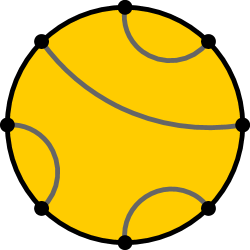
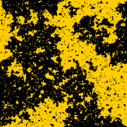
Figure 1.1: Simulation of the critical Ising model with alternating boundary conditions and the corresponding link pattern $\alpha\in\mathrm{LP}_{4}$.

1.1 Multiple SLEs and Pure Partition Functions

One can naturally view interfaces in discrete models as dynamical processes. Indeed, in his seminal article [Sch00], O. Schramm defined the $\operatorname{SLE}_{\kappa}$ as a random growth process (Loewner chain) whose time evolution is encoded in an ordinary differential equation (Loewner equation, see Section 2.1). Using the same idea, one may generate processes of several $\operatorname{SLE}_{\kappa}$ curves by describing their time evolution via a Loewner chain. Such processes are local multiple $\operatorname{SLE}$s: probability measures on curve segments growing from $2N$ fixed boundary points $x_{1},\ldots,x_{2N}\in\partial\Omega$ of a simply connected domain $\Omega\subset\mathbb{C}$, only defined up to a stopping time strictly smaller than the time when the curves touch (we call this localization).

We prove in Theorem 1.3 that, when $\kappa\leq 4$, localizations of global multiple $\operatorname{SLE}$s give rise to local multiple $\operatorname{SLE}$s. Then, the $2N$ curve segments form $N$ planar, non-intersecting simple curves connecting the $2N$ marked boundary points pairwise, as in Figure 1.1 for the critical Ising interfaces. Topologically, these $N$ curves form a planar pair partition, which we call a link pattern and denote by $\alpha=\{\{a_{1},b_{1}\},\ldots,\{a_{N},b_{N}\}\}$, where $\{a,b\}$ are the pairs in $\alpha$, called links. The set of link patterns of $N$ links on $\{1,2,\ldots,2N\}$ is denoted by $\mathrm{LP}_{N}$. The number of elements in $\mathrm{LP}_{N}$ is a Catalan number, $\#\mathrm{LP}_{N}=\mathrm{C}_{N}=\frac{1}{N+1}\binom{2N}{N}$. We also denote by $\mathrm{LP}=\bigsqcup_{N\geq 0}\mathrm{LP}_{N}$ the set of link patterns of any number of links, where we include the empty link pattern $\emptyset\in\mathrm{LP}_{0}$ in the case $N=0$.

By the results of [Dub07, KP16], the local $N$-$\operatorname{SLE}_{\kappa}$ probability measures are classified by smooth functions $\mathcal{Z}$ of the marked points, called partition functions. It is believed that they form a $\mathrm{C}_{N}$-dimensional space, with basis given by certain special elements $\mathcal{Z}_{\alpha}$, called pure partition functions, indexed by the $\mathrm{C}_{N}$ link patterns $\alpha\in\mathrm{LP}_{N}$. These functions can be related to scaling limits of crossing probabilities in discrete models — see [KKP17, PW18] and Section 1.4 below for discussions on this. In general, however, even the existence of such functions $\mathcal{Z}_{\alpha}$ is not clear. We settle this problem for all $\kappa\in(0,4]$ in Theorem 1.1.

To state our results, we need to introduce some definitions and notation. Throughout this article, we denote by $\mathbb{H}=\{z\in\mathbb{C}\colon\operatorname{Im}(z)>0\}$ the upper half-plane, and we use the following real parameters: $\kappa>0$,

$$h=\frac{6-\kappa}{2\kappa},\qquad\qquad\text{and}\qquad\qquad c=\frac{(3\kappa-8)(6-\kappa)}{2\kappa}.$$

A multiple $\operatorname{SLE}_{\kappa}$ partition function is a positive smooth function

$$\mathcal{Z}\colon\mathfrak{X}_{2N}\to\mathbb{R}_{>0}$$

defined on the configuration space $\mathfrak{X}_{2N}:=\;\{(x_{1},\ldots,x_{2N})\in\mathbb{R}^{2N}\colon x_{1}<\cdots<x_{2N}\}$ satisfying the following two properties:

• Partial differential equations of second order: We have

  $$\left[\frac{\kappa}{2}\partial^{2}_{i}+\sum_{j\neq i}\left(\frac{2}{x_{j}-x_{i}}\partial_{j}-\frac{2h}{(x_{j}-x_{i})^{2}}\right)\right]\mathcal{Z}(x_{1},\ldots,x_{2N})=0,\qquad\text{for all }i\in\{1,\ldots,2N\}.$$ (1.1)

• Möbius covariance: For all Möbius maps $\varphi$ of $\mathbb{H}$ such that $\varphi(x_{1})<\cdots<\varphi(x_{2N})$, we have

  $$\mathcal{Z}(x_{1},\ldots,x_{2N})=\prod_{i=1}^{2N}\varphi^{\prime}(x_{i})^{h}\times\mathcal{Z}(\varphi(x_{1}),\ldots,\varphi(x_{2N})).$$ (1.2)

Given such a function, one can construct a local $N$-$\operatorname{SLE}_{\kappa}$ as we discuss in Section 4.2. The above properties $\mathrm{(PDE)}$ (1.1) and $\mathrm{(COV)}$ (1.2) guarantee that this local multiple $\operatorname{SLE}$ process is conformally invariant, the marginal law of one curve with respect to the joint law of all of the curves is a suitably weighted chordal $\operatorname{SLE}_{\kappa}$, and that the curves enjoy a certain “commutation”, or “stochastic reparameterization invariance” property — see [Dub07, Gra07, KP16] for details.

The pure partition functions $\mathcal{Z}_{\alpha}\colon\mathfrak{X}_{2N}\to\mathbb{R}_{>0}$ are indexed by link patterns $\alpha\in\mathrm{LP}_{N}$. They are positive solutions to $\mathrm{(PDE)}$ (1.1) and $\mathrm{(COV)}$ (1.2) singled out by boundary conditions given in terms of their asymptotic behavior, determined by the link pattern $\alpha$:

• Asymptotics: For all $\alpha\in\mathrm{LP}_{N}$ and for all $j\in\{1,\ldots,2N-1\}$ and $\xi\in(x_{j-1},x_{j+2})$, we have

  $$\lim_{x_{j},x_{j+1}\to\xi}\frac{\mathcal{Z}_{\alpha}(x_{1},\ldots,x_{2N})}{(x_{j+1}-x_{j})^{-2h}}=\begin{cases}0,\quad&\text{if }\{j,j+1\}\notin\alpha,\\ \mathcal{Z}_{\hat{\alpha}}(x_{1},\ldots,x_{j-1},x_{j+2},\ldots,x_{2N}),&\text{if }\{j,j+1\}\in\alpha,\end{cases}$$ (1.3)

  where $\hat{\alpha}=\alpha/\{j,j+1\}\in\mathrm{LP}_{N-1}$ denotes the link pattern obtained from $\alpha$ by removing the link $\{j,j+1\}$ and relabeling the remaining indices by $1,2,\ldots,2N-2$ (see Figure 1.2).

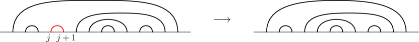
Figure 1.2: The removal of a link from a link pattern (here $j=4$ and $N=7$). The left figure is the link pattern $\alpha=\{\{1,14\},\{2,3\},\{4,5\},\{6,13\},\{7,10\},\{8,9\},\{11,12\}\}\in\mathrm{LP}_{7}$ and the right figure the link pattern $\alpha/\{4,5\}=\{\{1,12\},\{2,3\},\{4,11\},\{5,8\},\{6,7\},\{9,10\}\}\in\mathrm{LP}_{6}$.

Attempts to find and classify these functions using Coulomb gas techniques have been made, e.g., in [BBK05, Dub06, Dub07, FK15d, KP16]; see also [DF85, FSK15, FSKZ17, LV17, LV18]. The main difficulty in the Coulomb gas approach is to show that the constructed functions are positive, whereas smoothness is immediate. On the other hand, as we will see in Lemma 4.1, positivity is manifest from the global construction of multiple $\operatorname{SLE}$s, but in this approach, the main obstacle is establishing the smoothness. In this article, we combine the approach of [KL07, Law09a] (global construction) with that of [Dub07, Dub15a, Dub15b, KP16] (local construction and PDE approach), to show that there exist unique pure partition functions for multiple $\operatorname{SLE}_{\kappa}$ for all $\kappa\in(0,4]$:

Theorem 1.1.

Let $\kappa\in(0,4]$. There exists a unique collection $\{\mathcal{Z}_{\alpha}\colon\alpha\in\mathrm{LP}\}$ of smooth functions $\mathcal{Z}_{\alpha}\colon\mathfrak{X}_{2N}\to\mathbb{R}$, for $\alpha\in\mathrm{LP}_{N}$, satisfying the normalization $\mathcal{Z}_{\emptyset}=1$, the power law growth bound given in (2.4) in Section 2, and properties $\mathrm{(PDE)}$ (1.1), $\mathrm{(COV)}$ (1.2), and $\mathrm{(ASY)}$ (1.3). These functions have the following further properties:

1. For all $\alpha\in\mathrm{LP}_{N}$, we have the stronger power law bound

   $$0<\mathcal{Z}_{\alpha}(x_{1},\ldots,x_{2N})\leq\prod_{\{a,b\}\in\alpha}|x_{b}-x_{a}|^{-2h}.$$ (1.4)

2. For each $N\geq 0$, the functions $\{\mathcal{Z}_{\alpha}\colon\alpha\in\mathrm{LP}_{N}\}$ are linearly independent.

Next, we make some remarks concerning the above result.

• The bound (1.4) stated above is very strong. First of all, together with smoothness, the positivity in (1.4) enables us to construct local multiple $\operatorname{SLE}$s (Corollary 1.2). Second, using the upper bound in (1.4), we will prove in Proposition 4.9 that the curves in these local multiple $\operatorname{SLE}$s are continuous up to and including the continuation threshold, and they connect the marked points in the expected way — according to the connectivity $\alpha$. Third, the upper bound in (1.4) is also crucial in our proof of Theorem 1.4, stated below, concerning the connection probabilities of the level lines of the $\operatorname{GFF}$, as well as for establishing analogous results for other models [PW18].

• For $\kappa=2$, the existence of the functions $\mathcal{Z}_{\alpha}$ was already known before [KL05, KKP17]. In this case, the positivity and smoothness can be established by identifying $\mathcal{Z}_{\alpha}$ as scaling limits of connection probabilities for multichordal loop-erased random walks.

• In general, it follows from Theorem 1.1 that the functions $\mathcal{Z}_{\alpha}$ constructed in the previous works [FK15a, KP16] are indeed positive, as conjectured, and agree with the functions of Theorem 1.1.

• Above, the pure partition functions $\mathcal{Z}_{\alpha}$ are only defined for the upper half-plane $\mathbb{H}$. In other simply connected domains $\Omega$, when the marked points lie on sufficiently smooth boundary segments, we may extend the definition of $\mathcal{Z}_{\alpha}$ by conformal covariance: taking any conformal map $\varphi\colon\Omega\to\mathbb{H}$ such that $\varphi(x_{1})<\cdots<\varphi(x_{2N})$, we set

  $$\mathcal{Z}_{\alpha}(\Omega;x_{1},\ldots,x_{2N}):=\prod_{i=1}^{2N}|\varphi^{\prime}(x_{i})|^{h}\times\mathcal{Z}_{\alpha}(\varphi(x_{1}),\ldots,\varphi(x_{2N})).$$ (1.5)

Both the global and local definitions of multiple $\operatorname{SLE}$s enjoy conformal invariance and a domain Markov property. However, only in the case of one curve, these two properties uniquely determine the $\operatorname{SLE}_{\kappa}$. With $N\geq 2$, configurations of curves connecting the marked points $x_{1},\ldots,x_{2N}\in\partial\Omega$ in the simply connected domain $\Omega$ have non-trivial conformal moduli, and their probability measures should form a convex set of dimension higher than one. The classification of local multiple $\operatorname{SLE}$s is well established: they are in one-to-one correspondence with (normalized) partition functions [Dub07, KP16]. Thus, we may characterize the convex set of these local $N$-$\operatorname{SLE}_{\kappa}$ probability measures in the following way:

Corollary 1.2.

Let $\kappa\in(0,4]$. For any $\alpha\in\mathrm{LP}_{N}$, there exists a local $N$-$\operatorname{SLE}_{\kappa}$ with partition function $\mathcal{Z}_{\alpha}$. For any $N\geq 1$, the convex hull of the local $N$-$\operatorname{SLE}_{\kappa}$ corresponding to $\{\mathcal{Z}_{\alpha}\colon\alpha\in\mathrm{LP}_{N}\}$ has dimension $\mathrm{C}_{N}-1$. The $\mathrm{C}_{N}$ local $N$-$\operatorname{SLE}_{\kappa}$ probability measures with pure partition functions $\mathcal{Z}_{\alpha}$ are the extremal points of this convex set.

1.2 Global Multiple SLEs

To prove Theorem 1.1, we construct the pure partition functions $\mathcal{Z}_{\alpha}$ from the Radon-Nikodym derivatives of global multiple $\operatorname{SLE}$ measures with respect to product measures of independent $\operatorname{SLE}$s. To this end, in Theorem 1.3, we give a construction of global multiple $\operatorname{SLE}_{\kappa}$ measures, for any number of curves and for all possible topological connectivities, when $\kappa\in(0,4]$. The construction is not new as such: it was done by M. Kozdron and G. Lawler [KL07] in the special case of the rainbow link pattern $\boldsymbol{\underline{\Cap}}_{N}$, illustrated in Figure 3.1 (see also [Dub06, Section 3.4]). For general link patterns, an idea for the construction appeared in [Law09a, Section 2.7]. However, to prove local commutation of the curves, one needs sufficient regularity that was not established in these articles (for this, see [Dub07, Dub15a, Dub15b]).

In the previous works [KL07, Law09a], the global multiple $\operatorname{SLE}$s were defined in terms of Girsanov re-weighting of chordal $\operatorname{SLE}$s. We prefer another definition, where only a minimal amount of characterizing properties are given. In subsequent work [BPW18], we prove that this definition is optimal in the sense that the global multiple $\operatorname{SLE}$s are uniquely determined by the below stated conditional law property.

First, we define a (topological) polygon to be a $(2N+1)$-tuple $(\Omega;x_{1},\ldots,x_{2N})$, where $\Omega\subset\mathbb{C}$ is a simply connected domain and $x_{1},\ldots,x_{2N}\in\partial\Omega$ are $2N$ distinct boundary points appearing in counterclockwise order on locally connected boundary segments. We also say that $U\subset\Omega$ is a sub-polygon of $\Omega$ if $U$ is simply connected and $U$ and $\Omega$ agree in neighborhoods of $x_{1},\ldots,x_{2N}$. When $N=1$, we let $X_{0}(\Omega;x_{1},x_{2})$ be the set of continuous simple unparameterized curves in $\Omega$ connecting $x_{1}$ and $x_{2}$ such that they only touch the boundary $\partial\Omega$ in $\{x_{1},x_{2}\}$. More generally, when $N\geq 2$, we consider pairwise disjoint continuous simple curves in $\Omega$ such that each of them connects two points among $\{x_{1},\ldots,x_{2N}\}$. We encode the connectivities of the curves in link patterns $\alpha=\{\{a_{1},b_{1}\},\ldots,\{a_{N},b_{N}\}\}\in\mathrm{LP}_{N}$, and we let $X_{0}^{\alpha}(\Omega;x_{1},\ldots,x_{2N})$ be the set of families $(\eta_{1},\ldots,\eta_{N})$ of pairwise disjoint curves $\eta_{j}\in X_{0}(\Omega;x_{a_{j}},x_{b_{j}})$, for $j\in\{1,\ldots,N\}$.

For any link pattern $\alpha\in\mathrm{LP}_{N}$, we call a probability measure on $(\eta_{1},\ldots,\eta_{N})\in X_{0}^{\alpha}(\Omega;x_{1},\ldots,x_{2N})$ a global $N$-$\operatorname{SLE}_{\kappa}$ associated to $\alpha$ if, for each $j\in\{1,\ldots,N\}$, the conditional law of the curve $\eta_{j}$ given $\{\eta_{1},\ldots,\eta_{j-1},\eta_{j+1},\ldots,\eta_{N}\}$ is the chordal $\operatorname{SLE}_{\kappa}$ connecting $x_{a_{j}}$ and $x_{b_{j}}$ in the component of the domain $\Omega\setminus\{\eta_{1},\ldots,\eta_{j-1},\eta_{j+1},\ldots,\eta_{N}\}$ that contains the endpoints $x_{a_{j}}$ and $x_{b_{j}}$ of $\eta_{j}$ on its boundary (see Figure 3.2 for an illustration). This definition is natural from the point of view of discrete models: it corresponds to the scaling limit of interfaces with alternating boundary conditions, as described in Sections 1.3 and 1.4.

Theorem 1.3.

Let $\kappa\in(0,4]$. Let $(\Omega;x_{1},\ldots,x_{2N})$ be a polygon. For any $\alpha\in\mathrm{LP}_{N}$, there exists a global $N$-$\operatorname{SLE}_{\kappa}$ associated to $\alpha$. As a probability measure on the initial segments of the curves, this global $N$-$\operatorname{SLE}_{\kappa}$ coincides with the local $N$-$\operatorname{SLE}_{\kappa}$ with partition function $\mathcal{Z}_{\alpha}$. It has the following further properties:

1. If $U\subset\Omega$ is a sub-polygon, then the global $N$-$\operatorname{SLE}_{\kappa}$ in $U$ is absolutely continuous with respect to the one in $\Omega$, with explicit Radon-Nikodym derivative given in Proposition 3.4.

2. The marginal law of one curve under this global $N$-$\operatorname{SLE}_{\kappa}$ is absolutely continuous with respect to the chordal $\operatorname{SLE}_{\kappa}$, with explicit Radon-Nikodym derivative given in Proposition 3.5.

We prove the existence of a global $N$-$\operatorname{SLE}_{\kappa}$ associated to $\alpha$ by constructing it in Proposition 3.3 in Section 3.1. The two properties of the measure are proved in Propositions 3.4 and 3.5 in Section 3.2. Finally, in Lemma 4.8 in Section 4.2, we prove that the local and global $\operatorname{SLE}_{\kappa}$ associated to $\alpha$ agree.

1.3 $\kappa=4$: Level Lines of Gaussian Free Field

In the last sections 5 and 6 of this article, we focus on the two-dimensional Gaussian free field ($\operatorname{GFF}$). It can be thought of as a natural 2D time analogue of Brownian motion. Importantly, the $\operatorname{GFF}$ is conformally invariant and satisfies a certain domain Markov property. In the physics literature, it is also known as the free bosonic field, a very fundamental and well-understood object, which plays an important role in conformal field theory, quantum gravity, and statistical physics — see, e.g., [DS11] and references therein. For instance, the 2D $\operatorname{GFF}$ is the scaling limit of the height function of the dimer model [Ken08].

In a series of works [SS09, SS13, MS16], the level lines and flow lines of the $\operatorname{GFF}$ were studied. The level lines are $\operatorname{SLE}_{\kappa}$ curves for $\kappa=4$, and the flow lines $\operatorname{SLE}_{\kappa}$ curves for general $\kappa\geq 0$. In this article, we study connection probabilities of the level lines (i.e., the case $\kappa=4$). In Theorems 1.4 and 1.5, we relate these probabilities to the pure partition functions of multiple $\operatorname{SLE}_{4}$ and find explicit formulas for them.

Fix $\lambda:=\pi/2$. Let $x_{1}<\cdots<x_{2N}$, and let $\Gamma$ be the $\operatorname{GFF}$ on $\mathbb{H}$ with alternating boundary data:

$$\lambda\text{ on }(x_{2j-1},x_{2j}),\text{ for }j\in\{1,\ldots,N\},\qquad\text{and}\qquad-\lambda\text{ on }(x_{2j},x_{2j+1}),\text{ for }j\in\{0,1,\ldots,N\},$$ (1.6)

with the convention that $x_{0}=-\infty$ and $x_{2N+1}=\infty$. For $j\in\{1,\ldots,N\}$, let $\eta_{j}$ be the level line of $\Gamma$ starting from $x_{2j-1}$, considered as an oriented curve. If $x_{k}$ is the other endpoint of $\eta_{j}$, we say that the level line $\eta_{j}$ terminates at $x_{k}$. The endpoints of the level lines $(\eta_{1},\ldots,\eta_{N})$ give rise to a planar pair partition, which we encode in a link pattern $\mathcal{A}=\mathcal{A}(\eta_{1},\ldots,\eta_{N})\in\mathrm{LP}_{N}$.

Theorem 1.4.

Consider multiple level lines of the $\operatorname{GFF}$ on $\mathbb{H}$ with alternating boundary data (1.6). For any $\alpha\in\mathrm{LP}_{N}$, the probability $P_{\alpha}:=\mathbb{P}[\mathcal{A}=\alpha]$ is strictly positive. Conditioned on the event $\{\mathcal{A}=\alpha\}$, the collection $(\eta_{1},\ldots,\eta_{N})\in X_{0}^{\alpha}(\mathbb{H};x_{1},\ldots,x_{2N})$ is the global $N$-$\operatorname{SLE}_{4}$ associated to $\alpha$ constructed in Theorem 1.3. The connection probabilities are explicitly given by

$$P_{\alpha}=\frac{\mathcal{Z}_{\alpha}(x_{1},\ldots,x_{2N})}{\mathcal{Z}^{(N)}_{\operatorname{GFF}}(x_{1},\ldots,x_{2N})},\quad\text{ for all }\alpha\in\mathrm{LP}_{N},\qquad\text{where }\quad\mathcal{Z}^{(N)}_{\operatorname{GFF}}:=\sum_{\alpha\in\mathrm{LP}_{N}}\mathcal{Z}_{\alpha},$$ (1.7)

and $\mathcal{Z}_{\alpha}$ are the functions of Theorem 1.1 with $\kappa=4$. Finally, for $a,b\in\{1,\ldots,2N\}$, where $a$ is odd and $b$ is even, the probability that the level line of the $\operatorname{GFF}$ starting from $x_{a}$ terminates at $x_{b}$ is given by

$$P^{(a,b)}(x_{1},\ldots,x_{2N})=\prod_{\begin{subarray}{c}1\leq j\leq 2N,\\ j\neq a,b\end{subarray}}\bigg{|}\frac{x_{j}-x_{a}}{x_{j}-x_{b}}\bigg{|}^{(-1)^{j}}.$$ (1.8)

In order to prove Theorem 1.4, we need good control of the asymptotics of the pure partition functions $\mathcal{Z}_{\alpha}$ of Theorem 1.1 with $\kappa=4$. Indeed, the strong bound (1.4) enables us to control terminal values of certain martingales in Section 5. The property $\mathrm{(ASY)}$ (1.3) is not sufficient for this purpose.

An explicit, simple formula for the symmetric partition function $\mathcal{Z}_{\operatorname{GFF}}$ is known [Dub06, KW11a, KP16], see (4.17) in Lemma 4.14. In fact, also the functions $\mathcal{Z}_{\alpha}$ for $\kappa=4$, and thus the connection probabilities $P_{\alpha}$ in (1.7), have explicit algebraic formulas:

Theorem 1.5.

Let $\kappa=4$. Then, the functions $\{\mathcal{Z}_{\alpha}\colon\alpha\in\mathrm{LP}\}$ of Theorem 1.1 can be written as

$$\mathcal{Z}_{\alpha}(x_{1},\ldots,x_{2N})=\; \sum_{\beta\in\mathrm{LP}_{N}}\mathcal{M}^{-1}_{\alpha,\beta}\;\mathcal{U}_{\beta}(x_{1},\ldots,x_{2N}),$$ (1.9)

where $\mathcal{U}_{\beta}$ are explicit functions defined in (6.1) and the coefficients $\mathcal{M}^{-1}_{\alpha,\beta}\in\mathbb{Z}$ are given in Proposition 2.9.

In [KW11a, KW11b], R. Kenyon and D. Wilson derived formulas for connection probabilities in discrete models (e.g., the double-dimer model) and related these to multichordal $\operatorname{SLE}$ connection probabilities for $\kappa=2,4$, and $8$; see in particular [KW11a, Theorem 5.1]. The scaling limit of chordal interfaces in the double-dimer model is believed to be the multiple $\operatorname{SLE}_{4}$ (but this has turned out to be notoriously difficult to prove). In [KW11a, Theorem 5.1], it was argued that the scaling limits of the double-dimer connection probabilities indeed agree with those of the $\operatorname{GFF}$, i.e., the connection probabilities given by $P_{\alpha}$ in Theorem 1.4. However, detailed analysis of the appropriate martingales was not carried out.

The coefficients $\mathcal{M}^{-1}_{\alpha,\beta}$ appearing in Theorem 1.5 are enumerations of certain combinatorial objects known as “cover-inclusive Dyck tilings” (see Section 2.4). They were first introduced and studied in the articles [KW11a, KW11b, SZ12]. In this approach, one views the link patterns $\alpha\in\mathrm{LP}_{N}$ equivalently as walks known as Dyck paths of $2N$ steps, as illustrated in Figure 2.2 and explained in Section 2.4.

1.4 $\kappa=3$: Crossing Probabilities in Critical Ising Model

In the article [PW18], we consider crossing probabilities in the critical planar Ising model. The Ising model is a classical lattice model introduced and studied already in the 1920s by W. Lenz and E. Ising. It is arguably one of the most studied models of an order-disorder phase transition. Conformal invariance of the scaling limit of the 2D Ising model at criticality, in the sense of correlation functions, was postulated in the seminal article [BPZ84b] of A. A. Belavin, A. M. Polyakov, and A. B. Zamolodchikov. More recently, in his celebrated work [Smi06, Smi10], S. Smirnov constructed discrete holomorphic observables, which offered a way to rigorously establish conformal invariance for all correlation functions [CS12, CI13, HS13, CHI15], as well as interfaces [HK13, CDCH⁺14, BH19, Izy17, BPW18].

In this section, we briefly discuss the problem of determining crossing probabilities in the Ising model with alternating boundary conditions. Suppose that discrete domains $(\Omega^{\delta};x_{1}^{\delta},\ldots,x_{2N}^{\delta})$ approximate a polygon $(\Omega;x_{1},\ldots,x_{2N})$ as $\delta\to 0$ in some natural way (e.g., as specified in the aforementioned literature). Consider the critical Ising model on $\Omega^{\delta}$ with alternating boundary conditions (see also Figure 1.1):

$$\oplus\text{ on }(x_{2j-1}^{\delta},x_{2j}^{\delta}),\quad\text{for }j\in\{1,\ldots,N\},\qquad\text{and}\qquad\ominus\text{ on }(x_{2j}^{\delta},x_{2j+1}^{\delta}),\quad\text{for }j\in\{0,1,\ldots,N\},$$

with the convention that $x_{2N}^{\delta}=x_{0}^{\delta}$ and $x_{2N+1}^{\delta}=x_{1}^{\delta}$. Then, macroscopic interfaces $(\eta_{1}^{\delta},\ldots,\eta_{N}^{\delta})$ connect the boundary points $x_{1}^{\delta},\ldots,x_{2N}^{\delta}$, forming a planar connectivity encoded in a link pattern $\mathcal{A}^{\delta}\in\mathrm{LP}_{N}$. Conditioned on $\{\mathcal{A}^{\delta}=\alpha\}$, this collection of interfaces converges in the scaling limit to the global $N$-$\operatorname{SLE}_{3}$ associated to $\alpha$ [BPW18, Proposition 1.3].

We are interested on the scaling limit of the crossing probability $\mathbb{P}[\mathcal{A}^{\delta}=\alpha]$ for $\alpha\in\mathrm{LP}_{N}$. For $N=2$, this limit was derived in [Izy15, Equation (4.4)]. In general, we expect the following:

Conjecture 1.6.

We have

$$\lim_{\delta\to 0}\mathbb{P}[\mathcal{A}^{\delta}=\alpha]=\frac{\mathcal{Z}_{\alpha}(\Omega;x_{1},\ldots,x_{2N})}{\mathcal{Z}^{(N)}_{\mathrm{Ising}}(\Omega;x_{1},\ldots,x_{2N})},\qquad\text{where }\quad\mathcal{Z}^{(N)}_{\mathrm{Ising}}:=\sum_{\alpha\in\mathrm{LP}_{N}}\mathcal{Z}_{\alpha},$$

and $\mathcal{Z}_{\alpha}$ are the functions defined by (1.5) and Theorem 1.1 with $\kappa=3$.

We prove this conjecture for square lattice approximations in [PW18, Theorem 1.1]. In light of the universality results in [CS12], more general approximations should also work nicely.

The symmetric partition function $\mathcal{Z}_{\mathrm{Ising}}$ has an explicit Pfaffian formula [KP16, Izy17], see (4.16) in Lemma 4.13. However, explicit formulas for $\mathcal{Z}_{\alpha}$ for $\kappa=3$ are only known in the cases $N=1,2$, and in contrast to the case of $\kappa=4$, for $\kappa=3$ the formulas are in general not algebraic.

Outline. Section 2 contains preliminary material: the definition and properties of the $\operatorname{SLE}_{\kappa}$ processes, discussion about the multiple $\operatorname{SLE}$ partition functions and solutions of $\mathrm{(PDE)}$ (1.1), as well as combinatorics needed in Section 6. We also state a crucial result from [FK15b] (Theorem 2.3 and Corollary 2.4) concerning uniqueness of solutions to $\mathrm{(PDE)}$ (1.1). Moreover, we recall Hörmander’s condition for hypoellipticity of linear partial differential operators, crucial for proving the smoothness of $\operatorname{SLE}$ partition functions (Theorem 2.5 and Proposition 2.6).

The topic of Section 3 is the construction of global multiple $\operatorname{SLE}$s, in order to prove parts of Theorem 1.3. We construct global $N$-$\operatorname{SLE}_{\kappa}$ probability measures for all link patterns $\alpha$ and for all $N$ in Section 3.1 (Proposition 3.3). In the next Section 3.2, we give the boundary perturbation property (Proposition 3.4) and the characterization of the marginal law (Proposition 3.5) for these random curves.

In Section 4, we consider the pure partition functions $\mathcal{Z}_{\alpha}$. Theorem 1.1 concerning the existence and uniqueness of $\mathcal{Z}_{\alpha}$ is proved in Section 4.1. We complete the proof of Theorem 1.3 with Lemma 4.8 in Section 4.2, by comparing the two definitions for multiple $\operatorname{SLE}$s — the global and the local. In Section 4.2, we also prove Corollary 1.2. Then, in Section 4.3, we prove Proposition 4.9, which says that Loewner chains driven by the pure partition functions are generated by continuous curves up to and including the continuation threshold. Finally, in Section 4.4, we discuss so-called symmetric partition functions and list explicit formulas for them for $\kappa=2,3,4$.

The last Sections 5 and 6 focus on the case of $\kappa=4$ and the problem of connection probabilities of the level lines of the Gaussian free field. We introduce the GFF and its level lines in Section 5.1. In Sections 5.2–5.3, we find the connection probabilities of the level lines. Theorem 1.4 is proved in Section 5.4. Then, in Section 6, we investigate the pure partition functions in the case $\kappa=4$. First, in Section 6.1, we record decay properties of these functions and relate them to the $\operatorname{SLE}_{4}$ boundary arm-exponents. In Sections 6.2–6.3, we derive the explicit formulas of Theorem 1.5 for these functions, using combinatorics and results from [KW11a, KW11b, KKP17]. We find these formulas by constructing functions known as conformal blocks for the $\operatorname{GFF}$. We also discuss in Section 6.4 how the conformal blocks generate multiple $\operatorname{SLE}_{4}$ processes that can be naturally coupled with the $\operatorname{GFF}$ with appropriate boundary data (Proposition 6.8).

The appendices contain some technical results needed in this article that we have found not instructive to include in the main text.

Acknowledgments. We thank V. Beffara, G. Lawler, and W. Qian for helpful discussions on multiple $\operatorname{SLE}$s. We thank M. Russkikh for useful discussions on (double-)dimer models and B. Duplantier, S. Flores, A. Karrila, K. Kytölä, and A. Sepulveda for interesting, useful, and stimulating discussions. Part of this work was completed during H.W.’s visit at the IHES, which we cordially thank for hospitality. Finally, we are grateful to the referee for careful comments on the manuscript.

2 Preliminaries

This section contains definitions and results from the literature that are needed to understand and prove the main results of this article. In Sections 2.1 and 2.2, we define the chordal $\operatorname{SLE}_{\kappa}$ and give a boundary perturbation property for it, using a conformally invariant measure known as the Brownian loop measure. Then, in Section 2.3 we discuss the solution space of the system $\mathrm{(PDE)}$ (1.1) of second order partial differential equations. We give examples of solutions: multiple $\operatorname{SLE}$ partition functions. In Theorem 2.3, we state a result of S. Flores and P. Kleban [FK15b] concerning the asymptotics of solutions, which we use in Section 4 to prove the uniqueness of the pure partition functions of Theorem 1.1. In Proposition 2.6, we prove that all solutions of $\mathrm{(PDE)}$ (1.1) are smooth, by showing that this PDE system is hypoelliptic — to this end, we follow the idea of [Kon03, FK04, Dub15a], using the powerful theory of Hörmander [Hör67]. Finally, in Section 2.4 we introduce combinatorial notions and results needed in Section 6.

2.1 Schramm-Loewner Evolutions

We call a compact subset $K$ of $\overline{\mathbb{H}}$ an $\mathbb{H}$-hull if $\mathbb{H}\setminus K$ is simply connected. Riemann’s mapping theorem asserts that there exists a unique conformal map $g_{K}$ from $\mathbb{H}\setminus K$ onto $\mathbb{H}$ with the property that $\lim_{z\to\infty}|g_{K}(z)-z|=0$. We say that $g_{K}$ is normalized at $\infty$.

In this article, we consider the following collections of $\mathbb{H}$-hulls. They are associated with families of conformal maps $(g_{t},t\geq 0)$ obtained by solving the Loewner equation: for each $z\in\mathbb{H}$,

$$\partial_{t}{g}_{t}(z)=\frac{2}{g_{t}(z)-W_{t}},\qquad\qquad g_{0}(z)=z,$$

where $(W_{t},t\geq 0)$ is a real-valued continuous function, which we call the driving function. Let $T_{z}$ be the swallowing time of $z$ defined as $\sup\{t\geq 0\colon\inf_{s\in[0,t]}|g_{s}(z)-W_{s}|>0\}$. Denote $K_{t}:=\overline{\{z\in\mathbb{H}:T_{z}\leq t\}}$. Then, $g_{t}$ is the unique conformal map from $H_{t}:=\mathbb{H}\setminus K_{t}$ onto $\mathbb{H}$ normalized at $\infty$. The collection of $\mathbb{H}$-hulls $(K_{t},t\geq 0)$ associated with such maps is called a Loewner chain.

Let $\kappa\geq 0$. The (chordal) Schramm-Loewner Evolution $\operatorname{SLE}_{\kappa}$ in $\mathbb{H}$ from $0$ to $\infty$ is the random Loewner chain $(K_{t},t\geq 0)$ driven by $W_{t}=\sqrt{\kappa}B_{t}$, where $(B_{t},t\geq 0)$ is the standard Brownian motion. S. Rohde and O. Schramm proved in [RS05] that $(K_{t},t\geq 0)$ is almost surely generated by a continuous transient curve, i.e., there almost surely exists a continuous curve $\eta$ such that for each $t\geq 0$, $H_{t}$ is the unbounded component of $\mathbb{H}\setminus\eta[0,t]$ and $\lim_{t\to\infty}|\eta(t)|=\infty$. This random curve is the $\operatorname{SLE}_{\kappa}$ trace in $\mathbb{H}$ from $0$ to $\infty$. It exhibits phase transitions at $\kappa=4$ and $8$: the $\operatorname{SLE}_{\kappa}$ curves are simple when $\kappa\in[0,4]$ and they have self-touchings when $\kappa>4$, being space-filling when $\kappa\geq 8$. In this article, we focus on the range $\kappa\in(0,4]$ when the curve is simple. Its law is a probability measure $\mathbb{P}(\mathbb{H};0,\infty)$ on the set $X_{0}(\mathbb{H};0,\infty)$.

The $\operatorname{SLE}_{\kappa}$ is conformally invariant: it can be defined in any simply connected domain $\Omega$ with two boundary points $x,y\in\partial\Omega$ (around which the boundary is locally connected) by pushforward of a conformal map as follows. Given any conformal map $\varphi\colon\mathbb{H}\to\Omega$ such that $\varphi(0)=x$ and $\varphi(\infty)=y$, we have $\varphi(\eta)\sim\mathbb{P}(\Omega;x,y)$ if $\eta\sim\mathbb{P}(\mathbb{H};0,\infty)$, where $\mathbb{P}(\Omega;x,y)$ denotes the law of the $\operatorname{SLE}_{\kappa}$ in $\Omega$ from $x$ to $y$.

Schramm’s classification [Sch00] shows that $\mathbb{P}(\Omega;x,y)$ is the unique probability measure on curves $\eta\in X_{0}(\Omega;x,y)$ satisfying conformal invariance and the domain Markov property: for a stopping time $\tau$, given an initial segment $\eta[0,\tau]$ of the $\operatorname{SLE}_{\kappa}$ curve $\eta\sim\mathbb{P}(\Omega;x,y)$, the conditional law of the remaining piece $\eta[\tau,\infty)$ is the law $\mathbb{P}(\Omega\setminus K_{\tau};\eta(\tau),y)$ of the $\operatorname{SLE}_{\kappa}$ in the remaining domain $\Omega\setminus K_{\tau}$ from the tip $\eta(\tau)$ to $y$.

We will also use the following reversibility of the $\operatorname{SLE}_{\kappa}$ (for $\kappa\leq 4$) [Zha08a]: the time reversal of the $\operatorname{SLE}_{\kappa}$ curve $\eta\sim\mathbb{P}(\Omega;x,y)$ in $\Omega$ from $x$ to $y$ has the same law $\mathbb{P}(\Omega;y,x)$ as the $\operatorname{SLE}_{\kappa}$ in $\Omega$ from $y$ to $x$.

Finally, the following change of target point of the $\operatorname{SLE}_{\kappa}$ will be used in Section 4.

Lemma 2.1.

[SW05] Let $\kappa>0$ and $y>0$. Up to the first swallowing time of $y$, the $\operatorname{SLE}_{\kappa}$ in $\mathbb{H}$ from $0$ to $y$ has the same law as the $\operatorname{SLE}_{\kappa}$ in $\mathbb{H}$ from $0$ to $\infty$ weighted by the local martingale $g_{t}^{\prime}(y)^{h}(g_{t}(y)-W_{t})^{-2h}$.

2.2 Boundary Perturbation of SLE

Let $(\Omega;x,y)$ be a polygon, which in this case is also called a Dobrushin domain. Also, if $U\subset\Omega$ is a sub-polygon, we also call $U$ a Dobrushin subdomain. If, in addition, the boundary points $x$ and $y$ lie on sufficiently regular segments of $\partial\Omega$ (e.g., $C^{1+\epsilon}$ for some $\epsilon>0$), we call $(\Omega;x,y)$ a nice Dobrushin domain.

In the next Lemma 2.2, we recall the boundary perturbation property of the chordal $\operatorname{SLE}_{\kappa}$. It gives the Radon-Nikodym derivative between the laws of the chordal $\operatorname{SLE}_{\kappa}$ curve in $U$ and $\Omega$ in terms of the Brownian loop measure and the boundary Poisson kernel.

The Brownian loop measure is a conformally invariant measure on unrooted Brownian loops in the plane. In the present article, we do not need the precise definition of this measure, so we content ourselves with referring to the literature for the definition: see, e.g., [LW04, Sections 3 and 4] or [FL13]. Given a non-empty simply connected domain $\Omega\subsetneq\mathbb{C}$ and two disjoint subsets $V_{1},V_{2}\subset\Omega$, we denote by $\mu(\Omega;V_{1},V_{2})$ the Brownian loop measure of loops in $\Omega$ that intersect both $V_{1}$ and $V_{2}$. This quantity is conformally invariant: $\mu(\varphi(\Omega);\varphi(V_{1}),\varphi(V_{2}))=\mu(\Omega;V_{1},V_{2})$ for any conformal transformation $\varphi\colon\Omega\to\varphi(\Omega)$.

In general, the Brownian loop measure is an infinite measure. However, we have $0\leq\mu(\Omega;V_{1},V_{2})<\infty$ when both of $V_{1},V_{2}$ are closed, one of them is compact, and $\text{dist}(V_{1},V_{2})>0$. More generally, for $n$ disjoint subsets $V_{1},\ldots,V_{n}$ of $\Omega$, we denote by $\mu(\Omega;V_{1},\ldots,V_{n})$ the Brownian loop measure of loops in $\Omega$ that intersect all of $V_{1},\ldots,V_{n}$. Provided that $V_{j}$ are all closed and at least one of them is compact, the quantity $\mu(\Omega;V_{1},\ldots,V_{n})$ is finite.

For a nice Dobrushin domain $(\Omega;x,y)$, the boundary Poisson kernel $H_{\Omega}(x,y)$ is uniquely characterized by the following two properties (2.1) and (2.2). First, it is conformally covariant: we have

$$|\varphi^{\prime}(x)||\varphi^{\prime}(y)|H_{\varphi(\Omega)}(\varphi(x),\varphi(y))=H_{\Omega}(x,y),$$ (2.1)

for any conformal map $\varphi\colon\Omega\to\varphi(\Omega)$ (since $\Omega$ is nice, the derivative of $\varphi$ extends continuously to neighborhoods of $x$ and $y$). Second, for the upper-half plane with $x,y\in\mathbb{R}$, we have the explicit formula

$$H_{\mathbb{H}}(x,y)=|y-x|^{-2}$$ (2.2)

(we do not include $\pi^{-1}$ here). In addition, if $U\subset\Omega$ is a Dobrushin subdomain, then we have

$$H_{U}(x,y)\leq H_{\Omega}(x,y).$$ (2.3)

When considering ratios of boundary Poisson kernels, we may drop the niceness assumption.

Lemma 2.2.

Let $\kappa\in(0,4]$. Let $(\Omega;x,y)$ be a Dobrushin domain and $U\subset\Omega$ a Dobrushin subdomain. Then, the $\operatorname{SLE}_{\kappa}$ in $U$ connecting $x$ and $y$ is absolutely continuous with respect to the $\operatorname{SLE}_{\kappa}$ in $\Omega$ connecting $x$ and $y$, with Radon-Nikodym derivative

$$\frac{\mathrm{d}\mathbb{P}(U;x,y)}{\mathrm{d}\mathbb{P}(\Omega;x,y)}(\eta)=\left(\frac{H_{\Omega}(x,y)}{H_{U}(x,y)}\right)^{h}\mathbb{1}_{\{\eta\subset U\}}\exp(c\mu(\Omega;\eta,\Omega\setminus U)).$$

Proof.

See [LSW03, Section 5] and [KL07, Proposition 3.1]. ∎

2.3 Solutions to the Second Order PDE System (PDE)

In this section, we present known facts about the solution space of the system $\mathrm{(PDE)}$ (1.1) of second order partial differential equations. Particular examples of solutions are the multiple $\operatorname{SLE}$ partition functions, and we give examples of known formulas for them. We also state a crucial result from [FK15b] concerning the asymptotics of solutions. This result, Theorem 2.3, says that solutions to $\mathrm{(PDE)}$ (1.1) and $\mathrm{(COV)}$ (1.2) having certain asymptotic properties must vanish. We use this property in Section 4 to prove the uniqueness of the pure partition functions. Finally, we discuss regularity of the solutions to the system $\mathrm{(PDE)}$ (1.1): in Proposition 2.6, we prove that these PDEs are hypoelliptic, that is, all distributional solutions for them are in fact smooth functions. This result was proved in [Dub15a] using the powerful theory of Hörmander [Hör67], which we also briefly recall. The hypoellipticity of the PDEs in (1.1) was already pointed out earlier in the articles [Kon03, FK04].

2.3.1 Examples of Partition Functions

For $\kappa\in(0,8)$, the pure partition functions for $N=1$ and $N=2$ can be found by a calculation. The case $N=1$ is almost trivial: then we have, for $x<y$ and $\vbox{\hbox{\includegraphics[scale={0.3}]{figures/link-0.pdf}}}=\{\{1,2\}\}$,

$$\mathcal{Z}^{(1)}(x,y)=\mathcal{Z}_{\vbox{\hbox{\includegraphics[scale={0.2}]{figures/link-0.pdf}}}}(x,y)=(y-x)^{-2h}.$$

When $N=2$, the system $\mathrm{(PDE)}$ (1.1) with Möbius covariance $\mathrm{(COV)}$ (1.2) reduces to an ordinary differential equation (ODE), since we can fix three out of the four degrees of freedom. This ODE is a hypergeometric equation, whose solutions are well-known. With boundary conditions $\mathrm{(ASY)}$ (1.3), we obtain for $\vbox{\hbox{\includegraphics[scale={0.3}]{figures/link-2.pdf}}}=\{\{1,4\},\{2,3\}\}$ and $\vbox{\hbox{\includegraphics[scale={0.3}]{figures/link-1.pdf}}}=\{\{1,2\},\{3,4\}\}$, and for $x_{1}<x_{2}<x_{3}<x_{4}$,

$$\mathcal{Z}_{\vbox{\hbox{\includegraphics[scale={0.2}]{figures/link-2.pdf}}}}(x_{1},x_{2},x_{3},x_{4})=\; (x_{4}-x_{1})^{-2h}(x_{3}-x_{2})^{-2h}z^{2/\kappa}\,\frac{F(z)}{F(1)},$$

$$\mathcal{Z}_{\vbox{\hbox{\includegraphics[scale={0.2}]{figures/link-1.pdf}}}}(x_{1},x_{2},x_{3},x_{4})=\; (x_{2}-x_{1})^{-2h}(x_{4}-x_{3})^{-2h}(1-z)^{2/\kappa}\,\frac{F(1-z)}{F(1)},$$

where $z$ is a cross-ratio and $F$ is a hypergeometric function:

$$z=\frac{(x_{2}-x_{1})(x_{4}-x_{3})}{(x_{4}-x_{2})(x_{3}-x_{1})},\qquad\qquad F(\cdot):=\operatorname{{}_{2}F_{1}}\left(\frac{4}{\kappa},1-\frac{4}{\kappa},\frac{8}{\kappa};\cdot\right).$$

Note that $F$ is bounded on $[0,1]$ when $\kappa\in(0,8)$. For some parameter values, these formulas are algebraic:

$$\text{For }\kappa=2,\quad \mathcal{Z}_{\vbox{\hbox{\includegraphics[scale={0.2}]{figures/link-2.pdf}}}}(x_{1},x_{2},x_{3},x_{4})=(x_{4}-x_{1})^{-2}(x_{3}-x_{2})^{-2}z(2-z).$$

$$\text{For }\kappa=4,\quad \mathcal{Z}_{\vbox{\hbox{\includegraphics[scale={0.2}]{figures/link-2.pdf}}}}(x_{1},x_{2},x_{3},x_{4})=(x_{4}-x_{1})^{-1/2}(x_{3}-x_{2})^{-1/2}z^{1/2}.$$

$$\text{For }\kappa=16/3,\quad \mathcal{Z}_{\vbox{\hbox{\includegraphics[scale={0.2}]{figures/link-2.pdf}}}}(x_{1},x_{2},x_{3},x_{4})=(x_{4}-x_{1})^{-1/4}(x_{3}-x_{2})^{-1/4}z^{3/8}(1+\sqrt{1-z})^{-1/2}.$$

We note that when $\kappa=4$, we have

$$\frac{\mathcal{Z}_{\vbox{\hbox{\includegraphics[scale={0.2}]{figures/link-2.pdf}}}}(x_{1},x_{2},x_{3},x_{4})}{\mathcal{Z}_{\vbox{\hbox{\includegraphics[scale={0.2}]{figures/link-2.pdf}}}}(x_{1},x_{2},x_{3},x_{4})+\mathcal{Z}_{\vbox{\hbox{\includegraphics[scale={0.2}]{figures/link-1.pdf}}}}(x_{1},x_{2},x_{3},x_{4})}=z.$$

The right-hand side coincides with a connection probability of the level lines of the GFF, see Lemma 5.2.

2.3.2 Crucial Uniqueness Result

The following theorem is a deep result due to S. Flores and P. Kleban. It is formulated as a lemma in the series [FK15a, FK15b, FK15c, FK15d] of articles, which concerns the dimension of the solution space of $\mathrm{(PDE)}$ (1.1) and $\mathrm{(COV)}$ (1.2) under a condition (2.4) of power law growth given below. The proof of this lemma constitutes the whole article [FK15b], relying on the theory of elliptic partial differential equations, Green function techniques, and careful estimates on the asymptotics of the solutions.

Uniqueness of solutions to hypoelliptic boundary value problems is not applicable in our situation, because the solutions that we consider cannot be continuously extended up to the boundary of $\mathfrak{X}_{2N}$.

Theorem 2.3.

[FK15b, Lemma 1] Let $\kappa\in(0,8)$. Let $F\colon\mathfrak{X}_{2N}\to\mathbb{C}$ be a function satisfying properties $\mathrm{(PDE)}$ (1.1) and $\mathrm{(COV)}$ (1.2). Suppose furthermore that there exist constants $C>0$ and $p>0$ such that for all $N\geq 1$ and $(x_{1},\ldots,x_{2N})\in\mathfrak{X}_{2N}$, we have

$$|F(x_{1},\ldots,x_{2N})|\leq C\prod_{1\leq i<j\leq 2N}(x_{j}-x_{i})^{\mu_{ij}(p)},\qquad\text{where }\quad\mu_{ij}(p):=\begin{cases}p,\quad&\text{if }|x_{j}-x_{i}|>1,\\ -p,\quad&\text{if }|x_{j}-x_{i}|<1.\end{cases}$$ (2.4)

If $F$ also has the asymptotics property

$$\lim_{x_{j},x_{j+1}\to\xi}\frac{F(x_{1},\ldots,x_{2N})}{(x_{j+1}-x_{j})^{-2h}}=0,\qquad\text{for all }j\in\{2,3,\ldots,2N-1\}\text{ and }\xi\in(x_{j-1},x_{j+2})$$

(with the convention that $x_{0}=-\infty$ and $x_{2N+1}=+\infty$), then $F\equiv 0$.

Motivated by Theorem 2.3, we define the following solution space of the system $\mathrm{(PDE)}$ (1.1):

$$\mathcal{S}_{N}:=\{F\colon\mathfrak{X}_{2N}\to\mathbb{C}\colon F\text{ satisfies $\mathrm{(PDE)}$~{}\eqref{eq: multiple SLE PDEs}, $\mathrm{(COV)}$~{}\eqref{eq: multiple SLE Mobius covariance}, and~{}\eqref{eqn::powerlawbound}}\}.$$ (2.5)

We use this notation throughout. The bound (2.4) is easy to verify for the solutions studied in the present article. Hence, Theorem 2.3 gives us the uniqueness of the pure partition functions for Theorem 1.1.

Corollary 2.4.

Let $\kappa\in(0,8)$. Let $\{F_{\alpha}\colon\alpha\in\mathrm{LP}\}$ be a collection of functions $F_{\alpha}\in\mathcal{S}_{N}$, for $\alpha\in\mathrm{LP}_{N}$, satisfying $\mathrm{(ASY)}$ (1.3) with normalization $F_{\emptyset}=1$. Then, the collection $\{F_{\alpha}\colon\alpha\in\mathrm{LP}\}$ is unique.

Proof.

Let $\{F_{\alpha}\colon\alpha\in\mathrm{LP}\}$ and $\{\tilde{F}_{\alpha}\colon\alpha\in\mathrm{LP}\}$ be two collections satisfying the properties listed in the assertion. Then, for any $\alpha\in\mathrm{LP}_{N}$, the difference $F_{\alpha}-\tilde{F}_{\alpha}$ has the asymptotics property

$$\lim_{x_{j},x_{j+1}\to\xi}\frac{(F_{\alpha}-\tilde{F}_{\alpha})(x_{1},\ldots,x_{2N})}{(x_{j+1}-x_{j})^{-2h}}=0,\qquad\text{for all }j\in\{2,\ldots,2N-1\}\text{ and }\xi\in(x_{j-1},x_{j+2}),$$

so Theorem 2.3 shows that $F_{\alpha}-\tilde{F}_{\alpha}\equiv 0$. The asserted uniqueness follows. ∎

2.3.3 Hypoellipticity

Following [Dub15a, Lemma 5], we prove next that any distributional solution to the system $\mathrm{(PDE)}$ (1.1) is necessarily smooth. This holds by the fact that any PDE of type (1.1) is hypoelliptic, for it satisfies the Hörmander bracket condition. For details concerning hypoelliptic PDEs, see, e.g., [Str08, Chapter 7], and for general theory of distributions, e.g., [Rud91, Chapters 6–7], or [Hör90].

For an open set $O\subset\mathbb{R}^{n}$ and $\mathbb{F}\in\{\mathbb{R},\mathbb{C}\}$, we denote by $C^{\infty}(O;\mathbb{F})$ the set of smooth functions from $O$ to $\mathbb{F}$. We also denote by $C_{c}^{\infty}(O;\mathbb{F})$ the space of smooth compactly supported functions from $O$ to $\mathbb{F}$, and by $(C_{c}^{\infty})^{*}(O;\mathbb{F})$ the space of distributions, that is, the dual space of $C_{c}^{\infty}(O;\mathbb{F})$ consisting of continuous linear functionals $C_{c}^{\infty}(O;\mathbb{F})\to\mathbb{F}$. We recall that any locally integrable (e.g., continuous) function $f$ on $O$ defines a distribution, also denoted by $f\in(C_{c}^{\infty})^{*}(O;\mathbb{F})$, via the assignment

$$\langle f,\phi\rangle:=\; \int_{O}f(\boldsymbol{x})\phi(\boldsymbol{x})\mathrm{d}\boldsymbol{x},$$ (2.6)

for all test functions $\phi\in C_{c}^{\infty}(O;\mathbb{F})$. Furthermore, with this identification, the space $C_{c}^{\infty}(O;\mathbb{F})\ni f$ of test functions is a dense subset in the space $(C_{c}^{\infty})^{*}(O;\mathbb{F})$ of distributions (see, e.g., [Tao09, Lemma 1.13.5]). We also recall that any differential operator $\mathcal{D}$ defines a linear operator on the space of distributions via its transpose (dual operator) $\mathcal{D}^{*}$: for a distribution $f\in(C_{c}^{\infty})^{*}(O;\mathbb{F})$, we have $\mathcal{D}f\in(C_{c}^{\infty})^{*}(O;\mathbb{F})$ and

$$\langle\mathcal{D}f,\phi\rangle:=\int_{O}f(\boldsymbol{x})\;(\mathcal{D}^{(i)})^{*}\phi(\boldsymbol{x})\mathrm{d}\boldsymbol{x},$$ (2.7)

for all test functions $\phi\in C_{c}^{\infty}(O;\mathbb{F})$.

Let $\mathcal{D}$ be a linear partial differential operator with real analytic coefficients defined on an open set $U\subset\mathbb{R}^{n}$. The operator $\mathcal{D}$ is said to be hypoelliptic on $U$ if for every open set $O\subset U$, the following holds: if $F\in(C_{c}^{\infty})^{*}(O;\mathbb{C})$ satisfies $\mathcal{D}F\in C^{\infty}(O;\mathbb{C})$, then we have $F\in C^{\infty}(O;\mathbb{C})$.

Given a linear partial differential operator, how to prove that it is hypoelliptic? For operators of certain form, L. Hörmander proved in [Hör67] a powerful characterization for hypoellipticity. Suppose $U\subset\mathbb{R}^{n}$ is an open set, denote $\boldsymbol{x}=(x_{1},\ldots,x_{n})\in\mathbb{R}^{n}$, and consider smooth vector fields

$$X_{j}:=\sum_{k=1}^{n}a_{jk}(\boldsymbol{x})\partial_{k},\quad\text{for }j\in\{0,1,\ldots,m\},$$ (2.8)

where $a_{jk}\in C^{\infty}(U;\mathbb{R})$ are smooth real-valued coefficients. Hörmander’s theorem gives a characterization for hypoellipticity of partial differential operators of the form

$$\mathcal{D}=\sum_{j=1}^{m}X_{j}^{2}+X_{0}+b(\boldsymbol{x}),$$ (2.9)

where $b\in C^{\infty}(U;\mathbb{R})$. Denote by $\mathfrak{g}$ the real Lie algebra generated by the vector fields (2.8), and for $\boldsymbol{x}\in U$, let $\mathfrak{g}_{\boldsymbol{x}}\subset T_{\boldsymbol{x}}\mathbb{R}^{n}$ be the subspace of the tangent space of $\mathbb{R}^{n}$ obtained by evaluating the elements of $\mathfrak{g}$ at $\boldsymbol{x}$. Hörmander’s theorem can be phrased as follows:

Theorem 2.5.

[Hör67, Theorem 1.1] Let $U\subset\mathbb{R}^{n}$ be an open set and $X_{0},\ldots,X_{m}$ vector fields as in (2.8). If for all $\boldsymbol{x}\in U$, the rank of $\mathfrak{g}_{\boldsymbol{x}}$ equals $n$, then the operator $\mathcal{D}$ of the form (2.9) is hypoelliptic on $U$.

Consider now the partial differential operators appearing in the system $\mathrm{(PDE)}$ (1.1). They are defined on the open set $\mathfrak{U}_{2N}=\{(x_{1},\ldots,x_{2N})\in\mathbb{R}^{2N}\colon x_{i}\neq x_{j}\text{ for all }i\neq j\}$. The following result was proved in [Dub15a, Lemma 5] in a very general setup. For clarity, we give the proof in our simple case.

Proposition 2.6.

Each partial differential operator $\mathcal{D}^{(i)}=\frac{\kappa}{2}\partial^{2}_{i}+\sum_{j\neq i}\left(\frac{2}{x_{j}-x_{i}}\partial_{j}-\frac{2h}{(x_{j}-x_{i})^{2}}\right)$, for fixed $i\in\{1,\ldots,2N\}$, is hypoelliptic. In particular, any distributional solution $F$ to $\mathcal{D}^{(i)}F=0$ is smooth:

$$\begin{cases}F\in(C_{c}^{\infty})^{*}(\mathfrak{U}_{2N};\mathbb{C})\\ \langle\mathcal{D}^{(i)}F,\phi\rangle=0,\qquad\text{for all }\phi\in C_{c}^{\infty}(\mathfrak{U}_{2N};\mathbb{C})\end{cases}\qquad\Longrightarrow\qquad F\in C^{\infty}(\mathfrak{U}_{2N};\mathbb{C}).$$

Proof.

Note that choosing $X_{0}=\sum_{j\neq i}\frac{2}{x_{j}-x_{i}}\partial_{j}$, $X_{1}=\sqrt{\frac{\kappa}{2}}\partial_{i}$, and $b(\boldsymbol{x})=\sum_{j\neq i}\frac{2h}{(x_{j}-x_{i})^{2}}$, the operator $\mathcal{D}^{(i)}$ is of the form (2.9). Thus, by Theorem 2.5, we only need to check that at any $\boldsymbol{x}=(x_{1},\ldots,x_{2N})\in\mathfrak{U}_{2N}$, the vector fields $X_{0}$ and $X_{1}$ and their commutators at $\boldsymbol{x}$ generate a vector space of dimension $2N$. For this, without loss of generality, we let $i=1$, and consider the $\ell$-fold commutators

$$X_{0}^{[0]}:=X_{0}=\sum_{j=2}^{2N}\frac{2}{x_{j}-x_{1}}\partial_{j}\qquad\text{and}\qquad X_{0}^{[\ell]}:=\frac{1}{\ell!}\;\big{[}\partial_{1},X_{0}^{[\ell-1]}\big{]}=\sum_{j=2}^{2N}\frac{2}{(x_{j}-x_{1})^{\ell+1}}\partial_{j},\quad\text{for $\ell\geq 1$.}$$

Now, we can write $(X_{0}^{[0]},\ldots,X_{0}^{[2N-2]})^{t}=2\,A\,(\partial_{2},\ldots,\partial_{2N})^{t}$, where $A=(A_{ij})$ with $A_{ij}=(x_{j}-x_{1})^{-i}$ for $i,j,\in\{1,\ldots,2N-1\}$ is a Vandermonde type matrix, whose determinant is non-zero. Thus, we have $\partial_{1}=\sqrt{\frac{2}{\kappa}}X_{1}$ and we can solve for $\partial_{2},\ldots,\partial_{2N}$ in terms of $X_{0}^{[0]},\ldots,X_{0}^{[2N-2]}$. This concludes the proof. ∎

Remark 2.7.

The proof of Proposition 2.6 in fact shows that all partial differential operators of the form

$$\frac{\kappa}{2}\partial^{2}_{i}+\sum_{j\neq i}\left(\frac{2}{x_{j}-x_{i}}\partial_{j}-\frac{2\Delta_{j}}{(x_{j}-x_{i})^{2}}\right),$$

where $i\in\{1,\ldots,2N\}$ and $\Delta_{j}\in\mathbb{R}$, for all $j\in\{1,\ldots,2N\}$, are hypoelliptic.

2.3.4 Dual Elements

To finish this section, we consider certain linear functionals $\mathcal{L}_{\alpha}\colon\mathcal{S}_{N}\to\mathbb{C}$ on the solution space $\mathcal{S}_{N}$ defined in (2.5). It was proved in the series [FK15a, FK15b, FK15c, FK15d] of articles that $\mathrm{dim}\mathcal{S}_{N}=\mathrm{C}_{N}$. The linear functionals $\mathcal{L}_{\alpha}$ were defined in [FK15a], where they were called “allowable sequences of limits” (see also [KP16]). In fact, for each $N$, they form a dual basis for the multiple $\operatorname{SLE}$ pure partition functions $\{\mathcal{Z}_{\alpha}\colon\alpha\in\mathrm{LP}_{N}\}$ — see Proposition 4.5. To define these linear functionals, we consider a link pattern

$$\alpha=\{\{a_{1},b_{1}\},\ldots,\{a_{N},b_{N}\}\}\in\mathrm{LP}_{N}$$

with its link ordered as $\{a_{1},b_{1}\},\ldots,\{a_{N},b_{N}\}$, where we take by convention $a_{j}<b_{j}$, for all $j\in\{1,\ldots,N\}$. We consider successive removals of links of the form $\{j,j+1\}$ from $\alpha$. Recall that the link pattern obtained from $\alpha$ by removing the link $\{j,j+1\}$ is denoted by $\alpha/\{j,j+1\}$, as illustrated in Figure 1.2. Note that after the removal, the indices of the remaining links have to be relabeled by $1,2,\ldots,2N-2$. The ordering of links in $\alpha$ is said to be allowable if all links of $\alpha$ can be removed in the order $\{a_{1},b_{1}\},\ldots,\{a_{N},b_{N}\}$ in such a way that at each step, the link to be removed connects two consecutive indices, as illustrated in Figure 2.1 (see, e.g., [KP16, Section 3.5] for a more formal definition).

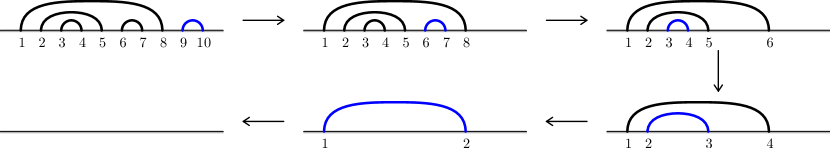
Figure 2.1: An allowable ordering of links in a link pattern $\alpha$ and the corresponding link removals.

Suppose the ordering $\{a_{1},b_{1}\},\ldots,\{a_{N},b_{N}\}$ of the links of $\alpha$ is allowable. Fix points $\xi_{j}\in(x_{a_{j}-1},x_{b_{j}+1})$ for all $j\in\{1,\ldots,N\}$, with the convention that $x_{0}=-\infty$ and $x_{2N+1}=+\infty$. It was proved in [FK15a, Lemma 10] that the following sequence of limits exists and is finite for any solution $F\in\mathcal{S}_{N}$:

$$\mathcal{L}_{\alpha}(F):=\lim_{x_{a_{N}},x_{b_{N}}\to\xi_{N}}\cdots\lim_{x_{a_{1}},x_{b_{1}}\to\xi_{1}}(x_{b_{N}}-x_{a_{N}})^{2h}\cdots(x_{b_{1}}-x_{a_{1}})^{2h}\,F(x_{1},\ldots,x_{2N}).$$ (2.10)

Furthermore, by [FK15a, Lemma 12], any other allowable ordering of the links of $\alpha$ gives the same limit (2.10). Therefore, for each $\alpha\in\mathrm{LP}_{N}$ with any choice of allowable ordering of links, (2.10) defines a linear functional

$$\mathcal{L}_{\alpha}\colon\mathcal{S}_{N}\to\mathbb{C}.$$

Finally, it was proved in [FK15c, Theorem 8] that, for any $\kappa\in(0,8)$, the collection $\{\mathcal{L}_{\alpha}\colon\alpha\in\mathrm{LP}_{N}\}$ is a basis for the dual space $\mathcal{S}_{N}^{*}$ of the $\mathrm{C}_{N}$-dimensional solution space $\mathcal{S}_{N}$.

2.4 Combinatorics and Binary Relation “$\;\stackrel{{\scriptstyle\scriptscriptstyle{()}}}{{\scriptstyle{\longleftarrow}}}\;$”

In this section, we introduce combinatorial objects closely related to the link patterns $\alpha\in\mathrm{LP}$, and present properties of them which are needed to complete the proof of Theorem 1.5 in Section 6. Results of this flavor appear in [KW11a, KW11b], and in [KKP17] for the context of pure partition functions. We follow the notations and conventions of the latter reference.

Dyck paths are walks on $\mathbb{Z}_{\geq 0}$ with steps of length one, starting and ending at zero. For $N\geq 1$, we denote the set of all Dyck paths of $2N$ steps by

$$\mathrm{DP}_{N}:=\big{\{}\alpha\colon\{0,1,\ldots,2N\}\rightarrow\mathbb{Z}_{\geq 0}\,\colon\,\alpha(0)=\alpha(2N)=0,\text{ and }|\alpha(k)-\alpha(k-1)|=1,\text{ for all }k\big{\}}.$$

To each link pattern $\alpha\in\mathrm{LP}_{N}$, we associate a Dyck path, also denoted by $\alpha\in\mathrm{DP}_{N}$, as follows. We write $\alpha$ as an ordered collection

$$\alpha=\{\{a_{1},b_{1}\},\ldots,\{a_{N},b_{N}\}\},\qquad\text{where }a_{1}<a_{2}<\cdots<a_{N}\text{ and }a_{j}<b_{j},\text{ for all }j\in\{1,\ldots,N\}.$$ (2.11)

Then, we set $\alpha(0)=0$ and, for all $k\in\{1,\ldots,2N\}$, we set

$$\alpha(k)=\begin{cases}\alpha(k-1)+1,&\text{if }k=a_{r}\text{ for some }r,\\ \alpha(k-1)-1,&\text{if }k=b_{s}\text{ for some }s.\end{cases}$$ (2.12)

Indeed, this defines a Dyck path $\alpha\in\mathrm{DP}_{N}$. Conversely, for any Dyck path $\alpha\colon\{0,1,\ldots,2N\}\rightarrow\mathbb{Z}_{\geq 0}$, we associate a link pattern $\alpha$ by associating to each up-step (i.e., step away from zero) an index $a_{r}$, for $r=1,2,\ldots,N$, and to each down-step (i.e., step towards zero) an index $b_{s}$, for $s=1,2,\ldots,N$, and setting $\alpha:=\{\{a_{1},b_{1}\},\ldots,\{a_{N},b_{N}\}\}$. These two mappings $\mathrm{LP}_{N}\to\mathrm{DP}_{N}$ and $\mathrm{DP}_{N}\to\mathrm{LP}_{N}$ define a bijection between the sets of link patterns and Dyck paths, illustrated in Figure 2.2. We thus identify the elements $\alpha$ of these two sets and use the indistinguishable notation $\alpha\in\mathrm{LP}_{N}$ and $\alpha\in\mathrm{DP}_{N}$ for both.

[capbesideposition=right,center,capbesidewidth=0.4]figure[]

Figure 2.2: Illustration of the bijection $\mathrm{LP}_{N}\leftrightarrow\mathrm{DP}_{N}$, identifying link patterns and Dyck paths for $\alpha=\{\{1,10\},\{2,5\},\{3,4\},\{6,7\},\{8,9\}\}$. Both the link pattern (top) and the Dyck path (bottom) are denoted by $\alpha$.

Figure 2.3: These two link patterns are comparable in the partial order $\preceq$, but incomparable in the binary relation $\stackrel{{\scriptstyle\scriptscriptstyle{()}}}{{\scriptstyle{\longleftarrow}}}$: the left link pattern is $\alpha=\{\{1,4\},\{2,3\},\{5,6\},\{7,8\}\}$ and the right link pattern is $\beta=\{\{1,8\},\{2,7\},\{3,6\},\{4,5\}\}$.

These sets have a natural partial order $\preceq$ measuring how nested their elements are: we define

$$\alpha\preceq\beta\qquad\text{ if and only if }\qquad\alpha(k)\leq\beta(k),\text{ for all }k\in\{0,1,\ldots,N\}.$$ (2.13)

For instance, the rainbow link pattern $\boldsymbol{\underline{\Cap}}_{N}$ is maximally nested — it is the largest element in this partial order. In fact, the partial order $\preceq$ is the transitive closure of a binary relation which was introduced by R. Kenyon and D. Wilson in [KW11a, KW11b] and K. Shigechi and P. Zinn-Justin in [SZ12]. We give a definition for this binary relation $\stackrel{{\scriptstyle\scriptscriptstyle{()}}}{{\scriptstyle{\longleftarrow}}}$ that we have found the most suitable to the purposes of the present article. We refer to [KKP17, Section 2] for a detailed survey of this binary relation and many equivalent definitions of it; see also Figure 2.3 for an example. We define $\stackrel{{\scriptstyle\scriptscriptstyle{()}}}{{\scriptstyle{\longleftarrow}}}$ as follows:

Definition 2.8.

[KKP17, Lemma 2.5] Let $\alpha=\{\{a_{1},b_{1}\},\ldots,\{a_{N},b_{N}\}\}\in\mathrm{LP}_{N}$ be ordered as in (2.11). Let $\beta\in\mathrm{LP}_{N}$. Then, $\alpha\stackrel{{\scriptstyle\scriptscriptstyle{()}}}{{\scriptstyle{\longleftarrow}}}\beta$ if and only if there exists a permutation $\sigma\in\mathfrak{S}_{N}$ such that

$$\beta=\{\{a_{1},b_{\sigma(1)}\},\ldots,\{a_{N},b_{\sigma(N)}\}\}.$$

For each $N\geq 1$, the incidence matrix $\mathcal{M}$ of this relation on the set $\mathrm{LP}_{N}\leftrightarrow\mathrm{DP}_{N}$ is the $\mathrm{C}_{N}\times\mathrm{C}_{N}$ matrix $\mathcal{M}=(\mathcal{M}_{\alpha,\beta})$ whose matrix elements are

$$\mathcal{M}_{\alpha,\beta}=\mathbb{1}\{\alpha\stackrel{{\scriptstyle\scriptscriptstyle{()}}}{{\scriptstyle{\longleftarrow}}}\beta\}=\begin{cases}1,&\text{ if }\alpha\stackrel{{\scriptstyle\scriptscriptstyle{()}}}{{\scriptstyle{\longleftarrow}}}\beta,\\ 0,&\text{ otherwise}.\end{cases}$$

In order to state and prove Theorem 1.5 in Section 6, we have to invert the matrix $\mathcal{M}$. For this purpose, we need some more combinatorics, related to skew-Young diagrams and their tilings. Let $\alpha\preceq\beta$. When the two Dyck paths $\alpha,\beta\in\mathrm{DP}_{N}$ are drawn on the same coordinate system, their difference forms a (rotated) skew Young diagram, denoted by $\alpha/\beta$, which can be thought of as a union of atomic squares — see Figure 2.4. We denote by $|\alpha/\beta|$ the number of atomic square tiles in the skew Young diagram $\alpha/\beta$.

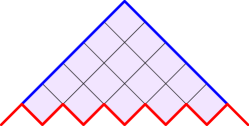
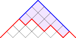
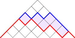
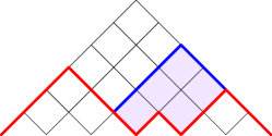
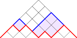
Figure 2.4: Skew Young diagrams $\alpha/\beta$. The smaller Dyck path $\alpha$ (resp. larger $\beta$) is red (resp. blue).

Consider then tilings of the skew Young diagram $\alpha/\beta$. The atomic square tiles form one possible tiling of $\alpha/\beta$, a rather trivial one. In this article, following the terminology of [KW11a, KW11b, KKP17], we consider tilings of $\alpha/\beta$ by Dyck tiles, called Dyck tilings. A Dyck tile is a non-empty union of atomic squares, where the midpoints of the squares form a shifted Dyck path, see Figure 2.5. Note that also an atomic square is a Dyck tile. A Dyck tiling $T$ of a skew Young diagram $\alpha/\beta$ is a collection of non-overlapping Dyck tiles whose union is $\bigcup T=\alpha/\beta$. Dyck tilings are also illustrated in Figure 2.5.

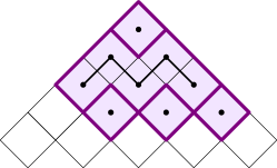
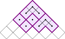
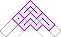
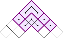
Figure 2.5: Examples of Dyck tilings, that is, tilings of a skew Young diagrams $\alpha/\beta$ by Dyck tiles.

The placement of a Dyck tile $t$ is given by the integer coordinates $(x_{t},h_{t})$ of the bottom left position of $t$, that is, the midpoint of the bottom left atomic square of $t$. If $(x^{\prime}_{t},h_{t})$ is the bottom right position of $t$, we call the closed interval $[x_{t},x^{\prime}_{t}]\subset\mathbb{R}$ the horizontal extent of $t$ — see Figure 2.6 for an illustration.

A Dyck tile $t_{1}$ is said to cover a Dyck tile $t_{2}$ if $t_{1}$ contains an atomic square which is an upward vertical translation of some atomic square of $t_{2}$. A Dyck tiling $T$ of $\alpha/\beta$ is said to be cover-inclusive if for any two distinct tiles of $T$, either the horizontal extents are disjoint, or the tile that covers the other has horizontal extent contained in the horizontal extent of the other. See Figures 2.5 and 2.6 for illustrations.

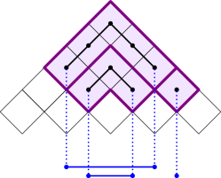
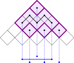
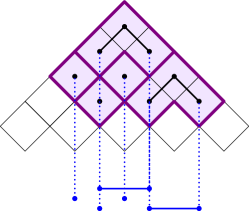
Figure 2.6: Examples of Dyck tilings with their horizontal extents illustrated. The two on the second row are cover-inclusive, but the three on the first row are not.

After these preparations, we are now ready to recall from [KW11b, KKP17] the following result, which enables us to write an explicit formula for the pure partition functions for $\kappa=4$ in Theorem 1.5.

Proposition 2.9.

The matrix $\mathcal{M}$ is invertible with inverse given by

$$\mathcal{M}^{-1}_{\alpha,\beta}=\begin{cases}(-1)^{|\alpha/\beta|}\#\mathcal{C}(\alpha/\beta),&\text{ if }\alpha\preceq\beta,\\ 0,&\text{ otherwise},\end{cases}$$

where $|\alpha/\beta|$ is the number of atomic square tiles in the skew Young diagram $\alpha/\beta$, and $\#\mathcal{C}(\alpha/\beta)$ denotes the number of cover-inclusive Dyck tilings of $\alpha/\beta$, with the convention that $\#\mathcal{C}(\alpha/\alpha)=1$.

Proof.

This follows immediately from [KKP17, Theorem 2.9] with tile weight $-1$. Originally, the proof appears in [KW11b, Theorems 1.5 and 1.6]. ∎

The entries $\mathcal{M}^{-1}_{\alpha,\beta}$ are always integers, and the diagonal entries are all equal to one: $\mathcal{M}^{-1}_{\alpha,\alpha}=1$ for all $\alpha$. Thus, the formula (1.9) in Theorem 1.5 is lower-triangular in the partial order $\succeq$. For instance, we have $\mathcal{Z}_{\boldsymbol{\underline{\Cap}}_{N}}=\mathcal{U}_{\boldsymbol{\underline{\Cap}}_{N}}$ for the rainbow link pattern. In Tables 1 and 2, we give examples of the matrix $\mathcal{M}$ and its inverse $\mathcal{M}^{-1}$.

$$\mathrm{LP}_{N}$$ with

1 0

1 1

            

with

1 0

-1 1

Table 1: The matrix elements of $\mathcal{M}$ (left) and $\mathcal{M}^{-1}$ (right) for $N=2$.

$$\mathrm{LP}_{N}$$ with

1 0 0 0 0

1 1 0 0 0

0 1 1 0 0

0 1 0 1 0

1 1 1 1 1

$$\mathrm{LP}_{N}$$ with

1 0 0 0 0

-1 1 0 0 0

1 -1 1 0 0

1 -1 0 1 0

-2 1 -1 -1 1

Table 2: The matrix elements of $\mathcal{M}$ (top) and $\mathcal{M}^{-1}$ (bottom) for $N=3$.

To finish this preliminary section, we introduce notation for certain combinatorial operations on Dyck paths and summarize results about them that are needed to complete the proof of Theorem 1.5 in Section 6. In the bijection $\mathrm{LP}_{N}\leftrightarrow\mathrm{DP}_{N}$ illustrated in Figure 2.2, a link between $j$ and $j+1$ in $\alpha\in\mathrm{LP}_{N}$ corresponds with an up-step followed by a down-step in the Dyck path $\alpha$, so $\{j,j+1\}\in\alpha$ is equivalent to $j$ being a local maximum of the Dyck path $\alpha\in\mathrm{DP}_{N}$. In this situation, we denote $\wedge^{j}\in\alpha$ and we say that $\alpha$ has an up-wedge at $j$. Down-wedges $\vee_{j}$ are defined analogously, and an unspecified local extremum is called a wedge $\lozenge_{j}$. Otherwise, we say that $\alpha$ has a slope at $j$, denoted by $\times_{j}\in\alpha$. When $\alpha$ has a down-wedge, $\vee_{j}\in\alpha$, we define the wedge-lifting operation $\alpha\mapsto\alpha\uparrow\lozenge_{j}$ by letting $\alpha\uparrow\lozenge_{j}$ be the Dyck path obtained by converting the down-wedge $\vee_{j}$ in $\alpha$ into an up-wedge $\wedge^{j}$.

We recall that, if a link pattern $\alpha\in\mathrm{LP}_{N}$ has a link $\{j,j+1\}\in\alpha$, then we denote by $\alpha/\{j,j+1\}\in\mathrm{LP}_{N-1}$ the link pattern obtained from $\alpha$ by removing the link $\{j,j+1\}$ and relabeling the remaining indices by $1,2,\ldots,2N-2$ (see Figure 1.2). In terms of the Dyck path, this operation is called an up-wedge removal and denoted by $\alpha\setminus\wedge^{j}\in\mathrm{DP}_{N-1}$. For Dyck paths, we can define a completely analogous down-wedge removal $\alpha\mapsto\alpha\setminus\vee_{j}$. Occasionally, it is not important to specify the type of wedge that is removed, so whenever $\alpha$ has either type of local extremum at $j$ (that is, $\lozenge_{j}\in\alpha$), we denote by $\alpha\setminus\lozenge_{j}\in\mathrm{DP}_{N-1}$ the two steps shorter Dyck path obtained by removing the two steps around $\lozenge_{j}$, see Figure 2.7.

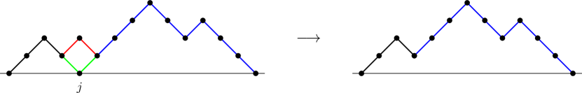
Figure 2.7: The removal of a wedge from a Dyck path. The left figure is the Dyck path $\alpha\in\mathrm{DP}_{N}$ and the right figure the shorter Dyck path $\alpha\setminus\lozenge_{j}\in\mathrm{DP}_{N-1}$, with $j=4$ and $N=7$.

Lemma 2.10.

The following statements hold for Dyck paths $\alpha,\beta\in\mathrm{DP}_{N}$.

• Suppose $\wedge^{j}\not\in\alpha$ and $\vee_{j}\in\beta$. Then, we have $\alpha\preceq\beta$ if and only if $\alpha\preceq\beta\uparrow\lozenge_{j}$.

• Suppose $\wedge^{j}\not\in\alpha$. Then the Dyck paths $\beta\in\mathrm{DP}_{N}$ such that $\beta\succeq\alpha$ and $\lozenge_{j}\in\beta$ come in pairs, one containing an up-wedge and the other a down-wedge at $j$:

  $$\{\beta\in\mathrm{DP}_{N}\colon\beta\succeq\alpha\}\;=\;\{\beta\colon\beta\succeq\alpha,\vee_{j}\in\beta\}\cup\{\beta\uparrow\lozenge_{j}\colon\beta\succeq\alpha,\vee_{j}\in\beta\}\cup\{\beta\colon\beta\succeq\alpha,\times_{j}\in\beta\}.$$

• Suppose $\wedge^{j}\in\beta$. Then, we have $\alpha\stackrel{{\scriptstyle\scriptscriptstyle{()}}}{{\scriptstyle{\longleftarrow}}}\beta$ if and only if $\lozenge_{j}\in\alpha$ and $\alpha\setminus\lozenge_{j}\stackrel{{\scriptstyle\scriptscriptstyle{()}}}{{\scriptstyle{\longleftarrow}}}\beta\setminus\wedge^{j}$.

• Suppose $\wedge^{j}\not\in\alpha$, $\vee_{j}\in\beta$, and $\alpha\preceq\beta$. Then we have $\mathcal{M}^{-1}_{\alpha,\beta}=-\mathcal{M}^{-1}_{\alpha,\beta\uparrow\lozenge_{j}}$.

Proof.

Parts (a) and (b) were proved, e.g., in [KKP17, Lemma 2.11] (see also the remark below that lemma). Part (c) was proved, e.g., in [KKP17, Lemma 2.12]. For completeness, we give a short proof for Part (d). First, [KKP17, Lemma 2.15] says that if $\wedge^{j}\not\in\alpha$, $\vee_{j}\in\beta$, and $\alpha\preceq\beta$, then we have $\#\mathcal{C}(\alpha/\beta)=\#\mathcal{C}\big{(}\alpha/(\beta\uparrow\lozenge_{j})\big{)}$. On the other hand, Proposition 2.9 shows that $\mathcal{M}^{-1}_{\alpha,\beta}=(-1)^{|\alpha/\beta|}\#\mathcal{C}(\alpha/\beta)$. The claim follows from this and the observation that the number of Dyck tiles in a cover-inclusive Dyck tiling of $\alpha/(\beta\uparrow\lozenge_{j})$ is one more than the number of Dyck tiles in a cover-inclusive Dyck tiling of $\alpha/\beta$, by [KKP17, proof of Lemma 2.15]. ∎

3 Global Multiple SLEs

Throughout this section, we fix the value of $\kappa\in(0,4]$ and we let $(\Omega;x_{1},\ldots,x_{2N})$ be a polygon. For each link pattern $\alpha=\{\{a_{1},b_{1}\},\ldots,\{a_{N},b_{N}\}\}\in\mathrm{LP}_{N}$, we construct an $N$-$\operatorname{SLE}_{\kappa}$ probability measure $\mathbb{Q}_{\alpha}^{\#}$ on the set $X_{0}^{\alpha}(\Omega;x_{1},\ldots,x_{2N})$ of pairwise disjoint, continuous simple curves $(\eta_{1},\ldots,\eta_{N})$ in $\Omega$ such that, for each $j\in\{1,\ldots,N\}$, the curve $\eta_{j}$ connects $x_{a_{j}}$ to $x_{b_{j}}$ according to $\alpha$ (see Proposition 3.3).

In [KL07] M. Kozdron and G. Lawler constructed such a probability measure in the special case when the curves form the rainbow connectivity, illustrated in Figure 3.1, encoded in the link pattern $\boldsymbol{\underline{\Cap}}_{N}=\{\{1,2N\},\{2,2N-1\},\ldots,\{N,N+1\}\}$ (see also [Dub06, Section 3.4]). The generalization of this construction to the case of any possible topological connectivity of the curves, encoded in a general link pattern $\alpha\in\mathrm{LP}_{N}$, was stated in Lawler’s works [Law09a, Law09b], but without proof.

In the present article, we give a combinatorial construction, which appears to agree with [Law09a, Section 2.7]. In contrast to the previous works, we formulate the result focusing on the conceptual definition of the global multiple $\operatorname{SLE}$s, instead of just defining them as weighted $\operatorname{SLE}$s. These $N$-$\operatorname{SLE}_{\kappa}$ measures have the defining property that, for each $j\in\{1,\ldots,N\}$, the conditional law of $\eta_{j}$ given $\{\eta_{1},\ldots,\eta_{j-1},\eta_{j+1},\ldots,\eta_{N}\}$ is the $\operatorname{SLE}_{\kappa}$ connecting $x_{a_{j}}$ and $x_{b_{j}}$ in the component $\hat{\Omega}_{j}$ of the domain $\Omega\setminus\{\eta_{1},\ldots,\eta_{j-1},\eta_{j+1},\ldots,\eta_{N}\}$ having $x_{a_{j}}$ and $x_{b_{j}}$ on its boundary. In subsequent work [BPW18], we prove that this property uniquely determines the global multiple $\operatorname{SLE}$ measures.

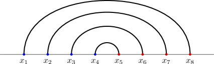
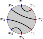
Figure 3.1: The rainbow link pattern with four links, denoted by $\boldsymbol{\underline{\Cap}}_{4}$.

3.1 Construction of Global Multiple SLEs

The general idea to construct global multiple $\operatorname{SLE}$s is that one defines the measure by its Radon-Nikodym derivative with respect to the product measure of independent chordal $\operatorname{SLE}$s. This Radon-Nikodym derivative can be written in terms of the Brownian loop measure. The same idea can also be used to construct multiple $\operatorname{SLE}$s in finitely connected domains, see [Law09a, Law09b, Law11].

Fix $\alpha=\{\{a_{1},b_{1}\},\ldots,\{a_{N},b_{N}\}\}\in\mathrm{LP}_{N}$. To construct the global $N$-$\operatorname{SLE}_{\kappa}$ associated to $\alpha$, we introduce a combinatorial expression of Brownian loop measures, denoted by $m_{\alpha}$. For each configuration $(\eta_{1},\ldots,\eta_{N})\in X_{0}^{\alpha}(\Omega;x_{1},\ldots,x_{2N})$, we note that $\Omega\setminus\{\eta_{1},\ldots,\eta_{N}\}$ has $N+1$ connected components (c.c). The boundary of each c.c. $\mathcal{C}$ contains some of the curves $\{\eta_{1},\ldots,\eta_{N}\}$. We denote by

$$\mathcal{B}(\mathcal{C}):=\{j\in\{1,\ldots,N\}\colon\eta_{j}\subset\partial\mathcal{C}\}$$

the set of indices $j$ specified by the curves $\eta_{j}\subset\partial\mathcal{C}$. If $\mathcal{B}(\mathcal{C})=\{j_{1},\ldots,j_{p}\}$, we define

$$m(\mathcal{C}):= \;\sum_{\begin{subarray}{c}i_{1},i_{2}\in\mathcal{B}(\mathcal{C}),\\ i_{1}\neq i_{2}\end{subarray}}\mu(\Omega;\eta_{i_{1}},\eta_{i_{2}})-\sum_{\begin{subarray}{c}i_{1},i_{2},i_{3}\in\mathcal{B}(\mathcal{C}),\\ i_{1}\neq i_{2}\neq i_{3}\neq i_{1}\end{subarray}}\mu(\Omega;\eta_{i_{1}},\eta_{i_{2}},\eta_{i_{3}})+\cdots+(-1)^{p}\mu(\Omega;\eta_{j_{1}},\ldots,\eta_{j_{p}}).$$

For $(\eta_{1},\ldots,\eta_{N})\in X_{0}^{\alpha}(\Omega;x_{1},\ldots,x_{2N})$, we define

$$m_{\alpha}(\Omega;\eta_{1},\ldots,\eta_{N}):=\sum_{\text{c.c. }\mathcal{C}\text{ of }\Omega\setminus\{\eta_{1},\ldots,\eta_{N}\}}m(\mathcal{C}).$$ (3.1)

If $\alpha$ is the rainbow pattern $\boldsymbol{\underline{\Cap}}_{N}$, then the quantity $m_{\alpha}$ has a simple expression:

$$m_{\boldsymbol{\underline{\Cap}}_{N}}(\Omega;\eta_{1},\ldots,\eta_{N})=\sum_{j=1}^{N-1}\mu(\Omega;\eta_{j},\eta_{j+1}),\qquad\text{for }\boldsymbol{\underline{\Cap}}_{N}=\{\{1,2N\},\{2,2N-1\},\ldots,\{N,N+1\}\}.$$

More generally, $m_{\alpha}$ is given by an inclusion-exclusion procedure that depends on $\alpha$. It has the following cascade property, which will be crucial in the sequel.

Lemma 3.1.

Let $\alpha\in\mathrm{LP}_{N}$ and $j\in\{1,\ldots,N\}$, and denote $\hat{\alpha}=\alpha/\{a_{j},b_{j}\}\in\mathrm{LP}_{N-1}$. Then we have

$$m_{\alpha}(\Omega;\eta_{1},\ldots,\eta_{N})=m_{\hat{\alpha}}(\Omega;\eta_{1},\ldots,\eta_{j-1},\eta_{j+1},\ldots,\eta_{N})+\mu(\Omega;\eta_{j},\Omega\setminus\hat{\Omega}_{j}),$$

where $\hat{\Omega}_{j}$ is the connected component of $\Omega\setminus\{\eta_{1},\ldots,\eta_{j-1},\eta_{j+1},\ldots,\eta_{N}\}$ having $x_{a_{j}}$ and $x_{b_{j}}$ on its boundary.

Proof.

As illustrated in Figure 3.2, the domain $\Omega\setminus\{\eta_{1},\ldots,\eta_{N}\}$ has $N+1$ connected components, two of which have the curve $\eta_{j}$ on their boundary. We denote them by $\mathcal{C}^{L}_{j}$ and $\mathcal{C}^{R}_{j}$. We split the summation in $m_{\alpha}$ into two parts, depending on whether or not $\eta_{j}$ is a part of the boundary of the c.c. $\mathcal{C}$:

$$m_{\alpha}(\Omega;\eta_{1},\ldots,\eta_{N})=S_{1}+S_{2},\qquad\text{where }\quad S_{1}=m(\mathcal{C}^{L}_{j})+m(\mathcal{C}^{R}_{j})\quad\text{ and }\quad S_{2}=\sum_{\mathcal{C}\;:\;j\notin\mathcal{B}(\mathcal{C})}m(\mathcal{C}).$$

The quantity $S_{1}$ is a sum of terms of the form $\mu(\Omega;\eta_{i_{1}},\ldots,\eta_{i_{k}})$. We split the terms in $S_{1}=S_{1,1}+S_{1,2}$ into two parts: $S_{1,1}$ is the sum of the terms in $S_{1}$ including $\eta_{j}$ and $S_{1,2}$ is the sum of the terms in $S_{1}$ excluding $\eta_{j}$. Now we have $m_{\alpha}(\Omega;\eta_{1},\ldots,\eta_{N})=S_{1,1}+S_{1,2}+S_{2}$.

On the other hand, by definition (3.1), the quantity $m_{\hat{\alpha}}$ can be written in the form

$$m_{\hat{\alpha}}(\Omega;\eta_{1},\ldots,\eta_{j-1},\eta_{j+1},\ldots,\eta_{N})=S_{2}+S_{1,2}+S_{3},$$

where $S_{3}$ contains the contribution of terms of type $\mu(\Omega;\eta_{i_{1}},\ldots,\eta_{i_{k}})$ for curves $\eta_{i_{1}},\ldots,\eta_{i_{k}}$ such that $i_{1},\ldots,i_{k}\in\mathcal{B}(\hat{\Omega}_{j})$ and at least two of these curves belong to different $\partial\mathcal{C}^{L}_{j}$ and $\partial\mathcal{C}^{R}_{j}$. For such curves, any Brownian loop intersecting all of them must also intersect $\eta_{j}$. Thus, we have $\mu(\Omega;\eta_{j},\Omega\setminus\hat{\Omega}_{j})=S_{1,1}-S_{3}$. The asserted identity follows:

$$m_{\alpha}(\Omega;\eta_{1},\ldots,\eta_{N}) =S_{1,1}-S_{3}+S_{3}+S_{1,2}+S_{2}$$

$$=\mu(\Omega;\eta_{j},\Omega\setminus\hat{\Omega}_{j})+m_{\hat{\alpha}}(\Omega;\eta_{1},\ldots,\eta_{j-1},\eta_{j+1},\ldots,\eta_{N}).$$

∎

[capbesideposition=right,center,capbesidewidth=0.5]figure[]

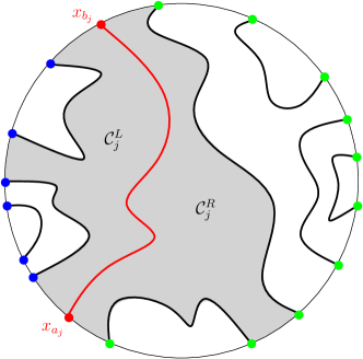
Figure 3.2: Illustration of notations used throughout.
The red curve is $\eta_{j}$. The domain $\Omega\setminus\{\eta_{1},\ldots,\eta_{N}\}$ has $N+1$ connected components. Two of them have $\eta_{j}$ on their boundary, denoted by $\mathcal{C}^{L}_{j}$ and $\mathcal{C}^{R}_{j}$. The grey domain is $\hat{\Omega}_{j}$, that is, the connected component of $\Omega\setminus\{\eta_{1},\ldots,\eta_{j-1},\eta_{j+1},\ldots,\eta_{N}\}$ having the endpoints $x_{a_{j}},x_{b_{j}}\in\partial\hat{\Omega}_{j}$ of the curve $\eta_{j}$ on its boundary.
On the other hand, in Proposition 3.5 we denote by $\eta=\eta_{j}$ and $D_{\eta}^{L}$ and $D_{\eta}^{R}$ the two connected components of $\Omega\setminus\eta$ on the left and right of the curve, respectively. The sub-link patterns of $\alpha$ associated to these two components are denoted by $\alpha^{L}$ and $\alpha^{R}$, and illustrated in blue and green in the figure.

Next, we record a boundary perturbation property for the quantity $m_{\alpha}$, also needed later.

Lemma 3.2.

Suppose $K$ is a relatively compact subset of $\Omega$ such that $\Omega\setminus K$ is simply connected, and assume that the distance between $K$ and $\{\eta_{1},\ldots,\eta_{N}\}$ is strictly positive. Then we have

$$m_{\alpha}(\Omega;\eta_{1},\ldots,\eta_{N})=m_{\alpha}(\Omega\setminus K;\eta_{1},\ldots,\eta_{N})+\sum_{j=1}^{N}\mu(\Omega;K,\eta_{j})-\mu\big{(}\Omega;K,\bigcup_{j=1}^{N}\eta_{j}\big{)}.$$ (3.2)

Proof.

We prove the asserted identity by induction on $N\geq 1$. For $N=1$, we have $m_{\vbox{\hbox{\includegraphics[scale={0.2}]{figures/link-0.pdf}}}}(\Omega;\eta)=0$, so the claim is clear. Assume that (3.2) holds for all link patterns in $\mathrm{LP}_{N-1}$, denote $\hat{\alpha}=\alpha/\{x_{a_{1}},x_{b_{1}}\}\in\mathrm{LP}_{N-1}$, and let $\eta_{1}$ be the curve from $x_{a_{1}}$ to $x_{b_{1}}$. Finally, let $\hat{\Omega}_{1}$ be the connected component of $\Omega\setminus\{\eta_{2},\ldots,\eta_{N}\}$ having the endpoints of $\eta_{1}$ on its boundary (as in Figure 3.2). Using Lemma 3.1 and the obvious fact that $\mu(\Omega;\eta_{1},\Omega\setminus\hat{\Omega}_{1})=\mu(\Omega\setminus K;\eta_{1},\Omega\setminus\hat{\Omega}_{1})+\mu(\Omega;K,\eta_{1},\Omega\setminus\hat{\Omega}_{1})$, we can write $m_{\alpha}$ in the form

$$m_{\alpha}(\Omega;\eta_{1},\ldots,\eta_{N})= \;m_{\hat{\alpha}}(\Omega;\eta_{2},\ldots,\eta_{N})+\mu(\Omega;\eta_{1},\Omega\setminus\hat{\Omega}_{1})$$

$$= \;m_{\hat{\alpha}}(\Omega;\eta_{2},\ldots,\eta_{N})+\mu(\Omega\setminus K;\eta_{1},\Omega\setminus\hat{\Omega}_{1})+\mu(\Omega;K,\eta_{1},\Omega\setminus\hat{\Omega}_{1}).$$

By the induction hypothesis, for $\hat{\alpha}\in\mathrm{LP}_{N-1}$, we have

$$m_{\hat{\alpha}}(\Omega;\eta_{2},\ldots,\eta_{N})=m_{\hat{\alpha}}(\Omega\setminus K;\eta_{2},\ldots,\eta_{N})+\sum_{j=2}^{N}\mu(\Omega;K,\eta_{j})-\mu\big{(}\Omega;K,\bigcup_{j=2}^{N}\eta_{j}\big{)}.$$

Combining these two relations with Lemma 3.1, we obtain

$$m_{\alpha}(\Omega;\eta_{1},\ldots,\eta_{N})=\; m_{\alpha}(\Omega\setminus K;\eta_{1},\ldots,\eta_{N})+\sum_{j=2}^{N}\mu(\Omega;K,\eta_{j})-\mu\big{(}\Omega;K,\bigcup_{j=2}^{N}\eta_{j}\big{)}+\mu(\Omega;K,\eta_{1},\Omega\setminus\hat{\Omega}_{1}).$$

Note now that $\mu(\Omega;K,\eta_{1},\Omega\setminus\hat{\Omega}_{1})=\mu\big{(}\Omega;K,\eta_{1},\bigcup_{j=2}^{N}\eta_{j}\big{)}$, so

$$\mu\big{(}\Omega;K,\bigcup_{j=1}^{N}\eta_{j}\big{)}= \;\mu(\Omega;K,\eta_{1})+\mu\big{(}\Omega;K,\bigcup_{j=2}^{N}\eta_{j}\big{)}-\mu\big{(}\Omega;K,\eta_{1},\bigcup_{j=2}^{N}\eta_{j}\big{)}$$

$$= \;\mu(\Omega;K,\eta_{1})+\mu\big{(}\Omega;K,\bigcup_{j=2}^{N}\eta_{j}\big{)}-\mu(\Omega;K,\eta_{1},\Omega\setminus\hat{\Omega}_{1}).$$

Combining the above two equations, we get the asserted identity (3.2):

$$m_{\alpha}(\Omega;\eta_{1},\ldots,\eta_{N})=m_{\alpha}(\Omega\setminus K;\eta_{1},\ldots,\eta_{N})+\sum_{j=2}^{N}\mu(\Omega;K,\eta_{j})-\mu(\Omega;K,\bigcup_{j=1}^{N}\eta_{j})+\mu(\Omega;K,\eta_{1}).$$

∎

Now, we are ready to construct the probability measure of Theorem 1.3.

Proposition 3.3.

Let $\kappa\in(0,4]$ and let $(\Omega;x_{1},\ldots,x_{2N})$ be a polygon. For any $\alpha\in\mathrm{LP}_{N}$, there exists a global $N$-$\operatorname{SLE}_{\kappa}$ associated to $\alpha$.

Proof.

For $\alpha=\{\{a_{1},b_{1}\},\ldots,\{a_{N},b_{N}\}\}\in\mathrm{LP}_{N}$, let $\mathbb{P}_{\alpha}$ denote the product measure

$$\mathbb{P}_{\alpha}:=\bigotimes_{j=1}^{N}\mathbb{P}(\Omega;x_{a_{j}},x_{b_{j}})$$

of $N$ independent chordal $\operatorname{SLE}_{\kappa}$ curves connecting the boundary points $x_{a_{j}}$ and $x_{b_{j}}$ for $j\in\{1,2,\ldots,N\}$ according to the connectivity $\alpha$. Denote by $\mathbb{E}_{\alpha}$ the expectation with respect to $\mathbb{P}_{\alpha}$. Define $\mathbb{Q}_{\alpha}$ to be the measure which is absolutely continuous with respect to $\mathbb{P}_{\alpha}$ with Radon-Nikodym derivative

$$\frac{\mathrm{d}\mathbb{Q}_{\alpha}}{\mathrm{d}\mathbb{P}_{\alpha}}(\eta_{1},\ldots,\eta_{N})=R_{\alpha}(\Omega;\eta_{1},\ldots,\eta_{N}):=\mathbb{1}_{\{\eta_{j}\cap\eta_{k}=\emptyset\;\forall\;j\neq k\}}\exp(cm_{\alpha}(\Omega;\eta_{1},\ldots,\eta_{N})).$$ (3.3)

First, we prove that the total mass $|\mathbb{Q}_{\alpha}|=\mathbb{E}_{\alpha}[R_{\alpha}(\Omega;\eta_{1},\ldots,\eta_{N})]$ of $\mathbb{Q}_{\alpha}$ is positive and finite. Positivity is clear from the definition (3.3). We prove the finiteness by induction on $N\geq 1$, using the cascade property of Lemma 3.1. The initial case $N=1$ is obvious: $R_{\vbox{\hbox{\includegraphics[scale={0.2}]{figures/link-0.pdf}}}}=1$. Let $N\geq 2$ and assume that $|\mathbb{Q}_{\hat{\alpha}}|$ is finite for all $\hat{\alpha}\in\mathrm{LP}_{N-1}$. Using Lemma 3.1, we write the Radon-Nikodym derivative (3.3) in the form

$$R_{\alpha}(\Omega;\eta_{1},\ldots,\eta_{N})=R_{\hat{\alpha}}(\Omega;\eta_{1},\ldots,\eta_{j-1},\eta_{j+1},\ldots,\eta_{N})\times\mathbb{1}_{\{\eta_{j}\subset\hat{\Omega}_{j}\}}\exp(c\mu(\Omega;\eta_{j},\Omega\setminus\hat{\Omega}_{j})),$$ (3.4)

for a fixed $j\in\{1,\ldots,N\}$, where $\hat{\alpha}=\alpha/\{a_{j},b_{j}\}$. Thus, we have

$$\mathbb{E}_{\alpha}[R_{\alpha}(\Omega;\eta_{1},\ldots,\eta_{N})]=\; \mathbb{E}_{\alpha}\big{[}\mathbb{E}_{\alpha}\left[R_{\alpha}(\Omega;\eta_{1},\ldots,\eta_{N})\,|\,\eta_{1},\ldots,\eta_{j-1},\eta_{j+1},\ldots,\eta_{N}\right]\big{]}$$

$$=\; \mathbb{E}_{\hat{\alpha}}\bigg{[}R_{\hat{\alpha}}(\Omega;\eta_{1},\ldots,\eta_{j-1},\eta_{j+1},\ldots,\eta_{N})\left(\frac{H_{\hat{\Omega}_{j}}(x_{a_{j}},x_{b_{j}})}{H_{\Omega}(x_{a_{j}},x_{b_{j}})}\right)^{h}\bigg{]}$$ [by Lemma 2.2]

$$\leq\; \mathbb{E}_{\hat{\alpha}}\left[R_{\hat{\alpha}}(\Omega;\eta_{1},\ldots,\eta_{j-1},\eta_{j+1},\ldots,\eta_{N})\right]$$ [by (2.3)]

$$\leq\; 1.$$ [by ind. hypothesis]

Noting that the Radon-Nikodym derivative (3.3) also depends on the fixed boundary points $x_{1},\ldots,x_{2N}$, we define the function $f_{\alpha}$ of $2N$ variables $x_{1},\ldots,x_{2N}\in\partial\Omega$ by

$$f_{\alpha}(\Omega;x_{1},\ldots,x_{2N}):=\mathbb{E}_{\alpha}[R_{\alpha}(\Omega;\eta_{1},\ldots,\eta_{N})]=|\mathbb{Q}_{\alpha}|.$$ (3.5)

Note that $f_{\alpha}$ is conformally invariant. From the above analysis, we see that it is also bounded:

$$0<f_{\alpha}\leq 1.$$ (3.6)

Second, we show that, for each $j\in\{1,\ldots,N\}$, under the probability measure $\mathbb{Q}_{\alpha}^{\#}:=\mathbb{Q}_{\alpha}/|\mathbb{Q}_{\alpha}|$, the conditional law of $\eta_{j}$ given $\{\eta_{1},\ldots,\eta_{j-1},\eta_{j+1},\ldots,\eta_{N}\}$ is the $\operatorname{SLE}_{\kappa}$ connecting $x_{a_{j}}$ and $x_{b_{j}}$ in the domain $\hat{\Omega}_{j}$. By the cascade property (3.4), given $\{\eta_{1},\ldots,\eta_{j-1},\eta_{j+1},\ldots,\eta_{N}\}$, the conditional law of $\eta_{j}$ is the same as $\mathbb{P}(\Omega;x_{a_{j}},x_{b_{j}})$ weighted by $\mathbb{1}_{\{\eta_{j}\subset\hat{\Omega}_{j}\}}\exp(c\mu(\Omega;\eta_{j},\Omega\setminus\hat{\Omega}_{j}))$. Now, by Lemma 2.2, this is the same as the law of the $\operatorname{SLE}_{\kappa}$ in $\hat{\Omega}_{j}$ connecting $x_{a_{j}}$ and $x_{b_{j}}$. This completes the proof. ∎

3.2 Properties of Global Multiple SLEs

Next, we prove useful properties of global multiple $\operatorname{SLE}$s: first, we establish a boundary perturbation property, and then a cascade property describing the marginal law of one curve in a global multiple $\operatorname{SLE}$.

To begin, we set $\mathcal{B}_{\emptyset}:=1$ and $\mathcal{Z}_{\emptyset}:=1$, and define, for all integers $N\geq 1$ and link patterns $\alpha\in\mathrm{LP}_{N}$, the bound function $\mathcal{B}_{\alpha}$ and the pure partition function $\mathcal{Z}_{\alpha}$ as

$$\begin{split}\mathcal{B}_{\alpha}\colon\mathfrak{X}_{2N}\to\mathbb{R}_{>0},\qquad\qquad&\mathcal{B}_{\alpha}(x_{1},\ldots,x_{2N}):=\prod_{\{a,b\}\in\alpha}|x_{b}-x_{a}|^{-1},\\ \mathcal{Z}_{\alpha}\colon\mathfrak{X}_{2N}\to\mathbb{R}_{>0},\qquad\qquad&\mathcal{Z}_{\alpha}(x_{1},\ldots,x_{2N}):=f_{\alpha}(\mathbb{H};x_{1},\ldots,x_{2N})\,\mathcal{B}_{\alpha}(x_{1},\ldots,x_{2N})^{2h},\end{split}$$ (3.7)

where $f_{\alpha}=|\mathbb{Q}_{\alpha}|$ is the function defined in (3.5).

If the points $x_{1},\ldots,x_{2N}$ of the polygon $(\Omega;x_{1},\ldots,x_{2N})$ lie on sufficiently regular boundary segments (e.g., $C^{1+\epsilon}$ for some $\epsilon>0$), we call $(\Omega;x_{1},\ldots,x_{2N})$ a nice polygon. For a nice polygon $(\Omega;x_{1},\ldots,x_{2N})$, we define

$$\begin{split}&\mathcal{B}_{\alpha}(\Omega;x_{1},\ldots,x_{2N}):=\prod_{\{a,b\}\in\alpha}H_{\Omega}(x_{a},x_{b})^{1/2},\\ &\mathcal{Z}_{\alpha}(\Omega;x_{1},\ldots,x_{2N}):=f_{\alpha}(\Omega;x_{1},\ldots,x_{2N})\,\mathcal{B}_{\alpha}(\Omega;x_{1},\ldots,x_{2N})^{2h}.\end{split}$$ (3.8)

This definition agrees with (1.5), by the conformal covariance property of the boundary Poisson kernel $H_{\Omega}$ and the conformal invariance property of $f_{\alpha}$. We also note that the bounds (3.6) show that

$$\mathcal{Z}_{\alpha}(\Omega;x_{1},\ldots,x_{2N})\leq\mathcal{B}_{\alpha}(\Omega;x_{1},\ldots,x_{2N})^{2h}.$$ (3.9)

3.2.1 Boundary Perturbation Property

Multiple $\operatorname{SLE}$s have a boundary perturbation property analogous to Lemma 2.2. To state it, we use the specific notation $\mathbb{Q}_{\alpha}^{\#}(\Omega;x_{1},\ldots,x_{2N})$ for the global $N$-$\operatorname{SLE}_{\kappa}$ probability measure associated to the link pattern $\alpha=\{\{a_{1},b_{1}\},\ldots,\{a_{N},b_{N}\}\}\in\mathrm{LP}_{N}$ in the polygon $(\Omega;x_{1},\ldots,x_{2N})$.

Proposition 3.4.

Let $\kappa\in(0,4]$. Let $(\Omega;x_{1},\ldots,x_{2N})$ be a polygon and $U\subset\Omega$ a sub-polygon. Then, the probability measure $\mathbb{Q}_{\alpha}^{\#}(U;x_{1},\ldots,x_{2N})$ is absolutely continuous with respect to $\mathbb{Q}_{\alpha}^{\#}(\Omega;x_{1},\ldots,x_{2N})$, with Radon-Nikodym derivative

$$\frac{\mathrm{d}\mathbb{Q}_{\alpha}^{\#}(U;x_{1},\ldots,x_{2N})}{\mathrm{d}\mathbb{Q}_{\alpha}^{\#}(\Omega;x_{1},\ldots,x_{2N})}(\eta_{1},\ldots,\eta_{N})\,=\,\frac{\mathcal{Z}_{\alpha}(\Omega;x_{1},\ldots,x_{2N})}{\mathcal{Z}_{\alpha}(U;x_{1},\ldots,x_{2N})}\;\mathbb{1}_{\{\eta_{j}\subset U\;\forall\;j\}}\exp\bigg{(}c\mu\Big{(}\Omega;\Omega\setminus U,\bigcup_{j=1}^{N}\eta_{j}\Big{)}\bigg{)}.$$

Moreover, if $\kappa\leq 8/3$ and $(\Omega;x_{1},\ldots,x_{2N})$ is a nice polygon, then we have

$$\mathcal{Z}_{\alpha}(\Omega;x_{1},\ldots,x_{2N})\geq\mathcal{Z}_{\alpha}(U;x_{1},\ldots,x_{2N}).$$ (3.10)

Proof.

From the formula (3.3) and Lemma 3.2, we see that

$$\mathbb{1}_{\{\eta_{j}\subset U\;\forall\;j\}}\;\mathrm{d}\mathbb{Q}_{\alpha}(\Omega;x_{1},\ldots,x_{2N})$$

$$= \;\mathbb{1}_{\{\eta_{j}\subset U\;\forall\;j\}}\mathbb{1}_{\{\eta_{j}\cap\eta_{k}=\emptyset\;\forall\;j\neq k\}}\;\exp(cm_{\alpha}(\Omega;\eta_{1},\ldots,\eta_{N}))\;\mathrm{d}\mathbb{P}_{\alpha}$$

$$= \;\mathbb{1}_{\{\eta_{j}\subset U\;\forall\;j\}}\mathbb{1}_{\{\eta_{j}\cap\eta_{k}=\emptyset\;\forall\;j\neq k\}}\;\exp(cm_{\alpha}(U;\eta_{1},\ldots,\eta_{N}))\;\exp\bigg{(}-c\mu\Big{(}\Omega;\Omega\setminus U,\bigcup_{j=1}^{N}\eta_{j}\Big{)}\bigg{)}$$

$$\times\prod_{j=1}^{N}\exp\left(c\mu(\Omega;\Omega\setminus U,\eta_{j})\right)\;\mathrm{d}\mathbb{P}(\Omega;x_{a_{j}},x_{b_{j}})$$

By Lemma 2.2, we have

$$\mathbb{1}_{\{\eta_{j}\subset U\;\forall\;j\}}\;\mathrm{d}\mathbb{Q}_{\alpha}(\Omega;x_{1},\ldots,x_{2N})$$

$$= \;\mathbb{1}_{\{\eta_{j}\cap\eta_{k}=\emptyset\;\forall\;j\neq k\}}\;\exp(cm_{\alpha}(U;\eta_{1},\ldots,\eta_{N}))\;\exp\bigg{(}-c\mu\Big{(}\Omega;\Omega\setminus U,\bigcup_{j=1}^{N}\eta_{j}\Big{)}\bigg{)}$$

$$\times\prod_{j=1}^{N}\left(\frac{H_{U}(x_{a_{j}},x_{b_{j}})}{H_{\Omega}(x_{a_{j}},x_{b_{j}})}\right)^{h}\;\mathrm{d}\mathbb{P}(U;x_{a_{j}},x_{b_{j}})$$

$$= \;\exp\bigg{(}-c\mu\Big{(}\Omega;\Omega\setminus U,\bigcup_{j=1}^{N}\eta_{j}\Big{)}\bigg{)}\prod_{j=1}^{N}\left(\frac{H_{U}(x_{a_{j}},x_{b_{j}})}{H_{\Omega}(x_{a_{j}},x_{b_{j}})}\right)^{h}\;\mathrm{d}\mathbb{Q}_{\alpha}(U;x_{1},\ldots,x_{2N}).$$

Combining this with the definition (3.8), we obtain the asserted Radon-Nikodym derivative. The monotonicity property (3.10) follows from the fact that when $\kappa\leq 8/3$, we have $c\leq 0$ and thus,

$$1\geq\mathbb{P}[\eta_{j}\subset U\;\text{ for all }j]\geq\frac{\mathcal{Z}_{\alpha}(U;x_{1},\ldots,x_{2N})}{\mathcal{Z}_{\alpha}(\Omega;x_{1},\ldots,x_{2N})}.$$

This concludes the proof. ∎

3.2.2 Marginal Law

Next we prove a cascade property for the measure $\mathbb{Q}_{\alpha}^{\#}$. Given any link $\{a,b\}\in\alpha$, let $\eta$ be the curve connecting $x_{a}$ and $x_{b}$ in the global $N$-$\operatorname{SLE}_{\kappa}$ with law $\mathbb{Q}_{\alpha}^{\#}$, as in Theorem 1.3. Assume that $a<b$ for notational simplicity. Then, the link $\{a,b\}$ divides the link pattern $\alpha$ into two sub-link patterns, connecting respectively the points $\{a+1,\ldots,b-1\}$ and $\{b+1,\ldots,a-1\}$. After relabeling of the indices, we denote these two link patterns by $\alpha^{R}$ and $\alpha^{L}$. Also, the domain $\Omega\setminus\eta$ has two connected components, which we denote by $D_{\eta}^{L}$ and $D_{\eta}^{R}$. The notations are illustrated in Figure 3.2.

Proposition 3.5.

The marginal law of $\eta$ under $\mathbb{Q}_{\alpha}^{\#}$ is absolutely continuous with respect to the law $\mathbb{P}(\Omega;x_{a},x_{b})$ of the $\operatorname{SLE}_{\kappa}$ connecting $x_{a}$ and $x_{b}$, with Radon-Nikodym derivative

$$\frac{H_{\Omega}(x_{a},x_{b})^{h}}{\mathcal{Z}_{\alpha}(\Omega;x_{1},\ldots,x_{2N})}\;\mathcal{Z}_{\alpha^{L}}(D_{\eta}^{L};x_{b+1},x_{b+2},\ldots,x_{a-1})\;\mathcal{Z}_{\alpha^{R}}(D_{\eta}^{R};x_{a+1},x_{a+2},\ldots,x_{b-1}).$$

Proof.

Note that the points $x_{b+1},\ldots,x_{a-1}$ (resp. $x_{a+1},\ldots,x_{b-1}$) lie along the boundary of $D_{\eta}^{L}$ (resp. $D_{\eta}^{R}$) in counterclockwise order. Denote by $(\eta_{1},\ldots,\eta_{N})\in X_{0}^{\alpha}(\Omega;x_{1},\ldots,x_{2N})$ the global $N$-$\operatorname{SLE}_{\kappa}$ with law $\mathbb{Q}_{\alpha}^{\#}$. Amongst the curves other than $\eta$, we denote by $\eta_{1}^{L},\ldots,\eta_{l}^{L}$ the ones contained in $D_{\eta}^{L}$ and by $\eta^{R}_{1},\ldots,\eta^{R}_{r}$ the ones contained in $D_{\eta}^{R}$ (so $l+r=N-1$).

First, we prove by induction on $N\geq 1$ that

$$m_{\alpha}(\Omega;\eta_{1},\ldots,\eta_{N})=m_{\alpha^{L}}(D_{\eta}^{L};\eta_{1}^{L},\ldots,\eta_{l}^{L})+m_{\alpha^{R}}(D_{\eta}^{R};\eta_{1}^{R},\ldots,\eta^{R}_{r})+\sum_{\eta^{\prime}\neq\eta}\mu(\Omega;\eta,\eta^{\prime}).$$ (3.11)

Equation (3.11) trivially holds for $N=1$, since $m_{\emptyset}=0=m_{\vbox{\hbox{\includegraphics[scale={0.2}]{figures/link-0.pdf}}}}$. By symmetry, we may assume that $\{a,b\}\neq\{2N-1,2N\}\in\alpha\,\cap\,\alpha^{L}$. Then, we let $\eta_{1}=\eta_{1}^{L}\subset D_{\eta}^{L}$ be the curve connecting $x_{2N-1}$ and $x_{2N}$, denote $\hat{\alpha}=\alpha/\{2N-1,2N\}$, and define $\hat{\alpha}^{L}$ and $\hat{\alpha}^{R}$ similarly as above — so $\alpha^{L}=\hat{\alpha}^{L}\cup\{\{2N-1,2N\}\}$ and $\hat{\alpha}^{R}=\alpha^{R}$. Applying Lemma 3.1 and the induction hypothesis, we get

$$m_{\alpha}(\Omega;\eta_{1},\ldots,\eta_{N}) =m_{\hat{\alpha}}(\Omega;\eta_{2},\ldots,\eta_{N})+\mu(\Omega;\eta_{1},\Omega\setminus\hat{\Omega}_{1})$$

$$=m_{\hat{\alpha}^{L}}(D_{\eta}^{L};\eta^{L}_{2},\ldots,\eta^{L}_{l})+m_{\alpha^{R}}(D_{\eta}^{R};\eta_{1}^{R},\ldots,\eta_{r}^{R})+\sum_{\eta^{\prime}\neq\eta,\eta_{1}}\mu(\Omega;\eta,\eta^{\prime})+\mu(\Omega;\eta_{1},\Omega\setminus\hat{\Omega}_{1}).$$

Combining this with the decomposition $\mu(\Omega;\eta_{1},\Omega\setminus\hat{\Omega}_{1})=\mu(D_{\eta}^{L};\eta_{1},D_{\eta}^{L}\setminus\hat{\Omega}_{1})+\mu(\Omega;\eta_{1},\eta)$, we obtain

$$m_{\alpha}(\Omega;\eta_{1},\ldots,\eta_{N}) =m_{\hat{\alpha}^{L}}(D_{\eta}^{L};\eta^{L}_{2},\ldots,\eta^{L}_{l})+\mu(D_{\eta}^{L};\eta_{1},D_{\eta}^{L}\setminus\hat{\Omega}_{1})+m_{\alpha^{R}}(D_{\eta}^{R};\eta_{1}^{R},\ldots,\eta_{r}^{R})+\sum_{\eta^{\prime}\neq\eta}\mu(\Omega;\eta,\eta^{\prime})$$

$$=m_{\alpha^{L}}(D_{\eta}^{L};\eta_{1}^{L},\ldots,\eta^{L}_{l})+m_{\alpha^{R}}(D_{\eta}^{R};\eta_{1}^{R},\ldots,\eta_{r}^{R})+\sum_{\eta^{\prime}\neq\eta}\mu(\Omega;\eta,\eta^{\prime}),$$

by Lemma 3.1. This completes the proof of the identity (3.11).

Next, we prove the proposition. From (3.3), we see that

$$\mathrm{d}\mathbb{Q}_{\alpha}= \;\mathbb{1}_{\{\eta_{i}\cap\eta_{k}=\emptyset\;\forall\;i\neq k\}}\;\exp(cm_{\alpha}(\Omega;\eta_{1},\ldots,\eta_{N}))\prod_{\{c,d\}\in\alpha}\;\mathrm{d}\mathbb{P}(\Omega;x_{c},x_{d})$$

$$= \;\mathbb{1}_{\{\eta_{i}\cap\eta_{k}=\emptyset\;\forall\;i\neq k\}}\;\exp\left(cm_{\alpha^{L}}(D_{\eta}^{L};\eta_{1}^{L},\ldots,\eta^{L}_{l})\right)\;\exp\left(cm_{\alpha^{R}}(D_{\eta}^{R};\eta^{R}_{1},\ldots,\eta_{r}^{R})\right)$$

$$\times\prod_{\eta^{\prime}\neq\eta}\exp(c\mu(\Omega;\eta,\eta^{\prime}))\prod_{\begin{subarray}{c}\{c,d\}\in\alpha,\\ \{c,d\}\neq\{a,b\}\end{subarray}}\;\mathrm{d}\mathbb{P}(\Omega;x_{c},x_{d})\times\mathrm{d}\mathbb{P}(\Omega;x_{a},x_{b})$$ [by (3.11)]

$$= \;\mathbb{1}_{\{\eta_{i}\cap\eta_{k}=\emptyset\;\forall\;i\neq k\}}\;\mathrm{d}\mathbb{P}(\Omega;x_{a},x_{b})$$ [by Lemma 2.2]

$$\times\exp\left(cm_{\alpha^{L}}(D_{\eta}^{L};\eta_{1}^{L},\ldots,\eta^{L}_{l})\right)\;\prod_{\{c,d\}\in\alpha^{L}}\left(\frac{H_{D_{\eta}^{L}}(x_{c},x_{d})}{H_{\Omega}(x_{c},x_{d})}\right)^{h}\;\mathrm{d}\mathbb{P}(D_{\eta}^{L};x_{c},x_{d})$$

$$\times\exp\left(cm_{\alpha^{R}}(D_{\eta}^{R};\eta^{R}_{1},\ldots,\eta_{r}^{R})\right)\;\prod_{\{c,d\}\in\alpha^{R}}\left(\frac{H_{D_{\eta}^{R}}(x_{c},x_{d})}{H_{\Omega}(x_{c},x_{d})}\right)^{h}\;\mathrm{d}\mathbb{P}(D_{\eta}^{R};x_{c},x_{d}).$$

By definitions (3.5), (3.7), and (3.8), this implies that the law of $\eta$ under $\mathbb{Q}_{\alpha}^{\#}=\mathbb{Q}_{\alpha}/f_{\alpha}$ is absolutely continuous with respect to $\mathbb{P}(\Omega;x_{a},x_{b})$, and the Radon-Nikodym derivative has the asserted form. ∎

Corollary 3.6.

Let $\alpha\in\mathrm{LP}_{N}$ and $j\in\{1,\ldots,2N-1\}$ such that $\{j,j+1\}\in\alpha$, and denote by $\hat{\alpha}=\alpha/\{j,j+1\}\in\mathrm{LP}_{N-1}$. Let $\eta_{j}$ be the curve connecting $x_{j}$ and $x_{j+1}$ in the global $N$-$\operatorname{SLE}_{\kappa}$ with law $\mathbb{Q}_{\alpha}^{\#}$. Denote by $D_{j}$ the connected component of $\Omega\setminus\eta_{j}$ having $x_{1},\ldots,x_{j-1},x_{j+2},\ldots,x_{2N}$ on its boundary. Then, the marginal law of $\eta_{j}$ under $\mathbb{Q}_{\alpha}^{\#}$ is absolutely continuous with respect to the law $\mathbb{P}(\Omega;x_{j},x_{j+1})$ of the $\operatorname{SLE}_{\kappa}$ connecting $x_{j}$ and $x_{j+1}$, with Radon-Nikodym derivative

$$\frac{H_{\Omega}(x_{j},x_{j+1})^{h}}{\mathcal{Z}_{\alpha}(\Omega;x_{1},\ldots,x_{2N})}\;\mathcal{Z}_{\hat{\alpha}}(D_{j};x_{1},\ldots,x_{j-1},x_{j+2},\ldots,x_{2N}).$$

4 Pure Partition Functions for Multiple SLEs

In this section, we prove Theorem 1.1, which says that the pure partition functions of multiple $\operatorname{SLE}$s are smooth, positive, and (essentially) unique. Corollary 1.2 in Section 4.2 relates them to certain extremal multiple $\operatorname{SLE}$ measures, thus verifying a conjecture from [BBK05, KP16]. In Section 4.2, we also complete the proof of Theorem 1.3, by proving in Lemma 4.8 that the local and global $\operatorname{SLE}_{\kappa}$ associated to $\alpha$ agree.

4.1 Pure Partition Functions: Proof of Theorem 1.1

We prove Theorem 1.1 by a succession of lemmas establishing the asserted properties of the pure partition functions $\mathcal{Z}_{\alpha}$ defined in (3.7). From the Brownian loop measure construction, it is difficult to show directly that the partition function $\mathcal{Z}_{\alpha}$ is a solution to the system $\mathrm{(PDE)}$ (1.1), because it is not clear why $\mathcal{Z}_{\alpha}$ should be twice continuously differentiable. To this end, we use the hypoellipticity of the PDEs (1.1) from Proposition 2.6. With hypoellipticity, it suffices to prove that $\mathcal{Z}_{\alpha}$ is a distributional solution to $\mathrm{(PDE)}$ (1.1), which we establish in Lemma 4.4 by constructing a martingale from the conditional expectation of the Radon-Nikodym derivative (3.3).

Lemma 4.1.

The function $\mathcal{Z}_{\alpha}$ defined in (3.7) satisfies the bound (1.4).

Proof.

This follows from (3.9), which in turn follows from (3.6). ∎

Lemma 4.2.

The function $\mathcal{Z}_{\alpha}$ defined in (3.7) satisfies the Möbius covariance $\mathrm{(COV)}$ (1.2).

Proof.

The function $f_{\alpha}(\mathbb{H};x_{1},\ldots,x_{2N})$ is Möbius invariant by (3.3). Combining with the conformal covariance (2.1) of the boundary Poisson kernel, we see that $\mathcal{Z}_{\alpha}$ satisfies the Möbius covariance $\mathrm{(COV)}$ (1.2). ∎

Lemma 4.3.

The function $\mathcal{Z}_{\alpha}$ defined in (3.7) satisfies the following asymptotics: for all $\alpha\in\mathrm{LP}_{N}$ and for all $j\in\{1,\ldots,2N-1\}$ and $x_{1}<\cdots<x_{j-1}<\xi<x_{j+2}<\cdots<x_{2N}$, we have

$$\lim_{\begin{subarray}{c}\tilde{x}_{j},\tilde{x}_{j+1}\to\xi,\\ \tilde{x}_{i}\to x_{i}\text{ for }i\neq j,j+1\end{subarray}}\frac{\mathcal{Z}_{\alpha}(\tilde{x}_{1},\ldots,\tilde{x}_{2N})}{(\tilde{x}_{j+1}-\tilde{x}_{j})^{-2h}}=\begin{cases}0,\quad&\text{if }\{j,j+1\}\notin\alpha,\\ \mathcal{Z}_{\hat{\alpha}}(x_{1},\ldots,x_{j-1},x_{j+2},\ldots,x_{2N}),&\text{if }\{j,j+1\}\in\alpha,\end{cases}$$ (4.1)

where $\hat{\alpha}=\alpha/\{j,j+1\}$. In particular, $\mathcal{Z}_{\alpha}$ satisfies $\mathrm{(ASY)}$ (1.3).

Proof.

The case $\{j,j+1\}\notin\alpha$ follows immediately from the bound (3.9) with Lemma A.1 in Appendix A. To prove the case $\{j,j+1\}\in\alpha$, we assume without loss of generality that $j=1$ and $\{1,2\}\in\alpha$. Let $\tilde{\eta}$ be the $\operatorname{SLE}_{\kappa}$ in $\mathbb{H}$ connecting $\tilde{x}_{1}$ and $\tilde{x}_{2}$, let $\tilde{D}$ be the unbounded connected component of $\mathbb{H}\setminus\tilde{\eta}$, and denote by $\tilde{g}$ the conformal map from $\tilde{D}$ onto $\mathbb{H}$ normalized at $\infty$. Then we have

$$\frac{\mathcal{Z}_{\alpha}(\tilde{x}_{1},\ldots,\tilde{x}_{2N})}{(\tilde{x}_{2}-\tilde{x}_{1})^{-2h}} =\mathbb{E}\left[\mathcal{Z}_{\hat{\alpha}}(\tilde{D};\tilde{x}_{3},\ldots,\tilde{x}_{2N})\right]$$ [by Corollary 3.6]

$$=\mathbb{E}\left[\prod_{i=3}^{2N}\tilde{g}^{\prime}(\tilde{x}_{i})^{h}\mathcal{Z}_{\hat{\alpha}}(\tilde{g}(\tilde{x}_{3}),\ldots,\tilde{g}(\tilde{x}_{2N}))\right].$$ [by (1.5)]

Now, as $\tilde{x}_{1},\tilde{x}_{2}\to\xi$ and $\tilde{x}_{i}\to x_{i}$ for $i\neq 1,2$, we have $\tilde{g}\to\mathrm{id}_{\mathbb{H}}$ almost surely. Moreover, by the bound (3.9) and the monotonicity property (A.1) from Appendix A, we have

$$\mathcal{Z}_{\hat{\alpha}}(\tilde{D};\tilde{x}_{3},\ldots,\tilde{x}_{2N})\leq\mathcal{B}_{\hat{\alpha}}(\tilde{D};\tilde{x}_{3},\ldots,\tilde{x}_{2N})^{2h}\leq\mathcal{B}_{\hat{\alpha}}(\tilde{x}_{3},\ldots,\tilde{x}_{2N})^{2h}.$$

Thus, by the bounded convergence theorem, as $\tilde{x}_{1},\tilde{x}_{2}\to\xi$, and $\tilde{x}_{i}\to x_{i}$ for $i\neq 1,2$, we have

$$\frac{\mathcal{Z}_{\alpha}(\tilde{x}_{1},\ldots,\tilde{x}_{2N})}{(\tilde{x}_{2}-\tilde{x}_{1})^{-2h}}=\mathbb{E}\left[\prod_{i=3}^{2N}\tilde{g}^{\prime}(\tilde{x}_{i})^{h}\mathcal{Z}_{\hat{\alpha}}(\tilde{g}(\tilde{x}_{3}),\ldots,\tilde{g}(\tilde{x}_{2N}))\right]\;\longrightarrow\;\mathcal{Z}_{\hat{\alpha}}(x_{3},\ldots,x_{2N}),$$

which proves (4.1). The asymptotics property $\mathrm{(ASY)}$ (1.3) is then immediate. ∎

Lemma 4.4.

The function $\mathcal{Z}_{\alpha}$ defined in (3.7) is smooth and it satisfies the system $\mathrm{(PDE)}$ (1.1) of $2N$ partial differential equations of second order.

Proof.

We prove that $\mathcal{Z}_{\alpha}$ satisfies the partial differential equation of (1.1) for $i=1$; the others follow by symmetry. Denote the pair of $i=1$ in $\alpha$ by $b$, and denote $\hat{\alpha}=\alpha/\{1,b\}$. Let $\eta_{1}$ be the curve connecting $x_{1}$ and $x_{b}$, and $\hat{\Omega}_{1}$ the connected component of $\mathbb{H}\setminus\{\eta_{2},\ldots,\eta_{N}\}$ that has $x_{1}$ and $x_{b}$ on its boundary. Then, given $\{\eta_{2},\ldots,\eta_{N}\}$, the conditional law of $\eta_{1}$ is that of the chordal $\operatorname{SLE}_{\kappa}$ in $\hat{\Omega}_{1}$ from $x_{1}$ to $x_{b}$.

Recall from (3.7) that the function $\mathcal{Z}_{\alpha}$ is defined in terms of the expectation of $R_{\alpha}$. We calculate the conditional expectation $\mathbb{E}_{\alpha}[R_{\alpha}(\mathbb{H};\eta_{1},\ldots,\eta_{N})\,|\,\eta_{1}[0,t]]$ for small $t>0$, and construct a martingale involving the function $\mathcal{Z}_{\alpha}$. Diffusion theory then provides us with the desired partial differential equation (1.1) in distributional sense, and we may conclude by hypoellipticity (Proposition 2.6).

For $t\geq 0$, we denote $K_{t}:=\eta_{1}[0,t]$, and $H_{t}:=\mathbb{H}\setminus K_{t}$, and $\tilde{\eta}_{1}:=(\eta_{1}(s),s\geq t)$. Using the observation that the Brownian loop measure can be decomposed as

$$\mu(\mathbb{H};\eta_{1},\mathbb{H}\setminus\hat{\Omega}_{1})=\mu(H_{t};\tilde{\eta}_{1},\mathbb{H}\setminus\hat{\Omega}_{1})+\mu(\mathbb{H};K_{t},\mathbb{H}\setminus\hat{\Omega}_{1}),$$ (4.2)

combined with Lemmas 3.1 and 3.2, we write the quantity $m_{\alpha}$ defined in (3.1) in the following form:

$$m_{\alpha}(\mathbb{H};\eta_{1},\eta_{2},\ldots,\eta_{N})=\; m_{\hat{\alpha}}(\mathbb{H};\eta_{2},\ldots,\eta_{N})+\mu(\mathbb{H};\eta_{1},\mathbb{H}\setminus\hat{\Omega}_{1})$$ [by Lemma 3.1]

$$=\; m_{\hat{\alpha}}(H_{t};\eta_{2},\ldots,\eta_{N})+\sum_{j=2}^{N}\mu(\mathbb{H};K_{t},\eta_{j})-\mu\big{(}\mathbb{H};K_{t},\bigcup_{j=2}^{N}\eta_{j}\big{)}$$ [by Lemma 3.2]

$$+\mu(H_{t};\tilde{\eta}_{1},\mathbb{H}\setminus\hat{\Omega}_{1})+\mu(\mathbb{H};K_{t},\mathbb{H}\setminus\hat{\Omega}_{1}).$$ [by (4.2)]

Note that $\mu(\mathbb{H};K_{t},\bigcup_{j=2}^{N}\eta_{j})=\mu(\mathbb{H};K_{t},\mathbb{H}\setminus\hat{\Omega}_{1})$, so the last terms of the last two lines cancel. Combining the first terms of these two lines with the help of Lemma 3.1, we obtain

$$m_{\alpha}(\mathbb{H};\eta_{1},\eta_{2},\ldots,\eta_{N})=m_{\alpha}(H_{t};\tilde{\eta}_{1},\eta_{2},\ldots,\eta_{N})+\sum_{j=2}^{N}\mu(\mathbb{H};K_{t},\eta_{j}).$$

Using this, we write the Radon-Nikodym derivative (3.3) in the form

$$R_{\alpha}(\mathbb{H};\eta_{1},\eta_{2},\ldots,\eta_{N})$$

$$=\; \mathbb{1}_{\{\eta_{j}\cap\eta_{k}=\emptyset\;\forall\;j\neq k\}}\;\exp(cm_{\alpha}(H_{t};\tilde{\eta}_{1},\eta_{2},\ldots,\eta_{N}))\;\prod_{j=2}^{N}\exp(c\mu(\mathbb{H};K_{t},\eta_{j}))$$

$$=\; R_{\alpha}(H_{t};\tilde{\eta}_{1},\eta_{2},\ldots,\eta_{N})\;\prod_{j=2}^{N}\mathbb{1}_{\{\eta_{j}\subset H_{t}\}}\exp(c\mu(\mathbb{H};K_{t},\eta_{j}))$$ [by (3.3)]

$$=\; R_{\alpha}(H_{t};\tilde{\eta}_{1},\eta_{2},\ldots,\eta_{N})\prod_{\begin{subarray}{c}\{c,d\}\in\alpha,\\ \{c,d\}\neq\{1,b\}\end{subarray}}\left(\frac{H_{H_{t}}(x_{c},x_{d})}{H_{\mathbb{H}}(x_{c},x_{d})}\right)^{h}\frac{\mathrm{d}\mathbb{P}(H_{t};x_{c},x_{d})}{\mathrm{d}\mathbb{P}(\mathbb{H};x_{c},x_{d})}.$$ [by Lemma 2.2]

This implies that, given $K_{t}=\eta_{1}[0,t]$, the conditional expectation of $R_{\alpha}$ is

$$\mathbb{E}_{\alpha}[R_{\alpha}(\mathbb{H};\eta_{1},\eta_{2},\ldots,\eta_{N})\,|\,K_{t}]=\; \mathbb{E}_{\alpha}[R_{\alpha}(H_{t};\tilde{\eta}_{1},\eta_{2},\ldots,\eta_{N})]\prod_{\begin{subarray}{c}\{c,d\}\in\alpha,\\ \{c,d\}\neq\{1,b\}\end{subarray}}\left(\frac{H_{H_{t}}(x_{c},x_{d})}{H_{\mathbb{H}}(x_{c},x_{d})}\right)^{h}$$

$$=\; f_{\alpha}(H_{t};\eta_{1}(t),x_{2},\ldots,x_{2N})\prod_{\begin{subarray}{c}\{c,d\}\in\alpha,\\ \{c,d\}\neq\{1,b\}\end{subarray}}\left(\frac{H_{H_{t}}(x_{c},x_{d})}{H_{\mathbb{H}}(x_{c},x_{d})}\right)^{h}.$$

Let $g_{t}$ be the Loewner map normalized at $\infty$ associated to $\eta_{1}$, and $W_{t}$ its driving process. By the conformal invariance of $f_{\alpha}$, using (3.7) and the formula $H_{\mathbb{H}}(x,y)=(y-x)^{-2}$ for the Poisson kernel in $\mathbb{H}$, we have

$$f_{\alpha}(H_{t};\eta_{1}(t),x_{2},\ldots,x_{2N})=\; f_{\alpha}(\mathbb{H};W_{t},g_{t}(x_{2}),\ldots,g_{t}(x_{2N}))$$

$$=\; (g_{t}(x_{b})-W_{t})^{2h}\prod_{\begin{subarray}{c}\{c,d\}\in\alpha,\\ \{c,d\}\neq\{1,b\}\end{subarray}}(g_{t}(x_{c})-g_{t}(x_{d}))^{2h}\times\mathcal{Z}_{\alpha}(W_{t},g_{t}(x_{2}),\ldots,g_{t}(x_{2N})).$$

On the other hand, by (2.1), we have

$$\prod_{\begin{subarray}{c}\{c,d\}\in\alpha,\\ \{c,d\}\neq\{1,b\}\end{subarray}}H_{H_{t}}(x_{c},x_{d})^{h}=\prod_{\begin{subarray}{c}\{c,d\}\in\alpha,\\ \{c,d\}\neq\{1,b\}\end{subarray}}g_{t}^{\prime}(x_{c})^{h}g_{t}^{\prime}(x_{d})^{h}(g_{t}(x_{c})-g_{t}(x_{d}))^{-2h}.$$

Combining the above observations, we get $\mathbb{E}_{\alpha}[R_{\alpha}(\mathbb{H};\eta_{1},\eta_{2},\ldots,\eta_{N})\,|\,K_{t}]=\prod_{\{c,d\}\in\alpha}(x_{d}-x_{c})^{2h}\times M_{t}$, where

$$M_{t}:=\prod_{i\neq 1,b}g_{t}^{\prime}(x_{i})^{h}\times\mathcal{Z}_{\alpha}(W_{t},g_{t}(x_{2}),\ldots,g_{t}(x_{2N}))\times(g_{t}(x_{b})-W_{t})^{2h}.$$

Thus, $M_{t}$ is a martingale for $\eta_{1}$. Now, we write $M_{t}=F(X_{t})$, where

$$F(\boldsymbol{x},\boldsymbol{y})=\prod_{j\neq 1,b}y_{j}^{h}\times\mathcal{Z}_{\alpha}(x_{1},x_{2},\ldots,x_{2N})\times(x_{b}-x_{1})^{2h}$$

is a continuous function of $(\boldsymbol{x},\boldsymbol{y}):=(x_{1},\ldots,x_{2N},y_{2},\ldots,y_{2N})\in\mathfrak{X}_{2N}\times\mathbb{R}^{2N-1}$ (independent of $y_{b}$), and $X_{t}=(W_{t},g_{t}(x_{2}),\ldots,g_{t}(x_{2N}),g_{t}^{\prime}(x_{2}),\ldots,g_{t}^{\prime}(x_{2N}))$ is an Itô process, whose infinitesimal generator, when acting on twice continuously differentiable functions, can be written as the differential operator

$$A=\frac{\kappa}{2}\partial^{2}_{1}+\frac{\kappa-6}{x_{1}-x_{b}}\partial_{1}+\sum_{j=2}^{2N}\left(\frac{2}{x_{j}-x_{1}}\partial_{j}-\frac{2y_{j}}{(x_{j}-x_{1})^{2}}\partial_{2N-1+j}\right)$$ (4.3)

— see, e.g., [RY99, Chapter VII] for background on diffusions.

We next consider the generator $A$ in the distributional sense. Let $(P_{t})_{t>0}$ be the transition semigroup of $(X_{t})_{t>0}$. By definition, $A$ is a linear operator on the space $C_{0}=C_{0}(\mathfrak{X}_{2N}\times(1/2,3/2)^{2N-1};\mathbb{C})$ of continuous functions that vanish at infinity. The domain of $A$ in $C_{0}$ consists of those functions $f$ for which the limit

$$Af:=\lim_{t\searrow 0}\frac{1}{t}(P_{t}-\mathrm{id})f$$ (4.4)

exists in $C_{0}$. When restricted to twice continuously differentiable functions in $C_{0}$, $A$ equals the differential operator (4.3). More generally, we will argue that $A$ can be defined as $A:=\lim_{t\searrow 0}\frac{1}{t}(P_{t}-\mathrm{id})$ in the distributional sense, and this extended definition of $A$ agrees with (4.3) acting on distributions via (2.7).

For each $t\geq 0$, the operator $P_{t}$ is bounded (a contraction), so the image $P_{t}f$ of any $f\in C_{0}$ is locally integrable. Therefore, $P_{t}f$ defines a distribution $P_{t}f\in(C_{c}^{\infty})^{*}=(C_{c}^{\infty})^{*}(\mathfrak{X}_{2N}\times(1/2,3/2)^{2N-1};\mathbb{C})$ via (2.6). More generally, because $P_{t}$ is a continuous operator (with respect to the sup norm), and the space $C_{c}^{\infty}=C_{c}^{\infty}(\mathfrak{X}_{2N}\times(1/2,3/2)^{2N-1};\mathbb{C})$ of test functions is dense in $(C_{c}^{\infty})^{*}$ [Tao09, Lemma 1.13.5], the operator $P_{t}$ defines, for any distribution $f\in(C_{c}^{\infty})^{*}$, a distribution $P_{t}f\in(C_{c}^{\infty})^{*}$ via

$$\langle P_{t}f,\psi\rangle:=\; \lim_{n\to\infty}\int_{\mathfrak{X}_{2N}\times(1/2,3/2)^{2N-1}}P_{t}f_{n}(\boldsymbol{x},\boldsymbol{y})\times\psi(\boldsymbol{x},\boldsymbol{y})\mathrm{d}\boldsymbol{x}\mathrm{d}\boldsymbol{y},$$

for any test function $\psi\in C_{c}^{\infty}$, where $f_{n}\in C_{c}^{\infty}$ is a sequence converging to $f$ in $(C_{c}^{\infty})^{*}$. In conclusion, the transition semigroup of $(X_{t})_{t>0}$ gives rise to a linear operator $P_{t}\colon(C_{c}^{\infty})^{*}\to(C_{c}^{\infty})^{*}$.

Now, we define $A$ on $(C_{c}^{\infty})^{*}$ via its values on the dense subspace $C_{c}^{\infty}\subset(C_{c}^{\infty})^{*}$. In this subspace, $A$ is already defined by (4.4), and in general, for any $f\in(C_{c}^{\infty})^{*}$, we define $Af\in(C_{c}^{\infty})^{*}$ via

$$\langle Af,\psi\rangle:=\;\lim_{t\searrow 0}\int_{\mathfrak{X}_{2N}\times(1/2,3/2)^{2N-1}}\frac{1}{t}(P_{t}f-f)(\boldsymbol{x},\boldsymbol{y})\times\psi(\boldsymbol{x},\boldsymbol{y})\mathrm{d}\boldsymbol{x}\mathrm{d}\boldsymbol{y},$$ (4.5)

if the limit exists for all test functions $\psi\in C_{c}^{\infty}$. Note that if $f\in C_{c}^{\infty}$, then $\frac{1}{t}(P_{t}f-f)$ converges to $Af$ locally uniformly, so the definition (4.5) indeed coincides with (4.4), and hence with (4.3), for all $f\in C_{c}^{\infty}$. In conclusion, the definition (4.5) of $A\colon(C_{c}^{\infty})^{*}\to(C_{c}^{\infty})^{*}$ is an extension of the definition (4.4) of $A$ from $C_{0}$ to the space of distributions. In particular, we have

$$\langle Af,\psi\rangle= \;\lim_{t\searrow 0}\int_{\mathfrak{X}_{2N}\times(1/2,3/2)^{2N-1}}\frac{1}{t}(P_{t}f-f)(\boldsymbol{x},\boldsymbol{y})\times\psi(\boldsymbol{x},\boldsymbol{y})\mathrm{d}\boldsymbol{x}\mathrm{d}\boldsymbol{y}$$ [by (4.5)]

$$= \;\int_{\mathfrak{X}_{2N}\times(1/2,3/2)^{2N-1}}f(\boldsymbol{x},\boldsymbol{y})\times(A^{*}\psi)(\boldsymbol{x},\boldsymbol{y})\mathrm{d}\boldsymbol{x}\mathrm{d}\boldsymbol{y},$$ [by (4.3)]

where $A^{*}$ is the transpose (dual operator) of (4.3):

$$A^{*}=\frac{\kappa}{2}\partial^{2}_{1}-\frac{\kappa-6}{x_{1}-x_{b}}\partial_{1}-\sum_{j=2}^{2N}\left(\frac{2}{x_{j}-x_{1}}\partial_{j}+\frac{2y_{j}}{(x_{j}-x_{1})^{2}}\partial_{2N-1+j}\right).$$

Now, since $F(X_{t})$ is a martingale, we have $\mathbb{E}[F(X_{t})]=F(X_{0})$, i.e.

$$(P_{t}F-F)(\boldsymbol{x},\boldsymbol{1})=0,\qquad\text{for all }t\geq 0\text{ and }\boldsymbol{x}\in\mathfrak{X}_{2N}.$$

Therefore, the continuous function $f(\boldsymbol{x},\boldsymbol{y}):=F(\boldsymbol{x},\boldsymbol{1})=\mathcal{Z}_{\alpha}(x_{1},x_{2},\ldots,x_{2N})\times(x_{b}-x_{1})^{2h}$, independent of $\boldsymbol{y}$, defines a distribution $f\in(C_{c}^{\infty})^{*}$ such that $\langle Af,\psi\rangle=0$ for all test functions $\psi\in C_{c}^{\infty}$.

Recall that our goal is to show that $\mathcal{Z}_{\alpha}$ is a distributional solution to the hypoelliptic PDE (1.1) for $i=1$, that is, for all test functions $\phi\in C_{c}^{\infty}(\mathfrak{X}_{2N};\mathbb{C})$, we have

$$\langle\mathcal{D}^{(1)}\mathcal{Z}_{\alpha},\phi\rangle:=\; \int_{\mathfrak{X}_{2N}}\mathcal{Z}_{\alpha}(\boldsymbol{x})\times(\mathcal{D}^{(1)})^{*}\phi(\boldsymbol{x})\mathrm{d}\boldsymbol{x}=0,$$ (4.6)

where

$$\mathcal{D}^{(1)}=\frac{\kappa}{2}\partial^{2}_{1}+\sum_{j\neq 1}\left(\frac{2}{x_{j}-x_{1}}\partial_{j}-\frac{2h}{(x_{j}-x_{1})^{2}}\right),\qquad(\mathcal{D}^{(1)})^{*}:=\frac{\kappa}{2}\partial^{2}_{1}-\sum_{j\neq 1}\left(\frac{2}{x_{j}-x_{1}}\partial_{j}+\frac{2h}{(x_{j}-x_{1})^{2}}\right)$$

are respectively the partial differential operator in (1.1) for $i=1$, and its transpose. A calculation shows that the two differential operators $A$ and $\mathcal{D}^{(1)}$ are related via

$$A\prod_{j\neq 1,b}y_{j}^{h}\times(x_{b}-x_{1})^{2h}\times\phi(\boldsymbol{x})=\prod_{j\neq 1,b}y_{j}^{h}\times(x_{b}-x_{1})^{2h}\times\mathcal{D}^{(1)}\phi(\boldsymbol{x}),$$

for any test function $\phi\in C_{c}^{\infty}(\mathfrak{X}_{2N};\mathbb{C})$. Therefore, for any $\boldsymbol{y}\in\mathbb{R}^{2N-1}$, we have

$$\begin{split}\langle\mathcal{D}^{(1)}\mathcal{Z}_{\alpha},\phi\rangle=\;&\int_{\mathfrak{X}_{2N}}\mathcal{Z}_{\alpha}(\boldsymbol{x})\times\Big{(}\prod_{j\neq 1,b}y_{j}^{h}\times(x_{b}-x_{1})^{2h}\Big{)}A^{*}\Big{(}\prod_{j\neq 1,b}y_{j}^{-h}\times(x_{b}-x_{1})^{-2h}\Big{)}\phi(\boldsymbol{x})\mathrm{d}\boldsymbol{x}\\ =\;&\int_{\mathfrak{X}_{2N}}F(\boldsymbol{x},\boldsymbol{y})\times(A^{*}\tilde{\phi})(\boldsymbol{x},\boldsymbol{y})\mathrm{d}\boldsymbol{x},\end{split}$$ (4.7)

where we defined $\tilde{\phi}(\boldsymbol{x},\boldsymbol{y}):=\Big{(}\prod_{j\neq 1,b}y_{j}^{-h}\times(x_{b}-x_{1})^{-2h}\Big{)}\phi(\boldsymbol{x})$. Now, recalling that $\langle Af,\psi\rangle=0$ for $f(\boldsymbol{x},\boldsymbol{y}):=F(\boldsymbol{x},\boldsymbol{1})$, and choosing $\psi(\boldsymbol{x},\boldsymbol{y}):=\tilde{\phi}(\boldsymbol{x},\boldsymbol{1})=(x_{b}-x_{1})^{-2h}\phi(\boldsymbol{x})\in C_{c}^{\infty}$, we finally obtain

$$0=\langle Af,\psi\rangle=\; \int_{\mathfrak{X}_{2N}\times(1/2,3/2)^{2N-1}}F(\boldsymbol{x},\boldsymbol{1})\times(A^{*}\tilde{\phi})(\boldsymbol{x},\boldsymbol{1})\mathrm{d}\boldsymbol{x}\mathrm{d}\boldsymbol{y}$$

$$=\; \int_{(1/2,3/2)^{2N-1}}\mathrm{d}\boldsymbol{y}\int_{\mathfrak{X}_{2N}}F(\boldsymbol{x},\boldsymbol{1})\times(A^{*}\tilde{\phi})(\boldsymbol{x},\boldsymbol{1})\mathrm{d}\boldsymbol{x}$$

$$=\; \int_{\mathfrak{X}_{2N}}F(\boldsymbol{x},\boldsymbol{1})\times(A^{*}\tilde{\phi})(\boldsymbol{x},\boldsymbol{1})\mathrm{d}\boldsymbol{x}$$

$$=\; \langle\mathcal{D}^{(1)}\mathcal{Z}_{\alpha},\phi\rangle. \boldsymbol{y}=\boldsymbol{1}$$ [by (4.7) with ]

Because the test function $\phi\in C_{c}^{\infty}(\mathfrak{X}_{2N};\mathbb{C})$ can be chosen arbitrarily, this implies our goal (4.6), i.e., that $\mathcal{D}^{(1)}\mathcal{Z}_{\alpha}=0$ in the distributional sense. Since $\mathcal{Z}_{\alpha}$ is a distributional solution to the hypoelliptic partial differential equation (1.1) for $i=1$, Proposition 2.6 now implies that $\mathcal{Z}_{\alpha}$ is in fact a smooth solution. ∎

We are now ready to conclude:

See 1.1

Proof.

The functions $\{\mathcal{Z}_{\alpha}\colon\alpha\in\mathrm{LP}\}$ defined in (3.7) satisfy all of the asserted defining properties: the stronger bound (1.4), partial differential equations $\mathrm{(PDE)}$ (1.1), covariance $\mathrm{(COV)}$ (1.2), and asymptotics $\mathrm{(ASY)}$ (1.3) respectively follow from Lemmas 4.1, 4.4, 4.2, and 4.3. Uniqueness then follows from Corollary 2.4. Finally, the linear independence is the content of the next Proposition 4.5. ∎

Proposition 4.5.

Let $\{\mathcal{L}_{\alpha}\colon\alpha\in\mathrm{LP}\}$ be the collection of linear functionals defined in (2.10) and let $\{\mathcal{Z}_{\alpha}\colon\alpha\in\mathrm{LP}\}$ be the collection of functions defined in (3.7). Then, we have $\mathcal{Z}_{\alpha}\in\mathcal{S}_{N}$ and

$$\mathcal{L}_{\alpha}(\mathcal{Z}_{\beta})=\delta_{\alpha,\beta}= \begin{cases}1,&\text{if }\beta=\alpha,\\ 0,&\text{if }\beta\neq\alpha,\end{cases}$$ (4.8)

for all $\alpha,\beta\in\mathrm{LP}_{N}$. In particular, the set $\{\mathcal{Z}_{\alpha}\colon\alpha\in\mathrm{LP}_{N}\}$ is linearly independent and it thus forms a basis for the $\mathrm{C}_{N}$-dimensional solution space $\mathcal{S}_{N}$ with dual basis $\{\mathcal{L}_{\alpha}\colon\alpha\in\mathrm{LP}_{N}\}$.

Proof.

By the above proof, we have $\mathcal{Z}_{\alpha}\in\mathcal{S}_{N}$. Property (4.8) follows from the asymptotics properties $\mathrm{(ASY)}$ (1.3) of the functions $\mathcal{Z}_{\alpha}$ from Lemma 4.3, and the last assertion follows immediately from this. ∎

In [KP16, Theorem 4.1], K. Kytölä and E. Peltola constructed candidates for the pure partition functions $\mathcal{Z}_{\alpha}$ with $\kappa\in(0,8)\setminus\mathbb{Q}$ using Coulomb gas techniques and a hidden quantum group symmetry on the solution space of $\mathrm{(PDE)}$ (1.1) and $\mathrm{(COV)}$ (1.2), inspired by conformal field theory. S. Flores and P. Kleban proved independently and simultaneously in [FK15a, FK15b, FK15c, FK15d] the existence of such functions for $\kappa\in(0,8)$, and argued that they can be found by inverting a certain system of linear equations. However, the functions constructed in these works were not shown to be positive. As a by-product of Theorem 1.1, we establish positivity for these functions when $\kappa\in(0,4)$, thus identifying them with our functions of Theorem 1.1.

4.2 Global Multiple SLEs are Local Multiple SLEs

In this section, we show that the global $\operatorname{SLE}_{\kappa}$ probability measures $\mathbb{Q}_{\alpha}^{\#}$ constructed in Section 3.1 agree with another natural definition of multiple $\operatorname{SLE}$s — the local $N$-$\operatorname{SLE}_{\kappa}$. The latter measures are defined in terms of their Loewner chain description, which allows one to treat the random curves as growth processes. We first recall the definition of a local multiple $\operatorname{SLE}_{\kappa}$ from [Dub07] and [KP16, Appendix A].

Let $(\Omega;x_{1},\ldots,x_{2N})$ be a polygon. The localization neighborhoods $U_{1},\ldots,U_{2N}$ are assumed to be closed subsets of $\overline{\Omega}$ such that $\Omega\setminus U_{j}$ are simply connected and $U_{j}\cap U_{k}=\emptyset$ for $j\neq k$. A local $N$-$\operatorname{SLE}_{\kappa}$ in $\Omega$, started from $(x_{1},\ldots,x_{2N})$ and localized in $(U_{1},\ldots,U_{2N})$, is a probability measure on $2N$-tuples of oriented unparameterized curves $(\gamma_{1},\ldots,\gamma_{2N})$. For convenience, we choose a parameterization of the curves by $t\in[0,1]$, so that for each $j$, the curve $\gamma_{j}\colon[0,1]\to U_{j}$ starts at $\gamma_{j}(0)=x_{j}$ and ends at $\gamma_{j}(1)\in\partial(\Omega\setminus U_{j})$. The local $N$-$\operatorname{SLE}_{\kappa}$ is an indexed collection of probability measures on $(\gamma_{1},\ldots,\gamma_{2N})$:

$$\mathsf{P}=\left(\mathsf{P}^{(\Omega;x_{1},\ldots,x_{2N})}_{(U_{1},\ldots,U_{2N})}\right)_{\Omega;x_{1},\ldots,x_{2N};U_{1},\ldots,U_{2N}}.$$

This collection is required to satisfy conformal invariance $\mathrm{(CI)}$, domain Markov property $\mathrm{(DMP)}$, and absolute continuity of marginals with respect to the chordal $\operatorname{SLE}_{\kappa}$ $\mathrm{(MARG)}$:

• If $(\gamma_{1},\ldots,\gamma_{2N})\sim\mathsf{P}^{(\Omega;x_{1},\ldots,x_{2N})}_{(U_{1},\ldots,U_{2N})}$ and $\varphi\colon\Omega\to\varphi(\Omega)$ is a conformal map, then

  $$(\varphi(\gamma_{1}),\ldots,\varphi(\gamma_{2N}))\sim\mathsf{P}^{(\varphi(\Omega);\varphi(x_{1}),\ldots,\varphi(x_{2N}))}_{(\varphi(U_{1}),\ldots,\varphi(U_{2N}))}.$$

• Let $\tau_{j}$ be stopping times for $\gamma_{j}$, for $j\in\{1,\ldots,N\}$. Given initial segments $(\gamma_{1}[0,\tau_{1}],\ldots,\gamma_{2N}[0,\tau_{2N}])$, the conditional law of the remaining parts $(\gamma_{1}|_{[\tau_{1},1]},\ldots,\gamma_{2N}|_{[\tau_{2N},1]})$ is $\mathsf{P}^{(\tilde{\Omega};\tilde{x}_{1},\ldots,\tilde{x}_{2N})}_{(\tilde{U}_{1},\ldots,\tilde{U}_{2N})}$, where $\tilde{\Omega}$ is the component of $\Omega\setminus\bigcup_{j}\gamma_{j}[0,\tau_{j}]$ containing all tips $\tilde{x}_{j}=\gamma_{j}(\tau_{j})$ on its boundary, and $\tilde{U}_{j}=U_{j}\cap\tilde{\Omega}$.

• There exist smooth functions $F_{j}\colon\mathfrak{X}_{2N}\to\mathbb{R}$, for $j\in\{1,\ldots,2N\}$, such that for the domain $\Omega=\mathbb{H}$, boundary points $x_{1}<\cdots<x_{2N}$, and their localization neighborhoods $U_{1},\ldots,U_{2N}$, the marginal law of $\gamma_{j}$ under $\mathsf{P}^{(\mathbb{H};x_{1},\ldots,x_{2N})}_{(U_{1},\ldots,U_{2N})}$ is the Loewner evolution driven by $W_{t}$ which solves

  $$\begin{split}\mathrm{d}W_{t}=\;&\sqrt{\kappa}\mathrm{d}B_{t}+F_{j}\left(V_{t}^{1},\ldots,V_{t}^{j-1},W_{t},V_{t}^{j+1},\ldots,V_{t}^{2N}\right)\mathrm{d}t,\qquad W_{0}=x_{j},\\ \mathrm{d}V_{t}^{i}=\;&\frac{2\mathrm{d}t}{V_{t}^{i}-W_{t}},\qquad V_{0}^{i}=x_{i},\quad\text{for }i\neq j.\end{split}$$ (4.9)

Remark 4.6.

It follows from the definition that the local $N$-$\operatorname{SLE}_{\kappa}$ is consistent under restriction to smaller localization neighborhoods, see [KP16, Proposition A.2].

J. Dubédat proved in [Dub07] that the local $N$-$\operatorname{SLE}_{\kappa}$ processes are classified by partition functions $\mathcal{Z}$ as described in the next proposition. The convex structure of the set of the local $N$-$\operatorname{SLE}_{\kappa}$ was further studied in [KP16, Appendix A].

Proposition 4.7.

Let $\kappa>0$.

1. Suppose $\mathsf{P}$ is a local $N$-$\operatorname{SLE}_{\kappa}$. Then, there exists a function $\mathcal{Z}\colon\mathfrak{X}_{2N}\to\mathbb{R}_{>0}$ satisfying $\mathrm{(PDE)}$ (1.1) and $\mathrm{(COV)}$ (1.2), such that for all $j\in\{1,\ldots,2N\}$, the drift functions in $\mathrm{(MARG)}$ take the form $F_{j}=\kappa\partial_{j}\log\mathcal{Z}$. Such a function $\mathcal{Z}$ is determined up to a multiplicative constant.

2. Suppose $\mathcal{Z}\colon\mathfrak{X}_{2N}\to\mathbb{R}_{>0}$ satisfies $\mathrm{(PDE)}$ (1.1) and $\mathrm{(COV)}$ (1.2). Then, the random collection of curves obtained by the Loewner chain in $\mathrm{(MARG)}$ with $F_{j}=\kappa\partial_{j}\log\mathcal{Z}$, for all $j\in\{1,\ldots,2N\}$, is a local $N$-$\operatorname{SLE}_{\kappa}$. Two functions $\mathcal{Z}$ and $\tilde{\mathcal{Z}}$ give rise to the same local $N$-$\operatorname{SLE}_{\kappa}$ if and only if $\mathcal{Z}=\text{const.}\times\tilde{\mathcal{Z}}$.

Proof.

This follows from results in [Dub07, Gra07, Kyt07] and [KP16, Theorem A.4]. ∎

For each (normalized) partition function $\mathcal{Z}\colon\mathfrak{X}_{2N}\to\mathbb{R}_{>0}$, that is, a solution to $\mathrm{(PDE)}$ (1.1) and $\mathrm{(COV)}$ (1.2), we call the collection $\mathsf{P}$ of probability measures for which we have in $\mathrm{(MARG)}$ $F_{j}=\kappa\partial_{j}\log\mathcal{Z}$, for all $j\in\{1,\ldots,2N\}$, the local $N$-$\operatorname{SLE}_{\kappa}$ with partition function $\mathcal{Z}$. Next, we prove that our construction of the global $N$-$\operatorname{SLE}_{\kappa}$ measures in Section 3 is consistent with this local definition.

Lemma 4.8.

Let $\kappa\in(0,4]$. Any global $N$-$\operatorname{SLE}_{\kappa}$ satisfying $\mathrm{(MARG)}$ is a local $N$-$\operatorname{SLE}_{\kappa}$ when it is restricted to any localization neighborhoods. For any $\alpha\in\mathrm{LP}_{N}$, the restriction of the global $N$-$\operatorname{SLE}_{\kappa}$ probability measure $\mathbb{Q}_{\alpha}^{\#}$ associated to $\alpha$ (constructed in Proposition 3.3) to any localization neighborhoods coincides with the local $N$-$\operatorname{SLE}_{\kappa}$ with partition function $\mathcal{Z}_{\alpha}$ given by (3.7).

Proof.

Fix $\Omega=\mathbb{H}$, boundary points $x_{1}<\cdots<x_{2N}$, localization neighborhoods $(U_{1},\ldots,U_{2N})$, and a link pattern $\alpha\in\mathrm{LP}_{N}$. Suppose that $(\eta_{1},\ldots,\eta_{N})$ is a global $N$-$\operatorname{SLE}_{\kappa}$ associated to $\alpha$. Given any link $\{a,b\}\in\alpha$, let $\eta$ be the curve connecting $x_{a}$ to $x_{b}$, and denote by $\overline{\eta}$ the time-reversal of $\eta$. Let $\tau$ be the first time when $\eta$ exits $U_{a}$, and define $\gamma_{a}$ to be the curve $(\eta(t):0\leq t\leq\tau)$. Let $\overline{\tau}$ be the first time when $\overline{\eta}$ exits $U_{b}$, and define $\gamma_{b}$ to be the curve $(\overline{\eta}(t):0\leq t\leq\overline{\tau})$. By conformal invariance of the $\operatorname{SLE}_{\kappa}$, the law of the collection $(\gamma_{1},\ldots,\gamma_{2N})$ satisfies $\mathrm{(CI)}$. It also satisfies $\mathrm{(DMP)}$, thanks to the domain Markov property and reversibility of the $\operatorname{SLE}_{\kappa}$. Therefore, any global $N$-$\operatorname{SLE}_{\kappa}$ satisfying $\mathrm{(MARG)}$ is a local $N$-$\operatorname{SLE}_{\kappa}$ when restricted to any localization neighborhoods.

Suppose then that $(\eta_{1},\ldots,\eta_{N})\sim\mathbb{Q}_{\alpha}^{\#}(\mathbb{H};x_{1},\ldots,x_{2N})$ and define $(\gamma_{1},\ldots,\gamma_{2N})$ as above. We only need to check the property $\mathrm{(MARG)}$. Without loss of generality, we prove it for $\gamma_{1}$. From the proof of Lemma 4.4, we see that the marginal law of $\gamma_{1}$ under $\mathbb{Q}_{\alpha}^{\#}$ is absolutely continuous with respect to the $\operatorname{SLE}_{\kappa}$ in $\mathbb{H}$ from $x_{1}$ to $\infty$, and the Radon-Nikodym derivative is given by the local martingale

$$\prod_{j=2}^{2N}g_{t}^{\prime}(x_{j})^{h}\times\mathcal{Z}_{\alpha}(W_{t},g_{t}(x_{2}),\ldots,g_{t}(x_{2N})).$$

This implies that the curve $\gamma_{1}$ has the same driving function as in $\mathrm{(MARG)}$ for $j=1$, with drift function $F_{1}=\kappa\partial_{1}\log\mathcal{Z}_{\alpha}$. Because, by Lemma 4.4, $\mathcal{Z}_{\alpha}$ is smooth, $F_{1}$ is smooth. This completes the proof. ∎

We finish this section with the proofs of Theorem 1.3 and Corollary 1.2.

See 1.3

Proof.

A global $N$-$\operatorname{SLE}_{\kappa}$ was constructed in Proposition 3.3. The two properties were proved respectively in Propositions 3.4 and 3.5. That the local and global $\operatorname{SLE}_{\kappa}$ agree follows from Lemma 4.8. ∎

Corollary 1.2 describes the convex structure of the local multiple $\operatorname{SLE}$ probability measures. If $\mathcal{Z}_{1}$ and $\mathcal{Z}_{2}$ are two partition functions, i.e., positive solutions to $\mathrm{(PDE)}$ (1.1) and $\mathrm{(COV)}$ (1.2), set $\mathcal{Z}=\mathcal{Z}_{1}+\mathcal{Z}_{2}$ and denote by $\mathsf{P},\mathsf{P}_{1},\mathsf{P}_{2}$ the local multiple $\operatorname{SLE}$s associated to $\mathcal{Z},\mathcal{Z}_{1},\mathcal{Z}_{2}$, respectively. Then, the probability measure $\mathsf{P}$ can be written as the following convex combination; see [KP16, Theorem A.4(c)]:

$$\mathsf{P}^{(\Omega;x_{1},\ldots,x_{2N})}_{(U_{1},\ldots,U_{2N})}=\frac{\mathcal{Z}_{1}(\Omega;x_{1},\ldots,x_{2N})}{\mathcal{Z}(\Omega;x_{1},\ldots,x_{2N})}\,(\mathsf{P}_{1})^{(\Omega;x_{1},\ldots,x_{2N})}_{(U_{1},\ldots,U_{2N})}\,+\,\frac{\mathcal{Z}_{2}(\Omega;x_{1},\ldots,x_{2N})}{\mathcal{Z}(\Omega;x_{1},\ldots,x_{2N})}\,(\mathsf{P}_{2})^{(\Omega;x_{1},\ldots,x_{2N})}_{(U_{1},\ldots,U_{2N})}.$$

See 1.2

Proof.

This is a consequence of Theorem 1.1 and Proposition 4.7. ∎

4.3 Loewner Chains Associated to Pure Partition Functions

In this section, we show that the Loewner chain associated to $\mathcal{Z}_{\alpha}$ is almost surely generated by a continuous curve up to and including the continuation threshold. This is a consequence of the strong bound (1.4) in Theorem 1.1.

Proposition 4.9.

Let $\kappa\in(0,4]$ and $\alpha\in\mathrm{LP}_{N}$. Assume that $\{a,b\}\in\alpha$. Let $W_{t}$ be the solution to the following SDEs:

$$\begin{split}\mathrm{d}W_{t}=\;&\sqrt{\kappa}\mathrm{d}B_{t}+\kappa\partial_{a}\log\mathcal{Z}_{\alpha}\left(V_{t}^{1},\ldots,V_{t}^{a-1},W_{t},V_{t}^{a+1},\ldots,V_{t}^{2N}\right)\mathrm{d}t,\qquad W_{0}=x_{a},\\ \mathrm{d}V_{t}^{i}=\;&\frac{2\mathrm{d}t}{V_{t}^{i}-W_{t}},\qquad V_{0}^{i}=x_{i},\quad\text{for }i\neq a.\end{split}$$ (4.10)

Then, the Loewner chain driven by $W_{t}$ is well-defined up to the swallowing time $T_{b}$ of $x_{b}$. Moreover, it is almost surely generated by a continuous curve up to and including $T_{b}$. This curve has the same law as the one connecting $x_{a}$ and $x_{b}$ in the global multiple $\operatorname{SLE}_{\kappa}$ associated to $\alpha$ in the polygon $(\mathbb{H};x_{1},\ldots,x_{2N})$.

Proof.

Without loss of generality, we assume that $a=1$. Consider the Loewner chain $K_{t}$ driven by $W_{t}$. Let $\gamma$ be the chordal $\operatorname{SLE}_{\kappa}$ in $\mathbb{H}$ from $x_{1}$ to $x_{b}$. For each $i\in\{2,\ldots,2N\}$, let $T_{i}$ be the swallowing time of the point $x_{i}$ and define $T$ to be the minimum of all $T_{i}$ for $i\neq 1$. It is clear that the Loewner chain is well-defined up to $T$. For $t<T$, the law of $K_{t}$ is that of the curve $\gamma[0,t]$ weighted by the martingale

$$M_{t}:=\prod_{i\neq 1,b}g_{t}^{\prime}(x_{i})^{h}\times\mathcal{Z}_{\alpha}(W_{t},g_{t}(x_{2}),\ldots,g_{t}(x_{2N}))\times(g_{t}(x_{b})-W_{t})^{2h}.$$

It follows from the bound (1.4) that $M_{t}$ is in fact a bounded martingale: for any $t<T$, we have

$$M_{t} \leq\prod_{i\neq 1,b}g_{t}^{\prime}(x_{i})^{h}\times\prod_{\begin{subarray}{c}\{c,d\}\in\alpha,\\ \{c,d\}\neq\{1,b\}\end{subarray}}(g_{t}(x_{d})-g_{t}(x_{c}))^{-2h}$$ [by (1.4)]

$$=\prod_{\begin{subarray}{c}\{c,d\}\in\alpha,\\ \{c,d\}\neq\{1,b\}\end{subarray}}\left(\frac{g_{t}^{\prime}(x_{c})g_{t}^{\prime}(x_{d})}{(g_{t}(x_{d})-g_{t}(x_{c}))^{2}}\right)^{h}\leq\prod_{\begin{subarray}{c}\{c,d\}\in\alpha,\\ \{c,d\}\neq\{1,b\}\end{subarray}}(x_{d}-x_{c})^{-2h}.$$ [by (2.3)]

Now, $\gamma$ is a continuous curve up to and including the swallowing time of $x_{b}$, and almost surely, it does not hit any other point in $\mathbb{R}$. Combining this with the fact that $(M_{t},t\leq T)$ is bounded, the same property is also true for the Loewner chain $(K_{t},t\leq T)$, and we have $T=T_{b}$. This shows that the Loewner chain driven by $W_{t}$ is almost surely generated by a continuous curve up to and including $T_{b}$.

Finally, let $\eta$ be the curve connecting $x_{1}$ and $x_{b}$ in the global multiple $\operatorname{SLE}_{\kappa}$ associated to $\alpha$. From the proof of Lemma 4.8, we know that the Loewner chain $K_{t}$ has the same law as $\eta[0,t]$ for any $t<T_{b}$. Since both $K$ and $\eta$ are continuous curves up to and including the swallowing time of $x_{b}$, this implies that $(K_{t},t\leq T_{b})$ has the same law as $\eta$. This completes the proof. ∎

4.4 Symmetric Partition Functions

In this section, we collect some results concerning the symmetric partition functions

$$\mathcal{Z}^{(N)}:=\sum_{\alpha\in\mathrm{LP}_{N}}\mathcal{Z}_{\alpha},$$ (4.11)

where $\{\mathcal{Z}_{\alpha}\colon\alpha\in\mathrm{LP}\}$ is the collection of functions of Theorem 1.1. In the range $\kappa\in(0,4]$, the functions $\mathcal{Z}^{(N)}$ have explicit formulas for $\kappa=2,3$, and $4$, given respectively in Lemmas 4.12, 4.13 and 4.14.

Lemma 4.10.

The collection $\{\mathcal{Z}^{(N)}\colon N\geq 0\}$ of functions $\mathcal{Z}^{(N)}\colon\mathfrak{X}_{2N}\to\mathbb{R}_{>0}$ satisfies $\mathcal{Z}^{(N)}\in\mathcal{S}_{N}$ and $\mathcal{Z}^{(0)}=1$, and the asymptotics property

$$\lim_{\begin{subarray}{c}\tilde{x}_{j},\tilde{x}_{j+1}\to\xi,\\ \tilde{x}_{i}\to x_{i}\text{ for }i\neq j,j+1\end{subarray}}\frac{\mathcal{Z}^{(N)}(\tilde{x}_{1},\ldots,\tilde{x}_{2N})}{(\tilde{x}_{j+1}-\tilde{x}_{j})^{-2h}}=\mathcal{Z}^{(N-1)}(x_{1},\ldots,x_{j-1},x_{j+2},\ldots,x_{2N}),$$ (4.12)

for all $j\in\{1,\ldots,2N-1\}$ and $x_{1}<\cdots<x_{j-1}<\xi<x_{j+2}<\cdots<x_{2N}$. In particular, we have

$$\lim_{x_{j},x_{j+1}\to\xi}\frac{\mathcal{Z}^{(N)}(x_{1},\ldots,x_{2N})}{(x_{j+1}-x_{j})^{-2h}}=\mathcal{Z}^{(N-1)}(x_{1},\ldots,x_{j-1},x_{j+2},\ldots,x_{2N}).$$ (4.13)

Proof.

The normalization $\mathcal{Z}^{(0)}=1$ is clear, and we have $\mathcal{Z}^{(N)}\in\mathcal{S}_{N}$ by Proposition 4.5. The asymptotics (4.12) and (4.13) follow from the asymptotics of the pure partition functions $\mathcal{Z}_{\alpha}$ from Lemma 4.3. ∎

Corollary 4.11.

Let $\{F^{(N)}\colon N\geq 0\}$ be a collection of functions $F^{(N)}\in\mathcal{S}_{N}$ satisfying the asymptotics property (4.13) with the normalization $F^{(0)}=1$. Then we have $F^{(N)}=\mathcal{Z}^{(N)}$ for all $N\geq 0$.

Proof.

After replacing $\mathrm{(ASY)}$ (1.3) by (4.13), the proof of Corollary 2.4 applies verbatim to show that the collection $\{F^{(N)}\colon N\geq 0\}$ is unique. Lemma 4.10 then shows that we have $F^{(N)}=\mathcal{Z}^{(N)}$ for all $N\geq 0$. ∎

Next we give algebraic formulas for the symmetric partition functions for $\kappa=2,3$ and $4$. To state them for $\kappa=2,3$, we use the following notation. Let $\Pi_{N}$ be the set of all partitions $\varpi=\{\{a_{1},b_{1}\},\ldots,\{a_{N},b_{N}\}\}$ of $\{1,\ldots,2N\}$ into $N$ disjoint two-element subsets $\{a_{j},b_{j}\}\subset\{1,\ldots,2N\}$, with the convention that $a_{j}<b_{j}$, for all $j\in\{1,\ldots,N\}$, and $a_{1}<a_{2}<\cdots<a_{N}$. Denote by $\mathrm{sgn}(\varpi)$ the sign of the partition $\varpi$ defined as the sign of the product $\prod(a-c)(a-d)(b-c)(b-d)$ over pairs of distinct elements $\{a,b\},\{c,d\}\in\varpi$.

Lemma 4.12.

Let $\kappa=2$. For all $N\geq 1$, we have

$$\mathcal{Z}^{(N)}_{\mathrm{LERW}}(x_{1},\ldots,x_{2N})=\sum_{\varpi\in\Pi_{N}}\mathrm{sgn}(\varpi)\;\det\left(\frac{1}{(x_{b_{j}}-x_{a_{i}})^{2}}\right)_{i,j=1}^{N}.$$ (4.14)

In particular, $\mathcal{Z}^{(N)}_{\mathrm{LERW}}(x_{1},\ldots,x_{2N})>0$.

Proof.

Consider the function $\tilde{\mathcal{Z}}^{(N)}_{\mathrm{LERW}}:=\sum_{\varpi}\mathrm{sgn}(\varpi)\det\big{(}(x_{b_{j}}-x_{a_{i}})^{-2}\big{)}$ on the right-hand side. By [KKP17, Lemmas 4.4 and 4.5] and linearity, this function satisfies $\mathrm{(PDE)}$ (1.1) and $\mathrm{(COV)}$ (1.2) with $\kappa=2$. It also clearly satisfies the bound (2.4). Also, if $N=0$, then we have $\tilde{\mathcal{Z}}^{(0)}_{\mathrm{LERW}}=1$. Thus, by Corollary 4.11, it suffices to show that $\tilde{\mathcal{Z}}^{(N)}_{\mathrm{LERW}}$ also satisfies the asymptotics property (4.13) with $\kappa=2$. To prove this, fix $j\in\{1,\ldots,2N-1\}$ and $\xi\in(x_{j-1},x_{j+2})$. The limit in (4.13) with $\kappa=2$ reads

$$\;\lim_{x_{j},x_{j+1}\to\xi}(x_{j+1}-x_{j})^{2}\;\tilde{\mathcal{Z}}^{(N)}_{\mathrm{LERW}}(x_{1},\ldots,x_{2N})$$

$$=\; \lim_{x_{j},x_{j+1}\to\xi}(x_{j+1}-x_{j})^{2}\sum_{\varpi\in\Pi_{N}}\mathrm{sgn}(\varpi)\;\det\left(\frac{1}{(x_{b_{k}}-x_{a_{l}})^{2}}\right)_{l,k=1}^{N}$$

$$=\; \lim_{x_{j},x_{j+1}\to\xi}(x_{j+1}-x_{j})^{2}\sum_{\varpi\in\Pi_{N}}\mathrm{sgn}(\varpi)\sum_{\sigma\in\mathfrak{S}_{N}}\mathrm{sgn}(\sigma)\prod_{k=1}^{N}\frac{1}{(x_{b_{k}}-x_{a_{\sigma(k)}})^{2}}$$

$$=\; \lim_{x_{j},x_{j+1}\to\xi}(x_{j+1}-x_{j})^{2}\sum_{\sigma\in\mathfrak{S}_{N}}\mathrm{sgn}(\sigma)\sum_{\varpi\in\Pi_{N}}\mathrm{sgn}(\varpi)\prod_{k=1}^{N}\frac{1}{(x_{b_{k}}-x_{a_{\sigma(k)}})^{2}},$$ (4.15)

where $\mathfrak{S}_{N}$ denotes the group of permutations of $\{1,\ldots,N\}$. To evaluate this limit, for any pair of indices $k,l\in\{1,2,\ldots,N\}$, with $k\neq l$, we define the bijection

$$\varphi_{l,k}\;\colon\; \{\varpi\in\Pi_{N}\colon j=b_{k}\text{ and }j+1=a_{l}\text{ in }\varpi\}\;\longrightarrow\;\{\varpi\in\Pi_{N}\colon j=a_{l}\text{ and }j+1=b_{k}\text{ in }\varpi\},$$

$$\varphi_{l,k}(\varpi)\;:=\; \Big{(}\varpi\setminus\{\{j^{\prime},j\},\{j+1,(j+1)^{\prime}\}\}\Big{)}\cup\{\{j^{\prime},j+1\},\{j,(j+1)^{\prime}\}\},$$

where $j^{\prime}$ and $(j+1)^{\prime}$ denote the pairs of $j$ and $j+1$ in $\varpi$, respectively. Note that $\mathrm{sgn}(\varphi_{l,k}(\varpi))=-\mathrm{sgn}(\varpi)$.

Consider a term in (4.15) with fixed $\sigma\in\mathfrak{S}_{N}$. Only terms where in $\varpi=\{\{a_{1},b_{1}\},\ldots,\{a_{N},b_{N}\}\}$ we have for some $k\in\{1,2,\ldots,N\}$ either $j=a_{\sigma(k)}$ and $j+1=b_{k}$, or $j=b_{k}$ and $j+1=a_{\sigma(k)}$, can have a non-zero limit. With the bijections $\varphi_{\sigma(k),k}$, we may cancel all terms for which $\sigma(k)\neq k$. Thus, we are left with the terms for which $\{j,j+1\}=\{a_{k},b_{k}\}\in\varpi$ and $\sigma(k)=k$, which allows us to reduce the sums over $\sigma\in\mathfrak{S}_{N}$ and $\varpi=\{\{a_{1},b_{1}\},\ldots,\{a_{N},b_{N}\}\}\in\Pi_{N}$ into sums over $\tau\in\mathfrak{S}_{N-1}$ and $\hat{\varpi}=\{\{c_{1},d_{1}\},\ldots,\{c_{N-1},d_{N-1}\}\}\in\Pi_{N-1}$, to obtain the asserted asymptotics property (4.13) with $\kappa=2$:

$$\;\lim_{x_{j},x_{j+1}\to\xi}(x_{j+1}-x_{j})^{2}\;\tilde{\mathcal{Z}}^{(N)}_{\mathrm{LERW}}(x_{1},\ldots,x_{2N})$$

$$=\; \sum_{\varpi\colon\{j,j+1\}\in\varpi}\mathrm{sgn}(\varpi)\sum_{\tau\in\mathfrak{S}_{N-1}}\mathrm{sgn}(\tau)\lim_{x_{j},x_{j+1}\to\xi}(x_{j+1}-x_{j})^{2}\prod_{\begin{subarray}{c}1\leq k\leq N,\\ b_{k}\neq j+1\end{subarray}}\frac{1}{(x_{b_{k}}-x_{a_{\tau(k)}})^{2}}$$

$$=\; \sum_{\hat{\varpi}\in\Pi_{N-1}}\mathrm{sgn}(\hat{\varpi})\sum_{\tau\in\mathfrak{S}_{N-1}}\mathrm{sgn}(\tau)\prod_{k=1}^{N-1}\frac{1}{(x_{d_{k}}-x_{c_{\tau(k)}})^{2}}$$

$$=\; \sum_{\hat{\varpi}\in\Pi_{N-1}}\mathrm{sgn}(\hat{\varpi})\;\det\left(\frac{1}{(x_{c_{k}}-x_{d_{l}})^{2}}\right)_{k,l=1}^{N-1}$$

$$=\; \tilde{\mathcal{Z}}^{(N-1)}_{\mathrm{LERW}}(x_{1},\ldots,x_{j-1},x_{j+2},\ldots,x_{2N}).$$

This concludes the proof. ∎

Lemma 4.13.

Let $\kappa=3$. For all $N\geq 1$, we have

$$\mathcal{Z}^{(N)}_{\mathrm{Ising}}(x_{1},\ldots,x_{2N})=\mathrm{pf}\left(\frac{1}{x_{j}-x_{i}}\right)_{i,j=1}^{2N}=\sum_{\varpi\in\Pi_{N}}\mathrm{sgn}(\varpi)\prod_{\{a,b\}\in\varpi}\frac{1}{x_{b}-x_{a}}.$$ (4.16)

In particular, $\mathcal{Z}^{(N)}_{\mathrm{Ising}}(x_{1},\ldots,x_{2N})>0$.

Proof.

It was proved in [KP16, Proposition 4.6] that the function $\tilde{\mathcal{Z}}^{(N)}_{\mathrm{Ising}}:=\sum_{\varpi}\mathrm{sgn}(\varpi)\Big{(}\prod\frac{1}{x_{b}-x_{a}}\Big{)}$ on the right-hand side satisfies $\mathrm{(PDE)}$ (1.1) and $\mathrm{(COV)}$ (1.2) with $\kappa=3$, and that it also has the asymptotics property (4.13) with $\kappa=3$. Moreover, this function obviously satisfies the bound (2.4), and if $N=0$, then we have $\tilde{\mathcal{Z}}^{(0)}_{\mathrm{Ising}}=1$. The claim then follows from Corollary 4.11. ∎

Lemma 4.14.

Let $\kappa=4$. For all $N\geq 1$, we have

$$\mathcal{Z}^{(N)}_{\operatorname{GFF}}(x_{1},\ldots,x_{2N})=\prod_{1\leq k<l\leq 2N}(x_{l}-x_{k})^{\frac{1}{2}(-1)^{l-k}}.$$ (4.17)

Proof.

It was proved in [KP16, Proposition 4.8] that the function $\tilde{\mathcal{Z}}^{(N)}_{\operatorname{GFF}}:=\prod_{k<l}(x_{l}-x_{k})^{\frac{1}{2}(-1)^{l-k}}$ on the right-hand side satisfies $\mathrm{(PDE)}$ (1.1) and $\mathrm{(COV)}$ (1.2) with $\kappa=4$, and that it also has the asymptotics property (4.13) with $\kappa=4$. Moreover, this function obviously satisfies the bound (2.4), and if $N=0$, then we have $\tilde{\mathcal{Z}}^{(0)}_{\operatorname{GFF}}=1$. The claim then follows from Corollary 4.11. ∎

5 Gaussian Free Field

This section is devoted to the study of the level lines of the Gaussian free field (GFF) with alternating boundary data, generalizing the Dobrushin boundary data $-\lambda,+\lambda$ on two complementary boundary segments to $-\lambda,+\lambda,\ldots,-\lambda,+\lambda$ on $2N$ boundary segments. Much of these level lines is already known: a level line starting from a boundary point is an $\operatorname{SLE}_{4}(\underline{\rho})$ process, and the level lines can be coupled with the GFF in such a way that they are almost surely determined by the field [Dub09, SS13, MS16].

We are interested in the probabilities that the level lines form a particular connectivity pattern, encoded in $\alpha\in\mathrm{LP}_{N}$. The main result of this section, Theorem 1.4, states that this probability is given by the pure partition functions $\mathcal{Z}_{\alpha}$ for multiple $\operatorname{SLE}_{\kappa}$ with $\kappa=4$. We prove Theorem 1.4 in Section 5.4. In Section 6, we find explicit formulas for these connection probabilities, see (1.9) in Theorem 1.5.

5.1 Level Lines of GFF

In this section, we introduce the Gaussian free field and its level lines and summarize some of their useful properties. We refer to the literature [She07, SS13, MS16, WW17] for details.

To begin, we discuss $\operatorname{SLE}$s with multiple force points (different from multiple $\operatorname{SLE}$s) — the $\operatorname{SLE}_{\kappa}(\underline{\rho})$ processes. They are variants of the $\operatorname{SLE}_{\kappa}$ where one keeps track of additional points on the boundary. Let $\underline{y}^{L}=(y^{l,L}<\cdots<y^{1,L}\leq 0)$ and $\underline{y}^{R}=(0\leq y^{1,R}<\cdots<y^{r,R})$ and $\underline{\rho}^{L}=(\rho^{l,L},\cdots,\rho^{1,L})$ and $\underline{\rho}^{R}=(\rho^{1,R},\cdots,\rho^{r,R})$, where $\rho^{i,q}\in\mathbb{R}$, for $q\in\{L,R\}$ and $i\in\mathbb{N}$. An $\operatorname{SLE}_{\kappa}(\underline{\rho}^{L};\underline{\rho}^{R})$ process with force points $(\underline{y}^{L};\underline{y}^{R})$ is the Loewner evolution driven by $W_{t}$ that solves the following system of integrated SDEs:

$$\begin{split}W_{t}=\;&\sqrt{\kappa}B_{t}\,+\,\sum_{i=1}^{l}\int_{0}^{t}\frac{\rho^{i,L}ds}{W_{s}-V_{s}^{i,L}}\,+\,\sum_{i=1}^{r}\int_{0}^{t}\frac{\rho^{i,R}ds}{W_{s}-V_{s}^{i,R}},\\ V^{i,q}_{t}=\;&y^{i,q}\,+\,\int_{0}^{t}\frac{2ds}{V^{i,q}_{s}-W_{s}},\quad\text{for }q\in\{L,R\}\text{ and }i\in\mathbb{N},\end{split}$$ (5.1)

where $B_{t}$ is the one-dimensional Brownian motion. Note that the process $V_{t}^{i,q}$ is the evolution of the point $y^{i,q}$, and we may write $g_{t}(y^{i,q})$ for $V_{t}^{i,q}$. We define the continuation threshold of the $\operatorname{SLE}_{\kappa}(\underline{\rho}^{L};\underline{\rho}^{R})$ to be the infimum of the time $t$ for which

$$\text{either}\quad\sum_{i\;:\;V^{i,L}_{t}=W_{t}}\rho^{i,L}\leq-2,\quad\text{or}\quad\sum_{i\;:\;V^{i,R}_{t}=W_{t}}\rho^{i,R}\leq-2.$$

By [MS16], the $\operatorname{SLE}_{\kappa}(\underline{\rho}^{L};\underline{\rho}^{R})$ process is well-defined up to the continuation threshold, and it is almost surely generated by a continuous curve up to and including the continuation threshold.

Let $D\subsetneq\mathbb{C}$ be a non-empty simply connected domain. For two functions $f,g\in L^{2}(D)$, we denote by $(f,g)$ their inner product in $L^{2}(D)$, that is, $(f,g):=\int_{D}f(z)g(z)d^{2}z$, where $d^{2}z$ is the Lebesgue area measure. We denote by $H_{s}(D)$ the space of real-valued smooth functions which are compactly supported in $D$. This space has a Dirichlet inner product defined by

$$(f,g)_{\nabla}:=\frac{1}{2\pi}\int_{D}\nabla f(z)\cdot\nabla g(z)\mathrm{d}^{2}z.$$

We denote by $H(D)$ the Hilbert space completion of $H_{s}(D)$ with respect to the Dirichlet inner product.

The zero-boundary $\operatorname{GFF}$ on $D$ is a random sum of the form $\Gamma=\sum_{j=1}^{\infty}\zeta_{j}f_{j}$, where $\zeta_{j}$ are i.i.d. standard normal random variables and $(f_{j})_{j\geq 0}$ an orthonormal basis for $H(D)$. This sum almost surely diverges within $H(D)$; however, it does converge almost surely in the space of distributions — that is, as $n\to\infty$, the limit of $\sum_{j=1}^{n}\zeta_{j}(f_{j},g)$ exists almost surely for all $g\in H_{s}(D)$ and we may define $(\Gamma,g):=\sum_{j=1}^{\infty}\zeta_{j}(f_{j},g)$. The limiting value as a function of $g$ is almost surely a continuous functional on $H_{s}(D)$. In general, for any harmonic function $\Gamma_{0}$ on $D$, we define the $\operatorname{GFF}$ with boundary data $\Gamma_{0}$ by $\Gamma:=\tilde{\Gamma}+\Gamma_{0}$ where $\tilde{\Gamma}$ is the zero-boundary $\operatorname{GFF}$ on $D$.

We next introduce the level lines of the $\operatorname{GFF}$ and list some of their properties proved in [SS13, MS16, WW17]. Let $K=(K_{t},t\geq 0)$ be an $\operatorname{SLE}_{4}(\underline{\rho}^{L};\underline{\rho}^{R})$ process with force points $(\underline{y}^{L};\underline{y}^{R})$, with $W,V^{i,q}$ solving the SDE system (5.1). Let $(g_{t},t\geq 0)$ be the corresponding family of conformal maps and set $f_{t}:=g_{t}-W_{t}$. Let $\Gamma_{t}^{0}$ be the harmonic function on $\mathbb{H}$ with boundary data

$$\begin{cases}-\lambda(1+\sum_{i=0}^{j}\rho^{i,L}),\qquad&\text{if }x\in\big{(}f_{t}(y^{j+1,L}),f_{t}(y^{j,L})\big{)},\\ +\lambda(1+\sum_{i=0}^{j}\rho^{i,R}),\qquad&\text{if }x\in\big{(}f_{t}(y^{j,R}),f_{t}(y^{j+1,R})\big{)},\end{cases}$$

where $\lambda=\pi/2$ and $\rho^{0,L}=\rho^{0,R}=0$, $\;y^{0,L}=0_{-}$, $\;y^{l+1,L}=-\infty$,$\;y^{0,R}=0_{+}$, and $\;y^{r+1,R}=\infty$ by convention. Define $\Gamma_{t}(z):=\Gamma_{t}^{0}(f_{t}(z))$. By [Dub09, SS13, MS16], there exists a coupling $(\Gamma,K)$ where $\Gamma=\tilde{\Gamma}+\Gamma_{0}$, with $\tilde{\Gamma}$ the zero-boundary $\operatorname{GFF}$ on $\mathbb{H}$, such that the following is true. Let$\tau$ be any $K$-stopping time before the continuation threshold. Then, the conditional law of $\Gamma$ restricted to $\mathbb{H}\setminus K_{\tau}$ given $K_{\tau}$ is the same as the law of $\Gamma_{\tau}+\tilde{\Gamma}\circ f_{\tau}$. Furthermore, in this coupling, the process $K$ is almost surely determined by $\Gamma$. We refer to the $\operatorname{SLE}_{4}(\underline{\rho}^{L};\underline{\rho}^{R})$ in this coupling as the level line of the field $\Gamma$. In particular, if the boundary value of $\Gamma$ is $-\lambda$ on $\mathbb{R}_{-}$ and $\lambda$ on $\mathbb{R}_{+}$, then the level line of $\Gamma$ starting from $0$ has the law of the chordal $\operatorname{SLE}_{4}$ from $0$ to $\infty$. In this case, we say that the field has Dobrushin boundary data. In general, for $u\in\mathbb{R}$, the level line of $\Gamma$ with height $u$ is the level line of $h-u$.

Let $\Gamma$ be the $\operatorname{GFF}$ on $\mathbb{H}$ with piecewise constant boundary data and let $\eta$ be the level line of $\Gamma$ starting from $0$. For $0<x<y$, assume that the boundary value of $\Gamma$ is a constant $c$ on $(x,y)$. Consider the intersection of $\eta$ with the interval $[x,y]$. The following facts were proved in [WW17, Section 2.5]. First, if $|c|\geq\lambda$, then $\eta\cap(x,y)=\emptyset$ almost surely; second, if $c\geq\lambda$, then $\eta$ can never hit the point $x$; third, if $c\leq-\lambda$, then $\eta$ can never hit the point $y$, but it may hit the point $x$, and when it hits $x$, it meets its continuation threshold and cannot continue. In this case, we say that $\eta$ terminates at $x$.

5.2 Pair of Level Lines

Fix four points $x_{1}<x_{2}<x_{3}<x_{4}$ on the real line and let $\Gamma$ be the $\operatorname{GFF}$ on $\mathbb{H}$ with the following boundary data (see also Figure 5.1):

$$-\lambda\text{ on }(-\infty,x_{1}),\qquad+\lambda\text{ on }(x_{1},x_{2}),\qquad-\lambda\text{ on }(x_{2},x_{3}),\qquad+\lambda\text{ on }(x_{3},x_{4}),\qquad-\lambda\text{ on }(x_{4},\infty).$$

Let $\eta_{1}$ (resp. $\eta_{2}$) be the level line of $\Gamma$ starting from $x_{1}$ (resp $x_{3}$). The two curves $\eta_{1}$ and $\eta_{2}$ cannot hit each other, and there are two cases for the possible endpoints of $\eta_{1}$ and $\eta_{2}$, illustrated in Figure 5.1: Case    , where $\eta_{1}$ terminates at $x_{4}$ and $\eta_{2}$ terminates at $x_{2}$; and Case    , where $\eta_{1}$ terminates at $x_{2}$ and $\eta_{2}$ terminates at $x_{4}$. Both cases have a positive chance. As a warm-up, we calculate the probabilities for these two cases in Lemma 5.2. Note that, given $\eta_{1}$, the curve $\eta_{2}$ is the level line of the $\operatorname{GFF}$ on $\mathbb{H}\setminus\eta_{1}$ with Dobrushin boundary data. Therefore, in either case, the conditional law of $\eta_{2}$ given $\eta_{1}$ is the chordal $\operatorname{SLE}_{4}$ and, similarly, the conditional law of $\eta_{1}$ given $\eta_{2}$ is the chordal $\operatorname{SLE}_{4}$.

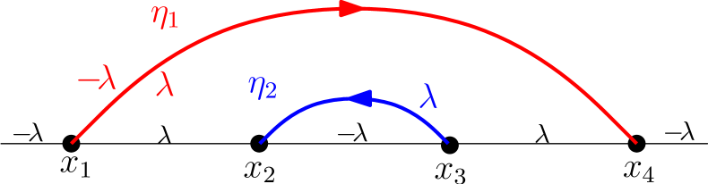
(a) Case $\vbox{\hbox{\includegraphics[scale={0.3}]{figures/link-2.pdf}}}=\{\{1,4\},\{2,3\}\}$

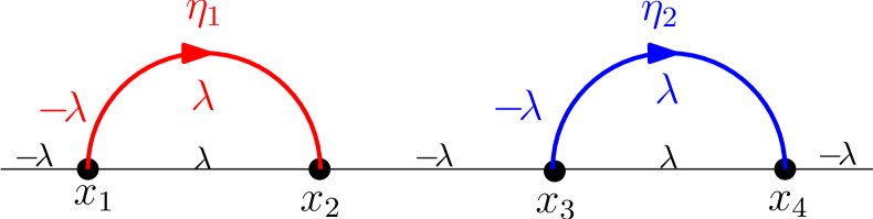
(b) Case $\vbox{\hbox{\includegraphics[scale={0.3}]{figures/link-1.pdf}}}=\{\{1,2\},\{3,4\}\}$.

Figure 5.1: Two level lines of the $\operatorname{GFF}$. The conditional law of $\eta_{1}$ given $\eta_{2}$ is the chordal $\operatorname{SLE}_{4}$ and the conditional law of $\eta_{2}$ given $\eta_{1}$ is the chordal $\operatorname{SLE}_{4}$.

Remark 5.1.

The following trivial fact will be important later: For $x_{1}<x_{2}<x_{3}<x_{4}$, we have

$$0\leq\frac{(x_{4}-x_{1})(x_{3}-x_{2})}{(x_{4}-x_{2})(x_{3}-x_{1})}\leq 1.$$

Lemma 5.2.

Set $\vbox{\hbox{\includegraphics[scale={0.3}]{figures/link-2.pdf}}}=\{\{1,4\},\{2,3\}\}$ and $\vbox{\hbox{\includegraphics[scale={0.3}]{figures/link-1.pdf}}}=\{\{1,2\},\{3,4\}\}$. Let $P_{\vbox{\hbox{\includegraphics[scale={0.2}]{figures/link-2.pdf}}}}$ (resp. $P_{\vbox{\hbox{\includegraphics[scale={0.2}]{figures/link-1.pdf}}}}$) be the probability for Case (resp. Case ), as in Figure 5.1. Then we have

$$P_{\vbox{\hbox{\includegraphics[scale={0.2}]{figures/link-2.pdf}}}}=\frac{(x_{4}-x_{3})(x_{2}-x_{1})}{(x_{4}-x_{2})(x_{3}-x_{1})}\qquad\qquad\text{and}\qquad\qquad P_{\vbox{\hbox{\includegraphics[scale={0.2}]{figures/link-1.pdf}}}}=1-P_{\vbox{\hbox{\includegraphics[scale={0.2}]{figures/link-2.pdf}}}}=\frac{(x_{4}-x_{1})(x_{3}-x_{2})}{(x_{4}-x_{2})(x_{3}-x_{1})}.$$

Proof.

We know that $\eta:=\eta_{1}$ is an $\operatorname{SLE}_{4}(-2,+2,-2)$ process with force points $(x_{2},x_{3},x_{4})$. If $T$ is the continuation threshold of $\eta$, then Case corresponds to $\{\eta(T)=x_{4}\}$ and Case to $\{\eta(T)=x_{2}\}$. Let $(W_{t},0\leq t\leq T)$ be the Loewner driving function of $\eta$ and $(g_{t},0\leq t\leq T)$ the corresponding conformal maps. Define, for $t<T$,

$$M_{t}:=\frac{(g_{t}(x_{4})-W_{t})(g_{t}(x_{3})-g_{t}(x_{2}))}{(g_{t}(x_{4})-g_{t}(x_{2}))(g_{t}(x_{3})-W_{t})}.$$

Using Itô’s formula, one can check that $M_{t}$ is a local martingale, and it is bounded by Remark 5.1: we have $0\leq M_{t}\leq 1$, for $t<T$. Moreover, by Lemma B.2 of Appendix B, we have almost surely, as $t\to T$,

$$M_{t}\to 1, \quad\text{when }\eta(t)\to x_{2}\qquad\text{and}\qquad M_{t}\to 0,\quad\text{when }\eta(t)\to x_{4}.$$

Therefore, the optional stopping theorem implies that

$$P_{\vbox{\hbox{\includegraphics[scale={0.2}]{figures/link-1.pdf}}}}=\mathbb{P}[\eta(T)=x_{2}]=\mathbb{E}\left[M_{T}\right]=M_{0}=\frac{(x_{4}-x_{1})(x_{3}-x_{2})}{(x_{4}-x_{2})(x_{3}-x_{1})}.$$

The formula for the probability $P_{\vbox{\hbox{\includegraphics[scale={0.2}]{figures/link-2.pdf}}}}$ then follows by a direct calculation. ∎

5.3 Connection Probabilities for Level Lines

Fix $N\geq 2$ and $x_{1}<\cdots<x_{2N}$. Let $\Gamma$ be the $\operatorname{GFF}$ on $\mathbb{H}$ with alternating boundary data:

$$\lambda\text{ on }(x_{2j-1},x_{2j}),\text{ for }j\in\{1,\ldots,N\},\qquad\text{and}\qquad-\lambda\text{ on }(x_{2j},x_{2j+1}),\text{ for }j\in\{0,1,\ldots,N\},$$

with the convention that $x_{0}=-\infty$ and $x_{2N+1}=\infty$. For $j\in\{1,\ldots,N\}$, let $\eta_{j}$ be the level line of $\Gamma$ starting from $x_{2j-1}$. The possible terminal points of $\eta_{j}$ are the $x_{n}$’s with an even index $n$. The level lines $\eta_{1},\ldots,\eta_{N}$ do not hit each other, so their endpoints form a (planar) link pattern $\mathcal{A}\in\mathrm{LP}_{N}$. In Lemma 5.5, for each $\alpha\in\mathrm{LP}_{N}$, we derive the connection probability $P_{\alpha}:=\mathbb{P}[\mathcal{A}=\alpha]$. To this end, we use the next lemmas, which relate martingales for level lines with solutions of the system $\mathrm{(PDE)}$ (1.1) with $\kappa=4$.

Lemma 5.3.

Let $\eta=\eta_{1}$ be the level line of $\Gamma$ starting from $x_{1}$, let $W_{t}$ be its driving function, and $(g_{t},t\geq 0)$ the corresponding family of conformal maps. Denote $X_{j1}:=g_{t}(x_{j})-W_{t}$ and $X_{ji}:=g_{t}(x_{j})-g_{t}(x_{i})$, for $i,j\in\{2,\ldots,2N\}$. For any subset $S\subset\{1,\ldots,2N\}$ containing $1$, define

$$M_{t}^{(S)}:=\prod_{1\leq i<j\leq 2N}X_{ji}^{\delta(i,j)},\qquad\text{where }\quad\delta(i,j)=\begin{cases}0,&\text{if }i,j\in S,\text{ or }i,j\not\in S,\\ (-1)^{1+i+j},&\text{if }i\in S\text{ and }j\not\in S,\text{or }i\not\in S\text{ and }j\in S.\end{cases}$$

Then, $M_{t}^{(S)}$ is a local martingale.

We remark that the local martingale $M^{(S)}$ in Lemma 5.3 is in fact the Radon-Nikodym derivative between the law of $\eta$ (i.e., the level line of the $\operatorname{GFF}$ with alternating boundary data), and the law of a level line of the $\operatorname{GFF}$ with a different boundary data — see the discussion in Section 6.4.

Proof.

The level line $\eta$ is an $\operatorname{SLE}_{4}(-2,+2,\ldots,-2)$ process with force points $(x_{2},\ldots,x_{2N})$. We recall from (5.1) that its driving function satisfies the SDE

$$\mathrm{d}W_{t}=2\mathrm{d}B_{t}+\sum_{i=2}^{2N}\frac{-\rho_{i}\mathrm{d}t}{g_{t}(x_{i})-W_{t}},\qquad\text{ where }\quad\rho_{i}=2(-1)^{i+1}$$ (5.2)

and $g_{t}$ is the Loewner map. We rewrite $M_{t}^{(S)}$ as follows:

$$M_{t}^{(S)}=\prod_{j=2}^{2N}X_{j1}^{\delta_{j}}\prod_{2\leq i<j\leq 2N}X_{ji}^{\delta(i,j)},\qquad\text{where }\quad\delta_{j}=\delta(1,j).$$

By Itô’s formula, we have

$$\frac{\mathrm{d}M_{t}^{(S)}}{M_{t}^{(S)}}=\; \sum_{j=2}^{2N}\frac{\delta_{j}}{X_{j1}}\left(\frac{2\mathrm{d}t}{X_{j1}}-\mathrm{d}W_{t}\right)\,+\sum_{2\leq i<j\leq 2N}\frac{\delta(i,j)}{X_{ji}}\left(\frac{2\mathrm{d}t}{X_{j1}}-\frac{2\mathrm{d}t}{X_{i1}}\right)$$

$$+\,\sum_{j=2}^{2N}\frac{2\delta_{j}(\delta_{j}-1)\mathrm{d}t}{X_{j1}^{2}}\,+\sum_{2\leq i<j\leq 2N}\frac{4\delta_{i}\delta_{j}\mathrm{d}t}{X_{j1}X_{i1}}$$

$$=\; \sum_{j=2}^{2N}\frac{2\delta_{j}^{2}\mathrm{d}t}{X_{j1}^{2}}+\,\sum_{j=2}^{2N}\sum_{i=2}^{2N}\frac{\delta_{j}\rho_{i}\mathrm{d}t}{X_{j1}X_{i1}}\,+\sum_{2\leq i<j\leq 2N}\left(\frac{-2\delta(i,j)+4\delta_{i}\delta_{j}}{X_{j1}X_{i1}}\right)\mathrm{d}t-\,\sum_{j=2}^{2N}\frac{2\delta_{j}\mathrm{d}B_{t}}{X_{j1}}.$$

For any $S$ containing $1$, the coefficient of the term $\mathrm{d}t/X_{j1}^{2}$ for $j\in\{2,\ldots,2N\}$ is

$$2\delta_{j}^{2}+\delta_{j}\rho_{j}=0,$$

and the coefficient of the term $\mathrm{d}t/(X_{j1}X_{i1})$, for $i,j\in\{2,\ldots,2N\}$, with $i<j$, is

$$\delta_{j}\rho_{i}+\delta_{i}\rho_{j}-2\delta(i,j)+4\delta_{i}\delta_{j}=0.$$

Therefore, $M_{t}^{(S)}$ is a local martingale. ∎

Lemma 5.4.

Let $\eta=\eta_{1}$ be the level line of $\Gamma$ starting from $x_{1}$, let $(W_{t},t\geq 0)$ be its driving function, and $(g_{t},t\geq 0)$ the corresponding family of conformal maps. For a smooth function $\mathcal{U}\colon\mathfrak{X}_{2N}\to\mathbb{R}$, the ratio

$$M_{t}(\mathcal{U}):=\frac{\mathcal{U}(W_{t},g_{t}(x_{2}),\ldots,g_{t}(x_{2N}))}{\mathcal{Z}^{(N)}_{\operatorname{GFF}}(W_{t},g_{t}(x_{2}),\ldots,g_{t}(x_{2N}))}$$

is a local martingale if and only if $\mathcal{U}$ satisfies $\mathrm{(PDE)}$ (1.1) with $i=1$ and $\kappa=4$.

Proof.

Recall the SDE (5.2) for $W_{t}$. Lemma 4.14 gives an explicit formula for the function $\mathcal{Z}:=\mathcal{Z}^{(N)}_{\operatorname{GFF}}$. Using this, one verifies that $\mathcal{Z}$ satisfies the following differential equation: for $\boldsymbol{x}=(x_{1},\ldots,x_{2N})\in\mathfrak{X}_{2N}$,

$$\bigg{(}4\partial_{1}+\sum_{j=2}^{2N}\frac{\rho_{j}}{x_{j}-x_{1}}\bigg{)}\mathcal{Z}(\boldsymbol{x})=0.$$ (5.3)

Furthermore, $\mathcal{Z}$ satisfies $\mathrm{(PDE)}$ (1.1) with $i=1$ and $\kappa=4$:

$$\mathcal{D}^{(1)}\mathcal{Z}(\boldsymbol{x})=0,\qquad\qquad\text{where }\quad\mathcal{D}^{(1)}:=2\partial_{1}^{2}+\sum_{j=2}^{2N}\left(\frac{2\partial_{j}}{x_{j}-x_{1}}-\frac{1}{2(x_{j}-x_{1})^{2}}\right).$$ (5.4)

We denote $\boldsymbol{Y}:=(W_{t},g_{t}(x_{2}),\ldots,g_{t}(x_{2N}))$, and $X_{j1}:=g_{t}(x_{j})-W_{t}$, and $X_{ji}:=g_{t}(x_{j})-g_{t}(x_{i})$, for $i,j\in\{2,\ldots,2N\}$. By Itô’s formula, any (regular enough) function $F(x_{1},\ldots,x_{2N})$ satisfies

$$\mathrm{d}F(\boldsymbol{Y}) =2\partial_{1}F(\boldsymbol{Y})\,\mathrm{d}B_{t}+\bigg{(}2\partial_{1}^{2}+\sum_{j=2}^{2N}\left(\frac{2\partial_{j}}{X_{j1}}-\frac{\rho_{j}\partial_{1}}{X_{j1}}\right)\bigg{)}F(\boldsymbol{Y})\,\mathrm{d}t$$

$$=2\partial_{1}F(\boldsymbol{Y})\,\mathrm{d}B_{t}+\bigg{(}\mathcal{D}^{(1)}+\sum_{j=2}^{2N}\left(\frac{1}{2X^{2}_{j1}}-\frac{\rho_{j}\partial_{1}}{X_{j1}}\right)\bigg{)}F(\boldsymbol{Y})\,\mathrm{d}t.$$

Combining with (5.3) and (5.4), we see that

$$\frac{\mathrm{d}M_{t}(\mathcal{U})}{M_{t}(\mathcal{U})} =\frac{\mathrm{d}\mathcal{U}(\boldsymbol{Y})}{\mathcal{U}(\boldsymbol{Y})}-\frac{\mathrm{d}\mathcal{Z}(\boldsymbol{Y})}{\mathcal{Z}(\boldsymbol{Y})}+4\left(\frac{\partial_{1}\mathcal{Z}(\boldsymbol{Y})}{\mathcal{Z}(\boldsymbol{Y})}\right)^{2}\mathrm{d}t-4\left(\frac{\partial_{1}\mathcal{U}(\boldsymbol{Y})}{\mathcal{U}(\boldsymbol{Y})}\right)\left(\frac{\partial_{1}\mathcal{Z}(\boldsymbol{Y})}{\mathcal{Z}(\boldsymbol{Y})}\right)\mathrm{d}t$$

$$=\left(\frac{2\partial_{1}\mathcal{U}(\boldsymbol{Y})}{\mathcal{U}(\boldsymbol{Y})}-\frac{2\partial_{1}\mathcal{Z}(\boldsymbol{Y})}{\mathcal{Z}(\boldsymbol{Y})}\right)\mathrm{d}B_{t}+\frac{\mathcal{D}^{(1)}\mathcal{U}(\boldsymbol{Y})}{\mathcal{U}(\boldsymbol{Y})}\mathrm{d}t.$$

This implies that $M_{t}(\mathcal{U})$ is a local martingale if and only if $\mathcal{D}^{(1)}\mathcal{U}=0$. ∎

Now, we give the formula for the connection probabilities for the level lines of the $\operatorname{GFF}$. To emphasize the main idea, we postpone a technical detail, Proposition B.1, to Appendix B.

Lemma 5.5.

We have

$$P_{\alpha}=\frac{\mathcal{Z}_{\alpha}(x_{1},\ldots,x_{2N})}{\mathcal{Z}^{(N)}_{\operatorname{GFF}}(x_{1},\ldots,x_{2N})}>0,\quad\text{ for all }\alpha\in\mathrm{LP}_{N},\qquad\text{where }\quad\mathcal{Z}^{(N)}_{\operatorname{GFF}}:=\sum_{\alpha\in\mathrm{LP}_{N}}\mathcal{Z}_{\alpha},$$ (5.5)

and $\{\mathcal{Z}_{\alpha}\colon\alpha\in\mathrm{LP}\}$ is the collection of functions of Theorem 1.1 with $\kappa=4$.

Proof.

By Theorem 1.1, we have $\mathcal{Z}_{\alpha}>0$ for all $\alpha\in\mathrm{LP}_{N}$, so for all $(x_{1},\ldots,x_{2N})\in\mathfrak{X}_{2N}$, we have

$$0<\frac{\mathcal{Z}_{\alpha}(x_{1},\ldots,x_{2N})}{\mathcal{Z}^{(N)}_{\operatorname{GFF}}(x_{1},\ldots,x_{2N})}\leq 1.$$ (5.6)

We prove the assertion by induction on $N\geq 0$. The initial case $N=0$ is a tautology: $\mathcal{Z}_{\emptyset}=1=\mathcal{Z}^{(0)}_{\operatorname{GFF}}$. Let then $N\geq 1$ and assume that formula (5.5) holds for all $\hat{\alpha}\in\mathrm{LP}_{N-1}$. Let $\alpha\in\mathrm{LP}_{N}$. Without loss of generality, we may assume that $\{1,2\}\in\alpha$. Let $\eta$ be the level line of the $\operatorname{GFF}$ $\Gamma$ starting from $x_{1}$, let $T$ be its continuation threshold, $(W_{t},t\geq 0)$ its driving function, and $(g_{t},t\geq 0)$ the corresponding family of conformal maps. Then by Lemma 5.4,

$$M_{t}(\mathcal{Z}_{\alpha}):=\frac{\mathcal{Z}_{\alpha}(W_{t},g_{t}(x_{2}),\ldots,g_{t}(x_{2N}))}{\mathcal{Z}^{(N)}_{\operatorname{GFF}}(W_{t},g_{t}(x_{2}),\ldots,g_{t}(x_{2N}))}$$

is a local martingale for $t<T$.

As $t\to T$, we know that $\eta(t)\to x_{2n}$ for some $n\in\{1,\ldots,N\}$. First, we consider the case when $\eta(t)\to x_{2}$. On the event $\{\eta(T)=x_{2}\}$, as $t\to T$, we have by Lemma 4.3 almost surely

$$M_{t}(\mathcal{Z}_{\alpha})=\frac{(g_{t}(x_{2})-W_{t})^{1/2}}{(g_{t}(x_{2})-W_{t})^{1/2}}\frac{\mathcal{Z}_{\alpha}(W_{t},g_{t}(x_{2}),\ldots,g_{t}(x_{2N}))}{\mathcal{Z}^{(N)}_{\operatorname{GFF}}(W_{t},g_{t}(x_{2}),\ldots,g_{t}(x_{2N}))}\;\longrightarrow\;\frac{\mathcal{Z}_{\hat{\alpha}}(g_{T}(x_{3}),\ldots,g_{T}(x_{2N}))}{\mathcal{Z}^{(N-1)}_{\operatorname{GFF}}(g_{T}(x_{3}),\ldots,g_{T}(x_{2N}))},$$

where $\hat{\alpha}=\alpha/\{1,2\}$. Next, on the event $\{\eta(T)=x_{2n}\}$, we have almost surely

$$\lim_{t\to T}\frac{\mathcal{Z}_{\alpha}(W_{t},g_{t}(x_{2}),\ldots,g_{t}(x_{2N}))}{\mathcal{Z}_{\operatorname{GFF}}^{(N)}(W_{t},g_{t}(x_{2}),\ldots,g_{t}(x_{2n}))}=0,$$

by the bound (3.9) and Proposition B.1. In summary, we have almost surely

$$M_{T}(\mathcal{Z}_{\alpha}):=\lim_{t\to T}M_{t}(\mathcal{Z}_{\alpha})=\mathbb{1}_{\{\eta(T)=x_{2}\}}\;\frac{\mathcal{Z}_{\hat{\alpha}}(g_{T}(x_{3}),\ldots,g_{T}(x_{2N}))}{\mathcal{Z}_{\operatorname{GFF}}^{(N-1)}(g_{T}(x_{3}),\ldots,g_{T}(x_{2N}))}.$$

On the other hand, by (5.6), $M_{t}(\mathcal{Z}_{\alpha})$ is bounded, so the optional stopping theorem gives

$$\frac{\mathcal{Z}_{\alpha}}{\mathcal{Z}^{(N)}_{\operatorname{GFF}}}=M_{0}(\mathcal{Z}_{\alpha})=\mathbb{E}\left[M_{T}(\mathcal{Z}_{\alpha})\right].$$

Combining this with the induction hypothesis $P_{\hat{\alpha}}=\mathcal{Z}_{\hat{\alpha}}/\mathcal{Z}^{(N-1)}_{\operatorname{GFF}}$, we obtain

$$\frac{\mathcal{Z}_{\alpha}}{\mathcal{Z}^{(N)}_{\operatorname{GFF}}}=\mathbb{E}\left[\mathbb{1}_{\{\eta(T)=x_{2}\}}P_{\hat{\alpha}}(g_{T}(x_{3}),\ldots,g_{T}(x_{2N}))\right].$$ (5.7)

Finally, consider the level lines $(\eta_{1},\ldots,\eta_{N})$ of the $\operatorname{GFF}$ $\Gamma$, where, for each $j$, $\eta_{j}$ is the level line starting from $x_{2j-1}$. Given $\eta:=\eta_{1}$, on the event $\{\eta(T)=x_{2}\}$, the conditional law of $(\eta_{2},\ldots,\eta_{N})$ is that of the level lines of the $\operatorname{GFF}$ $\hat{\Gamma}$ with alternating boundary data, where $\hat{\Gamma}$ is $\Gamma$ restricted to the unbounded component of $\mathbb{H}\setminus\eta$. Thus, we have

$$P_{\alpha}=\mathbb{E}\left[\mathbb{1}_{\{\eta(T)=x_{2}\}}P_{\hat{\alpha}}(g_{T}(x_{3}),\ldots,g_{T}(x_{2N}))\right].$$ (5.8)

Combining (5.7) and (5.8), we obtain $P_{\alpha}=\mathcal{Z}_{\alpha}/\mathcal{Z}^{(N)}_{\operatorname{GFF}}$, which is what we sought to prove. ∎

5.4 Marginal Probabilities and Proof of Theorem 1.4

Next we calculate the probability for one level line of the $\operatorname{GFF}$ to terminate at a given point. Again, we postpone a technical result to Appendix B.

Proposition 5.6.

For $a,b\in\{1,\ldots,2N\}$ such that $a$ is odd and $b$ is even, the probability $P^{(a,b)}$ that the level line of the $\operatorname{GFF}$ starting from $x_{a}$ terminates at $x_{b}$ is given by

$$P^{(a,b)}(x_{1},\ldots,x_{2N})=\prod_{\begin{subarray}{c}1\leq j\leq 2N,\\ j\neq a,b\end{subarray}}\bigg{|}\frac{x_{j}-x_{a}}{x_{j}-x_{b}}\bigg{|}^{(-1)^{j}}.$$

Before proving the proposition, we observe that a special case follows by easy martingale arguments.

Lemma 5.7.

The conclusion in Proposition 5.6 holds for $b=a+1$.

Proof.

To simplify notation, we assume $a=1$; the other cases are similar. The level line $\eta:=\eta_{1}$ started from $x_{1}$ is an $\operatorname{SLE}_{4}(-2,+2,\ldots,-2)$ process with force points $(x_{2},\ldots,x_{2N})$. Let $T$ be the continuation threshold of $\eta$. Define, for $t<T$,

$$M_{t}:=\prod_{j=3}^{2N}\left(\frac{g_{t}(x_{j})-W_{t}}{g_{t}(x_{j})-g_{t}(x_{2})}\right)^{(-1)^{j}}.$$

By Lemma 5.3 with $S=\{1,2\}$, $M_{t}$ is a local martingale. Remark 5.1 gives, for all $j\in\{3,\ldots,2N\}$, that

$$\left(\frac{g_{t}(x_{j+1})-W_{t}}{g_{t}(x_{j+1})-g_{t}(x_{2})}\right)\left(\frac{g_{t}(x_{j})-g_{t}(x_{2})}{g_{t}(x_{j})-W_{t}}\right)\leq 1,$$

so $M_{t}$ is bounded: we have $0\leq M_{t}\leq 1$ for $t<T$. Finally, as $t\to T$, we have almost surely $M_{t}\to 1$ when $\eta(t)\to x_{2}$, and Lemma B.3 of Appendix B shows that $M_{t}\to 0$ when $\eta(t)\to x_{2n}$ for $n\in\{2,\ldots,N\}$. Therefore, the optional stopping theorem implies $P^{(1,2)}=\mathbb{P}[\eta(T)=x_{2}]=\mathbb{E}[M_{T}]=M_{0}$, as desired. ∎

To prove the general case in Proposition 5.6, we use the following lemma.

Lemma 5.8.

For any $N\geq 2$ and $a,b\in\{1,\ldots,2N\}$ with odd $a$ and even $b$, the function ${F^{(a,b)}_{N}\colon\mathfrak{X}_{2N}\to\mathbb{C}}$,

$$F^{(a,b)}_{N}(x_{1},\ldots,x_{2N}):=\mathcal{Z}_{\operatorname{GFF}}^{(N)}(x_{1},\ldots,x_{2N})\prod_{\begin{subarray}{c}1\leq j\leq 2N,\\ j\neq a,b\end{subarray}}\bigg{|}\frac{x_{j}-x_{a}}{x_{j}-x_{b}}\bigg{|}^{(-1)^{j}}$$ (5.9)

belongs to the solution space $\mathcal{S}_{N}$ defined in (2.5).

Proof.

The function $F^{(a,b)}_{N}$ clearly satisfies the bound (2.4). Also, because $\mathcal{Z}_{\operatorname{GFF}}^{(N)}$ satisfies $\mathrm{(COV)}$ (1.2) and the product $\prod_{j}\big{|}\frac{x_{j}-x_{a}}{x_{j}-x_{b}}\big{|}^{(-1)^{j}}$ is conformally invariant, $F^{(a,b)}_{N}$ also satisfies $\mathrm{(COV)}$ (1.2). It remains to show $\mathrm{(PDE)}$ (1.1). Without loss of generality, we may assume $a=1$. Combining Lemmas 5.4 and 5.3 (with $S=\{1,b\}$), we see that $F^{(1,b)}_{N}$ satisfes $\mathrm{(PDE)}$ (1.1) as well. Thus, we indeed have $F^{(1,b)}_{N}\in\mathcal{S}_{N}$. ∎

Proof of Proposition 5.6.

On the one hand, because the function $F^{(a,b)}_{N}$ defined in (5.9) belongs to the space $\mathcal{S}_{N}$ by Lemma 5.8, Proposition 4.5 allows us to write it in the form

$$F^{(a,b)}_{N}=\sum_{\alpha\in\mathrm{LP}_{N}}c_{\alpha}\mathcal{Z}_{\alpha},\qquad\text{where }\quad c_{\alpha}=\mathcal{L}_{\alpha}(F^{(a,b)}_{N}).$$

On the other hand, by the identity (1.7) in Theorem 1.4, we have

$$P^{(a,b)}=\sum_{\alpha\in\mathrm{LP}_{N}\colon\{a,b\}\in\alpha}P_{\alpha}=\sum_{\alpha\in\mathrm{LP}_{N}\colon\{a,b\}\in\alpha}\frac{\mathcal{Z}_{\alpha}}{\mathcal{Z}_{\operatorname{GFF}}^{(N)}}.$$

Thus, it suffices to show that

$$\mathcal{L}_{\alpha}(F^{(a,b)}_{N})=\mathbb{1}\{\{a,b\}\in\alpha\}.$$ (5.10)

Without loss of generality, we assume that $a=1$. We prove (5.10) by induction on $N\geq 1$. It is clear for $N=1$. Assume then that $N\geq 2$ and $\mathcal{L}_{\beta}(F^{(1,b)}_{N-1})=\mathbb{1}\{\{1,b\}\in\beta\}$ for all $\beta\in\mathrm{LP}_{N-1}$ and $b\in\{2,4,\ldots,2N-2\}$. Let $\alpha\in\mathrm{LP}_{N}$ and choose $i$ such that $\{i,i+1\}\in\alpha$. We consider two cases.

• $i,i+1\notin\{1,b\}$: By the property (4.13) of the function $\mathcal{Z}_{\operatorname{GFF}}$, we have, for any $\xi\in(x_{i-1},x_{i+2})$,

  $$\lim_{x_{i},x_{i+1}\to\xi}(x_{i+1}-x_{i})^{1/2}\;F^{(1,b)}_{N}(x_{1},\ldots,x_{2N})$$

  $$=\; \lim_{x_{i},x_{i+1}\to\xi}(x_{i+1}-x_{i})^{1/2}\;\mathcal{Z}_{\operatorname{GFF}}^{(N)}(x_{1},\ldots,x_{2N})\prod_{\begin{subarray}{c}1\leq j\leq 2N,\\ j\neq 1,b\end{subarray}}\bigg{|}\frac{x_{j}-x_{1}}{x_{j}-x_{b}}\bigg{|}^{(-1)^{j}}$$

  $$=\; \mathcal{Z}_{\operatorname{GFF}}^{(N-1)}(x_{1},\ldots,x_{i-1},x_{i+2},\ldots,x_{2N})\prod_{\begin{subarray}{c}1\leq j\leq 2N,\\ j\neq 1,b,i,i+1\end{subarray}}\bigg{|}\frac{x_{j}-x_{1}}{x_{j}-x_{b}}\bigg{|}^{(-1)^{j}}$$

  $$=\; F^{(1,b^{\prime})}_{N-1}(x_{1},\ldots,x_{i-1},x_{i+2},\ldots,x_{2N}),$$

  where $b^{\prime}=b$ if $i>b$ and $b^{\prime}=b-2$ if $i<b$. Thus, choosing an allowable ordering for the links in $\alpha$ in such a way that $\{a_{1},b_{1}\}=\{i,i+1\}$, the induction hypothesis shows that

  $$\mathcal{L}_{\alpha}\big{(}F^{(1,b)}_{N}\big{)}=\mathcal{L}_{\alpha/\{i,i+1\}}\big{(}F^{(1,b^{\prime})}_{N-1}\big{)}=\mathbb{1}\{\{1,b^{\prime}\}\in\alpha/\{i,i+1\}\}=\mathbb{1}\{\{1,b\}\in\alpha\}.$$

• $i\in\{1,b\}$ or $i+1\in\{1,b\}$: Then we necessarily have $\{1,b\}\notin\alpha$. By symmetry, it suffices to treat the case $i=1$. Then we have, for any $\xi\in(x_{1},x_{2})$,

  $$\lim_{x_{1},x_{2}\to\xi}(x_{2}-x_{1})^{1/2}\;F^{(1,b)}_{N}(x_{1},\ldots,x_{2N})$$

  $$=\; \lim_{x_{1},x_{2}\to\xi}(x_{2}-x_{1})^{1/2}\;\mathcal{Z}_{\operatorname{GFF}}^{(N)}(x_{1},\ldots,x_{2N})\prod_{\begin{subarray}{c}1\leq j\leq 2N,\\ j\neq 1,2,b\end{subarray}}\bigg{|}\frac{x_{j}-x_{1}}{x_{j}-x_{b}}\bigg{|}^{(-1)^{j}}\times\bigg{|}\frac{x_{2}-x_{1}}{x_{2}-x_{b}}\bigg{|}\quad=\quad 0.$$

This proves (5.10) and finishes the proof of the lemma. ∎

Collecting the results from this section and Section 5.3, we now prove Theorem 1.4. See 1.4

Proof.

By Lemma 5.5, the connection probabilities $P_{\alpha}:=\mathbb{P}[\mathcal{A}=\alpha]$ are given by (1.7) and they are strictly positive. On the event $\{\mathcal{A}=\alpha\}$, we have $(\eta_{1},\ldots,\eta_{N})\in X_{0}^{\alpha}(\mathbb{H};x_{1},\ldots,x_{2N})$, whose law is a global $N$-$\operatorname{SLE}_{4}$ associated to $\alpha$: for each $j\in\{1,\ldots,N\}$, the conditional law of $\eta_{j}$ given $\{\eta_{1},\ldots,\eta_{j-1},\eta_{j+1},\ldots,\eta_{N}\}$ is that of the level line of the $\operatorname{GFF}$ on $\hat{\Omega}_{j}$ with Dobrushin boundary data, which is that of the chordal $\operatorname{SLE}_{4}$. By the uniqueness of the global $N$-$\operatorname{SLE}_{4}$ [BPW18, Theorem 1.2], this global $N$-$\operatorname{SLE}_{4}$ is the global $N$-$\operatorname{SLE}_{4}$ constructed in Theorem 1.3. Finally, Proposition 5.6 proves (1.8). ∎

6 Pure Partition Functions for Multiple ${\boldsymbol{\operatorname{SLE}_{4}}}$

In the previous section, we solved the connection probabilities for the level lines of the $\operatorname{GFF}$ in terms of the multiple $\operatorname{SLE}_{4}$ pure partition functions. On the other hand, we constructed the multiple $\operatorname{SLE}_{\kappa}$ pure partition functions for all $\kappa\in(0,4]$ in Section 3, see (3.7). The purpose of this section is to give another, algebraic formula for them in the case of $\kappa=4$ (Theorem 1.5, also stated below). This kind of algebraic formulas for connection probabilities were first derived by R. Kenyon and D. Wilson [KW11a, KW11b] in the context of crossing probabilities in discrete models (in a general setup, which includes the loop-erased random walk, $\kappa=2$; and the double-dimer model, $\kappa=4$). In [KKP17], A. Karrila, K. Kytölä, and E. Peltola also studied the scaling limits of connection probabilities of loop-erased random walks and identified them with the multiple $\operatorname{SLE}_{2}$ pure partition functions.

The main virtue of the formula (1.9) in Theorem 1.5 is that for each $\alpha\in\mathrm{LP}_{N}$, it expresses the pure partition function $\mathcal{Z}_{\alpha}$ as a finite sum of well-behaved functions $\mathcal{U}_{\beta}$, for $\beta\in\mathrm{LP}_{N}$, with explicit integer coefficients that enumerate certain combinatorial objects only depending on $\alpha$ and $\beta$ (given in Proposition 2.9). Such combinatorial enumerations have been studied, e.g., in [KW11a, KW11b, KKP17] and they have many desirable properties which can be used in analyzing the pure partition functions. As an example of this, we verify in Section 6.1 that the decay of the rainbow connection probability agrees with the boundary arm exponents (or (half-)watermelon exponents) appearing in the physics literature.

The auxiliary functions $\mathcal{U}_{\alpha}$ implicitly appear in the conformal field theory literature as “conformal blocks” [BPZ84a, FFK89, DFMS97, Rib14, FP19⁺]. In particular, such functions for irrational $\kappa$ are discussed in [KKP19], where properties of them, such as asymptotics analogous to our findings in Lemma 6.6 for $\kappa=4$, are explained in terms of conformal field theory. In Section 6.4, we give a relation between the conformal blocks with $\kappa=4$ and level lines of the $\operatorname{GFF}$.

For each link pattern $\alpha\in\mathrm{LP}_{N}$, we define the conformal block function

$$\mathcal{U}_{\alpha}\colon\mathfrak{X}_{2N}\to\mathbb{R}_{>0}$$

as follows. We write $\alpha$ as an ordered collection (2.11). Then, we set $\vartheta_{\alpha}(i,i):=0$ and

$$\mathcal{U}_{\alpha}(x_{1},\ldots,x_{2N}):= \;\prod_{1\leq i<j\leq 2N}(x_{j}-x_{i})^{\frac{1}{2}\vartheta_{\alpha}(i,j)},$$ (6.1)

$$\text{where }\quad\vartheta_{\alpha}(i,j):=\; \begin{cases}+1,&\text{if }i,j\in\{a_{1},a_{2},\ldots,a_{N}\},\text{ or }i,j\in\{b_{1},b_{2},\ldots,b_{N}\},\\ -1,&\text{otherwise.}\end{cases}$$

When $\alpha=\boldsymbol{\underline{\cap\cap}}_{N}:=\{\{1,2\},\{3,4\},\ldots,\{2N-1,2N\}\}$ is the completely unnested link pattern, the formula (6.1) equals that of the symmetric partition function from Lemma 4.14, so $\mathcal{U}_{\boldsymbol{\underline{\cap\cap}}_{N}}=\mathcal{Z}_{\operatorname{GFF}}^{(N)}$. Also, it follows from Proposition 2.9 that when $\alpha=\boldsymbol{\underline{\Cap}}_{N}:=\{\{1,2N\},\{2,2N-1\},\ldots,\{N-1,N\}\}$ is the rainbow link pattern, then we have $\mathcal{U}_{\boldsymbol{\underline{\Cap}}_{N}}=\mathcal{Z}_{\boldsymbol{\underline{\Cap}}_{N}}$. In general, the conformal block functions $\mathcal{U}_{\alpha}$ and the pure partition functions $\mathcal{Z}_{\alpha}$, for $\alpha\in\mathrm{LP}_{N}$, form two linearly independent sets that are related by a non-trivial change of basis. Theorem 1.5 expresses this change of basis in terms of matrix elements denoted by $\mathcal{M}^{-1}_{\alpha,\beta}$. For illustration, we list some examples of the explicit formulas for $\mathcal{Z}_{\alpha}$ from Theorem 1.5:

• This case is trivial, $\mathcal{Z}_{\vbox{\hbox{\includegraphics[scale={0.2}]{figures/link-0.pdf}}}}(x_{1},x_{2})=(x_{2}-x_{1})^{-1/2}=\mathcal{U}_{\vbox{\hbox{\includegraphics[scale={0.2}]{figures/link-0.pdf}}}}(x_{1},x_{2})$.

• There are two link patterns, and denoting $x_{ji}:=x_{j}-x_{i}$, we have (see also Table 1 in Section 2.4)

  $$\mathcal{Z}_{\vbox{\hbox{\includegraphics[scale={0.2}]{figures/link-2.pdf}}}}(x_{1},x_{2},x_{3},x_{4})\;=\;\; \mathcal{U}_{\vbox{\hbox{\includegraphics[scale={0.2}]{figures/link-2.pdf}}}}(x_{1},x_{2},x_{3},x_{4})\;=\;\left(\frac{x_{43}x_{21}}{x_{41}x_{31}x_{42}x_{32}}\right)^{1/2},$$

  $$\mathcal{Z}_{\vbox{\hbox{\includegraphics[scale={0.2}]{figures/link-1.pdf}}}}(x_{1},x_{2},x_{3},x_{4})\;=\;\; \mathcal{U}_{\vbox{\hbox{\includegraphics[scale={0.2}]{figures/link-1.pdf}}}}(x_{1},x_{2},x_{3},x_{4})\;-\;\mathcal{U}_{\vbox{\hbox{\includegraphics[scale={0.2}]{figures/link-2.pdf}}}}(x_{1},x_{2},x_{3},x_{4})\;=\;\left(\frac{x_{41}x_{32}}{x_{31}x_{21}x_{43}x_{42}}\right)^{1/2}.$$

  Note that these formulas are consistent with Lemma 5.2.

• There are five link patterns, and we have (see also Table 2 in Section 2.4)

  $$\mathcal{Z}_{\vbox{\hbox{\includegraphics[scale={0.2}]{figures/link-7.pdf}}}}\;=\;\; \mathcal{U}_{\vbox{\hbox{\includegraphics[scale={0.2}]{figures/link-7.pdf}}}},$$

  $$\mathcal{Z}_{\vbox{\hbox{\includegraphics[scale={0.2}]{figures/link-6.pdf}}}}\;=\;\; \mathcal{U}_{\vbox{\hbox{\includegraphics[scale={0.2}]{figures/link-6.pdf}}}}\;-\;\mathcal{U}_{\vbox{\hbox{\includegraphics[scale={0.2}]{figures/link-7.pdf}}}},$$

  $$\mathcal{Z}_{\vbox{\hbox{\includegraphics[scale={0.2}]{figures/link-5.pdf}}}}\;=\;\; \mathcal{U}_{\vbox{\hbox{\includegraphics[scale={0.2}]{figures/link-5.pdf}}}}\;-\;\mathcal{U}_{\vbox{\hbox{\includegraphics[scale={0.2}]{figures/link-6.pdf}}}}\;+\;\mathcal{U}_{\vbox{\hbox{\includegraphics[scale={0.2}]{figures/link-7.pdf}}}},$$

  $$\mathcal{Z}_{\vbox{\hbox{\includegraphics[scale={0.2}]{figures/link-4.pdf}}}}\;=\;\; \mathcal{U}_{\vbox{\hbox{\includegraphics[scale={0.2}]{figures/link-4.pdf}}}}\;-\;\mathcal{U}_{\vbox{\hbox{\includegraphics[scale={0.2}]{figures/link-6.pdf}}}}\;+\;\mathcal{U}_{\vbox{\hbox{\includegraphics[scale={0.2}]{figures/link-7.pdf}}}},$$

  $$\mathcal{Z}_{\vbox{\hbox{\includegraphics[scale={0.2}]{figures/link-3.pdf}}}}\;=\;\; \mathcal{U}_{\vbox{\hbox{\includegraphics[scale={0.2}]{figures/link-3.pdf}}}}\;-\;\mathcal{U}_{\vbox{\hbox{\includegraphics[scale={0.2}]{figures/link-4.pdf}}}}\;-\;\mathcal{U}_{\vbox{\hbox{\includegraphics[scale={0.2}]{figures/link-5.pdf}}}}\;+\;\mathcal{U}_{\vbox{\hbox{\includegraphics[scale={0.2}]{figures/link-6.pdf}}}}\;-\;2\,\mathcal{U}_{\vbox{\hbox{\includegraphics[scale={0.2}]{figures/link-7.pdf}}}}.$$

We give now the statement and an outline of the proof for Theorem 1.5:

See 1.5

Remark 6.1.

A direct consequence of Theorems 1.1 and 1.5 is that the right-hand side of (1.9) satisfies the power law bound (1.4) with $\kappa=4$. This is far from clear from the right-hand side of (1.9) itself.

The proof of Theorem 1.5 uses two inputs. First, we verify that the right-hand side of the asserted formula (1.9) satisfies all of the properties of the pure partition functions $\mathcal{Z}_{\alpha}$ with $\kappa=4$: the normalization $\mathcal{Z}_{\emptyset}=1$, bound (2.4), system $\mathrm{(PDE)}$ (1.1), covariance $\mathrm{(COV)}$ (1.2), and asymptotics $\mathrm{(ASY)}$ (1.3). Second, with these properties verified, we invoke the uniqueness Corollary 2.4 to conclude that the right-hand side of (1.9) must be equal to $\mathcal{Z}_{\alpha}$. We give the complete proof in the end of Section 6.3.

We point out that it is not difficult to check the properties $\mathrm{(PDE)}$ (1.1) and $\mathrm{(COV)}$ (1.2) — this is a direct calculation. The main step of the proof is establishing the asymptotics $\mathrm{(ASY)}$ (1.3), which we perform by combinatorial calculations in Section 6.3, using notations and results from Section 2.4. However, before finishing the proof of Theorem 1.5, we discuss an application to (half-)watermelon exponents.

6.1 Decay Properties of Pure Partition Functions with $\kappa=4$

Consider the rainbow link pattern $\boldsymbol{\underline{\Cap}}_{N}$ (see Figure 3.1). We prove now that, when its first $N$ variables (or both the first $N$ and the last $N$ variables) tend together, the decay of the pure partition function $\mathcal{Z}_{\boldsymbol{\underline{\Cap}}_{N}}$ agrees with the predictions from the physics literature for certain surface critical exponents [Car84, DS87, Nie87, Wer04, Wu18], known as boundary arm exponents (or (half-)watermelon exponents).

Proposition 6.2.

The rainbow pure partition function has the following decay as its $N$ first variables tend together:

$$\mathcal{Z}_{\boldsymbol{\underline{\Cap}}_{N}}(\epsilon,2\epsilon,\ldots,N\epsilon,1,2,\ldots,N)\quad\overset{\epsilon\to 0}{\sim}\quad\epsilon^{N(N-1)/4}.$$

The symmetric partition function $\mathcal{Z}_{\operatorname{GFF}}$ has the decay

$$\mathcal{Z}^{(N)}_{\operatorname{GFF}}(\epsilon,2\epsilon,\ldots,N\epsilon,1,2,\ldots,N)\quad\overset{\epsilon\to 0}{\sim}\quad\begin{cases}\epsilon^{-N/4},&\text{if $N$ is even,}\\ \epsilon^{-(N-1)/4},&\text{if $N$ is odd.}\end{cases}$$

Proof.

Theorem 1.5 and Proposition 2.9 show that $\mathcal{Z}_{\boldsymbol{\underline{\Cap}}_{N}}=\mathcal{U}_{\boldsymbol{\underline{\Cap}}_{N}}$. Now, it is clear from the definition (6.1) of $\mathcal{U}_{\boldsymbol{\underline{\Cap}}_{N}}$ as a product that the decay from the first $N$ variables $x_{j}=j\epsilon$, for $j\in\{1,\ldots,N\}$, is $\epsilon^{p}$, where the power can be read off from (6.1): $p=\frac{N(N-1)}{2}\times\frac{1}{2}(+1)=\frac{N(N-1)}{4}$. Similarly, by the formula (4.17) of Lemma 4.14, the decay of the symmetric partition function $\mathcal{Z}_{\operatorname{GFF}}$ is also of type $\epsilon^{p^{\prime}}$. To find out the power, we collect the exponents from the differences of the variables $x_{j}=j\epsilon$ in (4.17), for $j\in\{1,\ldots,N\}$:

$$p^{\prime}=\sum_{1\leq k<l\leq N}\frac{1}{2}(-1)^{l-k}=\frac{1}{2}\sum_{k=1}^{N-1}\sum_{m=1}^{N-k}(-1)^{m}=\begin{cases}-N/4,&\text{if $N$ is even,}\\ -(N-1)/4,&\text{if $N$ is odd.}\end{cases}$$

This proves the asserted decay. ∎

We see from Theorem 1.5 and Proposition 6.2 that for the level lines of the $\operatorname{GFF}$, the connection probability associated to the rainbow link pattern (given in Theorem 1.4) has the decay

$$P_{\boldsymbol{\underline{\Cap}}_{N}}=\frac{\mathcal{Z}_{\boldsymbol{\underline{\Cap}}_{N}}(\epsilon,2\epsilon,\ldots,N\epsilon,1,2,\ldots,N)}{\mathcal{Z}^{(N)}_{\operatorname{GFF}}(\epsilon,2\epsilon,\ldots,N\epsilon,1,2,\ldots,N)}\quad\overset{\epsilon\to 0}{\sim}\quad\epsilon^{\alpha_{N}^{+}},\qquad\text{where }\quad\alpha_{N}^{+}=\begin{cases}N^{2}/4,&\text{if $N$ is even,}\\ (N^{2}-1)/4,&\text{if $N$ is odd.}\end{cases}$$

The exponent $\alpha_{N}^{+}$ agrees with the $\operatorname{SLE}_{4}$ boundary arm exponents derived in [Wu18, Proposition 3.1].

Corollary 6.3.

The rainbow pure partition function has the following decay as both its $N$ first variables and its $N$ last variables tend together:

$$\mathcal{Z}_{\boldsymbol{\underline{\Cap}}_{N}}(\epsilon,2\epsilon,\ldots,N\epsilon,1+\epsilon,1+2\epsilon,\ldots,1+N\epsilon)\quad\overset{\epsilon\to 0}{\sim}\quad\epsilon^{N(N-1)/2}.$$

The symmetric partition function $\mathcal{Z}_{\operatorname{GFF}}$ has the decay

$$\mathcal{Z}^{(N)}_{\operatorname{GFF}}(\epsilon,2\epsilon,\ldots,N\epsilon,1+\epsilon,1+2\epsilon,\ldots,1+N\epsilon)\quad\overset{\epsilon\to 0}{\sim}\quad\begin{cases}\epsilon^{-N/2},&\text{if $N$ is even,}\\ \epsilon^{-(N-1)/2},&\text{if $N$ is odd.}\end{cases}$$

Proof.

Because the two sets $\{\epsilon,2\epsilon,\ldots,N\epsilon\}$ and $\{1+\epsilon,1+2\epsilon,\ldots,1+N\epsilon\}$ of variables tend to $0$ and $1$, respectively, we only have to add up the power-law decay of Proposition 6.2 for both. ∎

6.2 First Properties of Conformal Blocks

Now we verify properties $\mathrm{(PDE)}$ (1.1) and $\mathrm{(COV)}$ (1.2) with $\kappa=4$ for $\mathcal{U}_{\alpha}$.

Lemma 6.4.

The functions $\mathcal{U}_{\alpha}\colon\mathfrak{X}_{2N}\to\mathbb{R}_{>0}$ defined in (6.1) satisfy $\mathrm{(PDE)}$ (1.1) with $\kappa=4$.

Proof.

For notational simplicity, we write $x_{ij}=x_{i}-x_{j}$ and $\boldsymbol{x}=(x_{1},\ldots,x_{2N})\in\mathfrak{X}_{2N}$. We need to show that for fixed $i\in\{1,\ldots,2N\}$, we have

$$2\frac{\partial_{i}^{2}\mathcal{U}_{\alpha}(\boldsymbol{x})}{\mathcal{U}_{\alpha}(\boldsymbol{x})}+\sum_{j\neq i}\left(\frac{2}{x_{ji}}\frac{\partial_{j}\mathcal{U}_{\alpha}(\boldsymbol{x})}{\mathcal{U}_{\alpha}(\boldsymbol{x})}-\frac{1}{2x_{ji}^{2}}\right)=0.$$ (6.2)

The terms with derivatives are

$$2\frac{\partial_{i}^{2}\mathcal{U}_{\alpha}(\boldsymbol{x})}{\mathcal{U}_{\alpha}(\boldsymbol{x})}\,=\;\, \frac{1}{2}\sum_{j,k\neq i}\frac{\vartheta_{\alpha}(i,j)\vartheta_{\alpha}(i,k)}{x_{ij}x_{ik}}\,-\,\sum_{j\neq i}\frac{\vartheta_{\alpha}(i,j)}{x_{ij}^{2}}\qquad\text{and}\qquad\sum_{j\neq i}\frac{2}{x_{ji}}\frac{\partial_{j}\mathcal{U}_{\alpha}(\boldsymbol{x})}{\mathcal{U}_{\alpha}(\boldsymbol{x})}\,=\,\sum_{j\neq i}\frac{1}{x_{ji}}\;\sum_{k\neq j}\frac{\vartheta_{\alpha}(j,k)}{x_{jk}}.$$

Using this, the left-hand side of the PDE (6.2) becomes

$$\frac{1}{2}\sum_{j,k\neq i}\frac{\vartheta_{\alpha}(i,j)\vartheta_{\alpha}(i,k)}{x_{ij}x_{ik}}\,-\,\sum_{j\neq i}\frac{\vartheta_{\alpha}(i,j)}{x_{ij}^{2}}\,+\,\sum_{j\neq i}\frac{1}{x_{ji}}\;\sum_{k\neq j}\frac{\vartheta_{\alpha}(j,k)}{x_{jk}}\,-\,\sum_{j\neq i}\frac{1}{2x_{ji}^{2}}.$$ (6.3)

The last term of (6.3) is canceled by the case $k=j$ in the first term, and the second term of (6.3) is canceled by the case $k=i$ in the third term. We are left with

$$\sum_{j\neq i}\frac{1}{x_{ji}}\;\sum_{k\neq i,j}\left(\frac{\vartheta_{\alpha}(j,k)}{x_{jk}}-\frac{\vartheta_{\alpha}(i,j)\vartheta_{\alpha}(i,k)}{2x_{ik}}\right).$$ (6.4)

For a pair $(j,k)$ such that $j\neq i$ and $k\neq i,j$, combining the terms where $j$ and $k$ are interchanged, we get a term of the form

$$\left(\frac{\vartheta_{\alpha}(j,k)}{x_{ji}x_{jk}}+\frac{\vartheta_{\alpha}(j,k)}{x_{ki}x_{kj}}\right)+\frac{\vartheta_{\alpha}(i,j)\vartheta_{\alpha}(i,k)}{x_{ji}x_{ki}}\;=\;\frac{\vartheta_{\alpha}(j,k)}{x_{ji}x_{ik}}+\frac{\vartheta_{\alpha}(i,j)\vartheta_{\alpha}(i,k)}{x_{ji}x_{ki}}\;=\;\frac{\vartheta_{\alpha}(j,k)-\vartheta_{\alpha}(i,j)\vartheta_{\alpha}(i,k)}{x_{ji}x_{ik}}.$$

It remains to notice that the numbers $\vartheta_{\alpha}$ defined in (6.1) satisfy the identity $\vartheta_{\alpha}(j,k)-\vartheta_{\alpha}(i,j)\vartheta_{\alpha}(i,k)=0$ for all $i,j$, and $k$. This proves (6.2) and finishes the proof. ∎

Lemma 6.5.

The functions $\mathcal{U}_{\alpha}\colon\mathfrak{X}_{2N}\to\mathbb{R}_{>0}$ defined in (6.1) satisfy $\mathrm{(COV)}$ (1.2) with $\kappa=4$.

Proof.

For any conformal map $\varphi\colon\mathbb{H}\to\mathbb{H}$, we have the identity $\frac{\varphi(z)-\varphi(w)}{z-w}=\sqrt{\varphi^{\prime}(z)}\sqrt{\varphi^{\prime}(w)}$ for all $z,w\in\overline{\mathbb{H}}$, see e.g. [KP16, Lemma 4.7]. Using this identity, we calculate

$$\frac{\mathcal{U}_{\alpha}(\varphi(x_{1}),\ldots,\varphi(x_{2N}))}{\mathcal{U}_{\alpha}(x_{1},\ldots,x_{2N})}=\prod_{1\leq i<j\leq 2N}\left(\frac{\varphi(x_{j})-\varphi(x_{i})}{x_{j}-x_{i}}\right)^{\frac{1}{2}\vartheta_{\alpha}(i,j)}=\prod_{1\leq i<j\leq 2N}\big{(}\varphi^{\prime}(x_{j})\varphi^{\prime}(x_{i})\big{)}^{\frac{1}{4}\vartheta_{\alpha}(i,j)}.$$

For each $j\in\{1,\ldots,2N\}$, the factor $\varphi^{\prime}(x_{j})$ comes with the total power $\frac{1}{4}(N(-1)+(N-1)(+1))=-\frac{1}{4}$, which equals $-h=(\kappa-6)/2\kappa$ with $\kappa=4$. Thus, $\mathcal{U}_{\alpha}$ satisfy $\mathrm{(COV)}$ (1.2) with $\kappa=4$. ∎

6.3 Asymptotics of Conformal Blocks and Proof of Theorem 1.5

To finish the proof of Theorem 1.5, we need to calculate the asymptotics of the conformal block functions $\mathcal{U}_{\alpha}$. This proof is combinatorial, relying on results from [KW11a, KW11b, KKP17] discussed in Section 2.4. Recall that we identify link patterns $\alpha\in\mathrm{LP}_{N}$ with the corresponding Dyck paths (2.12).

Lemma 6.6.

The collection $\{\mathcal{U}_{\alpha}\colon\alpha\in\mathrm{DP}\}$ of functions defined in (6.1) satisfy the asymptotics property

$$\lim_{x_{j},x_{j+1}\to\xi}\frac{\mathcal{U}_{\alpha}(x_{1},\ldots,x_{2N})}{(x_{j+1}-x_{j})^{-1/2}}=\; \begin{cases}0,&\text{if }\times_{j}\in\alpha,\\ \mathcal{U}_{\alpha\setminus\wedge^{j}}(x_{1},\ldots,x_{j-1},x_{j+2},\ldots,x_{2N}),&\text{if }\wedge^{j}\in\alpha,\\ \mathcal{U}_{\alpha\setminus\vee_{j}}(x_{1},\ldots,x_{j-1},x_{j+2},\ldots,x_{2N}),&\text{if }\vee_{j}\in\alpha,\end{cases}$$ (6.5)

for any $j\in\{1,\ldots,2N-1\}$ and $\xi\in(x_{j-1},x_{j+2})$.

Proof.

Fix $j\in\{1,\ldots,2N-1\}$. If $\times_{j}\in\alpha$, then either both $j$ and $j+1$ are $a$-type indices with labels $a_{r},a_{s}$, or both are $b$-type indices with labels $b_{r},b_{s}$. In either case, we have $\vartheta_{\alpha}(j,j+1)=1$, so the limit in (6.5) is zero. Assume then that $\wedge^{j}\in\alpha$ (resp. $\vee_{j}\in\alpha$). In this case, we have $j=b_{s}$ and $j+1=a_{r}$ (resp. $j=a_{r}$ and $j+1=b_{s}$) for some $r,s\in\{1,\ldots,N\}$, so $\vartheta_{\alpha}(j,j+1)=-1$. By definition (6.1), we have

$$\mathcal{U}_{\alpha}(x_{1},\ldots,x_{2N})= \;\prod_{1\leq k<l\leq 2N}(x_{l}-x_{k})^{\frac{1}{2}\vartheta_{\alpha}(k,l)}$$

$$= \;(x_{j+1}-x_{j})^{-1/2}\prod_{\begin{subarray}{c}k<l,\\ k,l\neq j,j+1\end{subarray}}(x_{l}-x_{k})^{\frac{1}{2}\vartheta_{\alpha}(k,l)}$$

$$\;\times\prod_{k<j}(x_{j+1}-x_{k})^{\frac{1}{2}\vartheta_{\alpha}(j+1,l)}(x_{j}-x_{k})^{\frac{1}{2}\vartheta_{\alpha}(j,l)}\prod_{l>j+1}(x_{l}-x_{j+1})^{\frac{1}{2}\vartheta_{\alpha}(k,j+1)}(x_{l}-x_{j})^{\frac{1}{2}\vartheta_{\alpha}(k,j)}.$$

The first factor cancels with the normalization factor $(x_{j+1}-x_{j})^{1/2}$ in the limit (6.5). The second product is independent of $x_{j},x_{j+1}$ and tends to $\mathcal{U}_{\alpha\setminus\wedge^{j}}(x_{1},\ldots,x_{j-1},x_{j+2},\ldots,x_{2N})$ in the limit (6.5) (resp. to $\mathcal{U}_{\alpha\setminus\vee_{j}}$). Finally, the products in the last line tend to one in the limit (6.5), because we have $\vartheta_{\alpha}(k,j+1)=-\vartheta_{\alpha}(k,j)$, for all $k<j$, and $\vartheta_{\alpha}(j+1,l)=-\vartheta_{\alpha}(j,l)$, for all $l>j+1$. This proves the lemma. ∎

Lemma 6.7.

The functions defined by the right-hand side of (1.9) satisfy $\mathrm{(ASY)}$ (1.3) with $\kappa=4$.

Proof.

Denote the functions in question by

$$\tilde{\mathcal{Z}}_{\alpha}(x_{1},\ldots,x_{2N}):=\; \sum_{\beta\succeq\alpha}\mathcal{M}^{-1}_{\alpha,\beta}\,\mathcal{U}_{\beta}(x_{1},\ldots,x_{2N}).$$ (6.6)

Fix $j\in\{1,\ldots,2N-1\}$. For the asymptotics property $\mathrm{(ASY)}$ (1.3), we have two cases to consider: either $\{j,j+1\}\in\alpha$ or $\{j,j+1\}\notin\alpha$. As explained in Section 2.4, these can be equivalently written in terms of the Dyck path $\alpha\in\mathrm{DP}_{N}$ as $\wedge^{j}\in\alpha$ and $\wedge^{j}\notin\alpha$. The asserted property $\mathrm{(ASY)}$ (1.3) with $\kappa=4$ can thus be written in the following form: for all $\alpha\in\mathrm{LP}_{N}$, and for all $j\in\{1,\ldots,2N-1\}$ and $\xi\in(x_{j-1},x_{j+2})$, we have

$$\lim_{x_{j},x_{j+1}\to\xi}\frac{\tilde{\mathcal{Z}}_{\alpha}(x_{1},\ldots,x_{2N})}{(x_{j+1}-x_{j})^{-1/2}}=\begin{cases}0,\quad&\text{if }\wedge^{j}\notin\alpha,\\ \tilde{\mathcal{Z}}_{\alpha\setminus\wedge^{j}}(x_{1},\ldots,x_{j-1},x_{j+2},\ldots,x_{2N}),&\text{if }\wedge^{j}\in\alpha.\end{cases}$$ (6.7)

We prove the property (6.7) for $\tilde{\mathcal{Z}}_{\alpha}$ separately in the two cases $\wedge^{j}\in\alpha$ and $\wedge^{j}\notin\alpha$.

Assume first that $\wedge^{j}\notin\alpha$. We split the right-hand side of (6.6) into three sums:

$$\tilde{\mathcal{Z}}_{\alpha}=\sum_{\beta\succeq\alpha\colon\vee_{j}\in\beta}\mathcal{M}^{-1}_{\alpha,\beta}\,\mathcal{U}_{\beta}\,+\sum_{\beta\succeq\alpha\colon\wedge^{j}\in\beta}\mathcal{M}^{-1}_{\alpha,\beta}\,\mathcal{U}_{\beta}\,+\sum_{\beta\succeq\alpha\colon\times_{j}\in\beta}\mathcal{M}^{-1}_{\alpha,\beta}\,\mathcal{U}_{\beta}.$$

Using Lemma 2.10(b), we combine the first and second sums to one sum over $\beta$ such that $\vee_{j}\in\beta$, by replacing $\beta$ in the second sum by $\beta\uparrow\lozenge_{j}$. Furthermore, Lemma 2.10(d) shows that the coefficients in these two sums are related by $\mathcal{M}^{-1}_{\alpha,\beta}=-\mathcal{M}^{-1}_{\alpha,\beta\uparrow\lozenge_{j}}$. Therefore, we obtain

$$\tilde{\mathcal{Z}}_{\alpha}=\sum_{\beta\succeq\alpha\colon\vee_{j}\in\beta}\mathcal{M}^{-1}_{\alpha,\beta}\,\big{(}\mathcal{U}_{\beta}-\mathcal{U}_{\beta\uparrow\lozenge_{j}}\big{)}\,+\sum_{\beta\succeq\alpha\colon\times_{j}\in\beta}\mathcal{M}^{-1}_{\alpha,\beta}\,\mathcal{U}_{\beta}.$$

Now, it follows from Lemma 6.6 that the last sum vanishes in the limit (6.7), and that the functions $\mathcal{U}_{\beta}$ and $\mathcal{U}_{\beta\uparrow\lozenge_{j}}$ have the same limit, so they cancel. In conclusion, the limit (6.7) of $\tilde{\mathcal{Z}}_{\alpha}$ is zero when $\wedge^{j}\notin\alpha$.

Assume then that $\wedge^{j}\in\alpha$. By Proposition 2.9, the system (6.6) with $\alpha\in\mathrm{DP}_{N}$ is invertible, and

$$\mathcal{U}_{\beta}(x_{1},\ldots,x_{2N})=\; \sum_{\alpha\in\mathrm{DP}_{N}}\mathcal{M}_{\beta,\alpha}\,\tilde{\mathcal{Z}}_{\alpha}(x_{1},\ldots,x_{2N}),\qquad\text{for any }\beta\in\mathrm{DP}_{N},$$ (6.8)

where $\mathcal{M}_{\beta,\alpha}=\mathbb{1}\{\beta\stackrel{{\scriptstyle\scriptscriptstyle{()}}}{{\scriptstyle{\longleftarrow}}}\alpha\}$. We already know by the first part of the proof that the limit (6.7) of $\tilde{\mathcal{Z}}_{\alpha}$ is zero when $\wedge^{j}\notin\alpha$. Therefore, taking the the limit (6.7) of the right-hand side of (6.8) gives

$$\;\sum_{\alpha\in\mathrm{DP}_{N}}\mathbb{1}\{\beta\stackrel{{\scriptstyle\scriptscriptstyle{()}}}{{\scriptstyle{\longleftarrow}}}\alpha\}\,\lim_{x_{j},x_{j+1}\to\xi}\frac{\tilde{\mathcal{Z}}_{\alpha}(x_{1},\ldots,x_{2N})}{(x_{j+1}-x_{j})^{-1/2}}$$

$$=\; \sum_{\alpha\colon\wedge^{j}\in\alpha}\mathbb{1}\{\beta\stackrel{{\scriptstyle\scriptscriptstyle{()}}}{{\scriptstyle{\longleftarrow}}}\alpha\}\,\lim_{x_{j},x_{j+1}\to\xi}\frac{\tilde{\mathcal{Z}}_{\alpha}(x_{1},\ldots,x_{2N})}{(x_{j+1}-x_{j})^{-1/2}},\qquad\text{for any }\beta\in\mathrm{DP}_{N}.$$ (6.9)

We want to calculate the limit in (6.9) for any fixed $\alpha\in\mathrm{DP}_{N}$ such that $\wedge^{j}\in\alpha$.

By Lemma 2.10(c), we have $\beta\stackrel{{\scriptstyle\scriptscriptstyle{()}}}{{\scriptstyle{\longleftarrow}}}\alpha$ if and only if $\lozenge_{j}\in\beta$ and $\beta\setminus\lozenge_{j}\stackrel{{\scriptstyle\scriptscriptstyle{()}}}{{\scriptstyle{\longleftarrow}}}\alpha\setminus\wedge^{j}$. Now, choose $\beta\in\mathrm{DP}_{N}$ such that $\wedge^{j}\in\beta$, and denote $\hat{\beta}=\beta\setminus\wedge^{j}$. Then, by Lemma 2.10(c), we have $\mathbb{1}\{\beta\stackrel{{\scriptstyle\scriptscriptstyle{()}}}{{\scriptstyle{\longleftarrow}}}\alpha\}=\mathbb{1}\{\hat{\beta}\stackrel{{\scriptstyle\scriptscriptstyle{()}}}{{\scriptstyle{\longleftarrow}}}\hat{\alpha}\}$ and we can re-index the sum in (6.9) by $\hat{\alpha}=\alpha\setminus\wedge^{j}$, to obtain

$$\sum_{\hat{\alpha}\in\mathrm{DP}_{N-1}}\mathbb{1}\{\hat{\beta}\stackrel{{\scriptstyle\scriptscriptstyle{()}}}{{\scriptstyle{\longleftarrow}}}\hat{\alpha}\}\,\lim_{x_{j},x_{j+1}\to\xi}\frac{\tilde{\mathcal{Z}}_{\alpha}(x_{1},\ldots,x_{2N})}{(x_{j+1}-x_{j})^{-1/2}}.$$ (6.10)

On the other hand, with $\wedge^{j}\in\beta$, Lemma 6.6 gives the limit (6.7) of the left-hand side of (6.8):

$$\frac{\mathcal{U}_{\beta}(x_{1},\ldots,x_{2N})}{(x_{j+1}-x_{j})^{-1/2}}=\; \mathcal{U}_{\hat{\beta}}(x_{1},\ldots,x_{j-1},x_{j+2},\ldots,x_{2N})$$

$$=\; \sum_{\hat{\alpha}\in\mathrm{DP}_{N-1}}\mathbb{1}\{\hat{\beta}\stackrel{{\scriptstyle\scriptscriptstyle{()}}}{{\scriptstyle{\longleftarrow}}}\hat{\alpha}\}\,\tilde{\mathcal{Z}}_{\hat{\alpha}}(x_{1},\ldots,x_{j-1},x_{j+2},\ldots,x_{2N}),$$ (6.11)

where in the last equality we used (6.8) for $\hat{\beta}=\beta\setminus\wedge^{j}$. Combining (6.10) and (6.11), we arrive with

$$\sum_{\hat{\alpha}\in\mathrm{DP}_{N-1}}\mathcal{M}_{\hat{\beta},\hat{\alpha}}\,\lim_{x_{j},x_{j+1}\to\xi}\frac{\tilde{\mathcal{Z}}_{\alpha}(x_{1},\ldots,x_{2N})}{(x_{j+1}-x_{j})^{-1/2}}$$

$$=\; \sum_{\hat{\alpha}\in\mathrm{DP}_{N-1}}\mathcal{M}_{\hat{\beta},\hat{\alpha}}\,\tilde{\mathcal{Z}}_{\hat{\alpha}}(x_{1},\ldots,x_{j-1},x_{j+2},\ldots,x_{2N}),\qquad\text{for any }\hat{\beta}\in\mathrm{DP}_{N-1},$$ (6.12)

where $\mathcal{M}_{\hat{\beta},\hat{\alpha}}=\mathbb{1}\{\hat{\beta}\stackrel{{\scriptstyle\scriptscriptstyle{()}}}{{\scriptstyle{\longleftarrow}}}\hat{\alpha}\}$ and $\alpha\in\mathrm{LP}_{N}$ is determined by $\hat{\alpha}=\alpha\setminus\wedge^{j}$. Recalling that by Proposition 2.9, the system (6.12) is invertible, we can solve for the asserted limit (6.7). This concludes the proof. ∎

Proof of Theorem 1.5.

We first note that the functions defined by the right-hand side of (1.9) satisfy the normalization $\mathcal{Z}_{\emptyset}=1$ and the bound (2.4) — the latter follows immediately from the definition (6.1) of $\mathcal{U}_{\alpha}$, since the coefficients $\mathcal{M}^{-1}_{\alpha,\beta}$ do not depend on the variables $x_{1},\ldots,x_{2N}$. Lemmas 6.4 and 6.5 show that the functions $\mathcal{U}_{\alpha}$ satisfy the properties $\mathrm{(PDE)}$ (1.1) and $\mathrm{(COV)}$ (1.2) with $\kappa=4$, whence the right-hand side of (1.9) also satisfies these properties by linearity. Furthermore, Lemma 6.7 shows that these functions also enjoy the asymptotics property $\mathrm{(ASY)}$ (1.3) of the pure partition functions $\mathcal{Z}_{\alpha}$ with $\kappa=4$. Thus, the uniqueness Corollary 2.4 shows that the right-hand side of (1.9) must be equal to $\mathcal{Z}_{\alpha}$. ∎

6.4 GFF Interpretation

In this final section, we give an interpretation for the functions $\mathcal{U}_{\alpha}$ appearing in Theorem 1.5 as partition functions associated to a particular boundary data of the $\operatorname{GFF}$.

For $\alpha\in\mathrm{LP}_{N}$, recall that we also denote by $\alpha\in\mathrm{DP}_{N}$ the corresponding Dyck path (2.12). Let $\Gamma_{\alpha}$ be the $\operatorname{GFF}$ on $\mathbb{H}$ with the following boundary data:

$$\lambda(2\alpha(k)-1),\quad \text{if }x\in(x_{k},x_{k+1}),\qquad\text{ for all }k\in\{0,1,\ldots,2N\}.$$ (6.13)

Note that by this definition, the boundary value of $\Gamma_{\alpha}$ is always $-\lambda$ on $(-\infty,x_{1})\cup(x_{2N},\infty)$, and $+\lambda$ on $(x_{1},x_{2})\cup(x_{2N-1},x_{2N})$. Define

$$\mathcal{H}_{\alpha}(k):=\lambda(\alpha(k-1)+\alpha(k)-1),\qquad\text{ for all }k\in\{1,2,\ldots,2N\}.$$ (6.14)

Then we always have $\mathcal{H}_{\alpha}(1)=\mathcal{H}_{\alpha}(2N)=0$.

Proposition 6.8.

Let $\alpha\in\mathrm{LP}_{N}$. Let $\Gamma_{\alpha}$ be the $\operatorname{GFF}$ on $\mathbb{H}$ with boundary data given by (6.13). For all $\{a,b\}\in\alpha$, let $\eta_{a}$ (resp. $\eta_{b}$) be the level line of $\Gamma_{\alpha}$ (resp. $-\Gamma_{\alpha}$) with height $\mathcal{H}_{\alpha}(a)$ (resp. $-\mathcal{H}_{\alpha}(b)$) Then, the collection $(\eta_{1},\ldots,\eta_{2N})$ is a local $N$-$\operatorname{SLE}_{4}$ with partition function $\mathcal{U}_{\alpha}$.

Proof.

The collection $(\eta_{1},\ldots,\eta_{2N})$ clearly satisfies the conformal invariance $\mathrm{(CI)}$ and the domain Markov property $\mathrm{(DMP)}$ from the definition of local multiple $\operatorname{SLE}$s in Section 4.2. Thus, we only need to check the marginal law property $\mathrm{(MARG)}$ for each curve. We do this for $\eta_{a}$. On the one hand, as $\eta_{a}$ is the level line of $\Gamma_{\alpha}$ with height $\mathcal{H}_{\alpha}(a)$, its marginal law is an $\operatorname{SLE}_{4}(\underline{\rho})$ with force points $\{x_{1},\ldots,x_{2N}\}\setminus\{x_{a}\}$, where each $x_{a_{j}}$ (resp. $x_{b_{j}}$) is a force point with weight $+2$ (resp. $-2$). Therefore, the driving function $W_{t}$ of $\eta_{a}$ satisfies the SDEs

$$\begin{split}\mathrm{d}W_{t}=\;&2\mathrm{d}B_{t}\,+\,\sum_{i\neq a}\frac{\rho_{i}\mathrm{d}t}{W_{t}-V_{t}^{i}},\qquad\text{where }\quad\rho_{i}=\begin{cases}+2,\quad&\text{if }i\in\{a_{1},\ldots,a_{N}\}\setminus\{a\},\\ -2,&\text{if }i\in\{b_{1},\ldots,b_{N}\}.\end{cases}\\ \mathrm{d}V_{t}^{i}=\;&\frac{2\mathrm{d}t}{V_{t}^{i}-W_{t}},\quad\text{ for }i\neq a,\end{split}$$ (6.15)

where $V_{t}^{i}$ are the time evolutions of the force points $x_{i}$, for $i\neq a$. On the other hand, (6.15) coincides with the SDE system (4.9) of $\mathrm{(MARG)}$ with $F_{j}=2\partial_{a}\log\mathcal{U}_{\alpha}$, since by definition (6.1) of $\mathcal{U}_{\alpha}$, we have

$$4\partial_{a}\log\mathcal{U}_{\alpha}\,=\,\sum_{i\neq a}\frac{2\vartheta_{\alpha}(i,a)}{W_{t}-V_{t}^{i}}\,=\,\sum_{i\neq a}\frac{\rho_{i}}{W_{t}-V_{t}^{i}}.$$

This completes the proof. ∎

Let $\alpha=\boldsymbol{\underline{\cap\cap}}_{N}$ be the completely unnested link pattern. Then, $\Gamma_{\boldsymbol{\underline{\cap\cap}}_{N}}$ is the $\operatorname{GFF}$ on $\mathbb{H}$ with alternating boundary data, $\mathcal{H}_{\boldsymbol{\underline{\cap\cap}}_{N}}(k)=0$, for all $k$, and $\mathcal{U}_{\boldsymbol{\underline{\cap\cap}}_{N}}=\mathcal{Z}_{\operatorname{GFF}}^{(N)}$. This is the situation discussed in Section 5.3. By Theorem 1.4, all connectivities $\beta\in\mathrm{LP}_{N}$ for the level lines of $\Gamma_{\boldsymbol{\underline{\cap\cap}}_{N}}$ have a positive chance.

However, for a general link pattern $\alpha\in\mathrm{LP}_{N}\setminus\{\boldsymbol{\underline{\cap\cap}}_{N}\}$, the boundary data for $\Gamma_{\alpha}$ is more complicated, and its level lines cannot necessarily form all of the different connectivities: only level lines of $\Gamma_{\alpha}$ and level lines of $-\Gamma_{\alpha}$ with respective heights $\mathcal{H}$ and $-\mathcal{H}$ of the same magnitude can connect with each other. For example, when $\alpha=\boldsymbol{\underline{\Cap}}_{N}$, then $\Gamma_{\boldsymbol{\underline{\Cap}}_{N}}$ is the $\operatorname{GFF}$ with the following boundary data:

$$\begin{cases}\lambda(2j-1),\qquad&\text{if }x\in(x_{j},x_{j+1}),\quad\text{for all }j\in\{0,1,\ldots,N\},\\ \lambda(4N-1-2j),\qquad&\text{if }x\in(x_{j},x_{j+1}),\quad\text{for all }j\in\{N+1,N+2,\ldots,2N\},\end{cases}$$

and the heights of the level lines are $\mathcal{H}_{\boldsymbol{\underline{\Cap}}_{N}}(k)=2\lambda(k-1)$, for $k\in\{1,\ldots,N\}$ and $\mathcal{H}_{\boldsymbol{\underline{\Cap}}_{N}}(k)=2\lambda(2N-k)$, for $k\in\{N+1,\ldots,2N\}$. In this case, we have $\mathcal{U}_{\boldsymbol{\underline{\Cap}}_{N}}=\mathcal{Z}_{\boldsymbol{\underline{\Cap}}_{N}}$, and for $j\in\{1,\ldots,N\}$, the curve $\eta_{j}$ merges with $\eta_{2N+1-j}$ almost surely, that is, the level lines necessarily form the rainbow connectivity $\boldsymbol{\underline{\Cap}}_{N}$. The marginal law of $\eta_{1}$ is the $\operatorname{SLE}_{4}(+2,\ldots,+2,-2,\ldots,-2)$ in $\mathbb{H}$ from $x_{1}$ to $x_{2N}$ with force points $(x_{2},\ldots,x_{2N-1})$, where $x_{k}$ (resp. $x_{l}$) is a force point with weight $+2$ for $k\leq N$ (resp. with weight $-2$ for $l\geq N+1$).

Remark 6.9.

For each link pattern $\alpha\in\mathrm{LP}_{N}$, we associate a balanced subset $S(\alpha)\subset\{1,\ldots,2N\}$ (that is, a subset containing equally many even and odd indices) as follows. Write $\alpha=\{\{a_{1},b_{1}\},\ldots,\{a_{N},b_{N}\}\}$ as an ordered collection as in (2.11). Define

$$S(\alpha):=\{a_{r}\;\colon\;r\in\{1,\ldots,N\}\text{ and }a_{r}\text{ is odd }\}\cup\{b_{s}\;\colon\;s\in\{1,\ldots,N\}\text{ and }b_{s}\text{ is even }\}.$$

Let $\Gamma$ be the $\operatorname{GFF}$ on $\mathbb{H}$ with alternating boundary data. Then the probability that the level lines of $\Gamma$ connect the points with indices in $S(\alpha)$ among themselves and the points with indices in the complement $\{1,2,\ldots,2N\}\setminus S(\alpha)$ among themselves equals

$$\frac{\mathcal{U}_{\alpha}(x_{1},\ldots,x_{2N})}{\mathcal{Z}_{\operatorname{GFF}}^{(N)}(x_{1},\ldots,x_{2N})}.$$

This fact was proved in [KW11a] for interfaces in the double-dimer model. The corresponding claim for the level lines of the $\operatorname{GFF}$ can be proved similarly.

Appendix A Properties of Bound Functions

We first recall the definition of the bound functions: we set $\mathcal{B}_{\emptyset}:=1$ and, for all $\alpha\in\mathrm{LP}_{N}$ and for all nice polygons $(\Omega;x_{1},\ldots,x_{2N})$, we define

$$\mathcal{B}_{\alpha}(\Omega;x_{1},\ldots,x_{2N}):=\prod_{\{a,b\}\in\alpha}H_{\Omega}(x_{a},x_{b})^{1/2}.$$

We also note that, by the monotonicity property (2.3) of the boundary Poisson kernel, for any sub-polygon $(U;x_{1},\ldots,x_{2N})$ we have the inequality

$$\mathcal{B}_{\alpha}(U;x_{1},\ldots,x_{2N})\leq\mathcal{B}_{\alpha}(\Omega;x_{1},\ldots,x_{2N}).$$ (A.1)

Then we collect some useful properties of the functions $\mathcal{B}_{\alpha}$ with $\Omega=\mathbb{H}$:

$$\mathcal{B}_{\alpha}\colon\mathfrak{X}_{2N}\to\mathbb{R}_{>0},\qquad\qquad \mathcal{B}_{\alpha}(x_{1},\ldots,x_{2N}):=\prod_{\{a,b\}\in\alpha}|x_{b}-x_{a}|^{-1}.$$ (A.2)

Lemma A.1.

The function $\mathcal{B}_{\alpha}$ satisfies the following asymptotics: with $\hat{\alpha}=\alpha/\{j,j+1\}$, we have

$$\lim_{\begin{subarray}{c}\tilde{x}_{j},\tilde{x}_{j+1}\to\xi,\\ \tilde{x}_{i}\to x_{i}\text{ for }i\neq j,j+1\end{subarray}}\frac{\mathcal{B}_{\alpha}(\tilde{x}_{1},\ldots,\tilde{x}_{2N})}{(\tilde{x}_{j+1}-\tilde{x}_{j})^{-1}}=\begin{cases}0,\quad&\text{if }\{j,j+1\}\notin\alpha,\\ \mathcal{B}_{\hat{\alpha}}(x_{1},\ldots,x_{j-1},x_{j+2},\ldots,x_{2N}),&\text{if }\{j,j+1\}\in\alpha,\end{cases}$$

for all $\alpha\in\mathrm{LP}_{N}$, and for all $j\in\{1,\ldots,2N-1\}$ and $x_{1}<\cdots<x_{j-1}<\xi<x_{j+2}<\cdots<x_{2N}$.

Proof.

This follows immediately from the definition (A.2). ∎

Then we define, for all $N\geq 1$, the functions

$$\mathcal{B}^{(N)}\colon\mathfrak{X}_{2N}\to\mathbb{R}_{>0},\qquad\qquad \mathcal{B}^{(N)}(x_{1},\ldots,x_{2N}):=\prod_{1\leq k<l\leq 2N}(x_{l}-x_{k})^{(-1)^{l-k}}.$$ (A.3)

We note the connection with the symmetric partition function $\mathcal{Z}_{\operatorname{GFF}}$ for $\kappa=4$ defined in Lemma 4.14:

$$\mathcal{B}^{(N)}(x_{1},\ldots,x_{2N})=\mathcal{Z}_{\operatorname{GFF}}^{(N)}(x_{1},\ldots,x_{2N})^{2}.$$

Also, for a nice polygon $(\Omega;x_{1},\ldots,x_{2N})$, we define

$$\mathcal{B}^{(N)}(\Omega;x_{1},\ldots,x_{2N}):=\prod_{i=1}^{2N}|\varphi^{\prime}(x_{i})|\times\mathcal{B}^{(N)}(\varphi(x_{1}),\ldots,\varphi(x_{2N})),$$

where $\varphi\colon\Omega\to\mathbb{H}$ is any conformal map such that $\varphi(x_{1})<\cdots<\varphi(x_{2N})$.

Lemma A.2.

For all $n\in\{1,\ldots,N\}$ and $\xi<x_{2n+1}<\cdots<x_{2N}$, we have

$$\lim_{\begin{subarray}{c}\tilde{x}_{1},\ldots,\tilde{x}_{2n}\to\xi,\\ \tilde{x}_{i}\to x_{i}\text{ for }2n<i\leq 2N\end{subarray}}\frac{\mathcal{B}^{(N)}(\tilde{x}_{1},\ldots,\tilde{x}_{2N})}{\mathcal{B}^{(n)}(\tilde{x}_{1},\ldots,\tilde{x}_{2n})}=\mathcal{B}^{(N-n)}(x_{2n+1},\ldots,x_{2N}).$$

Proof.

This follows immediately from the definition (A.3). ∎

Appendix B Technical Lemmas

In this appendix, we prove useful results of technical nature. The main result is the next proposition, which we prove in the end of the appendix.

Proposition B.1.

Let $\alpha\in\mathrm{LP}_{N}$ and suppose that $\{1,2\}\in\alpha$. Fix an index $n\in\{2,\ldots,N\}$ and real points $x_{1}<\cdots<x_{2N}$. Suppose $\eta$ is a continuous simple curve in $\mathbb{H}$ starting from $x_{1}$ and terminating at $x_{2n}$ at time $T$, which hits $\mathbb{R}$ only at $\{x_{1},x_{2n}\}$. Let $(W_{t},0\leq t\leq T)$ be its Loewner driving function and $(g_{t},0\leq t\leq T)$ the corresponding conformal maps. Then we have

$$\lim_{t\to T}\frac{\mathcal{B}_{\alpha}(W_{t},g_{t}(x_{2}),\ldots,g_{t}(x_{2N}))}{\mathcal{B}^{(N)}(W_{t},g_{t}(x_{2}),\ldots,g_{t}(x_{2N}))}=0.$$ (B.1)

For the proof, we need a few lemmas.

Lemma B.2.

Let $x_{1}<x_{2}<x_{3}<x_{4}$. Suppose $\eta$ is a continuous simple curve in $\mathbb{H}$ starting from $x_{1}$ and terminating at $x_{4}$ at time $T$, which hits $\mathbb{R}$ only at $\{x_{1},x_{4}\}$. Let $(W_{t},0\leq t\leq T)$ be its Loewner driving function and $(g_{t},0\leq t\leq T)$ the corresponding conformal maps. Define, for $t<T$,

$$\Delta_{t}:=\frac{(g_{t}(x_{4})-W_{t})(g_{t}(x_{3})-g_{t}(x_{2}))}{(g_{t}(x_{4})-g_{t}(x_{2}))(g_{t}(x_{3})-W_{t})}.$$

Then we have $0\leq\Delta_{t}\leq 1$, for all $t<T$, and $\Delta_{t}\to 0$ as $t\to T$.

Proof.

The bound $0\leq\Delta_{t}\leq 1$ follows from Remark 5.1 and the fact that $W_{t}<g_{t}(x_{2})<g_{t}(x_{3})<g_{t}(x_{4})$. It remains to check the limit of $\Delta_{t}$ as $t\to T$. To simplify notations, we denote $g_{t}(x_{2})-W_{t}$ by $X_{21}$ and $g_{t}(x_{3})-g_{t}(x_{2})$ by $X_{32}$, and $g_{t}(x_{4})-g_{t}(x_{3})$ by $X_{43}$. Then we have

$$\Delta_{t}=\frac{(X_{43}+X_{32}+X_{21})X_{32}}{(X_{43}+X_{32})(X_{32}+X_{21})}=\frac{X_{32}/X_{21}+X_{32}/X_{43}+X_{32}^{2}/(X_{21}X_{43})}{1+X_{32}/X_{21}+X_{32}/X_{43}+X_{32}^{2}/(X_{21}X_{43})}.$$

To show that $\Delta_{t}\to 0$ as $t\to T$, it suffices to show that

$$X_{32}/X_{21}\to 0\qquad\text{and}\qquad X_{32}/X_{43}\to 0.$$ (B.2)

For $z\in\mathbb{C}$, denote by $\mathbb{P}^{z}$ the law of Brownian motion in $\mathbb{C}$ started from $z$. Let $\tau$ be the first time when $B$ exits $\mathbb{H}\setminus\eta[0,t]$. Then by [Law05, Remark 3.50], we have

$$X_{43}=\lim_{y\to\infty}y\,\mathbb{P}^{yi}[B_{\tau}\in(x_{3},x_{4})],\qquad X_{32}=\lim_{y\to\infty}y\,\mathbb{P}^{yi}[B_{\tau}\in(x_{2},x_{3})],$$

and $X_{21}$ is the same limit of the probability that $B_{\tau}$ belongs the union of the right side of $\eta[0,t]$ and $(x_{1},x_{2})$. Property (B.2) follows from this. ∎

Lemma B.3.

Fix an index $n\in\{2,3,\ldots,N\}$ and real points $x_{1}<\cdots<x_{2n}$. Suppose $\eta$ is a continuous simple curve in $\mathbb{H}$ starting from $x_{1}$ and terminating at $x_{2n}$ at time $T$, which hits $\mathbb{R}$ only at $\{x_{1},x_{2n}\}$. Let $(W_{t},0\leq t\leq T)$ be its Loewner driving function and $(g_{t},0\leq t\leq T)$ the corresponding conformal maps. Then we have

$$\lim_{t\to T}\prod_{j=3}^{2n}\left(\frac{g_{t}(x_{j})-W_{t}}{g_{t}(x_{j})-g_{t}(x_{2})}\right)^{(-1)^{j}}=0.$$

Proof.

For all odd $j\in\{3,5,\ldots,2n-3\}$, Remark 5.1 shows that

$$0\leq\frac{(g_{t}(x_{j})-g_{t}(x_{2}))(g_{t}(x_{j+1})-W_{t})}{(g_{t}(x_{j})-W_{t})(g_{t}(x_{j+1})-g_{t}(x_{2}))}\leq 1.$$

Combining this with Lemma B.2, we see that, when $t\to T$, we have

$$0\leq\prod_{j=3}^{2n}\left(\frac{g_{t}(x_{j})-W_{t}}{g_{t}(x_{j})-g_{t}(x_{2})}\right)^{(-1)^{j}}\leq\;\frac{(g_{t}(x_{2n-1})-g_{t}(x_{2}))(g_{t}(x_{2n})-W_{t})}{(g_{t}(x_{2n-1})-W_{t})(g_{t}(x_{2n})-g_{t}(x_{2}))}\;\longrightarrow\;0.$$

This proves the lemma. ∎

Next, for any $\alpha\in\mathrm{LP}_{N}$ and $n\in\{1,\ldots,N\}$, we define the function

$$F_{\alpha}^{(n)}(x_{1},\ldots,x_{2N}):=\frac{\mathcal{B}_{\alpha}(x_{1},\ldots,x_{2N})}{\mathcal{B}^{(n)}(x_{1},\ldots,x_{2n})}.$$ (B.3)

Lemma B.4.

Let $\alpha\in\mathrm{LP}_{N}$ and suppose that $\{1,2\}\in\alpha$. Then for all $n\in\{1,\ldots,N\}$, with $\hat{\alpha}=\alpha/\{1,2\}$, we have

$$F_{\alpha}^{(n)}(x_{1},x_{2},x_{3},\ldots,x_{2N})=\prod_{j=3}^{2n}\left(\frac{x_{j}-x_{1}}{x_{j}-x_{2}}\right)^{(-1)^{j}}\times F_{\hat{\alpha}}^{(n-1)}(x_{3},x_{4},\ldots,x_{2N}).$$

Proof.

This follows immediately from the definition (B.3) of $F_{\alpha}^{(n)}$. ∎

Lemma B.5.

For any $\alpha\in\mathrm{LP}_{N}$, $n\in\{1,\ldots,N\}$, and $\xi<x_{2n+1}<\cdots<x_{2N}$, we have

$$\limsup_{\begin{subarray}{c}\tilde{x}_{1},\ldots,\tilde{x}_{2n}\to\xi,\\ \tilde{x}_{i}\to x_{i}\text{ for }2n<i\leq 2N\end{subarray}}F_{\alpha}^{(n)}(\tilde{x}_{1},\ldots,\tilde{x}_{2N})<\infty.$$ (B.4)

Proof.

We prove the claim by induction on $N\geq 1$. It is clear for $N=1$, as $F_{\emptyset}^{(0)}=1$. Assume then that

$$\limsup_{\begin{subarray}{c}\tilde{x}_{1},\ldots,\tilde{x}_{2\ell}\to y,\\ \tilde{x}_{i}\to x_{i}\text{ for }2\ell<i\leq 2N-2\end{subarray}}F_{\beta}^{(\ell)}(\tilde{x}_{1},\ldots,\tilde{x}_{2N-2})<\infty$$

holds for all $\beta\in\mathrm{LP}_{N-1}$, $\ell\in\{1,\ldots,N-1\}$, and $y<x_{2\ell+1}<\cdots<x_{2N-2}$. Let $\alpha\in\mathrm{LP}_{N}$, $n\in\{1,\ldots,N\}$, and $\xi<x_{2n+1}<\cdots<x_{2N}$. Choose $j$ such that $\{j,j+1\}\in\alpha$. We consider three cases.

• $j+1\leq 2n$: In this case, by Lemma B.4, we have

  $$F_{\alpha}^{(n)}(\tilde{x}_{1},\ldots,\tilde{x}_{2N})=\prod_{\begin{subarray}{c}1\leq i\leq 2n,\\ i\neq j,j+1\end{subarray}}\bigg{|}\frac{\tilde{x}_{i}-\tilde{x}_{j}}{\tilde{x}_{i}-\tilde{x}_{j+1}}\bigg{|}^{(-1)^{i+j+1}}\times F_{\alpha/\{j,j+1\}}^{(n-1)}(\tilde{x}_{1},\ldots,\tilde{x}_{j-1},\tilde{x}_{j+2},\ldots,\tilde{x}_{2N}).$$

  Using Remark 5.1, we see that if $j$ is odd, then we have

  $$\prod_{\begin{subarray}{c}1\leq i\leq 2n,\\ i\neq j,j+1\end{subarray}}\bigg{|}\frac{\tilde{x}_{i}-\tilde{x}_{j}}{\tilde{x}_{i}-\tilde{x}_{j+1}}\bigg{|}^{(-1)^{i+j+1}}=\prod_{\begin{subarray}{c}1\leq m\leq n,\\ m\neq(j+1)/2\end{subarray}}\bigg{|}\frac{(\tilde{x}_{2m-1}-\tilde{x}_{j+1})(\tilde{x}_{2m}-\tilde{x}_{j})}{(\tilde{x}_{2m-1}-\tilde{x}_{j})(\tilde{x}_{2m}-\tilde{x}_{j+1})}\bigg{|}\leq 1,$$

  and if $j$ is even, then we have

  $$\prod_{\begin{subarray}{c}1\leq i\leq 2n,\\ i\neq j,j+1\end{subarray}}\bigg{|}\frac{\tilde{x}_{i}-\tilde{x}_{j}}{\tilde{x}_{i}-\tilde{x}_{j+1}}\bigg{|}^{(-1)^{i+j+1}}=\;\bigg{|}\frac{(\tilde{x}_{1}-\tilde{x}_{j})(\tilde{x}_{2n}-\tilde{x}_{j+1})}{(\tilde{x}_{1}-\tilde{x}_{j+1})(\tilde{x}_{2n}-\tilde{x}_{j})}\bigg{|}\;\prod_{\begin{subarray}{c}1\leq m<n,\\ m\neq j/2\end{subarray}}\bigg{|}\frac{(\tilde{x}_{2m}-\tilde{x}_{j+1})(\tilde{x}_{2m+1}-\tilde{x}_{j})}{(\tilde{x}_{2m}-\tilde{x}_{j})(\tilde{x}_{2m+1}-\tilde{x}_{j+1})}\bigg{|}\leq 1.$$

  Thus, we have

  $$F_{\alpha}^{(n)}(\tilde{x}_{1},\ldots,\tilde{x}_{2N})\leq F_{\alpha/\{j,j+1\}}^{(n-1)}(\tilde{x}_{1},\ldots,\tilde{x}_{j-1},\tilde{x}_{j+2},\ldots,\tilde{x}_{2N}),$$

  so by the induction hypothesis, $F_{\alpha}^{(n)}$ remains finite in the limit (B.4).

• $j>2n$: In this case, we have

  $$F_{\alpha}^{(n)}(\tilde{x}_{1},\ldots,\tilde{x}_{2N})=(\tilde{x}_{j+1}-\tilde{x}_{j})^{-1}\;F_{\alpha/\{j,j+1\}}^{(n)}(\tilde{x}_{1},\ldots,\tilde{x}_{j-1},\tilde{x}_{j+2},\ldots,\tilde{x}_{2N}),$$

  which by the induction hypothesis remains finite in the limit (B.4).

• $j=2n$: In this case, we have

  $$F_{\alpha}^{(n)}(\tilde{x}_{1},\ldots,\tilde{x}_{2N})= \;\left(\frac{\tilde{x}_{2n}-\tilde{x}_{2n-1}}{\tilde{x}_{2n+1}-\tilde{x}_{2n}}\right)\;\prod_{i=1}^{2n-2}\left(\frac{\tilde{x}_{2n-1}-\tilde{x}_{i}}{\tilde{x}_{2n}-\tilde{x}_{i}}\right)^{(-1)^{i}}$$

  $$\;\times F_{\alpha/\{j,j+1\}}^{(n-1)}(\tilde{x}_{1},\ldots,\tilde{x}_{j-1},\tilde{x}_{j+2},\ldots,\tilde{x}_{2N}).$$

  By Remark 5.1, we have

  $$\prod_{i=1}^{2n-2}\left(\frac{\tilde{x}_{2n-1}-\tilde{x}_{i}}{\tilde{x}_{2n}-\tilde{x}_{i}}\right)^{(-1)^{i}}=\;\prod_{m=1}^{n-1}\frac{(\tilde{x}_{2n}-\tilde{x}_{2m-1})(\tilde{x}_{2n-1}-\tilde{x}_{2m})}{(\tilde{x}_{2n-1}-\tilde{x}_{2m-1})(\tilde{x}_{2n}-\tilde{x}_{2m})}\;\leq\;1.$$

  By the induction hypothesis, the limit (B.4) of $F_{\alpha/\{j,j+1\}}^{(n-1)}$ is finite, so we see that $F_{\alpha}^{(n)}$ also remains finite in the limit (B.4) (in fact, the limit of $F_{\alpha}^{(n)}$ is zero in this case).

This completes the proof. ∎

Proof of Proposition B.1.

Write $\mathcal{B}_{\alpha}/\mathcal{B}^{(N)}=\big{(}\mathcal{B}^{(n)}/\mathcal{B}^{(N)}\big{)}\big{(}\mathcal{B}_{\alpha}/\mathcal{B}^{(n)}\big{)}$. Then, Lemma A.2 shows that in the limit (B.1), we have $\mathcal{B}^{(N)}/\mathcal{B}^{(n)}\to\mathcal{B}^{(N-n)}>0$. Thus, it suffices to show that $F_{\alpha}^{(n)}=\mathcal{B}_{\alpha}/\mathcal{B}^{(n)}\to 0$ in this limit. Indeed, combining Lemmas B.3–B.5, we see that in the limit $t\to T$, we have

$$\frac{\mathcal{B}_{\alpha}(W_{t},g_{t}(x_{2}),\ldots,g_{t}(x_{2N}))}{\mathcal{B}^{(n)}(W_{t},g_{t}(x_{2}),\ldots,g_{t}(x_{2n}))}= \;F_{\alpha}^{(n)}(W_{t},g_{t}(x_{2}),\ldots,g_{t}(x_{2N}))$$

$$= \;\prod_{j=3}^{2n}\left(\frac{g_{t}(x_{j})-W_{t}}{g_{t}(x_{j})-g_{t}(x_{2})}\right)^{(-1)^{j}}\times F_{\hat{\alpha}}^{(n-1)}(g_{t}(x_{3}),\ldots,g_{t}(x_{2N}))\;\longrightarrow\;0,$$

where $\hat{\alpha}=\alpha/\{1,2\}$. This concludes the proof. ∎

References

- [BB03] Michel Bauer and Denis Bernard. Conformal field theories of stochastic Loewner evolutions. Comm. Math. Phys., 239(3):493–521, 2003.
- [BB04] Michel Bauer and Denis Bernard. Conformal transformations and the SLE partition function martingale. Ann. Henri Poincaré, 5(2):289–326, 2004.
- [BBK05] Michel Bauer, Denis Bernard, and Kalle Kytölä. Multiple Schramm-Loewner evolutions and statistical mechanics martingales. J. Stat. Phys., 120(5-6):1125–1163, 2005.
- [BH19] Stéphane Benoist and Clément Hongler. The scaling limit of critical Ising interfaces is . To appear in Ann. Probab., 2019. Preprint in arXiv:1604.06975.
- [BPW18] Vincent Beffara, Eveliina Peltola, and Hao Wu. On the uniqueness of global multiple s. Preprint in arXiv:1801.07699, 2018.
- [BPZ84a] Alexander A. Belavin, Alexander M. Polyakov, and Alexander B. Zamolodchikov. Infinite conformal symmetry in two-dimensional quantum field theory. Nuclear Phys. B, 241(2):333–380, 1984.
- [BPZ84b] Alexander A. Belavin, Alexander M. Polyakov, and Alexander B. Zamolodchikov. Infinite conformal symmetry of critical fluctuations in two dimensions. J. Stat. Phys., 34(5-6):763–774, 1984.
- [CN07] Federico Camia and Charles M. Newman. Critical percolation exploration path and : a proof of convergence. Probab. Theory Related Fields, 139(3-4):473–519, 2007.
- [Car84] John L. Cardy. Conformal invariance and surface critical behavior. Nuclear Phys. B, 240(4):514–532, 1984.
- [Car89] John L. Cardy. Boundary conditions, fusion rules and the Verlinde formula. Nuclear Phys. B, 324(3):581–596, 1989.
- [CDCH+14] Dmitry Chelkak, Hugo Duminil-Copin, Clément Hongler, Antti Kemppainen, and Stanislav Smirnov. Convergence of Ising interfaces to Schramm’s SLE curves. Comptes Rendus Mathematique, 352(2):157–161, 2014.
- [CHI15] Dmitry Chelkak, Clément Hongler, and Konstantin Izyurov. Conformal invariance of spin correlations in the planar Ising model. Ann. of Math., 181(3):1087–1138, 2015.
- [CI13] Dmitry Chelkak and Konstantin Izyurov. Holomorphic spinor observables in the critical Ising model. Comm. Math. Phys., 322(2):303–332, 2013.
- [CS12] Dmitry Chelkak and Stanislav Smirnov. Universality in the Ising model and conformal invariance of fermionic observables. Invent. Math., 189(3):515–580, 2012.
- [DFMS97] Philippe Di Francesco, Pierre Mathieu, and David Sénéchal. Conformal field theory. Springer-Verlag, New York, 1997.
- [DF85] Viktor S. Dotsenko and Vladimir A. Fateev. Four-point correlation functions and the operator algebra in 2D conformal invariant theories with . Nucl. Phys. B, 251:691–734, 1985.
- [Dub06] Julien Dubédat. Euler integrals for commuting SLEs. J. Stat. Phys., 123(6):1183–1218, 2006.
- [Dub07] Julien Dubédat. Commutation relations for Schramm-Loewner evolutions. Comm. Pure Appl. Math., 60(12):1792–1847, 2007.
- [Dub09] Julien Dubédat. SLE and the free field: Partition functions and couplings. J. Amer. Math. Soc., 22(4):995–1054, 2009.
- [Dub15a] Julien Dubédat. SLE and Virasoro representations: Localization. Comm. Math. Phys., 336(2):695–760, 2015.
- [Dub15b] Julien Dubédat. SLE and Virasoro representations: Fusion. Comm. Math. Phys., 336(2):761–809, 2015.
- [DS87] Bertrand Duplantier and Hubert Saleur. Exact critical properties of two-dimensional dense self-avoiding walks. Nuclear Phys. B, 290:291–326, 1987.
- [DS11] Bertrand Duplantier and Scott Sheffield. Liouville quantum gravity and KPZ. Invent. Math., 185(2):333–393, 2011.
- [FFK89] Giovanni Felder, Jürg Fröhlich, and Gerhard Keller. Braid matrices and structure constants for minimal conformal models. Comm. Math. Phys., 124(4):647–664, 1989.
- [FL13] Laurence S. Field and Gregory F. Lawler. Reversed Radial SLE and the Brownian Loop Measure. J. Stat. Phys., 150:1030–1062 (2013)
- [FK15a] Steven M. Flores and Peter Kleban. A solution space for a system of null-state partial differential equations: Part 1. Comm. Math. Phys., 333(1):389–434, 2015.
- [FK15b] Steven M. Flores and Peter Kleban. A solution space for a system of null-state partial differential equations: Part 2. Comm. Math. Phys., 333(1):435–481, 2015.
- [FK15c] Steven M. Flores and Peter Kleban. A solution space for a system of null-state partial differential equations: Part 3. Comm. Math. Phys., 333(2):597–667, 2015.
- [FK15d] Steven M. Flores and Peter Kleban. A solution space for a system of null-state partial differential equations: Part 4. Comm. Math. Phys., 333(2):669–715, 2015.
- [FP19+] Steven M. Flores and Eveliina Peltola. Monodromy invariant CFT correlation functions of first column Kac operators. In preparation.
- [FSK15] Steven M. Flores, Jacob J. H. Simmons, and Peter Kleban. Multiple-SLEκ connectivity weights for rectangles, hexagons, and octagons. Preprint in arXiv:1505.07756, 2015.
- [FSKZ17] Steven M. Flores, Jacob J. H. Simmons, Peter Kleban, and Robert M. Ziff. A formula for crossing probabilities of critical systems inside polygons. J. Phys. A, 50(6):064005, 2017.
- [Fri04] Roland Friedrich. On connections of conformal field theory and stochastic Loewner evolution. Preprint in arXiv:math-ph/0410029, 2004.
- [FK04] Roland Friedrich and Jussi Kalkkinen. On conformal field theory and stochastic Loewner evolution. Nuclear Phys. B, 687(3):279–302, 2004.
- [FW03] Roland Friedrich and Wendelin Werner. Conformal restriction, highest weight representations and SLE. Comm. Math. Phys., 243(1):105–122, 2003.
- [Gra07] Kevin Graham. On multiple Schramm-Loewner evolutions. J. Stat. Mech. Theory Exp., (3):P03008, 21, 2007.
- [HK13] Clément Hongler and Kalle Kytölä. Ising interfaces and free boundary conditions. J. Amer. Math. Soc., 26(4):1107–1189, 2013.
- [HS13] Clément Hongler and Stanislav Smirnov. The energy density in the planar Ising model. Acta Math., 211(2):191–225, 2013.
- [Hör67] Lars Hörmander. Hypoelliptic second-order differential equations. Acta Math., 119:147–171, 1967.
- [Hör90] Lars Hörmander. The analysis of linear partial differential operators I: Distribution theory and Fourier analysis, volume 256 of Grundlehren der mathematischen Wissenschaften. Springer-Verlag, Berlin Heidelberg, second edition, 1990.
- [Izy15] Konstantin Izyurov. Smirnov’s observable for free boundary conditions, interfaces and crossing probabilities. Comm. Math. Phys., 337(1):225–252, 2015.
- [Izy17] Konstantin Izyurov. Critical Ising interfaces in multiply-connected domains. Probab. Theory Related Fields, 167(1):379–415, 2017.
- [JL18] Mohammad Jahangoshahi and Gregory F. Lawler. On the smoothness of the partition function for multiple Schramm-Loewner evolutions. J. Stat. Phys., 173(5):1353–1368, 2018.
- [Ken08] Richard W. Kenyon. Height fluctuations in the honeycomb dimer model. Comm. Math. Phys., 281(3):675–709, 2008.
- [KKP17] Alex Karrila, Kalle Kytölä, and Eveliina Peltola. Boundary correlations in planar LERW and UST. Preprint in arXiv:1702.03261, 2017.
- [KKP19] Alex Karrila, Kalle Kytölä, and Eveliina Peltola. Conformal blocks, -combinatorics, and quantum group symmetry. To appear in Ann. Henri Poincaré D, 2019. Preprint in arXiv:1709.00249.
- [KL05] Michael J. Kozdron and Gregory F. Lawler. Estimates of random walk exit probabilities and application to loop-erased random walk. Electron. J. Probab., 10(44), 1442–1467, 2005.
- [KL07] Michael J. Kozdron and Gregory F. Lawler. The configurational measure on mutually avoiding SLE paths. In Universality and renormalization, volume 50 of Fields Inst. Commun., pages 199–224. Amer. Math. Soc., Providence, RI, 2007.
- [Kon03] Maxim Kontsevich. CFT, , and phase boundaries. Oberwolfach Arbeitstagung, 2003.
- [KP16] Kalle Kytölä and Eveliina Peltola. Pure partition functions of multiple SLEs. Comm. Math. Phys., 346(1):237–292, 2016.
- [KP19] Kalle Kytölä and Eveliina Peltola. Conformally covariant boundary correlation functions with a quantum group. To appear in J. Eur. Math. Soc., 2019. Preprint in arXiv:1408.1384.
- [KS18] Antti Kemppainen and Stanislav Smirnov. Configurations of FK Ising interfaces and hypergeometric SLE. Math. Res. Lett., 25(3):875–889, 2018.
- [KW11a] Richard W. Kenyon and David B. Wilson. Boundary partitions in trees and dimers. Trans. Amer. Math. Soc., 363(3):1325–1364, 2011.
- [KW11b] Richard W. Kenyon and David B. Wilson. Double-dimer pairings and skew Young diagrams. Electron. J. Combin., 18(1):130–142, 2011.
- [Kyt07] Kalle Kytölä. Virasoro module structure of local martingales of SLE variants. Rev. Math. Phys., 19(5):455–509, 2007.
- [Law05] Gregory F. Lawler. Conformally invariant processes in the plane, volume 114 of Mathematical Surveys and Monographs. Amer. Math. Soc., Providence, RI, 2005.
- [Law09a] Gregory F. Lawler. Partition functions, loop measure, and versions of SLE. J. Stat. Phys., 134(5-6):813–837, 2009.
- [Law09b] Gregory F. Lawler. Schramm-Loewner Evolution (SLE), in Statistical Mechanics, S. Sheffield and T. Spencer ed., volume 16 of AMS IAS/Park City Mathematics Series, 2009.
- [Law11] Gregory F. Lawler. Defining SLE in multiply connected domains with the Brownian loop measure. Preprint in arXiv:1108.4364, 2011.
- [LSW03] Gregory F. Lawler, Oded Schramm, and Wendelin Werner. Conformal restriction: the chordal case. J. Amer. Math. Soc., 16(4):917–955 (electronic), 2003.
- [LSW04] Gregory F. Lawler, Oded Schramm, and Wendelin Werner. Conformal invariance of planar loop-erased random walks and uniform spanning trees. Ann. Probab., 32(1B):939–995, 2004.
- [LW04] Gregory F. Lawler and Wendelin Werner. The Brownian loop soup. Probab. Theory Related Fields, 128(4):565–588, 2004.
- [LV17] Jonatan Lenells and Fredrik Viklund. Schramm’s formula and the Green’s function for multiple . Preprint in arXiv:1701.03698, 2017.
- [LV18] Jonatan Lenells and Fredrik Viklund. Asymptotic analysis of Dotsenko-Fateev integrals. Preprint in arXiv:arXiv:1812.07528, 2018.
- [MS16] Jason Miller and Scott Sheffield. Imaginary geometry I: Interacting SLEs. Probab. Theory Related Fields, 164(3-4):553–705, 2016.
- [Nie87] Bernard Nienhuis. Coulomb gas formulation of two-dimensional phase transitions. In C. Domb and J. L. Lebowitz ed., volume 11 of Phase transitions and critical phenomena, pages 1–53. Academic Press, London, 1987.
- [PW18] Eveliina Peltola and Hao Wu. Crossing probabilities of multiple Ising interfaces. Preprint in arXiv:1808.09438, 2018.
- [Rib14] Sylvain Ribault. Conformal field theory on the plane. Preprint in arXiv:1406.4290, 2014.
- [RS05] Steffen Rohde and Oded Schramm. Basic properties of SLE. Ann. of Math., 161(2):883–924, 2005.
- [RY99] Daniel Revuz and Marc Yor. Continuous martingales and Brownian motion, volume 293 of Grundlehren der mathematischen Wissenschaften. Springer-Verlag, Berlin Heidelberg, third edition, 1999.
- [Rud91] Walter Rudin. Functional Analysis. International Series in Pure and Applied Mathematics. McGeaw-Hill, second edition, 1991.
- [Sch00] Oded Schramm. Scaling limits of loop-erased random walks and uniform spanning trees. Israel J. Math., 118:221–288, 2000.
- [SS09] Oded Schramm and Scott Sheffield. Contour lines of the two-dimensional discrete Gaussian free field. Acta Math., 202(1):21–137, 2009.
- [SS13] Oded Schramm and Scott Sheffield. A contour line of the continuum Gaussian free field. Probab. Theory Related Fields, 157(1-2):47–80, 2013.
- [SW05] Oded Schramm and David B. Wilson. SLE coordinate changes. New York J. Math., 11:659–669 (electronic), 2005.
- [SZ12] Keiichi Shigechi and Paul Zinn-Justin. Path representation of maximal parabolic Kazhdan-Lusztig polynomials. J. Pure Appl. Algebra, 216(11):2533–2548, 2012.
- [She07] Scott Sheffield. Gaussian free fields for mathematicians. Probab. Theory Related Fields, 139(3-4):521–541, 2007.
- [Smi01] Stanislav Smirnov. Critical percolation in the plane: conformal invariance, Cardy’s formula, scaling limits. C. R. Acad. Sci. Paris Sér. I Math., 333(3):239–244, 2001.
- [Smi06] Stanislav Smirnov. Towards conformal invariance of lattice models. In International Congress of Mathematicians. Vol. II, pages 1421–1451. Eur. Math. Soc., Zürich, 2006.
- [Smi10] Stanislav Smirnov. Conformal invariance in random cluster models. I. Holomorphic fermions in the Ising model. Ann. of Math., 172(2):1435–1467, 2010.
- [Str08] Daniel W. Stroock. An introduction to partial differential equations for probabilists, volume 112 of Cambridge Studies in Advanced Mathematics. Cambridge University Press, Cambridge, 2008.
- [Tao09] Terence Tao. An epsilon of room, I: Real analysis. Pages from year three of a mathematical blog, volume 117 of Graduate Studies in Mathematics. Amer. Math. Soc., Providence, RI, 2009.
- [Wer04] Wendelin Werner. Girsanov’s transformation for processes, intersection exponents and hiding exponents. Ann. Fac. Sci. Toulouse Math. (6), 13(1):121–147, 2004.
- [Wu17] Hao Wu. Hypergeometric SLE: conformal Markov characterization and applications. Preprint in arXiv:1703.02022, 2017.
- [WW17] Menglu Wang and Hao Wu. Level lines of Gaussian free field I: zero-boundary GFF. Stochastic Process. Appl., 127(4):1045–1124, 2017.
- [Wu18] Hao Wu. Alternating arm exponents for the critical planar Ising model. Ann. Probab., 46(5): 2863–2907, 2018.
- [Zha08a] Dapeng Zhan. Reversibility of chordal SLE. Ann. Probab., 36(4):1472–1494, 2008.
- [Zha08b] Dapeng Zhan. The scaling limits of planar LERW in finitely connected domains. Ann. Probab., 36(2):467–529, 2008.