Lepton flavor violating Higgs boson decays in seesaw models: new discussions

Abstract

The lepton flavor violating decay of the Standard Model-like Higgs boson (LFVHD), $h\rightarrow\mu\tau$, is discussed in seesaw models at the one-loop level. Based on particular analytic expressions of Passarino-Veltman functions, the two unitary and ’t Hooft Feynman gauges are used to compute the branching ratio of LFVHD and compare with results reported recently. In the minimal seesaw (MSS) model, the branching ratio was investigated in the whole valid range $10^{-9}-10^{15}$ GeV of new neutrino mass scale $m_{n_{6}}$. Using the Casas-Ibarra parameterization, this branching ratio enhances with large and increasing $m_{n_{6}}$. But the maximal value can reach only order of $10^{-11}$. Interesting relations of LFVHD predicted by the MSS and inverse seesaw (ISS) model are discussed. The ratio between two LFVHD branching ratios predicted by the ISS and MSS is simply $m^{2}_{n_{6}}\mu^{-2}_{X}$, where $\mu_{X}$ is the small neutrino mass scale in the ISS. The consistence between different calculations is shown precisely from analytical approach.

I Introduction

After the Higgs boson was observed by ATLAS and CMS higgsdicovery , the LFVHD has been searched experimentally exLFVh , where upper bounds for branching ratios (Brs) of the decays $h\rightarrow\mu\tau,e\tau$ are order of $\mathcal{O}(10^{-2})$. Signals of LFVHD at future colliders have been discussed, where sensitivities for detecting these channel decays are shown to be $10^{-5}$ in the near future LFVcol . Up to now, the lepton flavor violating (LFV) decays of the standard-model-like and new Higgs bosons have been investigated in many models beyond the standard model (SM) Apo ; Apo1 ; EArganda ; iseesaw ; e1612.09290 ; moress ; LFVgeneral ; SUSY ; THDL2 ; LFVHDUgauge ; KHHung . Among them, the MSS MSS is the simplest that can explain successfully the recent neutrino data. Naturally, the mixing between different flavor neutrinos leads to many LFV processes from loop corrections. But it predicts very suppressed branching ratios (Br) of LFV decays of charged leptons. Recent studies on the Br of LFVHD were also shown to be very small EArganda . In contrast, the ISS ISSmodel , another simple extension of the SM, predicts much larger values of LFV branching ratios, including those of LFVHD iseesaw ; e1612.09290 . In fact, the Br of LFVHD in the ISS were calculated in many different ways in order to guarantee the consistence of the LFVHD amplitudes.

We stress that understanding the mechanism for generating loop corrections to Brs of LFVHD in simple models like the MSS and ISS is very important for studying LFVHD processes in other complicated models. That is why LFVHD predicted by these two models were discussed in many works, for example Apo ; Apo1 ; EArganda ; iseesaw ; e1612.09290 ; moress . In the ISS, recent results in iseesaw showed that branching ratios of LFVHD increase with increasing values of very heavy neutrino masses when the Casas-Ibarra method ibarra was applied to formulating the Yukawa couplings of heavy neutrinos . But the Brs are always constrained by upper bounds because of the perturbative limit of the Yukawa couplings. Using the mass insertion approximation, a recent study e1612.09290 also calculated the Br of LFVHD in the ISS model in both unitary and ’t Hooft Feynman, where previous results in iseesaw were confirmed to be well consistent in the region of parameters containing large new neutrino mass scale $m_{n_{6}}$. The above discussions indicate that although one-loop contributions in both MSS and ISS arise from the same set of Feynman diagrams, the two models predict very different Br values. The reason is the appearance of a small mass scale $\mu_{X}$ in the ISS, which gives tiny contributions to the heavy neutrino masses, but affects strongly on the neutrino mixing matrix. Hence there should exist simple relations between two expressions of Brs predicted by the two models. These interesting relations were not discussed previously, therefore will be focused in this work. We will show that if $m_{n_{6}}$ is large enough, the ratio between Brs of LFVHD of the ISS and MSS is order of $m^{2}_{n_{6}}\mu^{-2}_{X}$, enough to explain clearly the LFVHD difference between two models.

Regarding the MSS, LFVHD was discussed mainly in ranges of $10^{2}-10^{7}$ GeV Apo ; EArganda , while the valid range of the new neutrino mass scale is from $\mathcal{O}(10^{-9})$ GeV to $\mathcal{O}(10^{15})$ GeV. In addition, a good estimation made in Ref. Apo suggested that the Br may enhance with increasing masses of heavy neutrinos, even when the Casas-Ibarra parameterization is used. We note that this parameterization are now still widely used to investigate the signal of seesaw models at recent colliders SSbound . As a result, possibilities that large Brs of LFVHD may exist in ranges of new neutrino mass scales that were not mentioned previously. Therefore, studies the LFVHD in the whole valid range as well as new approaches to compare well-known results and confirm consistent analytic formulas for calculating Br of LFVHD in seesaw models are still interesting and necessary. These are main scopes of this work. In particular, in order to guarantee the stability of numerical results at very large values of $m_{n_{6}}$, LFVHD processes will be computed using analytic expressions of Passarino-Veltman functions (PV functions) given in ref. LFVHDUgauge . Using a mathematica code based on these functions, we found that it is much easier and more convenient to increase the precision than using available numerical packages such as Looptools looptool . This makes our calculation different from all previous works. In addition, the one-loop contributions to LFVHD in both unitary and ’t Hooft Feynman gauges will be constructed using notations in LFVHDUgauge . Then we cross-check the consistence between total amplitudes calculated in two gauges, and the ones established in previous works Apo ; EArganda ; iseesaw . A detailed checking divergence cancellation will be presented analytically. For the MSS, after showing that Br of LFVHD is suppressed with small $m_{n_{6}}$, we will pay attention mainly to the region with large $m_{n_{6}}$. To guarantee the consistence of our investigation on LFVHD in the MSS, the connection between analytic formulas of LFVHD amplitudes in the two models MSS and ISS will be discussed deeply. In this work, Yukawa couplings of new neutrinos are only investigated following the Casas-Ibarra parameterization ibarra . This parameterization was used to investigate independently LFVHD processes predicted by the MSS and ISS in Refs. EArganda ; iseesaw , where other important properties of LFVHD were presented in details.

Our work is arranged as follows. Sec. II establishes notations and couplings of a general seesaw model needed for studying LFVHD. In Sec. III, we construct LFVHD amplitudes in two unitary and ’t Hooft Feynman gauges using notations of PV functions given in LFVHDUgauge . Then we prove the divergent cancellation and the consistence between two expressions of the LFVHD amplitudes. In Sec. IV, we show the choice of parameterizing the neutrino mixing matrices. After that, the Brs of LFVHD are numerically investigated. We will focus on new results of LFVHD in the MSS, and interesting relations between the Brs predicted by two models MSS and ISS. Sec. V summarizes new results of this work.

II General formalism and couplings for LFVHD

The general seesaw model is different from the Standard Model (SM) by $K$ additional right-handed neutrinos, $N_{R,I}\sim(1,1,0)$ with $I=1,2,...,K$ numixing . The new Lagrangian part is

$$-\Delta\mathcal{L}=Y_{\nu,aI}\overline{\psi_{L,a}}\widetilde{\phi}N_{R,I}+\frac{1}{2}\overline{(N_{R,I})^{c}}m_{M,IJ}N_{R,J}+\mathrm{h.c.},$$ (1)

where $a=1,2,3$; I,J=1,2,…,K; $\psi_{L,a}=(\nu_{L,a},e_{L,a})^{T}$ are $SU(2)_{L}$ lepton doublets and $(N_{R,I})^{c}=C\overline{N_{R,I}}^{T}$. The Higgs bosons are also doublets $\phi=(G_{W}^{+},(h+iG_{Z}+v)/\sqrt{2})^{T}$ and $\widetilde{\phi}=i\sigma_{2}\phi^{*}$. Each of them consists of three Goldstone bosons of $W^{\pm}$ and $Z$ bosons; a neutral CP-even Higgs boson $h$ and the vacuum expectation value (VEV), $\langle\phi\rangle=\frac{v}{\sqrt{2}}=174$ GeV ($v=246$ GeV). Notations for flavor states of active neutrinos are $\nu_{L}=(\nu_{L,1},\;\nu_{L,2},\;\nu_{L,3})^{T}$ and $(\nu_{L})^{c}\equiv((\nu_{L,1})^{c},\;(\nu_{L,2})^{c},\;(\nu_{L,3})^{c})^{T}$. Notations for new neutrinos are $N_{R}=(N_{R,1},\;N_{R,2},...,\;N_{R,K})^{T}$, and $(N_{R})^{c}=((N_{R,1})^{c},\;(N_{R,2})^{c},...,\;(N_{R,K})^{c})^{T}$. In the bases of the original neutrinos, $\nu^{\prime}_{L}\equiv(\nu_{L},\;(N_{R})^{c})^{T}$ and $(\nu^{\prime}_{L})^{c}=((\nu_{L})^{c},\;N_{R})^{T}$, the Lagrangian part (1) generates the following mass term for neutrinos,

$$-\mathcal{L}^{\nu}_{\mathrm{mass}}\equiv\frac{1}{2}\overline{\nu^{\prime}_{L}}M^{\nu}(\nu^{\prime}_{L})^{c}+\mathrm{h.c.}=\frac{1}{2}\overline{\nu^{\prime}_{L}}\left(\begin{array}[]{cc}0&M_{D}\\ M_{D}^{T}&M_{N}\\ \end{array}\right)(\nu^{\prime}_{L})^{c}+\mathrm{h.c.},$$ (4)

where $M_{N}$ is a symmetric and non-singular $K\times K$ matrix, and $M_{D}$ is a $3\times K$ matrix, $(M_{D})_{aI}=Y_{\nu,aI}\langle\phi\rangle$. The matrix $M^{\nu}$ is symmetric, therefore it can be diagonalized via $(K+3)\times(K+3)$ matrix, $U^{\nu}$, satisfying the unitary condition, $U^{\nu\dagger}U^{\nu}=I$. We define

$$U^{\nu T}M^{\nu}U^{\nu}=\hat{M}^{\nu}=\mathrm{diagonal}(m_{n_{1}},m_{n_{2}},m_{n_{3}},m_{n_{4}},...,m_{n_{(K+3)}}),$$ (5)

where $m_{n_{i}}$ ($i=1,2,...,K+3$) are mass eigenvalues of the $(K+3)$ mass eigenstates $n_{L,i}$, i.e. physical states of neutrinos. Three light active neutrinos are $n_{L,a}$ with $a=1,2,3$. The relation between the flavor and mass eigenstates are

$$\nu^{\prime}_{L}=U^{\nu*}n_{L},\hskip 14.22636pt\mathrm{and}\;(\nu^{\prime}_{L})^{c}=U^{\nu}(n_{L})^{c},$$ (6)

where $n_{L}\equiv(n_{L,1},n_{L,2},...,n_{L,K+3})^{T}$.

In calculation, we will use a general notation of four-component (Dirac) spinor, $n_{i}$ ($i=1,2,..,K+3$), for all active and exotic neutrinos. Specifically, a Majorana fermion $n_{i}$ is defined as $n_{i}\equiv(n_{L,i},\;(n_{L,i})^{c})^{T}=n^{c}_{i}=(n_{i})^{c}$. The chiral components are $n_{L,i}\equiv P_{L}n_{i}$ and $n_{R,i}\equiv P_{R}n_{i}=(n_{L,i})^{c}$, where $P_{L,R}=\frac{1\pm\gamma_{5}}{2}$ are chiral operators. The similar definitions for the original neutrino states are $\nu_{a}\equiv(\nu_{L,a},\;(\nu_{L,a})^{c})^{T}$, $N_{I}\equiv((N_{R,I})^{c},\;N_{R,I})^{T}$, and $\nu^{\prime}=(\nu,\,N)^{T}$. The relations in (6) are rewritten as follows,

$$P_{L}\nu^{\prime}_{i}=\nu^{\prime}_{L,i}=U^{\nu*}_{ij}n_{L,j},\;\mathrm{and}\;P_{R}\nu^{\prime}_{i}=\nu^{\prime}_{R,i}=U^{\nu}_{ij}n_{R,j},\hskip 14.22636pti,j=1,2,...,K+3,$$ (7)

where more precise expressions are $\nu_{L,a}=P_{L}\nu^{\prime}_{a}=U^{\nu*}_{ai}n_{L,i}$, $(N_{R,I})^{c}=P_{L}\nu^{\prime}_{I+3}=U^{\nu*}_{(I+3)j}n_{L,j}$, $(\nu_{L,a})^{c}=P_{R}\nu^{\prime}_{a}=U^{\nu}_{ai}n_{R,i}$, and $N_{R,I}=P_{R}\nu^{\prime}_{I+3}=U^{\nu}_{(I+3)j}n_{R,j}$ ($I=1,2,3,..,K$).

As usual, the covariant derivative is $D_{\mu}=\partial_{\mu}-igT^{a}W^{a}-ig^{\prime}YB_{\mu}$. We emphasize that the signs in $D_{\mu}$ will result in signs of couplings $hG^{\pm}_{W}W^{\pm}$ and $\overline{e}_{a}\nu_{a}W^{-}$. Correspondingly, the lepton flavor violating (LFV) couplings of $W^{\pm}$ boson to leptons are,

$$\mathcal{L}^{\mathrm{lep}}_{\mathrm{kin}}=i\overline{\psi_{L,a}}\gamma^{\mu}D_{\mu}\psi_{L,a} \supset \frac{g}{\sqrt{2}}\left(\overline{\nu_{L,a}}\gamma^{\mu}e_{L,a}W^{+}_{\mu}+\overline{e_{L,a}}\gamma^{\mu}\nu_{L,a}W^{-}_{\mu}\right)$$ (8)

$$= \frac{g}{\sqrt{2}}\left(U^{\nu}_{aj}\overline{n_{j}}\gamma^{\mu}P_{L}e_{a}W^{+}_{\mu}+U^{\nu*}_{aj}\overline{e_{a}}\gamma^{\mu}P_{L}n_{j}W^{-}_{\mu}\right),$$

where $a=1,2,3$; and $j=1,2,...,K+3$.

The Yukawa couplings that contribute to LFVHD are

$$-\mathcal{L}^{\mathrm{lep}}_{\mathrm{Y}} = y_{e_{a}}\overline{\psi_{L,a}}\phi e_{R,a}+Y_{\nu,aI}\overline{\psi_{L,a}}\widetilde{\phi}N_{R,I}+\mathrm{h.c.}$$ (9)

$$\supset \frac{m_{e_{a}}}{v}h\overline{e_{a}}e_{a}+\frac{\sqrt{2}m_{e_{a}}}{v}\left(U^{\nu}_{aj}G^{+}_{W}\overline{n_{L,j}}e_{R,a}+U^{\nu*}_{aj}G^{-}_{W}\overline{e_{R,a}}n_{L,j}\right)$$

$$+ Y_{\nu,aI}\left[-G^{-}_{W}\overline{e_{L,a}}N_{R,I}-G^{+}_{W}\overline{N_{R,I}}e_{L,a}\right]$$

$$+ \frac{1}{v\sqrt{2}}h\left[(M_{D})_{aI}\overline{\nu_{L,a}}N_{R,I}+(M_{D})^{*}_{aI}\overline{N_{R,I}}\nu_{L,a}\right].$$

Using $(M_{D})_{aI}=M^{\nu}_{a(I+3)}$, and $N_{R,I}=\nu^{\prime}_{R,(I+3)}$, the last line in (9) changes in to the new form, $\frac{1}{v}h\overline{n_{i}}\left[M^{\nu}_{a(I+3)}U^{\nu}_{ai}U^{\nu}_{(I+3)j}P_{R}+M^{\nu*}_{a(I+3)}U^{\nu*}_{(I+3)i}U^{\nu*}_{aj}P_{L}\right]n_{j}$. It can be proved that

$$M^{\nu}_{a(I+3)}U^{\nu}_{ai}U^{\nu}_{(I+3)j}P_{R}+M^{\nu*}_{a(I+3)}U^{\nu*}_{(I+3)i}U^{\nu*}_{aj}P_{L}=\left(\sum_{a=1}^{3}U^{\nu}_{ai}U^{\nu*}_{aj}\right)\left(m_{n_{i}}P_{L}+m_{n_{j}}P_{R}\right),$$ (10)

which was given in EArganda ; iseesaw . A proof is as follows, based on the following properties of $M^{\nu}$ and $U^{\nu}$ defined in Eqs. (4) and (5),

$$M^{\nu}_{ab} = 0,\hskip 14.22636ptM^{\nu}_{(I+3)(J+3)}=(m_{N})_{IJ},\hskip 14.22636ptM^{\nu}_{a(I+3)}=(M_{D})_{aI},\hskip 14.22636ptM^{\nu}_{(I+3)a}=(M_{D}^{T})_{Ia},$$

$$U^{\nu\dagger}U^{\nu} = I,\hskip 14.22636ptM^{\nu}=U^{\nu*}\hat{M}^{\nu}U^{\nu\dagger},\hskip 14.22636pt\mathrm{and}\;M^{\nu*}=U^{\nu}\hat{M}^{\nu}U^{\nu T}.$$ (11)

The first term in the left hand side of Eq. (10) will change exactly into the second term in the right hand side of Eq. (10), after mediate steps of transformation, namely

$$M^{\nu}_{a(I+3)}U^{\nu}_{ai}U^{\nu}_{(I+3)j} = \left(U^{\nu*}\hat{M}^{\nu}U^{\nu\dagger}\right)_{a(I+3)}U^{\nu}_{ai}U^{\nu}_{(I+3)j}=U^{\nu*}_{ak}m_{n_{k}}U^{\nu\dagger}_{k(I+3)}U^{\nu}_{ai}U^{\nu}_{(I+3)j}$$ (12)

$$= U^{\nu*}_{ak}U^{\nu}_{ai}m_{n_{k}}\left(\sum_{l=1}^{K+3}U^{\nu\dagger}_{kl}U^{\nu}_{lj}-\sum_{b=1}^{3}U^{\nu\dagger}_{kb}U^{\nu}_{bj}\right)=U^{\nu*}_{ak}U^{\nu}_{ai}m_{\nu_{k}}\left(\delta_{kj}-U^{\nu\dagger}_{kb}U^{\nu}_{bj}\right)$$

$$= U^{\nu*}_{aj}U^{\nu}_{ai}m_{n_{j}}-U^{\nu}_{ai}U^{\nu}_{bj}\left(U^{\nu*}_{ak}m_{n_{k}}U^{\nu\dagger}_{kb}\right)=U^{\nu*}_{aj}U^{\nu}_{ai}m_{n_{j}}-U^{\nu}_{ai}U^{\nu}_{bj}M^{\nu*}_{ab}$$

$$= U^{\nu}_{ai}U^{\nu*}_{aj}m_{n_{j}}.$$

From (12), the second term in the left hand side of (10) can be derived easily, $M^{\nu*}_{a(I+3)}U^{\nu*}_{(I+3)i}U^{\nu*}_{aj}=\left[M^{\nu}_{a(I+3)}U^{\nu}_{aj}U^{\nu}_{(I+3)i}\right]^{*}=\left[U^{\nu}_{aj}U^{\nu*}_{ai}m_{n_{i}}\right]^{*}=U^{\nu}_{ai}U^{\nu*}_{aj}m_{n_{i}}$. Finally, the Feynman rule for the vertex (10) with two Majorana leptons $h\overline{n_{i}}n_{j}$ must be expressed in a symmetric form , namely $-\frac{g}{4m_{W}}\sum_{i,j}\overline{n_{i}}\left[\left(m_{n_{i}}C_{ij}+m_{n_{j}}C^{*}_{ij}\right)P_{L}+\left(m_{n_{j}}C_{ij}+m_{n_{i}}C^{*}_{ij}\right)P_{R}\right]n_{j},$ where $C_{ij}=\sum_{c=1}^{3}U^{\nu}_{ci}U^{\nu*}_{cj}$ Apo ; spinor .

The couplings relating with $G^{\pm}_{W}$ are proved the same way, namely

$$Y_{\nu,aI}\overline{e_{L,a}}N_{R,I}G^{-}_{W} = \frac{\sqrt{2}}{v}(M_{D})_{aI}\overline{e_{L,a}}N_{R,I}G^{-}_{W}=\frac{g}{\sqrt{2}m_{W}}U^{\nu*}_{ai}\overline{e_{a}}P_{R}n_{i}G^{-}_{W}.$$

The vertices relating to LFVHD are collected in Table 1.

Vertex	coupling	Vertex	coupling
$hW^{+\mu}W^{-\nu}$	$igm_{W}g_{\mu\nu}$	$hG^{+}_{W}G^{-}_{W}$	$-\frac{igm^{2}_{h}}{2m_{W}}$
$hG^{+}_{W}W^{-\mu}$	$\frac{ig}{2}\left(p_{+}-p_{0}\right)_{\mu}$	$hG^{-}_{W}W^{+\mu}$	$\frac{ig}{2}\left(p_{0}-p_{-}\right)_{\mu}$
$\overline{n_{i}}e_{a}W^{+}_{\mu}$	$\frac{ig}{\sqrt{2}}U^{\nu}_{ai}\gamma^{\mu}P_{L}$	$\overline{e_{a}}n_{i}W^{-}_{\mu}$	$\frac{ig}{\sqrt{2}}U^{\nu*}_{ai}\gamma^{\mu}P_{L}$
$\overline{n_{i}}e_{a}G^{+}_{W}$	$-\frac{ig}{\sqrt{2}m_{W}}U^{\nu}_{ai}\left(m_{e_{a}}P_{R}-m_{n_{i}}P_{L}\right)$	$\overline{e_{a}}n_{i}G^{-}_{W}$	$-\frac{ig}{\sqrt{2}m_{W}}U^{\nu*}_{ai}\left(m_{e_{a}}P_{L}-m_{n_{i}}P_{R}\right)$
$h\overline{n_{i}}n_{j}$	$\frac{-ig}{2m_{W}}\left[C_{ij}\left(P_{L}m_{n_{i}}+P_{R}m_{n_{j}}\right)\right.$	$h\overline{e_{a}}e_{a}$	$-\frac{igm_{e_{a}}}{2m_{W}}$
	$\quad\quad\left.+C^{*}_{ij}\left(P_{L}m_{n_{j}}+P_{R}m_{n_{i}}\right)\right]$

Table 1: Couplings relating with LFVHD in seesaw models. Here, $C_{ij}=\sum_{c=1}^{3}U^{\nu}_{ci}U^{\nu*}_{cj}$. The $p_{0},\,p_{+}$ and $p_{-}$ are incoming momenta of $h$, $G^{+}_{W}$ and $G^{-}_{W}$, respectively.

We note that the coupling $hG^{+}_{W}G^{-}_{W}$ in Table 1 is consistent with that given in hgwgw ; e1612.09290 .

The effective Lagrangian of the LFVHD is written as $\mathcal{L}^{LFV}=h\left(\Delta_{L}\overline{\mu}P_{L}\tau+\Delta_{R}\overline{\mu}P_{R}\tau\right)+\mathrm{h.c.}$, where $\Delta_{L,R}$ are scalar factors arising from loop contributions. The partial decay width is

$$\Gamma(h\rightarrow\mu\tau)\equiv\Gamma(h\rightarrow\mu^{-}\tau^{+})+\Gamma(h\rightarrow\mu^{+}\tau^{-})\simeq\frac{m_{h}}{8\pi}\left(|\Delta_{L}|^{2}+|\Delta_{R}|^{2}\right),$$ (13)

where $m_{h}\gg m_{2},m_{3}$ and $m_{2},m_{3}$ being masses of muon and tau, respectively. The on-shell conditions for external momenta are $p^{2}_{a}=m_{a}^{2}$ ($a=2,3$) and $p_{h}^{2}\equiv(p_{2}+p_{3})^{2}=m^{2}_{h}$, $m_{h}=125$ GeV. Next, $\Delta_{L,R}$ with be calculated at one-loop level, in two gauges of unitary and ’t Hooft Feynman.

III Analytic amplitudes and divergence cancellation

III.1 Amplitude in the unitary gauge and divergence cancellation

In the unitary gauge, the Feynman diagrams for a decay $h\rightarrow e^{-}_{a}e^{+}_{b}$ $(a<b)$ are presented in Fig. 1.

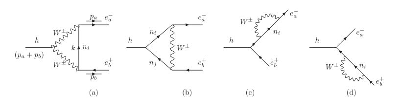
Figure 1: Feynman diagrams contributing to LFVHD in the unitary gauge.

The loop contributions are written as $\Delta_{L,R}=\Delta^{(a)}_{L,R}+\Delta^{(b)}_{L,R}+\Delta^{(c+d)}_{L,R}$, where the three terms come from private contributions of diagrams 1a), 1b), and sum of contributions from two diagrams c) and d), respectively. The analytic expressions of contributions from the three diagrams 1a), c), and d) can be derived directly from LFVHDUgauge , except the diagram 1b) containing the coupling $h\overline{n_{i}}n_{j}$. An analytic expression of $\Delta^{(b)}_{L,R}$ is derived in appendix C. We have used Form form to cross-check our results. In addition, the total $\Delta_{L,R}$ is consistent with the result calculated in the ’t Hooft Feynman gauge, as we will show later. Expressions of LFVHD contributions in the unitary gauge are

$$\Delta^{(a)}_{L} = -\frac{g^{3}m_{a}}{64\pi^{2}m_{W}^{3}}\sum_{i=1}^{K+3}U^{\nu*}_{ai}U^{\nu}_{bi}\left\{m_{n_{i}}^{2}\left(B^{(1)}_{1}-B^{(1)}_{0}-B^{(2)}_{0}\right)-m_{b}^{2}B^{(2)}_{1}+\left(2m_{W}^{2}+m^{2}_{h}\right)m_{n_{i}}^{2}C_{0}\right.$$

$$- \left.\left[2m_{W}^{2}\left(2m_{W}^{2}+m_{n_{i}}^{2}+m_{a}^{2}-m_{b}^{2}\right)+m_{n_{i}}^{2}m_{h}^{2}\right]C_{1}+\left[2m_{W}^{2}\left(m_{a}^{2}-m^{2}_{h}\right)+m_{b}^{2}m^{2}_{h}\right]C_{2}\frac{}{}\right\},$$

$$\Delta^{(a)}_{R} = -\frac{g^{3}m_{b}}{64\pi^{2}m_{W}^{3}}\sum_{i=1}^{K+3}U^{\nu*}_{ai}U^{\nu}_{bi}\left\{-m_{n_{i}}^{2}\left(B^{(2)}_{1}+B^{(1)}_{0}+B^{(2)}_{0}\right)+m_{a}^{2}B^{(1)}_{1}+\left(2m_{W}^{2}+m^{2}_{h}\right)m_{n_{i}}^{2}C_{0}\right.$$

$$- \left.\left[2m_{W}^{2}\left(m_{b}^{2}-m^{2}_{h}\right)+m_{a}^{2}m^{2}_{h}\right]C_{1}+\left[2m_{W}^{2}\left(2m_{W}^{2}+m_{n_{i}}^{2}-m_{a}^{2}+m_{b}^{2}\right)+m_{n_{i}}^{2}m_{h}^{2}\right]C_{2}\frac{}{}\right\},$$

$$\Delta^{(b)}_{L} = -\frac{g^{3}m_{a}}{64\pi^{2}m^{3}_{W}}\sum_{i,j=1}^{K+3}U^{\nu*}_{ai}U^{\nu}_{bj}\left\{C_{ij}\left[m^{2}_{n_{i}}B^{(1)}_{1}+m^{2}_{n_{j}}B^{(12)}_{0}-m^{2}_{n_{j}}m^{2}_{W}C_{0}\right.\right.$$

$$+ \left.\left.\left[2m^{2}_{n_{i}}m^{2}_{n_{j}}+2m_{W}^{2}\left(m^{2}_{n_{i}}+m^{2}_{n_{j}}\right)-(m^{2}_{n_{i}}m^{2}_{b}+m^{2}_{n_{j}}m^{2}_{a})\right]C_{1}\right]\right.$$

$$+ \left.C^{*}_{ij}m_{n_{i}}m_{n_{j}}\left[B^{(12)}_{0}+B^{(1)}_{1}-m_{W}^{2}C_{0}+\left(4m_{W}^{2}+m^{2}_{n_{i}}+m^{2}_{n_{j}}-m_{a}^{2}-m_{b}^{2}\right)C_{1}\right]\right\},$$

$$\Delta^{(b)}_{R} = -\frac{g^{3}m_{b}}{64\pi^{2}m^{3}_{W}}\sum_{i,j=1}^{K+3}U^{\nu*}_{ai}U^{\nu}_{bj}\left\{C_{ij}\left[-m^{2}_{n_{j}}B^{(2)}_{1}+m^{2}_{n_{i}}B^{(12)}_{0}-m^{2}_{n_{i}}m^{2}_{W}C_{0}\right.\right.$$ (14)

$$- \left.\left.\left[2m^{2}_{n_{i}}m^{2}_{n_{j}}+2m_{W}^{2}(m^{2}_{n_{i}}+m^{2}_{n_{j}})-(m^{2}_{n_{i}}m^{2}_{b}+m^{2}_{n_{j}}m^{2}_{a})\right]C_{2}\right]\right.$$

$$+ \left.C^{*}_{ij}m_{n_{i}}m_{n_{j}}\left[B^{(12)}_{0}-B^{(2)}_{1}-m_{W}^{2}C_{0}-\left(4m_{W}^{2}+m^{2}_{n_{i}}+m^{2}_{n_{j}}-m_{a}^{2}-m_{b}^{2}\right)C_{2}\right]\right\},$$

and

$$\Delta^{(c+d)}_{L} = \frac{g^{3}m_{a}}{64\pi^{2}m^{3}_{W}}\sum_{i=1}^{K+3}U^{\nu*}_{ai}U^{\nu}_{bi}\frac{m_{b}^{2}}{(m_{a}^{2}-m_{b}^{2})}\left[\left(2m_{W}^{2}+m_{n_{i}}^{2}\right)\left(B^{(1)}_{1}+B^{(2)}_{1}\right)\right.$$ (15)

$$+ \left.m_{a}^{2}B^{(1)}_{1}+m_{b}^{2}B^{(2)}_{1}-2m_{n_{i}}^{2}\left(B^{(1)}_{0}-B^{(2)}_{0}\right)\right],$$

$$\Delta^{(c+d)}_{R} = \frac{m_{a}}{m_{b}}\Delta^{(c+d)}_{L}.$$ (16)

Regarding $\Delta^{(b)}_{L,R}$, the contributions from $B^{(1)}_{1}=B^{(1)}_{1}(m_{W}^{2},m^{2}_{n_{i}})$ and $B^{(2)}_{1}$ are zeros because, for example, $B^{(1)}_{1}$ contains a factor $\sum_{j}U^{\nu}_{bj}m_{n_{j}}U^{\nu}_{cj}=\left(U^{\nu*}\hat{M}^{\nu}U^{\nu\dagger}\right)^{*}_{bc}=M^{\nu*}_{bc}=0$.

Divergence cancellation in the total amplitude is explained as follows. From divergent parts of the PV functions in Appendix A, the divergent parts of $\Delta^{(a)}_{L}$ and $\Delta^{(b)}_{L}$ are

$$\mathrm{Div}[\Delta^{(a)}_{L}] = -\frac{g^{3}m_{a}}{64\pi^{2}m^{3}_{W}}\sum_{i=1}^{K+3}U^{\nu*}_{ai}U^{\nu}_{bi}\left[m^{2}_{n_{i}}\left(\frac{-3}{2}\Delta_{\epsilon}\right)+m^{2}_{b}\frac{1}{2}\Delta_{\epsilon}\right]$$

$$= \frac{3g^{3}m_{a}}{128\pi^{2}m_{W}^{3}}\Delta_{\epsilon}\sum_{i=1}^{K+3}U^{\nu*}_{ai}U^{\nu}_{bi}m^{2}_{n_{i}},$$

$$\mathrm{Div}[\Delta^{(b)}_{L}] = -\frac{g^{3}m_{a}}{64\pi^{2}m^{3}_{W}}\left[\sum_{i,j=1}^{K+3}\sum_{c=1}^{3}U^{\nu*}_{ai}U^{\nu}_{ci}U^{\nu*}_{cj}U^{\nu}_{bj}\left(m^{2}_{n_{i}}\frac{1}{2}\Delta_{\epsilon}+m^{2}_{n_{j}}\Delta_{\epsilon}\right)\right.$$ (17)

$$+ \left.\sum_{i,j=1}^{K+3}\sum_{c=1}^{3}U^{\nu*}_{ai}U^{\nu*}_{ci}U^{\nu}_{cj}U^{\nu}_{bj}m_{n_{i}}m_{n_{j}}\Delta_{\epsilon}\right]$$

$$= \frac{g^{3}m_{a}}{128\pi^{2}m^{3}_{W}}\Delta_{\epsilon}\left[\sum_{i,j=1}^{K+3}\sum_{c=1}^{3}U^{\nu*}_{ai}U^{\nu}_{ci}U^{\nu*}_{cj}U^{\nu}_{bj}\left(m^{2}_{n_{i}}+2m^{2}_{n_{j}}\right)\right.$$

$$+ \left.\sum_{i,j=1}^{K+3}\sum_{c=1}^{3}U^{\nu*}_{ai}U^{\nu*}_{ci}U^{\nu}_{cj}U^{\nu}_{bj}2m_{n_{i}}m_{n_{j}}\right],$$

where the unitary property of $U^{\nu}$ is used to cancel the second term of $\mathrm{Div}[\Delta^{(a)}_{L}]$, namely $\sum_{i=1}^{K+3}U^{\nu*}_{ai}U^{\nu}_{bi}=\left(U^{\nu}U^{\nu\dagger}\right)_{ab}=0$. The second term of $\mathrm{Div}[\Delta^{(b)}_{L}]$ vanishes because $\sum_{i}U^{\nu*}_{ai}U^{\nu*}_{ci}m_{n_{i}}=\left(U^{\nu*}\hat{M}_{\nu}U^{\nu\dagger}\right)_{ac}=M^{\nu}_{ac}=0$ with all $a,c=1,2,3$. We simplify the first term of $\mathrm{Div}[\Delta^{(b)}_{L}]$ based on the following equalities

$$\sum_{i,j=1}^{K+3}\sum_{c=1}^{3}m^{2}_{n_{i}}U^{\nu*}_{ai}U^{\nu}_{ci}U^{\nu*}_{cj}U^{\nu}_{bj} = \sum_{i=1}^{K+3}\sum_{c=1}^{3}m^{2}_{n_{i}}U^{\nu*}_{ai}U^{\nu}_{ci}\sum_{j=1}^{K+3}U^{\nu*}_{cj}U^{\nu}_{bj}$$ (18)

$$= \sum_{i=1}^{K+3}\sum_{c=1}^{3}m^{2}_{n_{i}}U^{\nu*}_{ai}U^{\nu}_{ci}(U^{\nu}U^{\nu\dagger})_{bc}=\sum_{i=1}^{K+3}m^{2}_{n_{i}}U^{\nu*}_{ai}U^{\nu}_{bi}.$$

Similarly, we have $\sum_{i,j=1}^{K+3}\sum_{c=1}^{3}2m^{2}_{n_{j}}U^{\nu*}_{aj}U^{\nu}_{ci}U^{\nu*}_{cj}U^{\nu}_{bj}=\sum_{i=1}^{K+3}2m^{2}_{n_{i}}U^{\nu*}_{ai}U^{\nu}_{bi}$. Inserting these two results into $\mathrm{Div}[\Delta^{(b)}_{L}]$ will give $\mathrm{Div}[\Delta^{(b)}_{L}]+\mathrm{Div}[\Delta^{(a)}_{L}]=0$. With $\Delta^{(c+d)}_{L}$, the divergent parts of the two terms $m_{a}^{2}B^{(1)}_{1}$ and $m_{b}^{2}B^{(2)}_{1}$ vanish because of the GIM mechanism, while two sums $[B^{(1)}_{1}+B^{(2)}_{1}]$ and $[B^{(1)}_{0}-B^{(2)}_{0}]$ are finite. Hence, $\Delta_{L}$ is finite. $\Delta_{R}$ has the same conclusion.

III.2 Amplitude in the ’t Hooft Feynman gauge.

In the ’t Hooft Feynman gauge, there are ten form factors $F^{(i)}_{L,R}$, ($i=1,2,..,10$) corresponding to ten diagrams shown in Fig. 1 of Refs. EArganda ; iseesaw . The total contribution is $\Delta_{L,R}=\sum_{i=1}^{10}F^{i}_{L,R}$. Formulas of $F^{(i)}_{L,R}$ in terms of PV functions defined in LFVHDUgauge are as follows,

$$F^{(1)}_{L} = -\frac{g^{3}m_{a}}{64\pi^{2}m_{W}^{3}}\sum_{i,j=1}^{K+3}B_{ai}B^{*}_{bj}\left\{C_{ij}\left[m^{2}_{n_{j}}\left(B^{(12)}_{0}+m^{2}_{W}C_{0}\right)-\left(m_{a}^{2}m^{2}_{n_{j}}+m_{b}^{2}m^{2}_{n_{i}}-2m_{n_{i}}^{2}m^{2}_{n_{j}}\right)C_{1}\right]\right.$$

$$+ \left.m_{n_{i}}m_{n_{j}}C^{*}_{ij}\left[B^{(12)}_{0}+m^{2}_{W}C_{0}+\left(m^{2}_{n_{i}}+m^{2}_{n_{j}}-m^{2}_{a}-m^{2}_{b}\right)C_{1}\right]\right\},$$

$$F^{(1)}_{R} = -\frac{g^{3}m_{b}}{64\pi^{2}m_{W}^{3}}\sum_{i,j=1}^{K+3}B_{ai}B^{*}_{bj}\left\{C_{ij}\left[m^{2}_{n_{i}}\left(B^{(12)}_{0}+m^{2}_{W}C_{0}\right)+\left(m_{a}^{2}m^{2}_{n_{j}}+m_{b}^{2}m^{2}_{n_{i}}-2m_{n_{i}}^{2}m^{2}_{n_{j}}\right)C_{2}\right]\right.$$

$$+ \left.m_{n_{i}}m_{n_{j}}C^{*}_{ij}\left[B^{(12)}_{0}+m^{2}_{W}C_{0}-\left(m^{2}_{n_{i}}+m^{2}_{n_{j}}-m^{2}_{a}-m^{2}_{b}\right)C_{2}\right]\right\},$$

$$F^{(2)}_{L} = \frac{g^{3}m_{a}}{64\pi^{2}m_{W}^{3}}\sum_{i,j=1}^{K+3}B_{ai}B^{*}_{bj}\times 2m_{W}^{2}$$

$$\times \left\{C_{ij}\left[m^{2}_{n_{j}}C_{0}-\left(m^{2}_{n_{i}}+m^{2}_{n_{j}}\right)C_{1}\right]+m_{n_{i}}m_{n_{j}}C^{*}_{ij}\left(C_{0}-2C_{1}\right)\right\},$$

$$F^{(2)}_{R} = \frac{g^{3}m_{b}}{64\pi^{2}m_{W}^{3}}\sum_{i,j=1}^{K+3}B_{ai}B^{*}_{bj}\times 2m_{W}^{2}$$ (19)

$$\times \left\{C_{ij}\left[m^{2}_{n_{i}}C_{0}+\left(m^{2}_{n_{i}}+m^{2}_{n_{j}}\right)C_{2}\right]+m_{n_{i}}m_{n_{j}}C^{*}_{ij}\left(C_{0}+2C_{2}\right)\right\},$$

$$F^{(3)}_{L} = \frac{g^{3}m_{a}}{64\pi^{2}m_{W}^{3}}\sum_{i=1}^{K+3}B_{ai}B^{*}_{bi}\left[4m_{W}^{4}C_{1}\right],\hskip 14.22636ptF^{(3)}_{R}=\frac{g^{3}m_{b}}{64\pi^{2}m_{W}^{3}}\sum_{i=1}^{K+3}B_{ai}B^{*}_{bi}\left[-4m_{W}^{4}C_{2}\right],$$

$$F^{(4)}_{L} = -\frac{g^{3}m_{a}}{64\pi^{2}m_{W}^{3}}\sum_{i=1}^{K+3}B_{ai}B^{*}_{bi}\times m_{W}^{2}\left[-m_{n_{i}}^{2}C_{0}+\left(2m_{b}^{2}-m^{2}_{n_{i}}\right)C_{1}-m^{2}_{b}C_{2}\right],$$

$$F^{(4)}_{R} = -\frac{g^{3}m_{b}}{64\pi^{2}m_{W}^{3}}\sum_{i=1}^{K+3}B_{ai}B^{*}_{bi}m_{W}^{2}\left[B^{(12)}_{0}+3m^{2}_{n_{i}}C_{0}+\left(2m^{2}_{h}-2m^{2}_{b}-m^{2}_{a}\right)C_{1}+\left(m^{2}_{n_{i}}+2m^{2}_{b}\right)C_{2}\right],$$

$$F^{(5)}_{L} = -\frac{g^{3}m_{a}}{64\pi^{2}m_{W}^{3}}\sum_{i=1}^{K+3}B_{ai}B^{*}_{bi}m_{W}^{2}\left[B^{(12)}_{0}+3m^{2}_{n_{i}}C_{0}-\left(m^{2}_{n_{i}}+2m^{2}_{a}\right)C_{1}-\left(2m^{2}_{h}-m^{2}_{b}-2m^{2}_{a}\right)C_{2}\right],$$

$$F^{(5)}_{R} = -\frac{g^{3}m_{b}}{64\pi^{2}m_{W}^{3}}\sum_{i=1}^{K+3}B_{ai}B^{*}_{bi}m_{W}^{2}\left[-m_{n_{i}}^{2}C_{0}+m^{2}_{a}C_{1}-\left(2m_{a}^{2}-m^{2}_{n_{i}}\right)C_{2}\right],$$

$$F^{(6)}_{L} = -\frac{g^{3}m_{a}}{64\pi^{2}m^{3}_{W}}\sum_{i=1}^{K+3}B_{ai}B^{*}_{bi}\times m_{h}^{2}\left[m^{2}_{n_{i}}(C_{0}-C_{1})+m^{2}_{b}C_{2}\right],$$

$$F^{(6)}_{R} = -\frac{g^{3}m_{b}}{64\pi^{2}m^{3}_{W}}\sum_{i=1}^{K+3}B_{ai}B^{*}_{bi}\times m_{h}^{2}\left[m^{2}_{n_{i}}(C_{0}+C_{2})-m^{2}_{a}C_{1}\right],$$ (20)

$$F^{(7)}_{L} = \frac{g^{3}m_{a}}{64\pi^{2}m_{W}^{3}}\sum_{i=1}^{K+3}B_{ai}B^{*}_{bi}\frac{(D-2)m_{W}^{2}m_{b}^{2}}{(m_{a}^{2}-m_{b}^{2})}B^{(1)}_{1},\hskip 14.22636ptF^{(7)}_{R}=\frac{m_{a}}{m_{b}}F^{(7)}_{L},$$

$$F^{(9)}_{L} = \frac{g^{3}m_{a}}{64\pi^{2}m_{W}^{2}}\sum_{i=1}^{K+3}B_{ai}B^{*}_{bi}\frac{(D-2)m_{W}^{2}m^{2}_{b}}{(m_{a}^{2}-m_{b}^{2})}B^{(2)}_{1},\hskip 14.22636ptF^{(9)}_{R}=\frac{m_{a}}{m_{b}}F^{(9)}_{L},$$ (21)

$$F^{(8)}_{L} = -\frac{g^{3}m_{a}}{64\pi^{2}m^{3}_{W}}\sum_{i=1}^{K+3}B_{ai}B^{*}_{bi}\frac{m_{b}^{2}}{(m_{a}^{2}-m_{b}^{2})}\left[2m^{2}_{n_{i}}B^{(1)}_{0}-\left(m^{2}_{n_{i}}+m_{a}^{2}\right)B^{(1)}_{1}\right],$$

$$F^{(8)}_{R} = -\frac{g^{3}m_{b}}{64\pi^{2}m^{3}_{W}}\sum_{i=1}^{K+3}B_{ai}B^{*}_{bi}\frac{1}{(m_{a}^{2}-m_{b}^{2})}\left[m^{2}_{n_{i}}\left(m_{a}^{2}+m_{b}^{2}\right)B^{(1)}_{0}-m_{a}^{2}\left(m^{2}_{n_{i}}+m_{b}^{2}\right)B^{(1)}_{1}\right],$$

$$F^{(10)}_{L} = \frac{g^{3}m_{a}}{64\pi^{2}m^{3}_{W}}\sum_{i=1}^{K+3}B_{ai}B^{*}_{bi}\frac{1}{(m_{a}^{2}-m_{b}^{2})}\left[m^{2}_{n_{i}}\left(m_{a}^{2}+m_{b}^{2}\right)B^{(2)}_{0}+m_{b}^{2}\left(m^{2}_{n_{i}}+m_{a}^{2}\right)B^{(2)}_{1}\right],$$

$$F^{(10)}_{R} = \frac{g^{3}m_{b}}{64\pi^{2}m^{3}_{W}}\sum_{i=1}^{K+3}B_{ai}B^{*}_{bi}\frac{m^{2}_{a}}{(m_{a}^{2}-m_{b}^{2})}\left[2m^{2}_{n_{i}}B^{(2)}_{0}+\left(m^{2}_{n_{i}}+m_{b}^{2}\right)B^{(2)}_{1}\right],$$ (22)

where $B_{ai}=U^{\nu*}_{ai},B^{*}_{bj}=U^{\nu}_{bj}$, $C_{ij}=\sum_{c=1}^{3}U^{\nu}_{ci}U^{\nu*}_{cj}$, and $D=4-2\epsilon$ is the integral dimension defined in Appendix A. Although $F^{(7)}_{L,R}$ and $F^{(9)}_{L,R}$ contain $B$-functions, they are finite because of the GIM mechanism. Hence it can be replaced with $D=4$. Because $B^{(12)}_{0}=B^{(12)}_{0}(m_{W}^{2},m_{W}^{2})$ in $F^{(4)}_{R}$ and $F^{(5)}_{L}$ do not depend on $m_{n_{i}}$, therefore vanish because of the GIM mechanism. They will be ignored from now on.

Although our notations of PV functions are different from those in EArganda ; iseesaw , transformations between two sets of notations are, (see a detailed proving in Appendix B)

$$C_{0} \leftrightarrow C_{0},\hskip 14.22636ptC_{1}\leftrightarrow C_{12}-C_{11},\hskip 14.22636ptC_{2}\leftrightarrow C_{12},$$

$$B^{(12)}_{0} \leftrightarrow B_{0}(m^{2}_{W},m^{2}_{W}),\;B_{0}(m^{2}_{n_{i}},m^{2}_{n_{j}}),\quad B^{(1,2)}_{0}(M^{2}_{0},M^{2})\leftrightarrow B_{0}(m^{2}_{l_{k,m}},M^{2}_{0},M^{2}),$$

$$B^{(1)}_{1}(M^{2}_{0},M^{2}) \leftrightarrow -B_{1}(m^{2}_{l_{k}},M^{2}_{0},M^{2}),\hskip 14.22636ptB^{(2)}_{1}(M^{2}_{0},M^{2})\leftrightarrow B_{1}(m^{2}_{l_{m}},M^{2}_{0},M^{2}).$$ (23)

The PV functions used in our work were checked to be consistent with Looptools looptool , see details in KHHung . The differences between our results and those shown in iseesaw are minus signs in $F^{(4)}_{L,R}$ and $F^{(5)}_{L,R}$. Our formulas are consistent with the results presented in Ref. e1612.09290 , where the authors confirmed that these signs do not affect the results given in Ref. iseesaw .

Now we will check the consistence between total amplitudes calculated in two gauges. Regarding to triangle diagrams with two internal neutrino lines, the deviation of contributions in two gauge are determined as follows,

$$\delta_{1} = \Delta^{(b)}_{L}-\left(F^{(1)}_{L}+F^{(2)}_{L}\right)=-\frac{g^{3}}{4m_{W}^{3}}\frac{m_{a}}{16\pi^{2}}\sum_{i,j=1}^{K+3}B_{ai}B^{*}_{bj}C_{ij}m^{2}_{n_{i}}B^{(1)}_{1}(m^{2}_{W},m^{2}_{n_{i}})$$ (24)

$$= -\frac{g^{3}}{4m_{W}^{3}}\frac{m_{a}}{16\pi^{2}}\sum_{i=1}^{K+3}B_{ai}B^{*}_{bi}m^{2}_{n_{i}}\left(B^{(1)}_{0}(m^{2}_{n_{i}},m^{2}_{W})-B^{(1)}_{1}(m^{2}_{n_{i}},m^{2}_{W})\right),$$

where useful equalities of B-functions are used bardin . In addition, $C_{ij}$ in the first line of (24) is simplified using the same trick given in (18). Similarly, other deviations are

$$\delta_{2} = \Delta^{(a)}_{L}-\sum^{6}_{k=3}F^{(k)}_{L}=-\frac{g^{3}}{4m_{W}^{3}}\frac{m_{a}}{16\pi^{2}}\sum_{i=1}^{K+3}B_{ai}B^{*}_{bi}\left[-m_{b}^{2}B^{(2)}_{1}-m^{2}_{n_{i}}\left(B^{(1)}_{0}-B^{(1)}_{1}+B^{(2)}_{0}\right)\right],$$

$$\delta_{3} = \Delta^{(c+d)}_{L}-\sum^{10}_{k=7}F^{(k)}_{L}=-\frac{g^{3}}{4m_{W}^{3}}\frac{m_{a}}{16\pi^{2}}\sum_{i=1}^{K+3}B_{ai}B^{*}_{bi}\left[m_{b}^{2}B^{(2)}_{1}+m^{2}_{n_{i}}B^{(2)}_{0}\right],$$ (25)

where $B_{0,1,2}\equiv B_{0,1,2}(m^{2}_{n_{i}},m^{2}_{W})$. Then, it can be seen easily that $\delta_{1}+\delta_{2}+\delta_{3}=0$. Hence, the total amplitudes calculated in two gauges are the same.

IV LFVHD in the minimal and inverse seesaw models

IV.1 Parameterization the neutrino mixing matrix

To start, we consider a general expression of the neutrino mixing matrix $U^{\nu}$ numixing ,

$$U^{\nu}=\Omega\left(\begin{array}[]{cc}U&\mathbf{O}\\ \mathbf{O}&V\\ \end{array}\right),\hskip 14.22636pt$$ (26)

where $\mathbf{O}$ is a $3\times K$ null matrix, $U$ and $V$ are $3\times 3$ and $K\times K$ unitary matrices, respectively. The $\Omega$ is a $(K+3)\times(K+3)$ unitary matrix that can be formally written as

$$\Omega=\exp\left(\begin{array}[]{cc}\mathbf{O}&R\\ -R^{\dagger}&\mathbf{O}\\ \end{array}\right)=\left(\begin{array}[]{cc}1-\frac{1}{2}RR^{\dagger}&R\\ -R^{\dagger}&1-\frac{1}{2}R^{\dagger}R\\ \end{array}\right)+\mathcal{O}(R^{3}),$$ (27)

where $R$ is a $3\times K$ matrix where absolute values of al elements are smaller than unity. The unitary matrix $U=U_{\mathrm{PMNS}}$ is the Pontecorvo-Maki-Nakagawa-Sakata (PMNS) matrix upmns .

The mass matrices of neutrinos are written as follows,

$$\hat{M}_{N} = \mathrm{diag}(m_{n_{4}},\;m_{n_{5}},...,\;m_{n_{K+3}}),$$

$$m_{\nu} = U^{*}_{\mathrm{PMNS}}\mathrm{diag}(m_{n_{1}},\;m_{n_{2}},\;m_{n_{3}})U^{\dagger}_{\mathrm{PMNS}}=U^{*}_{\mathrm{PMNS}}\hat{m}_{\nu}U^{\dagger}_{\mathrm{PMNS}},$$ (28)

where $m_{n_{i}}$ is the physical masses of all neutrinos,

$$U_{\mathrm{PMNS}}=\left(\begin{array}[]{ccc}c_{12}c_{13}&s_{12}c_{13}&s_{13}e^{-i\delta}\\ -s_{12}c_{23}-c_{12}s_{23}s_{13}e^{i\delta}&c_{12}c_{23}-s_{12}s_{23}s_{13}e^{i\delta}&s_{23}c_{13}\\ s_{12}s_{23}-c_{12}c_{23}s_{13}e^{i\delta}&-c_{12}s_{23}-s_{12}c_{23}s_{13}e^{i\delta}&c_{23}c_{13}\\ \end{array}\right)\mathrm{diag}(1,\;e^{i\alpha},\;e^{i\beta}),$$ (32)

and $c_{ab}\equiv\cos\theta_{ab}$, $s_{ab}\equiv\sin\theta_{ab}$. In the normal hierarchy scheme, the best-fit values of neutrino oscillation parameters are given as actnuUpdate

$$\Delta m^{2}_{21} = 7.50\times 10^{-5}\;\mathrm{eV^{2}},\hskip 14.22636pt\Delta m^{2}_{31}=2.457\times 10^{-3}\;\mathrm{eV^{2}},$$

$$s^{2}_{12} = 0.304,\;s^{2}_{23}=0.452,\;s^{2}_{13}=0.0218,$$ (33)

where $\Delta m^{2}_{a1}=m^{2}_{n_{a}}-m^{2}_{n_{1}}$ ($a=2,3$). In this work, other parameters will be fixed as $\delta=\alpha=\beta=0$.

The condition of seesaw mechanism for neutrino mass generation is $|M_{D}|\ll|M_{N}|$, where $|M_{D}|$ and $|M_{N}|$ denote characteristic scales of $M_{D}$ and $M_{N}$, resulting in useful relations numixing ,

$$R^{*} \simeq M_{D}M_{N}^{-1},\hskip 14.22636ptm_{\nu}\simeq-M_{D}M_{N}^{-1}M^{T}_{D},$$

$$V^{*}\hat{M}_{N}V^{\dagger} \simeq M_{N}+\frac{1}{2}R^{T}R^{*}M_{N}+\frac{1}{2}M_{N}R^{\dagger}R.$$ (34)

Based on the second relation in (34), the matrix $M_{D}$ can be parameterized via a general $K\times 3$ matrix $\xi$, which satisfies the only condition $\xi^{T}\xi=I_{3}$ ibarra ; numixing ; EArganda , namely

$$M_{D}^{T}=iU_{N}^{*}\left(M^{d}_{N}\right)^{1/2}\xi\left(\hat{m}_{\nu}\right)^{1/2}U^{\dagger}_{\mathrm{PMNS}},$$ (35)

where $U_{N}$ is an unitary matrix diagonalizing $M_{N}$, $U_{N}^{T}M_{N}U_{N}=M^{d}_{N}=\mathrm{diag}(M_{1},M_{2},...,M_{K})$.

In the MSS mentioned in Apo ; EArganda , the particle content is different from the Standard Model (SM) by three additional right-handed neutrinos ($K=3$), $N_{R,I}\sim(1,1,0)$ with $I=1,2,3$. New notations of neutrino mass matrices are $m_{D}\equiv M_{D}$, and $m_{M}\equiv M_{N}$. They are the respective $3\times 3$ Dirac and Majorana mass matrices corresponding to the first and second term of (1), $(m_{D})_{iJ}=Y_{\nu,iJ}\langle\phi\rangle$, and $(m_{M})_{iJ}=m_{M,iJ}$. The matrix $m_{M}$ is real, symmetric and non-singular.

The mixing matrix in the ISS model considered in ref. iseesaw can be found approximately using the above general discussion with $K=6$. Relations of notations between two parameterizations in iseesaw and numixing are

$$M_{D}=(m_{D},\hskip 14.22636pt\mathcal{O}),\hskip 14.22636ptM_{N}=\left(\begin{array}[]{cc}\mathcal{O}&M_{R}\\ M^{T}_{R}&\mu_{X}\\ \end{array}\right),\hskip 14.22636ptm_{\nu}=M_{\mathrm{light}},$$ (38)

where $\mathcal{O}$ is the $3\times 3$ matrix with all elements being zeros. From the definition of the inverse matrix, $M^{-1}_{N}M_{N}=M_{N}M^{-1}_{N}=I_{6}$, we derive that

$$M^{-1}_{N}=\left(\begin{array}[]{cc}-M^{-1}&\left(M^{T}_{R}\right)^{-1}\\ M_{R}^{-1}&0\\ \end{array}\right),$$ (41)

where $M$ is defined as $M=M_{R}\mu_{X}^{-1}M_{R}^{T}$ iseesaw . From (34), we then find that numixing

$$R^{*}=M_{D}M_{N}^{-1} = \left(-m_{D}M^{-1},\hskip 14.22636ptm_{D}\left(M^{T}_{R}\right)^{-1}\right),$$

$$m_{\nu}=-M_{D}M_{N}^{-1}M_{D}^{T} = m_{D}\left(M_{R}^{T}\right)^{-1}\mu_{X}M_{R}^{-1}m_{D}^{T}=m_{D}M^{-1}m_{D}^{T}.$$ (42)

These two expressions are consistent with those given in iseesaw ; numixing , giving a parameterization of $m_{D}$ as follows,

$$m^{T}_{D}=U_{M}^{*}\mathrm{diag}(\sqrt{M_{1}},\;\sqrt{M_{2}},\;\sqrt{M_{3}})\xi^{\prime}\sqrt{\hat{m}_{\nu}}U^{\dagger}_{\mathrm{PMNS}},$$ (43)

where $U_{M}$ satisfies $M=U_{M}^{*}\mathrm{diag}(M_{1},\;M_{2},\;M_{3})U^{\dagger}_{M}$ and $\xi^{\prime}$ is a complex orthogonal matrix satisfying $\xi^{\prime}\xi^{\prime T}=I_{3}$. The mixing matrix $U^{\nu}$ now is a $9\times 9$ matrix.

In order to compare and mark relations between LFVHD in two MSS and ISS models, we will pay attention to only simply cases of choosing parameters. In the MSS model, the choice is $\xi=U_{N}=I_{3}$, leading to following simple expressions of Eqs. in (34), namely

$$M^{d}_{N}=M_{N},\quad R=-iU_{\mathrm{PMNS}}\,\hat{m}_{\nu}^{1/2}\left(M^{d}_{N}\right)^{-1/2},\hskip 14.22636ptV=I_{3},\quad\hat{M}_{N}=M^{d}_{N}+\hat{m}_{\nu}.$$ (44)

In the ISS model, from (43) we see that $m_{D}$ is parameterized in terms of many free parameters, hence it is enough to choose that $\mu_{X}=\mu_{X}I_{3}$. This parameter is a new scale making the most important difference between the neutrino mixing matrices in the ISS and MSS. We also assume that $M_{R}=\hat{M}_{R}=\mathrm{diag}(M_{R_{1}},\,M_{R_{2}},\,M_{R_{3}})$ and $\xi^{\prime}=I_{3}$. With $|\mu_{X}|\ll|M_{R}|$ we have

$$U_{M}=I_{3},\quad M^{d}_{N}=\left(\begin{matrix}\hat{M}_{R}&0\\ 0&\hat{M}_{R}\end{matrix}\right),\qquad V\simeq\dfrac{1}{\sqrt{2}}\left(\begin{matrix}-iI_{3}&I_{3}\\ iI_{3}&I_{3}\end{matrix}\right).$$ (45)

We can see that both $\hat{M}_{R}$ (ISS) and $M_{N}$ (MSS) play roles as exotic neutrino mass scales. Therefore, they are identified as neutrino masses in both models, $\hat{M}_{R}=M_{N}=\mathrm{diag}(m_{n_{4}},\,m_{n_{5}},\,m_{n_{6}})$. The differences between two models now are two mixing matrix $V$ in (45) and $R$, and the $\mu_{X}$ scale, which does not appear in the MSS model. The $\mu_{X}$ plays special roles in the ISS model via its appearance in the second sub-matrix of the mixing matrix $R$ given in (42). A simple relation between largest elements of $R$ matrices in two models is

$$R^{\mathrm{ISS}}\sim\sqrt{\frac{m_{n_{6}}}{\mu_{X}}}R^{\mathrm{MSS}},$$ (46)

where $m_{n_{6}}$ now is considered as exotic neutrino mass scale, $m_{n_{4}}\leq m_{n_{5}}\leq m_{n_{6}}$. The relation (46) is the main reason that explains why the Br of LFVHD predicted from the ISS is much larger than that from the MSS.

In the following, we will discuss on LFVHD in the MSS model. The results of LFVHD in the ISS model can be derived from discussion in the MSS model based on (46).

IV.2 Discussion on LFVHD

In the MSS model, our investigation will use three physical masses of exotic neutrinos, $m_{n_{4,5,6}}$, as free parameters. The matrix $M_{D}$ can be derived from relations (35), i.e $M_{D}=iU^{*}_{\mathrm{PMNS}}\left(M^{d}_{N}\,\hat{m}_{\nu}\right)^{1/2}$. As a result, the mixing matrix $U^{\nu}$ is written as a function of physical neutrino masses and $U_{\mathrm{PMNS}}$. To determine constrains of heavy neutrino masses $m_{n_{6}}$, we base on relations in (34), which suggest that $m_{n_{6}}\times m_{n_{3}}\simeq|M_{D}|^{2}<6\pi\times 174^{2}$, because of the perturbative limit of the Yukawa couplings $Y_{\nu,ij}$ iseesaw . Combing with the active neutrino data given in (33), where at least one active neutrino mass is not smaller than $\sqrt{\Delta m_{31}^{2}}=5\times 10^{-11}$ GeV, we get an upper constrain, $m_{n_{6}}<8\times 10^{15}$ GeV, when $m_{n_{1}}\ll\sqrt{\Delta m_{31}^{2}}$. The lower constrain is $m_{n_{6}}>|M_{D}|>m_{n_{3}}>5\times 10^{-11}$ GeV. Numerical illustrations are shown in Fig. 2, where three heavy neutrino masses are non-degenerate, $3m_{n_{4}}=2m_{n_{5}}=m_{n_{6}}$, and $m_{n_{1}}=10^{-12}\,\mathrm{GeV}\ll\sqrt{\Delta m_{31}^{2}}$.

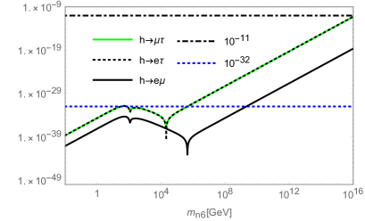
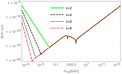
Figure 2: Left panel: Br$(h\rightarrow e_{a}e_{b})$ as functions of $m_{n_{6}}$ with non-degenerate heavy neutrino masses. Right panel: The dependence of Br$(h\rightarrow e_{a}e_{b})$ on the mixing matrix $U^{\nu}$ up to an order $\mathcal{O}(R^{k})$ with $k=2,4,6,8$.

The left panel of Fig. 2 presents Br$(h\rightarrow e_{a}e_{b})$ as functions of $m_{n_{6}}$. Unlike previous works such as Apo ; EArganda , heavy neutrinos masses were not considered at the interesting scale above $10^{10}$ GeV, where leptogenesis can be successful explained in the MSS frame work leptoMSS . More important, large values of heavy neutrinos may give large Br of LFVHD, as we have seen numerically. Unfortunately, values of $m_{n_{6}}\leq 8\times 10^{15}$ GeV gives an upper bound Br$(h\rightarrow\mu\tau)\leq\mathcal{O}(10^{-11})$. For other two decays, we get the relations Br$(h\rightarrow e\tau)\simeq$Br$(h\rightarrow\mu\tau)=(m^{2}_{\tau}/m^{2}_{\mu})$Br$(h\rightarrow e\mu)\simeq 287\times\mathrm{Br}(h\rightarrow e\mu)$. Hence, we just focus on the Br$(h\rightarrow\mu\tau)$.

The right panel of Fig. 2 shows values of Br$(h\rightarrow\mu\tau)$ in the whole valid range of $m_{n_{6}}$, namely $10^{-10}<m_{n_{6}}<8\times 10^{15}$ [GeV], where $U^{\nu}$ is considered up to $\mathcal{O}(R^{k})$. Each curve separates into three different parts. In the part with very heavy exotic neutrino masses, $m^{2}_{n_{6}}\gg m^{2}_{h},m^{2}_{W}$, i.e. $m_{n_{6}}>\mathcal{O}\left(10^{4}\right)$, we found a simple relation: Br$(h\rightarrow\mu\tau)=6.3\times 10^{-44}m_{n_{6}}^{2}\,[\mathrm{GeV}^{2}]$. On the other hand, for the part with very small exotic neutrino masses, $m^{2}_{n_{6}}\ll m^{2}_{\mu},m^{2}_{\tau}$, i.e. $m_{n_{6}}<\mathcal{O}\left(10^{-3}\right)$, there appears a new relation: Br$(h\rightarrow\mu\tau)=\dfrac{8.7\times 10^{-52}}{(m_{n_{6}}\mathrm{GeV})^{4}}$, when the matrix $\Omega$ is calculated up to $\mathcal{O}(R^{2})$. This will lead to the maximal values of Br$(h\rightarrow\mu\tau)\leq 10^{-11}$, the same order with large $m_{n_{6}}\sim\mathcal{O}(10^{15})$ GeV. If the matrix $\Omega$ is calculated more exactly, the Br$(h\rightarrow\mu\tau)$ will decrease significantly with small $m_{n_{6}}$, but will not change with large $m_{n_{6}}$. This can be explained from the conditions of the matrix $\Omega$, which is written in terms of the power series in $R$. If $m_{n_{6}}$ is small, $R\sim\sqrt{|m_{\nu}|/m_{n_{6}}}$ will be large as $m_{n_{6}}\rightarrow|M_{D}|\rightarrow|m_{\nu}|$. The calculation will be less accurate with smaller power $k$ included in $\Omega$. We consider more cases of $U^{\nu}$ where the matrix $\Omega$ in (27) is considered up to order $\mathcal{O}(R^{8})$. We conclude that the Br$(h\rightarrow\mu\tau)$ is very suppressed with small masses of exotic neutrinos. In contrast, large $m_{n_{6}}$ results in $|R|\ll 1$. Therefore, it is enough to consider the mixing matrix $U^{\nu}$ with order of $\mathcal{O}(R^{2})$ in the region where $m_{n_{6}}\geq 0.1$ GeV. In conclusion, to find large Br$(h\rightarrow\mu\tau)$, we just consider the region with large $m_{n_{6}}$.

To explain why large Br$(h\rightarrow\mu\tau)$ corresponds to large $m_{n_{6}}$, we pay attention to the properties of the mixing matrix $U^{\nu}$, the PV-functions and factors relating with them in the expressions of $\Delta^{(a)}_{L,R}$, $\Delta^{(b)}_{L,R}$, and $\Delta^{(c+d)}_{L,R}$. When $m^{2}_{n_{I}}\gg m^{2}_{h},m^{2}_{W}$, the terms with factors $m^{2}_{n_{I}}$ will give dominant contributions. The PV functions containing $m^{2}_{n_{I}}$ will have the following properties: $B_{0,1,2}(m^{2}_{n_{i}})=\mathcal{O}(10)$, $C_{0,1,2}(m^{2}_{n_{i}})\sim\ln(m^{2}_{n_{6}})/m^{2}_{n_{6}}$. Hence the largest contributions will come from $m^{2}_{n_{6}}B_{0,1,2}\sim m^{2}_{n_{6}}$ in $\Delta^{(a+c+d,b)}_{L,R}$ and $m^{4}_{n_{6}}C_{0,1,2}\sim[\ln\,m^{2}_{n_{6}}]m^{2}_{n_{6}}$ in $\Delta^{(b)}_{L,R}$.

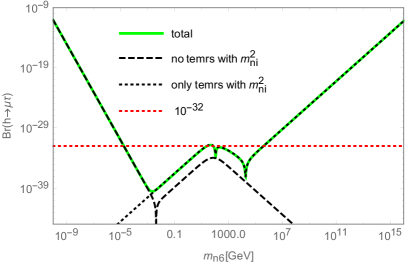
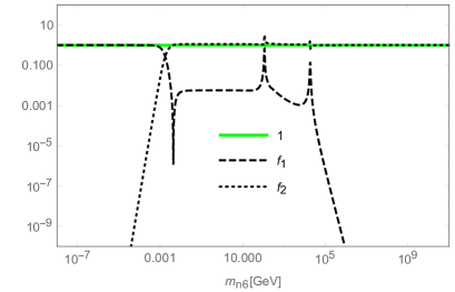
Figure 3: Comparing different contributions to Br$(h\rightarrow\mu\tau)$ as functions of heaviest exotic neutrino mass $m_{n_{6}}$, where $3m_{n_{4}}=2m_{n_{5}}=m_{n_{6}}$, $f_{1}=(\mathrm{no\;terms\;with\;m^{2}_{n_{i}})/total}$, and $f_{2}=\mathrm{(only\;terms\;with\;m^{2}_{n_{i}})/total}$.

The largest component of the matrix $R$ satisfies $R\sim\mathcal{O}\left(\sqrt{\frac{|\hat{m}_{\nu}|}{m_{n_{6}}}}\right)$. As a result, the mixing matrix elements in $\Delta^{(a+c+d)}_{L,R}$ and $\Delta^{(b)}_{L,R}$ will results in the following factors: $U^{\nu*}_{a(I+3)}U^{\nu}_{b(I+3)}=|R_{aI}|^{2}\sim\frac{|\hat{m}_{\nu}|}{m_{n_{6}}}$. There are new factors in the $\Delta^{(b)}_{L,R}$: $U^{\nu*}_{a(I+3)}U^{\nu}_{c(I+3)}U^{\nu*}_{c(J+3)}U^{\nu*}_{b(J+3)}\sim\frac{|\hat{m}_{\nu}|^{2}}{m^{2}_{n_{6}}}$. Hence the largest contribution to the total gives $\Delta_{L,R}\sim m_{n_{6}}$ with very large $m_{n_{6}}$, implying Br$(h\rightarrow\mu\tau)\sim m^{2}_{n_{6}}$. The correlations between terms with and without factors $m^{2}_{n_{i}}$ are shown in the Fig. 3. Terms without factors $m_{n_{i}}^{2}$ are dominant with tiny $m_{n_{6}}$ but they are very suppressed with large $m_{n_{6}}$.

The above discussions lead to new interesting results for LFVHD predicted by the MSS model, which were not concerned previously: i) the Br can reach values of order $10^{-11}$ with large values of heavy neutrino masses satisfying the perurbative limit; ii) the Br enhances with increasing $m_{n_{6}}$ above $10^{5}$ GeV. In addition, the maximal Br$(h\rightarrow\mu\tau)$ reaches the values of $10^{-33}-10^{-32}$ with $m_{n_{6}}\in[10^{2},10^{4}]$ GeV. We will show the relation between these interesting values and maximal values of Br$(h\rightarrow\mu\tau)$ predicted by the ISS.

We realize that the property of Br$(h\rightarrow\mu\tau)\sim m^{2}_{n_{6}}$ agrees very well with the approximate expression shown in Apo . In particular, Br$(h\rightarrow\mu\tau)\sim m^{4}_{n_{6}}\times|F_{N}|^{2}$, where $F_{N}\sim R^{2}\sim m^{-1}_{n_{6}}$ relating with active-heavy neutrino mixing elements in $U^{\nu}$. We believe that large values of the Br predicted in Apo arise from the reason that recent neutrino oscillation data could not be applied at that times. The numerical values of $F_{N}$ chosen in Apo may keep large contributions that should vanish because of the GIM mechanism.

Although the maximal Br of LFVHD predicted by the MSS is much smaller than the prediction from the ISS model given in EArganda ; iseesaw , the behave of the curve presenting Br$(h\rightarrow\mu\tau)$ shown in Fig. 3 have the same form with Br$(h\rightarrow\mu\tau)$ calculated in the ISS. The reason is as follows. If the exotic neutrino masses are fixed the same values in the two models, $m_{M}=M_{R}=\mathrm{diag}(m_{n_{4}},m_{n_{5}},m_{n_{6}})$, the important quantity making different contributions to LFVHD is the parametrization of $m_{D}$, see two Eqs. (35) and (43) for the MSS and ISS, respectively.

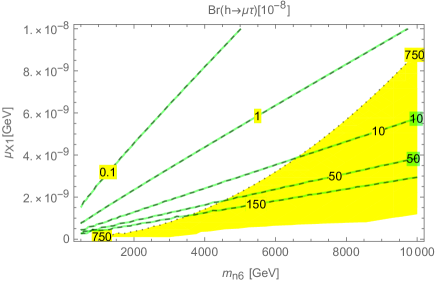
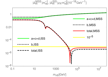
Figure 4: Left panel: contour plot of Br$(h\rightarrow\mu\tau)$ and $|m_{D}|$ as functions of $m_{n_{6}}$ and $\mu_{X}$, predicted from ISS framework. The yellow region is excluded by large $|m_{D}|>174\sqrt{6\pi}$ GeV. Dashed black curves are from ISS prediction. Green curves obtained from modifying MSS. The right panel: a comparison between different contributions from $|\Delta^{\mathrm{MSS}}_{R}|m^{-1}_{n_{6}}$ and $|\Delta^{\mathrm{ISS}}_{R}|\mu_{X}m^{-2}_{n_{6}}$.

This leads to the different structures of the $R$ matrices. The largest components of $R$ in the MSS are $R^{\mathrm{MSS}}_{aI}\sim\sqrt{\frac{|\hat{m}_{\nu}|}{|m_{n_{6}}|}}$ with $I>3$, while those in the ISS are $R^{\mathrm{ISS}}_{aI}\sim\sqrt{\frac{|\hat{m}_{\nu}|}{\mu_{X}}}$. Hence, in general the ISS mixing factors are larger than those of MSS a common factor $\sqrt{\frac{|\hat{m}_{n_{6}}|}{|\mu_{X}|}}$. It makes the prediction of Br of LFVHD by the ISS be much larger than the prediction by the MSS, provided large $m_{n_{6}}$ but small $\mu_{X}$. Unlike the MSS, where mass scale $m_{n_{6}}$ can be as large as $\mathcal{O}(10^{15})$ GeV, values of $m_{n_{6}}$ in the ISS are constrained by relation (42), i.e. $m^{2}_{n_{6}}|\hat{m}_{\nu}|/\mu_{X}=|m_{D}|^{2}<174^{2}\times 6\pi\,[\mathrm{GeV}]^{2}$. Hence, small $\mu_{X}$ will give small upper bounds of $m_{n_{6}}$, and large Br$(h\rightarrow\mu\tau)$ will depend complicatedly on these two parameters. The left panel of Fig. 4 shows possible values of Br$(h\rightarrow\mu\tau)$ in the allowed regions of $\mu_{{}_{X}}$ and $m_{n_{6}}$. Our numerical results are well consistent with previous work iseesaw . In addition, by adding a factor $\sqrt{\frac{|m_{n_{6}}|}{|\mu_{X}|}}$ into $R^{\mathrm{MSS}}$ and using the analytic expressions of $\Delta^{\mathrm{MSS}}_{L,R}$ we get a very consistent results of Br$(h\rightarrow\mu\tau)$ predicted by the ISS, see an illustration in the left panel of Fig. 4. This confirms again the consistence of our calculation for LFVHD in the MSS and ISS.

There is an interesting relation between two LFVHD amplitudes calculated in the two models, as drawn in the right panel of Fig. 4. Here, $|\Delta^{\mathrm{ISS}}_{R}|\mu_{X}m^{-2}_{n_{6}}$ and $|\Delta^{\mathrm{MSS}}_{R}|m^{-1}_{n_{6}}$ are considered as functions of $m_{n_{6}}$. We have checked numerically that $|\Delta^{\mathrm{ISS}}_{R}|\mu_{X}m^{-2}_{n_{6}}$ does not depend on $\mu_{X}$, and consistent with conclusion in iseesaw . It can be seen as follows. The dependence of $m_{D}$ and $R^{\mathrm{ISS}}$ on $M_{R}$ and $\mu_{X}$ can be separate into two parts. The first is the correlation between elements of these matrices in order to give correct experimental values of active neutrino data. And the second is the simple dependence on the scales of $m_{n_{6}}$ and $\mu_{X}$. In the ISS, $R^{\mathrm{ISS}}_{aI}=U^{\nu}_{a(I+3)}\sim\mu_{X}^{-1/2}$ and do not depend on $m_{n_{6}}$. Now, if we pay attention to the region with large $m_{n_{6}}$, the terms like $m_{n_{i}}^{2}B_{0,1,2}$ are dominant contributions to $\Delta_{L,R}$ because of the factors $m_{n_{i}}^{2}$. As a result, $\Delta^{(a+c+d)}_{L,R}$ containing a factor $U^{\nu*}_{ai}U^{\nu}_{bi}\sim\mu^{-1}_{X}$ will give an overall factor $\mu_{X}^{-1}m^{2}_{n_{6}}$. Hence $\Delta^{(a+c+d)}_{L,R}\mu_{X}m^{-2}_{n_{6}}$ may be constant, following the property of $B$-functions. On the other hand, $\Delta^{(b)}_{L,R}$ contains $U^{\nu*}_{ai}U^{\nu*}_{cj}U^{\nu}_{ci}U^{\nu}_{bj}\sim\mu^{-1}_{X}$ or $\mu^{-2}_{X}$, depending on both indices $i$ and $j$ or only one larger than 3. Because both $\Delta^{(a+c+d)}_{L,R}$ and $\Delta^{(b)}_{L,R}$ are still divergent, terms with $\mu^{-2}_{X}$ must vanish in order to guarantee a finite $\Delta_{L,R}$. This results in a common factor $\mu_{X}^{-1}m^{2}_{n_{6}}$ for $\Delta_{L,R}$. In the right panel of Fig. 4, values of $\mu_{X}m^{-2}_{n_{6}}\Delta^{(a+c+d)}_{L,R}$ and $\mu_{X}m^{-2}_{n_{6}}\Delta^{(b)}_{L,R}$ correspond to $\Delta_{\epsilon}=0$. But we checked numerically that $\mu_{X}^{-1}m^{2}_{n_{6}}\Delta_{L,R}$ is independent with $\Delta_{\epsilon}$. In addition, we can see that $\mu_{X}m^{-2}_{n_{6}}\Delta^{(a+c+d)}_{L,R}$ and $\mu_{X}m^{-2}_{n_{6}}\Delta^{(b)}_{L,R}$ always have opposite signs, which is consistent with the fact that divergences contained in them are really canceled. Two absolute contributions from $\Delta^{(a+c+d)}_{L,R}$ and $\Delta^{(b)}_{L,R}$ are the same order, and nearly degenerate with large $m_{n_{6}}$. They start canceling strongly each other from the electroweak range of $m_{n_{6}}$, giving a very small $\mu_{X}m^{-2}_{n_{6}}\Delta_{L,R}$. It is $10^{-5}$ times smaller than values of $\mu_{X}m^{-2}_{n_{6}}\Delta^{(b)}_{L,R}$.

The above discussion is the same for both models ISS and MSS, where $m^{-1}_{n_{6}}\Delta_{L,R}$ is the function considered in the MSS. The numerical results are also shown in the right panel of the Fig. 4. Consider a region $10\leq m_{n_{6}}\leq 10^{4}$ GeV, there is an equality that $m^{-1}_{n_{6}}\Delta^{\mathrm{MSS}}_{L,R}=\Delta^{\mathrm{ISS}}_{L,R}\mu_{X}m^{-2}_{n_{6}}$, implying $\mathrm{Br^{ISS}}(h\rightarrow\mu\tau)=\frac{m^{2}_{n_{6}}}{\mu^{2}_{X}}\mathrm{Br^{MSS}}(h\rightarrow\mu\tau)$. From previous discussion, where $\mathrm{Br^{MSS}}(h\rightarrow\mu\tau)\leq 10^{-32}$, we can derive the maximal $\mathrm{Br^{ISS}}(h\rightarrow\mu\tau)\leq 10^{-32}\times\mathcal{O}((10^{4}/10^{-9})^{2})=\mathcal{O}(10^{-6})$.

We can also estimate the maximal value of Br$(h\rightarrow\mu\tau)$ based on the numerical result shown in Fig. 4. If $m_{n_{6}}\geq 10^{5}$ GeV, we have $\Delta_{R}\simeq 10^{-24}\mu_{X}^{-1}m^{2}_{n_{6}}$, where small $\Delta_{L}$ is ignored. Equivalently, we have Br$(h\rightarrow\mu\tau)\simeq 10^{-45}\mu_{X}^{-2}m^{4}_{n_{6}}$. The condition of perturbative limit gives $m^{2}_{n_{6}}\times 5\times 10^{-11}/\mu_{X}=|m_{D}|^{2}\leq 174^{2}\times 6\pi$, leading to $\mu_{X}^{-2}m^{4}_{n_{6}}\leq\mathcal{O}(10^{36})$. Hence in the region of lagre $m_{n_{6}}\geq 10^{5}$ GeV, Br$(h\rightarrow\mu\tau)$ can reach maximal value of $\mathcal{O}(10^{-9})$. If $m_{n_{6}}<10^{5}$ GeV, the allowed region in the left panel of Fig. 4 shows that Br$(h\rightarrow\mu\tau)$ can reach values of $\mathcal{O}(10^{-7})$ only if $m_{n_{6}}$ is few TeV, $\mu_{X}$ is order of $10^{-9}$ GeV, and $m_{D}$ gets values very close to the perturbative limit.

V Conclusion

In this work, the LFVHD in the MSS and ISS models have been discussed where we have focused on new aspects that were not shown in previous works. We calculated the amplitude of the LFVHD using new analytical expressions of PV-functions discussed recently. From this we have checked the consistence of our results in many different ways: comparing them with results of previous works, calculating in two gauges of unitary and ’t Hooft-Feynman, checking analytically the divergent cancellation of the total amplitude. In the MSS framework, we investigated numerically the Br$(h\rightarrow\mu\tau)$ in the valid and large range of exotic neutrino mass scale, from $10^{-10}$ GeV to $10^{16}$ GeV. When applying the Casas-Ibarra parameterization to Yukwa couplings of heavy neutrinos, we found a new result that Br$(h\rightarrow\mu\tau)\sim m^{2}_{n_{6}}$ with large $m_{n_{6}}$, because the mixing matrix elements affecting mostly the LFVHD amplitude by factors of $m_{n_{6}}^{-1/2}$. But in the valid region of perturbative requiring $m_{n_{6}}<10^{16}$ GeV, the Br$(h\rightarrow\mu\tau)$ reaches maximal values of $\mathcal{O}(10^{-11})$, still far from the recent experimental consideration. Anyway, this may be a hint to improve the MSS to more relevant models predicting higher values of Br$(h\rightarrow\mu\tau)$, for example the ISS. In this model, the largest mixing factors contributing to LFVHD amplitude do not depend on the exotic neutrino mass scale $m_{n_{6}}$ but consist of a factor $\mu_{X}^{-1}$. Hence, if two models have the same neutrino mass scale, and the neutrino mixing matrices obey the Casas-Ibarra parameterization, there will be a very simple relation that $\mathrm{BR^{ISS}}(h\rightarrow\mu\tau)/\mathrm{BR^{MSS}}(h\rightarrow\mu\tau)\simeq m^{2}_{n_{6}}\mu^{-2}_{X}$. This explains why the signal of LFVHD in the ISS is extremely significant than that in MSS. But the perturbative condition does not allow both large $m_{n_{6}}$ and small $\mu_{X}$, which can predict large Br$(h\rightarrow\mu\tau)$. Hence, maximal Br$(h\rightarrow\mu\tau)$ is still $\mathcal{O}(10^{-7})$ with few TeV of heavy neutrino mass scale. Our discussion on LFVHD of the MSS suggests that Br$(h\rightarrow\mu\tau)$ may be large in the extended versions of the MSS which allow very large $m_{n_{6}}$. Finally, although we presented here a different way to calculate the LFVHD, our numerical results for the ISS are well consistent with those noted in previous works iseesaw ; e1612.09290 .

Appendix A One loop Passarino-Veltman functions

Calculation in this section relates with one-loop diagrams in the Fig. 1. The analytic expressions of the PV-functions are given in LFVHDUgauge and they were derived from the general forms given in Hooft , using only the conditions of very small masses of tau and muon. They are consistent with bardin . The denominators of the propagators are denoted as $D_{0}=k^{2}-M_{0}^{2}+i\delta$, $D_{1}=(k-p_{1})^{2}-M_{1}^{2}+i\delta$ and $D_{2}=(k+p_{2})^{2}-M_{2}^{2}+i\delta$, where $\delta$ is infinitesimally a positive real quantity. The scalar integrals are defined as

$$B^{(i)}_{0} \equiv \frac{\left(2\pi\mu\right)^{4-D}}{i\pi^{2}}\int\frac{d^{D}k}{D_{0}D_{i}},\quad B^{(12)}_{0}\equiv\frac{\left(2\pi\mu\right)^{4-D}}{i\pi^{2}}\int\frac{d^{D}k}{D_{1}D_{2}},$$

$$C_{0} \equiv C_{0}(M_{0},M_{1},M_{2})=\frac{1}{i\pi^{2}}\int\frac{d^{4}k}{D_{0}D_{1}D_{2}},$$

where $i=1,2$. In addition, $D=4-2\epsilon\leq 4$ is the dimension of the integral; $M_{0},~{}M_{1},~{}M_{2}$ are masses of virtual particles in the loop. The momenta satisfy conditions: $p^{2}_{1}=m^{2}_{1},~{}p^{2}_{2}=m^{2}_{2}$ and $(p_{1}+p_{2})^{2}=m^{2}_{h}$. In this work, $m_{h}$ is the SM-like Higgs mass, $m_{1,2}$ are lepton masses. The tensor integrals are

$$B^{\mu}(p_{i};M_{0},M_{i}) = \frac{\left(2\pi\mu\right)^{4-D}}{i\pi^{2}}\int\frac{d^{D}k\times k^{\mu}}{D_{0}D_{i}}\equiv B^{(i)}_{1}p^{\mu}_{i},$$

$$C^{\mu} = C^{\mu}(M_{0},M_{1},M_{2})=\frac{1}{i\pi^{2}}\int\frac{d^{4}k\times k^{\mu}}{D_{0}D_{1}D_{2}}\equiv C_{1}p_{1}^{\mu}+C_{2}p_{2}^{\mu}.$$

The PV functions are $B^{(i)}_{0,1}$, $B^{(12)}_{0}$ and $C_{0,1,2}$. The functions $C_{0,1,2}$ are finite while the remains are divergent. We define the common divergent part as $\Delta_{\epsilon}\equiv\frac{1}{\epsilon}+\ln 4\pi-\gamma_{E}+\ln\mu^{2}$ where $\gamma_{E}$ is the Euler constant. Then the divergent parts of the above scalar factors are $\mathrm{Div}[B^{(i)}_{0}]=\mathrm{Div}[B^{(12)}_{0}]=\Delta_{\epsilon}$, and $\mathrm{Div}[B^{(1)}_{1}]=-\mathrm{Div}[B^{(2)}_{1}]=\frac{1}{2}\Delta_{\epsilon}$.

For simplicity in calculation we use approximative forms of PV functions where $p_{1}^{2},p_{2}^{2}\rightarrow 0$. The function $C_{0}$ was given in LFVHDUgauge consistent with that discussed on bardin , namely

$$C_{0}=\frac{1}{m_{h}^{2}}\left[R_{0}(x_{0},x_{1})+R_{0}(x_{0},x_{2})-R_{0}(x_{0},x_{3})\right],$$

where $R_{0}(x_{0},x_{i})\equiv Li_{2}(\frac{x_{0}}{x_{0}-x_{i}})-Li_{2}(\frac{x_{0}-1}{x_{0}-x_{i}})$, $Li_{2}(z)$ is the di-logarithm function; $x_{1,2}$ are solutions of the equation $x^{2}-\left(\frac{m_{h}^{2}-M_{1}^{2}+M_{2}^{2}}{m_{h}^{2}}\right)x+\frac{M_{2}^{2}-i\delta}{m_{h}^{2}}=0$; $x_{0}=\frac{M_{2}^{2}-M_{0}^{2}}{m_{h}^{2}}$; and $x_{3}=\frac{-M_{0}^{2}+i\delta}{M_{1}^{2}-M_{0}^{2}}$.

Based on denner , the $B$-functions with small absolute values of external momenta can be written in stable forms in numerical computations. Defining $y_{ij}$ ($i,j=1,2$) are solutions of the equation $y^{2}p^{2}-y(p^{2}_{i}+M^{2}_{i}-M^{2}_{0})+M_{i}^{2}-i\delta=0$. New functions $f_{n}(y)$ are defined as follows,

$$f_{n}(y)\equiv(n+1)\int_{0}^{1}dt~{}t^{n}\ln\left(1-\frac{t}{y}\right),$$

so that they can be evaluated numerically stable way by choosing

$$f_{n}(x)=\left\{\begin{array}[]{cc}\left(1-y^{n+1}\right)\ln\frac{y-1}{y}-\sum_{l=0}^{n}\frac{y^{n-l}}{l+1}&\mathrm{if}~{}|y|<10,\\ \ln\left(1-\frac{1}{y}\right)+\sum_{l=n+1}^{\infty}\frac{y^{n-l}}{l+1}&\mathrm{if}~{}|y|\geq 10.\\ \end{array}\right.$$ (49)

The $B$-functions now can be expressed in terms of $f_{n}(y)$, namely

$$B_{0}^{(i)} = \Delta_{\epsilon}-\ln M_{i}^{2}-\sum_{j=1}^{2}f_{0}(y_{ij}),$$

$$B_{1}^{(i)} = (-1)^{i}\left[\frac{1}{2}\left(\Delta_{\epsilon}-\ln M_{i}^{2}\right)-\sum_{k=1}^{2}f_{0}(y_{ij})+\frac{1}{2}\sum_{k=1}^{2}f_{1}(y_{ij})\right].$$

Finally, the $B^{(12)}_{0}$ and $C_{1,2}$ functions are determined as follows,

$$B^{(12)}_{0} = \Delta_{\epsilon}-\ln M_{1}^{2}+2+\sum_{k=1}^{2}x_{k}\ln\left(1-\frac{1}{x_{k}}\right),$$

$$C_{1} = \frac{1}{m_{h}^{2}}\left[B^{(1)}_{0}-B_{0}^{(12)}+(M_{2}^{2}-M_{0}^{2})C_{0}\right],\;C_{2}=-\frac{1}{m_{h}^{2}}\left[B^{(2)}_{0}-B_{0}^{(12)}+(M_{1}^{2}-M_{0}^{2})C_{0}\right].$$

In our work above use the following notations, $m_{1}\equiv m_{a}$, $m_{2}\equiv m_{b}$, $p_{1}\equiv p_{a}$ and $p_{2}\equiv p_{b}$.

Appendix B Matching with notations in previous works

This section will show the equivalence given in (23). We recall notations used in EArganda ; iseesaw ; e1612.09290 as follows. The external momenta are $p^{\prime}_{1}$,$(-p_{2}^{\prime})$, and $p_{3}^{\prime}$ for ingoing Higgs boson, outgoing leptons $e_{a}$ and $e_{b}$,respectively. The prime is used to distinguish from the notions that were used in our work, especially those given in Sec. A. Three denominators of the propagators are $D^{\prime}_{0}=k^{2}-m_{1}^{2}$, $D^{\prime}_{1}=(k+p^{\prime}_{2})^{2}-m_{2}^{2}$ and $D^{\prime}_{2}=(k+p^{\prime}_{1}+p^{\prime}_{2})^{2}-m_{3}^{2}$. The one-lopp-three-point functions are defined as,

$$\int\frac{d^{4}k}{(2\pi)^{4}}\times\frac{\left\{1,k^{\mu}\right\}}{D^{\prime}_{0}D^{\prime}_{1}D^{\prime}_{2}} = \frac{i}{16\pi^{2}}\left\{C^{\prime}_{0},\,C^{\prime}_{\mu}=C_{11}p^{\prime}_{2\mu}+C_{12}p^{\prime}_{1\mu}\right\}.$$ (50)

The equivalence between above notations with those given in Sec. A are $p^{\prime}_{1}=p_{1}+p_{2}$, $p^{\prime}_{2}=-p_{1}$, $m_{1,2,3}=M_{0,1,2}$. As a result, we get $D^{\prime}_{0,1,2}=D_{0,1,2}$, leading to $C^{\prime}_{0}=C_{0}$ and $C^{\prime}_{\mu}=C_{\mu}$. But the scalar factors $C_{11,12}$ and $C_{1,2}$ are different, namely $C^{\prime}_{\mu}=C_{11}(-p_{1\mu})+C_{12}(p_{1\mu}+p_{2\mu})=(C_{12}-C_{11})p_{1\mu}+C_{12}p_{2\mu}$. Matching this with definition of $C_{\mu}$ defined in Sec. A. We obtain the equivalence for $C_{1,2}$ in (23). Other $B$-functions is proved easily so we omit here.

Appendix C Form factors in unitary gauge for LFVHD

The contribution from diagram in Fig. 1b) to the LFVHD amplitude is

$$i\mathcal{M}_{(b)} = \int\frac{d^{4}k}{(2\pi)^{4}}\times\bar{u}_{a}\left(\frac{ig}{\sqrt{2}}U^{\nu*}_{ai}\gamma^{\mu}P_{L}\right)\frac{i\left[(-k\!\!\!/+p_{a}\!\!\!\!\!/\,)+m_{n_{i}}\right]}{D_{1}}$$

$$\times \left[\frac{-ig}{2m_{W}}\sum_{c=1}^{3}C_{ij}\left(m_{n_{i}}P_{L}+m_{n_{j}}P_{R}\right)+C^{*}_{ij}\left(m_{n_{j}}P_{L}+m_{n_{i}}P_{R}\right)\right]$$

$$\times \frac{i\left[-(k\!\!\!/+p_{b}\!\!\!\!\!/\,)+m_{n_{j}}\right]}{D_{2}}\times\left(\frac{ig}{\sqrt{2}}U^{\nu}_{bj}\gamma^{\nu}P_{L}\right)v_{b}\times\frac{-i}{D_{0}}\times\left(g_{\mu\nu}-\frac{k_{\mu}k_{\nu}}{m^{2}_{W}}\right)$$

$$= \frac{-g^{3}}{4m_{W}}\sum_{i,j=1}^{K+3}\sum_{c=1}^{3}U^{\nu*}_{ai}U^{\nu}_{bj}\times\int\frac{d^{4}k}{(2\pi)^{4}}\frac{1}{D_{0}D_{1}D_{2}}\times\left(g_{\mu\nu}-\frac{k_{\mu}k_{\nu}}{m^{2}_{W}}\right)$$

$$\times \bar{u}_{a}\gamma^{\mu}P_{L}\left[(-k\!\!\!/+p\!\!/_{a})+m_{n_{i}}\right]\left[C_{ij}\left(m_{n_{i}}P_{L}+m_{n_{j}}P_{R}\right)\right.$$

$$+ \left.C^{*}_{ij}\left(m_{n_{j}}P_{L}+m_{n_{i}}P_{R}\right)\right]\left[-(k\!\!\!/+p\!\!/_{b})+m_{n_{j}}\right]\gamma^{\nu}P_{L}v_{b}.$$

The final result is

$$i\mathcal{M}_{(b)} = \frac{i}{16\pi^{2}}\times\frac{-g^{3}}{4m^{3}_{W}}\sum_{i,j=1}^{K+3}\sum_{c=1}^{3}U^{\nu*}_{ai}U^{\nu}_{bj}$$

$$\times \left\{m_{a}[\overline{u_{a}}P_{L}v_{b}]\left[C_{ij}\left(m^{2}_{n_{i}}B^{(1)}_{1}+m^{2}_{n_{j}}B^{(12)}_{0}+2\left[m^{2}_{n_{i}}m^{2}_{n_{j}}+m_{W}^{2}(m^{2}_{n_{i}}+m^{2}_{n_{j}})\right]C_{1}\right.\right.\right.$$

$$\left.\left.\left.-(m^{2}_{n_{i}}m^{2}_{b}+m^{2}_{n_{j}}m^{2}_{a})C_{1}-m^{2}_{n_{j}}m^{2}_{W}C_{0}\right)\right.\right.$$

$$+ \left.\left.C^{*}_{ij}m_{i}m_{j}\left(B^{(12)}_{0}+B^{(1)}_{1}-m_{W}^{2}C_{0}+\left[4m_{W}^{2}+m_{n_{i}}^{2}+m^{2}_{n_{j}}-m_{a}^{2}-m_{b}^{2}\right]C_{1}\right)\right]\right.$$

$$+ \left.m_{b}[\overline{u_{a}}P_{R}v_{b}]\left[C_{ij}\left(-m^{2}_{n_{j}}B^{(2)}_{1}+m^{2}_{n_{i}}B^{(12)}_{0}-2\left[m^{2}_{n_{i}}m^{2}_{n_{j}}+m_{W}^{2}(m^{2}_{n_{i}}+m^{2}_{n_{j}})\right]C_{2}\right.\right.\right.$$

$$\left.\left.\left.+(m^{2}_{n_{i}}m^{2}_{b}+m^{2}_{n_{j}}m^{2}_{a})C_{2}-m^{2}_{n_{i}}m^{2}_{W}C_{0}\right)\right.\right.$$

$$+ \left.\left.C^{*}_{ij}m_{i}m_{j}\left(B^{(12)}_{0}-B^{(2)}_{1}-m_{W}^{2}C_{0}-\left[4m_{W}^{2}+m_{n_{i}}^{2}+m^{2}_{n_{j}}-m_{a}^{2}-m_{b}^{2}\right]C_{2}\right)\right]\right\}.$$

References

- (1) The ATLAS Collaboration, Phys.Lett. B 716, 1 (2012); The CMS Collaboration, G. Aad et al, Phys. Lett. B 716, 30 (2012).
- (2) CMS Collaboration, Phys. Lett. B 749, 337 (2015); Phys.Lett. B763, 472 (2016); ATLAS Collaboration, JHEP 1511 (2015) 211; CMS Collaboration. 2015., CMS-PAS-HIG-14-040.
- (3) S. Kanemura, K. Matsuda, T. Ota, T. Shindou, E. Takasugi and K.Tsumura, Phys. Lett. B 599, 83 (2004); G. Blankenburg, J. Ellis and G. Isidori, Phys. Lett. B 712, 386 (2012); S. Davidson and P. Verdier, Phys. Rev. D 86, 111701 (2012); S. Bressler, A. Dery and A. Efrati, Phys. Rev. D 90, 015025 (2014); D. Aristizabal Sierra and A. Vicente, Phys. Rev. D 90, 115004 (2014); C. X. Yue, C. Pang and Y. C. Guo, J. Phys. G 42, 075003 (2015); S. Banerjee, B. Bhattacherjee, M. Mitra, M. Spannowsky, JHEP 1607 (2016) 059; I. Chakraborty, A. Datta, A. Kundu, J.Phys. G43 (2016) no.12, 125001.
- (4) A. Pilaftsis, Phys.Lett. B285 (1992) 68; J. G. Körner, A. Pilaftsis, K. Schilcher, Phys. Rev. D 47 (1993) 1080.
- (5) A. Pilaftsis, Z.Phys. C55 (1992) 275.
- (6) E. Arganda, A. M. Curiel, M. J. Herrero, D. Temes, Phys.Rev. D71 (2005) 035011.
- (7) E. Arganda, M. J. Herrero, X. Marcano and C. Weiland, Phys. Rev. D 91, 015001 (2015).
- (8) E. Arganda, M.J. Herrero, X. Marcano, R. Morales, A. Szynkman, Phys.Rev. D95, 095029 (2017), arxiv:1612.09290 [hep-ph].
- (9) A. Ilakovac, Phys.Rev. D62, 036010 (2000); J.L. Diaz-Cruz, J.J. Toscano, Phys.Rev. D 62, 116005 (2000); J. H. Garcia, N. Rius, A. Santamaria, JHEP 1611 (2016) 084; X. G. He, J. Tandean, Y. J. Zheng, JHEP 1509 (2015) 093.
- (10) W. Altmannshofer, S. Gori, A. L. Kagan, L. Silvestrini, J. Zupan, Phys. Rev. D 93 (2016), 031301; I. Doršner, S. Fajfer, A. Greljo, J. F. Kamenik, N. Košnik, Ivan Nišandžic, JHEP 1506 (2015) 108; R. Harnik, J. Kopp and J. Zupan, JHEP 1303, 026 (2013); A. Celis, V. Cirigliano and E. Passemar, Phys. Rev. D 89, 013008 (2014); A. Dery, A. Efrati, Y. Nir, Y. Soreq and V. Susi, Phys. Rev. D 90, 115022 (2014); J. Heeck, M. Holthausen, W. Rodejohann and Y. Shimizu, Nucl. Phys. B 896, 281 (2015); A. Crivellin, G. DAmbrosio and J. Heeck, Phys. Rev. D 91, 075006 (2015); L. D . Lima, C. S. Machado, R. D. Matheus, L. A. F. D. Prado, JHEP 1511, 074 (2015); I. d. M. Varzielas, O. Fischer, V. Maurer, JHEP 1508, 080 (2015); C. F. Chang, C. H. V. Chang, C. S. Nugroho, T. C. Yuan, Nucl.Phys. B910 (2016) 293; C. H. Chen, T. Nomura, Eur.Phys.J. C76 (2016) no.6, 353; K. Huitu, V. Keus, N. Koivunen, O. Lebedev, JHEP 1605 (2016) 026; K. Cheung, W. Y. Keung, P. Y. Tseng, Phys. Rev. D 93 (2016), 015010; A. Crivellin, G. D’Ambrosio, J. Heeck, Phys. Rev. Lett. 114 (2015) 151801; N. Bizot, S. Davidson, M. Frigerio, J. L. Kneur, JHEP 1603 (2016) 073; M. Sher, K. Thrasher, Phys. Rev. D 93, 055021 (2016); M. Aoki, S. Kanemura, K. Sakurai, H. Sugiyama, Phys.Lett. B763, 352 (2016); M. Lindner, M. Platscher, F.S. Queiroz, A Call for New Physics : The Muon Anomalous Magnetic Moment and Lepton Flavor Violation, arXiv:1610.06587 [hep-ph]; H.K. Guo, Y.Y. Li, T. Liu, M. R. Musolf, J. Shu, Lepton-Flavored Electroweak Baryogenesis, arXiv:1609.09849 [hep-ph]; P.S. Bhupal Dev, R. Franceschini, R.N. Mohapatra, Phys.Rev. D86 (2012) 093010; J. H. Garcia, T. Ohlsson, S. Riad, J. Wiren , JHEP 1704 (2017) 130 , arXiv:1701.05345 [hep-ph]; B. Yang, J. Han, N. Liu, Phys.Rev. D95 (2017) 035010; A. Lami, P. Roig, Phys.Rev. D94 (2016), 056001.
- (11) A. Brignole, A. Rossi, Phys. Lett. B 566, 217 (2003); A. Brignole, A. Rossi, Nucl. Phys. B 701, 53 (2004); M. Arana-Catania, E. Arganda, M. J. Herrero, JHEP 1309, 160 (2013); JHEP 1510, 192 (2015); E. Arganda, M. J. Herrero, X. Marcano, C. Weiland, Phys. Rev. D 93, 055010 (2016); P. T. Giang, L. T. Hue, D. T. Huong and H. N. Long, Nucl. Phys. B 864 (2012) 85; L. T. Hue, D. T. Huong, H .N. Long, H. T. Hung, N. H. Thao, Prog. Theor. Exp. Phys. 113B05 (2015); D. T. Binh, L. T. Hue, D. T. Huong, H. N. Long, Eur. Phys. J. C 74 (2014) 2851; E. Arganda, M. J. Herrero, R. Morales and A. Szynkman, JHEP 1603, 055 (2016); J. L. Diaz-Cruz, JHEP 0305, 036 (2003); S. Baek, Z.-F. Kang, JHEP 1603 (2016) 106; S. Baek, K. Nishiwaki , Phys. Rev. D 93 (2016), 015002; H.B. Zhang, T.F. Feng, S.M. Zhao, Y.L. Yan, Chin.Phys. C41 043106, (2017).
- (12) N. Bizot, S. Davidson, M. Frigerio, J. -L. Kneur, JHEP 1603 (2016) 073; F. J. Botella, G. C. Branco, M. Nebot, M. N. Rebelo, Eur. Phys. J. C 76 (2016), 161; S. Kanemura, T. Ota, T. Shindou and K. Tsumura, Phys. Rev. D 73, 016006 (2006); M. Arroyo, J. L. Diaz-Cruz, E. Diaz and J. A. Orduz-Ducuara; D. Das and A. Kundu, Phys. Rev. D 92, 015009 (2015).
- (13) L. T. Hue, H. N. Long, T. T. Thuc and T. Phong Nguyen, Nucl. Phys. B 907 (2016) 37; T.T. Thuc, L.T. Hue, H.N. Long, and T. Phong Nguyen, Phys.Rev. D93 (2016), 115026.
- (14) K.H. Phan, H.T. Hung, and L.T. Hue, Prog. Theor. Exp. Phys.2016, 113B03 (2016).
- (15) P. Minkowski, Phys. Lett. B 67, 421 (1977); M. Gell-Mann, P. Ramond and R. Slansky, in Supergravity proceedings, edited by P. Van Nieuwenhuizen and D. Z. Freedman (1979) [arXiv:1306.4669 [hep-th]]; T. Yanagida, in Proceedings of the Workshop on the Baryon Number of the Universe and Unified Theories, edited by O. Sawada and A. Sugamoto, (1979); R. N. Mohapatra and G. Senjanovic, Phys. Rev. Lett. 44 (1980) 912; J. Schechter and J. W. F. Valle, Phys. Rev. D 22 (1980) 2227.
- (16) R. N. Mohapatra, Phys. Rev. Lett. 56, 561 (1986); R. N. Mohapatra and J. W. F. Valle, Phys. Rev. D 34, 1642 (1986); J. Bernabeu, A. Santamaria, J. Vidal, A. Mendez and J. W. F. Valle, Phys. Lett. B 187, 303 (1987).
- (17) J.A. Casas, A. Ibarra, Nucl. Phys. B618,171 (2001).
- (18) A. Das, N. Okada, Phys.Rev. D88 (2013) 113001; A. Das, N. Okada, Bounds on heavy Majorana neutrinos in type-I seesaw and implications for collider searches, arXiv:1702.04668 [hep-ph]; M. Drewes, B. Garbrecht, D. Gueter, J. Klaric, JHEP 1612 (2016) 150 .
- (19) A. Ibarra, E. Molinaro, S.T. Petcov, JHEP 1009 (2010) 108; A. Das, P.S. B. Dev, N. Okada, Phys.Lett. B735 (2014) 364.
- (20) M. C. Gonzalez-Garcia, M. Maltoni, T. Schwetz, JHEP 1411 (2014) 052 .
- (21) H. K. Dreiner, H. E. Haber, S. P. Martin, Phys. Rept. 494, 1 (2010).
- (22) D. Y. Bardin, G. Passarino, ”The Standard Model in the making: Precision study of the electroweak interactions”, Clarendon Press-Oxford, 1999.
- (23) J. A. M. Vermaseren, ”New features of FORM”, arxiv: math-ph/0010025.
- (24) G. ’t Hooft and M. Veltman, Nucl. Phys. B 153, 365 (1979).
- (25) G. Belanger, F. Boudjema, J. Fujimoto, T. Ishikawa, T. Kaneko, K. Kato, Y. Shimizu, Phys.Rept. 430 (2006) 117; W. J. Marciano, C. Zhang, S. Willenbrock, Phys.Rev. D85 (2012) 013002; J. C. Romao, J.P. Silva, Int.J.Mod.Phys. A27 (2012) 1230025.
- (26) A. Denner and S. Dittmaier, Nucl.Phys. B734 (2006) 62, e-Print: hep-ph/0509141.
- (27) T. Hahn, M. Perez-Victoria, Comput. Phys. Commun. 118 (1999) 153 [hep-ph/9807565].
- (28) C. Patrignani et al. (Particle Data Group), Chinese Physics C, 40, 100001 (2016).
- (29) S. Davidson, and A. Ibarra, Phys.Lett. B535, 25 (2002); S. Pascoli (UCLA), S.T. Petcov, and C.E. Yaguna, Phys.Lett. B564, 241 (2003).
- (30) Z. Maki, M. Nakagawa and S. Sakata, Prog. Theor. Phys. 28 (1962) 870; B. Pontecorvo, Sov.Phys.JETP 7, 172 (1958), Zh.Eksp.Teor.Fiz. 34, 247 (1957) .