How to Escape Saddle Points Efficiently
Abstract
This paper shows that a perturbed form of gradient descent converges to a second-order stationary point in a number iterations which depends only poly-logarithmically on dimension (i.e., it is almost “dimension-free”). The convergence rate of this procedure matches the well-known convergence rate of gradient descent to first-order stationary points, up to log factors. When all saddle points are non-degenerate, all second-order stationary points are local minima, and our result thus shows that perturbed gradient descent can escape saddle points almost for free.
Our results can be directly applied to many machine learning applications, including deep learning. As a particular concrete example of such an application, we show that our results can be used directly to establish sharp global convergence rates for matrix factorization. Our results rely on a novel characterization of the geometry around saddle points, which may be of independent interest to the non-convex optimization community.
1 Introduction
Given a function , gradient descent aims to minimize the function via the following iteration:
where is a step size. Gradient descent and its variants (e.g., stochastic gradient) are widely used in machine learning applications due to their favorable computational properties. This is notably true in the deep learning setting, where gradients can be computed efficiently via back-propagation (Rumelhart et al., 1988).
Gradient descent is especially useful in high-dimensional settings because the number of iterations required to reach a point with small gradient is independent of the dimension (“dimension-free”). More precisely, for a function that is -gradient Lipschitz (see Definition 1), it is well known that gradient descent finds an -first-order stationary point (i.e., a point with ) within iterations (Nesterov, 1998), where is the initial point and is the optimal value of . This bound does not depend on the dimension of . In convex optimization, finding an -first-order stationary point is equivalent to finding an approximate global optimum.
In non-convex settings, however, convergence to first-order stationary points is not satisfactory. For non-convex functions, first-order stationary points can be global minima, local minima, saddle points or even local maxima. Finding a global minimum can be hard, but fortunately, for many non-convex problems, it is sufficient to find a local minimum. Indeed, a line of recent results show that, in many problems of interest, either all local minima are global minima (e.g., in tensor decomposition (Ge et al., 2015), dictionary learning (Sun et al., 2016a), phase retrieval (Sun et al., 2016b), matrix sensing (Bhojanapalli et al., 2016; Park et al., 2016), matrix completion (Ge et al., 2016), and certain classes of deep neural networks (Kawaguchi, 2016)). Moreover, there are suggestions that in more general deep newtorks most of the local minima are as good as global minima (Choromanska et al., 2014).
On the other hand, saddle points (and local maxima) can correspond to highly suboptimal solutions in many problems (see, e.g., Jain et al., 2015; Sun et al., 2016b). Furthermore, Dauphin et al. (2014) argue that saddle points are ubiquitous in high-dimensional, non-convex optimization problems, and are thus the main bottleneck in training neural networks. Standard analysis of gradient descent cannot distinguish between saddle points and local minima, leaving open the possibility that gradient descent may get stuck at saddle points, either asymptotically or for a sufficiently long time so as to make training times for arriving at a local minimum infeasible. Ge et al. (2015) showed that by adding noise at each step, gradient descent can escape all saddle points in a polynomial number of iterations, provided that the objective function satisfies the strict saddle property (see Assumption A2). Lee et al. (2016) proved that under similar conditions, gradient descent with random initialization avoids saddle points even without adding noise. However, this result does not bound the number of steps needed to reach a local minimum.
Though these results establish that gradient descent can find local minima in a polynomial number of iterations, they are still far from being efficient. For instance, the number of iterations required in Ge et al. (2015) is at least , where is the underlying dimension. This is significantly suboptimal compared to rates of convergence to first-order stationary points, where the iteration complexity is dimension-free. This motivates the following question: Can gradient descent escape saddle points and converge to local minima in a number of iterations that is (almost) dimension-free?
In order to answer this question formally, this paper investigates the complexity of finding -second-order stationary points. For -Hessian Lipschitz functions (see Definition 5), these points are defined as (Nesterov and Polyak, 2006):
Under the assumption that all saddle points are strict (i.e., for any saddle point , ), all second-order stationary points () are local minima. Therefore, convergence to second-order stationary points is equivalent to convergence to local minima.
This paper studies gradient descent with phasic perturbations (see Algorithm 1). For -smooth functions that are also Hessian Lipschitz, we show that perturbed gradient descent will converge to an -second-order stationary point in , where hides polylog factors. This guarantee is almost dimension free (up to factors), answering the above highlighted question affirmatively. Note that this rate is exactly the same as the well-known convergence rate of gradient descent to first-order stationary points (Nesterov, 1998), up to log factors. Furthermore, our analysis admits a maximal step size of up to , which is the same as that in analyses for first-order stationary points.
As many real learning problems present strong local geometric properties, similar to strong convexity in the global setting (see, e.g. Bhojanapalli et al., 2016; Sun and Luo, 2016; Zheng and Lafferty, 2016), it is important to note that our analysis naturally takes advantage of such local structure. We show that when local strong convexity is present, the -dependence goes from a polynomial rate, , to linear convergence, . As an example, we show that sharp global convergence rates can be obtained for matrix factorization as a direct consequence of our analysis.
1.1 Our Contributions
This paper presents the first sharp analysis that shows that (perturbed) gradient descent finds an approximate second-order stationary point in at most iterations, thus escaping all saddle points efficiently. Our main technical contributions are as follows:
-
•
For -gradient Lipschitz, -Hessian Lipschitz functions (possibly non-convex), gradient descent with appropriate perturbations finds an -second-order stationary point in iterations. This rate matches the well-known convergence rate of gradient descent to first-order stationary points up to log factors.
-
•
Under a strict-saddle condition (see Assumption A2), this convergence result directly applies for finding local minima. This means that gradient descent can escape all saddle points with only logarithmic overhead in runtime.
-
•
When the function has local structure, such as local strong convexity (see Assumption A3.a), the above results can be further improved to linear convergence. We give sharp rates that are comparable to previous problem-specific local analysis of gradient descent with smart initialization (see Section 1.2).
-
•
All the above results rely on a new characterization of the geometry around saddle points: points from where gradient descent gets stuck at a saddle point constitute a thin “band.” We develop novel techniques to bound the volume of this band. As a result, we can show that after a random perturbation the current point is very unlikely to be in the “band”; hence, efficient escape from the saddle point is possible (see Section 5).
1.2 Related Work
Over the past few years, there have been many problem-specific convergence results for non-convex optimization. One line of work requires a smart initialization algorithm to provide a coarse estimate lying inside a local neighborhood, from which popular local search algorithms enjoy fast local convergence (see, e.g., Netrapalli et al., 2013; Candes et al., 2015; Sun and Luo, 2016; Bhojanapalli et al., 2016). While there are not many results that show global convergence for non-convex problems, Jain et al. (2015) show that gradient descent yields global convergence rates for matrix square-root problems. Although these results give strong guarantees, the analyses are heavily tailored to specific problems, and it is unclear how to generalize them to a wider class of non-convex functions.
| Algorithm | Iterations | Oracle |
| Ge et al. (2015) | Gradient | |
| Levy (2016) | Gradient | |
| This Work | Gradient | |
| Agarwal et al. (2016) | Hessian-vector product | |
| Carmon et al. (2016) | Hessian-vector product | |
| Carmon and Duchi (2016) | Hessian-vector product | |
| Nesterov and Polyak (2006) | Hessian | |
| Curtis et al. (2014) | Hessian |
For general non-convex optimization, there are a few previous results on finding second-order stationary points. These results can be divided into the following three categories, where, for simplicity of presentation, we only highlight dependence on dimension and , assuming that all other problem parameters are constant from the point of view of iteration complexity:
Hessian-based: Traditionally, only second-order optimization methods were known to converge to second-order stationary points. These algorithms rely on computing the Hessian to distinguish between first- and second-order stationary points. Nesterov and Polyak (2006) designed a cubic regularization algorithm which converges to an -second-order stationary point in iterations. Trust region algorithms (Curtis et al., 2014) can also achieve the same performance if the parameters are chosen carefully. These algorithms typically require the computation of the inverse of the full Hessian per iteration, which can be very expensive.
Hessian-vector-product-based: A number of recent papers have explored the possibility of using only Hessian-vector products instead of full Hessian information in order to find second-order stationary points. These algorithms require a Hessian-vector product oracle: given a function , a point and a direction , the oracle returns . Agarwal et al. (2016) and Carmon et al. (2016) presented accelerated algorithms that can find an -second-order stationary point in steps. Also, Carmon and Duchi (2016) showed by running gradient descent as a subroutine to solve the subproblem of cubic regularization (which requires Hessian-vector product oracle), it is possible to find an -second-order stationary pointin iterations. In many applications such an oracle can be implemented efficiently, in roughly the same complexity as the gradient oracle. Also, when the function has a Hessian Lipschitz property such an oracle can be approximated by differentiating the gradients at two very close points (although this may suffer from numerical issues, thus is seldom used in practice).
Gradient-based: Another recent line of work shows that it is possible to converge to a second-order stationary point without any use of the Hessian. These methods feature simple computation per iteration (only involving gradient operations), and are closest to the algorithms used in practice. Ge et al. (2015) showed that stochastic gradient descent could converge to a second-order stationary point in iterations, with polynomial of order at least four. This was improved in Levy (2016) to using normalized gradient descent. The current paper improves on both results by showing that perturbed gradient descent can actually find an -second-order stationary point in steps, which matches the guarantee for converging to first-order stationary points up to polylog factors.
2 Preliminaries
In this section, we will first introduce our notation, and then present some definitions and existing results in optimization which will be used later.
2.1 Notation
We use bold upper-case letters to denote matrices and bold lower-case letters to denote vectors. means the entry of matrix . For vectors we use to denote the -norm, and for matrices we use and to denote spectral norm and Frobenius norm respectively. We use to denote the largest, the smallest and the -th largest singular values respectively, and for corresponding eigenvalues.
For a function , we use and to denote its gradient and Hessian, and to denote the global minimum of . We use notation to hide only absolute constants which do not depend on any problem parameter, and notation to hide only absolute constants and log factors. We let denote the d-dimensional ball centered at with radius ; when it is clear from context, we simply denote it as . We use to denote projection onto the set . Distance and projection are always defined in a Euclidean sense.
2.2 Gradient Descent
The theory of gradient descent often takes its point of departure to be the study of convex minimization where the function is both -smooth and -strongly convex:
Definition 1.
A differentiable function is -smooth (or -gradient Lipschitz) if:
Definition 2.
A twice-differentiable function is -strongly convex if
Such smoothness guarantees imply that the gradient can not change too rapidly, and strong convexity ensures that there is a unique stationary point (and hence a global minimum). Standard analysis using these two properties shows that gradient descent converges linearly to a global optimum (see e.g. (Bubeck et al., 2015)).
Theorem 1.
Assume is -smooth and -strongly convex. For any , if we run gradient descent with step size , iterate will be -close to in iterations:
In a more general setting, we no longer have convexity, let alone strong convexity. Though global optima are difficult to achieve in such a setting, it is possible to analyze convergence to first-order stationary points.
Definition 3.
For a differentiable function , we say that is a first-order stationary point if ; we also say is an -first-order stationary point if .
Under an -smoothness assumption, it is well known that by choosing the step size , gradient descent converges to first-order stationary points.
Theorem 2 ((Nesterov, 1998)).
Assume that the function is -smooth. Then, for any , if we run gradient descent with step size and termination condition , the output will be -first-order stationary point, and the algorithm will terminate within the following number of iterations:
Note that the iteration complexity does not depend explicitly on intrinsic dimension; in the literature this is referred to as “dimension-free optimization.”
A first-order stationary point can be either a local minimum or a saddle point or a local maximum. For minimization problems, saddle points and local maxima are undesirable, and we abuse nomenclature to call both of them “saddle points” in this paper. The formal definition is as follows:
Definition 4.
For a differentiable function , we say that is a local minimum if is a first-order stationary point, and there exists so that for any in the -neighborhood of , we have ; we also say is a saddle point if is a first-order stationary point but not a local minimum. For a twice-differentiable function , we further say a saddle point is strict (or non-degenerate) if .
For a twice-differentiable function , we know a saddle point must satify . Intuitively, for saddle point to be strict, we simply rule out the undetermined case , where Hessian information alone is not enough to check whether is a local minimum or saddle point. In most non-convex problems, saddle points are undesirable.
To escape from saddle points and find local minima in a general setting, we move both the assumptions and guarantees in Theorem 2 one order higher. In particular, we require the Hessian to be Lipschitz:
Definition 5.
A twice-differentiable function is -Hessian Lipschitz if:
That is, Hessian can not change dramatically in terms of spectral norm. We also generalize the definition of first-order stationary point to higher order:
Definition 6.
For a -Hessian Lipschitz function , we say that is a second-order stationary point if and ; we also say is -second-order stationary point if:
Second-order stationary points are very important in non-convex optimization because when all saddle points are strict, all second-order stationary points are exactly local minima.
Note that the literature sometime defines -second-order stationary point by two independent error terms; i.e., letting and . We instead follow the convention of Nesterov and Polyak (2006) by choosing to reflect the natural relations between the gradient and the Hessian. This definition of -second-order stationary point can also differ by reparametrization (and scaling), e.g. Nesterov and Polyak (2006) use . We choose our parametrization so that the first requirement of -second-order stationary point coincides with the requirement of -first-order stationary point, for a fair comparison of our result with Theorem 2.
3 Main Result
In this section we show that it possible to modify gradient descent in a simple way so that the resulting algorithm will provably converge quickly to a second-order stationary point.
The algorithm that we analyze is a perturbed form of gradient descent (see Algorithm 2). The algorithm is based on gradient descent with step size . When the norm of the current gradient is small () (which indicates that the current iterate is potentially near a saddle point), the algorithm adds a small random perturbation to the gradient. The perturbation is added at most only once every iterations.
To simplify the analysis we choose the perturbation to be uniformly sampled from a -dimensional ball666Note that uniform sampling from a -dimensional ball can be done efficiently by sampling where and (Harman and Lacko, 2010).. The use of the threshold ensures that the dynamics are mostly those of gradient descent. If the function value does not decrease enough (by ) after iterations, the algorithm outputs . The analysis in this section shows that under this protocol, the output is necessarily “close” to a second-order stationary point.
We first state the assumptions that we require.
Assumption A1.
Function is both -smooth and -Hessian Lipschitz.
The Hessian Lipschitz condition ensures that the function is well-behaved near a saddle point, and the small perturbation we add will suffice to allow the subsequent gradient updates to escape from the saddle point. More formally, we have:
Theorem 3.
Assume that satisfies A1. Then there exists an absolute constant such that, for any , , and constant , will output an -second-order stationary point, with probability , and terminate in the following number of iterations:
Strikingly, Theorem 3 shows that perturbed gradient descent finds a second-order stationary point in almost the same amount of time that gradient descent takes to find first-order stationary point. The step size is chosen as which is in accord with classical analyses of convergence to first-order stationary points. Though we state the theorem with a certain choice of parameters for simplicity of presentation, our result holds even if we vary the parameters up to constant factors.
Without loss of generality, we can focus on the case , as in Theorem 3. This is because in the case , standard gradient descent without perturbation—Theorem 2—easily solves the problem (since by A1, we always have , which means that all -second-order stationary points are -first order stationary points).
We believe that the dependence on at least one factor in the iteration complexity is unavoidable in the non-convex setting, as our result can be directly applied to the principal component analysis problem, for which the best known runtimes (for the power method or Lanczos method) incur a factor. Establishing this formally is still an open question however.
To provide some intuition for Theorem 3, consider an iterate which is not yet an -second-order stationary point. By definition, either (1) the gradient is large, or (2) the Hessian has a significant negative eigenvalue. Traditional analysis works in the first case. The crucial step in the proof of Theorem 3 involves handling the second case: when the gradient is small and the Hessian has a significant negative eigenvalue , then adding a perturbation, followed by standard gradient descent for steps, decreases the function value by at least , with high probability. The proof of this fact relies on a novel characterization of geometry around saddle points (see Section 5)
If we are able to make stronger assumptions on the objective function we are able to strengthen our main result. This further analysis is presented in the next section.
3.1 Functions with Strict Saddle Property
In many real applications, objective functions further admit the property that all saddle points are strict (Ge et al., 2015; Sun et al., 2016a, b; Bhojanapalli et al., 2016; Ge et al., 2016). In this case, all second-order stationary points are local minima and hence convergence to second-order stationary points (Theorem 3) is equivalent to convergence to local minima.
To state this result formally, we introduce a robust version of the strict saddle property (cf. Ge et al., 2015):
Assumption A2.
Function is -strict saddle. That is, for any , at least one of following holds:
-
•
.
-
•
.
-
•
is -close to — the set of local minima.
Intuitively, the strict saddle assumption states that the space can be divided into three regions: 1) a region where the gradient is large; 2) a region where the Hessian has a significant negative eigenvalue (around saddle point); and 3) the region close to a local minimum. With this assumption, we immediately have the following corollary:
Corollary 4.
Corollary 4 shows that by substituting in Theorem 3 using , the output of perturbed gradient descent will be in the -neighborhood of some local minimum.
Note although Corollary 4 only explicitly asserts that the output will lie within some fixed radius from a local minimum. In many real applications, we can further write as a function of gradient threshold , so that when decreases, decreases linearly or polynomially depending on . Meanwhile, parameter is always nondecreasing when decreases due to the nature of this strict saddle definition. Therefore, in these cases, the above corollary further gives a convergence rate to a local minimum.
3.2 Functions with Strong Local Structure
The convergence rate in Theorem 3 is polynomial in , which is similar to that of Theorem 2, but is worse than the rate of Theorem 1 because of the lack of strong convexity. Although global strong convexity does not hold in the non-convex setting that is our focus, in many machine learning problems the objective function may have a favorable local structure in the neighborhood of local minima (Ge et al., 2015; Sun et al., 2016a, b; Sun and Luo, 2016). Exploiting this property can lead to much faster convergence (linear convergence) to local minima. One such property that ensures such convergence is a local form of smoothness and strong convexity:
Assumption A3.a.
In a -neighborhood of the set of local minima , the function is -strongly convex, and -smooth.
Here we use different letter to denote the local smoothness parameter (in contrast to the global smoothness parameter ). Note that we always have . However, often even local -strong convexity does not hold. We thus introduce the following relaxation:
Assumption A3.b.
In a -neighborhood of the set of local minima , the function satisfies a -regularity condition if for any in this neighborhood:
| (1) |
Here is the projection on to the set . Note -regularity condition is more general and is directly implied by standard -smooth and -strongly convex conditions. This regularity condition commonly appears in low-rank problems such as matrix sensing and matrix completion, and has been used in Bhojanapalli et al. (2016); Zheng and Lafferty (2016), where local minima form a connected set, and where the Hessian is strictly positive only with respect to directions pointing outside the set of local minima.
Gradient descent naturally exploits local structure very well. In Algorithm 3, we first run Algorithm 2 to output a point within the neighborhood of a local minimum, and then perform standard gradient descent with step size . We can then prove the following theorem:
Theorem 5.
Theorem 5 says that if strong local structure is present, the convergence rate can be boosted to linear convergence (). In this theorem we see that sequence of iterations can be decomposed into two phases. In the first phase, perturbed gradient descent finds a -neighborhood by Corollary 4. In the second phase, standard gradient descent takes us from to -close to a local minimum. Standard gradient descent and Assumption A3.a (or A3.b) make sure that the iterate never steps out of a -neighborhood in this second phase, giving a result similar to Theorem 1 with linear convergence.
Finally, we note our choice of local conditions (Assumption A3.a and A3.b) are not special. The interested reader can refer to Karimi et al. (2016) for other relaxed and alternative notions of convexity, which can also be potentially combined with Assumptions to yield convergence results of a similar flavor as that of Theorem 5.
4 Example — Matrix Factorization
As a simple example to illustrate how to apply our general theorems to specific non-convex optimization problems, we consider a symmetric low-rank matrix factorization problem, based on the following objective function:
| (2) |
where . For simplicity, we assume , and denote , . Clearly, in this case the global minimum of function value is zero, which is achieved at where is the SVD of the symmetric real matrix .
The following two lemmas show that the objective function in Eq. (2) satisfies the geometric assumptions A1, A2,and A3.b. Moreover, all local minima are global minima.
Lemma 6.
For any , the function defined in Eq. (2) is -smooth and -Hessian Lipschitz, inside the region .
Lemma 7.
For function defined in Eq.(2), all local minima are global minima. The set of global minima is . Furthermore, satisfies:
-
1.
-strict saddle property.
-
2.
-regularity condition in neighborhood of .
One caveat is that since the objective function is actually a fourth-order polynomial with respect to , the smoothness and Hessian Lipschitz parameters from Lemma 6 naturally depend on . Fortunately, we can further show that gradient descent (even with perturbation) does not increase beyond . Then, applying Theorem 5 gives:
Theorem 8.
There exists an absolute constant such that the following holds. For the objective function in Eq. (2), for any and constant , and for , the output of , will be -close to the global minimum set , with probability , after the following number of iterations:
Theorem 8 establishes global convergence of perturbed gradient descent from an arbitrary initial point , including exact saddle points. Suppose we initialize at , then our iteration complexity becomes:
where is the condition number of the matrix . We see that in the second phase, when convergence occurs inside the local region, we require iterations which is the standard local linear rate for gradient descent. In the first phase, to find a neighborhood of the solution, our method requires a number of iterations scaling as . We suspect that this strong dependence on condition number arises from our generic assumption that the Hessian Lipschitz is uniformly upper bounded; it may well be the case that this dependence can be reduced in the special case of matrix factorization via a finer analysis of the geometric structure of the problem.
5 Proof Sketch for Theorem 3
In this section we will present the key ideas underlying the main result of this paper (Theorem 3). We will first argue the correctness of Theorem 3 given two important intermediate lemmas. Then we turn to the main lemma, which establishes that gradient descent can escape from saddle points quickly. We present full proofs of all these results in Appendix A. Throughout this section, we use and as defined in Algorithm 2.
5.1 Exploiting Large Gradient or Negative Curvature
Recall that an -second-order stationary point is a point with a small gradient, and where the Hessian does not have a significant negative eigenvalue. Suppose we are currently at an iterate that is not an -second-order stationary point; i.e., it does not satisfy the above properties. There are two possibilities:
-
1.
Gradient is large: , or
-
2.
Around saddle point: and .
The following two lemmas address these two cases respectively. They guarantee that perturbed gradient descent will decrease the function value in both scenarios.
Lemma 9 (Gradient).
Assume that satisfies A1. Then for gradient descent with stepsize , we have .
Lemma 10 (Saddle).
(informal) Assume that satisfies A1, If satisfies and , then adding one perturbation step followed by steps of gradient descent, we have with high probability.
We see that Algorithm 2 is designed so that Lemma 10 can be directly applied. According to these two lemmas, perturbed gradient descent will decrease the function value either in the case of a large gradient, or around strict saddle points. Computing the average decrease per step in function value yields the total iteration complexity. Since Algorithm 2 only terminate when the function value decreases too slowly, this guarantees that the output must be -second-order stationary point (see Appendix A for formal proofs).
5.2 Main Lemma: Escaping from Saddle Points Quickly
The proof of Lemma 9 is straightforward and follows from traditional analysis. The key technical contribution of this paper is the proof of Lemma 10, which gives a new characterization of the geometry around saddle points.
Consider a point that satisfies the the preconditions of Lemma 10 ( and ). After adding the perturbation (), we can view as coming from a uniform distribution over , which we call the perturbation ball. We can divide this perturbation ball into two disjoint regions: (1) an escaping region which consists of all the points whose function value decreases by at least after steps; (2) a stuck region . Our general proof strategy is to show that consists of a very small proportion of the volume of perturbation ball. After adding a perturbation to , point has a very small chance of falling in , and hence will escape from the saddle point efficiently.
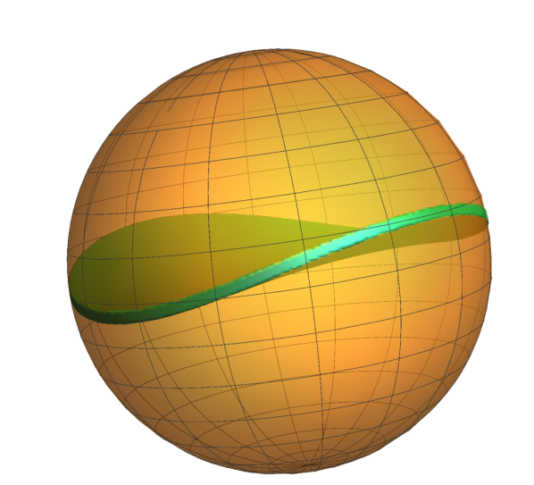
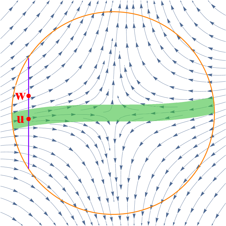
Let us consider the nature of . For simplicity, let us imagine that is an exact saddle point whose Hessian has only one negative eigenvalue, and positive eigenvalues. Let us denote the minimum eigenvalue direction as . In this case, if the Hessian remains constant (and we have a quadratic function), the stuck region consists of points such that has a small component. This is a straight band in two dimensions and a flat disk in high dimensions. However, when the Hessian is not constant, the shape of the stuck region is distorted. In two dimensions, it forms a “narrow band” as plotted in Figure 2 on top of the gradient flow. In three dimensions, it forms a “thin pancake” as shown in Figure 1.
The major challenge here is to bound the volume of this high-dimensional non-flat “pancake” shaped region . A crude approximation of this “pancake” by a flat “disk” loses polynomial factors in the dimensionalilty, which gives a suboptimal rate. Our proof relies on the following crucial observation: Although we do not know the explicit form of the stuck region, we know it must be very “thin,” therefore it cannot have a large volume. The informal statement of the lemma is as follows:
Lemma 11.
(informal) Suppose satisfies the precondition of Lemma 10, and let be the smallest eigendirection of . For any and any two points , if and , then at least one of is not in the stuck region .
Using this lemma it is not hard to bound the volume of the stuck region: we can draw a straight line along the direction which intersects the perturbation ball (shown as purple line segment in Figure 2). For any two points on this line segment that are at least away from each other (shown as red points in Figure 2), by Lemma 11, we know at least one of them must not be in . This implies if there is one point on this line segment, then on this line can be at most an interval of length around . This establishes the “thickness” of in the direction, which is turned into an upper bound on the volume of the stuck region by standard calculus.
6 Conclusion
This paper presents the first (nearly) dimension-free result for gradient descent in a general non-convex setting. We present a general convergence result and show how it can be further strengthened when combined with further structure such as strict saddle conditions and/or local regularity/convexity.
There are still many related open problems. First, in the presence of constraints, it is worthwhile to study whether gradient descent still admits similar sharp convergence results. Another important question is whether similar techniques can be applied to accelerated gradient descent. We hope that this result could serve as a first step towards a more general theory with strong, almost dimension free guarantees for non-convex optimization.
References
- Agarwal et al. [2016] Naman Agarwal, Zeyuan Allen-Zhu, Brian Bullins, Elad Hazan, and Tengyu Ma. Finding approximate local minima for nonconvex optimization in linear time. arXiv preprint arXiv:1611.01146, 2016.
- Bhojanapalli et al. [2016] Srinadh Bhojanapalli, Behnam Neyshabur, and Nathan Srebro. Global optimality of local search for low rank matrix recovery. arXiv preprint arXiv:1605.07221, 2016.
- Bubeck et al. [2015] Sébastien Bubeck et al. Convex optimization: Algorithms and complexity. Foundations and Trends® in Machine Learning, 8(3-4):231–357, 2015.
- Candes et al. [2015] Emmanuel J Candes, Xiaodong Li, and Mahdi Soltanolkotabi. Phase retrieval via wirtinger flow: Theory and algorithms. IEEE Transactions on Information Theory, 61(4):1985–2007, 2015.
- Carmon and Duchi [2016] Yair Carmon and John C Duchi. Gradient descent efficiently finds the cubic-regularized non-convex newton step. arXiv preprint arXiv:1612.00547, 2016.
- Carmon et al. [2016] Yair Carmon, John C Duchi, Oliver Hinder, and Aaron Sidford. Accelerated methods for non-convex optimization. arXiv preprint arXiv:1611.00756, 2016.
- Choromanska et al. [2014] Anna Choromanska, Mikael Henaff, Michael Mathieu, Gérard Ben Arous, and Yann LeCun. The loss surface of multilayer networks. arXiv:1412.0233, 2014.
- Curtis et al. [2014] Frank E Curtis, Daniel P Robinson, and Mohammadreza Samadi. A trust region algorithm with a worst-case iteration complexity of mathcal O( epsilon^-3/2) for nonconvex optimization. Mathematical Programming, pages 1–32, 2014.
- Dauphin et al. [2014] Yann N Dauphin, Razvan Pascanu, Caglar Gulcehre, Kyunghyun Cho, Surya Ganguli, and Yoshua Bengio. Identifying and attacking the saddle point problem in high-dimensional non-convex optimization. In Advances in Neural Information Processing Systems, pages 2933–2941, 2014.
- Ge et al. [2015] Rong Ge, Furong Huang, Chi Jin, and Yang Yuan. Escaping from saddle points—online stochastic gradient for tensor decomposition. In COLT, 2015.
- Ge et al. [2016] Rong Ge, Jason D Lee, and Tengyu Ma. Matrix completion has no spurious local minimum. In Advances in Neural Information Processing Systems, pages 2973–2981, 2016.
- Harman and Lacko [2010] Radoslav Harman and Vladimír Lacko. On decompositional algorithms for uniform sampling from n-spheres and n-balls. Journal of Multivariate Analysis, 101(10):2297–2304, 2010.
- Jain et al. [2015] Prateek Jain, Chi Jin, Sham M Kakade, and Praneeth Netrapalli. Computing matrix squareroot via non convex local search. arXiv preprint arXiv:1507.05854, 2015.
- Karimi et al. [2016] Hamed Karimi, Julie Nutini, and Mark Schmidt. Linear convergence of gradient and proximal-gradient methods under the Polyak-Lojasiewicz condition. In Joint European Conference on Machine Learning and Knowledge Discovery in Databases, pages 795–811. Springer, 2016.
- Kawaguchi [2016] Kenji Kawaguchi. Deep learning without poor local minima. In Advances In Neural Information Processing Systems, pages 586–594, 2016.
- Lee et al. [2016] Jason D Lee, Max Simchowitz, Michael I Jordan, and Benjamin Recht. Gradient descent only converges to minimizers. In Conference on Learning Theory, pages 1246–1257, 2016.
- Levy [2016] Kfir Y Levy. The power of normalization: Faster evasion of saddle points. arXiv preprint arXiv:1611.04831, 2016.
- Nesterov [1998] Yu Nesterov. Introductory lectures on convex programming volume i: Basic course. Lecture notes, 1998.
- Nesterov and Polyak [2006] Yurii Nesterov and Boris T Polyak. Cubic regularization of newton method and its global performance. Mathematical Programming, 108(1):177–205, 2006.
- Netrapalli et al. [2013] Praneeth Netrapalli, Prateek Jain, and Sujay Sanghavi. Phase retrieval using alternating minimization. In Advances in Neural Information Processing Systems, pages 2796–2804, 2013.
- Park et al. [2016] Dohyung Park, Anastasios Kyrillidis, Constantine Caramanis, and Sujay Sanghavi. Non-square matrix sensing without spurious local minima via the burer-monteiro approach. arXiv preprint arXiv:1609.03240, 2016.
- Polyak [1963] Boris T Polyak. Gradient methods for the minimisation of functionals. USSR Computational Mathematics and Mathematical Physics, 3(4):864–878, 1963.
- Rumelhart et al. [1988] David E Rumelhart, Geoffrey E Hinton, and Ronald J Williams. Learning representations by back-propagating errors. Cognitive modeling, 5, 1988.
- Sun et al. [2016a] Ju Sun, Qing Qu, and John Wright. Complete dictionary recovery over the sphere i: Overview and the geometric picture. IEEE Transactions on Information Theory, 2016a.
- Sun et al. [2016b] Ju Sun, Qing Qu, and John Wright. A geometric analysis of phase retrieval. In Information Theory (ISIT), 2016 IEEE International Symposium on, pages 2379–2383. IEEE, 2016b.
- Sun and Luo [2016] Ruoyu Sun and Zhi-Quan Luo. Guaranteed matrix completion via non-convex factorization. IEEE Transactions on Information Theory, 62(11):6535–6579, 2016.
- Zheng and Lafferty [2016] Qinqing Zheng and John Lafferty. Convergence analysis for rectangular matrix completion using burer-monteiro factorization and gradient descent. arXiv preprint arXiv:1605.07051, 2016.
Appendix A Detailed Proof of Main Theorem
In this section, we give detailed proof for the main theorem. We will first state two key lemmas that show how the algorithm can make progress when the gradient is large or near a saddle point, and show how the main theorem follows from the two lemmas. Then we will focus on the novel technique in this paper: how to analyze gradient descent near saddle point.
A.1 General Framework
In order to prove the main theorem, we need to show that the algorithm will not be stuck at any point that either has a large gradient or is near a saddle point. This idea is similar to previous works (e.g.[Ge et al., 2015]). We first state a standard Lemma that shows if the current gradient is large, then we make progress in function value.
Lemma 12 (Lemma 9 restated).
Assume satisfies A1, then for gradient descent with stepsize , we have:
Proof.
The next lemma says that if we are “close to a saddle points”, i.e., we are at a point where the gradient is small, but the Hessian has a reasonably large negative eigenvalue. This is the main difficulty in the analysis. We show a perturbation followed by small number of standard gradient descent steps can also make the function value decrease with high probability.
Lemma 13 (Lemma 10 formal).
The proof of this lemma is deferred to Section A.2. Using this Lemma, we can then prove the main Theorem.
Theorem 3.
There exist absolute constant such that: if satisfies A1, then for any , and constant , with probability , the output of will be second order stationary point, and terminate in iterations:
Proof.
Denote to be the absolute constant allowed in Theorem 13. In this theorem, we let , and choose any constant .
In this proof, we will actually achieve some point satisfying following condition:
| (3) |
Since , , we have , which implies any satisfy Eq.(3) is also a -second-order stationary point.
Starting from , we know if does not satisfy Eq.(3), there are only two possibilities:
- 1.
-
2.
: In this case, Algorithm 2 will add a perturbation of radius , and will perform gradient descent (without perturbations) for the next steps. Algorithm 2 will then check termination condition. If the condition is not met, we must have:
This means on average every step decreases the function value by
In case 1, we can repeat this argument for and in case 2, we can repeat this argument for . Hence, we can conclude as long as algorithm 2 has not terminated yet, on average, every step decrease function value by at least . However, we clearly can not decrease function value by more than , where is the function value of global minima. This means algorithm 2 must terminate within the following number of iterations:
Finally, we would like to ensure when Algorithm 2 terminates, the point it finds is actually an -second-order stationary point. The algorithm can only terminate when the gradient is small, and the function value does not decrease after a perturbation and iterations. We shall show every time when we add perturbation to iterate , if , then we will have . Thus, whenever the current point is not an -second-order stationary point, the algorithm cannot terminate.
According to Algorithm 2, we immediately know (otherwise we will not add perturbation at time ). By Lemma 13, we know this event happens with probability at least each time. On the other hand, during one entire run of Algorithm 2, the number of times we add perturbations is at most:
By union bound, for all these perturbations, with high probability Lemma 13 is satisfied. As a result Algorithm 2 works correctly. The probability of that is at least
Recall our choice of . Since , we have , this gives:
which finishes the proof.
∎
A.2 Main Lemma: Escaping from Saddle Points Quickly
Now we prove the main lemma (Lemma 13), which shows near a saddle point, a small perturbation followed by a small number of gradient descent steps will decrease the function value with high probability. This is the main step where we need new analysis, as the analysis previous works (e.g.[Ge et al., 2015]) do not work when the step size and perturbation do not depend polynomially in dimension .
Intuitively, after adding a perturbation, the current point of the algorithm comes from a uniform distribution over a -dimensional ball centered at , which we call perturbation ball. After a small number of gradient steps, some points in this ball (which we call the escaping region) will significantly decrease the function; other points (which we call the stuck region) does not see a significant decrease in function value. We hope to show that the escaping region constitutes at least fraction of the volume of the perturbation ball.
However, we do not know the exact form of the function near the saddle point, so the escaping region does not have a clean analytic description. Explicitly computing its volume can be very difficult. Our proof rely on a crucial observation: although we do not know the shape of the stuck region, we know the “width” of it must be small, therefore it cannot have a large volume. We will formalize this intuition later in Lemma 15.
The proof of the main lemma requires carefully balancing between different quantities including function value, gradient, parameter space and number of iterations. For clarify, we define following scalar quantities, which serve as the “units” for function value, gradient, parameter space, and time (iterations). We will use these notations throughout the proof.
Let the condition number be the ratio of the smoothness parameter (largest eigenvalue of Hessian) and the negative eigenvalue : , we define the following units:
Intuitively, if we plug in our choice of learning rate (which we will prove later) and hide the logarithmic dependences, we have , which is the only way to correctly discribe the units of function value, gradient, parameter space by just and . Moreover, these units are closely related, in particular, we know .
For simplicity of later proofs, we first restate Lemma 13 into a slightly more general form as follows. Lemma 13 is directly implied following lemma.
Lemma 14 (Lemma 13 restated).
There exists universal constant , for satisfies A1, for any , suppose we start with point satisfying following conditions:
Let where come from the uniform distribution over ball with radius , and let be the iterates of gradient descent from . Then, when stepsize , with at least probability , we have following for any :
Lemma 14 is almost the same as Lemma 13. It is easy to verify that by substituting and into Lemma 14, we immediately obtain Lemma 13.
Now we will formalize the intuition that the “width” of stuck region is small.
Lemma 15 (Lemma 11 restated).
There exists a universal constant , for any , let satisfies the conditions in Lemma 14, and without loss of generality let be the minimum eigenvector of . Consider two gradient descent sequences with initial points satisfying: (denote radius )
Then, for any stepsize , and any , we have:
Intuitively, lemma 15 claims for any two points inside the perturbation ball, if lies in the direction of minimum eigenvector of , and is greater than threshold , then at least one of two sequences will “efficiently escape saddle point”. In other words, if is a point in the stuck region, consider any point that is on a straight line along direction of . As long as is slightly far () from , it must be in the escaping region. This is what we mean by the “width” of the stuck region being small. Now we prove the main Lemma using this observation:
Proof of Lemma 14.
By adding perturbation, in worst case we increase function value by:
On the other hand, let radius . We know come froms uniform distribution over . Let denote the set of bad starting points so that if , then (thus stuck at a saddle point); otherwise if , we have .
By applying Lemma 15, we know for any , it is guaranteed that where . Denote be the indicator function of being inside set ; and vector , where is the component along direction, and is the remaining dimensional vector. Recall be -dimensional ball with radius ; By calculus, this gives an upper bound on the volumn of :
Then, we immediately have the ratio:
The second last inequality is by the property of Gamma function that as long as . Therefore, with at least probability , . In this case, we have:
which finishes the proof. ∎
A.3 Bounding the Width of Stuck Region
In order to prove Lemma 15, we do it in two steps:
-
1.
We first show if gradient descent from does not decrease function value, then all the iterates must lie within a small ball around (Lemma 16).
-
2.
If gradient descent starting from a point stuck in a small ball around a saddle point, then gradient descent from (moving along direction for at least a certain distance), will decreases the function value (Lemma 17).
Recall we assumed without loss of generality is the minimum eigenvector of . In this context, we denote , and for simplicity of calculation, we consider following quadratic approximation:
| (4) |
Now we are ready to state two lemmas formally:
Lemma 16.
For any constant , there exists absolute constant : for any , let satisfies the condition in Lemma 14, for any initial point with , define:
then, for any , we have for all that .
Lemma 17.
Note the conclusion in Lemma 17 equivalently means:
That is, for some , sequence “escape the saddle point” in the sense of sufficient function value decrease . Now, we are ready to prove Lemma 15.
Proof of Lemma 15.
W.L.O.G, let be the origin. Let be the absolute constant so that Lemma 17 holds, also let be the absolute constant to make Lemma 16 holds based on our current choice of . We choose so that our learning rate is small enough which make both Lemma 16 and Lemma 17 hold. Let and define:
Let’s consider following two cases:
Case :
Case :
A.3.1 Proof of Lemma 16
In Lemma 16, we hope to show if the function value did not decrease, then all the iterations must be constrained in a small ball. We do that by analyzing the dynamics of the iterations, and we decompose the -dimensional space into two subspaces: a subspace which is the span of significantly negative eigenvectors of the Hessian and its orthogonal compliment.
Recall notation and quadratic approximation as defined in Eq.(4). Since , we always have . W.L.O.G, set to be the origin, by gradient descent update function, we have:
| (5) |
Here, . By Hessian Lipschitz, we have , and by smoothness of the gradient, we have .
We will now compute the projections of in different eigenspaces of . Let be the subspace spanned by all eigenvectors of whose eigenvalue is less than . denotes the subspace of remaining eigenvectors. Let and denote the projections of onto and respectively i.e., , and . We can decompose the update equations Eq.(5) into:
| (6) | ||||
| (7) |
By definition of , we know for all :
Combined with the fact , we have:
where last inequality is due to . This gives:
| (8) |
Now, we use induction to prove that
| (9) |
Clearly Eq.(9) is true for since . Suppose Eq.(9) is true for all . We will now show that Eq.(9) holds for . Note that by the definition of , and , we only need to bound the last two terms of Eq.(8) i.e., and .
By update function of (Eq.(7)), we have:
| (10) |
and the norm of is bounded as follows:
| (11) |
The last step follows by choosing small enough constant and stepsize .
Bounding :
Bounding :
Using Eq.(10), we can also write the update equation as:
Combining with Eq.(11), this gives
Let the eigenvalues of to be , then for any , we know the eigenvalues of are . Let , and setting its derivative to zero, we obtain:
We see that is the unique maximizer, and is monotonically increasing in . This gives:
where . Therefore, we have:
| (13) |
The second last inequality is because by rearrange summation:
A.3.2 Proof of Lemma 17
In this Lemma we try to show if all the iterates from are constrained in a small ball, iterates from must be able to decrease the function value. In order to do that, we keep track of vector which is the difference between and . Similar as before, we also decompose into different eigenspaces. However, this time we only care about the projection of on the direction and its orthognal subspace.
Again, recall notation , as minimum eigenvector of and quadratic approximation as defined in Eq.(4). Since , we always have . W.L.O.G, set to be the origin. Define , by assumptions in Lemma 17, we have . Now, consider the update equation for :
where . By Hessian Lipschitz, we have . This gives the dynamic for satisfy:
| (14) |
Since , directly applying Lemma 16, we know for all . By condition of Lemma 17, we know for all . This gives:
| (15) |
This in sum gives for :
On the other hand, denote be the norm of projected onto direction, and be the norm of projected onto remaining subspace. Eq.(14) gives us:
where . We will now prove via induction that for all :
| (16) |
By hypothesis of Lemma 17, we know , thus the base case of induction holds. Assume Eq.(16) is true for , For , we have:
From above inequalities, we see that we only need to show:
By choosing , and , we have
This gives:
which finishes the induction.
Now, we know , this gives:
| (17) |
where the last step follows from .
Appendix B Improve Convergence by Local Structure
In this section, we show if the objective function has nice local structure (e.g. satisfies Assumptions A3.a or A3.b), then it is possible to combine our analysis with the local analysis in order to get very fast convergence to a local minimum.
In particular, we prove Theorem 5.
Theorem 5.
Proof.
Theorem 5 runs . According to algorithm 3, we know it calls first (denote its output as ), then run standard gradient descent with learning rate starting from .
By Corollary 4, we know is already in the -neighborhood of , where is the set of local minima. Therefore, to prove this theorem, we only need to show prove following two claims:
-
1.
Suppose is the sequence of gradient descent starting from with learning rate , then is always in the -neighborhood of .
- 2.
We will focus on Assumption A3.b (as we will later see Assumption A3.a is a special case of Assumption A3.b). Assume is in -neighborhood of , by gradient updates and the definition of projection, we have:
The second last inequality is due to -regularity condition. The last inequality is because of the choice .
There are two consequences of this calculation. First, it shows . As a result if in -neighborhood of , is also in this -neighborhood. Since is in the -neighborhood by Corollary 4, by induction we know all later iterations are in the same neighborhood.
Now, since we know all the points are in the neighborhood, the equation also shows linear convergence rate . The initial distance is bounded by , therefore to converge to points -close to , we only need the following number of iterations:
This finishes the proof under Assumption A3.b.
Finally, we argue assumption A3.a implies A3.b. First, notice that if a function is locally strongly convex, then its local minima are isolated: for any two points , the local region and must be disjoint (otherwise function is strongly convex in connected domain but has two distinct local minima, which is impossible). Therefore, W.L.O.G, it suffices to consider one perticular disjoint region, with unique local minimum we denote as , clearly, for all we have .
Appendix C Geometric Structures of Matrix Factorization Problem
In this Section we investigate the global geometric structures of the matrix factorization problem. These properties are summarized in Lemmas 6 and 7. Such structures allow us to apply our main Theorem and get fast convergence (as shown in Theorem 8).
Note that our main results Theorems 3 and 5 are proved for functions whose input is a vector. For the current function in 2, though the input is a matrix, we can always vectorize it to be a vector in and apply our results. However, for simplicity of presentation, we still write everything in matrix form (without explicit vectorization), while the reader should keep in mind the operations are same if one vectorizes everything first.
Recall for vectors we use to denote the 2-norm, and for matrices we use and to denote spectral norm, and Frobenius norm respectively. Furthermore, we always use to denote the -th largest singular value of the matrix.
We first show how the geometric properties (Lemma 6 and Lemma 7) imply a fast convergence (Theorem 8).
Theorem 8.
There exists an absolute constant such that the following holds. For matrix factorization (2), for any and constant , let , suppose we run , then:
-
1.
With probability 1, the iterates satisfy for every .
-
2.
With probability , the output will be -close to global minima set in following iterations:
Proof of Theorem 8.
Denote to be the absolute constant allowed in Theorem 5. In this theorem, we let , and choose any constant .
Theorem 8 consists of two parts. In part 1 we show that the iterations never bring the matrix to a very large norm, while in part 2 we apply our main Theorem to get fast convergence. We will first prove the bound on number of iterations assuming the bound on the norm. We will then proceed to prove part .
Part 2: Assume part of the theorem is true i.e., with probability , the iterates satisfy for every . In this case, although we are doing unconstrained optimization, we can still use the geometric properties that hold inside this region. .
By Lemma 6 and 7, we know objective function Eq.(2) is -smooth, -Lipschitz Hessian, -strict saddle, and holds -regularity condition in neighborhood of local minima (also global minima) . Furthermore, note and recall , then, we have:
Thus, we can choose . Substituting the corresponding parameters from Theorem 5, we know by running , with probability , the output will be -close to global minima set in iterations:
Part 1: We will now show part of the theorem. Recall PGDli (Algorithm 3) runs PGD (Algorithm 2) first, and then runs gradient descent within neighborhood of . It is easy to verify that neighborhood of is a subset of . Therefore, we only need to show that first phase PGD will not leave the region. Specifically, we now use induction to prove the following for PGD:
-
1.
Suppose at iteration we add perturbation, and denote to be the iterate before adding perturbation (i.e., , and ). Then, , and
-
2.
for all .
By choice of parameters of Algorithm 2, we know . First, consider gradient descent step without perturbations:
For the first term, we know function is monotonically increasing in . On the other hand, by induction assumption, we also know . Therefore, the max is taken when :
| (20) |
We seperate our discussion into following cases.
Case : In this case . Recall . Clearly, , we know:
This means that in each iteration, the spectral norm would decrease by at least .
Case : From (20), we know that as long as , we will always have . For , we have:
Thus, in this case, we always have .
In conclusion, if we don’t add perturbation in iteration , we have:
-
•
If , then .
-
•
If , then .
Now consider the iterations where we add perturbation. By the choice of radius of perturbation in Algorithm 2 , we increase spectral norm by at most :
The first inequality is because and . That is, if before perturbation we have , then .
On the other hand, according to Algorithm 2, once we add perturbation, we will not add perturbation for next iterations. Let :
This gives . Let be the next time when we add perturbation (), we immediately know for and .
Finally, by definition of , so the initial condition holds. This finishes induction and the proof of the theorem. ∎
In the next subsections we prove the geometric structures.
C.1 Smoothness and Hessian Lipschitz
Before we start proofs of lemmas, we first state some properties about gradient and Hessians. The gradient of the objective function is
Furthermore, we have the gradient and Hessian satisfy for any :
| (21) | ||||
| (22) |
Proof.
Denote , and recall .
Smoothness: For any , we have:
The last line is due to following decomposition and triangle inequality:
Hessian Lipschitz: For any , and any , according to Eq.(22), we have:
For term , we have:
For term , we have:
The inequality is due to following decomposition and triangle inequality:
Therefore, in sum we have:
∎
C.2 Strict-Saddle Property and Local Regularity
Recall the gradient and Hessian of objective function is calculated as in Eq.(21) and Eq.(22). We first prove an elementary inequality regarding to the trace of product of two symmetric PSD matrices. This lemma will be frequently used in the proof.
Lemma 18.
For both symmetric PSD matrices, we have:
Proof.
Let be the eigendecomposition of , where is diagonal matrix, and is orthogonal matrix. Then we have:
Since is PSD, we know is also PSD, thus the diagonal entries are non-negative. That is, for all . Finally, the lemma follows from the fact that and . ∎
Now, we are ready to prove Lemma 7.
Lemma 7.
For defined in Eq.(2), all local minima are global minima. The set of global minima is . Furthermore, satisfies:
-
1.
-strict saddle property, and
-
2.
-regularity condition in neighborhood of .
Proof.
Let us denote the set , in the end of proof, we will show this set is the set of all local minima (which is also global minima).
Throughout the proof of this lemma, we always focus on the first-order and second-order property for one matrix . For simplicity of calculation, when it is clear from the context, we denote and . By definition of , we know and , where
We first prove following claim, which will used in many places across this proof:
| (23) |
This because by expanding the Frobenius norm, and letting the SVD of be , we have:
Since are all orthonormal matrix, we know is also orthonormal matrix. Moreover for any orthonormal matrix , we have:
The last inequality is because is singular value thus non-negative, and is orthonormal, thus . This means the maximum of is achieved when , i.e., the minimum of is achieved when . Therefore, is symmetric PSD matrix.
Strict Saddle Property: In order to show the strict saddle property, we only need to show that for any satisfying and , we always have .
Let’s consider Hessian in the direction of . Clearly, we have:
and by (21):
Therefore, by Eq.(22) and above two equalities, we have:
Consider the first two terms, by expanding, we have:
where the second last inequality is because is the product of two symmetric PSD matrices (thus its trace is non-negative); the last inequality is by Lemma 18.
Finally, in case we have and
Local Regularity: In neigborhood of , by definition, we know,
Clearly, by Weyl’s inequality, we have , and . Moreover, since is symmetric matrix, we have:
At a highlevel, we will prove -regularity property (1) by proving that:
-
1.
, and
-
2.
.
According to (21), we know:
| (24) |
The last equality is because is symmetric matrix. Since is symmetric PSD matrix, and recall , by Lemma 18 we have:
| (25) |
On the other hand, we also have:
For term , by Lemma 18, and being a symmetric matrix, we have:
For term , by Eq.(23) we can denote which is symmetric PSD matrix, by Lemma 18, we have:
Combining with (24) we have:
| (26) |
Combining (25) and (26), we have:
∎