Density functional theory for dense nematics with steric interactions

Abstract

The celebrated work of Onsager on hard particle systems, based on the truncated second order virial expansion, is valid at relatively low volume fractions for large aspect ratio particles. While it predicts the isotropic-nematic phase transition, it does not provide a realistic equation of state in that the pressure remains finite for arbitrarily high densities. In this work, we derive a mean field density functional form of the Helmholtz free energy for nematics with hard core repulsion. In addition to predicting the isotropic-nematic transition, the model provides a more realistic equation of state. The energy landscape is much richer, and the orientational probability distribution function in the nematic phase possesses a unique feature—it vanishes on a nonzero measure set in orientation space.

I Introduction

An ensemble of non-spherical particles, interacting via hard core interactions, exhibits a first order isotropic-nematic phase transition as the number density increases, followed by a nematic-solid transition frenkel:phase ; Frenkel85 (see also the companion paper mulder:hard , for a number of technical results on the excluded volume of ellipsoids). In his celebrated theoretical work Onsager49 , Onsager successfully predicted the isotropic-nematic transition. Using the canonical ensemble, he expressed the free energy in terms of the orientational probability density function $f(\mathbf{\hat{l}})$, where $\mathbf{\hat{l}}\in\mathbb{S}^{2}$ is a unit vector along the symmetry axis of a particle. Truncating the virial expansion after the second term, in the low volume fraction limit, the free energy is of the form

$$F=NkT\left\{\ln\rho_{0}+\int_{\mathbb{S}^{2}}f(\mathbf{\hat{l}})\left(\ln f(\mathbf{\hat{l}})+\frac{1}{2}\rho_{0}\int_{\mathbb{S}^{2}}f(\mathbf{\hat{l}}^{\prime})V_{ex}(\mathbf{\hat{l}},\mathbf{\hat{l}}^{\prime})d\mathbf{\hat{l}}^{\prime}\right)d\mathbf{\hat{l}}\right\},$$ (1)

where $N$ is the number of particles, $k$ is Boltzmann’s constant, $T$ is the temperature and $\rho_{0}$ is the number density. In addition to the isotropic-nematic transition, the model describes phase separation and the coexistence of nematic and isotropic phases. In spite of its many successes mederos:hard , the theory has a major limitation: it does not provide a reasonable description of the behavior near the dense packing limit. It does not give a reasonable equation of state; the pressure remains finite at arbitrarily high number densities.

Onsager’s theory was rooted in the Mayer expansion, which formed the basis of Mayer’s statistical mechanics book mayer:statistical . Seen in the light of the full Mayer expansion (and the related problem of its convergence) the truncation at the first power in the number density in (1) appears unjustified. Many attempts have been made to explore the limits of validity of the Onsager theory and to propose extensions.

Straley straley:gas ; straley:third , by combining analytical and numerical methods, estimated the third virial coefficient for hard rods and concluded that Onsager’s theory would not be quantitatively accurate for values of the length-to-breadth ratio $\kappa$ less than $100$, a prediction that was far too pessimistic and that was indeed proven to be unrealistic by the Monte Carlo simulations of Frenkel and Mulder frenkel:phase ; Frenkel85 with ellipsoids of revolution. They showed that an ordering transition does take place already for ellipsoids of aspect ratio $\kappa=3$, though the densities involved could be too high to be compatible with the Onsager theory. It then became clear that it is not the degree of anisometry of the particles, but their density that may more easily challenge the validity of Onsager’s theory. The emphasis thus shifted from the particles’ shape to their filling fraction. A similar conclusion was drawn much later in the work of Tjipto-Margo and Evans tjipto-margo:onsager , who included the third virial coefficient in the theory for ellipsoids. For aspect ratios $\kappa>5$, their extended theory predicts the correct variation of the order parameter with density and is in agreement with simulations.

A valuable improvement to the Mayer paradigm of density expansion was introduced by Barboy and Gilbert barboy:series . They remarked that an expansion in the variable $y=\eta/(1-\eta)$, where $\eta$ denotes the volume fraction, has better convergence properties than the usual series in the number density. Their theory was applied to dumbbells and spherocylinders in the isotropic phase barboy:series , as well as to hard-parallelepipeds barboy:hard , but in the restricted-orientation approximation of Zwanzig zwanzig:first . No clear superiority of this theory to the classical Mayer theory was ever established with certainty mederos:hard .

A considerable step towards the extension of Mayer theory was taken by Parsons parsons:nematic and Lee lee:numerical , who moved along different lines of thought but arrived at one and the same theory. In Lee’s interpretation, the emphasis is on the equation of state, which is modelled after the theory of Carnahan and Starling carnahan:equation for real gases of hard spheres. The virial coefficients for the pressure expansion of Mayer’s theory are rescaled to those hypothesised by Carnahan and Starling in their extrapolation of the viral coefficients for hard spheres known at that time. As a consequence of this rescaling, the expansion for the free energy functional is re-summed exactly and expressed in the form of a modified Onsager bilinear functional in the probability distribution density. Lee applied this theory to a fluid of axially symmetric ellipsoids and found it in a better agreement with simulations than other theories available at that time lee:onsager . An alternative theory was independently proposed by Baus and co-workers baus:finite ; colot:density , which despite appearances is easily seen to reduce to the Parsons-Lee theory mederos:hard .

As successful as the Parsons-Lee theory may be, it is limited by being a re-summed version of the Mayer theory, and in so it remains exposed to all the unresolved issues concerned with the convergence of the underlying Mayer power series. We therefore attempt here to go beyond the Mayer paradigm.

In this paper, the density functional theory of aspherical hard particles is revisited. We are particularly interested in the phase behavior of hard ellipsoids at high densities, and near the densest packing limit. This very system will be used as a test case for the theory. Within the comfort zone of Mayer expansion, the evaluation of the partition function at high densities, even for hard spheres, has eluded researchers to date in spite of considerable effort. Here we take the simplest approach to explore orientational order in this regime. To clearly focus on this problem, we have chosen a minimal model, essentially at the van der Waals level. Although one might suspect that this form cannot provide quantitative predictions, our comparison with simulations for ellipsoids is encouraging. More generally, we feel that, in spite of its simplicity, it can give valuable insights into the consequences of the salient aspect of the problem: the depletion of available phase space as the density is increased.

A major challenge is the determination of the orientational distribution function subject to the hard constraint that the number of available states to the system is positive. This constraint is not always strictly enforced in the literature PPM . One striking result of this constraint, in the mean field limit, is that at densities above the isotropic-nematic transition, the orientational distribution function which minimizes the free energy has a compact support over orientation space. We also find that the nematic phase is more orientationally ordered than in the Onsager theory at the same density, and the density of the coexisting isotropic and nematic phases is a simple function of the particle shape. Our simple model gives a reasonable equation of state; that is, the pressure diverges at the dense packing limit.

The goal of the paper is to provide an approximate but near realistic description of dense orientationally ordered hard particle systems; currently available descriptions are either low density approximations Sheng75 ; Herzfeld , or they rely on somewhat ad hoc Carnahan-Starling type corrections to the free energy at high densities Jak1 ; Jak2 .

In Sec. II, we derive our theory. In Sec. III, we write the free energy for a system of hard ellipsoids with arbitrary number density, derive and solve the Euler-Lagrange equation for the probability density function, and arrive at the equation of state. In Sec. IV, we assume uniaxial nematic order, and present some numerical results relevant to this case. In Sec. IV.3, we discuss phase separation and two-phase coexistence. In Sec. V, we explore the possibility of biaxial equilibrium phases. Section VI is devoted to a close comparison with simulations. Finally, in Sec. VII we draw the conclusions of this study and summarize our results. The paper is closed by an Appendix, where we justify the approximate expression used in Sec. III for the excluded volume of ellipsoids of revolution.

II Theory

We consider a one-component system consisting of hard particles. For simplicity, we omit attractive interactions. The configurational Helmholtz free energy of a system of $N$ particles, within an additive constant, is

$$F=-kT\ln\frac{1}{N!}\int_{\Omega^{N}}e^{-\frac{1}{kT}\sum_{1\leq i<j\leq N}U_{ij}^{R}}d\mathbf{q}_{1}\cdots d\mathbf{q}_{N},$$ (2)

where $\mathbf{q}_{i}$ is the generalized (orientational and positional) coordinate of the $i^{th}$ particle, and $U_{ij}^{R}=U^{R}(\mathbf{q}_{i},\mathbf{q}_{j})$ is the repulsive interaction energy between particles $i$ and $j$, the sum is over all pairs of particles. Explicitly, the interaction potential is

$$U^{R}(\mathbf{q}_{i},\mathbf{q}_{j})=\begin{cases}\infty,&\text{if particles interpenetrate},\\ \ &\\ 0,&\text{otherwise}.\end{cases}$$ (3)

We write

$$G_{N}=\int_{\Omega^{N}}e^{-\frac{1}{kT}\Sigma_{1\leq i<j\leq N}U_{ij}^{R}}d\mathbf{q}_{1}\cdots d\mathbf{q}_{N},$$ (4)

where the quantity $G_{N}$ can be thought of as the number of states available to $N$ distinguishable particles. We consider adding one particle to the system. Then

$$G_{N+1}=\int_{\Omega^{N}}e^{-\frac{1}{kT}\Sigma_{1\leq i<j\leq N}U_{ij}^{R}}\left(\int_{\Omega}e^{-\frac{1}{kT}\Sigma_{i=1}^{N}U_{i(N+1)}^{R}}d\mathbf{q}_{N+1}\right)d\mathbf{q}_{1}\cdots d\mathbf{q}_{N},$$ (5)

and, since the probability density function of a given configuration is

$$P(\mathbf{q}_{1},\cdots,\mathbf{q}_{N})=\frac{e^{-\frac{1}{kT}\Sigma_{1\leq i<j\leq N}U_{ij}^{R}}}{G_{N}},$$ (6)

we have

$$G_{N+1} =G_{N}\int_{\Omega^{N}}P(\mathbf{q}_{1},\cdots,\mathbf{q}_{N})\left(\int_{\Omega}e^{-\frac{1}{kT}\Sigma_{i=1}^{N}U_{i(N+1)}^{R}}d\mathbf{q}_{N+1}\right)d\mathbf{q}_{1}\cdots d\mathbf{q}_{N}$$

$$=G_{N}\left\langle\int_{\Omega}e^{-\frac{1}{kT}\Sigma_{i=1}^{N}U_{i(N+1)}^{R}}d\mathbf{q}_{N+1}\right\rangle,$$ (7)

where the average is computed relative to $P$. Since all particles are equivalent, we may write

$$G_{N}=\left\langle\int_{\Omega}e^{-\frac{1}{kT}\Sigma_{i=2}^{N}U_{1i}^{R}}d\mathbf{q}_{1}\right\rangle^{N},$$ (8)

where the integral represents the average free volume per particle in an ensemble of $N$ particles. We can equivalently write this as

$$\begin{split}G_{N}&=\left\langle\int_{\Omega}1-(1-e^{-\frac{1}{kT}\Sigma_{i=2}^{N}U_{1i}^{R}})d\mathbf{q}_{1}\right\rangle^{N}\\ &=\left(\int_{\Omega}[1-W(\mathbf{q}_{1})]d\mathbf{q}_{1}\right)^{N},\end{split}$$ (9)

where

$$W(\mathbf{q}_{1})=\left\langle 1-e^{-\frac{1}{kT}\Sigma_{i=2}^{N}U_{1i}^{R}}\right\rangle$$ (10)

is the average excluded volume fraction.

The free energy then becomes

$$F=-kT\ln\frac{1}{N!}\left(\int_{\Omega}[1-W(\mathbf{q}_{1})]d\mathbf{q}_{1}\right)^{N}.$$ (11)

This important result is exact. The integrand in Eq. (11) can be regarded as the fraction of the total volume available to particle $1$, or the average free volume fraction. We next write that

$$W(\mathbf{q}_{1})=\frac{N}{V}v_{eff},$$ (12)

where $v_{eff}$ is the average volume effectively occupied by one particle. For two hard spheres of volume $v_{0}$, the pair excluded volume $V_{ex}$ is

$$V_{ex}=8v_{0},$$ (13)

and for $N=2$, Eq. (10) gives exactly

$$v_{eff}=\frac{1}{2}V_{ex}.$$ (14)

This is likely to remain a good approximation in the low density limit, as used in the Van der Waals equation (Israelachvili, , pp. 90–91), but it is clear from Eq. (10) as well as from experiments, that at high densities $v_{eff}$ is reduced considerably from this value. For close packed spheres, for example,

$$v_{eff}=\frac{3}{4\pi\sqrt{2}}V_{ex}\simeq\frac{1}{6}V_{ex}.$$ (15)

We write therefore that

$$v_{eff}=\lambda V_{ex},$$ (16)

where $\lambda$ is a parameter, taken to be nearly constant in our high density limit, to be determined by comparison with experiment. This justifies the following postulate of our theory:

$$W(\mathbf{q}_{1})=\lambda\int_{\Omega}\rho(\mathbf{q}_{2})\left(1-e^{-\frac{U^{R}(\mathbf{q}_{1},\mathbf{q}_{2})}{kT}}\right)d\mathbf{q}_{2},$$ (17)

where $\rho(\mathbf{q})$ is the number density of particles with generalized coordinate $\mathbf{q}$. More generally, in Eq. (17) $\lambda$ should be thought of as a function of the number density $\rho(\mathbf{q}_{1})$, for whose form we have yet to present a firm first-principles derivation. Here, $\lambda$ will be treated as an adjustable parameter; comparison with simulations will indicate the range within which the function $\lambda(\rho)$ is expected to vary.

To obtain the density functional form of the free energy, we assume that the density $\rho(\mathbf{q}_{i})$ is a slowly varying function of $\mathbf{q}_{i}$.  We consider an element $\Omega_{i}$ of phase space, containing $N_{i}$ particles and having volume $\Delta\mathbf{q}_{i}$, sufficiently small so that $\rho(\mathbf{q}_{i})$ in element $\Omega_{i}$ is nearly constant. The free energy $F_{i}$ of region $\Omega_{i}$ is of the form of Eq. (11); that is, by Stirling’s approximation,

$$F_{i}=-kT\ln\left(\frac{1}{N_{i}}\int_{\Omega_{i}}[1-W(\mathbf{q}_{i})]d\mathbf{q}_{i}\right)^{N_{i}},$$ (18)

and since $\rho(\mathbf{q}_{i})$ is nearly constant, we have that $N_{i}=\rho(\mathbf{q}_{i})\Delta\mathbf{q}_{i}$, and

$$F_{i}=-kT\ln\left(\frac{1}{\rho(\mathbf{q}_{i})}[1-W(\mathbf{q}_{i})]\right)^{\rho(\mathbf{q}_{i})\Delta\mathbf{q}_{i}}.$$ (19)

Then, since the free energy is additive, we can write for the entire system

$$F=-kT\ln{\prod}_{i}\left(\frac{1}{\rho(\mathbf{q}_{i})}[1-W(\mathbf{q}_{i})]\right)^{\rho(\mathbf{q}_{i})\Delta\mathbf{q}_{i}},$$ (20)

or, passing to the continuum limit,

$$F=kT\int_{\Omega}\rho(\mathbf{q})\ln\rho(\mathbf{q})d\mathbf{q}-kT\int_{\Omega}\rho(\mathbf{q})\ln[1-W(\mathbf{q})]d\mathbf{q},$$ (21)

which is the standard density functional form. Explicitly, this is

$$F=kT\int_{\Omega}\rho(\mathbf{q}_{1})\ln\rho(\mathbf{q}_{1})d\mathbf{q}_{1}-kT\int_{\Omega}\rho(\mathbf{q}_{1})\ln\left[1-\lambda\int_{\Omega}\rho(\mathbf{q}_{2})\left(1-e^{-\frac{U^{R}(\mathbf{q}_{1},\mathbf{q}_{2})}{kT}}\right)d\mathbf{q}_{2}\right]d\mathbf{q}_{1}.$$ (22)

For our problem, it is convenient to write the generalized coordinates in terms of position and orientation, then

$$\begin{split}F&=kT\int_{\mathbb{S}^{2}}\int_{\mathcal{B}}\rho(\mathbf{r}_{1},\mathbf{\hat{l}}_{1})\ln\rho(\mathbf{r}_{1},\mathbf{\hat{l}}_{1})d^{3}\mathbf{r}_{1}d^{2}\mathbf{\hat{l}}_{1}\\ &-kT\int_{\mathbb{S}^{2}}\int_{\mathcal{B}}\rho(\mathbf{r}_{1},\mathbf{\hat{l}}_{1})\ln\left[1-\lambda\int_{\mathbb{S}^{2}}\int_{\mathcal{B}}\rho(\mathbf{r}_{2},\mathbf{\hat{l}}_{2})\left(1-e^{-\frac{U^{R}(\mathbf{r}_{1},\mathbf{\hat{l}}_{1},\mathbf{r}_{2},\mathbf{\hat{l}}_{2})}{kT}}\right)d^{3}\mathbf{r}_{2}d^{2}\mathbf{\hat{l}}_{2}\right]d^{3}\mathbf{r}_{1}d^{2}\mathbf{\hat{l}}_{1},\end{split}$$ (23)

where $\rho(\mathbf{r},\mathbf{\hat{l}})$ is the number density of particles with center of mass at position $\mathbf{r}$, and orientation of symmetry axis along $\mathbf{\hat{l}}$. The unit sphere $\mathbb{S}^{2}$ is the orientation space. The region $\mathcal{B}$ in physical space denotes the position space, occupied by particles. In a homogeneous system, the density is independent of $\mathbf{r}$, so we write

$$\rho(\mathbf{r},\mathbf{\hat{l}})=\rho_{0}f(\mathbf{\hat{l}}),$$ (24)

where $\rho_{0}$ is now simply the number density of particles, and $f(\mathbf{\hat{l}})$ is the single particle orientational distribution function satisfying

$$\int_{\mathbb{S}^{2}}f(\mathbf{\hat{l}})d^{2}\mathbf{\hat{l}}=1.$$ (25)

Integrating over $\mathbf{r}_{2}$ in Eq. (23) gives

$$\int_{\mathbb{S}^{2}}\int_{\mathcal{B}}\rho_{0}f(\mathbf{\hat{l}}_{2})\left(1-e^{-\frac{U^{R}(\mathbf{r}_{1},\mathbf{\hat{l}}_{1},\mathbf{r}_{2},\mathbf{\hat{l}}_{2})}{kT}}\right)d^{3}\mathbf{r}_{2}d^{2}\mathbf{\hat{l}}_{2}=\rho_{0}\int_{\mathbb{S}^{2}}f(\mathbf{\hat{l}}_{2})V_{exc}(\mathbf{\hat{l}}_{1},\mathbf{\hat{l}}_{2})d^{2}\mathbf{\hat{l}}_{2},$$ (26)

where

$$V_{exc}(\mathbf{\hat{l}}_{1},\mathbf{\hat{l}}_{2})=\int_{\mathcal{B}}\left(1-e^{-\frac{U^{R}(\mathbf{r}_{1},\mathbf{\hat{l}}_{1},\mathbf{r}_{2},\mathbf{\hat{l}}_{2})}{kT}}\right)d^{3}\mathbf{r},$$ (27)

is the excluded volume of two particles, which depends only on the relative orientation of the particles with respect to one another. The free energy in Eq. (22) then becomes

$$F=kT\rho_{0}V\left[\ln\rho_{0}+\int_{\mathbb{S}^{2}}f(\mathbf{\hat{l}}_{1})\ln f(\mathbf{\hat{l}}_{1})d^{2}\mathbf{\hat{l}}_{1}-\int_{\mathbb{S}^{2}}f(\mathbf{\hat{l}}_{1})\ln\left(1-\lambda\rho_{0}\int_{\mathbb{S}^{2}}f(\mathbf{\hat{l}}_{2})V_{exc}(\mathbf{\hat{l}}_{1},\mathbf{\hat{l}}_{2})d^{2}\mathbf{\hat{l}}_{2}\right)d^{2}\mathbf{\hat{l}}_{1}\right].$$ (28)

If $\rho_{0}$ is small, one can expand the logarithm and recover the theory of Onsager Onsager49 as well as that of Doi and Edwards (Doi&Edwards, , p. 354), We note that the expansion is only valid when

$$\lambda\rho_{0}\int_{\mathbb{S}^{2}}f(\mathbf{\hat{l}}_{2})V_{exc}(\mathbf{\hat{l}}_{1},\mathbf{\hat{l}}_{2})d^{2}\mathbf{\hat{l}}_{2}<1.$$ (29)

In general, the argument of the logarithm must be positive. The equilibrium orientational distribution $f(\mathbf{\hat{l}})$ is a function of $\rho_{0}$, and is not known a priori. Intuitively, one would expect particles to align more and more as the number density is increased, corresponding to a decrease of the orientationally averaged excluded volume with number density. It follows that the densest packing density cannot be greater than the inverse of the smallest average excluded volume of a pair of particles. The orientational distribution function is therefore expected to depend sensitively on the number density $\rho_{0}$.

To capture the phase behavior in the high density regime, we keep the full logarithmic dependence in Eq. (28); this is the salient feature of our approach. This results in a remarkable phenomenon: above a critical value of $\rho_{0}$, the equilibrium distribution function $f(\mathbf{\hat{l}})$ is continuous over the whole orientation space $\mathbb{S}^{2}$, but vanishes on a region with positive measure; that is, at high densities, some regions of orientation space are not accessible to particles.

III Application to Ellipsoids

In this section we apply the theory presented in the Sec. II to a system of hard ellipsoids of revolution. To this end, our first task is to obtain a simple but reliable expression for the excluded volume of two such particles.

III.1 Excluded volume

For identical hard ellipsoids of revolution of length $L$, width $W$, the volume is $v_{0}=\frac{1}{6}\pi L^{3}/\kappa^{2}$, where $\kappa=L/W$ is the aspect ratio. A simple approximate expression for the excluded volume is derived in the Appendix, where its accuracy is also assessed; it reads as

$$V_{exc}(\mathbf{\hat{l}}_{1},\mathbf{\hat{l}}_{2}) =C-\frac{2}{3}D\left(\mathbf{\sigma(\hat{l}}_{1}):\mathbf{\sigma(\hat{l}}_{2})\right)=C-DP_{2}(\mathbf{\hat{l}}_{1}\cdot\mathbf{\hat{l}}_{2}),$$ (30)

$$C =8v_{0}(1+\varphi),$$ (31)

$$D =8v_{0}\varphi,$$ (32)

where $\mathbf{\bm{\sigma}(\hat{l})=}\frac{1}{2}(3\mathbf{\hat{l}\hat{l}}-\mathbf{I)}$ denotes the orientation descriptor of a particle with symmetry axis oriented along $\mathbf{\hat{l}}$ and $P_{2}(x)=\frac{3}{2}x^{2}-\frac{1}{2}$ is the second Legendre polynomial. The shape parameters $C\geq 0$ and $C>D$ are expressed in terms of a convenient measure of the anisotropy measured by $\varphi$, which in Eq. (85) is given as an explicit, though complicated positive function of the eccentricity $\epsilon$ of the ellipsoid, defined as

$$\epsilon:=\begin{cases}\sqrt{1-\kappa^{2}},&\text{for}\ 0\leqq\kappa\leqq 1,\\ \ &\\ \sqrt{1-\frac{1}{\kappa^{2}}},&\text{for}\ \kappa\geqq 1.\end{cases}$$ (33)

For simplicity, we shall absorb $\lambda$ into $C$ and $D$ and we write

$$\lambda V_{exc}(\mathbf{\hat{l}}_{1},\mathbf{\hat{l}}_{2})=c-\frac{2d}{3}\left(\mathbf{\bm{\sigma}(\hat{l}}_{1}\mathbf{)}:\mathbf{\bm{\sigma}(\hat{l}}_{2}\mathbf{)}\right),$$ (34)

where $c=\lambda C$ and $d=\lambda D$.

Substitution of the expression in Eq. (34) for the excluded volume into Eq. (28) gives for the free energy density (per unit volume)

$$\mathcal{F}=kT\rho_{0}\left\{\ln\rho_{0}+\int_{\mathbb{S}^{2}}f(\mathbf{\hat{l}})\ln f(\mathbf{\hat{l}})d^{2}\mathbf{\hat{l}}-\int_{\mathbb{S}^{2}}f(\mathbf{\hat{l}})\ln\left[1-\rho_{0}\left(c-d\frac{2}{3}\mathbf{\bm{\sigma}(\hat{l})}:\mathbf{Q}\right)\right]d^{2}\mathbf{\hat{l}}\right\},$$ (35)

where

$$\mathbf{Q}=\int_{\mathbb{S}^{2}}\mathbf{\bm{\sigma}(\hat{l})}f(\mathbf{\hat{l}})d^{2}\mathbf{\hat{l}}=\left\langle\bm{\sigma}(\mathbf{\hat{l}})\right\rangle$$ (36)

is the symmetric and traceless tensor orientational order parameter. The eigenvectors of $\mathbf{Q}$ indicate the principal directions of average orientation, and the eigenvalues provide a measure of the degree of order in the direction along the corresponding eigenvector. The eigenvalues range from $-\frac{1}{2}$ to $1$. Note that $f(\mathbf{\hat{l}})\geq 0$ is admissible if

$$1-\rho_{0}\left(c-d\frac{2}{3}\mathbf{\bm{\sigma}(\hat{l})}:\mathbf{Q}\right)>0,$$ (37)

that is, if the argument of the logarithm is positive.

III.2 Parametrization

It is convenient to introduce the dimensionless parameter

$$\phi=\frac{\rho_{0}c-1}{\rho_{0}d}\in(-\infty,1],$$ (38)

which is an increasing function of number density $\rho_{0}=\frac{1}{c-d\phi}$. In the very dilute limit, $\rho_{0}\rightarrow 0^{+},\phi\rightarrow-\infty$; in the dense packing limit, $\rho_{0}\rightarrow\rho_{0\max}=\frac{1}{c-d}^{-},\phi\rightarrow 1^{-}$, this corresponds to the densest packing fraction with only pairwise interactions. The free energy density can be written in terms of $\phi$ as

$$\mathcal{F}=kT\rho_{0}\int_{\mathbb{S}^{2}}\left\{f(\mathbf{\hat{l}})\ln f(\mathbf{\hat{l}})-f(\mathbf{\hat{l}})\ln\left[(1-\phi)-\left(1-\frac{2}{3}\mathbf{\bm{\sigma}(\hat{l}):Q}\right)\right]\right\}d^{2}\mathbf{\hat{l}},$$ (39)

where we have neglected the additive constant $-kT\rho_{0}\ln d$. To understand the physical significance of $\phi$, we note that we can write

$$1-\phi=\frac{1}{\varphi}\left(\frac{\rho_{0\max}}{\rho_{0}}-1\right),$$ (40)

or

$$1-\phi=\frac{1}{\varphi}\left(\frac{v}{v_{\min}}-1\right),$$ (41)

where $v=1/\rho_{0}$ is the volume per particle, and $v_{\min}=1/\rho_{0\max}$ is the minimum volume per particle. We regard the quantity $1-\phi$ as the the orientational relative free volume, which provides a dimensionless measure of the volume, or equivalently, of the number of states available for orientation. If the particles are spheres, the anisotropy $\varphi$ vanishes and the number of available states diverges. As the anisotropy $\varphi$ is increased, the number of available orientational states decreases, and the system is expected to become more and more ordered. Indeed, this is what happens, as shown below.

III.3 Minimization of the free energy

We next minimize the free energy density with respect to the orientational distribution function $f(\mathbf{\hat{l}})$. We write $\mathcal{F}$ explicitly in terms of $f(\mathbf{\hat{l}})$,

$$\mathcal{F}=kT\rho_{0}\int_{\mathbb{S}^{2}}\left[f(\mathbf{\hat{l}}_{1})\ln f(\mathbf{\hat{l}}_{1})-f(\mathbf{\hat{l}}_{1})\ln\left(\frac{2}{3}\mathbf{\bm{\sigma}(\hat{l}}_{1}\mathbf{)}:\int_{\mathbb{S}^{2}}\mathbf{\bm{\sigma}(\hat{l}}_{2}\mathbf{)}f(\mathbf{\hat{l}}_{2})d^{2}\mathbf{\hat{l}}_{2}-\phi\right)\right]d^{2}\mathbf{\hat{l}}_{1}\mathbf{,}$$ (42)

where we have labelled the arguments for clarity.

We have two constraints: the distribution function must be normalized to unity, that is,

$$\int_{\mathbb{S}^{2}}f(\mathbf{\hat{l}})d^{2}\mathbf{\hat{l}}=1,$$ (43)

and the argument of the logarithm, the free volume fraction, must be positive; that is

$$\frac{2}{3}\mathbf{\bm{\sigma}(\hat{l})}:\mathbf{Q}-\phi>0.$$ (44)

Setting formally the first variation to zero gives

$$\ln f(\mathbf{\hat{l}}_{1})\mathbf{+}(\mu+1)-\ln\left(\frac{2}{3}\mathbf{\bm{\sigma}(\hat{l}}_{1}\mathbf{)}:\int_{\mathbb{S}^{2}}\mathbf{\bm{\sigma}(\hat{l}}_{2}\mathbf{)}f(\mathbf{\hat{l}}_{2})d^{2}\mathbf{\hat{l}}_{2}-\phi\right)-\bm{\sigma}\mathbf{\mathbf{(\hat{l}}}_{1}\mathbf{\mathbf{)}}:\left(\int_{\mathbb{S}^{2}}f(\mathbf{\hat{l}}_{2})\frac{\frac{2}{3}\mathbf{\bm{\sigma}(\hat{l}}_{2})}{\frac{2}{3}\mathbf{\bm{\sigma}(\hat{l}}_{2}\mathbf{)}:\int_{\mathbb{S}^{2}}\mathbf{\bm{\sigma}(\hat{l}}_{3}\mathbf{)}f(\mathbf{\hat{l}}_{3})d^{2}\mathbf{\hat{l}}_{3}-\phi}d^{2}\mathbf{\hat{l}}_{2}\right)=0,$$ (45)

where $\mu$ is a Lagrange multiplier associated with the normalization of $f(\mathbf{\hat{l}})$. Solving for the distribution function gives the self-consistent equation for $f$,

$$f(\mathbf{\hat{l}}_{1})=\begin{cases}\displaystyle\frac{\left[\frac{2}{3}\mathbf{\bm{\sigma}(\hat{l}}_{1}\mathbf{)}:\int_{\mathbb{S}^{2}}\mathbf{\bm{\sigma}(\hat{l}}_{2}\mathbf{)}f(\mathbf{\hat{l}}_{2})d^{2}\mathbf{\hat{l}}_{2}-\phi\right]e^{\bm{\sigma}\mathbf{\mathbf{(\hat{l}}}_{1}\mathbf{\mathbf{)}}:\int_{\mathbb{S}^{2}}f(\mathbf{\hat{l}}_{2})\frac{\frac{2}{3}\mathbf{\bm{\sigma}(\hat{l}}_{2})}{\frac{2}{3}\mathbf{\bm{\sigma}(\hat{l}}_{2}\mathbf{)}:\int_{S^{2}}\mathbf{\bm{\sigma}(\hat{l}}_{3}\mathbf{)}f(\mathbf{\hat{l}}_{3})d^{2}\mathbf{\hat{l}}_{3}-\phi}d^{2}\mathbf{\hat{l}}_{2}}}{\int_{\mathbb{S}^{2}}\Big{\{}\left[(\frac{2}{3}\mathbf{\bm{\sigma}(\hat{l}}_{1}):\int_{\mathbb{S}^{2}}\mathbf{\bm{\sigma}(\hat{l}}_{2}\mathbf{)}f(\mathbf{\hat{l}}_{2})d^{2}\mathbf{\hat{l}}_{2}-\phi)\right]e^{\bm{\sigma}\mathbf{\mathbf{(\hat{l}}}_{1}\mathbf{\mathbf{)}}:\int_{\mathbb{S}^{2}}f(\mathbf{\hat{l}}_{2})\frac{\frac{2}{3}\mathbf{\bm{\sigma}(\hat{l}}_{2})}{\frac{2}{3}\mathbf{\bm{\sigma}(\hat{l}}_{2}\mathbf{)}:\int_{\mathbb{S}^{2}}\mathbf{\bm{\sigma}(\hat{l}}_{3}\mathbf{)}f(\mathbf{\hat{l}}_{3})d^{2}\mathbf{\hat{l}}_{3}-\phi}d^{2}\mathbf{\hat{l}}_{2}}\Big{\}}d^{2}\mathbf{\hat{l}}_{1}},&\text{if}\ \frac{2}{3}\mathbf{\bm{\sigma}(\hat{l}):Q}-\phi>0,\\ \ &\\ 0,&\text{otherwise},\end{cases}$$ (46)

or in terms of the order parameter $\mathbf{Q}$,

$$f(\mathbf{\hat{l}}_{1})=\begin{cases}\displaystyle\frac{\left[\frac{2}{3}\mathbf{\bm{\sigma}(\hat{l}}_{1}\mathbf{)}:\mathbf{Q}-\phi)\right]e^{\bm{\sigma}\mathbf{\mathbf{(\hat{l}}}_{1}\mathbf{\mathbf{)}}:\int_{\mathbb{S}^{2}}f(\mathbf{\hat{l}}_{2})\frac{\frac{2}{3}\mathbf{\bm{\sigma}(\hat{l}}_{2})}{\frac{2}{3}\mathbf{\bm{\sigma}(\hat{l}}_{2}\mathbf{)}:\mathbf{Q}-\phi}d^{2}\mathbf{\hat{l}}_{2}}}{\displaystyle\int_{\mathbb{S}^{2}}\Big{\{}\left[\frac{2}{3}\mathbf{\bm{\sigma}(\hat{l}}_{1}\mathbf{)}:\mathbf{Q}-\phi)\right]e^{\bm{\sigma}\mathbf{\mathbf{(\hat{l}}}_{1}\mathbf{\mathbf{)}}:\int_{\mathbb{S}^{2}}f(\mathbf{\hat{l}}_{2})\frac{\frac{2}{3}\mathbf{\bm{\sigma}(\hat{l}}_{2})}{\frac{2}{3}\mathbf{\bm{\sigma}(\hat{l}}_{2}):\mathbf{Q}-\phi}d^{2}\mathbf{\hat{l}}_{2}}\Big{\}}d^{2}\mathbf{\hat{l}}_{1}},&\text{if }\frac{2}{3}\mathbf{\bm{\sigma}(\hat{l}):Q}-\phi>0,\\ \ &\\ 0,&\text{otherwise}.\end{cases}$$ (47)

It is convenient to define the tensor

$$\mathbf{\Psi=}\int_{\mathbb{S}^{2}}f(\mathbf{\hat{l}})\frac{\frac{2}{3}\mathbf{\bm{\sigma}(\hat{l}})}{\frac{2}{3}\mathbf{\bm{\sigma}(\hat{l})}:\mathbf{Q}-\phi}d^{2}\mathbf{\hat{l}}=\left\langle\frac{\frac{2}{3}\mathbf{\bm{\sigma}}(\mathbf{\hat{l}})}{\frac{2}{3}\mathbf{\bm{\sigma}(\hat{l})}:\mathbf{Q}-\phi}\right\rangle,$$ (48)

which can be regarded as an auxiliary order parameter. Finally, in terms of both tensors $\mathbf{Q}$ and $\mathbf{\Psi}$, the expression for the distribution function becomes

$$f(\mathbf{\hat{l}})=\frac{\big{[}\frac{2}{3}\mathbf{\bm{\sigma}(\hat{l}):Q}-\phi\big{]}e^{\bm{\sigma}\mathbf{\mathbf{(\hat{l})}}:\mathbf{\Psi}}}{\int_{\mathbb{S}^{2}}\big{[}\frac{2}{3}\mathbf{\bm{\sigma}(\hat{l}):Q}-\phi\big{]}e^{\bm{\sigma}\mathbf{\mathbf{(\hat{l})}}:\mathbf{\Psi}}d^{2}\mathbf{\hat{l}}}.$$ (49)

The requirement of positivity of the free volume fraction in (44) results in the orientational distribution function being zero in some regions of orientation space. There are technical issues surrounding the validity of using the Euler-Lagrange equation to find minimisers of singular functionals like ours, but these have been addressed in Jamie , rigorously providing results fully consistent with ours.

III.4 The equation of state

To derive the equation of state of our system of hard ellipsoids, we start with the relation between the pressure $P$ and the free energy density,

$$P=-\mathcal{F+}\rho_{0}\frac{\partial\mathcal{F}}{\partial\rho_{0}}.$$ (50)

Writing out all the terms

$$\mathcal{F}=kT\rho_{0}\left[\ln\rho_{0}+\int_{\mathbb{S}^{2}}f(\mathbf{\hat{l}})\ln f(\mathbf{\hat{l}})d^{2}\mathbf{\hat{l}}-\int_{\mathbb{S}^{2}}f(\mathbf{\hat{l}})\ln\left(1-\rho_{0}c+\rho_{0}d\frac{2}{3}\mathbf{Q}:\mathbf{\bm{\sigma}(\hat{l})}\right)d^{2}\mathbf{\hat{l}}\right],$$ (51)

and recalling Eq. (38) we get

$$\mathcal{F} =\rho_{0}kT\left[-\ln(d/2)+\int_{\mathbb{S}^{2}}f(\mathbf{\hat{l}})\ln f(\mathbf{\hat{l}})d^{2}\mathbf{\hat{l}}-\int_{\mathbb{S}^{2}}f(\mathbf{\hat{l}})\ln\left(\frac{2}{3}\mathbf{Q}:\mathbf{\bm{\sigma}(\hat{l})}-\phi\right)d^{2}\mathbf{\hat{l}}\right]\mathbf{,}$$ (52)

$$\frac{\partial\mathcal{F}}{\partial\rho_{0}} =\rho_{0}kT\left(\int_{\mathbb{S}^{2}}\frac{f(\mathbf{\hat{l}})}{\frac{2}{3}\mathbf{Q}:\mathbf{\bm{\sigma}(\hat{l})}-\phi}d\mathbf{\hat{l}}\right)\frac{\partial\phi}{\partial\rho_{0}}$$

$$+kT\left[-\ln(d/2)+\int f(\mathbf{\hat{l}})\ln f(\mathbf{\hat{l}})d^{2}\mathbf{\hat{l}}-\int f(\mathbf{\hat{l}})\ln\left(\frac{2}{3}\mathbf{Q}:\mathbf{\bm{\sigma}(\hat{l})}-\phi\right)d^{2}\mathbf{\hat{l}}\right],$$ (53)

$$\frac{\partial\phi}{\partial\rho_{0}} =\frac{1}{d\rho_{0}^{2}},$$ (54)

$$P =\rho_{0}kT\left(\frac{1}{\rho_{0}d}\int_{\mathbb{S}^{2}}\frac{f(\mathbf{\hat{l}})}{\frac{2}{3}\mathbf{Q:\bm{\sigma}(\hat{l})}-\phi}d\mathbf{\hat{l}}\right)=kT\frac{1}{d}\left\langle\frac{1}{\frac{2}{3}\mathbf{Q}:\mathbf{\bm{\sigma}(\hat{l})}-\phi}\right\rangle.$$ (55)

The latter can also be written as

$$P=\rho_{0}kT\left(\frac{1}{1-\rho_{0}c}\right)\left\langle\frac{1}{1-\frac{2}{3}\phi^{-1}\mathbf{Q}:\mathbf{\bm{\sigma}(\hat{l})}}\right\rangle,$$ (56)

which shows the distinct, and at least formally equivalent, contributions of positional and orientational entropy to the pressure.

If $\mathbf{Q}=0$, then

$$P=\frac{\rho_{0}kT}{1-\rho_{0}c},$$ (57)

and if the ellipsoids are spheres, that is, if $\varphi=0$,

$$P=\frac{\rho_{0}kT}{1-\rho_{0}8\lambda v_{0}},$$ (58)

which coincides with the van der Waals case without attractive interactions, if we set $\lambda=\frac{1}{2}$.

In general, Eq. (56) is our equation of state. We shall show numerically that in high density regime, when $\phi$ approaches $1$, the pressure approaches infinity.

IV The assumption of uniaxiality

Without external fields, classical models (such as the Maier-Saupe model MaierSaupe58 for attractive interactions and the Onsager model Onsager49 for steric interactions), predict only uniaxial nematic order above the ordering transition Fatkullin05 . In this section, we shall assume that $\mathbf{Q}$ is uniaxial for simplicity. We demonstrate below that biaxial equilibrium also exists, but only as an unstable saddle point, and therefore not physically observable. Under the uniaxiality assumption, $\mathbf{Q}$ can be represented as

$$\mathbf{Q}=\frac{S}{2}(3\mathbf{\hat{n}\hat{n}-I}),$$ (59)

where $S$ is the scalar order parameter, providing a measure of the degree of order, and $\mathbf{\hat{n}}$ is the nematic director, a unit vector indicating the direction of average orientation. One can show that then $\mathbf{\Psi}$ is also uniaxial, and shares the same eigenframe with $\mathbf{Q}$, thus can be written as

$$\mathbf{\Psi}=\Psi(\mathbf{\hat{n}\hat{n}}-\frac{1}{3}\mathbf{I}).$$ (60)

The uniaxiality assumption makes both the analysis and the numerics more tractable. Now

$$\begin{split}\mathbf{Q}&:\mathbf{\bm{\sigma}}(\mathbf{\hat{l}})\mathbf{=}\frac{3S}{2}P_{2}(\mathbf{\hat{n}}\cdot\mathbf{\hat{l}}),\\ \mathbf{\Psi}&:\mathbf{\bm{\sigma}}(\mathbf{\hat{l}})=\Psi P_{2}(\mathbf{\hat{n}}\cdot\mathbf{\hat{l}}),\end{split}$$ (61)

and, to within an inessential additive constant, the free energy density becomes

$$\mathcal{F} =\rho_{0}kT\left(\int_{\mathbb{S}^{2}}f(\mathbf{\hat{l}})\ln f(\mathbf{\hat{l}})d^{2}\mathbf{\hat{l}}-\int_{\mathbb{S}^{2}}f(\mathbf{\hat{l}})\ln[SP_{2}(\mathbf{\hat{n}}\cdot\mathbf{\hat{l}})-\phi]d^{2}\mathbf{\hat{l}}\right)$$ (62)

$$=\rho_{0}kT\left(\Psi S-\ln\int_{\mathsf{S}_{+}}[SP_{2}(x)-\phi]e^{\Psi P_{2}(x)}dx\right),$$ (63)

where $x=\mathbf{\hat{n}\cdot\hat{l}}=\cos\theta$, $\mathsf{S}_{+}=\{x\in[-1,1]:SP_{2}(x)-\phi>0\}$, and use has been made of Eq. (49) combined with Eq. (61). The distribution function $f$, still defined (and normalized) on $\mathbb{S}^{2}$, now only depends on $x$ and is given by

$$f(x)=\frac{1}{2\pi}\begin{cases}\displaystyle\frac{\left[SP_{2}(x)-\phi\right]e^{\Psi P_{2}(x)}}{\int_{\mathsf{S}_{+}}\left[SP_{2}(x)\mathbf{-}\phi\right]e^{\Psi P_{2}(x)}dx},&\text{if }SP_{2}(x)-\phi>0,\\ \ &\\ 0,&\text{otherwise}.\end{cases}$$ (64)

Instead of solving the above self-consistent equation for $f(x)$, we solve the coupled equations for $\Psi$ and $S$,

$$S=\frac{\int_{\mathsf{S}_{+}}P_{2}(x)\left[SP_{2}(x)-\phi\right]e^{\Psi P_{2}(x)}dx}{\int_{\mathsf{S}_{+}}\left[SP_{2}(x)\mathbf{-}\phi\right]e^{\Psi P_{2}(x)}dx}=\left\langle P_{2}(x)\right\rangle,$$ (65)

$$\Psi=\frac{\int_{\mathsf{S}_{+}}P_{2}(x)e^{\Psi P_{2}(x)}dx}{\int_{\mathsf{S}_{+}}\left[SP_{2}(x)-\phi\right]e^{\Psi P_{2}(x)}dx}=\left\langle\frac{P_{2}(x)}{SP_{2}(x)-\phi}\right\rangle.$$ (66)

The set $\mathsf{S}_{+}$ is explicitly given by

$$\mathsf{S}_{+}=(x_{0},1),\text{ if }S >0,$$ (67)

$$\mathsf{S}_{+}=(0,x_{0}),\text{ if }S <0,$$ (68)

where $x_{0}$ is the positive root of

$$SP_{2}(x_{0})-\phi=0.$$ (69)

To solve the above equations efficiently, by use of Eq. (69), we eliminate $\phi$ from them, thus arriving at the following equations,

$$S =\frac{\int_{\mathsf{S}_{+}}P_{2}(x)\left[P_{2}(x)-P_{2}(x_{0})\right]e^{\Psi P_{2}(x)}dx}{\int_{\mathsf{S}_{+}}\left[P_{2}(x)-P_{2}(x_{0})\right]e^{\Psi P_{2}(x)}dx},$$ (70)

$$\frac{1}{\Psi} =\frac{\int_{\mathsf{S}_{+}}P_{2}^{2}(x)e^{\Psi P_{2}(x)}dx}{\int_{\mathsf{S}_{+}}P_{2}(x)e^{\Psi P_{2}(x)}dx}-P_{2}(x_{0}).$$ (71)

The latter equation is solved for $x_{0}$, separately for the two cases in Eqs. (67) and (68). For each of these cases, we first assign a value for $\Psi\in(-\infty,\infty),$ then $x_{0}$ is found by using the built in root finding routine in Wolfram Mathematica. Next, the order parameter $S$ can be evaluated from Eq. (70). Finally $\phi$ can be obtained from Eq. (69). In this way, we associate each value of $\Psi$ with the scalar order parameter $S$ and the parameter $\phi$ expressing the excluded volume fraction.

IV.1 A special point

The point $\Psi=0$ is a singular point of the above equations. In this case, we consider Eq. (66) directly. It is easy to show that the integration limit $x_{0}=0$ if $S>0$, whereas $x_{0}=1$ if $S<0$. By setting $\Psi=0$ in Eq. (65), we get $\phi=-0.2$. To satisfy the constraint

$$SP_{2}(x)-\phi>0,$$ (72)

we immediately arrive at the following range for $S$,

$$-0.2<S<0.4.$$ (73)

That is, for $\Psi=0$, corresponding to $\phi=-0.2$, any value of $S\in(-0.2,0.4)$ is a solution of the Euler-Lagrange equation.

IV.2 Homogeneous equilibrium solution

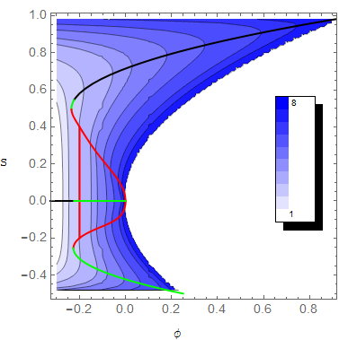
Figure 1: (color online) Equilibrium order parameter $S$ vs. $\phi$ with uniaxial solutions only, superimposed on the energy per particle contours. The black curve represents the stable branch of the bifurcation, the green (light gray) curves correspond to the metastable branches, and the red (dark gray) curves to the unstable branches.

Fig. 1 illustrates our key result. It shows the equilibrium uniaxial order parameter $S$ vs. $\phi$. The stability of different branches is determined by examining the local convexity of the free energy density. To effectively illustrate this, the contours of free energy per particle are superimposed on the bifurcation graph in the $S-\phi$ plane. The black curve represents the stable branch. The green (light gray) curves correspond to metastable states, and the red (dark gray) curves indicate unstable regimes. For $\phi<\phi_{NI}=-0.224$, the system is in the isotropic state with $S=0$; at $\phi=\phi_{NI},$ the system undergoes a first order transition to the nematic state, with order parameter $S_{NI}=0.545$. As $\phi\rightarrow 1$, the order parameter $S\rightarrow 1$ indicating a completely aligned configuration. Inside the blue parabola are the regions where the order parameters of the ordered state are not admissible. At $\phi=-0.2$, the vertical red (dark gray) line indicates that all values of $-0.2<S<0.4$ share the same energy.

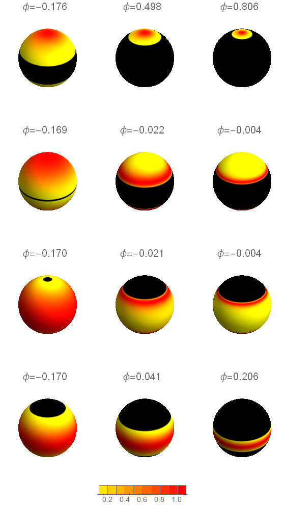
Figure 2: (color online) Density plot of the orientational distribution function for selected equilibrium uniaxial solutions. Top row: stable configuration with order parameter $S>0$; Second row: unstable configuration with $S>0$; Third row: Unstable saddle point configuration with $S<0$; Bottom row: metastable configuration with $S<0$.

In Fig. 2, representative orientational probability density functions are presented as a density plot on the surface of a unit sphere for different equilibrium uniaxial solutions shown on Fig. 1. In those graphs, the $z-$axis is chosen to be along the uniaxial director, thus the density plots are axi-symmetric with respect to the $z-$axis. The density functions are continuous, and normalized by their maximum values on each sphere. The black regions on different spheres indicate forbidden orientations, i.e., no particles are allowed to orient in directions corresponding to those regions. Yellow (light gray) indicates that only relatively few particles are oriented in that direction, and red (dark gray) indicates that the majority of particles are oriented in that direction. The figures clearly reveal that the allowed regions of orientation shrink as the number density increases. This effect is further illustrated in Fig. 3.

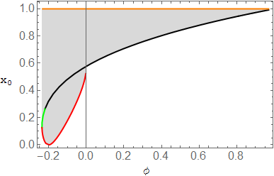
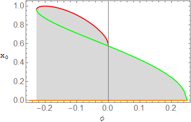
Figure 3: (color online)(a) Lower integration limit $x_{0}$ vs. $\phi$ for uniaxial equilibrium solutions with $S>0$; and the top horizontal line indicates the upper limit of the integration. (b) Upper limit $x_{0}$ vs. $\phi$ for equilibrium solutions with $S<0$; and the bottom horizontal line indicates the lower limit of the integration. Black, green (light gray) and red (dark gray) colors correspond to stable, metastable, and unstable solutions in Fig. 1.

Fig. 3 shows the lower (upper) limit $x_{0}$ of the integration for $S>0$ $(S<0)$. The probability distribution function has no forbidden region when $\Psi=0$. As one traces the stable black branch (Fig. 3a) in the direction of increasing $\phi$, the region shrinks. As $\phi\rightarrow 1$, the lower limit $x_{0}\rightarrow 1$, which implies that all particles orient precisely in the same direction, that is, they are perfectly ordered. At the lowest green (light gray) branch ((Fig. 3b)), as $\phi\rightarrow 1/4$, the upper limit $x_{0}\rightarrow 0,$ the particles all lie in the plane perpendicular to the unique direction (normal to the plane), but are randomly oriented in that plane. On the unstable red (dark gray) branches (Fig. 3ab), the particles are oriented inside or outside a cone, but more towards the boundary of that cone, as shown in the second and third rows in Fig. 2.

IV.3 Phase coexistence

For completeness, we next briefly inquire about the possibility of coexisting nematic and isotropic phases in regions of $\phi$ where both isotropic and nematic solutions exist. We ask therefore whether the total free energy of the system can be reduced by phase separation. Rather than plotting the free energy density versus the number density, as is customary, In Fig. 4 we plot the free energy per particle $\mathcal{F}/\rho_{0}$ versus $\phi$, and implement the classical double tangent construction. Here the common slope indicates equal pressures, and the linear dependence indicates equal chemical potentials of the two coexisting phases. Using this representation, we learn that the nematic and isotropic phases coexist with the universal dimensionless parameter values $\phi_{I}=-0.3652$ and $\phi_{N}=0.1634$, regardless of particle aspect ratio. The phase transition for the homogeneous nematic phase occurs at $\phi_{NI}=-0.224$.

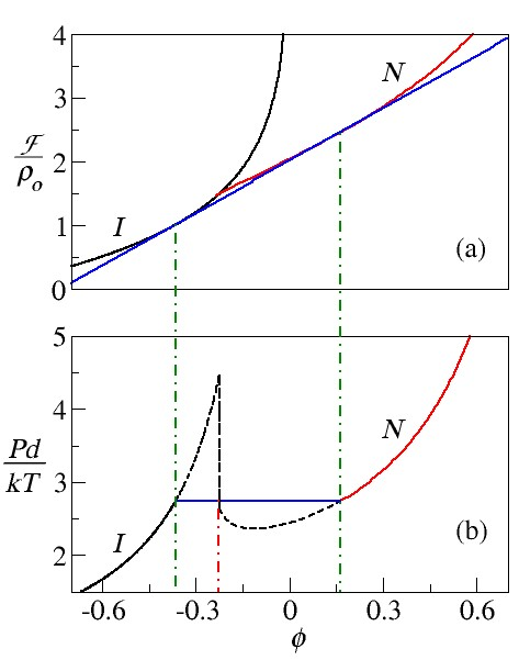
Figure 4: (color online) These diagrams illustrates two-phase coexistence: (a) shows the double tangent construction; (b) shows the Maxwell, equal area construction. The dependence of pressure on $\phi$ in the isotropic and nematic phases is also shown in (b).

The volume fractions $\eta=\rho_{0}v_{0}$ of the two coexisting phases as function of the aspect ratio $\kappa$ can be obtained at once from the values of $\phi_{I}$, and $\phi_{N}$ though Eq. (38), once $\lambda$ is assigned.

V Biaxial equilibrium solutions

We anticipate the existence of biaxial equilibrium solutions, especially for $\phi>0$, since the energy graph for each $\phi>0$ corresponds to two separated branches, with inadmissible regions in between. The energy diverges as $S$ gets near the boundary of the inadmissible region as seen in Fig. 1. If the system starts with a configuration with $S<0$ near the metastable phase, it has to make its way to the lowest energy state, and the only way is through biaxial phases. In its eigenframe, $\mathbf{Q}$ can be represented as

$$\mathbf{Q}=\mathrm{diag}\left[r\cos\left(\alpha+\frac{2\pi}{3}\right),r\cos\left(\alpha-\frac{2\pi}{3}\right),r\cos\alpha\right],$$ (74)

thus $\mathbf{Q}$ is fully characterized by the parameters $r$ and $\alpha$ Zheng&P11 . We use a ternary diagram to represent $\mathbf{Q}$. Consider an equilateral triangle with sides of unit length, centered on the origin, with one vertex on the positive $y-$axis. Each point in the triangle corresponds to a set of eigenvalues of $\mathbf{Q}$. To obtain the eigenvalues of $\mathbf{Q}$, we draw lines parallel to each edge, through the point. Each line intersects two edges, the length of the line segment from the point of intersection to the vertex gives the eigenvalues of $\mathbf{Q}+\frac{1}{3}\mathbf{I}$. We illustrate this in Fig. 5. Due to symmetry, we only consider the shaded $1/6^{th}$ portion of the triangle; and the rest corresponds to $5$ different permutations of the same sets of eigenvalues of $\mathbf{Q}$. Given two coordinates $(x,y)$, $0<x<\sqrt{3}/2$, $-1/2<y<\sqrt{3}x/3$, of a point, $r$ and $\alpha$ can be obtained from

$$r =\sqrt{x^{2}+y^{2}}=\sqrt{\frac{2}{3}\mathbf{Q}:\mathbf{Q}},$$ (75)

$$\alpha =-\frac{\pi}{6}-\arctan\frac{y}{x}.$$ (76)

Here $r=0$, for which $\mathbf{Q}=\mathrm{diag}(0,0,0)$, corresponds to the isotropic phase (the upper left corner of the shaded triangle in Fig. 5); $\alpha=0,$ for which $\mathbf{Q}=\mathrm{diag}(-r/2,-r/2,r)$, corresponds to uniaxial prolate phases (the hypotenuse), and $\alpha=\pi/3$ , for which $\mathbf{Q}=\mathrm{diag}(-r,r/2,r/2)$, corresponds to uniaxial oblate phases (the short vertical edge); $\alpha=\pi/6,$ for which $\mathbf{Q}=\mathrm{diag}(-\sqrt{3}r/2,0,\sqrt{3}r/2)$ , correspond to biaxial phase with largest biaxiality.

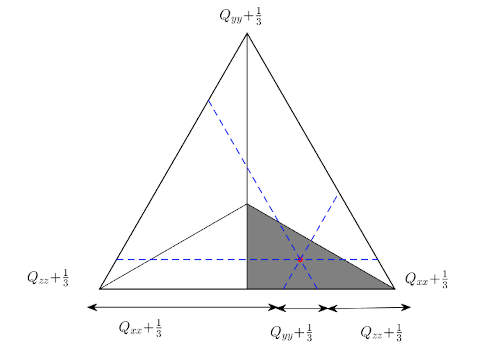
Figure 5: (color online) Ternary diagram for representing $\mathbf{Q}$.

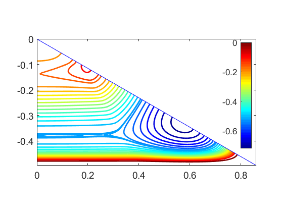
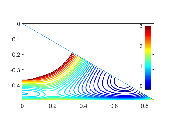
Figure 6: (color online) Energy contours for two representative volume fractions. (a) $\phi=-0.1$; (b) $\phi=0.1$.

We select two representative values of $\phi$ to examine the landscape of the free energy density vs. $\mathbf{Q}$. For each value of $\phi$, we specify $\mathbf{Q}$, and numerically solve for $\mathbf{\Psi}$ using an iterative Newton’s method, and then numerically evaluate the energy density. In Fig. 6, energy density contours are plotted vs. different $\mathbf{Q}$. For $\phi=-0.1$, there are six critical points on the energy surface: one isotropic local minimizer, one prolate uniaxial global minimizer, one uniaxial oblate local maximizer along the hypotenuse, one uniaxial oblate local minimizer, one uniaxial oblate saddle point along the short vertical edge, and one biaxial saddle point in the interior of the triangle. For $\phi=0.1$, there are three critical points: one uniaxial prolate local minimizer along the hypotenuse, one uniaxial oblate local minimizer along the short vertical edge, and one biaxial saddle point in the interior of the triangle. The energy blows up when $r^{2}<\phi$, so there is an inadmissible region in the upper left portion of the triangle. In the regime where $\phi>0$, and the $S<0$ equilibrium solution is stable to biaxial perturbations, we expect a saddle-point corresponding to a “mountain pass” between the $S>0$ and $S<0$ local minimizers. As we have demonstrated there are no other uniaxial critical points in this regime, this saddle-point must be biaxial. Such behavior was not reported in Onsager’s work, nor, as far as we know, in any model for uniaxial particles without an external field.

VI Comparison with simulations

Since the early times of Frenkel and Mulder’s simulations with rotationally symmetric ellipsoids Frenkel85 , this system of hard particles has become the test case for all theories that have attempted to explain the behavior of dense nematics; we could not elude such a test.

Much is known now about the ordering transitions that take place in this system as the number density is increased, including exotic crystal phases, such as the newly discovered SM2 phase donev:unusual ; pfleiderer:simple ; radu:solid , which supplements the stretched fcc-structure already known from Frenkel85 . New points on the isotropic-to-nematic transition line of the phase diagram have also been added for larger values of the aspect ratio $\kappa$ in camp:isotropic and odriozola:revisiting . This latter also presents a full account on all the phases presently known, enriching with new details the bell-shaped diagram already hypothesized in Frenkel85 (see, in particular, Fig. 5 of odriozola:revisiting ). Such a diagram has also proven to be relevant to dynamical studies de_michele:dynamics ; de_michele:simulation , as its shape is reflected by the rotational isodiffusivity lines in the $(\kappa^{-1},\eta)$ plane, where $\eta=\rho_{0}v_{0}$ is the volume fraction. It was shown in these studies how the isotropic-to-nematic transition is heralded by a progressive hampering of the rotational dynamics, which would lead particles to a complete arrest of the rotational motion, were this not pre-empted by the ordering nematic transition.

Clearly, neither the crystal phases nor the dynamical precursors of the nematic phase are within the reach of our theory. But we can still contrast the latter with the simulation data available for the transition value $\eta_{NI}$ of $\eta$.

It readily follows from Eqs. (38), (32), and (31) that our theory predicts the following dependence for $\eta_{NI}$ on the particles’ anisotropy,

$$\eta_{NI}=\frac{1}{8\lambda}\frac{1}{1+(1-\phi_{NI})\varphi(\epsilon)},$$ (77)

where $\varphi(\epsilon)$ is the shape function expressed explicitly by Eq. (85) in terms of the particles’ eccentricity defined in Eq. (33). Letting $\phi_{NI}=-0.244$, as discussed above, we can use Eq. (77) to determine $\lambda$ so as to fit the data available from simulations for the isotropic-to-nematic transition. The comparison of the graph of $\eta_{NI}$ with $41$ data points taken from Frenkel85 , camp:isotropic , and odriozola:revisiting is shown in Fig. 7.

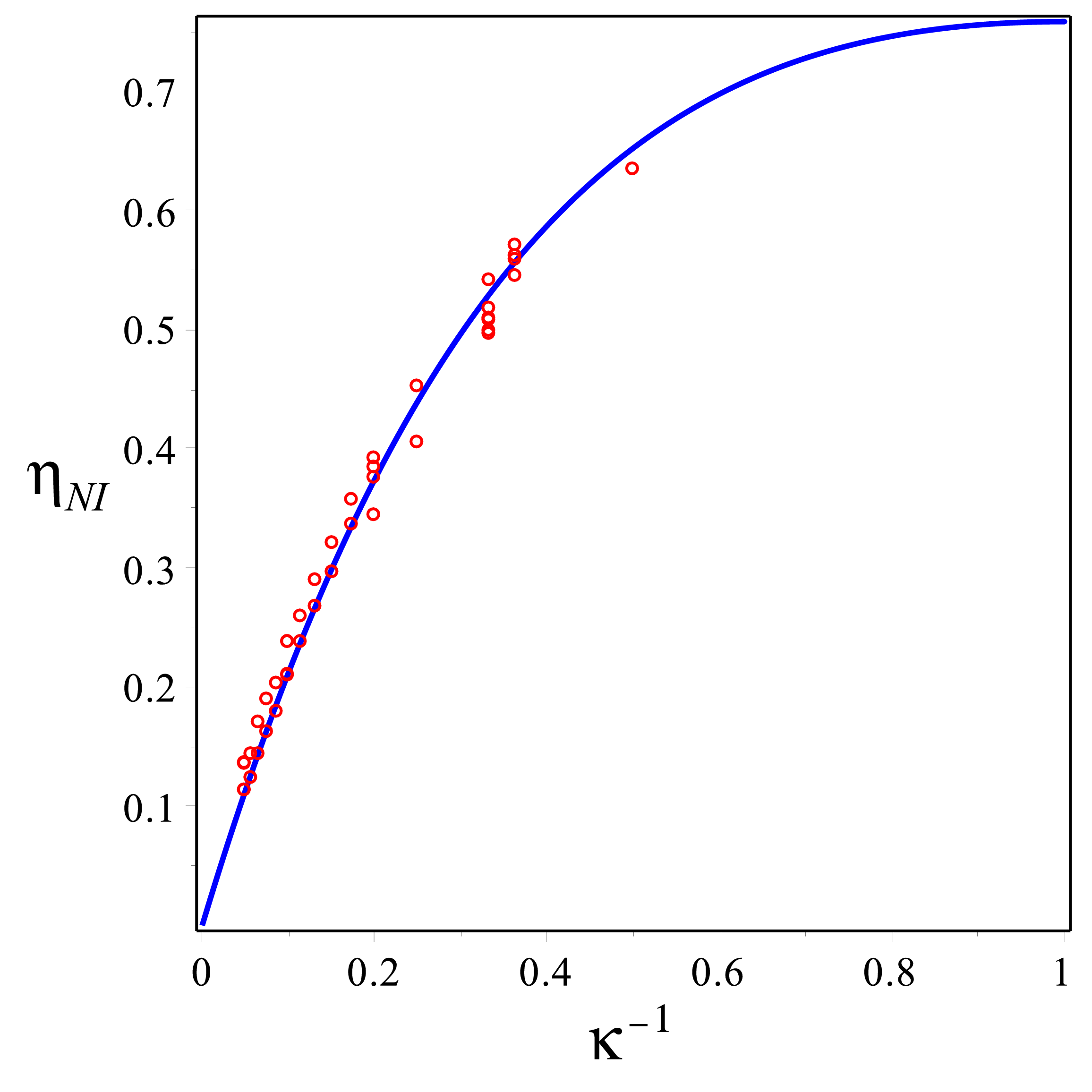
Figure 7: (color online) The graph of $\eta_{NI}$ as in Eq. (77) against the reciprocal $\kappa^{-1}$ of the aspect ratio for $\lambda$ as in Eq. (78). Simulation data are represented by red circles. Data have been collected from Frenkel85 and odriozola:revisiting for both prolate and oblate ellipsoids, and reported here for the effective aspect ratio $\kappa>1$ (which is the real aspect ratio for prolate ellipsoids and its reciprocal for oblate ellipsoids). Data taken from Frenkel85 (see the first two columns of their Table 7) and from camp:isotropic (see the fifth and eighth columns of their Table VI, where $\rho_{\mathrm{cp}}=\sqrt{2}$ ) include both ends of the coexistence range (and their $\eta$ values have been multiplied by $\pi/6$ to account for the fact that the data of Frenkel85 and camp:isotropic are scaled to the volume $LW^{2}=6v_{0}/\pi$). Data taken from odriozola:revisiting are all those in the first column of Table I, but the two referring to the cases 1.3:1-prolate and 1:1.3-oblate, as these latter fall inside the crystal region of the phase diagram (as also shown in Fig. 5 of odriozola:revisiting ).

Since $\eta_{NI}$ depends only on the eccentricity $\epsilon$ of the ellipsoids, we have collected data for both prolate and oblate ellipsoids, and plotted them for the effective aspect ratio $\kappa>1$ (which is the real aspect ratio for prolate ellipsoids and its reciprocal for oblate ellipsoids). The best least-squares fit is found for

$$\frac{1}{\lambda}\doteq 6.065,$$ (78)

which is close to the value for close packed spheres in Eq. (15). Setting $\frac{1}{\lambda}=6$ turns Eq. (77) into our explicit, theoretical prediction for the isotropic-to-nematic transition line for a fluid of hard ellipsoids of revolution.

VII Conclusions

In this paper, we proposed a theory for dense nematics whose constituting molecules interact only through the entropic forces arising from mutual interpenetration. Our emphasis was on the behavior at high densities and the effects of the depletion of available orientational states on orientational order.

We studied a system of hard ellipsoidal particles and compared the predictions of our theory with simulation data on the isotropic-to-nematic transition, finding a good agreement for a specific value of a single fitting parameter $\lambda$. This parameter should more generally be a function of the number density. Work to determine the dependence of $\lambda$ on density is currently under way.

Our study was phrased in the canonical ensemble; we derived an expression for the free energy at the van der Waals level. Low density expansions of the logarithmic term agree with the free energy of Onsager Onsager49 and Doi and Edwards (Doi&Edwards, , p. 354). A major challenge was the determination of the orientational distribution function subject to the hard constraint that the number states available to the system be positive. One striking result of this constraint, in the mean field limit, is that at densities above the isotropic-to-nematic transition, the orientational distribution function which minimizes the free energy has a compact support over orientation space. Although strictly forbidden orientations are likely an artefact of our mean field approach, where particles effectively behave identically, we expect that more sophisticated models would similarly show a strong suppression of the corresponding orientational states.

We have found that the quantity $\phi$, related to the orientational relative free volume, is a convenient control parameter characterizing the state of the system, regardless of density or particle aspect ratio. Our model predicted a first order nematic-isotropic phase transition; in a uniform system, the NI transition occurs at $\phi_{NI}=-0.224$. In the regime $-0.3652\leq\phi$ $\leq 0.1634$, the system is unstable, and undergoes phase separation. As $\phi$ and the density increase, the regions of forbidden orientations grow, and the degree of orientational order increases; the system becomes perfectly aligned in the dense packing limit.

The equation of state from our free energy expression is more realistic than Onsager’s in that in our model, the pressure diverges in the dense packing limit; our equation of state shows the individual contributions of positional and orientational entropy to the pressure.

We see this work as providing a starting point towards a more systematic study of dense nematic systems. Future work is aimed at identifying on a first-principles basis the function of density that is to replace the single parameter $\lambda$ that here ensured agreement between theory and simulation data.

Appendix A Excluded volume of ellipsoids of revolution

In this appendix we justify the approximate form for the excluded volume of two congruent ellipsoids of revolution adopted in this paper and we compare it with other approximations used in the literature.

Symmetry demands that the excluded volume of two congruent bodies of revolution be a function $V_{exc}(x)$ of the inner product $x=\mathbf{\hat{l}}_{1}\cdot\mathbf{\hat{l}}_{2}=\cos\theta$ between the unit vectors designating their axes. In general, $V_{exc}$ can be expanded in a series of Legendre polynomials,

$$V_{exc}(x)=\sum_{k=0}^{\infty}B_{k}P_{k}(x).$$ (79)

It was shown in piastra:explicit that for convex particles all $B_{k}$ can be expressed in terms of a countable family of extended invariant Minkowski shape functionals, which can be computed explicitly for special shapes such as circular cones and ellipsoids of revolution. The formula for $B_{0}$, which represents the isotropic average of $V_{exc}$, had been known to be a function of the classical invariant Minkowski functionals at least since the work of Isihara isihara:determination . It is easy to show that all odd-indexed coefficients $B_{k}$ vanish identically for particles that lack shape polarity.

For an ellipsoid of revolution with eccentricity $\epsilon$,

$$B_{0}=\frac{3}{2}v_{0}\left[\frac{4}{3}+\left(1+(1-\epsilon^{2})\frac{\operatorname{arctanh}\epsilon}{\epsilon}\right)\left(1+\frac{\arcsin\epsilon}{\epsilon\sqrt{1-\epsilon^{2}}}\right)\right],$$ (80)

$$B_{2}=\frac{15}{32}v_{0}\frac{1}{\epsilon^{4}}\left(\epsilon^{2}-3+(\epsilon^{2}+3)(1-\epsilon^{2})\frac{\operatorname{arctanh}\epsilon}{\epsilon}\right)\left(3-2\epsilon^{2}+\frac{4\epsilon^{2}-3}{\epsilon\sqrt{1-\epsilon^{2}}}\arcsin\epsilon\right),$$ (81)

where $v_{0}$ is the particle’s volume. The former formula was already given in isihara:determination , while the latter formula coincides with that given in isihara:theory only for oblate ellipsoids (as pointed out in piastra:explicit , where Eq. (81) was established for all ellipsoids of revolution, the formula of isihara:theory for prolate ellipsoids fails to be invariant under the transformation $\kappa\mapsto 1/\kappa$, and it is thus bound to be incorrect).

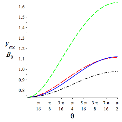
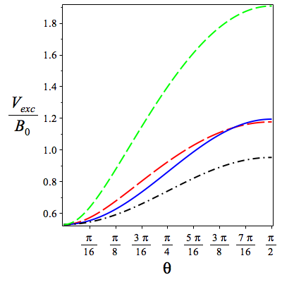
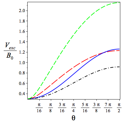
Figure 8: (color online) The excluded volume of a pair of congruent ellipsoids of revolution $V_{exc}$ (normalized to its isotropic average $B_{0}$) is plotted against the angle $\theta$ between their symmetry axes according to four different approximate formulas: (red long-dashed) the expansion in Eq. (79) truncated at $k=20$ with the coefficients computed according to the theory of piastra:explicit ; (blue solid) our approximate formula in Eq. (82); (black dash-dotted) Sheng’s formula from Sheng75 ; (green dashed) the HGO formula in Eq. (89). Values of the ellipsoids’ aspect ratio: (a) $\kappa=3$, (b) $\kappa=5$, (c) $\kappa=10$.

We wish to approximate $V_{exc}(x)$ with

$$V_{exc}^{(\mathrm{app})}(x)=C-DP_{2}(x),$$ (82)

with $C$ and $D$ constants chosen in such a way that

$$V_{exc}^{(\mathrm{app})}(1)=8v_{0}$$ (83)

and

$$V_{exc}^{(\mathrm{app})}(0)=B_{0}+B_{2}P_{2}(0)=B_{0}-\frac{1}{2}B_{2},$$ (84)

where $B_{0}$ and $B_{2}$ are as in Eqs. (80) and (81). It is a simple matter to show that $C$ and $D$ can be written as in Eqs. (31) and (32) with the shape function $\varphi$ defined as

$$\begin{split}\varphi(\epsilon)=\frac{1}{768}\frac{1}{\epsilon^{6}}\Big{\{}&254\epsilon^{6}-135\epsilon^{4}+135\epsilon^{2}+9\epsilon(4\epsilon^{4}+25\epsilon^{2}-15)\frac{\arcsin\epsilon}{\sqrt{1-\epsilon^{2}}}\\ &+9\epsilon(1-\epsilon^{2})(14\epsilon^{4}+5\epsilon^{2}-15)\operatorname{arctanh}\epsilon\\ &+9(1-\epsilon^{2})(4\epsilon^{4}-15\epsilon^{2}+15)\frac{\arcsin\epsilon}{\sqrt{1-\epsilon^{2}}}\operatorname{arctanh}\epsilon\Big{\}}-\frac{2}{3}.\end{split}$$ (85)

In the main text we have adopted the function in Eq. (82) (and dropped the cumbersome superscript ^(app)). The function $\varphi$ is positive and monotonically increasing on the interval $[0,1)$; it diverges as $\epsilon\to 1^{-}$ and possesses the following asymptotic behaviors:

$$\lim_{\epsilon\to 0}\epsilon^{-4}\varphi(\epsilon)=\frac{1}{15},$$ (86)

$$\lim_{\epsilon\to 1^{-}}\sqrt{1-\epsilon^{2}}\varphi(\epsilon)=\frac{21\pi}{256}.$$ (87)

Other approximate formulae have been proposed in the past for the excluded volume of ellipsoids of revolution. Sheng Sheng75 used a formula like the one in Eq. (82), for which $\varphi$ would be replaced by the following simpler form,

$$\varphi(\epsilon)=\frac{\left(\sqrt{1-\epsilon^{2}}-1\right)^{2}}{\sqrt{1-\epsilon^{2}}}.$$ (88)

Berne and Penchukas berne:gaussian introduced the Hard Gaussian Overlap model (customarily abbreviated HGO in the literature), which mimics a short range repulsion between elongated molecules (see de_miguel:isotropic for a lucid description of this model and its connections with traditional hard-particle models). When applied to hard ellipsoids, this model delivers an effective excluded volume written in the form

$$V_{exc}^{\mathrm{(HGO)}}(x)=8v_{0}\sqrt{\frac{1-\chi^{2}x^{2}}{1-\chi^{2}}},\quad\text{where}\quad\chi^{2}=\frac{\kappa^{2}-1}{\kappa^{2}+1}.$$ (89)

It is instructive to compare our approximate formula in Eq. (82), Sheng’s variant, and the HGO formula with the remarkably good (at least for $\kappa\leq 20$), but highly inconvenient expression obtained from Eq. (79) by truncating the series expansion at $k=20$ and computing its coefficients exactly through the theory presented in piastra:explicit . Figure 8 illustrates such a comparison for $\kappa=3$, $5$, and $10$. While the HGO formula highly overestimates the excluded volume, Sheng’s formula underestimates it (though less dramatically so). By contrast, the formula we have used in this study seems to be more faithful, at least to the truncated Legendre expansion.

References

- (1) Frenkel, D., McTague, J. P., and Mulder, B. M., Phase diagram of a system of hard ellipsoids, Phys. Rev. Lett., 52, 287–290 (1984).
- (2) Frenkel, D., and Mulder, B. M., The hard ellipsoid-of-revolution fluid: I. Monte Carlo simulations, Mol. Phys. 55 (5), 1171–1192 (1985).
- (3) Mulder, B. M., and Frenkel, D., The hard ellipsoid-of-revolution fluid: II. The -expansion equation of state, Mol. Phys., 55, 1193–1215 (1985).
- (4) Onsager, L., The effects of shape on the interaction of colloidal particles. Ann. N. Y. Acad. Sci., 51, 627–659 (1949).
- (5) Palffy-Muhoray, P., Virga, E. G., and Zheng, X., Towards Onsager’s density functional via Penrose’s tree indentity, to be submitted (2017).
- (6) Mederos, L., Velasco, E., and Martinez-Raton, Y., Hard-body models of bulk liquid crystals, J. Phys.: Condens. Matter, 26, 463101 (2014).
- (7) Mayer, J. E., and Mayer, M. G., Statistical Mechanics, (Wiley, New York, 1940).
- (8) Straley, J. P., The gas of long rods as a model for lyotropic liquid crystals, Mol. Cryst. Liq. Cryst., 2, 333–357 (1973).
- (9) Straley, J. P., Third virial coefficient for the gas of long rods, Mol. Cryst. Liq. Cryst., 24, 7–20 (1973).
- (10) Tjipto-Margo, B., and Evans, G. T., The Onsager theory of the isotropic-nematic liquid crystal transition: incorporation of the higher virial coefficients, J. Chem. Phys., 93, 4254–5265 (1990).
- (11) Barboy, B., and Gelbart, W. M., Series representation of the equation of state for hard particle fluids, J. Chem. Phys., 71, 3053–3026 (1979).
- (12) Barboy, B., and Gelbart, W. M., Hard-particle fluids. II. General -expansion-like descriptions, J. Stat. Phys., 22, 709–742 (1980).
- (13) R. Zwanzig, First-order phase transition in a gas of long thin rods, J. Chem Phys., 39, 1714–1721 (1963).
- (14) Parsons, J. D., Nematic ordering in a system of rods, Phys. Rev. A, 19, 1225–1230 (1979).
- (15) Lee, S.-D., A numerical investigation of nematic ordering based on a simple hard-rod model, J. Chem. Phys., 87, 4972–4974 (1987).
- (16) Carnahan, N. F., and Starling, K. E., Equation of state for nonattracting rigid spheres, J. Chem. Phys., 51, 635–636 (1969).
- (17) Lee, S.-D., The Onsager-type theory for nematic ordering of finite-length hard ellipsoids, J. Chem. Phys., 89, 7036–7037 (1988).
- (18) Baus, M., Colot, J.-L., Wu, X.-G., and Xu, H., Finite-density Onsager-type theory for the isotropic-nematic transition of hard ellipsoids, Phys. Rev. Lett., 59, 2184–2187 (1987).
- (19) Colot, J.-L., Wu, X.-G., Xu, H., and Baus, M., Density-functional, Landau and Onsager theories of the isotropic-nematic transition of hard-ellipsoids, Phys. Rev. A, 38, 2022–2036 (1988).
- (20) Palffy-Muhoray, P., and Bergersen, B., van der Waals theory for nematic liquid crystals, Phys. Rev. A, 35, 2704–2708 (1987).
- (21) Sheng, P., Hard rod model of the nematic-isotropic phase transition, in Introduction to Liquid Crystals, Priestley, E. B., Wojtowicz, P. J., Sheng, P., Eds., pp. 59–70, (Plenum Press, Boston, 1974).
- (22) Taylor, M. P., and Herzfeld, J., Nematic and smectic order in a fluid of biaxial hard particles, J, Phys. Rev. A, 44, 3742–3751 (1991).
- (23) Malijevsky, A., Jackson, G., and Varga, S., Many-fluid Onsager density functional theories for orientational ordering in mixtures of anisotropic hard-body fluids, J. Chem. Phys., 129, 144504 (2008).
- (24) Wu, L., Malijevsky, A., Jackson, G., Muller, E. A., and Avendano, C., Orientational ordering and phase behaviour of binary mixtures of hard spheres and hard spherocylinders, J. Chem. Phys., 143, 044906 (2015).
- (25) Israelachvili, J. N., Intermolecular and Surface Forces, (Academic Press, Waltham, 1992).
- (26) Gartland, E. C. Jr., and Virga, E. G., Minimum principle for indefinite mean-field free energies, Arch. Rational Mech. Anal., 196, 143–189 (2010).
- (27) Palffy-Muhoray, P., The single particle potential in mean-field theory, Am. J. Phys., 70, 433–437(2002).
- (28) Sonnet, A. M., and Virga, E. G., Dissipative Ordered Fluids: Theories for Liquid Crystals, (Springer, New York, 2012).
- (29) Doi, M., and Edwards, S. F., The Theory of Polymer Dynamics, (Clarendon Press, Oxford, 1988).
- (30) van Kampen, N. G., Condensation of a classical gas with long range attraction, Phy. Rev., 135, A362–A369 (1964).
- (31) Tonks, L., The complete equation of state of one, two and three-dimensional gases of hard elastic spheres, Phys. Rev., 50, 955–963 (1936).
- (32) Taylor, J. M., An analysis of equilibria in dense nematic liquid crystals, arXiv:1702.08793.
- (33) Maier, W., and Saupe, A., Eine einfache molekulare Theorie des nematischen kristallinflüussigen Zustandes, Z. Naturforsch A, 13(a), 564–566 (1958).
- (34) Fatkullin, I., and Slastikov, V., Critical points of the Onsager functional on a sphere, Nonlinearity, 18, 2565–2580 (2005).
- (35) Zheng, X., and Palffy-Muhoray, P., One order parameter tensor mean field theory for biaxial liquid crystals, Discrete Contin. Dyn. S. B, 15, 475–490 (2011).
- (36) Pfleiderer, P., and Schilling, T., Simple monoclinic crystal phase in suspensions of hard ellipsoids, Phys. Rev. E, 75, 020402(R) (2007).
- (37) Donev, A., Stillinger, F. H., Chaikin, P. M., and Torquato, S., Unusually dense crystal packings of ellipsoids, Phys. Rev. Lett., 92, 255506 (2004).
- (38) Radu, M., Pfleiderer, P., and Schilling, T., Solid-solid phase transition in hard ellipsoids, J. Chem. Phys., 131, 164513 (2009).
- (39) Camp, P. J., Mason, C. P. , Allen, M. P., Khare, A. A., and Kofke, D. A., The isotropic-nematic phase transition in uniaxial hard ellipsoid fluids: Coexistence data and the approach to the Onsager limit, J. Chem. Phys., 105, 2837–2849 (1996).
- (40) Odriozola, G., Revisiting the phase diagram of hard ellipsoids, J. Chem. Phys., 136, 134505 (2012).
- (41) De Michele, C., Schilling, R., and Sciortino, F., Dynamics of uniaxial hard ellipsoids, Phys. Rev. Lett., 98, 265702 (2007).
- (42) De Michele, C., Schilling, R., and Sciortino, F., Simulation of the dynamics of hard ellipsoids, Phil. Mag., 88, 4117–4123 (2008).
- (43) Piastra, M., and Virga, E. G., Explicit excluded volume of cylindrically symmetric convex bodies, Phys. Rev. E, 91, 062503 (2015).
- (44) Isihara, A., Determination of molecular shape by osmotic measurement, J. Chem. Phys., 18, 1446–1449 (1950).
- (45) Isihara, A., Theory of anisotropic colloidal solutions, J. Chem. Phys., 19, 1142–1147 (1951).
- (46) Berne, B. J., and Penchukas, P., Gaussian model potentials for molecular interactions, J. Chem. Phys., 56, 4213–4216 (1971).
- (47) de Miguel, E., and Martín del Río, E., The isotropic-nematic transition in hard Gaussian overlap fluids, J. Chem. Phys., 115, 9072 (2001).