Prospects of detecting HI using redshifted $21$ cm radiation at $z\sim 3$

Abstract

Distribution of cold gas in the post-reionization era provides an important link between distribution of galaxies and the process of star formation. Redshifted $21$ cm radiation from the Hyperfine transition of neutral Hydrogen allows us to probe the neutral component of cold gas, most of which is to be found in the interstellar medium of galaxies. Existing and upcoming radio telescopes can probe the large scale distribution of neutral Hydrogen via HI intensity mapping. In this paper we use an estimate of the HI power spectrum derived using an ansatz to compute the expected signal from the large scale HI distribution at $z\sim 3$. We find that the scale dependence of bias at small scales makes a significant difference to the expected signal even at large angular scales. We compare the predicted signal strength with the sensitivity of radio telescopes that can observe such radiation and calculate the observation time required for detecting neutral Hydrogen at these redshifts. We find that OWFA (Ooty Wide Field Array) offers the best possibility to detect neutral Hydrogen at $z\sim 3$ before the SKA (Square Kilometer Array) becomes operational. We find that the OWFA should be able to make a $3\,\sigma$ or a more significant detection in $2000$ hours of observations at several angular scales. Calculations done using the Fisher matrix approach indicate that a $5\sigma$ detection of the binned HI power spectrum via measurement of the amplitude of the HI power spectrum is possible in $1000$ hours (Sarkar, Bharadwaj and Ali, 2017).

Keywords: cosmology: large scale structure of the universe, galaxies: evolution, radio-lines: galaxies

1 Introduction

It is believed that the formation of galaxies in dark matter halos led to emission of UV radiation that gradually ionized the inter-galactic medium (IGM) by $z\simeq 6$ (Zaroubi, 2013). The IGM is almost fully ionized at lower redshifts, and nearly all the neutral Hydrogen in the universe is to be found in the inter-stellar medium (ISM) of galaxies (Wolfe, Gawiser, & Prochaska, 2005; Carilli & Walter, 2013). This allows us to model the distribution of neutral gas in terms of assignment schemes that apportion the neutral gas in halos of dark matter. Such a model can then be constrained by observations of damped Lyman $\alpha$ systems (DLAS) seen as strong absorption in the spectra of quasars at high redshifts (Villaescusa-Navarro et al., 2014; Padmanabhan, Choudhury, & Refregier, 2015). The observations of DLAS indicate that at redshifts $2\leq z\leq 5$, the neutral hydrogen content of the universe is almost constant with a density parameter ${\Omega}_{HI}\sim 0.001$ (Noterdaeme et al., 2012). Clustering of DLAS has been used to constrain the bias for these objects (Font-Ribera et al., 2012) and it appears that these objects are strongly clustered when compared with the matter distribution at these redshifts.

Several upcoming radio telescopes can be used to detect neutral Hydrogen at high redshifts using the redshifted $21$ cm radiation using intensity mapping (Bharadwaj & Sethi, 2001; Santos et al., 2015; Tingay et al., 2013). The focus of the present study is at redshift $z\simeq 3$. A number of telescopes can potentially detect redshifted $21$ cm from neutral Hydrogen at high redshifts: GMRT (Giant Meterwave Radio Telescope), uGMRT (upgraded GMRT), OWFA (Ooty Wide Field Array), MWA (Murchison Widefield Array), CHIME (Canadian Hydrogen Intensity Mapping Experiment) and SKA-low. The focus of the present study is $z\sim 3$. Thus we discuss the feasibility of detecting redshifted $21$ cm radiation using the GMRT, MWA, SKA and OWFA as these instruments can target this redshift range. The analysis is not meant to be exhaustive but a broad brush comparison of these instruments.

In this paper we use the model suggested by Bagla, Khandai, & Datta (2010) for populating dark matter halos with neutral Hydrogen. We then proceed to compute the expected signal and compare this with the sensitivity of several radio telescopes. This comparison is done using the approach used in (Ali & Bharadwaj, 2014). We do not consider the foregrounds in this paper, readers may refer to Ali & Bharadwaj (2014) for a discussion and references.

2 Methodology

The observables in the context of the HI intensity mapping are visibility correlations and these have been shown to be related to the redshift space power spectrum of HI fluctuations (Bharadwaj & Sethi, 2001; Chang et al., 2008) in the limit of a small field of view. A physically motivated scheme to populate dark matter halos with neutral Hydrogen has been used in the past for modelling the HI power spectrum (Bagla, Khandai, & Datta, 2010) and similar results for clustering are obtained in the halo model with a similar approach (Wyithe & Brown, 2010). This model is able to reproduce the column density distribution of DLAS (Villaescusa-Navarro et al., 2014; Padmanabhan, Choudhury, & Refregier, 2015), though it seems to under-predict the bias for DLAS as compared to recent observational determination (Font-Ribera et al., 2012).

In this paper we use a fitting function for the HI power spectrum in order to estimate the signal in redshifted $21$ cm radiation from the large scale distribution of HI at $z\sim 3$. This approach uses the linearly evolved matter power spectrum and a fitting function for a scale dependent bias and non-linear evolution, where the fitting function is obtained from N-Body simulations (Bagla, Khandai, & Datta, 2010). Figure 1 shows the power spectrum for the HI distribution as obtained from N-Body simulations. For ease of computation, we do not use the conventional bias but work instead with the offset between the HI power spectrum and the linearly extrapolated power spectrum for dark matter: thus it gives the combined effect of non-linear growth of perturbations as well as a scale dependent bias. One immediate benefit of this approach is that we are not limited to the scales resolved in simulations used to derive the HI power spectrum. There is a need to excercise caution when extrapolating to smaller scales as we know little about the scale dependence of bias at these scales from N-Body simulations. However, in this work we are analyzing signal primarily at large angular scales and hence the effect of errors in modelling scales smaller than those resolved in simulations can be shown to be minimal.

The HI content of galaxies at very low redshifts can be estimated directly from observed emission of $21$ cm radiation (Zwaan et al., 2005; Giovanelli & Haynes, 2016). This radiation arises from the Hyperfine transition of neutral Hydrogen (Wild, 1952; van de Hulst, Raimond, & van Woerden, 1957) and if the spin temperature is much higher than the temperature of the CMBR (cosmic microwave background radiation) then the emission is proportional to the amount of neutral Hydrogen (Furlanetto, Oh, & Briggs, 2006). The spin temperature in turn is determined by coupling with atoms, electrons and Lyman-$\alpha$ line radiation (Wouthuysen, 1952b, a; Purcell & Field, 1956; Furlanetto, Oh, & Briggs, 2006). At intermediate redshifts, techniques such as co-adding (Chengalur, Braun, & Wieringa, 2001; Zwaan, 2000; Lah et al., 2007; Rhee et al., 2013; Delhaize et al., 2013; Rhee et al., 2016; Kanekar, Sethi, & Dwarakanath, 2016) and cross-correlation (Chang et al., 2010; Masui et al., 2013) have been used to detect neutral Hydrogen. As we get to even higher redshifts, statistical detection is the only viable approach for observing the large scale distribution of HI. The collective emission from the undetected regions is present as a very faint background in all radio observations at frequencies below $1420$ MHz. The fluctuations in this background radiation carry an imprint of the HI distribution at the redshift $z$ where the radiation originated. HI emission from the post-reionization era can be used as a probe of the large scale structure and can also be used to constrain cosmological paramters (Bharadwaj & Sethi, 2001; Bharadwaj, Sethi, & Saini, 2009; Pritchard & Loeb, 2012). It should be noted though that the possibility of direct detection of extreme objects (Bagla, Nath, & Padmanabhan, 1997) should not be discounted, particularly in the light of very high bias at small scales (Bagla, Khandai, & Datta, 2010; Wyithe & Brown, 2010).

Realizing the potential for constraining cosmological parameters, the majority of the existing and upcoming radio-interferometric experiments such as LOFAR, MWA, SKA, PAPER, etc. are aimed at measuring the HI 21 cm signal statistically and map out the large scale HI distribution at high redshifts with the primary focus on the epoch of reionization. Similarly CHIME is an experiment for detecting post-reionization distribution of HI at large scales. The Ooty Wide Field Array (OWFA) (Bargur et al., 2011; Subrahmanya, Manoharan and Chengalur, 2017) is the upgraded Ooty radio telescope where the collecting area and the primary receivers remain the same but the entire backend has been changed. OWFA has a much larger field of view and a much larger bandwidth as compared to the earlier configuration. A new programmable backend has been added to the existing capability. For details, please see (Swarup et al., 1971; Kapahi et al., 1975; Sarma et al., 1975; Joshi et al., 1988; Prasad & Subrahmanya, 2011; Subrahmanya, Manoharan and Chengalur, 2014, 2017). OWFA has the potential of detecting HI at $z\simeq 3$ and also measuring the power spectrum (Ali & Bharadwaj, 2014).

3 Ooty Wide Field Array

OWFA consists of a parabolic cylindrical antenna which is $530$ m long in north-south direction and $30$ m wide in east-west direction. It is an equatorially mounted phased array of $1056$ dipoles placed along the focal line of the reflector. The East-West steering (RA) is done by the mechanical rotation of the telescope about its N-S axis and steering of beam in north-south direction (Declination) is achieved by introducing appropriate delays between the dipoles. The array possesses huge redundancy (different antenna pairs correspond to same baseline) due to its linearity and uniform spacing of the antenna elements (Prasad & Subrahmanya, 2011). This redundancy is very useful for precision experiments, since it allows for model independent estimation of both the element gains as well as true visibilities (Wieringa, 1991, 1992; Liu et al., 2010; Marthi & Chengalur, 2014). The array has been upgraded to improve sensitivity and the Field of View (FoV). It can now be used as an interferometer and has multibeaming feature.

OWFA has $264$ antenna elements and each element can be approximated as a rectangular aperture dimensions(b $\times$ d) equal to $30$ m $\times$ $1.92$ m. The primary field of view is about $1.75$° in E-W direction and $27.4$° in N-S direction with a resolution of $0.1$°. The smallest baseline corresponds to antenna separation of $1.92$ m and the largest baseline is $505$ m. Total bandwidth of the system is $39$ MHz.

The upgraded array is sensitive primarily to HI power spectrum at wave numbers between $0.02-0.2$ h$/$Mpc (Bharadwaj, Sarkar, & Ali, 2015; Sarkar, Bharadwaj and Ali, 2017). The observable signal here is the visibility correlation and it is related to an integral over the power spectrum and hence it has some contribution from power spectrum at other scales (Bharadwaj & Sethi, 2001; Bharadwaj & Ali, 2005).

If we compare OWFA with the other radio telescopes that are, or will be, sensitive to redshifted $21$ cm radiation from $z\sim 3$ then we find that each has its own peculiarities.

• GMRT has a very large collecting area and hence very good sensitivity. However, the primary beam is very small as the size of the dish is large at $45$ m.

• MWA has a small effective collecting area but the field of view is large and it is sensitive to signal at a wide range of angular scales.

• SKA-Low is in some sense akin to MWA but with a much larger collecting area.

Table 1: System parameters for OWFA

Parameter	OWFA
No. of antennas ($N_{A}$)	264
Aperture dimensions ($b\times d$)	$30$ m $\times$ $1.92$ m
Field of View(FoV)	$1.75$°$\times$ $27.4$°
Smallest baseline ($d_{min}$)	$1.92$ m
Largest baseline ($d_{max}$)	$505.0$ m
Angular Resolution	$1.75^{\circ}\times 6.3^{\prime}$
Total Bandwidth (B)	$30$ MHz
Single Visibility rms. noise ($\sigma$) assuming $T_{sys=}$ 150 K, $\eta=$ 0.6, $\Delta\nu_{c}=$ 0.1 MHz, $\Delta t=$ 16 s	6.69 Jy

4 Visibility correlations and HI Power Spectrum

The multi-frequency angular power spectrum $C_{l}(\Delta\nu)$ can be used to quantify the statistical properties of the signal observed on the sky. It is a function of the angular scale $l$ and frequency shift $\Delta\nu$. The observed visibilities ${\cal V}(U_{n},\Delta\nu)$ are related to $C_{l}(\Delta\nu)$ through the visibility correlation which can be written as (Datta, Choudhury, & Bharadwaj, 2007)

$$C_{l}(\Delta\nu)=0.26\ {\left(\dfrac{\text{mK}}{\text{Jy}}\right)}^{2}\left(\dfrac{bd}{m^{2}}\right)V_{2}(U_{n},\Delta\nu)$$ (1)

Where

$$V_{2}(U_{n},\Delta\nu)\equiv\langle{\cal V}(U_{n},\nu){\cal V}^{*}(U_{m},\nu+\Delta\nu)\rangle$$ (2)

is the visibility correlation.

Equation (1) provides a reasonably good approximation for the entire baseline range covered by OWFA. The measured visibility correlations are a combination of three different components:

$${V}_{2}(U_{n},\Delta\nu)={S}_{2}(U_{n},\Delta\nu)+{F}_{2}(U_{n},\Delta\nu)+{N}_{2}(U_{n},\Delta\nu)$$ (3)

where $S_{2},F_{2}$ and $N_{2}$ respectively are the HI signal, foreground and the noise contribution to the visibility correlation. In our calculations we have assumed that all foreground signals are already removed from the signal (zero foreground contribution) and treat the total signal as consisting of only HI signal and noise. Removal of foregrounds is an essential and a non-trivial task: see, e.g., (Ali, Bharadwaj & Chengalur, 2008; Ghosh et al., 2011; Ghosh, Koopmans, Chapman & Jelić, 2015). A discussion of foreground removal is beyond the scope of this paper.

${S}_{2}(U_{n},\Delta\nu)$ from the HI signal directly probes the redshift space power spectrum $P_{HI}(\textbf{k},z)$ (Bharadwaj & Sethi, 2001; Bharadwaj & Ali, 2005). The multi-frequency angular power spectrum can be calculated for the HI signal using equation (4).

$$C_{l}(\Delta\nu)=\dfrac{1}{\pi r_{\nu}^{2}}\int_{0}^{\infty}dk_{||}\text{cos}(k_{||}r_{\nu}^{\prime}\Delta\nu)P_{\text{HI}}(\textbf{k})$$ (4)

where k has magnitude $k=\sqrt{k_{\parallel}^{2}+l^{2}/r_{\nu}^{2}}$ and has components $k_{\parallel}$ and $l/r_{\nu}$ along the line of sight and in the plane of the sky respectively. The multipole index $l$ takes on positive integer values. Here $r_{\nu}$ is the comoving distance corresponding to $z=(1420\text{MHz}/\nu)-1$, $r_{\nu}^{\prime}=\frac{dr_{\nu}}{d\nu}$.

Assuming that HI traces the total matter distribution with a bias parameter, $P_{HI}(k,\mu)\equiv P_{HI}(\textbf{k})$ can be modelled as

$$P_{\text{HI}}(k,\mu)=b^{2}\bar{x}_{\text{HI}}^{2}\bar{T}^{2}\left[1+\beta\mu^{2}\right]^{2}P(k)$$ (5)

$$\bar{T}(z)=4.0\text{mK}(1+z)^{2}\left(\dfrac{\Omega_{b}h^{2}}{0.02}\right)\left(\dfrac{0.7}{h}\right)\left(\dfrac{H_{0}}{H(z)}\right)$$ (6)

where $P(k)$ is the matter power spectrum at the redshift $z$, $\bar{x}_{HI}$ is the mean neutral hydrogen fraction. $\mu=k_{\parallel}/k$ is the cosine of angle between k and the line of sight and $\beta$ is the linear distortion parameter. $\beta$ depends on cosmology and bias parameter $b$. The $\mu$ dependence of $P_{HI}(\textbf{k})$ arises from the peculiar velocities and the resulting redshift space distortions (Kaiser, 1987; Zaroubi & Hoffman, 1996). We use $\bar{x}_{HI}=2.45\times 10^{-2}$ and this corresponds to ${\Omega}_{gas}=0.001$ (Noterdaeme et al., 2012; Zafar et al., 2013).

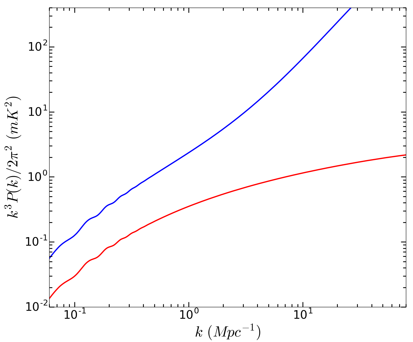
Figure 1: This plot shows the dimensionless power spectrum $\Delta^{2}(k)$ scaled to brightness temperature units. The red curve shows linearly extrapolated WMAP9 matter power spectrum $P(k)$ for the parameters mentioned in the text. The blue curve shows HI power spectrum $P_{HI}(k)$ calculated using the bias model mentioned in eq.(7).

N-body simulations (Bagla, Khandai, & Datta, 2010) provide justification for considering a linear scale independent bias $b\simeq 2$ for $k\ll 1\text{Mpc}^{-1}$ with respect to the linear power spectrum. For $k>1\text{Mpc}^{-1}$, the bias $b$ has a non-linear dependence on $k$. There are two steps involved in the calculation of the HI power spectrum: mapping from the linearly extrapolated dark matter power spectrum to the non-linear power spectrum, and, a scale dependent bias $b(k)$. Both of these are obtained from N-Body simulations, but simulations can access only a finite range of scales. Limiting our calculations to this range of scales introduces oscillations in the computed signal hence it is essential to model these over the entire range of scales. We choose to do so by fitting a function relating the linearly evolved power spectrum with the HI power spectrum as obtained in N-Body simulations.

We have modelled the scale dependence of bias $b\equiv b(k)$ in which $b(k)$ varies with $k$ as

$$b(k)=\dfrac{b_{0}+b_{1}(k/k_{0})}{1+b_{2}(k/k_{1})}$$ (7)

where $b_{0}=2.0,\ b_{1}/k_{0}=0.6\ \text{Mpc}^{-1},\ \&\ b_{2}/k_{1}=0.005\ \text{Mpc}^{-1}$. The parameters are obtained from the HI power spectrum computed using an ansatz in N-Body simulations (Model 2 in Bagla, Khandai, & Datta (2010)). The first two parameters, $b_{0}$ and $b_{1}/k_{0}$ are strongly constrained by the simulation data. $b_{2}/k_{1}$ is not constrained very strongly and we choose a value that fits the data and minimises the impact on the estimated signal. As mentioned above, this bias is defined with respect to the linearly evolved dark matter power spectrum and not the non-linear power spectrum computed from simulations for convenience of calculations. We have employed this scale dependent bias model (eq. 7) to calculate the HI power spectrum (eq. 6) which gives a close approximation to the HI power spectrum calculated using N-body simulations upto $k\sim 10\ \text{Mpc}^{-1}$. We have used the linearly extrapolated WMAP 9 matter power spectrum with $\Lambda$CDM cosmology to calculate HI power spectrum and the corresponding parameters are $H_{0}=70.0\text{Km/s/Mpc},\ {\Omega}_{b}h^{2}=0.02264,\ {\Omega}_{\Lambda}=0.721,n_{s}=0.972,{\sigma}_{8}=0.821$.

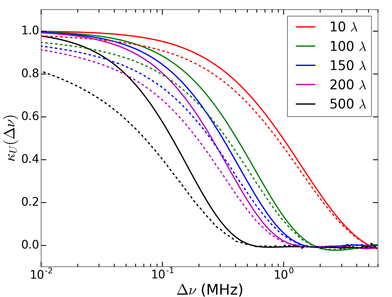
Figure 2: Frequency decorrelation function ${\kappa}_{U}(\Delta\nu)$ as a function of $\Delta\nu$ at five different U values indicated in figure. The signal decorrelates more sharply for higher value of U. Dashed lines show the decorrelation function for the model with scale dependent bias whereas solid lines show the corresponding function for linear bias. It is seen here that the signal remains correlated over a smaller range in frequency for the scale dependent bias model as compared to the linear bias model. This indicates that including the effect of scale dependent bias decreases the frequency correlation of signal. This decrement is more significant at higher values of U.

We use the decorrelation function ${\kappa}_{U}(\Delta\nu)$ to quantify the $\Delta\nu$ dependence of the signal $S_{2}(U,\Delta\nu)$. This allows us to assess the HI signal decorrelation with frequency separation $\Delta\nu$. ${\kappa}_{U}(\Delta\nu)$ can be defined as Datta, Choudhury, & Bharadwaj (2007)

$${\kappa}_{U}(\Delta\nu)=\dfrac{S_{2}(U,\Delta\nu)}{S_{2}(U,0)}$$ (8)

Figure 2 shows ${\kappa}_{U}(\Delta\nu)$ as a function of $\Delta\nu$ for different baselines U. Dashed lines show the variation for the scale dependent bias and solid lines for the constant bias as mentioned above. In both models the bias is applied to the linearly extrapolated power spectrum as this facilitates comparison with results published in Bharadwaj, Sarkar, & Ali (2015). The signal is fully correlated at zero separation, as expected, and we have ${\kappa}_{U}(0)=1$. The correlation falls (${\kappa}_{U}(\Delta\nu)<1$) as $\Delta\nu$ is increased. We see that ${\kappa}_{U}(\Delta\nu)$ varies slowly with $\Delta\nu$ at the small baselines. For $U=10$, we have ${\kappa}_{U}(\Delta\nu)=0.5$ at $\Delta\nu\approx 1\text{MHz}$, beyond which $\kappa$ falls further. At larger baselines, ${\kappa}_{U}(\Delta\nu)$ has a steeper dependence with $\Delta\nu$. For $U=200$, ${\kappa}_{U}(\Delta\nu)=0.5$ at $\Delta\nu\approx 0.2\text{MHz}$, and ${\kappa}_{U}$ crosses zero near $\Delta\nu\approx 1\text{MHz}$. The signal decorrelates faster for the scale dependent bias model where there is more power at small scales. This plot illustrates that the combined boost at small scales due to non-linear evolution and scale dependent bias is counter-balanced by the smaller frequency range over which the signal is correlated.

Following (Ali & Bharadwaj, 2014), we define $\Delta{\nu}_{0.9}$, $\Delta{\nu}_{0.5}$ and $\Delta{\nu}_{0.1}$ as the values of the frequency separation $\Delta{\nu}$ where the decorrelation falls to $0.9$, $0.5$ and $0.1$ respectively i.e. ${\kappa}_{U}(\Delta{\nu}_{0.5})=0.5$, etc. $\Delta{\nu}_{0.9}$, $\Delta{\nu}_{0.5}$ and $\Delta{\nu}_{0.1}$ are shown as a function of U in Figure 3. The oscillations visible in ($\Delta\nu,U$) space on the contours of ${\kappa}_{U}(\Delta\nu)=0.1$ and $0.5$ represent the BAO (Baryon Acoustic Oscillations) feature present in the power spectrum $P(k)$. As in Figure 2, the dashed lines are for the model with scale dependent bias and solid lines are for constant bias model.

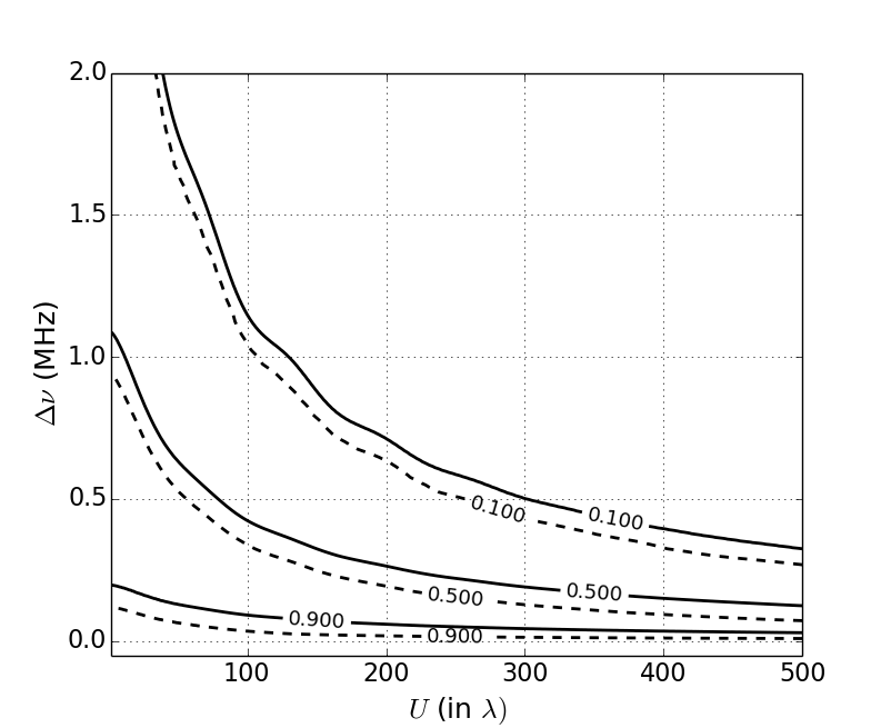
Figure 3: This figure shows how $\Delta\nu$ is varying as a function of U for a given values of frequency decorrelation function ${\kappa}_{U}(\Delta\nu)$ indicated in the figure. Dashed lines show the relation for the scale dependent bias model whereas solid lines are for the linear bias model. As seen in figure 2, we find that the signal remains correlated to larger frequency differences with linear bias. The baryon acoustic oscillations leaves a clear signature in the decorrelation.

Figure 4: The expected visibility correlation $VV^{*}=S_{2}(U,\Delta\nu)$ as a function of U for OWFA. The solid (red) curve shows the expected signal and dashed (black) curve shows the expected noise in the visibility correlation. The solid blue line is for scale independent bias whereas the red line is for scale dependent bias + non-linear evolution of perturbation. In both the plots the red curve sits above the blue curve by $10\%-30\%$ showing that the scale dependent effects are important for calculation of the signal. The noise is calculated for 1000 Hrs of integration. This is shown for signal binned in 9 (left panel)and 5 (right panel)logarithmic bins. We observe that $1\sigma$ detection is possible with $10^{3}$ hrs of integration for the signal in baseline range of $U\sim 20-200$.

Figure 5: Expected visibility correlation $VV^{*}=S_{2}(U,\Delta\nu)$ as a function of U. Solid (red) curve shows expected signal and dashed (blue) curve shows expected noise in visibility correlation. For GMRT and MWA, noise is calculated for 1000 Hrs of integration. Top left panel shows the expected signal for GMRT. Top right panel shows expected signal for MWA. Left bottom panel shows expected signal for SKA-low ($\nu=284$ MHz) corresponding to bin size $\Delta U=5\lambda$ for different integration times. Right bottom panel shows expected signal for SKA-low corresponding to the bin size $\Delta U=10\lambda$.

5 Noise in visibility correlations

We have used the HI power spectrum $P_{HI}(k)$ shown in Figure 1 (blue curve) to compute visibility correlations using the approach described above. We have also estimated the noise level for OWFA and compared it with the expected signal.

The real part of ${\cal N}(U_{n},\nu)$ has rms fluctuation $\sigma$ given by

$$\sigma=\dfrac{\sqrt{2}k_{B}T_{sys}}{\eta A\sqrt{\Delta{\nu}_{c}\Delta t}}$$ (9)

Values of $T_{sys}$, $\eta$ and $A$ used in our calculations are given in Table 1.

As discussed in (Ali & Bharadwaj, 2014), it is possible to avoid the noise contribution ${N}_{2}(U_{n},\Delta\nu)$ in the visibility correlation ${V}_{2}(U_{n},\Delta\nu)$ by correlating only those visibility measurements where the noise is uncorrelated. In this case, for a fixed baseline U we only correlate the visibilities measured by different redundant antenna pairs or the visibilities measured at different time instants. OWFA has a large redundancy in baselines and redundant baselines provide many independent estimates of the visibility correlation $(\Delta V_{2})$ at the same U where each estimate has an independent system noise contribution, but signal is the same. The OWFA is equatorially mounted, hence the projected baseline lengths do not change as the source is tracked. The noise in the visibilities measured with different antenna pairs is uncorrelated. The noise in the visibilities measured at two different time instants is also uncorrelated. Given that the signal decorrelates within $\Delta\nu\simeq 1MHz$, whereas the bandwidth is much larger, the observing bandwidth $B$ also provides several independent estimates of the visibility correlation. Taking all of these into consideration, we get:

$$(\Delta N_{2})^{2}=\left(\dfrac{2{\sigma}^{2}\Delta t}{t_{obs}}\right)^{2}\dfrac{\Delta{\nu}_{0.5}}{N_{P}B}\ \text{and}\ (\Delta S_{2})^{2}=\dfrac{(S_{2})^{2}\Delta{\nu}_{0.5}}{N_{E}B}$$ (10)

where $\Delta S_{2}$ and $\Delta N_{2}$ are cosmic variance and system noise contribution respectively. $\Delta t$ is the the correlator integration time and $t_{obs}$ is the total observation time. $N_{P}$ and $N_{E}$ denote the number of independent estimates of the system noise and the signal respectively in each baseline bin. $\Delta{\nu}_{0.5}$ is the frequency at which signal decorrelates to $0.5$ times the value at $\Delta{\nu}=0$ and $B$ is the frequency bandwidth of the instrument. For more details about the noise calculation please see Bharadwaj & Ali (2005); Datta, Choudhury, & Bharadwaj (2007); Bagla, Khandai, & Datta (2010).

The total error $\Delta V_{2}$ in the residual visibility is

$$\sqrt{(\Delta V_{2})^{2}}=\sqrt{(\Delta S_{2})^{2}+(\Delta N_{2})^{2}}$$ (11)

Detection is possible with $10^{3}$ hrs of integration for the signal in baseline range of $U\sim 20-200$ (Figure 4). We can optimize bin size to improve prospects for detection. We see that detection with significance $2\sigma$ is possible with $10^{3}$ hrs of integration for the signal binned with $5$ logarithmic bins on baseline scale for the baseline range of $U\sim 20-200$ (Figure 4).

We have done a similar analysis for GMRT, MWA and upcoming SKA-low to compare the results for OWFA with these instruments. Figure 5 shows the expected signal and system noise calculated for GMRT, MWA and SKA-low respectively. We find that HI detection is not possible with either GMRT or MWA for $10^{3}$ hrs of integration time without aggressive binning whereas SKA-low can detect HI signal within 200 Hrs of integration (Figure 5 bottom panels).

We have investigated the Signal to Noise Ratio (SNR) for detecting the HI signal under the assumption that it is possible to completely remove the foregrounds. Figure 6 shows the SNR for OWFA as a function of baselines with data binned in $9$ and $5$ logarithmic bins respectively. We see that $>2\sigma$ detection of the signal is possible in the baseline range $20\leq U\leq 200$ in $\sim 2000$ hrs of integration (Figure 6) for data divided in $9$ logarithmic bins and, for $5$ logarithmic bins, $>3\sigma$ detection of the signal is possible in the baseline range $30\leq U\leq 150$ in $\sim 2000$ hrs of integration (Figure 6) and $>5\sigma$ detection in baseline range $50\leq U\leq 130$ in $\sim 3000$ hrs of integration. We observe that optimizing bin size enhances Signal to Noise Ratio which in turn leads to signal detection with better significance levels. Calculations done using the Fisher matrix approach indicate that a $5\sigma$ detection of the HI power spectrum via measurement of the amplitude of the HI power spectrum is possible in $150$ hours (Bharadwaj, Sarkar, & Ali, 2015). In a later work they have shown (Sarkar, Bharadwaj and Ali, 2017) that a measurement of the binned HI power spectrum in the relevant range of scales is possible in $10^{3}$ hours. Thus it is possible to optimize combining signal in different modes well beyond naive binning that we have considered here.

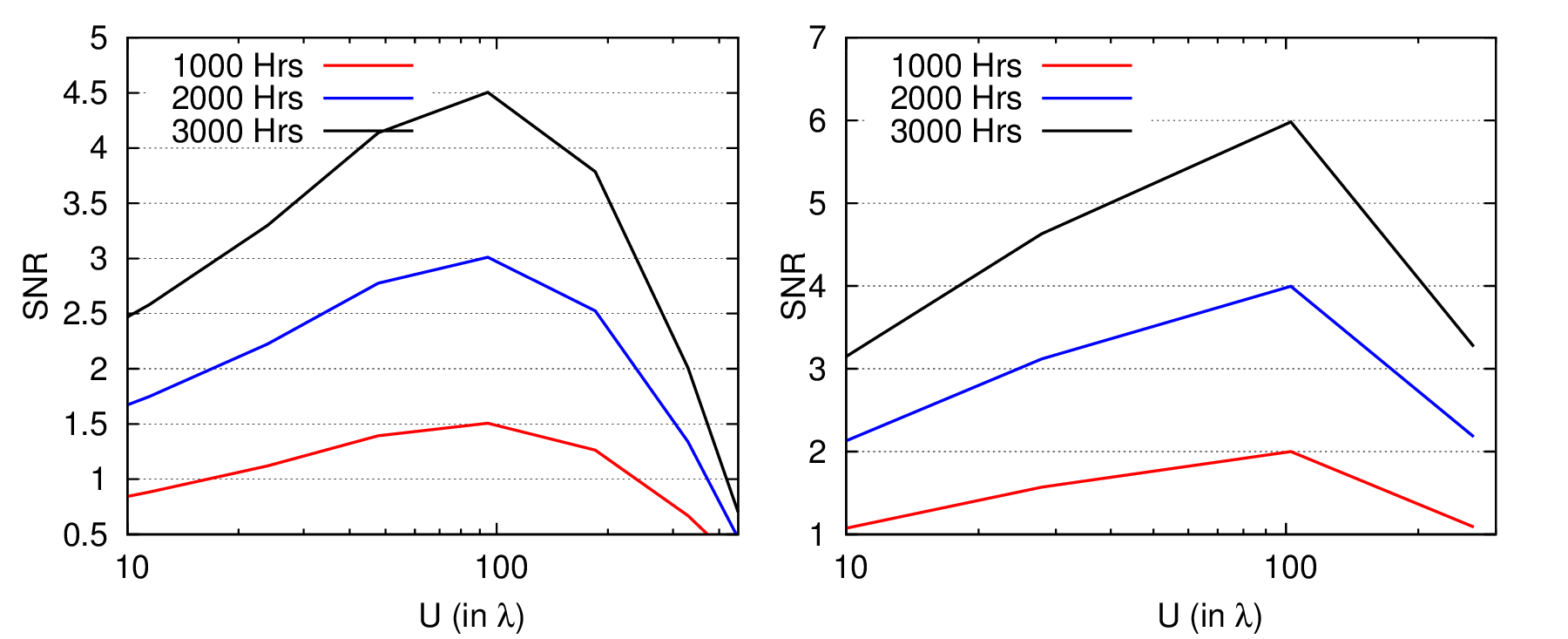
Figure 6: This figure shows the signal to noise ratio (SNR) as function of baseline U with data divided in $9$ logarithmic bins (left panel) and $5$ logarithmic bins (right panel) for different integration times indicated.

6 Summary

We have compared HI detection prospects using upgraded OWFA with GMRT, MWA and SKA-low. OWFA can detect HI signal in about $2000$ Hrs of integration. HI signal detection is not possible with GMRT ($330$ MHz) and MWA ($300$ MHz) for a similar integration. SKA-low ($284$ MHz) can detect HI signal within $200$ Hrs of integration. From the investigation of SNR with different $U$ bin we observe that optimization of $U$ bins can enhance SNR. Significant optimization may be possible using the Fisher matrix approach, and that will be applicable in a similar manner to all instruments apart from subtle variations depending on the relative role of cosmic variance.

We have introduced the concept of a functional form of scale dependent bias defined with respect to the linearly extrapolated dark matter power spectrum. This combines the effects of non-linear evolution and scale dependent bias. This is a useful tool as it allows us to calculate quantities without limiting us to the range of wave modes available in the N-Body simulations that are used to compute bias.

The non-linear evolution of power spectrum and the scale dependent bias enhance the HI power spectrum, but we also see that the signal decorrelates within a shorter frequency range when these factors are taken into account. It is to be noted that we have taken only linear mapping in red-shift space and a direct estimation of the decorrelation function from N-Body simulations is required for a clearer picture.

The prospects for detection of HI distribution at $z\sim 3$ with OWFA are encouraging. Optimizing the bin sizes and using multiple realizations can lead to detection with higher significance level in smaller integration times. Indeed, Fisher matrix based analysis strongly suggests that detection of the amplitude of power spectrum may be possible in a couple of hundred hours while determination of the shape of the power spectrum will require close to $10^{3}$ hours (Bharadwaj, Sarkar, & Ali, 2015; Sarkar, Bharadwaj and Ali, 2017). The comparative analysis suggests that at present OWFA is perhaps the most promising instrument at present for this redshift window, and will continue to be up to the time when SKA-low becomes operational. Given the projected time line for SKA, it is clear that OWFA can make significant contribution in the interim through detection of HI at $z\sim 3$.

In our discussion, we have ignored the role of foregrounds and foreground subtraction. This is likely to impact prospects of detection of the redshifted $21$ cm radiation from intermediate and high redshifts.

The upgraded GMRT (uGMRT) with its wide band receivers will be available soon. This enables observations of a larger comoving volume as compared to the GMRT in a single observation. The expected improvement in sensitivity as a result of wider band is about a factor $3$, and hence with some imaginative co-adding of signal it should be possible to detect the signal in $10^{3}$ hours or so. The uGMRT can play an important role in detection of redshifted $21$ cm radiation from $z\sim 3$. Predictions for uGMRT need to account for the evolution of signal as the wide band encompasses a large range of redshifts.

References

- Ali, Bharadwaj & Chengalur (2008) Ali S. S., Bharadwaj S., Chengalur J. N., 2008, MNRAS, 385, 2166
- Ali & Bharadwaj (2014) Ali S. S., Bharadwaj S., 2014, JApA, 35, 157
- Bagla, Nath, & Padmanabhan (1997) Bagla J. S., Nath B., Padmanabhan T., 1997, MNRAS, 289, 671
- Bagla, Khandai, & Datta (2010) Bagla J. S., Khandai N., Datta K. K., 2010, MNRAS, 407, 567
- Bargur et al. (2011) Bargur G. S., Prasad P., Subrahmanya C. R., Manoharan P. K., Nandagopal D., Dhivya S., 2011, ASInC, 3, 165
- Bharadwaj & Sethi (2001) Bharadwaj S., Sethi S. K., 2001, JApA, 22, 293
- Bharadwaj & Ali (2005) Bharadwaj S., Ali S. S., 2005, MNRAS, 356, 1519
- Bharadwaj, Sethi, & Saini (2009) Bharadwaj S., Sethi S. K., Saini T. D., 2009, PhRvD, 79, 083538
- Bharadwaj, Sarkar, & Ali (2015) Bharadwaj S., Sarkar A. K., Ali S. S., 2015, JApA, 36, 385
- Carilli & Walter (2013) Carilli C. L., Walter F., 2013, ARA&A, 51, 105
- Chang et al. (2008) Chang T.-C., Pen U.-L., Peterson J. B., McDonald P., 2008, PhRvL, 100, 091303
- Chang et al. (2010) Chang T.-C., Pen U.-L., Bandura K., Peterson J. B., 2010, Natur, 466, 463
- Chengalur, Braun, & Wieringa (2001) Chengalur J. N., Braun R., Wieringa M., 2001, A&A, 372, 768
- Datta, Choudhury, & Bharadwaj (2007) Datta K. K., Choudhury T. R., Bharadwaj S., 2007, MNRAS, 378, 119
- Delhaize et al. (2013) Delhaize J., Meyer M. J., Staveley-Smith L., Boyle B. J., 2013, MNRAS, 433, 1398
- Font-Ribera et al. (2012) Font-Ribera A., et al., 2012, JCAP, 11, 59
- Furlanetto, Oh, & Briggs (2006) Furlanetto S. R., Oh S. P., Briggs F. H., 2006, PhR, 433, 181
- Ghosh et al. (2011) Ghosh A., Bharadwaj S., Ali S. S., Chengalur J. N., 2011, MNRAS, 418, 2584
- Ghosh, Koopmans, Chapman & Jelić (2015) Ghosh A., Koopmans L. V. E., Chapman E., Jelić V., 2015, MNRAS, 452, 1587
- Giovanelli & Haynes (2016) Giovanelli R., Haynes M. P., 2016, A&ARv, 24, 1
- Joshi et al. (1988) Joshi M. N., Swarup G., Bagri D. S., Kher R. K., 1988, BASI, 16, 111
- Kaiser (1987) Kaiser N., 1987, MNRAS, 227, 1
- Kanekar, Sethi, & Dwarakanath (2016) Kanekar N., Sethi S., Dwarakanath K. S., 2016, ApJ, 818, L28
- Kapahi et al. (1975) Kapahi V. K., Damle S. H., Balasubramanian V., Swarup G., 1975, Journal of the Institution of Electronics and Telecommunication Engineers, 21, 117
- Lah et al. (2007) Lah P., et al., 2007, MNRAS, 376, 1357
- Liu et al. (2010) Liu A., Tegmark M., Morrison S., Lutomirski A., Zaldarriaga M., 2010, MNRAS, 408, 1029
- Marthi & Chengalur (2014) Marthi V. R., Chengalur J., 2014, MNRAS, 437, 524
- Masui et al. (2013) Masui K. W., Switzer E. R., Banavar N., Bandura K., Blake C., Calin L.-M., Chang T.-C., Chen X., Li Y.-W., Natarajan A., Pen U.-L., Peterson J. B., Shaw J. R., Voytek T. C., 2013, ApJL 763, L20
- Noterdaeme et al. (2012) Noterdaeme P., et al., 2012, A&A, 547, L1
- Padmanabhan, Choudhury, & Refregier (2015) Padmanabhan H., Choudhury T. R., Refregier A., 2015, MNRAS, 447, 3745
- Prasad & Subrahmanya (2011) Prasad P., Subrahmanya C. R., 2011, Experimental Astronomy, 31, 1
- Pritchard & Loeb (2012) Pritchard J. R., Loeb A., 2012, RPPh, 75, 086901
- Purcell & Field (1956) Purcell E. M., Field G. B., 1956, ApJ, 124, 542
- Rhee et al. (2016) Rhee J., Lah P., Chengalur J. N., Briggs F. H., Colless M., 2016, MNRAS, 460, 2675
- Rhee et al. (2013) Rhee J., Zwaan M. A., Briggs F. H., Chengalur J. N., Lah P., Oosterloo T., van der Hulst T., 2013, MNRAS, 435, 2693
- Santos et al. (2015) Santos M., et al., 2015, aska.conf, 19
- Sarkar, Bharadwaj and Ali (2017) Sarkar A. K., Bharadwaj S., Ali S. S. 2017, JApA, This issue.
- Sarma et al. (1975) Sarma N. V. G., Joshi M. N., Bagri D. S., Ananthakrishnan S., 1975, Journal of the Institution of Electronics and Telecommunication Engineers, 21, 110
- Subrahmanya, Manoharan and Chengalur (2014) Subrahmanya C. R., Manoharan P. K. and Chengalur Jayaram, 2014, Proceedings of the Metrewavelength Sky Conference, J. N. Chengalur & Y. Gupta eds.
- Subrahmanya, Manoharan and Chengalur (2017) Subrahmanya C. R., Manoharan P. K. and Chengalur Jayaram, 2017, JApA, This issue.
- Swarup et al. (1971) Swarup G., et al., 1971, NPhS, 230, 185
- Tingay et al. (2013) Tingay S. J., et al., 2013, PASA, 30, 7
- van de Hulst, Raimond, & van Woerden (1957) van de Hulst H. C., Raimond E., van Woerden H., 1957, BAN, 14, 1
- Villaescusa-Navarro et al. (2014) Villaescusa-Navarro F., Viel M., Datta K. K., Choudhury T. R., 2014, JCAP, 9, 050
- Wieringa (1991) Wieringa M., 1991, ASPC, 19, 192
- Wieringa (1992) Wieringa M. H., 1992, ExA, 2, 203
- Wild (1952) Wild J. P., 1952, ApJ, 115, 206
- Wolfe, Gawiser, & Prochaska (2005) Wolfe A. M., Gawiser E., Prochaska J. X., 2005, ARA&A, 43, 861
- Wouthuysen (1952a) Wouthuysen S., 1952a, Phy, 18, 75
- Wouthuysen (1952b) Wouthuysen S. A., 1952b, AJ, 57, 31
- Wyithe & Brown (2010) Wyithe J. S. B., Brown M. J. I., 2010, MNRAS, 404, 876
- Zafar et al. (2013) Zafar T., Péroux C., Popping A., Milliard B., Deharveng J.-M., Frank S., 2013, A&A, 556, A141
- Zaroubi & Hoffman (1996) Zaroubi S., Hoffman Y., 1996, ApJ, 462, 25
- Zaroubi (2013) Zaroubi S., 2013, ASSL, 396, 45
- Zwaan et al. (2005) Zwaan M. A., Meyer M. J., Staveley-Smith L., Webster R. L., 2005, MNRAS, 359, L30
- Zwaan (2000) Zwaan M. A., 2000, PhDT