In Search of an Entity Resolution OASIS:
Optimal Asymptotic Sequential Importance Sampling

Abstract

Entity resolution (ER) presents unique challenges for evaluation methodology. While crowdsourcing platforms acquire ground truth, sound approaches to sampling must drive labelling efforts. In ER, extreme class imbalance between matching and non-matching records can lead to enormous labelling requirements when seeking statistically consistent estimates for rigorous evaluation. This paper addresses this important challenge with the OASIS algorithm: a sampler and F-measure estimator for ER evaluation. OASIS draws samples from a (biased) instrumental distribution, chosen to ensure estimators with optimal asymptotic variance. As new labels are collected OASIS updates this instrumental distribution via a Bayesian latent variable model of the annotator oracle, to quickly focus on unlabelled items providing more information. We prove that resulting estimates of F-measure, precision, recall converge to the true population values. Thorough comparisons of sampling methods on a variety of ER datasets demonstrate significant labelling reductions of up to 83% without loss to estimate accuracy.

1 Introduction

The very circumstances that give rise to entity resolution (ER) systems—lack of shared keys between data sources, noisy/missing features, heterogeneous distributions—explain the critical role of evaluation in the ER pipeline [christen2007quality]. Production systems rarely achieve near-perfect precision and recall due to these many inherent ambiguities, and when they do, even minute increases to error rates can lead to poor user experience [negahban2012scaling], lost business [verykios2000accuracy], or erroneous diagnoses and public health planning [harron2014evaluating]. It is thus vital that ER systems are evaluated in a statistically sound manner so as to capture the true accuracy of entity resolution. This paper addresses this challenge with the development of an algorithm based on adaptive importance sampling, which we call ‘OASIS’.

While crowdsourcing platforms provide inexpensive provisioning of annotations, sampling items for labelling must proceed carefully. A key challenge in ER is the inherent imbalance between matching and non-matching records which can be as high as $1:n$ when matching two sources of $n$ records (e.g., reaching the millions). Researchers leverage several existing practices to evaluate such an ER system: (i) Label samples drawn from all candidate matches uniformly at random (e.g., record pairs in two-source integration): while yielding unbiased estimates, this can take thousands of samples before finding one match-labelled sample, and many tens of thousands of labels before estimates converge. (ii) Balance inefficient passive sampling with cheap crowdsourcing resources: while crowdsourcing facilitates ER evaluation, large nonstationary datasets require constant refresh and can quickly drive costs back up. (iii) Exploit blocking schemes or search facilities to reduce non-match numbers: such filtering injects hidden bias into estimates.

By contrast, OASIS offers a principled alternative to evaluating F-measure, precision, recall—robust measures under imbalance—given an ER system’s set of output similarity scores. OASIS forms an instrumental distribution from which it samples record pairs non-uniformly, minimising the estimator’s asymptotic variance. This instrumental distribution is based on estimates of latent truth due to a simple Bayesian model, and is updated iteratively. By stratifying the pool of record pairs by similarity score, OASIS transfers performance estimates and samples fewer points. By ensuring our sampler may (with non-zero probability) sample any stratum, we manage the explore-exploit trade-off, admitting guarantees of statistical consistency: our estimates of F-measure, precision, recall converge to the true population parameters with high probability.

The unique characteristics of OASIS together yield a rigorous approach to ER evaluation that can use orders-of-magnitude fewer labels. This is borne out in thorough comparisons of baselines across six datasets of varying sizes and class imbalance (up to over 1:3000).

Contributions. 1) The novel OASIS algorithm for efficient evaluation of ER based on adaptive importance sampling. This algorithm has been released as an open-source Python package at https://git.io/OASIS ;
2) Theoretical guarantee that OASIS yields statistically consistent estimates, made challenging by the non-independence of the samples and the non-linearity of the F-measure; and
3) A comprehensive experimental comparison of OASIS with existing state-of-the-art algorithms demonstrating superior performance e.g., 83% reduction in labelling requirements under a class imbalance of 1:3000.

2 Background

Motivated by the challenges of accurate but efficient evaluation of ER, we begin by reviewing the key features of ER.

2.1 Entity resolution

Definition 1 (ER problem)

Let $\mathcal{D}_{1}$ and $\mathcal{D}_{2}$ denote two databases, each containing a finite number of records $n_{1},n_{2}$ representing underlying entities; and let fixed, unknown relation $\mathcal{R}\subseteq\mathcal{D}_{1}\times\mathcal{D}_{2}$ describe the matching records across the databases, i.e., pairs of records representing the same entity. The entity resolution problem is to approximate $\mathcal{R}$ with a predicted relation $\hat{\mathcal{R}}\subseteq\mathcal{D}_{1}\times\mathcal{D}_{2}$.

Remark 1

For simplicity we focus on two-source ER, however our algorithms and theoretical results apply equally well to multi-source ER on relations over larger product spaces, and deduplicating a single source.

An abundant literature describes the typical ER pipeline: preparation amortising record canonicalisation; blocking for reducing pair comparisons through a linear database scan; scoring, the most expensive stage, in which pair attributes are compared and summarised in similarity scores; and matching where sufficiently high-scoring pairs are used to construct $\hat{\mathcal{R}}$. Further normalisation pre- or post-linkage such as schema matching or record merging, while non-core, are important also. We refer the interested reader to review articles [winkler_overview_2006, christen_data_2012, getoor_entity_2013] and the references therein.

2.1.1 Similarity scores

ER is often cast as a binary classification problem on the set of record pairs $\mathcal{Z}=\mathcal{D}_{1}\times\mathcal{D}_{2}$. A pair $z\in\mathcal{Z}$ has true Boolean label 1 if a “match”, that is $z\in\mathcal{R}$, and label 0 if a “non-match”, that is $z\notin\mathcal{R}$. In this work, we leverage the similarity scores produced in typical ER pipelines:

Definition 2

A similarity score $s(z)\in\mathbb{R}$ quantifies the level of similarity that a given pair $z\in\mathcal{Z}$ exhibits, i.e., the predicted confidence of a match.

Similarity scores originate from a variety of sources. The scoring phase of typical ER pipelines combine attribute-level dis/similarity measures e.g., edit distance, Jaccard distance, absolute deviation, etc., into similarity scores. The combination itself is often produced by hand-coded rules or supervised classification, fit to a training set of known non/matches. Unlike in evaluation, data used for training need not be representative: heuristically-compiled training sets may be used when learning discriminative models. Any confidence-based classifier, e.g., the support vector machine, or probabilistic classifier, e.g., logistic regression or probability trees, produces legitimate similarity scores. Scores from probabilistic classifiers may or may not be calibrated:

Definition 3

A scoring function $s(\cdot)$ is calibrated if, of all the record pairs mapping to $s(z)=\rho\in[0,1]$, approximately $100\times\rho$ percent are truly matching. For example, 60% of pairs with a score of 0.6 should be matches.

2.2 Evaluation measures for ER

All ER evaluation methods produce statistics that summarise the types of errors made in approximating $\mathcal{R}$ with $\hat{\mathcal{R}}$. Arguably the most popular among these statistics is the pairwise F-measure which we focus on in this work. The F-measure is particularly well suited to ER, unlike accuracy for example, as its invariance to true negatives makes it more robust to class imbalance. The F-measure is a weighted harmonic mean of precision and recall; and in terms of Type I and Type II errors, the statistic on $T$ labels is

$$F_{\alpha,T} = \frac{\mathrm{TP}}{\alpha(\mathrm{TP}+\mathrm{FP})+(1-\alpha)(\mathrm{TP}+\mathrm{FN})}\enspace,$$ (1)

where $\alpha\in[0,1]$ is a weight parameter; TP, FP, FN are true positive, false positive, false negative counts respectively.

$$\mathrm{TP}=\sum_{t=1}^{T}\ell_{t}\hat{\ell}_{t}\enspace,\enspace\mathrm{FP}=\sum_{t=1}^{T}(1-\ell_{t})\hat{\ell}_{t}\enspace,\enspace\mathrm{FN}=\sum_{t=1}^{T}\ell_{t}(1-\hat{\ell}_{t})\enspace,$$

where $z_{1},\ldots,z_{T}\sim p$ are query pairs sampled i.i.d from some underlying distribution $p$ of interest on $\mathcal{Z}$ such as the uniform distribution; the $\ell_{t}$ denote ground truth labels recording (possibly noisy) membership of $z_{t}$ within $\mathcal{R}$; and $\hat{\ell}_{t}$ indicates $z_{t}\in\hat{\mathcal{R}}$. When $\alpha=1$, $F_{\alpha,T}$ reduces to precision, $\alpha=0$ produces recall, and $\alpha=1/2$ yields the balanced F-measure, with equal importance on precision and recall.

Our goal will be to estimate the asymptotic limit of $F_{\alpha,T}$ as label budget $T\to\infty$. For finite pools $\mathcal{Z}$ this corresponds to labelling of all record pairs with sufficient repetition to account for (any) noise in the ground truth labels $\ell_{t}$.

Remark 2

The pairwise F-measure is termed “pairwise” to highlight the application of the measure to record pairs. Pairwise measures work well when there are only a few records across the databases which correspond to a particular entity. In such cases one should not use accuracy, due to significant class imbalance (cf. Section 3). For cases where most entities have many matching records, one may leverage transitivity constraints while looking to cluster-based measures for evaluation [menestrina_evaluating_2010]. See [barnes_practioners_2015] for a summary on evaluation.

3 Problem formulation

Suppose we are faced with the task of evaluating an ER system as described in the previous section. Given that we do not know $\mathcal{R}$, how can we efficiently leverage labelling resources to estimate the pairwise F-measure?

Definition 4 (Efficient evaluation problem)

Consider evaluating a predicted ER $\hat{\mathcal{R}}\subseteq\mathcal{Z}=\mathcal{D}_{1}\times\mathcal{D}_{2}$, equivalently represented by predicted labels $\hat{\ell}(z)=\mathbf{1}\big{[}z\in\hat{\mathcal{R}}\big{]}$ for $z\in\mathcal{Z}$. We are given access to:

• a pool $P\subseteq\mathcal{Z}$ of record pairs, e.g., $P=\mathcal{Z}$;

• a similarity scoring function $s:\mathcal{Z}\to\mathbb{R}$; and

• a randomised labelling $\mathtt{Oracle}:\mathcal{Z}\to\{0,1\}$, which returns labels $\ell(z)\sim\mathtt{Oracle}(z)$ indicating membership in $\mathcal{R}$. The oracle’s response distribution is parametrised by oracle probabilities $p(1|z)=\Pr[\mathtt{Oracle}(z)=1]$.

With this setup, the efficient evaluation problem is to devise an estimation procedure for $F_{\alpha}$, which samples record pairs $z_{1},\ldots,z_{T}\in P$ and makes use of the corresponding labels provided by the oracle. We adopt integer index notation on $\hat{\ell},\ell$ and $s$ to denote their values at the $t$-th query; e.g., $\hat{\ell}_{t}=\hat{\ell}(z_{t})$ for query $z_{t}$.

Solutions should produce estimates $\hat{F}_{\alpha,T}$ exhibiting:

1. consistency: convergence in probability to the true value $F_{\alpha}$ on pool $P$ with respect to underlying distribution $p$

   $$F_{\alpha}=\lim_{T\to\infty}F_{\alpha,T}\enspace;\enspace\mbox{and}\vspace{-1ex}$$ (2)

2. minimal variance: vary minimally about $F_{\alpha}$.

In other words, solutions should produce precise estimates whilst minimising queries to the oracle, since it is assumed that queries come at a high cost. Computational efficiency of the estimation procedure is not a direct concern, so long as the response time of the oracle dominates (typically of order seconds in a crowdsourced setting).

ER poses unique challenges for efficient evaluation.

Challenge: Extreme class imbalance. The inherent class imbalance in ER presents a challenge for estimation of F-measure. For deduped databases $\mathcal{D}_{1},\mathcal{D}_{2}$, the minimum possible class imbalance occurs when both DBs contain $n$ records and there is a matching record in $\mathcal{D}_{1}$ for every record in $\mathcal{D}_{2}$. In this case, the class imbalance ratio (ratio of non-matches to matches) is $n-1$. This is problematic for passive (uniform i.i.d.) sampling even for modest-sized databases, since $\mathcal{O}(n)$ expected pairs would be sampled for every match found. As $F_{\alpha}$ depends only on matches (both predicted and true), many queries to the oracle would be wasted on labels that don’t contribute. The problem becomes one of searching for an oasis within a desert when $n\sim 10^{6}$ or more.

Approach: Biased sampling. One response to class imbalance is biased sampling, that is, sampling from a population (or space more generally) in a way that systematically differs from the underlying distribution [rubinstein_simulation_2007, Chapter 5]. Biased sampling methods have found broad application in areas as diverse as survey methodology, Monte Carlo simulations, and active learning, to name a few. They work by leveraging known information about the system—here the similarity scores and the pool of record pairs—to obtain more precise estimates using fewer samples. One of the most effective biased sampling methods is importance sampling (IS), which we illustrate below:

Example

Consider a random variable $X$ with probability density $p(x)$ and consider the estimation of parameter $\theta=\operatorname{E}[f(X)]$. The standard (passive) approach draws an i.i.d. sample from $p$ and uses the Monte Carlo estimator $\hat{\theta}=\frac{1}{T}\sum_{i=1}^{T}f(x_{i})$. Importance sampling, by contrast, draws from an instrumental distribution denoted by $q$. Even though the sample from $q$ is biased (i.e. not drawn from $p$), an unbiased estimate of $\theta$ can be obtained by using the bias-corrected estimator $\hat{\theta}^{\mathrm{IS}}=\frac{1}{T}\sum_{i=1}^{T}\frac{p(x_{i})}{q(x_{i})}f(x_{i})$.

An important consideration when conducting IS is the choice of instrumental distribution, $q$. If $q$ is poorly selected, the resulting estimator may perform worse than passive sampling. If on the other hand, $q$ is selected judiciously, so that it concentrates on the “important” values of $X$, significant efficiency dividends will follow.

4 A New Algorithm: OASIS

This section develops our new algorithm for evaluating ER—Optimal Asymptotic Sequential Importance Sampling (OASIS). In designing an adaptive/sequential importance sampler (AIS), we proceed in two stages: (i) choosing an appropriate instrumental distribution to optimise asymptotic variance of the estimator, see Section 4.1; and (ii) deriving an appropriate update rule and initialisation process for the instrumental distribution, now restricted to score strata, see Sections 4.2 and 4.3. Section 4.4 brings all of the components of OASIS together, presenting the algorithm in its entirety. Section 5 presents a thorough theoretical analysis of OASIS.

4.1 Selecting the instrumental distribution

We begin by defining an estimator for the F-measure which corrects for the bias of AIS. It is based on the standard estimator of Eqn. (1), with the addition of importance weights.

Definition 5

Let $\{x_{t}=(z_{t},\ell_{t})\}_{t=1}^{T}$ be a sequence of record pairs and labels, where the $t$-th record pair in the sequence is drawn from pool $P$ according to an instrumental distribution $q_{t}$, which may depend on the previously sampled items $\bm{x}_{1:t-1}=\{x_{1},\ldots,x_{t-1}\}$ and labels $\ell_{t}\sim\mathtt{Oracle}(z_{t})$. Then the AIS estimator for the F-measure is given by

$$\hat{F}_{\alpha}^{\mathrm{AIS}}=\frac{\sum_{t=1}^{T}w_{t}\ell_{t}\hat{\ell}_{t}}{\alpha\sum_{t=1}^{T}w_{t}\hat{\ell}_{t}+(1-\alpha)\sum_{t=1}^{T}w_{t}\ell_{t}}\enspace,$$ (3)

where $w_{t}=p(z_{t})/q_{t}(z_{t})$ is the importance weight associated with the $t$-th item, and $p$ denotes any underlying distribution on the record pairs from which the target $F_{\alpha}$ is defined.

This definition assumes that the record pairs are drawn from an, as yet, unspecified sequence of instrumental distributions $\{q_{t}\}_{t=1}^{T}$. It is important that these instrumental distributions are selected carefully, so as to maximise the sampling efficiency. Later, we justify the choice of $\hat{F}_{\alpha}^{\mathrm{AIS}}$ by proving that it is consistent for $F_{\alpha}$ (cf. Theorem 5.3).

Remark 3

In ER we take: $P\subseteq\mathcal{Z}$ typically a DB product space $\mathcal{D}_{1}\times\mathcal{D}_{2}$ which is finite (but possibly massive); and the $p$ through which $F_{\alpha,T}$ is most naturally defined is the uniform distribution on $P$ i.e., placing uniform mass $1/N$ where $N=|P|$. However OASIS and its analysis actually hold more generally: pools $P$ of instances that could be uncountably infinite in size; and arbitrary marginal distributions $p$ on $P$.

4.1.1 Variance minimisation

A common approach for instrumental distribution design is based on the principle of variance minimisation [rubinstein_simulation_2007]. In the ideal case, a single instrumental distribution (for all $t$) is selected that minimises the variance of the estimator:

$$q^{\star}\in\arg\underset{q}{\min}\ \mathrm{Var}(\hat{F}_{\alpha}^{\mathrm{AIS}}[q])\enspace.$$ (4)

This optimisation problem is difficult to solve analytically, in part due to the intractability of the variance term. However, by replacing variance with the asymptotic variance (taking $T\to\infty$), a solution is obtained as

$$\begin{split}q^{\star}(z)&\propto p(z)\left[(1-\alpha)(1-\hat{\ell}(z))F_{\alpha}\sqrt{p(1|z)}\right.\\ &\left.\;\;\;\;+\hat{\ell}(z)\sqrt{\alpha^{2}F_{\alpha}^{2}(1-p(1|z))+(1-F_{\alpha})^{2}p(1|z)}\right],\end{split}$$ (5)

where $p(z)$ is the underlying distribution on $P$ (see Remark 3) and $p(1|z)$ is the oracle probability (see Definition 4). The proof of this result is given in [sawade_active_2010]. We call $q^{\star}(z)$ the asymptotically optimal instrumental distribution, owing to its relationship with asymptotic minimal variance.

4.1.2 Motivation for adaptive sampling

Close examination of (5) reveals that the asymptotically optimal instrumental distribution depends on the true F-measure $F_{\alpha}$ and true oracle probabilities $p(1|z)$, both of which are unknown a priori. This implies that an adaptive procedure is well-suited to this problem: we estimate $q^{\star}$ at iteration $t$ using estimates of $F_{\alpha}$ and $p(1|z)$, which themselves are based on the previously sampled record pairs and labels $\bm{x}_{1:t-1}$. As the sampling progresses and labels are collected, the estimates of $F_{\alpha}$ and $p(1|z)$ should approach their true values, and $q_{t}^{\star}$ should in turn approach $q^{\star}$.

In order to implement this adaptive procedure, we must devise a way of iteratively estimating $F_{\alpha}$ and $p(1|z)$. There is a natural approach for $F_{\alpha}$: we simply use $\hat{F}_{\alpha}^{\mathrm{AIS}}$ at the current iteration. However, the oracle probabilities present more of a difficulty. We outline one approach in Section 4.2.

4.1.3 Exploration vs. exploitation

In the subsequent analysis of OASIS (cf. Section 5), we show that the asymptotically optimal instrumental distribution given in Eqn. (5) does not guarantee consistency (convergence in probability). This is because it permits zero weight to be placed on some items, meaning that parts of the pool may never be explored. Consequently, we propose to replace $q^{\star}$ by an $\varepsilon$-greedy distribution

$$q(z)=\varepsilon\cdot p(z)+(1-\varepsilon)\cdot q^{\star}(z)\enspace,$$ (6)

where $0<\varepsilon\leq 1$. For $\varepsilon$ close to 0, the sampling approaches optimality (it exploits), whereas for $\varepsilon$ close to 1, the sampling approaches passivity (it explores). This bears resemblance to explore-exploit trade-offs commonly encountered in online decision making (e.g., multi-armed bandits) [cesa-bianchi_prediction_2006].

4.2 Estimating the oracle probabilities

In this section, we propose an iterative method for estimating the oracle probabilities, which are required for the estimation of $q^{\star}$. Our proposed method brings together two key concepts: stratification and a Bayesian generative model of the label distribution.

4.2.1 Stratification

Stratification is a commonly used technique in statistics that involves dividing a population into homogeneous subgroups (called strata) [cochran_sampling_1977]. Often the process of creating the strata is achieved by binning according to a variable, or partitioning according to a set of rules. Our use of stratification is somewhat atypical, in that we are not using it to estimate a population parameter, but rather as a parameter reduction technique. Specifically, we aim to map the set of oracle probabilities $\{p(1|z):z\in P\}$ (of size $N=|P|$ in ER) to a smaller set of parameters of size $K$, essentially one per stratum.

Parameter reduction. Consider a partitioning of record pair pool $P$ into $K$ disjoint strata $\{P_{1},\ldots,P_{K}\}$, such that the pairs in a stratum share approximately the same values of $p(1|z)$. If this ideal condition is satisfied, then our work in estimating the set of probabilities $\{p(1|z):z\in P\}$ is significantly reduced, because information gained about a particular pair $z\in P_{k}$ is immediately transferable to the other pairs in $P_{k}$. As a result, we can effectively replace the set of probabilities $\{p(1|z):z\in P_{k}\}$ for the record pairs in $P_{k}$, by a single probability $p(1|P_{k})$.

Relaxing the homogeneity condition. In reality, we don’t know which record pairs in $P$ (if any) have roughly the same values of $p(1|z)$. Fortunately, it turns out that this condition does not need to be satisfied too strictly in order to be useful. Previous work [bennett_online_2010, druck_toward_2011] has demonstrated that the homogeneity condition can be satisfied in an approximate sense by using similarity scores as a proxy for true oracle probabilities. In other words, we regard a stratum to be approximately homogeneous if the pairs it contains have roughly the same similarity scores. The more this proxy holds true, the more efficient OASIS becomes in practice; however critically, our guarantees hold true regardless.

Stratification method. In order to stratify the record pairs in $P$ according to their similarity scores, we shall use the cumulative $\sqrt{F}$ (CSF) method, originally proposed in [dalenius_minimum_1959] and previously used in the present context in [druck_toward_2011]. The CSF method has a strong theoretical grounding, in that it aims to achieve minimal intra-stratum variance in the scores.

Algorithm 1 Cumulative $\sqrt{F}$ (CSF) stratification [dalenius_minimum_1959]

1:

$P$	pool of record pairs
$s$	similarity score function $:P\to\mathbb{R}$
$\tilde{K}$	desired number of strata
$M$	number of bins (for estimating score dist.)

2:strata $P_{1},\ldots,P_{K}$ (not guaranteed $K=\tilde{K}$)

3:Pool scores: $S\leftarrow\{s(z)|z\in P\}$

4: Distribution of scores ($F$) using $M$ bins: $\texttt{counts},\texttt{score\_bins}\leftarrow\operatorname{histogram}(S,\mathrm{bins}=M)$

5:Cum. dist. of $\sqrt{F}$: $\texttt{csf}\leftarrow\big{[}\sum_{i=1}^{m}\sqrt{\texttt{counts}[i]}\,\big{]}_{m=1:M}$

6:Bin width on cum. $\sqrt{F}$ scale: $w\leftarrow\texttt{csf}[M]/\tilde{K}$

7:for $k\in\{1,\ldots,\tilde{K}+1\}$ do

8:     Bins on cum. $\sqrt{F}$ scale: $\texttt{csf\_bins}[k]\leftarrow(k-1)w$

9:end for

10:$K\leftarrow 1$

11:for $j\in\{1,\ldots,M\}$ do

12:     if $K=\tilde{K}$ or $j=M$ then

13:         Append $\texttt{score\_bins}[\tilde{K}]$ to new_bins

14:         break

15:     end if

16:     if $\texttt{csf}[j]\geq\texttt{csf\_bin}[K]$ then

17:         Append $\texttt{score\_bins}[j]$ to new_bins

18:         $K\leftarrow K+1$

19:     end if

20:end for

21:Allocate record pairs $P$ to strata $P_{1},\ldots,P_{K}$ based on new_bins (remove any empty strata, updating $K$)

22:return $P_{1},\ldots,P_{K}$

For completeness, we have included an implementation of the method in Algorithm 1. It proceeds by constructing an empirical estimate of the cumulative square root of the distribution of scores (lines 2–3). Then the strata are defined as equal-width bins on the CSF scale (lines 4–7). Finally, the bins are mapped from the CSF scale to the score scale (lines 8–18), so that the scores (record pairs) may be binned in the usual way (line 19). We note that any stratification method could be used in place of the CSF method (cf. e.g., the equal size method described in [druck_toward_2011]).

Selecting the number of strata. The number of strata $K$ represents a trade-off: For large $K$, estimates of the oracle probabilities enjoy finer granularity and can better approach their true values; however large $K$ leads to more parameters and hence more labels required for convergence of estimates.

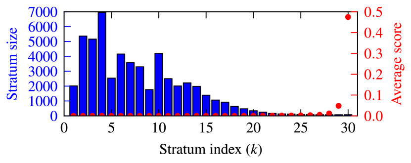
Figure 1: Size and mean score of the CSF strata for the Abt-Buy pool, using calibrated (probabilistic) scores.

In practice for ER evaluation, we find that the there is often a “natural” range of $K$ for the CSF method. The example in Figure 1 shows that we typically construct very large strata with low similarity scores, and very small strata with high similarity scores: a form of heavy-tailed distribution due to the extreme class imbalance. If $K$ is set too large, then we immediately discover the strata corresponding to the higher similarity scores become too small (they may contain only 1 or 2 record pairs). We find a range of $K$ from roughly 30–60 to work well for most datasets considered in Section 6.

4.2.2 A Bayesian generative model

Having partitioned the record pairs in $P$ into $K$ strata $\{P_{1},\ldots,P_{K}\}$, our goal is to estimate $p(1|P_{k})$ (for all $k$) using the collected $\mathtt{Oracle}$ labels. For notational convenience, we denote the true value of $p(1|P_{k})$ by $\pi_{k}$ and a corresponding estimate by $\hat{\pi}_{k}$. We shall adopt a generative model for observed labels which regards $\pi_{k}$ as a latent variable.

Model of a stratum. Consider a label $\ell$ received from the oracle for a record pair in $P_{k}$. We assume that the label is generated from a Bernoulli distribution with probability $\pi_{k}$ of being a match (binary label ‘1’), i.e.,

$$\ell\sim\mathrm{Bernoulli}(\pi_{k})\enspace.$$ (7)

Since the Bernoulli distribution is conjugate to the beta distribution, we adopt a beta prior for $\pi_{k}$:

$$\pi_{k}\sim\mathrm{Beta}(\gamma_{0,k}^{(0)},\gamma_{1,k}^{(0)})\enspace,$$ (8)

where $\gamma_{0,k}^{(0)}$ and $\gamma_{1,k}^{(0)}$ are the prior hyperparameters. We describe how to choose the prior hyperparameters in Sections 4.3 and 4.4.

Joint model of strata. To model each stratum independently but not identically—we do not transfer information across strata but grant each a prior—we factor the joint prior distribution as a product of the marginal $K$ priors. We collect the $\pi_{k}$’s into a vector $\bm{\pi}=[\pi_{1},\pi_{2},\ldots,\pi_{K}]$ and the prior hyperparameters into a $2\times K$ matrix:

$$\bm{\Gamma}^{(0)}=\begin{bmatrix}\gamma_{0,1}^{(0)}&\gamma_{0,2}^{(0)}&\cdots&\gamma_{0,K}^{(0)}\\ \gamma_{1,1}^{(0)}&\gamma_{1,2}^{(0)}&\cdots&\gamma_{1,K}^{(0)}\end{bmatrix}\enspace.$$ (9)

The posterior distribution of $\bm{\pi}$, given the labels received from the oracle up to iteration $t$, is a product of the $K$ corresponding independent beta posterior distributions. Continuing with the previous notation, we store the posterior hyperparameters at iteration $t$ in a matrix $\bm{\Gamma}^{{(t)}}$.

Iterative posterior updates. To obtain a new estimate of $\bm{\pi}$ per iteration, we iteratively update the posterior hyperparameters upon arrival of $\mathtt{Oracle}$ label observations $\ell_{t}$. Suppose label $\ell_{t}$ is observed as a result of querying with a record pair from stratum $P_{k^{\star}}$. Then the update involves:

$$\begin{split}\text{copy old values}&:\quad\bm{\Gamma}^{(t)}\leftarrow\bm{\Gamma}^{(t-1)}\\ \text{if }\ell_{t}=1&:\quad\gamma_{0,k^{\star}}^{(t)}\mathrel{{+}{=}}1\\ \text{if }\ell_{t}=0&:\quad\gamma_{1,k^{\star}}^{(t)}\mathrel{{+}{=}}1\end{split}$$ (10)

A point estimate of $\bm{\pi}$ can be obtained at iteration $t$ via the posterior mean

$$\hat{\bm{\pi}}^{(t)}=\operatorname{E}[\bm{\pi}|\ell_{1},\ldots,\ell_{t}]=\frac{\bm{\Gamma}_{0,:}^{(t)}}{\bm{\Gamma}_{0,:}^{(t)}+\bm{\Gamma}_{1,:}^{(t)}}\enspace.$$ (11)

Here the notation $\bm{\Gamma}_{i,:}^{(t)}$ represents the $i$-th row of matrix $\bm{\Gamma}^{(t)}$, and the division is carried out element-wise.

Remark 4

As a practical modification to speed up convergence of $\hat{\bm{\pi}}$, we can decrease our reliance on the prior as labels are received. For each column $\bm{\Gamma}_{:,k}^{(0)}$ we can retroactively multiply by a factor $1/n_{k}$ where $n_{k}$ is the number of labels sampled from $P_{k}$ thus far. Anecdotally we also observe that this improves robustness to misspecified priors.

4.2.3 Stratified instrumental distribution

Since the estimation method for the oracle probabilities produces estimates over the strata, rather than for individual pairs in the pool, it is appropriate to estimate the instrumental distribution in the same way. Akin to the mapping from $p(1|z)$ to $\bm{\pi}$, we therefore propose to map $q(z)$ to a vector $\bm{v}=[v_{1},\ldots,v_{K}]$ based on our Bayesian stratified model estimates instead of (unknowable) population parameters. Adapting Eqn. (5), the stratified asymptotically optimal instrumental distribution $\bm{v}^{\star}$ is defined at iteration $t$ as

$$\begin{split}v_{k}^{\star(t)}&\propto\omega_{k}\left[(1-\alpha)(1-\lambda_{k})\hat{F}_{\alpha}^{(t-1)}\sqrt{\hat{\pi}_{k}^{(t-1)}}\right.\\ &\left.{}+\lambda_{k}\sqrt{(\alpha\hat{F}_{\alpha}^{(t-1)})^{2}(1-\hat{\pi}_{k}^{(t-1)})+(1-\hat{F}_{\alpha}^{(t-1)})^{2}\hat{\pi}_{k}^{(t-1)}}\right],\end{split}$$

where $\omega_{k}=|P_{k}|/N$ is the weight associated with $P_{k}$ and $\lambda_{k}=\frac{1}{\left|P_{k}\right|}\sum_{i\in P_{k}}\hat{\ell}_{i}$ is the mean prediction in $P_{k}$. It follows that the $\varepsilon$-greedy distribution at iteration $t$ is given by

$$v_{k}^{(t)}=\varepsilon\cdot\omega_{k}+(1-\varepsilon)\cdot v_{k}^{\star(t)}\enspace.$$ (12)

Having adopted a stratified representation for the instrumental distribution, sampling a record pair is now a two-step process. First a stratum index is drawn from $\{1,\ldots,K\}$ according to $\bm{v}$. Then a record pair is drawn uniformly at random from the resulting stratum.

4.3 Initialisation

OASIS requires a set of prior hyperparameters $\bm{\Gamma}^{(0)}$ and a guess for the F-measure $\hat{F}_{\alpha}^{(0)}$ for initialisation purposes. We elect to set these quantities based on the information contained within the similarity scores. Our approach depends centrally on a guess for the oracle probabilities $\hat{\bm{\pi}}^{(0)}$, in that once $\hat{\bm{\pi}}^{(0)}$ is available, the values of $\bm{\Gamma}^{(0)}$ and $\hat{F}_{\alpha}^{(0)}$ immediately follow. The details of the initialisation are contained in Algorithm 2, with further explanation given below.

Oracle probabilities (lines 2–5). A reasonable guess for $\bm{\pi}$ can be obtained by taking the mean of the similarity scores in each stratum. If the scores are not probabilities, they should be mapped to the $[0,1]$ interval. This can be achieved by applying the logistic function.

F-measure (lines 6 & 8). The calculation of $\hat{F}_{\alpha}^{(0)}$ depends on the guess for $\bm{\pi}$ described above and the mean prediction per stratum $\bm{\lambda}$. Breaking down the calculation term-by-term, one begins by estimating the probability of finding a true positive in $P_{k}$ as $\hat{\pi}_{k}^{(0)}\lambda_{k}$, so that the total number of true positives may be approximated by $\sum_{k=1}^{K}|P_{k}|\hat{\pi}_{k}^{(0)}\lambda_{k}$. Similarly, the total number of actual positives (TP + FN) may be approximated by $\sum_{k=1}^{K}|P_{k}|\hat{\pi}_{k}^{(0)}$. The total number of predicted positives (TP + FP) is known exactly and can be written in terms of $\bm{\lambda}$ as $\sum_{k=1}^{K}|P_{k}|\lambda_{k}$. Using these estimates in Eqn. (2) yields the guess for $\hat{F}_{\alpha}^{(0)}$ in line 8.

Prior hyperparameters. We also set $\bm{\Gamma}^{(0)}$ based on $\hat{\bm{\pi}}^{(0)}$

$$\bm{\Gamma}^{(0)}=\eta\begin{bmatrix}\hat{\bm{\pi}}^{(0)}\\ 1-\hat{\bm{\pi}}^{(0)}\end{bmatrix}\enspace.$$

Here $\eta>0$ is an adjustable parameter that controls the strength of the prior. For ease of presentation, this step is included in Algorithm 3 (line 1) rather than Algorithm 2.

Algorithm 2 Initialisation of Bayesian model

1:

$0\leq\alpha\leq 1$	F-measure weight
$P$	pool of record pairs
$\hat{\mathcal{R}}$	predicted ER
$s$	similarity score function $:P\to\mathbb{R}$
$\tau$	$\mathbb{R}$-valued score threshold (optional)
$\{P_{k}\}_{k=1}^{K}$	stratum allocations

2:

$\hat{F}_{\alpha}^{(0)}$	initial F-measure
$\hat{\bm{\pi}}^{(0)}$	prior hyperparameters

3:for $k\in\{1,\ldots,K\}$ do

4:     Mean score per stratum: $\hat{\pi}_{k}^{(0)}\leftarrow\frac{1}{\left|P_{k}\right|}\sum_{z\in P_{k}}s(z)$

5:     if scores are not probabilities in $[0,1]$ then

6:         Transform: $\hat{\pi}_{k}^{(0)}\leftarrow\mathrm{logit}(\hat{\pi}_{k}^{(0)}-\tau)$

7:     end if

8:     Mean pred. per stratum: $\mathbf{\lambda}_{k}\leftarrow\frac{1}{\left|P_{k}\right|}\sum_{z\in P_{k}}\hat{\ell}_{z}$

9:end for

10:$\hat{F}_{\alpha}^{(0)}\leftarrow\frac{\sum_{k=1}^{K}\left|P_{k}\right|\pi_{0,k}\lambda_{k}}{\alpha\sum_{k=1}^{K}\left|P_{k}\right|\lambda_{k}+(1-\alpha)\sum_{k=1}^{K}\left|P_{k}\right|\pi_{0,k}}$

11:return $\hat{F}_{\alpha}^{(0)}$, $\hat{\bm{\pi}}^{(0)}$

4.4 Bringing everything together

Having introduced all of the components of OASIS, we are now ready to explain how they fit together. Recall that the evaluation process begins with three main inputs: the pool of record pairs $P$, similarity scores $s(\cdot)$, and predicted ER $\hat{\mathcal{R}}$. A summary of the main steps involved is as follows:

1. Generate a set of strata $P_{1},\ldots,P_{K}$ partitioning $P$ using the CSF method (Algorithm 1).

2. Generate initial estimates using the strata, $\hat{\mathcal{R}}$ and $s(\cdot)$ (Algorithm 2).

3. Conduct AIS to estimate $F_{\alpha}$ (Algorithm 3).

Summary of Algorithm 3. At each iteration $t$: sample a stratum according to $\bm{v}^{(t)}$, then a record pair within that stratum uniformly at random. Query $\mathtt{Oracle}$ for a label of the record pair. Use the observed label (and the predicted label) to update the oracle probabilities (using Eqn. 10) and the F-measure estimate (using Eqn. 3). Stop after $T$ iterations and return the final estimate $\hat{F}_{\alpha}^{(T)}$.

Algorithm 3 OASIS for estimation of the F-measure

1:

$T>0$	number of iterations
$0\leq\alpha\leq 1$	F-measure weight
$0<\varepsilon\leq 1$	greediness parameter
$\eta>0$	prior strength parameter
$\hat{F}_{\alpha}^{(0)}$	initial guess for F-measure
$\hat{\bm{\pi}}^{(0)}$	initial guess for pos. probabilities
$\hat{\mathcal{R}}$	predicted ER
$\{P_{k}\}_{k=1}^{K}$	stratum allocations
Oracle	randomised (noisy) true labels

2:

$\hat{F}_{\alpha}^{(T)}$

F-measure estimate

3:$\bm{\Gamma}\leftarrow\eta\begin{bmatrix}\hat{\bm{\pi}}^{(0)}\\ 1-\hat{\bm{\pi}}^{(0)}\end{bmatrix}$ $\triangleright$ initialise Bayesian model

4:for $t\in\{1,\ldots,T\}$ do

5:     Calculate $\bm{v}^{(t)}$ using Eqn. (12)

6:     Draw $k^{\star}$ from $\{1,\ldots,K\}$ according to $\bm{v}^{(t)}$

7:     Draw $z^{\star}$ from $P_{k^{\star}}$ uniformly

8:     $w_{t}\leftarrow\omega_{k}/v_{k}^{(t)}$ $\triangleright$ importance weight

9:     $\ell_{t}\leftarrow\mathtt{Oracle}(z^{\star})$ $\triangleright$ query label from oracle

10:     $\hat{\ell}_{t}\leftarrow\hat{\ell}(z^{\star})$ $\triangleright$ record prediction

11:     $\bm{\Gamma}_{:,k^{\star}}\leftarrow\bm{\Gamma}_{:,k^{\star}}+\begin{bmatrix}\ell_{t}\\ 1-\ell_{t}\end{bmatrix}$ $\triangleright$ update posterior

12:     $\hat{\bm{\pi}}^{(t)}\leftarrow\bm{\Gamma}_{0,:}\mathrel{{.}{/}}(\bm{\Gamma}_{0,:}+\bm{\Gamma}_{1,:})$ $\triangleright$ update $\bm{\pi}$ estimate

13:     $\hat{F}_{\alpha}^{(t)}\leftarrow\frac{\sum_{\tau=0}^{t}w_{\tau}\ell_{\tau}\hat{\ell}_{\tau}}{\alpha\sum_{\tau=0}^{t}w_{\tau}\hat{\ell}_{\tau}+(1-\alpha)\sum_{\tau=0}^{t}w_{\tau}\ell_{\tau}}$

14:end for

15:return $\hat{F}_{\alpha}^{(T)}$

5 Consistency of OASIS

A fundamental requirement of any well-behaved estimation procedure is consistency, that is, given enough samples we want the estimate to be close to the true value with high probability. Nominated as one of our objectives in designing the OASIS algorithm in Section 3, we now prove that OASIS is statistically consistent.

Before we begin, we acknowledge previous theoretical work on the consistency of other AIS algorithms, notably Population Monte Carlo (PMC) [cappe_population_2004, douc_convergence_2007, cappe_adaptive_2008] and Adaptive Multiple Importance Sampling (AMIS) [cornuet_adaptive_2012, marin_consistency_2012]. Unfortunately, we cannot directly apply these results here owing to the following differences in our setup:

1. we do not discard and re-draw the entire sample at each iteration since it would waste our label budget;

2. we permit the instrumental distribution to be updated based on samples from all previous iterations (unlike [douc_convergence_2007, cappe_adaptive_2008] which are restricted to the previous iterate);

3. we examine consistency as $T\to\infty$ (others assume that the sample size increases at each iteration and examine consistency in this limit).

Due to the dependent nature of the sample and the non-linear form of the F-measure, the proof is relatively involved and requires some build-up. In Section 5.1, we first consider simple AIS estimators based on sample averages, and show that strong consistency follows so long as some reasonable conditions are met. Then in Section 5.2 we extend these results to the non-linear F-measure estimator. Until this point, we assume a general instrumental distribution and updating mechanism, before finally specialising to the OASIS method in Section 5.3.

5.1 Simple AIS estimators

Consider a random variable $X$ with probability density $p(x)$ and consider the estimation of parameter $\theta=\operatorname{E}[f(X)]$ using AIS. This involves constructing sample $\{x_{1},x_{2},\ldots,x_{T}\}$ by drawing each item sequentially from a separate instrumental distribution. Specifically, we assume that the $t$-th sample $x_{t}$ is drawn from an instrumental distribution with density $q_{t}(x_{t}|\bm{x}_{1:t-1})$ which depends on the $t-1$ previously sampled items $\bm{x}_{1:t-1}=\{x_{1},\ldots,x_{t-1}\}$. The AIS estimator of $\theta$ is then defined as:

$$\hat{\theta}^{\mathrm{AIS}}=\frac{1}{T}\sum_{t=1}^{T}w_{t}f(x_{t}),$$ (13)

which may be interpreted as an importance-weighted sample average. Here the importance weights are given by $w_{t}=p(x_{t})/q_{t}(x_{t})$ (we omit the conditioning on $\bm{x}_{1:t-1}$ for notational simplicity).

In order to prove that $\hat{\theta}^{\mathrm{AIS}}$ is consistent for $\theta$, we rely on the following lemma, which generalises the law of large numbers (LLN) to history-dependent random sequences.

Lemma 1

Let $\{U_{t}\}_{t=1}^{\infty}$ be a sequence of random variables and let $\bm{U}_{1:T}=\{U_{1},U_{2},\ldots,U_{T}\}$ denote the sequence up to index $t=T$. Suppose that the following conditions hold:

1. $\operatorname{E}[U_{1}]=\theta$;

2. $\operatorname{E}[U_{t}|\bm{U}_{1:t-1}]=\theta$ for all $t>1$; and

3. $\operatorname{E}[U_{t}^{2}]\leq C<\infty$ for all $t\geq 1$.

Then $\frac{1}{T}\sum_{t=1}^{T}U_{t}\to\theta$ almost surely.

The proof of this lemma is given in the appendix, and relies on a more general theorem due to Petrov [petrov_strong_2014].

By observing that the summands in Eqn. (13) obey conditions (i) and (ii) of Lemma 1, we can establish the following theorem on the strong consistency of $\hat{\theta}^{\mathrm{AIS}}$.

Theorem 1

The estimator in Eqn. (13) is strongly consistent, that is, $\hat{\theta}^{\mathrm{AIS}}\to\theta$ almost surely, provided the following conditions are met for all $t\geq 1$:

1. $q_{t}(x)>0$ whenever $f(x)p(x)\neq 0$, and

2. $\underset{\begin{subarray}{c}X_{t}\sim p\\ \bm{X}_{1:t-1}\sim g\end{subarray}}{\operatorname{E}}\left[\frac{p(X_{t})}{q_{t}(X_{t})}f(X_{t})^{2}\right]\leq C<\infty$.

Proof 5.2.

Let $U_{t}=\frac{p(X_{t})}{q_{t}(X_{t}|\bm{X}_{1:t-1})}f(X_{t})$ and $\theta=\operatorname{E}[f(X)]$. The almost sure convergence follows by checking the conditions of Lemma 1. For condition (ii) of the lemma, we find

$$\operatorname{E}\!\left[U_{t}\middle|\bm{U}_{1:t-1}\right] =\operatorname{E}\!\left[\frac{p(X_{t})}{q_{t}(X_{t}|\bm{X}_{1:t-1})}f(X_{t})\middle|\bm{X}_{1:t-1}\right]$$

$$=\int_{\mathcal{X}}\frac{p(x_{t})}{q_{t}(x_{t}|\bm{x}_{1:t-1})}f(x_{t})q_{t}(x_{t}|\bm{x}_{1:t-1})\,dx_{t}$$

$$=\int_{\mathcal{X}}f(x)p(x)\,dx$$ (by condition i)

$$=\operatorname{E}\!\left[f(X)\right]=\theta.$$

Condition (i) of the lemma follows by a similar argument.

Finally we check condition (iii): that the second moment is bounded. Denoting the joint density of $\bm{X}_{1:t-1}$ by $g$ and considering $t>1$, we have

$$\operatorname{E}\!\left[U_{t}^{2}\right]$$

$$= \operatorname{E}\!\left[\operatorname{E}\!\left[U_{t}^{2}|\bm{U}_{1:t-1}\right]\right]$$

$$= \operatorname{E}\!\left[\operatorname{E}\!\left[\left(\frac{p(X_{t})}{q_{t}(X_{t}|\bm{X}_{1:t-1})}f(X_{t})\right)^{2}\middle|\bm{X}_{1:t-1}\right]\right]$$

$$= \iint_{\mathcal{X}}\left(\frac{p(x_{t})f(x_{t})}{q_{t}(x_{t}|\bm{x}_{1:t-1})}\right)^{2}q_{t}(x_{t}|\bm{x}_{1:t-1})dx_{t}g(\bm{x}_{1:t-1})d\bm{x}_{1:t-1}$$

$$= \iint_{\mathcal{X}}\frac{p(x_{t})f(x_{t})^{2}}{q_{t}(x_{t}|\bm{x}_{1:t-1})}p(x_{t})\,dx_{t}\ g(\bm{x}_{1:t-1})d\bm{x}_{1:t-1}$$ (by (i))

$$= \underset{\begin{subarray}{c}X_{t}\sim p\\ \bm{X}_{1:t-1}\sim g\end{subarray}}{\operatorname{E}}\left[\frac{p(X_{t})}{q_{t}(X_{t}|\bm{X}_{1:t-1})}f(X_{t})^{2}\right]$$

which is bounded above by assumption. This also holds for $t=1$ (by the above argument without the sampling history). Thus all of the conditions of Lemma 1 are satisfied, and the proof is complete.

5.2 The AIS F-measure estimator

The AIS estimator for the F-measure, $\hat{F}_{\alpha}^{\mathrm{AIS}}$, is less straightforward to analyse because it cannot be expressed as a sample average like the estimators studied in Section 5.1. Instead, we regard $\hat{F}_{\alpha}^{\mathrm{AIS}}$ as a ratio of sample averages:

$$\hat{F}_{\alpha}^{\mathrm{AIS}}=\frac{\frac{1}{T}\sum_{t=1}^{T}w_{t}f_{\mathrm{num}}(x_{t})}{\frac{1}{T}\sum_{t=1}^{T}w_{t}f_{\mathrm{den}}(x_{t})},$$

(cf. Eqn. 3) where $x_{t}=(z_{t},\ell_{t})$ denotes a record pair and its observed label, and the functions are

$$\begin{split}f_{\mathrm{num}}(x_{t})&=\ell_{t}\hat{\ell}_{t}\enspace;\quad\text{and}\\ f_{\mathrm{den}}(x_{t})&=\alpha\hat{\ell}_{t}+(1-\alpha)\ell_{t}\enspace.\end{split}$$ (14)

We leverage Theorem 1 to show that the numerator and denominator both converge to their respective true values, which is sufficient to establish convergence of $\hat{F}_{\alpha}^{\mathrm{AIS}}$.

Theorem 5.3.

Let $X=(Z,L)$ denote a random record pair $Z$ and its corresponding label $L$, and let the density of $X$ be $p(x)=p(\ell|z)p(z)$. Suppose AIS is carried out to estimate the F-measure and assume that the conditions of Theorem 1 are satisfied by $p(x)$ and $q_{t}(x)$ for both functions defined in Eqn. (14). Assume furthermore that the instrumental density can be factorised as $q_{t}(x_{t}|\bm{x}_{1:t-1})=p(\ell_{t}|\bm{z}_{t})q_{t}(z_{t}|\bm{x}_{1:t-1})$ for all $t\geq 1$. Then $\hat{F}_{\alpha}^{\mathrm{AIS}}$ is weakly consistent for $F_{\alpha}$.

Proof 5.4.

Observe that for the numerator of $\hat{F}_{\alpha}^{\mathrm{AIS}}$,

$$\frac{1}{T}\sum_{t=1}^{T}\frac{p(Z_{t})}{q_{t}(Z_{t})}f_{\mathrm{num}}(X_{t})=\frac{1}{T}\sum_{t=1}^{T}\frac{p(X_{t})}{q_{t}(X_{t})}f_{\mathrm{num}}(X_{t})$$

using the factorised form of $q_{t}(x)$. This converges in probability to $\operatorname{E}[f_{\mathrm{num}}(X)]$ by Theorem 1. The same is true for the denominator (replace $f_{\mathrm{num}}$ by $f_{\mathrm{den}}$). Invoking Slutsky’s theorem, we have

$$\hat{F}_{\alpha}^{\mathrm{AIS}}=\frac{\frac{1}{T}\sum_{t=1}^{T}\frac{p(Z_{t})}{q_{t}(Z_{t})}f_{\mathrm{num}}(X_{t})}{\frac{1}{T}\sum_{t=1}^{T}\frac{p(Z_{t})}{q_{t}(Z_{t})}f_{\mathrm{den}}(X_{t})}\overset{P}{\longrightarrow}\frac{\operatorname{E}[f_{\mathrm{num}}(X)]}{\operatorname{E}[f_{\mathrm{den}}(X)]}$$

It is straightforward to show that the expression on the right-hand side reduces to $F_{\alpha}$ by evaluating the expectations with respect to $p$ for finite pool $P$. For the more general case, it can be shown that the F-measure statistics $F_{\alpha,T}$ converge to the right-hand side population-based F-measure [sawade_active_2010].

5.3 Application to

Algorithm 1.

Theorem 5.3 tells us about the convergence of $\hat{F}_{\alpha}^{\mathrm{AIS}}$ for any choice of instrumental distribution and update mechanism meeting the conditions. Our final remaining task is to show that these conditions are met by Algorithm 3.

Theorem 5.5.

Algorithm 3 (

The proof is straightforward, while lengthy, and so is relegated to the appendix. It proceeds by checking that the conditions of Theorem 5.3 are satisfied by the

Algorithm 4.

instrumental distribution.

Remark 5.6.

It is now apparent why we adopt the $\varepsilon$-greedy instrumental distribution: while $q_{t}^{\star}(z)$ can go to zero when $p(z)\neq 0$, violating condition (i) of Theorem 1, $\varepsilon$-greedy cannot. For example, if $\hat{\pi}_{k}=0$ and $\lambda_{k}=0$ then $q_{t}^{\star}(z)=0$ for all $z\in P_{k}$, whilst $p(z)=1/N\neq 0$. The $\varepsilon$-greedy instrumental distribution does not vanish since $q_{t}(z)=\varepsilon/N>0$.

Table 1: Datasets in decreasing order of class imbalance. The size of the dataset is the number of record pairs it contains and the imbalance ratio is the ratio of non-matches to matches. The $\star$ indicates that the dataset is not from the ER domain.

Dataset Name	Size	Imb.	No.
		Ratio	Matches
Amazon-GoogleProducts	4,397,038	3381	1300
restaurant	745,632	3328	224
DBLP-ACM	5,998,880	2697	2224
Abt-Buy	1,180,452	1075	1097
cora	1,675,730	47.76	34,368
$\star$ tweets100k	100,000	1	50,000

6 Experiments

In this section, we examine whether