Impact of Optimal Storage Allocation on Price Volatility in Electricity Markets

Abstract

Recent studies show that the fast growing expansion of wind power generation may lead to extremely high levels of price volatility in wholesale electricity markets. Storage technologies, regardless of their specific forms e.g. pump-storage hydro, large-scale or distributed batteries, are capable of alleviating the extreme price volatility levels due to their energy usage time shifting, fast-ramping and price arbitrage capabilities. In this paper, we propose a stochastic bi-level optimization model to find the optimal nodal storage capacities required to achieve a certain price volatility level in a highly volatile electricity market. The decision on storage capacities is made in the upper level problem and the operation of strategic/regulated generation, storage and transmission players is modeled at the lower level problem using an extended Cournot-based stochastic game. The South Australia (SA) electricity market, which has recently experienced high levels of price volatility, is considered as the case study for the proposed storage allocation framework. Our numerical results indicate that 80% price volatility reduction in SA electricity market can be achieved by installing either 340 MWh regulated storage or 420 MWh strategic storage. In other words, regulated storage firms are more efficient in reducing the price volatility than strategic storage firms.

I Introduction

A high level of intermittent wind generation may result in high price volatility in electricity markets [1, 2, 3]. In the long term, extreme levels of price volatility can lead to undesirable consequences such as bankruptcy of retailers [4] and market suspension. In a highly volatile electricity market, the participants, such as generators, utility companies and large industrial consumers, are exposed to a high level of financial risk as well as costly risk management strategies [5]. In some electricity markets, e.g., Australia’s National Electricity Market (NEM), which has experienced high levels of price volatility [6], the market is suspended if the sum of spot prices over a certain period of time is more than cumulative price threshold (CPT). A highly volatile market is subject to frequent CPT breaches due to the low conventional capacity and high level of wind variability.

The current paper proposes a stochastic optimization framework for finding the required nodal storage capacities in electricity markets with high levels of wind penetration such that the price volatility in the market is kept below a certain level. The contributions of this paper are summarized as follows:

1. A bi-level optimization model is proposed to find the optimal nodal storage capacities required for avoiding the extreme price volatility levels in a nodal electricity market.

2. In the upper level problem, the total storage capacities are minimized subject to a price volatility target constraint in each node and at each time.

3. In the lower level problem, the non-cooperative interaction between generation, transmission and storage players in the market is modeled as a stochastic Cournot-based game with an exponential inverse demand function. Note that the equilibrium prices at the lower level problem are functions of the storage capacities. The operation of storage devices at the lower level problem is modeled without introducing binary variables.

4. The existence of Nash equilibrium under the exponential inverse demand function is established for the lower level problem.

Under the proposed framework, the size of storage devices at two nodes of South Australia (SA) and Victoria (VIC) in NEM is determined such that the market price volatility is kept below a desired level at all times. The desired level of price volatility can be determined based on various criteria such as net revenue earned by the market players, occurrence frequency of undesirable prices, number of CPT breaches, etc [7].

The proposed storage allocation framework allows the policy makers and market/system operators to compute the required nodal storage capacities for managing the price volatility level in electricity markets. Although the current cost of storage systems is relatively high, the support from governments (in the form of subsidies) and the eventual decline of the technology cost can lead to large scale integration of storage systems in electricity markets.

The rest of the paper is organized as follows. The existing related literature is discussed in Section II. The system model and the proposed bi-level optimization problem are formulated in Section III. The equilibrium analysis of the lower level problem and the solution method are presented in Section IV. The simulation results are presented in Section V. The conclusion remarks are discussed in Section VI.

II Related Works

The problem of optimal storage operation or storage allocation for facilitating the integration of intermittent renewable energy generators in electricity networks has been studied in [8, 9, 10, 11, 12, 13, 14, 15], with total cost minimization objective functions, and in [16, 17, 18, 19, 20], with profit maximization goals. However, the price volatility management problem using optimal storage allocation has not been investigated in the literature.

The operation of a storage system is optimized, by minimizing the total operation costs in the network, to facilitate the integration of intermittent renewable resources in power systems in [8]. Minimum (operational/installation) cost storage allocation problem for renewable integrated power systems is studied in [9, 10, 11] under deterministic wind models, and in [12] under a stochastic wind model. The minimum-cost storage allocation problem is studied in a bi-level problem in [13, 14], with the upper and lower levels optimizing the allocation and the operation, respectively. The paper [15] investigates the optimal sizing, siting, and operation strategies for a storage system to be installed in a distribution company controlled area. We note that these works only study the minimum cost storage allocation or operation problems, and the interplay between the storage firms and other participants in the market has not been investigated in these works.

The paper [16] studies the optimal operation of a storage unit, with a given capacity, which aims to maximize its profit in the market from energy arbitrage and provision of regulation and frequency response services. The paper [17] computes the optimal supply and demand bids of a storage unit so as to maximize the storage’s profit from energy arbitrage in the day-ahead and the next 24 hour-ahead markets. The paper [18] investigates the profit maximization problem for a group of independently-operated investor-owned storage units which offer both energy and reserve in both day-ahead and hour-ahead markets. In these works, the storage firm receives the market price as an exogenous input, i.e. the storage is modeled as a price taker firm due to its small capacity.

The operation of a price maker storage device is optimized using a bi-level stochastic optimization model, with the lower level clearing the market and the upper level maximizing the storage profit by bidding on price and charge/discharge in [19]. The storage size in addition to its operation is optimized in the upper level problem in [20] when the lower level problem clears the market. Note that the energy and price bids of market participants other than the storage firm are treated exogenously in these models.

In [21, 22], the storage firms are modeled as strategic players in Cournot-based electricity markets. However, they do not study storage sizing problem and the effect of intermittent renewables on the market. Therefore, to the best of our knowledge, the problem of finding optimal storage capacity subject to a price volatility management target in electricity markets has not been addressed before.

III System Model

Consider a nodal electricity market with ${I}$ nodes. Let $\mathcal{N}^{\rm cg}_{i}$ be the set of classical generators, such as coal and gas power plants, located in node $i$ and $\mathcal{N}^{\rm wg}_{i}$ be the set of wind firms located in node $i$. The set of neighboring nodes of node $i$ is denoted by $\mathcal{N}_{i}$. Since the wind availability is a stochastic parameter, a scenario-based model, with $N_{\rm w}$ different scenarios, is considered to model the wind availability in the electricity network. The nodal prices in our model are determined by solving a Cournot-based game among all market participants, that is, classical generators, wind firms, storage firms and transmission interconnectors which are introduced in detail in the lower level problem. More precisely, the market price in node $i$ at time $t$ under the wind availability scenario $w$ is given by an exponential function:

$$P_{itw}\left(\boldsymbol{q}_{itw}\right)\!=\!\alpha_{it}e^{\!\!-\beta_{it}\!\left(q^{\rm s}_{itw}+\sum\limits_{m\in\mathcal{N}^{\rm wg}_{i}}q^{\rm wg}_{mitw}+\sum\limits_{n\in\mathcal{N}^{\rm cg}_{i}}q^{\rm cg}_{nitw}+\sum\limits_{j\in\mathcal{N}_{i}}q^{\rm tr}_{ijtw}\right)}$$ (1)

where $\alpha_{it},\beta_{it}$ are positive real values in the inverse demand function, $q^{\rm cg}_{nitw}$ is the generation strategy of the $n$th classical generator located in node $i$ at time $t$ under scenario $w$, $q^{\rm wg}_{mitw}$ is the generation strategy of the $m$th wind generator located in node $i$ at time $t$ under scenario $w$, $q^{\rm s}_{itw}$ is the charge/discharge strategy of the storage firm in node $i$ at time $t$ under scenario $w$, $q^{\rm tr}_{ijtw}$ is the strategy of transmission firm located between node $i$ and node $j$ at time $t$ under scenario $w$. The collection of strategies of all firms located in node $i$ at time $t$ under the scenario $w$ is denoted by $\boldsymbol{q}_{itw}$.

In this paper, we propose a bi-level optimization approach for finding the minimum required total storage capacity in the market such that the market price volatility stays within a desired limit at each time.

III-A Upper-level Problem

In the upper-level optimization problem, we determine the nodal storage capacities such that a price volatility constraint is satisfied in each node at each time. In this paper, the variance of market price is considered as a measure of price volatility. The variance of the market price in node $i$ at time $t$, i.e. ${\rm Var}\bigl{(}P_{itw}\bigr{)}$, can be written as:

$${\rm Var}\left(P_{itw}\right)=\mathsf{E}_{w}{\left[\left(P_{itw}\left(\boldsymbol{q}_{itw}\right)\right)^{2}\right]}-\left(\mathsf{E}_{w}\left[{P\left(\boldsymbol{q}_{itw}\right)}\right]\right)^{2}$$

$$\hskip 8.5359pt=\sum_{w}\bigg{(}P_{itw}\left(\boldsymbol{q}_{itw}\right)\bigg{)}^{2}\Psi_{w}-\bigg{(}\sum_{w}P_{itw}\left(\boldsymbol{q}_{itw}\right)\Psi_{w}\bigg{)}^{2}$$ (2)

where $\Psi_{w}$ is the probability of scenario $w$.

The notion of variance quantifies the effective variation range of random variables, i.e. a random variable with a small variance has a smaller effective range of variation when compared with a random variable with a large variance.

Given the price volatility relation (2) based on the Nash Equilibrium (NE) strategy collection of all firms $\boldsymbol{q}^{\star}_{itw}$, the upper-level optimization problem is given by:

$$\min_{\left\{Q_{i}^{\rm s}\right\}_{i}}\sum_{i=1}^{I}Q^{\rm s}_{i}$$

s.t.

$$Q_{i}^{\rm s}\geq 0\quad\forall i$$ (3a)

$${\rm Var}\left(P_{itw}\left(\boldsymbol{q}^{\star}_{itw}\right)\right)\leq\sigma_{0}^{2}\quad\forall i,t$$ (3b)

where $Q^{\rm s}_{i}$ is the storage capacity at node $i$, $P_{itw}\left(\boldsymbol{q}^{\star}_{itw}\right)$ is the market price at node $i$ at time $t$ under the wind availability scenario $w$, and $\sigma_{0}^{2}$ is the price volatility target. The price volatility of the market is defined as the maximum variance of market price, i.e. $\max_{it}{\rm Var}(P_{itw}(\boldsymbol{q}^{\star}_{itw}))$.

III-B Lower-level Problem

In the lower-level problem, the nodal market prices and the NE strategies of firms are obtained by solving an extended stochastic Cournot game between wind generators, storage firms, transmission firms, and classical generators. In our formulation, storage and transmission firms can be either regulated or strategic players.

Definition 1

A strategic firm decides on its strategies over the operation horizon $\{1,...,{N}_{\rm{T}}\}$ such that its aggregate expected profit, over the operation horizon, is maximized. On the other hand, a regulated firm aims to maximize the net market value, i.e. the social welfare.

In what follows, the variable $\mu$ is used to indicate the associated Lagrange variable with its corresponding constraint in the model.

III-B1 Wind Generators

The NE strategy of the $m$th wind generator in node $i$ is obtained by solving the following optimization problem:

$$\max_{\left\{q_{mitw}^{\rm wg}\right\}_{tw}\succeq 0}\sum_{w}\Psi_{w}\sum_{t=1}^{{N}_{\rm T}}P_{itw}\left(\boldsymbol{q}_{itw}\right)q^{\rm wg}_{mitw}$$

$${\rm s.t.}$$

$$q^{\rm wg}_{mitw}\leq{Q}_{mitw}^{\rm wg}\quad:\quad\mu^{\rm wg,max}_{mitw}\quad\forall t,w$$ (4a)

where $q^{\rm wg}_{mitw}$ and $Q^{\rm wg}_{mitw}$ are the generation level and the available wind capacity of the $m$th wind generator located in node $i$ at time $t$ under scenario $w$. Note that the wind availability changes in time in a stochastic manner, and the wind firm’s bids depend on the wind availability. As a result, the nodal prices and decisions of the other firms become stochastic in our model.

III-B2 Storage Firms

Storage firms benefit from price difference at different times to make profit, i.e. they sell the off-peak stored electricity at higher prices at peak times. The NE strategy of storage firm located in node $i$ is determined by solving the following optimization problem:

$$\max_{\begin{subarray}{c}\left\{q_{itw}^{\rm dis},q_{itw}^{\rm ch}\right\}_{tw}\succeq 0\\ ,\left\{q_{itw}^{\rm s}\right\}_{tw}\end{subarray}}\sum_{w}\Psi_{w}\sum_{t=1}^{{N}_{{\rm T}}}P_{itw}\left(\boldsymbol{q}_{itw}\right)q^{\rm s}_{itw}-c_{i}^{\rm s}\left(q^{\rm dis}_{itw}+\right.$$

$$\hskip 28.45274pt\left.q^{\rm ch}_{itw}\right)-\gamma^{{\rm s}}_{i}\left(P_{itw}\left(\boldsymbol{q}_{itw}\right)q^{\rm s}_{itw}+\frac{P_{itw}\left(\boldsymbol{q}_{itw}\right)}{\beta_{it}}\right)$$ (5a)

$${\rm s.t.}$$

$$q^{\rm s}_{itw}=\eta^{\rm dis}_{i}q^{\rm dis}_{itw}-\frac{q^{\rm ch}_{itw}}{\eta^{\rm ch}_{i}}\quad:\quad\mu^{\rm s}_{itw}\quad\forall t,w$$ (5b)

$$q^{\rm dis}_{itw}\leq\zeta_{i}^{{\rm dis}}Q^{\rm s}_{i}\quad:\quad\mu^{\rm dis,max}_{itw}\quad\forall t,w$$ (5c)

$$q^{\rm ch}_{itw}\leq\zeta_{i}^{{\rm ch}}Q^{\rm s}_{i}\quad:\quad\mu^{\rm ch,max}_{itw}\quad\forall t,w$$ (5d)

$$0\leq\sum_{k=1}^{t}\left(q^{\rm ch}_{ikw}-q^{\rm dis}_{ikw}\right)\Delta\leq Q^{\rm s}_{i}\vskip 3.0pt plus 1.0pt minus 1.0pt:\vskip 3.0pt plus 1.0pt minus 1.0pt\mu^{\rm s,min}_{itw},\mu^{\rm s,max}_{itw}\quad\forall t,w$$ (5e)

where $q^{\rm dis}_{itw}$ and $q^{\rm ch}_{itw}$ are the discharge and charge levels of the storage firm in node $i$ at time $t$ under scenario $w$, respectively, $c_{i}^{\rm s}$ is the unit operation cost, $\eta^{\rm ch}_{i}$ ,$\eta^{\rm dis}_{i}$ are the charging and discharging efficiencies, respectively, and $q^{\rm s}_{itw}$ is the net supply/demand of the storage firm in node $i$. The parameter $\zeta_{i}^{{\rm ch}}$ ($\zeta_{i}^{{\rm dis}}$) is the percentage of storage capacity $Q^{\rm s}_{i}$, which can be charged (discharged) during time period $\Delta$. It is assumed that the storage devices are initially fully discharged. The energy level of the storage device in node $i$ at each time is limited by its capacity $Q_{i}^{\rm s}$. Note that the nodal market prices depend on the storage capacities, i.e. $Q_{i}^{\rm s}$s, through the constraints (5c)-(5e). This dependency allows the market operator to meet the volatility constraint using the optimal values of the storage capacities.

The storage firm in node $i$ acts as a strategic firm in the market if $\gamma^{{\rm s}}_{i}$ is equal to zero and acts as a regulated firm if $\gamma^{{\rm s}}_{i}$ is equal to one. The difference between regulated and strategic players corresponds to the strategic price impacting capability. Note that the derivative of objective function of the regulated storage firm $i$ is proportional to $P(\cdot)-c^{\rm s}_{i}$. This intuitively suggests that a regulated storage firm prefers to reduce the market price to its operation cost while it discharges.

Proposition 1

At the NE of the lower level game, each storage firm is either in the charge mode or discharge mode, i.e. the charge and discharge levels of each storage firm cannot be simultaneously positive at the NE.

Proof: See Appendix A.

III-B3 Classical Generators

Classical generators include coal, gas, and nuclear power plants. The NE strategy of $n$th classical generator located in node $i$ is determined by solving the following optimization problem:

$$\max_{\left\{q_{nitw}^{\rm cg}\right\}_{tw}\succeq 0}\sum_{w}\Psi_{w}\sum_{t=1}^{{N}_{{\rm T}}}\left(P_{itw}\left(\boldsymbol{q}_{itw}\right)-c_{ni}^{\rm cg}\right)q^{\rm cg}_{nitw}$$

$${\rm s.t.}$$

$$q^{\rm cg}_{nitw}\leq{Q}_{ni}^{\rm cg}\quad:\quad\mu^{\rm cg,max}_{nitw}\quad\forall t,w$$ (6a)

$$q^{\rm cg}_{nitw}-q^{\rm cg}_{ni(t-1)w}\leq R^{\rm up}_{ni}\quad:\quad\mu^{\rm cg,up}_{nitw}\quad\forall t,w$$ (6b)

$$q^{\rm cg}_{ni(t-1)w}-q^{\rm cg}_{nitw}\leq R^{\rm dn}_{ni}\quad:\quad\mu^{\rm cg,dn}_{nitw}\quad\forall t,w$$ (6c)

where $q^{\rm cg}_{nitw}$ is the generation level of the $n$th classical generator in node $i$ at time $t$ under scenario $w$, ${Q}_{ni}^{\rm cg}$ and $c_{ni}$ are the capacity and the short term marginal cost of the $n$th classical generator in node $i$, respectively. The constraints (6b) and (6c) ensure that the ramping limitations of the $n$th classical generator in node $i$ are always met.

III-B4 Transmission Firms

The NE strategy of the transmission firm between nodes $i$ and $j$ is determined by solving the following optimization problem:

$$\!\!\!\max_{\left\{q^{\rm tr}_{jitw},q^{\rm tr}_{ijtw}\right\}_{tw}}\!\!\sum_{w}\Psi_{w}\sum_{t=1}^{{N}_{{\rm T}}}\left(P_{jtw}\left(\boldsymbol{q}_{jtw}\right)q^{\rm tr}_{jitw}\!+\!P_{itw}\left(\boldsymbol{q}_{itw}\right)q^{\rm tr}_{ijtw}\right)$$

$$\hskip 56.9055pt\left(1-\gamma^{{\rm tr}}_{ij}\right)+\gamma^{{\rm tr}}_{ij}\left(\frac{P_{jtw}\left(\boldsymbol{q}_{jtw}\right)}{-\beta_{jt}}+\frac{P_{itw}\left(\boldsymbol{q}_{itw}\right)}{-\beta_{it}}\right)$$

$${\rm s.t.}$$

$$q^{\rm tr}_{ijtw}=-q^{\rm tr}_{jitw}\quad:\quad\mu^{\rm tr}_{ijtw}\quad\forall t,w$$ (7a)

$$-Q_{ij}^{\rm tr}\leq q^{\rm tr}_{ijtw}\leq Q_{ij}^{\rm tr}\quad:\quad\mu^{\rm tr,min}_{ijtw},\mu^{\rm tr,max}_{ijtw}\quad\forall t,w$$ (7b)

where $q^{\rm tr}_{ijtw}$ is the electricity exchange level between nodes $i$ and $j$ at time $t$ under scenario $w$, and $Q_{ij}^{\rm tr}$ is the capacity of the transmission line between node $i$ and node $j$. The transmission firm between nodes $i$ and $j$ behaves as a strategic player when $\gamma^{{\rm tr}}_{ij}$ is equal to zero and behaves as a regulated player when $\gamma^{{\rm tr}}_{ij}$ is equal to one. Note that the term $P_{jtw}\left(\boldsymbol{q}_{jtw}\right)q^{\rm tr}_{jitw}+P_{itw}\left(\boldsymbol{q}_{itw}\right)q^{\rm tr}_{ijtw}$ in the objective function of the transmission firm is equal to $\left(P_{jtw}\left(\boldsymbol{q}_{jtw}\right)-P_{itw}\left(\boldsymbol{q}_{itw}\right)\right)q^{\rm tr}_{jitw}$ which implies that the transmission firm between two nodes makes profit by transmitting electricity from the node with lower market price to the node with higher market price.

Transmission lines or interconnectors are usually controlled by the market operator and are regulated to maximize the social welfare in the market. The markets with regulated transmission firms are discussed as electricity markets with transmission constraints in the literature, e.g., see [23, 24, 25]. However, some electricity markets allow the transmission lines to act strategically, i.e. to make revenue by trading electricity across the nodes [26].

IV Solution Approach

In this section, we first provide a game-theoretic analysis of the lower-level problem. Next, the bi-level price volatility management problem is transformed to a single optimization Mathematical Problem with Equilibrium Constraints (MPEC).

IV-A Game-theoretic Analysis of the Lower-level Problem

To solve the lower-level problem, we need to study the best response functions of firms participating in the market. Then, any intersection of the best response functions of all firms will be a NE. In this subsection, we first establish the existence of NE for the lower-level problem. Then, we provide the necessary and sufficient conditions which can be used to solve the lower-level problem.

To transform the bi-level price volatility management problem to a single level problem, we need to ensure that for every vector of storage capacities, i.e. $\boldsymbol{Q}^{\rm s}=\left[Q_{1}^{\rm s},\cdots,Q_{I}^{\rm s}\right]^{\top}\geq\boldsymbol{0}$, the lower-level problem admits a NE. At the NE strategy of the lower-level problem, no single firm has any incentive to unilaterally deviate its strategy from its NE strategy. Note that the objective function of each firm is quasi-concave in its strategy and constraint set of each firm is closed and bounded for all $\boldsymbol{Q}^{\rm s}=\left[Q_{1}^{\rm s},\cdots,Q_{I}^{\rm s}\right]^{\top}\geq\boldsymbol{0}$. Thus, the lower level game admits a NE. This result is formally stated in Proposition 2.

Proposition 2

For any vector of storage capacities, $\boldsymbol{Q}^{\rm s}=\left[Q_{1}^{\rm s},\cdots,Q_{I}^{\rm s}\right]^{\top}\geq\boldsymbol{0}$, the lower level game admits a Nash Equilibrium.

Proof:

Note that the objective function of each firm is continuous and quasi-concave in its strategy. Also, the strategy space is non-empty, compact and convex. Therefore, according to Theorem 1.2 in [27], the lower level game admits a NE. ∎

IV-A1 Best responses of wind firm $mi$

Let $\boldsymbol{q}_{-(mi)}$ be the strategies of all firms in the market except the wind generator $m$ located in node $i$. Then, the best response of the wind generator $m$ in node $i$ to $\boldsymbol{q}_{-(mi)}$ satisfies the necessary and sufficient Karush-Kuhn-Tucker (KKT) conditions ($t\in\{1,...,N_{\rm T}\};w\in\{1,...,N_{\rm w}\}$):

$$P_{itw}\left(\boldsymbol{q}_{itw}\right)+\frac{\partial{P_{itw}\!\left(\boldsymbol{q}_{itw}\right)}}{\partial{q^{\rm wg}_{mitw}}}q^{\rm wg}_{mitw}-\frac{\mu^{\rm wg,max}_{mitw}}{\Psi_{w}}\leq 0\perp q^{\rm wg}_{mitw}\geq 0$$ (8a)

$$q^{\rm wg}_{mitw}\leq{Q}_{mitw}^{\rm wg}\perp\mu^{\rm wg,max}_{mitw}\geq 0$$ (8b)

where the perpendicularity sign, $\perp$, means that at least one of the adjacent inequalities must be satisfied as an equality [28].

IV-A2 Best responses of storage firm $i$

To study the best response of the storage firm in node $i$, let $\boldsymbol{q}_{-i}$ denote the collection of strategies of all firms except the storage firm in node $i$. Then, the best response of the storage firm in node $i$ is obtained by solving the following KKT conditions ($t\in\{1,...,N_{\rm T}\};w\in\{1,...,N_{\rm w}\}$):

$$P_{itw}\left(\boldsymbol{q}_{itw}\right)+(1-\gamma^{{\rm s}}_{i})\frac{\partial{P_{itw}\left(\boldsymbol{q}_{itw}\right)}}{\partial{q^{\rm s}_{itw}}}q^{\rm s}_{itw}+\!\frac{\mu^{\rm s}_{itw}}{\Psi_{w}}=0$$ (9a)

$$\frac{-\!\eta^{\rm dis}_{i}\mu^{\rm s}_{itw}\!-\!\mu^{\rm dis,max}_{itw}\!-\!\Delta\!\sum_{k=t}^{{{N}_{{\rm T}}}}\!\left(\!\mu^{\rm s,min}_{ikw}\!-\!\mu^{\rm s,max}_{ikw}\!\right)}{\Psi_{w}}-c_{i}^{\rm s}\leq 0$$

$$\hskip 170.71652pt\perp q^{\rm dis}_{itw}\geq 0$$ (9b)

$$\frac{\frac{\mu^{\rm s}_{itw}}{\eta^{\rm ch}_{i}}\!+\!\mu^{\rm ch,min}_{itw}\!-\!\mu^{\rm ch,max}_{itw}\!+\!\Delta\!\sum_{k=t}^{{{N}_{{\rm T}}}}\!\left(\!\mu^{\rm s,min}_{ikw}\!-\!\mu^{\rm s,max}_{ikw}\!\right)}{\Psi_{w}}\!-\!c_{i}^{\rm s}\!\leq\!0$$

$$\hskip 170.71652pt\perp q^{\rm ch}_{itw}\geq 0$$ (9c)

$$q^{\rm s}_{itw}=\eta^{\rm dis}_{i}q^{\rm dis}_{itw}-\frac{q^{\rm ch}_{itw}}{\eta^{\rm ch}_{i}}$$ (9d)

$$q^{\rm dis}_{itw}\leq\zeta_{i}^{{\rm dis}}Q^{\rm s}_{i}\perp\mu^{\rm dis,max}_{itw}\geq 0$$ (9e)

$$q^{\rm ch}_{itw}\leq\zeta_{i}^{{\rm ch}}Q^{\rm s}_{i}\perp\mu^{\rm ch,max}_{itw}\geq 0$$ (9f)

$$0\leq\sum_{k=1}^{t}\left(q^{\rm ch}_{ikw}-q^{\rm dis}_{ikw}\right)\Delta\perp\mu^{\rm s,min}_{itw}\geq 0$$ (9g)

$$\sum_{k=1}^{t}\left(q^{\rm ch}_{ikw}-q^{\rm dis}_{ikw}\right)\Delta\leq Q^{\rm s}_{i}\perp\mu^{\rm s,max}_{itw}\geq 0$$ (9h)

IV-A3 Best responses of classical generation firm $ni$

The best response of the classical generator $n$ in node $i$ to $\boldsymbol{q}_{-(ni)}$, i.e. the collection of strategies of all firms except the classical generator $n$ in node $i$, is obtained by solving the following KKT conditions ($t\in\{1,...,N_{\rm T}\};w\in\{1,...,N_{\rm w}\}$):

$$P_{itw}\left(\boldsymbol{q}_{itw}\right)\!-\!c_{ni}^{\rm cg}\!+\!\frac{\partial{P_{itw}\left(\boldsymbol{q}_{itw}\right)}}{\partial{q^{\rm cg}_{nitw}}}\!q^{\rm cg}_{nitw}\!+\!\frac{\!-\!\mu^{\rm cg,max}_{nitw}\!+\!\mu^{\rm cg,up}_{ni(t+1)w}}{\Psi_{w}}$$

$$+\frac{-\mu^{\rm cg,up}_{nitw}+\mu^{\rm cg,dn}_{nitw}-\mu^{\rm cg,dn}_{ni(t+1)w}}{\Psi_{w}}\leq 0\perp q^{\rm cg}_{nitw}\geq 0$$ (10a)

$$q^{\rm cg}_{nitw}\leq{Q}_{ni}^{\rm cg}\perp\mu^{\rm cg,max}_{nitw}$$ (10b)

$$q^{\rm cg}_{nitw}-q^{\rm cg}_{ni(t-1)w}\leq R^{\rm up}_{ni}\perp\mu^{\rm cg,up}_{nitw}\geq 0$$ (10c)

$$q^{\rm cg}_{ni(t-1)w}-q^{\rm cg}_{nitw}\leq R^{\rm dn}_{ni}\perp\mu^{\rm cg,dn}_{nitw}\geq 0$$ (10d)

IV-A4 Best responses of transmission firm $ij$

Finally, the best response of the transmission firm between nodes $i$ and $j$, to $\boldsymbol{q}_{-(ij)}$, i.e. the set of all firms’ strategies except those of the transmission line between nodes $i$ and $j$, can be obtained using the KKT conditions ($t\in\{1,...,N_{\rm T}\};w\in\{1,...,N_{\rm w}\}$):

$$P_{itw}\left(\boldsymbol{q}_{itw}\right)+\left(1-\gamma^{{\rm tr}}_{ij}\right)\frac{\partial{P_{itw}\left(\boldsymbol{q}_{itw}\right)}}{\partial{q^{\rm tr}_{ijtw}}}q^{\rm tr}_{ijtw}+\frac{\mu^{\rm tr}_{jitw}+\mu^{\rm tr}_{ijtw}}{\Psi_{w}}$$

$$\hskip 99.58464pt+\frac{\mu^{\rm tr,min}_{ijtw}-\mu^{\rm tr,max}_{ijtw}}{\Psi_{w}}=0$$ (11a)

$$q^{\rm tr}_{ijtw}=-q^{\rm tr}_{jitw}$$ (11b)

$$-Q_{ij}^{\rm tr}\leq q^{\rm tr}_{ijtw}\perp\mu^{\rm tr,min}_{ijtw}\geq 0$$ (11c)

$$q^{\rm tr}_{ijtw}\leq Q_{ij}^{\rm tr}\perp\mu^{\rm tr,max}_{ijtw}\geq 0$$ (11d)

IV-B The Equivalent Single-level Problem

Here, the bi-level price volatility management problem is transformed into a single-level MPEC. To this end, note that for every vector of storage capacities the market price can be obtained by solving the firms’ KKT conditions. Thus, by imposing the KKT conditions of all firms as constraints in the optimization problem (3), the price volatility management problem can be written as the following single-level optimization problem:

$$\min\sum_{i=1}^{I}Q^{\rm s}_{i}$$ (12)

$${\rm s.t.}$$

$$(\ref{ISO1}-\ref{ISO3}),(\ref{8LPs}-\ref{9s1}),(\ref{9LPs}-\ref{10s2}),(\ref{10LPs}-\ref{11s2}),(\ref{11LPs}-\ref{12s1})$$

$$m\in\{1,...,N^{\rm wg}_{i}\},n\in\{1,...,N^{\rm cg}_{i}\},i,j\in\{1,...,I\},$$

$$t\in\{1,...,N_{\rm T}\};w\in\{1,...,N_{\rm w}\}$$

where the optimization variables are the storage capacities, the bidding strategies of all firms and the set of all Lagrange multipliers. Because of the nonlinear complementary constraints, the feasible region is not necessarily convex or even connected. Therefore, increasing the storage capacities stepwise, we solve the lower level problem, which is convex. Once the price volatility constraint is addressed, the optimum solution is found.

Remark 1

It is possible to convert the equivalent single level problem (12) to a Mixed-Integer Non-Linear Problem (MINLP). However, the large number of integer variables potentially makes the resulting MINLP computationally infeasible.

V Case Study and Simulation Results

In this section, we study the impact of storage installation on price volatility in two nodes of Australia’s National Electricity Market (NEM): South Australia (SA) and Victoria (VIC). SA has a high level of wind penetration and VIC has high coal-fueled classical generation. Real data for price and demand from the year 2013 is used to calibrate the inverse demand function in the model. Different types of generation firms, such as coal, gas, hydro, wind and biomass, with generation capacity (intermittent and dispatchable) of 3.7 GW and 11.3 GW were active in SA and VIC, respectively, in 2013. The transmission line interconnecting SA and VIC, which is a regulated line, has the capacity of 680 MW but currently is working with just 70% of its capacity. The generation capacities in our numerical results are gathered from Australian Electricity Market Operator’s (AEMO’s) website (aemo.com.au) and all the prices are shown in Australian dollar.

Similar to [29], we consider a scenario based analysis wherein three scenarios, i.e. high wind scenario (with probability of 0.2), low wind scenario (with probability 0.2) and base wind scenario (with probability of 0.6), are defined to capture the wind power availability. The base wind scenario indicates the available wind generation level for a day (24 hours), in each node, averaged over a year [30]. Given that the wind turbines are dispersed over the whole region in each node, we assume that the wind power availability is often around its expected value, i.e. the base wind level. The wind generation level at high wind and low wind scenarios are assumed to be $\phi\%$ above and below the wind generation level at the base wind scenario, respectively. Various levels of wind availability can be captured by changing the wind power fluctuation parameter $\phi$ [31].

In what follows, by price volatility we mean the maximum variance of market price, i.e. $\max_{it}{\rm Var}(P_{itw}(q^{\star}_{itw}))$. Also, by square root of price volatility we mean the maximum standard deviation of market price, i.e. $\max_{it}\sqrt{{\rm Var}(P_{itw}(q^{\star}_{itw})}$.

V-A One-node model simulations in South Australia

In this subsection, we first study the impacts of peak demand levels and supply capacity shortage on the electricity price in SA with no storage. Next, we study the effect of storage on price volatility in SA. Fig. 1 shows the hourly prices for a day in SA (with no storage) for three different cases: $(i)$ a regular demand day, $(ii)$ a high demand day, $(iii)$ a high demand day with coal plants outage. An additional load of 1000 MW is considered in the high demand case during hours 16, 17 and 18 to study the joint effect of wind intermittency and large demand variations on the price volatility. The additional loads are sometimes demanded in the market due to unexpected high temperatures happening in the region. The coal-plants outage case is motivated by the recent retirement of two coal plants in SA with total capacity of 770 MW [32]. This allows us to investigate the joint impact of wind indeterminacy and low supply capacity on the price volatility.

According to Fig. 1, in a regular demand day, wind power fluctuation with $\phi=50\%$ does not create much price fluctuation. In the regular demand day, the maximum price is equal to 194 $/MWh in the base wind scenario whereas it changes to 161 $/MWh and 244 $/MWh in the high wind and the low wind scenarios, respectively. The square root of the price volatility in the regular demand day is equal to 26 $/MWh. Based on Fig. 1, the maximum price in a high demand day in SA changes from 933 $/MWh in the base wind scenario to 576 $/MWh and 1837 $/MWh in the high wind and the low wind scenarios, respectively. The square root of the price volatility in the high demand day is equal to 420 $/MWh. The extra load at peak times and the wind power fluctuation create a higher level of price volatility during a high demand day compared with a regular demand day.

The outage of coal plants in SA beside the extra load at peak hours increases the price volatility due to the wind power fluctuation. The maximum price during the high demand day with coal plants outage varies from 3446 $/MWh to 1436 $/MWh and 9634 $/MWh in the high wind and the low wind scenarios, respectively. The square root of the price volatility during the high demand day with coal plant outage is equal to 2787 $/MWh. The square root of the price volatility during the high demand day with coal plant outage is almost 107 times more than the regular demand day due to the simultaneous variation in both supply and demand.

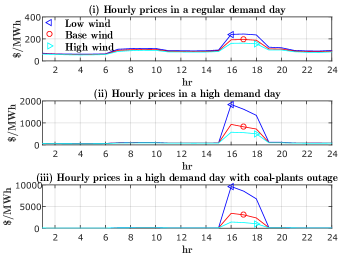
Figure 1: Hourly wholesale electricity prices in SA with $\phi=50\%$ and no storage.

Fig. 2 shows the minimum required (strategic/regulated) storage capacities for achieving various levels of price volatility in SA during a high demand day with coal plants outage. The minimum storage capacities are calculated by solving the optimization problem (12) for the high demand day with coal-plants outage case with $\phi=50\%$. According to Fig. 2, a strategic storage firm requires a substantially larger capacity, compared with a regulated storage firm, to achieve a target price volatility level due to the selfish behavior of the storage firms. In fact, the strategic storage firms may sometimes withhold their available capacities and do not participate in the price volatility reduction as they do not always benefit from reducing the price. The price volatility in SA can be reduced by 80% using either 420 MWh strategic storage or 340 MWh regulated storage. Note that AEMO has forecasted about 500 $\rm MWh$ battery storage to be installed in SA until 2035 [33].

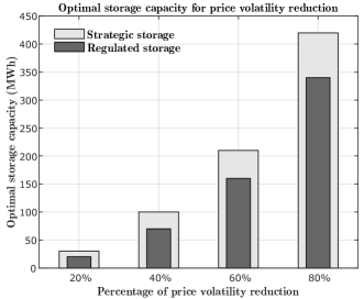
Figure 2: Optimal strategic and regulated storage capacity for achieving different price volatility levels in SA node with $\phi=50\%$ for a high demand day with coal-plants outage.

According to our numerical results, storage can displace the peaking generators, with high fuel costs and market power, which results in reducing the price level and the price volatility. A storage capacity of 500 MWh (or $\frac{500}{2}$ MW given the discharge coefficient $\eta^{\rm dis}=\frac{1}{2}$) reduces the square root of the price volatility from 2787 $/MWh to 919 $/MWh, almost 30% reduction, during a high demand day with coal-plant outage in SA.

The behaviour of the peak and the daily average prices for the high demand day with coal plants outage in SA is illustrated in Fig. 3. In this figure, the peak price represents the maximum of price over all scenarios during the day, i.e. $\max_{t,w}P_{tw}(\boldsymbol{q}^{\star}_{tw})$ and the daily average price indicates the average of price over time and scenarios, i.e. $\frac{1}{N_{T}}\sum_{tw}P_{tw}(q^{\star}_{tw})\Psi_{w}$. Sensitivity analysis of the peak and the daily average prices in SA with respect to storage capacity indicates that high storage capacities lead to relatively low prices in the market. At very high prices, demand is almost inelastic and a small amount of excess supply leads to a large amount of price reduction. According to Fig. 3, the rate of price reduction decreases as the storage capacity increases since large storage capacities lead to relatively low peak prices which make the demand more elastic.

Based on Fig. 3, the impact of storage on the daily average and peak prices depends on whether the storage firm is strategic or regulated. It can be observed that the impacts of strategic and regulated storage firms on the daily peak/average prices are almost similar for small storage capacities, i.e. when the storage capacity is smaller than 100 MWh (or $\frac{100}{2}$ MW given $\eta^{\rm dis}=\frac{1}{2}$). However, a regulated firm reduces both the peak and the average prices more efficiently compared with a strategic storage firm as its capacity becomes large. A large strategic storage firm in SA does not use its excess capacity beyond 500 MWh to reduce the market price since it acts as a strategic profit maximizer, but a regulated storage firm contributes to the price volatility reduction as long as there is potential for price reduction by its operation.

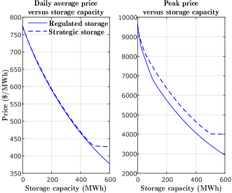
Figure 3: Daily peak and average prices in SA versus storage capacity with wind power fluctuation parameter $\phi=50\%$ in a high demand day with coal-plant outage.

Fig. 4 depicts the square root of price volatility in SA during the high demand day with coal plant outage for $\phi=50\%$ and $\phi=40\%$. According to this figure, the price volatility in the market decreases by installing either regulated or strategic storage devices. However, a strategic storage firm stops reducing the price volatility when its capacity exceeds a threshold value. Moreover, the square root of price volatility, in all cases, diminishes almost by 30% as the wind power fluctuation parameter decreases from 50% to 40%. Note that, as $\phi$ becomes small, the wind generation level becomes less volatile which results in a relatively low price volatility. This observation indicates that the required storage capacity to ensure a price volatility reduction target decreases as the wind power fluctuation parameter becomes small. Note that wind power fluctuation parameter $\phi$ can be reduced by improving the geographic diversity of wind farms in a region.

Based on Fig. 4, both price volatility and the required storage capacity for achieving a target price volatility become large as the wind power fluctuation parameter $\phi$ increases. To reduce the square root of price volatility to 1200 $/MWh, the required strategic capacity with $\phi=40\%$ and $\phi=50\%$ is 60 MWh and 70 MWh, respectively, more than that of a regulated storage. This observation confirms that regulated storage firms are more efficient than strategic firms in reducing the price volatility. Although storage alleviates the price volatility in the market, it is not capable to eliminate it completely.

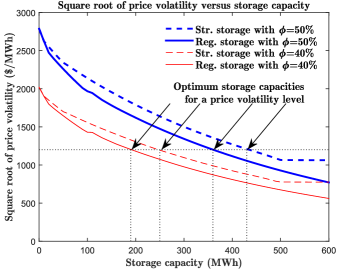
Figure 4: Square root of price volatility in SA versus storage capacity with $\phi$ equal to $40\%$ and $50\%$ during a high demand day with coal-plants outage.

V-B Two-node model simulations in South Australia and Victoria

In the previous subsection, we analysed the impact of storage on the price volatility in SA when the SA-VIC interconnector is not active. In this subsection, we first study the effect of the interconnector between SA and VIC on the price volatility in the absence of storage firms. Next, we investigate the impact of storage firms on the price volatility when the SA-VIC transmission line operates at various capacities. In our numerical results, SA is connected to VIC using a 680 MW interconnector which is currently operating with 70% of its capacity, i.e. 30% of its capacity is under maintenance. The numerical results in this subsection are based on the two-node model for a high demand day with coal plant outage in SA. To investigate the impact of transmission line on price volatility, it is assumed that the SA-VIC interconnector operates with 60% and 70% of its capacity.

According to our numerical results, the peak price in SA and VIC is equal to 9634 $/MWh when the SA-VIC interconnector is completely in outage and the wind power fluctuation parameter $\phi$ is equal to $50\%$. However, the peak price reduced to 1406 $/MWh and 1114 $/MWh when the interconnector operates at 60% and 70% of its capacity. The square root of price volatility is 2787 $/MWh, 303 $/MWh, and 219 $/MWh when the capacity of the SA-VIC transmission line is equal to 0%, 60%, and 70%, respectively.

Simulation results show that as long as the transmission line is not congested, the interconnector alleviates the price volatility phenomenon in SA by importing electricity from VIC to SA at peak times. Since the market in SA compared to VIC is much smaller, about three times, the price volatility abatement in SA after importing electricity from VIC is much higher than the price volatility increment in VIC. Moreover, the price volatility reduces as the capacity of transmission line increases.

Fig. 5 shows the optimum storage capacity versus the percentage of price volatility reduction in the two-node market. According to our numerical results, storage is just located in SA, which witnesses a high level of price volatility as the capacity of transmission line decreases. According to this figure, the optimum storage capacity becomes large as the capacity of transmission line decreases. Note that a sudden decrease of the transmission line capacity may result in a high level of price volatility in SA. However, based on Fig. 5, storage firms are capable of reducing the price volatility during the outage of the interconnecting lines.

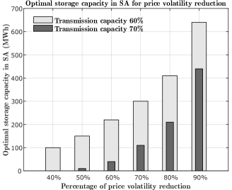
Figure 5: Optimal regulated storage capacity versus the percentage of price volatility reduction in the two-node market with wind power fluctuation parameter $\phi=50\%$ in a high demand day with coal-plants outage in SA.

VI Conclusion

High penetration of intermittent renewables, such as wind or solar farms, brings high levels of price volatility in electricity markets. Our study presents an optimization model which decides on the minimum storage capacity required for achieving a price volatility target in electricity markets. Based on our numerical results, the impact of storage on the price volatility in one-node electricity market of SA and two-node market of SA-VIC can be summarized as:

• Storage alleviates price volatility in the market due to the wind intermittency. However, storage does not remove price volatility completely, i.e. storage stops reducing the price volatility when it is not profitable.

• The effect of a storage firm on price volatility reduction depends on whether the firm is regulated or strategic. Both storage types have similar operation behaviour and price reduction effects when they possess small capacities. For larger capacities, a strategic firm may under-utilize its available capacity and stop reducing the price level due to its profit maximization strategy. On the other hand, a regulated storage firm is more efficient in price volatility reduction because of its social welfare maximization strategy. The price level and volatility reduction patterns observed when storage firms are regulated provide stronger incentives for the market operator to subsidize the storage technologies.

• Both storage devices and transmission lines are capable of reducing the price volatility. High levels of price volatility that may happen due to the line maintenance can be alleviated by storage devices.

We intend to study the impact of ancillary services markets [34] and capacity markets [35] on the integration of storage systems in electricity networks in our future work. We also plan to investigate the impacts of other factors in both demand and supply sides on the price volatility.

Appendix A Charging/Discharging

In this appendix, we show that the charge and discharge levels of any storage device cannot be simultaneously positive at the NE of the lower game. Consider a strategy in which both charge and discharge levels of storage device $i$ at time $t$ under scenario $w$, i.e. $q^{\rm dis}_{itw},q^{\rm ch}_{itw}$, are both positive. We show that this strategy cannot be a NE strategy as follows. The net electricity flow of storage can be written as $q^{\rm s}_{itw}=\eta^{\rm dis}_{i}q^{\rm dis}_{itw}-\frac{q^{\rm ch}_{itw}}{\eta^{\rm ch}_{i}}$. Let $\bar{q}^{\rm dis}_{itw}$ and $\bar{q}^{\rm ch}_{itw}$ be the new discharge and charge levels of storage firm $i$ defined as $\Big{\{}{{\bar{q}}^{\rm dis}_{itw}}=q^{\rm dis}_{itw}-\frac{q^{\rm ch}_{itw}}{\eta^{\rm dis}_{i}\eta^{\rm ch}_{i}},\quad{{\bar{q}}^{\rm ch}_{itw}}=0\Big{\}}$ if $q^{\rm s}_{itw}>0$, or $\Big{\{}{{\bar{q}}^{\rm dis}_{itw}}=0,\quad{{\bar{q}}^{\rm ch}_{itw}}=q^{\rm ch}_{itw}-q^{\rm dis}_{itw}\eta^{\rm dis}_{i}\eta^{\rm ch}_{i}\Big{\}}$ if $q^{\rm s}_{itw}<0$. The new net flow of electricity can be written as $\bar{q}^{\rm s}_{itw}=\eta^{\rm dis}_{i}{{\bar{q}}^{\rm dis}_{itw}}-\frac{{{\bar{q}}^{\rm ch}_{itw}}}{\eta^{\rm ch}_{i}}$. Note that the new variables $\bar{q}^{\rm s}_{itw}$, ${{\bar{q}}^{\rm ch}_{itw}}$ and ${{\bar{q}}^{\rm dis}_{itw}}$ satisfy the constraints (5b-5e).

Considering the new charge and discharge strategies ${{\bar{q}}^{\rm dis}_{itw}}$ and ${{\bar{q}}^{\rm ch}_{itw}}$, instead of $q^{\rm dis}_{itw}$ and $q^{\rm ch}_{itw}$, the nodal price and the net flow of storage device $i$ do not change. However, the charge/discharge cost of the storage firm $i$, under the new strategy, is reduces by:

$$c_{i}^{\rm s}\left(q^{\rm ch}_{itw}+q^{\rm dis}_{itw}\right)-c_{i}^{\rm s}\left({\bar{q}}^{\rm dis}_{itw}+{\bar{q}}^{\rm ch}_{itw}\right)>0$$

Hence, any strategy in which the charge and discharge variables are simultaneously positive cannot be a NE, i.e. at the NE of the lower game each storage firm is either in the charge mode or discharge mode.

References

- [1] J. C. Ketterer, “The impact of wind power generation on the electricity price in Germany,” Energy Economics, vol. 44, pp. 270–280, 2014.
- [2] D. Wozabal, C. Graf, and D. Hirschmann, “The effect of intermittent renewables on the electricity price variance,” OR spectrum, pp. 1–23, 2014.
- [3] C.-K. Woo, I. Horowitz, J. Moore, and A. Pacheco, “The impact of wind generation on the electricity spot-market price level and variance: The Texas experience,” Energy Policy, vol. 39, no. 7, pp. 3939–3944, 2011.
- [4] S.-J. Deng and S. S. Oren, “Electricity derivatives and risk management,” Energy, vol. 31, no. 6, pp. 940–953, 2006.
- [5] H. Higgs and A. Worthington, “Stochastic price modeling of high volatility, mean-reverting, spike-prone commodities: The Australian wholesale spot electricity market,” Energy Economics, vol. 30, p. 3172–3185, 2008.
- [6] D. Chattopadhyay and T. Alpcan, “A game-theoretic analysis of wind generation variability on electricity markets,” Power Systems, IEEE Transactions on, vol. 29, no. 5, pp. 2069–2077, Sept 2014.
- [7] AEMC, “Potential generator market power in the NEM,” Australian Energy Market Commission, Tech. Rep., 26 April 2013.
- [8] N. Li, C. Uçkun, E. M. Constantinescu, J. R. Birge, K. W. Hedman, and A. Botterud, “Flexible operation of batteries in power system scheduling with renewable energy,” IEEE Transactions on Sustainable Energy, vol. 7, no. 2, pp. 685–696, April 2016.
- [9] V. Krishnan and T. Das, “Optimal allocation of energy storage in a co-optimized electricity market: Benefits assessment and deriving indicators for economic storage ventures,” Energy, vol. 81, pp. 175 – 188, 2015.
- [10] A. Berrada and K. Loudiyi, “Operation, sizing, and economic evaluation of storage for solar and wind power plants,” Renewable and Sustainable Energy Reviews, vol. 59, pp. 1117 – 1129, 2016.
- [11] W. Qi, Y. Liang, and Z.-J. M. Shen, “Joint planning of energy storage and transmission for wind energy generation,” Operations Research, vol. 63, no. 6, pp. 1280–1293, 2015.
- [12] M. Sedghi, A. Ahmadian, and M. Aliakbar-Golkar, “Optimal storage planning in active distribution network considering uncertainty of wind power distributed generation,” IEEE Transactions on Power Systems, vol. 31, no. 1, pp. 304–316, Jan 2016.
- [13] L. Zheng, W. Hu, Q. Lu, and Y. Min, “Optimal energy storage system allocation and operation for improving wind power penetration,” IET Generation, Transmission Distribution, vol. 9, no. 16, pp. 2672–2678, 2015.
- [14] J. Xiao, Z. Zhang, L. Bai, and H. Liang, “Determination of the optimal installation site and capacity of battery energy storage system in distribution network integrated with distributed generation,” IET Generation, Transmission Distribution, vol. 10, no. 3, pp. 601–607, 2016.
- [15] Y. Zheng, Z. Y. Dong, F. J. Luo, K. Meng, J. Qiu, and K. P. Wong, “Optimal allocation of energy storage system for risk mitigation of discos with high renewable penetrations,” IEEE Transactions on Power Systems, vol. 29, no. 1, pp. 212–220, Jan 2014.
- [16] R. Walawalkar, J. Apt, and R. Mancini, “Economics of electric energy storage for energy arbitrage and regulation in new york,” Energy Policy, vol. 35, no. 4, pp. 2558 – 2568, 2007.
- [17] H. Mohsenian-Rad, “Optimal bidding, scheduling, and deployment of battery systems in california day-ahead energy market,” IEEE Transactions on Power Systems, vol. 31, no. 1, pp. 442–453, Jan 2016.
- [18] H. Akhavan-Hejazi and H. Mohsenian-Rad, “A stochastic programming framework for optimal storage bidding in energy and reserve markets,” in Innovative Smart Grid Technologies (ISGT), 2013 IEEE PES, Feb 2013, pp. 1–6.
- [19] H. Mohsenian-Rad, “Coordinated price-maker operation of large energy storage units in nodal energy markets,” IEEE Transactions on Power Systems, vol. 31, no. 1, pp. 786–797, Jan 2016.
- [20] E. Nasrolahpour, S. J. Kazempour, H. Zareipour, and W. D. Rosehart, “Strategic sizing of energy storage facilities in electricity markets,” IEEE Transactions on Sustainable Energy, vol. 7, no. 4, pp. 1462–1472, Oct 2016.
- [21] M. Ventosa, R. Denis, and C. Redondo, “Expansion planning in electricity markets. Two different approaches,” in Proceedings of the 14th Power Systems Computation Conference (PSCC), Seville, 2002.
- [22] W.-P. Schill, C. Kemfert et al., “Modeling strategic electricity storage: the case of pumped hydro storage in Germany,” Energy Journal-Cleveland, vol. 32, no. 3, p. 59, 2011.
- [23] J. B. Cardell, C. C. Hitt, and W. W. Hogan, “Market power and strategic interaction in electricity networks,” Resource and Energy Economics, vol. 19, no. 1–2, pp. 109 – 137, 1997.
- [24] W. W. Hogan, “A market power model with strategic interaction in electricity networks,” The Energy Journal, vol. 18, no. 4, pp. 107–141, 1997.
- [25] E. G. Kardakos, C. K. Simoglou, and A. G. Bakirtzis, “Optimal bidding strategy in transmission-constrained electricity markets,” Electric Power Systems Research, vol. 109, pp. 141 – 149, 2014.
- [26] AEMO, “An Introduction to Australia’s National Electricity Market,” Australian Energy Market Operator, Tech. Rep., 2010.
- [27] D. Fudenberg and J. Tirole, Game theory. Cambridge, Mass. : M.I.T. Press, 1991.
- [28] M. C. Ferris and T. S. Munson, “GAMS/PATH user guide: Version 4.3,” Washington, DC: GAMS Development Corporation, 2000.
- [29] J. M. Morales, S. Pineda, A. J. Conejo, and M. Carrion, “Scenario reduction for futures market trading in electricity markets,” IEEE Transactions on Power Systems, vol. 24, no. 2, pp. 878–888, 2009.
- [30] AEMO, “South Australian Wind Study Report,” Australian Energy Market Operator, Tech. Rep., 2013.
- [31] H. Ding, Z. Hu, and Y. Song, “Stochastic optimization of the daily operation of wind farm and pumped-hydro-storage plant,” Renewable Energy, vol. 48, pp. 571–578, 2012.
- [32] AER, “State of the energy market 2015,” Australian Energy Regulator, Tech. Rep., 2015.
- [33] AEMO, “Roof-top PV Information Paper, National Electricity Forecasting,” Australian Energy Market Operator, Tech. Rep., 2012.
- [34] D. Chattopadhyay, “Multicommodity spatial cournot model for generator bidding analysis,” Power Systems, IEEE Transactions on, vol. 19, no. 1, pp. 267–275, Feb 2004.
- [35] D. Chattopadhyay and T. Alpcan, “Capacity and energy-only markets under high renewable penetration,” Power Systems, IEEE Transactions on, vol. PP, no. 99, pp. 1–11, 2015.