Categorification of invariants in gauge theory and sypmplectic geometry

Abstract.

This is a mixture of survey article and research anouncement. We discuss Instanton Floer homology for 3 manifolds with boundary. We also discuss a categorification of the Lagrangian Floer theory using the unobstructed immersed Lagrangian correspondence as a morphism in the category of symplectic manifolds.

During the year 1998-2012, those problems have been studied emphasising the ideas from analysis such as degeneration and adiabatic limit (Instanton Floer homology) and strip shrinking (Lagrangian correspondence). Recently we found that replacing those analytic approach by a combination of cobordism type argument and homological algebra, we can resolve various difficulties in the analytic approach. It thus solves various problems and also simplify many of the proofs.

1. Introduction and review

The research defining invariants by using moduli spaces in differential geometry and topology started around 1980’s. One of its first example is Donaldson’s polynomial invariant of smooth 4 manifolds [D3]. Various ‘quantum’ invariants of knots which appeared around the same time have similar flavor and actually they turn out to be closely related to each other. (Instanton) Floer homology of 3 manifolds (homology 3 spheres) appeared late 1980’s [Fl2] and it was soon realized that Instanton Floer homology provides the basic frame work to define a relative version of Donaldson invariant. The notion of topological field theory was introduced by Witten [Wi1] inspired by this relative Donaldson invariant. Soon after that Witten [Wi2] found an invariant of 3 manifolds (possibly equipped with knot and link) and its relative version. This is a generalization of quantum invariant of knot. The relative version of Witten’s invariant uses conformal block as its 2 dimensional counterpart. Segal [Se1, Se2] introduced categorical formulation of conformal field theory and of several related theories. Since then various categorifications have been introduced and studied by many mathematicians. In this article the author surveys some of them where $A_{\infty}$ category appears.

The gauge theory invariant we discuss in this article is one in the column $n=4$, of the next table.

	invariants	Case $n=4$	Case $n=3$
$n$	number	Donaldson invariant	Witten’s invariant
$n-1$	group	Floer homology	Conformal block
$n-2$	category	$\mathfrak{Fuk}(R(\Sigma))$	representation of loop group

Table 1

We begin with a quick review of 4 and 3 dimensional invariants.

1.1. Donaldson invariant

Let $X$ be an oriented 4 manifold and $\mathcal{P}_{X}\to X$ either a principal $SO(3)$ or $SU(2)$ bundle. (We denote $G=SO(3)$ or $SU(2)$.) We take a Riemannian metric on $X$, which induces Hodege $*$ operator on differential $k$ forms.

$$*:\Omega^{k}(X)\to\Omega^{4-k}(X).$$

On $2$ forms we have $**=1$. Therefore $\Omega^{2}(X)$ is decomposed into a direct sum

$$\Omega^{2}(X)=\Omega_{+}^{2}(X)\oplus\Omega^{2}_{-}(X),\qquad\Omega_{\pm}^{2}(X)=\{u\in\Omega^{2}(X)\mid*u=\pm u\}.$$

Let $ad(\mathcal{P}_{X})=\mathcal{P}_{X}\times_{G}\mathfrak{g}$ be the Lie algebra ($\mathfrak{g}=so(3)$ or $su(2)$) bundle associated to $\mathcal{P}_{X}$ by the adjoint representation $G\to{\rm Aut}(\mathfrak{g})$. For a connection $A$ of $\mathcal{P}_{X}$ its curvature $F_{A}$ is a section of $\Omega^{2}(X)\otimes ad(\mathcal{P}_{X})$. We decompose it to

$$F_{A}=F_{A}^{+}+F_{A}^{-}$$

where $F_{A}^{\pm}$ is a section of $\Omega^{2}_{\pm}(X)\otimes ad(\mathcal{P}_{X})$.

A connection $A$ is called an Anti-Self-Dual (or ASD) connection if $F_{A}^{+}=0$.

We denote by $\mathcal{A}(\mathcal{P}_{X})$ the set of all (smooth) connections on $\mathcal{P}_{X}$ and $\mathcal{G}(\mathcal{P}_{X})$ the set of all (smooth) gauge transformations of $\mathcal{P}_{X}$. (The later is the set of all smooth sections of the bundle $Ad(\mathcal{P}_{X})=\mathcal{P}_{X}\times_{G}G$ which is associated to $\mathcal{P}_{X}$ by the adjoint action of $G$ on $G$.) The group $\mathcal{G}(\mathcal{P}_{X})$ acts on $\mathcal{A}(\mathcal{P}_{X})$ and we denote by $\mathcal{B}(\mathcal{P}_{X})$ the quotient space.

We denote by $\mathcal{M}(\mathcal{P}_{X})\subset\mathcal{B}(\mathcal{P}_{X})$ the set of all $\mathcal{G}(\mathcal{P}_{X})$ equivalence classes of ASD connections.

In the simplest case, the Donaldson invariant of $X$ is the order of the set $\mathcal{M}(\mathcal{P}_{X})$ (counted with appropriate sign), and is an integer. More generally it is regarded as a polynomial map $H^{*}(\mathcal{B}(\mathcal{P}_{X}))\to{\mathbb{Z}}$ obtained by

$$c\mapsto\int_{\mathcal{M}(\mathcal{P}_{X})}c.$$ (1.1)

Actually since $\mathcal{M}(\mathcal{P}_{X})$ is non-compact, we need to study the behavior of the cohomology class $c$ at infinity of $\mathcal{M}(\mathcal{P}_{X})$, carefully. Another problem is that $\mathcal{M}(\mathcal{P}_{X})$ has in general a singularity. We do not discuss these points in this section. Donaldson used a map $\mu:H_{2}(X)\to H^{2}(\mathcal{B}(\mathcal{P}_{X})).$ This map is defined by the slant product $c\mapsto p_{1}/c$, where $p_{1}$ is 1st Pontriagin or second Chern class of the universal bundle on $\mathcal{B}(\mathcal{P}_{X})\times X$.

On the subring generated by the image of this map $\mu$, the integration (1.1) behaves nicely and defines an invariant. (We need to assume that the number $b_{2}^{+}$ which is the sum of the multiplicities of positive eigenvalues of the intersection form on $H_{2}(X;{\mathbb{Q}})$, is not smaller than $2$, for this invariant to be well defined.) In that case, we have a multi-linear map on $H_{2}(X)$ which is called Donaldson’s polynomial invariant. We denote it by

$$Z(c_{1},\dots,c_{k};\mathcal{P}_{X})=\int_{\mathcal{P}_{X}}\mu(c_{1})\wedge\dots\wedge\mu(c_{k})\in{\mathbb{Z}}$$ (1.2)

for $c_{i}\in H_{2}(X)$. Note the integration makes sense only when

$$\dim\mathcal{M}(\mathcal{P}_{X})=2k,$$

($\deg c_{i}=2$). The dimension of $\mathcal{M}(\mathcal{P}_{X})$ is determined by the seond Chern (or the first Pontriagin) number of $\mathcal{P}_{X}$. So if we fix the second Stiefel-Whiteney class of $\mathcal{P}_{X}$ the isomorphism class of bundle $\mathcal{P}_{X}$ for which (1.2) can be nonzero is determined by $k$. So we omit $\mathcal{P}_{X}$ and write $Z(c_{1},\dots,c_{k})$ sometimes.

1.2. Floer homology (Instanton homology)

Let $M$ be a 3 manifold and $\mathcal{P}_{M}$ a principal $G=SO(3)$ or $SU(2)$ bundle on it.

Assumption 1.1.

We assume that one of the following two conditions is satisfied.

1. $G=SO(3)$ and $w^{2}(\mathcal{P}_{M})\neq 0\in H^{2}(M;{\mathbb{Z}}_{2})$. (Here $w^{2}(\mathcal{E}_{P})$ is the second Stiefel-Whiteney class.)

2. $G=SU(2)$ and $H(M;{\mathbb{Z}})\cong H(S^{3};{\mathbb{Z}})$.

The notation $\mathcal{A}(\mathcal{P}_{M})$, $\mathcal{G}(\mathcal{P}_{M})$, $\mathcal{B}(\mathcal{P}_{M})$ are defined in the same way as the 4 dimensional case. We denote by $R(M;\mathcal{P}_{M})\subset\mathcal{B}(\mathcal{P}_{M})$ the set of all flat connections.

We assume the following for the simplicity of description.

Assumption 1.2.

1. The set $R(M;\mathcal{P}_{M})$ is a finite set.

2. For any $[a]\in R(M;\mathcal{P}_{M})$ the cohomology group $H^{1}(M;ad_{a}(\mathcal{P}_{M}))$ vanishes. Here the first cohomology group $H^{1}(M;ad_{a}(\mathcal{P}_{M}))$ is defined by the complex

   $$ad\,\mathcal{P}_{M}\otimes\Omega^{0}\overset{d_{a}}{\longrightarrow}ad\,\mathcal{P}_{M}\otimes\Omega^{1}\overset{d_{a}}{\longrightarrow}ad\,\mathcal{P}_{M}\otimes\Omega^{2}.$$

   (Note $d_{a}\circ d_{a}=0$ since $F_{a}=0$.)

Remark 1.3.

We can remove this assumption by appropriately perturbing the defining equation $F_{a}=0$ of $R(M;\mathcal{P}_{M})$ in a way similar to [D1, Fl2, He].

In case Assumption 1.1 (2) is satisfied we put $R_{0}(M;\mathcal{P}_{M})=R(M;\mathcal{P}_{M})\setminus\{[0]\}$, where $[0]$ is the gauge equivalence class of the trivial connection. In case of Assumption 1.1 (1), we put $R_{0}(M;\mathcal{P}_{M})=R(M;\mathcal{P}_{M})$.

We define ${\mathbb{Z}}_{2}$ vector space $CF(M;\mathcal{P}_{M})$ whose basis is identified with $R(M;\mathcal{P}_{M})$. We define a boundary operator

$$\partial:CF(M;\mathcal{P}_{M})\to CF(M;\mathcal{P}_{M})$$

as follows. Let $[a],[b]\in R_{0}(M;\mathcal{P}_{M})$. We fix their representatives $a,b$. We consider the set of connections $A$ of the bundle $\mathcal{P}_{M}\times{\mathbb{R}}$ on $M\times{\mathbb{R}}$ with the following properties. We use $\tau$ as the coordinate of ${\mathbb{R}}$.

1. $F_{A}^{+}=0$.

2. The $L^{2}$ norm of the curvature

   $$\int_{M\times{\mathbb{R}}}\|F_{A}\|^{2}{\rm vol}_{M}d\tau$$

   is finite.

3. We require

   $$\lim_{\tau\to-\infty}A=a,\qquad\lim_{\tau\to+\infty}A=b.$$

Remark 1.4.

We can use Assumption 1.2 (2) to show that if (IF.3) is satisfied then the convergence is automatically of exponential order.

We denote by $\widetilde{\mathcal{M}}(M\times{\mathbb{R}};a,b)$ the set of all gauge equivalence classes of the connections $A$ satisfying the above conditions (IF.1), (IF.2), (IF.3).

The ${\mathbb{R}}$ action induced by the translation of ${\mathbb{R}}$ factor in $M\times{\mathbb{R}}$ induces an ${\mathbb{R}}$ action on $\widetilde{\mathcal{M}}(M\times{\mathbb{R}};a,b)$. We denote the quotient space by this action by ${\mathcal{M}}(M\times{\mathbb{R}};a,b)$.

Theorem 1.5.

(Floer) We can define a map $\mu:R_{0}(M;\mathcal{P}_{M})\to{\mathbb{Z}}_{4}$ ($SO(3)$ case) or ${\mathbb{Z}}_{8}$ ($SU(2)$ case) such that:

1. ${\mathcal{M}}(M\times{\mathbb{R}};a,b)$ is decomposed into pieces ${\mathcal{M}}(M\times{\mathbb{R}};a,b;k)$ where $k+1$ is a natural number congruent to $\mu(b)-\mu(a)$.

2. By ‘generic’ perturbation we may assume that ${\mathcal{M}}(M\times{\mathbb{R}};a,b;k)$ is compactified to a manifold with corners of dimention $k$, outside the singularity set of codimension $\geq 2$.

3. Moreover the boundary of ${\mathcal{M}}(M\times{\mathbb{R}};a,b;k)$ is identified with the disjoint union of the direct product

   $${\mathcal{M}}(M\times{\mathbb{R}};a,c;k_{1})\times{\mathcal{M}}(M\times{\mathbb{R}};c,b;k_{2})$$ (1.3)

   where $c\in R_{0}(M;\mathcal{P}_{M})$ and $k_{1}+k_{2}+1=k$.

Now we define

$$\langle\partial[a],[b]\rangle\equiv\#{\mathcal{M}}(M\times{\mathbb{R}};a,c;0)\mod 2,$$

and

$$\partial[a]=\sum_{[b];\mu(b)=\mu(a)-1}\langle\partial([a]),[b]\rangle[b].$$ (1.4)

Theorem 1.5 (3) implies that the union of the spaces (1.3) over $c$ and $k_{1},k_{2}$ with $k_{1}+k_{2}$ given is a boundary of some spaces. Especially in case $k_{1}=k_{2}=0$ the union of (1.3) over $c$ is a boundary of $1$ dimensional manifold and so its order is even. It implies:

$$\sum_{c}\#\langle\partial[a],[c]\rangle\langle\partial[c],[b]\rangle=0.$$

Namely $\partial\partial[a]=0$.

Definition 1.6.

$$HF(M;\mathcal{P}_{M})\cong\frac{{\rm Ker}\,\,\,\left(\partial:CF(M;\mathcal{P}_{M})\to CF(M;\mathcal{P}_{M}\right)}{{\rm{Im}}\,\,\,\left(\partial:CF(M;\mathcal{P}_{M})\to CF(M;\mathcal{P}_{M})\right)}.$$

We call this group (${\mathbb{Z}}_{2}$ vector space) the Instanton Floer homology of $(M,\mathcal{P}_{M})$. Actually we can put orientation of the moduli space we use and then define Floer homology group over ${\mathbb{Z}}$.

Floer ([Fl2, Fl3]) proved that the group $HF(M;\mathcal{P}_{M})$ is independent of various choices made in the definitions.

The idea behind this definition is to study the following Chern-Simons functional. We consider the case when $\mathcal{P}_{M}$ is an $SU(2)$ bundle which is necessary trivial as a smooth $SU(2)$ bundle. We fix a trivialization and then an element of $\mathcal{A}(\mathcal{P}_{M})$ is identified with an $su(2)$ valued one form $a$. We may regard it as a $2\times 2$ matrix valued one form. We then put

$$\mathfrak{cs}(a)=\frac{1}{4\pi^{2}}\int_{M}Tr\left(\frac{1}{2}a\wedge da+\frac{1}{3}a\wedge a\wedge a\right).$$ (1.5)

This functional descents to a map $\mathcal{B}(\mathcal{P}_{M})\to{\mathbb{R}}/{\mathbb{Z}}$. In fact if we regard a gauge transformation as a map $M\to SU(2)$ we have

$$\mathfrak{cs}(g^{*}a)=\mathfrak{cs}(a)+\deg g.$$

On the other hand any connection $A$ of $\mathcal{P}_{M}\times{\mathbb{R}}$ on $M\times{\mathbb{R}}$ can be transformed to a connection without $d\tau$ component by a gauge transformation. (Note $\tau$ is the coordinate of ${\mathbb{R}}$.) We call it the temporal gauge. If we take the temporal gauge and $A|_{M\times\{\tau\}}=a(\tau)$ then the equation $F_{A}^{+}=0$ is equivalent to

$$\frac{d}{d\tau}a(\tau)={\rm grad}_{a(\tau)}\mathfrak{cs}.$$ (1.6)

Here the right hand side is defined by

$$\langle{\rm grad}_{a}\mathfrak{cs},a^{\prime}\rangle=\left.\frac{d}{ds}\mathfrak{cs}(a+sa^{\prime})\right|_{s=0}.$$

($\langle\cdot,\cdot\rangle$ is the $L^{2}$ inner product.) So $HF(M;\mathcal{P}_{M})$ is regarded as a Morse homology of $\mathfrak{cs}$. There is a similar functional in the $SO(3)$ case.

1.3. Relative Donaldson invariant

The relation between Donaldson invariant and Floer homology is described as follows.

Let $X_{1}$ and $X_{2}$ be oriented 4 manifolds with boundary $M$ and $-M$, respectively. We glue $X_{1}$ and $X_{2}$ at $M$ to obtain a closed oriented 4 manifold $X$. We consider the case $H_{1}(M;{\mathbb{Q}})=0$. Then

$$H_{2}(X;{\mathbb{Q}})=H_{2}(X_{1};{\mathbb{Q}})\oplus H_{2}(X_{2};{\mathbb{Q}}).$$ (1.7)

We also assume $b_{2}^{+}(X_{i})$, the sum of multiplicities of positive eigenvalues of the intersection form on $H_{2}(X_{i};{\mathbb{Q}})$, is at least $2$.

We remark that

$$R_{0}(M;\mathcal{P}_{M})\cong R_{0}(-M;\mathcal{P}_{M}).$$

The map ${\mathbb{R}}\times M\to{\mathbb{R}}\times-M$ which sends $(\tau,x)$ to $(-\tau,x)$ is an orientation preserving diffeomorphism. So

$$\langle\partial_{M}a,b\rangle=\langle a,\partial_{-M}b\rangle$$

Therefore the boundary operator $\partial_{-M}$ is the dual to $\partial_{M}$. We thus obtain a pairing:

$$\langle\cdot,\cdot\rangle:HF(M;\mathcal{P}_{M})\times HF(-M;\mathcal{P}_{M})\to{\mathbb{Z}}.$$

Theorem 1.7.

(Floer-Donaldson, See [Fu3, D5])

1. If $\partial X_{1}=M$ and $\left.\mathcal{P}_{X_{1}}\right|_{M}=\mathcal{P}_{M}$, then there exists a multilinear map

   $$Z(\cdot;{X_{1}},\mathcal{P}_{X_{1}}):H_{2}(X_{1};{\mathbb{Z}})^{\otimes k}\to HF(M;\mathcal{P}_{M}).$$

2. In the situation we mentioned at the beginning of this subsection we have

   $$\langle Z(c_{1,1},\dots,c_{1,k_{1}};\mathcal{P}_{X_{1}}),Z(c_{2,1},\dots,c_{2,k_{2}};\mathcal{P}_{X_{2}})\rangle$$ (1.8)

   $$=Z(c_{1,1},\dots,c_{1,k_{1}},c_{2,1},\dots,c_{2,k_{2}};\mathcal{P}_{X}).$$

The construction of relative invariant in Theorem 1.7 roughly goes as follows. We take a Riemannian metric on $X_{1}\setminus\partial X_{1}$ such that it is isometric to the direct product $M\times[0,\infty)$ outside a compact set. Let $a$ be a flat connection with $[a]\in R_{0}(M;\mathcal{P}_{M})$.

We consider the set of connections $A$ of $\mathcal{P}_{X}$ such that

1. $F_{A}^{+}=0$.

2. The $L^{2}$ norm of the curvature $\int_{X_{1}}\|F_{A}\|^{2}{\rm vol}_{X_{1}}$ is finite.

3. We require $\lim_{\tau\to+\infty}A|_{M\times\{\tau\}}=a.$

We denote the set of gauge equivalence classes of such $A$ by $\mathcal{M}(X_{1};a;\mathcal{P}_{X_{1}})$ and define

$$Z(c_{1,1},\dots,c_{1,k_{1}};{X_{1}},\mathcal{P}_{X_{1}})$$

$$=\sum_{a\in R_{0}(M;\mathcal{P}_{M})}\left(\int_{\mathcal{M}(X_{1};a;\mathcal{P}_{X_{1}})}\mu(c_{1,1})\wedge\dots\wedge\mu(c_{1,k_{1}})\right)[a].$$

We can show that this is a cycle in $CF(M;\mathcal{P}_{M})$ by studying the boundary of the moduli space $\mathcal{M}(X_{1};a;\mathcal{P}_{X_{1}})$, that is,

$$\partial\mathcal{M}(X_{1};a;\mathcal{P}_{X_{1}})=\bigcup_{b}\mathcal{M}(X_{1};b;\mathcal{P}_{X_{1}})\times\mathcal{M}(M\times{\mathbb{R}};b,a).$$

To show (1.8) we consider the following sequence of metrics on $X$. We take compact subsets $K_{i}$ of $X_{i}$ such that

$${\rm Int}\,X_{1}\setminus K_{1}\cong M\times(0,\infty),\qquad{\rm Int}\,X_{2}\setminus K_{2}\cong M\times(-\infty,0).$$

We put

$$X(T)=(K_{1}\cup M\times(0,T/2])\cup(M\times[-T/2,0]\cup K_{2})$$

where we identify $M\times\{T/2\}\cong M\times\{-T/2\}$. $X(T)$ is diffeomorphic to $X$ and has an obvious Riemannian metric. So we obtain the moduli space $\mathcal{M}(X(T);\mathcal{P}_{X})$. We have

$$Z(c_{1,1},\dots,c_{1,k_{1}},c_{2,1},\dots,c_{2,k_{2}};\mathcal{P}_{X})=\int_{\mathcal{M}(X(T);\mathcal{P}_{X})}\mu(c_{1,1})\wedge\dots\wedge\mu(c_{2,k_{2}})$$

for any $T$.

Then (1.8) will be a consequence of the next equality.

$$\lim_{T\to\infty}\mathcal{M}(X(T);\mathcal{P}_{X})=\bigcup_{a\in R_{0}(M;\mathcal{P}_{M})}\mathcal{M}(X_{1};a;\mathcal{P}_{X_{1}})\times\mathcal{M}(X_{2};a;\mathcal{P}_{X_{2}}).$$ (1.9)

2. Invariant in dimension 4-3-2

The idea to extend the story of subsections 1.1, 1.2, 1.3 so that it includes dimension 2 was studied by various mathematicians in 1990’s. (See for example [Fu2, Fu5].) It can be summarized as follows.

Problem 2.1.

1. For each pair of an oriented 2 manifold $\Sigma$ and a principal $G$-bundle $\mathcal{P}_{\Sigma}$ on it, associate a category $\mathcal{C}(\Sigma;\mathcal{P}_{\Sigma})$, such that for each two objects of $\mathcal{C}(\Sigma;\mathcal{P}_{\Sigma})$ the set of morphisms between them is an abelian group.

2. For any pair $(M,\mathcal{P}_{M})$ of an oriented $3$ manifold $M$ with boundary and a principal $G$-bundle $\mathcal{P}_{M}$ on it, associate an object $HF_{(M,\mathcal{P}_{M})}$ of $\mathcal{C}(\Sigma;\mathcal{P}_{M}|_{\Sigma})$, where $\Sigma=\partial M$.

3. Let $(M_{1},\mathcal{P}_{M_{1}})$, $(M_{2},\mathcal{P}_{M_{2}})$ be pairs as in (2) such that $\partial M_{1}=-\partial M_{2}=\Sigma$, $\mathcal{P}_{\Sigma}=\mathcal{P}_{M_{1}}|_{\Sigma}=\mathcal{P}_{M_{2}}|_{\Sigma}$. We glue them to obtain $(M,\mathcal{P}_{M})$. Then show:

   $$HF(M;\mathcal{P}_{M})=\mathcal{C}(HF_{(M_{1},\mathcal{P}_{M_{1}})},HF_{(M_{2},\mathcal{P}_{M_{2}})}).$$ (2.1)

   Here the left hand side is the Instanton Floer homology as in Definition 1.6 and the right hand side is the set of morphisms in the category $\mathcal{C}(\Sigma;\mathcal{P}_{M}|_{\Sigma})$, which is an abelian group.

There is a formulation which include the case

$$\partial(M,\mathcal{P}_{M})=-(\Sigma_{1},\mathcal{P}_{\Sigma_{1}})\sqcup(\Sigma_{2},\mathcal{P}_{\Sigma_{2}}).$$

See Section 8. We may join it with 4+3 dimensional picture so that we include the case of 4 manifold with corner.

An idea to find such category $\mathcal{C}(\Sigma;\mathcal{P}_{\Sigma})$ is based on the fact that the space of all flat connections $R(\Sigma;\mathcal{P}_{\Sigma})$ has a symplectic structure, which we define below.

Let $[\alpha]\in R(\Sigma;\mathcal{P}_{\Sigma})$. The tangent space $T_{\alpha}R(\Sigma;\mathcal{P}_{\Sigma})$ is identified with the first cohomology

$$H^{1}(\Sigma,ad_{\alpha}(\mathcal{P}_{\Sigma}))=\frac{{\rm Ker}\left(d_{\alpha}:\mathcal{P}_{M}\otimes\Omega^{1}\overset{d_{\alpha}}{\longrightarrow}ad\,\mathcal{P}_{M}\otimes\Omega^{2}\right)}{{\rm Im}\left(d_{\alpha}:\mathcal{P}_{M}\overset{d_{\alpha}}{\longrightarrow}ad\,\mathcal{P}_{M}\otimes\Omega^{1}\right)}.$$

The symplectic form $\omega$ at $T_{\alpha}R(\Sigma;\mathcal{P}_{\Sigma})\cong H^{1}(\Sigma,ad_{\alpha}(\mathcal{P}_{\Sigma}))$ is given by

$$\omega([u],[v])=\int_{\Sigma}Tr(u\wedge v).$$

(See [Go].) We can prove that this 2 form $\omega$ is a closed two form based on the fact that $R(\Sigma;\mathcal{P}_{\Sigma})$ is regarded as a symplectic quotient

$$\mathcal{A}(\Sigma,\mathcal{P}_{\Sigma})/\!/\mathcal{G}(\Sigma,\mathcal{P}_{\Sigma}).$$

In fact we may regard the curvature

$$\alpha\mapsto F_{\alpha}\in C^{\infty}(\Sigma;ad_{\alpha}\mathcal{P}\otimes\Omega^{2})$$

as the moment map of the action of gauge transformation group $\mathcal{G}(\Sigma,\mathcal{P}_{\Sigma})$ on $\mathcal{A}(\Sigma,\mathcal{P}_{\Sigma})$. (See [AB].)

We next consider $(M,\mathcal{P}_{M})$ as in Problem 2.1 (2). By the same reason as Assumption 1.2 we assume:

Assumption 2.2.

1. The set $R(M;\mathcal{P}_{M})$ has a structure of a finite dimensional manifold.

2. For any $[a]\in R(M;\mathcal{P}_{M})$ the second cohomology $H^{2}(M;ad_{a}(\mathcal{P}_{M}))$ vanishes. Here the second cohomology group $H^{2}(M;ad_{a}(\mathcal{P}_{M}))$ is the cokernel of

   $$d_{a}:ad\,\mathcal{P}_{M}\otimes\Omega^{1}\longrightarrow ad\,\mathcal{P}_{M}\otimes\Omega^{2}.$$

Remark 2.3.

In Assumption 1.2 we assumed all the cohomology groups vanish. In fact in case $\partial M=\emptyset$ (and $M$ is 3 dimensional) we have

$$H^{2}(M;ad_{a}(\mathcal{P}_{M}))\cong(H^{1}(M;ad_{a}(\mathcal{P}_{M})))^{*}$$

by Poincaré duality. So vanishing of 2nd cohomology implies the vanishing of the 1st cohomology. The zero-th cohomology vanishes if the connection is irreducible. (Namely the set of all gauge transformations which preserve the connection $a$ is zero dimensional.)

We also remark that actually (2) implies (1).

We then have the next lemma.

Lemma 2.4.

We assume $\partial(M,\mathcal{P}_{M})=(\Sigma,\mathcal{P}_{\Sigma})$ and Assumption 2.2. Let $i:R(M;\mathcal{P}_{M})\to R(\Sigma;\mathcal{P}_{\Sigma})$ be the map induced by the restriction of the connection. Then

$$i^{*}\omega=0.$$

Here $\omega$ is the symplectic form of $R(\Sigma;\mathcal{P}_{\Sigma})$.

Proof.

This is an immediate consequence of Stokes’ theorem. ∎

Let $i(a)=\alpha$. We consider the exact sequence

$$0\rightarrow H^{1}(M;ad_{a}(\mathcal{P}_{M}))\rightarrow H^{1}(\Sigma;ad_{\alpha}(\mathcal{P}_{\Sigma}))\rightarrow H^{2}(M,\Sigma;ad_{a}(\mathcal{P}_{M}))\rightarrow 0$$ (2.2)

Note $H^{2}(M;ad_{a}(\mathcal{P}_{M}))\cong H^{1}(M,\Sigma;ad_{a}(\mathcal{P}_{M}))\cong 0$ by Assumption 2.2 (2) and Poincaré duality. Moreover $H^{1}(M;ad_{a}(\mathcal{P}_{M}))\cong H^{2}(M,\Sigma;ad_{a}(\mathcal{P}_{M}))^{*}$ by Poincaré duality. Thus (2.2) implies that

$$\dim R(M;\mathcal{P}_{M})=\frac{1}{2}\dim R(\Sigma;\mathcal{P}_{\Sigma})$$ (2.3)

if $\partial M=\Sigma$.

Corollary 2.5.

In the situation of Lemma 2.4, $R(M;\mathcal{P}_{M})$ is an immersed Lagrangian submanifold of $R(\Sigma;\mathcal{P}_{\Sigma})$ if $i:R(M;\mathcal{P}_{M})\to R(\Sigma;\mathcal{P}_{\Sigma})$ is an immersion.

We can again perturb the defining equation $F_{a}=0$ of $R(M;\mathcal{P}_{M})$ so that the assumption of Corollary 2.5 is satisfied in the modified form. Namely we obtain a Lagrangian immersion to $R(\Sigma;\mathcal{P}_{\Sigma})$ from a moduli space that is a perturbation of $R(M;\mathcal{P}_{M})$. This is proved by Herald [He]. He also proved that the Lagrangian cobordism class of the perturbed immersed Lagrangian submanifold is independent of the choice of the perturbation.

The above obserbations let the Donaldson make the next:

Proposal 2.6.

(Donaldson [D4]) The category $\mathcal{C}(\Sigma;\mathcal{P}_{\Sigma})$ is defined such that:

1. Its object is a Lagrangian submanifold of $R(\Sigma;\mathcal{P}_{\Sigma})$.

2. The set of morphisms from $L_{1}$ to $L_{2}$ is the Lagrangian Floer homology $HF(L_{1},L_{2})$.

3. The composition of the morphism is defined by counting the pseudo-holomorphic triangle as in Figure 1 below.

The first approximation of the object which we assign to $(M,\mathcal{P}_{M})$ is the immersed Lagrangian submanifold $R(\Sigma;\mathcal{P}_{\Sigma})$.

This proposal is made in 1992 at University of Warwick. There are various problems to realize this proposal which was known already at that stage to experts.

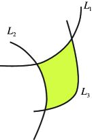
Figure 1. Holomorphic triangle

Difficulty 2.7.

1. The space $R(\Sigma;\mathcal{P}_{\Sigma})$ is in general singular. Symplectic Floer theory on a singular symplectic manifold is difficult to study.

2. Even in the case of smooth compact symplectic manifold, the Floer homology of two Lagrangian submanifolds is not defined in general and there are various conceptional and technical difficulties in doing so.

3. It is known that (Instanton) Floer homology of $M=M_{1}\cup_{\Sigma}M_{2}$ is not determined by the pair of Lagrangian submanifolds $R(M_{1};\mathcal{P}_{M_{1}})$ and $R(M_{2};\mathcal{P}_{M_{2}})$. So we need some additional information than the immersed Lagrangian submanifold $R(M;\mathcal{P}_{M})$ to obtain actual relative invariant. (This is the reason why Donaldson mentioned $R(M;\mathcal{P}_{M})$ as a first approximation and is not a relative invariant itself.)

I will explain how much in 25 years, after the proposal made in 1992, our understanding on these problems have been improved.

3. Relation to Atiyah-Floer conjecture

In this section we explain the relation of the discussion in the previous section to a famous conjecture called Atiyah-Floer conjecture [At]. In its original form Atiyah-Floer conjecture can be stated as follows. Let $M$ be a closed oriented 3 manifold such that $H_{1}(M;{\mathbb{Z}})=0$. We represent $M$ as

$$M=H^{1}_{g}\cup_{\Sigma_{g}}H^{2}_{g}.$$

where $H^{1}_{g}$ and $H^{2}_{g}$ are handle bodies with genus $g$ and $\Sigma_{g}=\partial H^{1}_{g}=\partial H^{2}_{g}$. We consider the trivial $SU(2)$ bundle $\mathcal{P}_{M}$ on $M$ and on $H^{i}_{g}$, $\Sigma_{g}$. Let $R(\Sigma_{g};\mathcal{P}_{\Sigma_{g}})$, $R(H^{i}_{g};\mathcal{P}_{H^{i}_{g}})$, $R(M;\mathcal{P}_{M})$ be the spaces of gauge equivalence classes of flat connections of the trivial $SU(2)$ bundle on $H^{i}_{g}$, $\Sigma_{g}$, $M$, respectively. (2.3) holds in this case without perturbation. Namely

$$\dim R(\Sigma_{g};\mathcal{P}_{\Sigma_{g}})=3(g-1)=\frac{1}{2}\dim R(H^{i}_{g};\mathcal{P}_{H^{i}_{g}})$$ (3.1)

and $R(H^{i}_{g};\mathcal{P}_{H^{i}_{g}})$ $i=1,2$ are Lagrangian ‘submanifolds’ of $R(\Sigma_{g};\mathcal{P}_{\Sigma_{g}})$.

Conjecture 3.1.

(Atiyah-Floer) The Instanton Floer homology of $M$ is isomorphic to the Lagrangian Floer homology between $R(H^{1}_{g};\mathcal{P}_{H^{1}_{g}})$ and $R(H^{2}_{g};\mathcal{P}_{H^{2}_{g}})$. Namely

$$HF(M;\mathcal{P}_{M})\cong HF(R(H^{1}_{g};\mathcal{P}_{H^{1}_{g}}),R(H^{2}_{g};\mathcal{P}_{H^{2}_{g}})).$$ (3.2)

Remark 3.2.

In this remark we mention various problems around Conjecture 3.1.

1. As we explain in later section (Subsection 4.1), Lagrangian Floer homology $HF(L_{1},L_{2})$ is defined as a cohomology of the chain complex whose basis is identified with the intersection points $L_{1}\cap L_{2}$. (This is the case when $L_{1}$ is transversal to $L_{2}$.) It is easy to see that

   $$R(M;\mathcal{P}_{M})\cong R(H^{1}_{g};\mathcal{P}_{H^{1}_{g}})\times_{R(\Sigma_{g};\mathcal{P}_{\Sigma_{g}})}R(H^{2}_{g};\mathcal{P}_{H^{2}_{g}}).$$

   Note instanton Floer homology $HF(M;\mathcal{P}_{M})$ is the homology group of a chain complex whose basis is identified with $R_{0}(M;\mathcal{P}_{M})$. So roughly speaking two Floer homology groups $HF(M;\mathcal{P}_{M})$ and $HF(R(H^{1}_{g};\mathcal{P}_{H^{1}_{g}}),R(H^{2}_{g};\mathcal{P}_{H^{2}_{g}}))$ are homology groups of the chain complexes whose underlying groups are isomorphic. So the important point of the proof of Conjecture 3.1 is comparing boundary operators.

   The boundary operator defining $HF(M;\mathcal{P}_{M})$ is obtained by counting the order of the moduli space ${\mathcal{M}}(M\times{\mathbb{R}};a,b)$, as we explained in subsection 1.2. The boundary operator defining $HF(R(H^{1}_{g};\mathcal{P}_{H^{1}_{g}}),R(H^{2}_{g};\mathcal{P}_{H^{2}_{g}}))$ is obtained by counting the order of the moduli space of pseudo-holomorphic strips in $R(\Sigma_{g};\mathcal{P}_{\Sigma_{g}})$ with boundary condition defined by $R(H^{1}_{g};\mathcal{P}_{H^{1}_{g}})$ and $R(H^{2}_{g};\mathcal{P}_{H^{2}_{g}})$. Various attempts to relate these two moduli spaces directly have never been successful for more than twenty years.

2. Another problem, which is actually more serious, is related to Difficulty 2.7 (1). In fact the space $R(\Sigma_{g};\mathcal{P}_{\Sigma_{g}})$ is singular. The singularity corresponds to the reducible connections. (Here a connection $a$ is called reducible if the set of gauge transformations $g$ such that $g^{*}a=a$ has positive dimension.) Moreover the intersection $R(H^{1}_{g};\mathcal{P}_{H^{1}_{g}})\cap R(H^{2}_{g};\mathcal{P}_{H^{2}_{g}})$ contains a reducible connection, which is nothing but the trivial connection. Note we assumed Assumption 1.1 (2). In this situation the only reducible connection in $R(M;\mathcal{P}_{M})$ is the trivial connection. The singularity of $R(\Sigma_{g};\mathcal{P}_{\Sigma_{g}})$ makes the study of pseudoholomorphic strip in $R(\Sigma_{g};\mathcal{P}_{\Sigma_{g}})$ with boundary condition defined by $R(H^{1}_{g};\mathcal{P}_{H^{1}_{g}})$ and $R(H^{2}_{g};\mathcal{P}_{H^{2}_{g}})$ very hard.

   In other words, the right hand side of the isomorphism (3.2) has never been defined. In that sense Conjecture 3.1 is not even a rigorous mathematical conjecture yet.

   We like to mention that there is an interesting work [MW] by Manolescu and Woodward on this point. They used extended moduli space studied previously by [Hu, HL, Je]. A proposal to resolve the problem of singularity of $R(\Sigma_{g};\mathcal{P}_{\Sigma_{g}})$ using the idea of [MW] is written in [DF].

There are various variants of Conjecture 3.1 which are solved and/or which can be stated rigorously and/or which are more accesible.

Among those variants the most important result is one by Dostglou-Salamon [DS]. It studies Problem 2.1 in the following case. $M_{1}=M_{2}=\Sigma\times[0,1]$ where $\Sigma$ is a Riemann surface. $\mathcal{P}_{\Sigma}$ is an $SO(3)$ bundle with $w_{2}(\mathcal{P}_{\Sigma})=[\Sigma]$. Note $\partial M_{1}=\partial M_{2}\cong\Sigma\sqcup-\Sigma$. When we glue $M_{1}$ and $M_{2}$ along their boundaries we obtain a closed 3 manifold $M$ of the form

$$\Sigma\to M\to S^{1}.$$

Namely $M$ is a fiber bundle over $S^{1}$ with fiber $\Sigma$. The diffeomorphism class of $M$ is determined by $\varphi:\Sigma\to\Sigma$. Namely

$$M=M_{\varphi}=(\Sigma\times[0,1])/\sim$$

and the equivalence relation $\sim$ is defined by $(1,x)\sim(0,\varphi(x))$.

The diffeomorphism $\varphi$ induces a diffeomorphism

$$\varphi^{*}:R(\Sigma;\mathcal{P}_{\Sigma})\to R(\Sigma;\mathcal{P}_{\Sigma})$$

which is a symplectic diffeomorphism. Its graph

$${\rm graph}(\varphi^{*})=\{(x,\varphi^{*}x)\in R(\Sigma;\mathcal{P}_{\Sigma})\times R(\Sigma;\mathcal{P}_{\Sigma})\mid x\in R(\Sigma;\mathcal{P}_{\Sigma})\}$$

is a Lagrangian submanifold of $R(\Sigma;\mathcal{P}_{\Sigma})\times R(\Sigma;\mathcal{P}_{\Sigma})$ equipped with symplectic form $\omega\oplus-\omega$.

Theorem 3.3.

(Dostglou-Salamon [DS]) The Instanton Floer homology $HF(M_{\varphi};\mathcal{P}_{M_{\varphi}})$ is isomorphic to the Lagrangian Floer homology $HF(\Delta,{\rm graph}(\varphi^{*}))$, where $\Delta\subset R(\Sigma;\mathcal{P}_{\Sigma})\times R(\Sigma;\mathcal{P}_{\Sigma})$ is the diagonal.

There is another case which is actually simpler. We consider $\Sigma=T^{2}$ (2 torus) with nontrivial $SO(3)$ bundle $\mathcal{P}_{\Sigma}$. Then it is easy to see that the space of flat connections $R(T^{2};\mathcal{P}_{T^{2}})$ is one point. The following is known in this case.

Theorem 3.4.

(Braam-Donaldson [BD])

1. Let $M$ be an oriented 3 manifolds with boundary such that each of the connected component of $\partial M$ is $T^{2}$. Let $\mathcal{P}_{M}$ be a principal $SO(3)$ bundle such that $w^{2}(\mathcal{P}_{M})|_{\partial M}=[\partial M]$.

   Then we can define a Floer homology $HF(M;\mathcal{P}_{M})$ which is a ${\mathbb{Z}}_{2}$ vector space.

2. Suppose $M_{1}$ and $M_{2}$ are both as in (1). We assume $\partial M_{1}\cong\partial M_{2}$. We glue them to obtain $(M,\mathcal{P}_{M})$. Then

   $$HF(M,\mathcal{P}_{M})\cong HF(M_{1},\mathcal{P}_{M_{1}})\otimes HF(M_{2},\mathcal{P}_{M_{2}}).$$ (3.3)

Note in the situation of Theorem 3.4 (1) the set of flat connections $R(M;\mathcal{P}_{M})$ is a finite set if Assumption 2.2 is satisfied. In that case $HF(M;\mathcal{P}_{M})$ is the cohomology of a chain complex $CF(M;\mathcal{P}_{M})$ whose underlying vector space has a basis identified with $R(M;\mathcal{P}_{M})$.

Note (3.3) is the case of ${\mathbb{Z}}_{2}$ coefficient. In the case of ${\mathbb{Z}}$ coefficient there is a Künneth type split exact sequence.

In the situation of Theorem 3.4 (2) we assume both $R(M_{i};\mathcal{P}_{M_{i}})$ ($i=1,2$) satisfy Assumption 2.2. The we can identify

$$R(M;\mathcal{P}_{M})=R(M_{1};\mathcal{P}_{M_{1}})\times R(M_{2};\mathcal{P}_{M_{2}})$$

and hence

$$CF(M;\mathcal{P}_{M})=CF(M_{1};\mathcal{P}_{M_{1}})\otimes CF(M_{2};\mathcal{P}_{M_{2}})$$

as vector spaces. It is proved in [BD] that the boundary operators coincide each other.

There are two similar cases which were studied around the same time. One is the case $\Sigma=S^{2}$. In this case the bundle $\mathcal{P}_{S^{2}}$ on $S^{2}$ is necessary trivial if it carries a flat connection. In this case (3.2) and (3.3) correspond to the study of the Floer homology of connected sum.

Theorem 3.5.

(Fukaya, Li [Fu4, Li]) Let $(M_{1};\mathcal{P}_{M_{1}})$ and $(M_{2};\mathcal{P}_{M_{2}})$ both satisfy Assumption 1.1 (2). We put $M=M_{1}\#M_{2}$ (the connected sum). $\mathcal{P}_{M_{1}}$ and $\mathcal{P}_{M_{2}}$ induce a principal bundle $\mathcal{P}_{M}$ on $M$ in an obvious way so that Assumption 1.1 (2) is satisfied. Then for each field $F$ there exists a spectral sequence with the following properties:

1. Its $E^{2}$ page is

   $$HF(M_{1};\mathcal{P}_{M_{1}};F)\oplus HF(M_{2};\mathcal{P}_{M_{2}};F)$$

   $$\oplus\left(HF(M_{1},\mathcal{P}_{M_{1}};F)\otimes HF(M_{2},\mathcal{P}_{M_{2}};F)\otimes H(SO(3);F)\right).$$

2. It converges to $HF(M;\mathcal{P}_{M};F)$.

We can prove a similar statement in the case of Assumption 1.1 (1). (It was not explored 25 years ago.)

Note in the situation of Theorem 3.5 we have the following isomorphism if Assumption 2.2 is satisfied.

$$R_{0}(M;\mathcal{P}_{M})\cong \,\,R_{0}(M_{1};\mathcal{P}_{M_{1}})\sqcup R_{0}(M_{2};\mathcal{P}_{M_{2}})$$ (3.4)

$$\sqcup(R_{0}(M_{1};\mathcal{P}_{M_{1}})\times R_{0}(M_{2};\mathcal{P}_{M_{2}})\times SO(3)).$$

Note $R_{0}(M;\mathcal{P}_{M})=R(M;\mathcal{P}_{M})\setminus\{\text{trivial connection}\}$ in our situation. The first and the second term of the right hand side of (3.4) correspond to the flat connection on $M$ which is trivial either on $M_{1}$ or on $M_{2}$. The third term of (3.4) corresponds to the flat connection on $M$ which is nontrivial both on $M_{1}$ and $M_{2}$. In this case there is extra freedom to twist the connections on $S^{2}$ where we glue $M_{1}$ and $M_{2}$. It is parametrized by $SO(3)$. (3.4) explains Theorem 3.5 (1).

The spectral sequence in general does not degenerate in $E^{2}$ level. In fact, there is a nontrivial differential which is related to the fundamental homology class of $H(SO(3))$. One such example is the case when $M_{1}$ is Poincaré homology sphere and $M_{2}$ is Poincaré homology sphere with reverse orientation.

The next simplest case is one when $\Sigma=T^{2}$ with the trivial $SU(2)$ bundle. The following Floer’s exact sequence is closely related to this case. Suppose $(M;\mathcal{P}_{M})$ is as in Assumption 1.1 (1) and we take $S^{1}=K\subset M$, a knot. We remove a tubular neighborhood $S^{1}\times D^{2}$ of $K$ from $M$ and re-glue $S^{1}\times D^{2}$ along the boundaries to obtain $M^{\prime}$. This process is called Dehn surgery. There are several different ways to re-glue, which is parametrized by the diffeomorphism $T^{2}\to T^{2}$. Composing with the diffeomorphism which extends to $S^{1}\times D^{2}$ does not change the diffeomorphism type of $M^{\prime}$ and so $M^{\prime}$ is parametrized by a pair of integers $(p,q)$ (which are coprime) or $p/q\in{\mathbb{Q}}\cup\{\infty\}$. We consider the case when this rational number is $-1,1,0$ and write them $M_{-1}$, $M_{0}$ and $M_{1}$. The manifold $M_{-1}$ is actually $M$ itself. $M_{+1}$ is another 3 manifold which is a homology 3 sphere. (It satisfies Assumption 1.1 (1).) $M_{0}$ is homology $S^{1}\times S^{2}$. We can extend $\mathcal{P}_{M}|_{M\setminus K}$ to it and obtain $\mathcal{P}_{M_{0}}$ such that the flat connection of $\mathcal{P}_{M_{0}}$ corresponds to the group homomorphism $\pi_{1}(M\setminus K)\to SU(2)$ which sends the meridian to $-1$. Here meridian is a small circle which has liking number 1 with the knot $K$.

Theorem 3.6.

(Floer [Fl3], Braam-Donaldson [BD]) There exists a long exact sequence:

$$\longrightarrow HF(M_{-1};\mathcal{P}_{M_{-1}})\longrightarrow HF(M_{0};\mathcal{P}_{M_{0}})\longrightarrow HF(M_{+1};\mathcal{P}_{M_{+1}})\longrightarrow$$ (3.5)

The relation of Theorem 3.6 to the gluing problem such as Theorems 3.3, 3.4, 3.5 is as follows. We put

$$\overset{\circ}{M}=M\setminus(S^{1}\times{\rm Int}\,D^{2}).$$

(Here $S^{1}\times D^{2}$ is the tubular neighborhood of the knot $K$.) The boundary $\partial\overset{\circ}{M}$ is $T^{2}$ on which $\mathcal{P}_{M}$ is trivial. Therefore $R(\partial\overset{\circ}{M},\mathcal{P}_{\partial\overset{\circ}{M}})$ is the set of gauge equivalence classes of flat $SU(2)$ connections on $T^{2}$, which is identified with $T^{2}/{\pm 1}$. So, according to Proposal 2.6, the relative invariant $HF_{\overset{\circ}{M}}$ ‘is’ a Lagrangian submanifold of $T^{2}/{\pm 1}$, which is a sum of immersed circles in it.

On the other hand, the manifolds $M_{-1},M_{0},M_{+1}$ are obtained by glueing $S^{1}\times D^{2}$ in various ways to $\overset{\circ}{M}$. The relative invariant $HF_{S^{1}\times D^{2}}$ is the set of flat connections on $M$ which can be identified with various circles. Let $C_{-1},C_{0}$ and $C_{+1}$ be the circules in $T^{2}/{\pm 1}$ corresponding to $-1$, $0$ and $+1$ surgeries, respectively.

The Floer homologies appearing in (3.5) is obtained as the set of ‘morphisms’ from the object $HF_{\overset{\circ}{M}}$ to those circles $C_{-1},C_{0}$ and $C_{+1}$. The proof then goes by using the identity

$$[C_{-1}]+[C_{+1}]=[C_{0}]$$

as cycles.

Figure 2. $C_{\pm 1},C_{0}$

4. Biased review of Lagrangian Floer theory I

In this and the next sections we review Lagrangian Floer theory with emphasis on its application to gauge theory. Another review of Lagrangian Floer theory which put more emphasis on its application to Mirror symmetry is [Fu8].

4.1. General idea of Lagrangian Floer homology

Let $(X,\omega)$ be a $2n$ dimensional compact symplectic manifold (namely $X$ is a $2n$ dimensional manifold and $\omega$ is a closed 2 form on it such that $\omega^{n}$ never vanish.) Let $L_{1},L_{2}$ be Lagrangian submanifolds of $X$ (namely they are $n$ dimensional submanifolds such that $\omega|_{L_{i}}=0$.) We first consider the case when $L_{1}$ and $L_{2}$ are both embedded. We assume for simplicity that $L_{1}$ is transversal to $L_{2}$. It implies that the set $L_{1}\cap L_{1}$ is a finite set. Let $CF(L_{1},L_{2};{\mathbb{Z}}_{2})$ be the ${\mathbb{Z}}_{2}$ vector space whose basis is identified with $L_{1}\cap L_{2}$. We take and fix an almost complex structure $J$ which is compatible with $\omega$. (Namely we assume $\omega(JX,JY)=\omega(X,Y)$ and $g(X,Y)=\omega(X,JY)$ is a Riemannian metric.) For $a,b\in L_{1}\cap L_{2}$ we consider the set of maps

$$u:{\mathbb{R}}\times[0,1]\to X$$

with the following properties. (Here $\tau$ and $t$ are coordinate of ${\mathbb{R}}$ and $[0,1]$ respectively.)

1. $u$ is $J$ holomorphic. Namely

   $$\frac{\partial u}{\partial\tau}=J\frac{\partial u}{\partial t}.$$ (4.1)

2. $u(\tau,0)\in L_{0}$ and $u(\tau,1)\in L_{1}$.

3. $$\int u^{*}\omega<\infty.$$

   Moreover

   $$\lim_{\tau\to-\infty}u(\tau,t)=a,\qquad\lim_{\tau\to+\infty}u(\tau,t)=b.$$

We remark that these conditions are similar to (IF.1), (IF.2), (IF.3) we put to define the moduli space ${\mathcal{M}}(M\times{\mathbb{R}};a,b)$ in Subsection 1.1. We denote the set of the maps $u$ satisfying these conditions by $\widetilde{\mathcal{M}}(L_{1},L_{2};a,b)$. The translation on ${\mathbb{R}}$ direction of the source ${\mathbb{R}}\times[0,1]$ induces an ${\mathbb{R}}$ action on $\widetilde{\mathcal{M}}(L_{1},L_{2};a,b)$. We denote by ${\mathcal{M}}(L_{1},L_{2};a,b)$ the quotient space of this action.

We decompose ${\mathcal{M}}(L_{1},L_{2};a,b)$ as

$${\mathcal{M}}(L_{1},L_{2};a,b)=\bigcup_{k,E}{\mathcal{M}}(L_{1},L_{2};a,b;k,E)$$ (4.2)

where $k\in{\mathbb{Z}}$ and $E\in{\mathbb{R}}_{\geq 0}$. Here ${\mathcal{M}}(L_{1},L_{2};a,b;k,E)$ consists of the maps $u$ such that:

1. $\int u^{*}\omega=E$.

2. The index of the linearized equation (4.1) at $u$ is $k$.

Roughly speaking the Floer’s boundary operator is defined by

$$\langle\partial a,b\rangle=\sum_{E}\#{\mathcal{M}}(L_{1},L_{2};a,b;1,E)[b].$$ (4.3)

The proof of $\partial\partial=0$ would be based on the equality

$$\partial{\mathcal{M}}(L_{1},L_{2};a,c;2,E)$$ (4.4)

$$=\bigcup_{E_{1}+E_{2}=E}{\mathcal{M}}(L_{1},L_{2};a,c;1,E_{1})\times{\mathcal{M}}(L_{1},L_{2};c,b;1,E_{2}),$$

which is similar to (1.3). Actually (4.4) does not hold in general. There is so called disk bubble which corresponds to another type of the boundary component of ${\mathcal{M}}(L_{1},L_{2};a,c;2,E)$. Floer [Fl1] put Condition 4.1 below to avoid it.

Condition 4.1.

For any $u:(D^{2},\partial D^{2})\to(X,L_{i})$ ($i=1,2$) we have

$$\int_{D^{2}}u^{*}\omega=0.$$

Theorem 4.2.

(Floer [Fl1]) Under Condition 4.1, the following holds for generic compatible almost complex structure $J$.

1. The moduli space ${\mathcal{M}}(L_{1},L_{2};a,b;1,E)$ satisfies an appropriate transversality condition.

2. We can define the boundary operator by (4.3).

3. (4.4) holds and we can use it to prove $\partial\partial=0$. So we can define Floer homology

   $$HF(L_{1},L_{2})\cong\frac{{\rm Ker}\,\,\,(\partial:CF(L_{1},L_{2})\to CF(L_{1},L_{2}))}{{\rm{Im}}\,\,\,(\partial:CF(L_{1},L_{2})\to CF(L_{1},L_{2}))}.$$

4. If $\varphi:X\to X$ is a Hamiltonian diffeomorphism then

   $$HF(\varphi(L_{1}),L_{2})\cong HF(L_{1},L_{2}).$$

5. If $L_{1}=L_{2}=L$ and $\varphi:X\to X$ is a Hamiltonian diffeomorphism then $HF(\varphi(L),L)$ is isomorphic to the ordinary homology $H(L;{\mathbb{Z}}_{2})$ of $L$.

Remark 4.3.

We do not explain the notion of Hamiltonian diffeomorphism here since our description of Lagrangian Floer homology is biased to the direction which is related to Gauge theory.

If $L_{i}$ is spin we can define Floer homology over ${\mathbb{Z}}$ coefficient. (We can relax this condition to relative spinness.) See [FOOO2, Chapter 8].

4.2. Monotone Lagrangian submanifold

Condition 4.1 is too much restrictive. Especially we can not work under this condition in our application to gauge theory (for example to realize Proposal 2.6). The next step to relax this condition is due to Y.-G.Oh.

Theorem 4.4.

(Oh [Oh]) Instead of Condition 4.1 we assume that $L_{i}$ are monotone and has minimal Maslov number $>2$, for $i=1,2$. Then Theorem 4.2 (1)(2)(3)(4) holds.

We will explain the notion of monotonicity and minimal Maslov number later in this subsection.

Remark 4.5.

1. Under the assumption of Theorem 4.4, Theorem 4.2 (5) may not hold. There exists however a spectral sequence whose $E^{2}$ term is $H(L;{\mathbb{Z}}_{2})$ and which converges to $HF(\varphi(L),L)$.

2. If we assume $L_{i}$ to be spin (or more generally $(X,L_{1},L_{2})$ are relatively spin) Theorem 4.4 (and item (1) of this remark) holds over ${\mathbb{Z}}$ coefficient. This is proved in [FOOO1, Chapters 2 and 6] and [FOOO2, Chapter 8].

To apply Theorem 4.4 to gauge theory, we can use the next fact.

Proposition 4.6.

Let $(M,\mathcal{P}_{M})$ be a pair of an oriented 3 manifold with boundary and a principal $SO(3)$ bundle on it such that $w^{2}(\mathcal{P}_{M})|_{\partial M}$ is the fundamental class $[\partial M]$. We also assume Assumption 2.2. Moreover we assume $R(M;\mathcal{P}_{M})\to R(\partial M;\mathcal{P}_{\partial M})$ is an embedding (that is, injective).

Then $R(M;\mathcal{P}_{M})$ is a monotone Lagrangian submanifold. Its minimal Maslov number is congruent to $0$ modulo $4$.

This fact is known to many researchers at least in late 1990’s.

Theorem 4.7.

Suppose $(M_{i},\mathcal{P}_{M_{i}})$ satisfies the assumptions of Proposition 4.6 for $i=1,2$. Theorem 4.4 implies that Floer homology $HF(R(M_{1};\mathcal{P}_{M_{1}}),R(M_{2};\mathcal{P}_{M_{2}}))$ is well-defined. We assume that $\partial M_{1}=-\partial M_{2}$ and $\mathcal{P}_{M_{1}}|_{\partial M_{1}}\cong\mathcal{P}_{M_{2}}|_{\partial M_{2}}$.

Then Instanton Floer homology is isomorphic to Lagrangian Floer homology:

$$HF(M;\mathcal{P}_{M})\cong HF(R(M_{1};\mathcal{P}_{M_{1}}),R(M_{2};\mathcal{P}_{M_{2}})).$$ (4.5)

Here $(M,\mathcal{P}_{M})$ is obtained by gluing $(M_{1},\mathcal{P}_{M_{1}})$ and $(M_{2},\mathcal{P}_{M_{2}})$ along their boundaries.

Remark 4.8.

Theorem 4.7 is claimed as [Fu9, Corollary 1.2]. The outline of its proof is given in [Fu9, Section 5]. The detail of the proof of Theorem 4.7 will be written in a subsequent joint paper [DFL] with Aliakebar Daemi and Max Lipyanskiy.

The cobordism argument used in [Fu9, Section 5] appeared also in [Fu5, Section 8] as the proof of [Fu5, Theorem 8.7], which claims that there exists a homomorphism from the left hand side of (4.5) to the right hand side of (4.5). It was conjectured but not proved in [Fu5, Conjecture 8.9] that this homomorphism is an isomorphism. We use the same map to prove Theorem 4.7. The idea which was missing in 1997 when [Fu5] was written is the following.

1. When $\partial(M,\mathcal{P}_{M})=(\Sigma,\mathcal{P}_{\Sigma})$, we use $R(M;\mathcal{P}_{M})$ itself as a ‘test object’ of the functor: $\mathfrak{Fuk}(R(\Sigma:\mathcal{P}_{\Sigma}))\to\mathscr{CH}$. (Here $\mathscr{CH}$ is the $A_{\infty}$ category whose object is a chain complex.) This is the functor which associates to $L$ (a Lagrangian submanifold of $R(\Sigma:\mathcal{P}_{\Sigma})$) the chain complex $CF((M;\mathcal{P}_{M});L)$ the ‘Floer’s chain complex of $(M;\mathcal{P}_{M})$ with boundary condition given by $L$’. (See Theorem 6.12.) In other words we take $R(M;\mathcal{P}_{M})$ as the Lagrangian submanifold $L$ in (6.6).

2. If we take $L=R(M_{i};\mathcal{P}_{M_{i}})$ then the chain complex $CF((M;\mathcal{P}_{M});L)$ in (6.6) can be identified with the De-Rham complex of $L$.

Something equivalent to these two points appeared in the paper [LL] by Lekili-Lipyanskiy. After that it was used more explicitly in [Fu9]. The same argument applied in the a similar situation as Theorem 4.7 was explicitly mentioned in a talk by Lipyanskiy [Ly2] done in 2012.

It seems to the author that [LL] is the paper which revives the idea using the cobordism argument in this and related problems and became the turning point of the direction of the research. During the years 1998-2010 the cobordism argument proposed in [Fu5] was not studied and instead more analytic approach using adiabatic limit had been persued.

In the rest of this subsection we explain the notion of montone Lagrangian submanifold and minimal Maslov number and a part of the idea of the proof of Theorem 4.4.

We first review the definition of Maslov index of a Lagrangian submanifold. (See [FOOO1, Subsection 2.1.1] for detail.) Let $(X,L)$ be a pair of a symplectic manifold $X$ and its (embedded) Lagrangian submanifold $L$. We take a compatible almost complex structure $J$ on $X$. For a map $u:(D^{2},\partial D^{2})\to(X,L)$ we consider the equation $\overline{\partial}u=0$. Its linearlization defines an operator

$$D_{u}\overline{\partial}:C^{\infty}((D^{2},\partial D^{2});(u^{*}TX,u^{*}TL))\to C^{\infty}(D^{2};u^{*}TX\otimes\Omega^{0,1}).$$

We can show that there exists $\mu:H_{2}(X,L)\to{\mathbb{Z}}$ such that

$${\rm Index}D_{u}\overline{\partial}=\mu([u])+\dim L.$$ (4.6)

The number $\mu([u])$ is called the Maslov index of $u$.

Definition 4.9.

We call $L$ a monotone Lagrangian submanifold, if there exists a positive number $c$ independent of $u$ such that

$$\mu([u])=c\int_{D^{2}}u^{*}\omega$$ (4.7)

for any $u:(D^{2},\partial D^{2})\to(X,L)$.

The minimum Maslov number $L$ is by definition:

$$\inf\{\mu([u])\mid u:(D^{2},\partial D^{2})\to(X,L),\,\,\mu([u])\neq 0\}.$$ (4.8)

Now we briefly explain the reason why the equality (4.4) holds in the situation of Theorem 4.4. Let $u_{i}:{\mathbb{R}}\times[0,1]\to X$ be a sequence of elements of ${\mathcal{M}}(L_{1},L_{2};a,b;2,E)$. By taking a subsequence if necessary we may assume that the limit looks like either Figure 3 or Figure 4. The case of Figure 3 corresponds to the right hand side of (4.4). So it suffices to see that Figure 4 does not occur. The limit drawn in Figure 4 can be regarded as a pair of $[u_{\infty}]\in{\mathcal{M}}(L_{1},L_{2};a,b;k,E^{\prime})$ for some $k$ and $E^{\prime}$ and $u^{\prime\prime}:(D^{2},\partial D^{2})\to(X,L_{i})$. Since $u^{\prime\prime}$ is pseudoholomorphic we have $\int_{D^{2}}(u^{\prime\prime})^{*}\omega>0$. Therefore (4.7) implies $\mu([u^{\prime\prime}])>0$. Since the minimal Maslov number is greater than $2$ we have $\mu([u^{\prime\prime}])>2$. By (4.6) and index sum formula we can show

$$k=2-\mu([u^{\prime\prime}])<0.$$

Using this fact we can show ${\mathcal{M}}(L_{1},L_{2};a,b;k,E^{\prime})$ is an empty set when appropriate transversality is satisfied. This implies that Figure 4 does not happen.

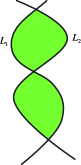
Figure 3. End 1

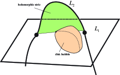
Figure 4. End 2

Remark 4.10.

Note in the case when the minimal Maslov number is $2$ we may have $k=2-2=0$. Since the (virtual) dimension of ${\mathcal{M}}(L_{1},L_{2};a,b;k,E^{\prime})$ is $k-1=-1$, one might imagine that this is enough to show that ${\mathcal{M}}(L_{1},L_{2};a,b;k,E^{\prime})$ is an empty set. However there is a case $a=b$. In that case ${\mathcal{M}}(L_{1},L_{2};a,a;0,0)$ consists of one point (the constant map $u$ to $a$). This is an element of ${\mathcal{M}}(L_{1},L_{2};a,a;0,0)$. So it is nonempty. Note this element is a fixed point of the ${\mathbb{R}}$ action. So even though the virtual dimension of ${\mathcal{M}}(L_{1},L_{2};a,a;0,0)$ is $-1$ it can still be nonempty. This is the reason why we need to assume that minimal Maslov index is strictly larger than $2$ in Theorem 4.4. This point is studied in great detail in [FOOO1, Section 3.6.3 etc.]. The notion of potential function introduced in [FOOO1, Definition 3.6.33] is related to this point.

As we have seen in this section, in the situation when the space $R(M;\mathcal{P}_{M})$ is embedded in $R(\partial M;\mathcal{P}_{\partial M})$ we can use its monotonicity to define Lagrangian Floer homology and prove Theorem 4.7.

In general $R(M;\mathcal{P}_{M})$ is an immersed Lagrangian submanifold in $R(\partial M;\mathcal{P}_{\partial M})$ even after making appropriate perturbation. However we still have a kind of monotonicity.

Definition 4.11.

Let $(X,\omega)$ be a symplectic manifold and $i_{L}:\tilde{L}\to X$ a Lagrangian immersion. Namely $i_{L}$ is an immersion, $\dim\tilde{L}=\frac{1}{2}\dim X$ and $i_{L}^{*}\omega=0$.

We say $L=(\tilde{L},i_{L})$ is monotone in the weak sense if for each pair $(u,\gamma)$ such that $u:D^{2}\to X$ and $\gamma:\partial S^{1}\to\tilde{L}$ with $u|_{\partial D^{2}}=i_{L}\circ\gamma$ the equality

$$\mu([u])=c\int_{D^{2}}u^{*}\omega$$ (4.9)

holds. (Note the Maslov index $\mu([u])$ can be defined in a similar way as embedded case.)

The minimal Maslov number is defined in the same way.

Proposition 4.12.

Let $(M,\mathcal{P}_{M})$ be a pair of an oriented 3 manifolds with boundary and a principal $SO(3)$ bundle on it such that $w^{2}(\mathcal{P}_{M})|_{\partial M}$ is the fundamental class $[\partial M]$. We also assume Assumption 2.2. Moreover we assume $R(M;\mathcal{P}_{M})\to R(\partial M;\mathcal{P}_{\partial M})$ is an immersion.

Then $R(M;\mathcal{P}_{M})$ is an immersed monotone Lagrangian submanifold in the weak sense. Its minimal Maslov number is congruent to $0$ modulo $4$.

However we cannot generalize Theorem 4.4 to the case of immersed monotone Lagrangian submanifold in the weak sense with minimal Maslov number $>2$. In fact other than those drawn in Figures 3 and 4 there exists another type of boundary of the moduli space ${\mathcal{M}}(L_{1},L_{2};a,b;2,E)$, which is drawn in Figure 5 below. So (4.4) does not hold in this generality.

Neverthless actually we can still define the right hand side of (4.5) and can prove the isomorphism (4.5). For this purpose we need various new ideas which was developped in Lagrangian Floer theory during 1996-2009. We describe some of them in the next section.

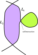
Figure 5. End 3

5. Biased review of Lagrangian Floer theory II

5.1. Filtered $A_{\infty}$ category

This subsection is a brief introduction to filtered $A_{\infty}$ category and algebra. For more detail, see [AFOOO, Fu10, Fu7, FOOO1, FOOO3, Ke, Le, Ly, Sei] and etc..

For the application to gauge theory such as Problem 2.1 we can work on ${\mathbb{Z}}$ or ${\mathbb{Z}}_{2}$ coefficient as we will explain in Subsection 6.1. However for the general story it is more natural to use universal Novikov ring which was introduced in [FOOO1]. We first define it below. Let $R$ be a commutative ring with unit, which we call ground ring. The reader may consider $R={\mathbb{Z}}_{2},{\mathbb{Z}},{\mathbb{R}}$ or ${\mathbb{C}}$. We take a formal variable $T$ and consider the formal sum

$$\sum_{k=0}^{\infty}a_{k}T^{\lambda_{k}}$$ (5.1)

such that:

1. $a_{k}\in R$.

2. $\lambda_{k}\in{\mathbb{R}}_{\geq 0}$.

3. $\lambda_{k}<\lambda_{k+1}$.

4. $\lim_{k\to\infty}\lambda_{k}=\infty$.

We call the totality of such formal sum (5.1) the universal Novikov ring and denote it by $\Lambda_{0}^{R}$. We replace (NR.2) by $\lambda_{k}\in{\mathbb{R}}$ (resp. $\lambda_{k}>{\mathbb{R}}$) to define $\Lambda^{R}$ (resp. $\Lambda_{+}^{R}$.) $\Lambda_{0}^{R}$ and $\Lambda^{R}$ become rings with unit in an obvious way. $\Lambda^{R}_{+}$ is an ideal of $\Lambda_{0}^{R}$. In case $R$ is a field, $\Lambda^{R}$ becomes a field, which we call (universal) Novikov field. In case $R$ is a field, $\Lambda^{R}_{+}$ is a maximal ideal of $\Lambda_{0}^{R}$. In fact $\Lambda_{0}^{R}/\Lambda_{+}^{R}=R$.

The ring $\Lambda^{R}$ has a filtration $F^{\lambda}\Lambda^{R}$ which consists of (5.1) with $a_{0}\geq\lambda$. It induces a filtration $F^{\lambda}\Lambda^{R}_{0}$ of $\Lambda^{R}_{0}$. This filtration defines a metric on these rings, by which they become complete.

Hereafter we omit $R$ and write $\Lambda_{0}$, $\Lambda$, $\Lambda_{+}$ in place of $\Lambda_{0}^{R}$, $\Lambda^{R}$, $\Lambda_{+}^{R}$, sometimes.

Definition 5.1.

A filtered $A_{\infty}$ category $\mathscr{C}$ consists of the following objects.

1. A set $\mathfrak{Ob}(\mathscr{C})$, which is the set of objects.

2. A graded $\Lambda_{0}$ module $\mathscr{C}(c_{1},c_{2})$ for each $c_{1},c_{2}\in\mathfrak{Ob}(\mathscr{C})$. We call $\mathscr{C}(c_{1},c_{2})$ the module of morphisms. It is a completion of a free $\Lambda_{0}$ module. (We may consider ${\mathbb{Z}}$ grading or ${\mathbb{Z}}_{2N}$ grading for some $N\in{\mathbb{Z}}_{>0}$. In our application in Section 6, we have ${\mathbb{Z}}_{4}$ grading. The number $2N$ in our geometric applications is a minimal Maslov number explained in the last section.)

3. For each $c_{0},\dots,c_{k}\in\mathfrak{Ob}(\mathscr{C})$, we are given operations ($\Lambda_{0}$ linear homomorphisms)

   $${\mathfrak{m}}_{k}:\mathscr{C}[1](c_{0},c_{1})\widehat{\otimes}\cdots\widehat{\otimes}\mathscr{C}[1](c_{k-1},c_{k})\to\mathscr{C}[1](c_{0},c_{k}),$$ (5.2)

   of degree $+1$ for $k=0,1,2,\cdots$ and $c_{i}\in\mathfrak{Ob}(\mathscr{C})$, which preserves the filtration. We call it structure operations. Here $\mathscr{C}[1](c,c^{\prime})$ is the degree shift of $\mathscr{C}(c,c^{\prime})$. Namely the degree $k$ part of $\mathscr{C}[1](c,c^{\prime})$ is degree $k+1$ part of $\mathscr{C}(c,c^{\prime})$. The symbol $\widehat{\otimes}$ denotes the $T$-adic completion of the algebraic tensor product.

4. The following $A_{\infty}$ relation is satisfied.

   $$0=\sum_{k_{1}+k_{2}=k+1}\sum_{i=0}^{k_{1}-1}(-1)^{*}\mathfrak{m}_{k_{1}}(x_{1},\dots,x_{i},\mathfrak{m}_{k_{2}}(x_{i+1},\dots,x_{k_{2}}),\dots,x_{k}),$$ (5.3)

   where $*=i+\sum_{j=1}^{i}\deg x_{j}$, $x_{i}\in\mathscr{C}[1](c_{i-1},c_{i})$, $c_{0},\dots,c_{k}\in\mathfrak{Ob}(\mathscr{C})$.

5. We require

   $$\mathfrak{m}_{0}(1)\equiv 0\mod T^{\epsilon},$$

   for some $\epsilon>0$.

6. An element ${\bf e}_{c}\in\mathscr{C}(c,c)$ of degree $0$ is given for each $c\in\mathfrak{Ob}(\mathscr{C})$ such that:

   1. If $x_{1}\in\mathscr{C}(c,c^{\prime})$, $x_{2}\in\mathscr{C}(c^{\prime},c)$ then

      $$\mathfrak{m}_{2}(\text{\bf e}_{c},x_{1})=x_{1},\quad\mathfrak{m}_{2}(x_{2},\text{\bf e}_{c})=(-1)^{\deg x_{2}}x_{2}.$$

   2. If $k+\ell\neq 1$, $x_{1}\otimes\dots\otimes x_{\ell}\in B_{\ell}\mathscr{C}[1](a,c)$, $y_{1}\otimes\dots\otimes y_{k}\in B_{k}\mathscr{C}[1](c,b)$ then

      $$\mathfrak{m}_{k+\ell+1}(x_{1},\cdots,x_{\ell},\text{\bf e}_{c},y_{1},\cdots,y_{k})=0.$$ (5.4)

      We call ${\bf e}_{c}$ the unit.

A filtered $A_{\infty}$ category with one object is called a filtered $A_{\infty}$ algebra.

A filtered $A_{\infty}$ category or algebra is called strict if $\mathfrak{m}_{0}=0$. It is called curved otherwise.

Note $\mathfrak{m}_{1}:\mathscr{C}(c,c^{\prime})\to\mathscr{C}(c,c^{\prime})$ is degree one and is regarded as a ‘boundary operator’. However in general $\mathfrak{m}_{1}\circ\mathfrak{m}_{1}=0$ does not hold. In fact (5.3) implies

$$\mathfrak{m}_{1}(\mathfrak{m}_{1}(x))+\mathfrak{m}_{2}(\mathfrak{m}_{0}(1),x)+(-1)^{\deg x+1}\mathfrak{m}_{2}(x,\mathfrak{m}_{0}(1))=0.$$ (5.5)

On the other hand (5.5) implies that $\mathfrak{m}_{1}\circ\mathfrak{m}_{1}=0$ if filtered $A_{\infty}$ category $\mathscr{C}$ is strict. The algebraic point about the well defined-ness of $\mathfrak{m}_{1}$ homology, which we mentioned above, is closely related to the geometric problem to define Lagrangian Floer theory, which we mentioned at the end of the last section. We will go back to this point in the next subsection.

An idea introduced in [FOOO1] is to deform Floer’s boundary operator $\mathfrak{m}_{1}$ to $\mathfrak{m}_{1}^{b}$ so that $\mathfrak{m}^{b}_{1}\circ\mathfrak{m}^{b}_{1}=0$ holds.

Definition 5.2.

Let $c\in\mathfrak{Ob}(\mathscr{C})$. A bounding cochain (or Maurer-Cartan element) of $c$ is an element $b\in\mathscr{C}(c,c)$ such that:

1. The degree of $b$ is $1$.

2. $b\equiv 0\mod\Lambda_{+}$.

3. $$\sum_{k=0}^{\infty}\mathfrak{m}_{k}(b,\dots,b)=0.$$ (5.6)

Note (2) implies that the left hand side of (5.6) converges in $T$ adic topology.

We denote by $\widetilde{\mathcal{M}}(c)$ the set of all bounding cochains. We say an object $c$ is unobstructed if $\widetilde{\mathcal{M}}(c)$ is nonempty.

Remark 5.3.

1. We can define appropriate notion of gauge equivalence among elements of $\widetilde{\mathcal{M}}(c)$. (See [FOOO1, Section 4.3].) The set of all gauge equivalence classes is called Maurer-Cartan moduli space and is written as ${\mathcal{M}}(c)$.

2. In certain situation we may relax the condition Definition 5.2 (2) and can use a class $b\in\mathscr{C}(c,c)$ of degreee $1$ which satisfies (5.6). (In such a case the left hand side of (5.6) should be defined carefully.) We write $\widetilde{\mathcal{M}}(c;\Lambda_{+})$ in place of $\widetilde{\mathcal{M}}(c)$ when we want to clarify that we consider only the elements satisfying Definition 5.2 (2).

Definition-Lemma 5.4.

Let $c,c^{\prime}\in\mathfrak{Ob}(\mathscr{C})$ and $b\in\widetilde{\mathcal{M}}(c)$, $b^{\prime}\in\widetilde{\mathcal{M}}(c^{\prime})$. We define

$$\mathfrak{m}_{1}^{b,b^{\prime}}:\mathscr{C}(c,c^{\prime})\to\mathscr{C}(c,c^{\prime})$$ (5.7)

by the formula:

$$\mathfrak{m}_{1}^{b,b^{\prime}}(x)=\sum_{k,\ell=0}^{\infty}\mathfrak{m}_{k+\ell+1}(\underbrace{b,\dots,b}_{k},x,\underbrace{b^{\prime},\dots,b^{\prime}}_{\ell}).$$ (5.8)

(5.3) and (5.6) imply

$$\mathfrak{m}_{1}^{b,b^{\prime}}\circ\mathfrak{m}_{1}^{b,b^{\prime}}=0.$$

We define

$$HF((c,b),(c^{\prime},b^{\prime}))=\frac{{\rm Ker}(\mathfrak{m}_{1}^{b,b^{\prime}}:\mathscr{C}(c,c^{\prime})\to\mathscr{C}(c,c^{\prime}))}{{\rm Im}(\mathfrak{m}_{1}^{b,b^{\prime}}:\mathscr{C}(c,c^{\prime})\to\mathscr{C}(c,c^{\prime}))}$$ (5.9)

and call it the Floer cohomology of $(c,b)$ and $(c^{\prime},b^{\prime})$.

We can deform $\mathfrak{m}_{k}$ in the same way as follows. Hereafter we write $\mathfrak{m}_{k+\ell+1}(b^{k},x,(b^{\prime})^{\ell})$ etc. in place of $\mathfrak{m}_{k+\ell+1}(\underbrace{b,\dots,b}_{k},x,\underbrace{b^{\prime},\dots,b^{\prime}}_{\ell})$ etc..

Definition-Lemma 5.5.

Let $\mathscr{C}$ be a curved filtered $A_{\infty}$ category. We define a strict filtered $A_{\infty}$ category $\mathscr{C}^{\prime}$ as follows.

1. An object of $\mathscr{C}^{\prime}$ is a pair $(c,b)$ where $c\in\mathfrak{OB}(\mathscr{C})$ and $b\in\widetilde{\mathfrak{M}}(c)$.

2. If $(c,b),(c^{\prime},b^{\prime})$ are objects of $\mathscr{C}^{\prime}$ then $\mathscr{C}^{\prime}((c,b),(c^{\prime},b^{\prime}))=\mathscr{C}(c,c^{\prime})$ by definition.

3. If $(c_{i},b_{i})\in\mathfrak{OB}(\mathscr{C}^{\prime})$ for $i=0,\dots,k$ and $x_{i}\in\mathscr{C}^{\prime}((c_{i-1},b_{i-1}),(c_{i},b_{i}))=\mathscr{C}(c_{i-1},c_{i})$ for $i=1,\dots,k$. Then we define the structure operations $\mathfrak{m}_{k}^{(b_{0},\dots,b_{k})}$ of $\mathscr{C}^{\prime}$ as follows.

   $$\mathfrak{m}_{k}^{(b_{0},\cdots,b_{k})}(x_{1},\cdots,x_{k})=\sum_{\ell_{0},\cdots,\ell_{k}}\mathfrak{m}_{k+\ell_{0}+\cdots+\ell_{k}}(b_{0}^{\ell_{0}},x_{1},b_{1}^{\ell_{1}},\cdots,b_{k-1}^{\ell_{k-1}},x_{k},b_{k}^{\ell_{k}}).$$ (5.10)

   We call $\mathscr{C}^{\prime}$ the associated strict category to $\mathscr{C}$.

Note

$$\mathfrak{m}_{0}^{(b)}(1)=\sum_{k=0}^{\infty}\mathfrak{m}_{k}(b,\dots,b)=0$$

by (5.6). We omit the proof that the structure operations (5.10) satisfies the relation (5.3), which is an easy calculation.

5.2. Immersed Lagrangian submanifold and its Floer homology

Let $i_{L}:\tilde{L}\to X$ be an $n$ dimensional immersed submanifold of a symplectic manifold $X$ of dimension $2n$. We say $L=(\tilde{L},i_{L})$ is an immersed Lagrangian submanifold if $i_{L}^{*}\omega=0$.

Definition 5.6.

We say that $L$ has clean self-intersection if the following holds.

1. The fiber product $\tilde{L}\times_{X}\tilde{L}$ is a smooth submanifold of $\tilde{L}\times\tilde{L}$.

2. For each $(p,q)\in\tilde{L}\times_{X}\tilde{L}$ we have

   $$\{(V,W)\in T_{p}\tilde{L}\oplus T_{q}\tilde{L}\mid di_{L}(V)=di_{L}(W)\}=T_{(p,q)}(\tilde{L}\times_{X}\tilde{L}).$$

We say $L$ has transversal self-intersection if

$$(\tilde{L}\times_{X}\tilde{L})\setminus\tilde{L}$$

is a finite set. (Note the fiber product $\tilde{L}\times_{X}\tilde{L}$ contains the diagonal $\cong\tilde{L}$.)

A finite set of immersed Lagrangian submanifolds $\{L_{i}\mid i=1,\dots,N\}$ is said a clean collection (resp. transversal collection) if the disjoint union $\bigcup_{i=1}^{N}L_{i}$ has clean self-intersection (resp. has transversal self-intersection).

Lagrangian Floer theory in [FOOO1, FOOO2] associates a filtered $A_{\infty}$ algebra to an embedded Lagrangian submanifold $L$. This $A_{\infty}$ algebra as a $\Lambda_{0}$ modle is taken to be the cohomology group of $L$ or any of its chain model. Namely it defines a homomorphism $\mathfrak{m}_{k}:H(L;\Lambda_{0})^{\otimes k}\to H(L;\Lambda_{0})$ satisfying (5.3). It also associates a filtered $A_{\infty}$ category ${\mathfrak{Fuk}}(\mathfrak{L})$ to a transversal collection of embedded Lagrangian submanifolds $\mathfrak{L}=\{L_{i}\mid i=1,\dots,N\}$ as follows.

1. The set of object is $\mathfrak{L}$.

2. For $L_{i},L_{j}\in\mathfrak{L}$, the module of morphisms, which we write $CF(L_{i},L_{j})$, is defined as follows:

   1. If $i\neq j$ then it is a free $\Lambda_{0}$ module whose basis is identified with $L_{i}\cap L_{j}$.

   2. If $i=j$ then $CF(L_{i},L_{i})=H(L_{i};\Lambda_{0})$.

3. The structure operations (5.2) is defined by using the moduli space of pseudoholomorphic $k+1$ gons.

Figure 6 below is the moduli space of $k+1$ gons, which calculate the coefficient of $[p]$ in $\mathfrak{m}_{7}(x_{1},\dots,x_{7}).$

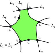
Figure 6. $\langle\mathfrak{m}_{7}(x_{1},\dots,x_{7}),x_{0}\rangle$

Akaho-Joyce [AJ] generalized this story to the immersed case as follows. Let $\mathfrak{L}$ be a transversal collection of immersed Lagrangian submanifolds $\mathfrak{L}=\{L_{i}\mid i=1,\dots,N\}$. Then we have a filtered $A_{\infty}$ category satisfying (L.C1)-(L.C3), except (L.C2) (2) is replaced by

1. If $i=j$ then

   $$CF(L_{i},L_{i})=H(L_{i};\Lambda_{0})\oplus\bigoplus\Lambda_{0}(p,q)$$ (5.11)

   where the direct sum is taken over all $(p,q)$ such that $i_{L_{i}}(p)=i_{L_{i}}(q)$ and $p\neq q$.

   We say $\bigoplus\Lambda_{0}(p,q)$ the switching part and $H(L_{i};\Lambda_{0})$ the diagonal part of $CF(L_{i},L_{i})$.

We remark that $(p,q)$ is an ordered pair. Namely $(p,q)\neq(q,p)$. So we associate extra two generators to each self-intersection.

The definition of structure operation including the generator $(p,q)$ is similar and by using the moduli space drawn below.

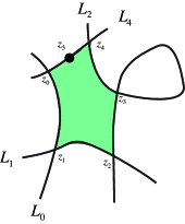
Figure 7. $\langle\mathfrak{m}_{7}(x_{1},\dots,x_{5}),x_{0}\rangle$

Note the 3rd marked point in the figure corresponds $(p,q)$ which is the extra generator appearing in item (2)’ above. Those generators correspond to the switchings at the boundary curve. We remark if $x=i_{L_{i}}(p)=i_{L_{i}}(q)$ is the self intersection point of $L_{i}$, the intersection $L_{i}\cap U$ of $L_{i}$ with a small neighborhood $U$ of $x$ consists of two smooth $n$ dimensional submanifolds. They are image of neighborhoods of $p$ and of $q$ respectively. Switching at 3rd marked point means that the boudary value was on one of the components of $L_{i}\cap U$ for $z\in\partial D^{2}$ $z<z_{3}$ and on the other component of $L_{i}\cap U$ for $z\in\partial D^{2}$ $z>z_{3}$. There are two different ways how the switching occurs. One is the switching from the component containing $p$ to the component containing $q$, and the other is the switching from the component containing $q$ to the component containing $p$. Those two different ways of switching correspond to the two generators appearing in (5.11).

5.3. The case of immersed Lagrangian submanifold which is monotone in the weak sense

Note (5.5) shows that the term $\mathfrak{m}_{0}(1)$ causes the problem to define Floer homology. Namely if $\mathfrak{m}_{0}(1)=0$ then $\mathfrak{m}_{1}\mathfrak{m}_{1}=0$. In other words we are looking for an appropriate element $b$ of $CF(L_{i},L_{i})$ such that $\mathfrak{m}^{b}_{0}(1)=0$. We called such $b$ a bounding cochain. The progress we made recently in our study of 3+2 dimensional Donaldson-Floer theory, is that we can now prove the existence of such $b$ in the situation appearing in it. We explain it in Section 6. Before doing so we go back to the situation of Subsection 4.2.

$\mathfrak{L}$ to a transversal collection of immersed Lagrangian submanifolds $\mathfrak{L}=\{L_{i}\mid i=1,\dots,N\}$.

Proposition 5.7.

Suppose each of $L_{i}$ are immersed monotone Lagrangian submanifolds in the weak sense and its minimal Maslov index is greater than $2$. Then the element

$$\mathfrak{m}_{0}(1)\in CF(L_{i},L_{i})$$

lies in the switching part.

Proof.

The diagonal part of $\mathfrak{m}_{0}(1)$ is defined as the (virtual) fundamental class of the moduli space of the pair $((D^{2},\partial D^{2}),z_{0}),u)$ where $u:(D^{2},\partial D^{2})\to(X,L_{i})$ is a pseudoholomorphic curve such that $\partial D^{2}\to L_{i}$ lifts to $\tilde{L}_{i}$. Therefore by assumption the (virtual) dimension of such modulie space is $\mu(\beta)+n-3+1$. Since $\mu(\beta)>2$ by assumption the dimension is greater than $n$. Hence it lines in $H_{*}(L_{i})$ with $*>n=\dim L_{i}$ and is $0$. ∎

By Proposition (5.7) and (5.5) the right hand side of

$$\mathfrak{m}_{1}\mathfrak{m}_{1}(x)=\mathfrak{m}_{2}(x,\mathfrak{m}_{0}(1))+\mathfrak{m}_{2}(\mathfrak{m}_{0}(1),x)$$

is defined by the moduli space as in Figure 5. In other words this formula is an algebraic way to explain the difficulty to define the Floer homology of a pair of immersed Lagrangian submanifolds which is monotone but immersed. (We explained it in Subsection 6 in a geometric way.)

We also have the following:

Proposition 5.8.

In the situation of Proposition 5.3 the sum appearing in the definition of structure operations are all finite sum and the construction works over the ground ring ${\mathbb{Z}}_{2}$ (or ${\mathbb{Z}}$ in the case when we can find orientations of the moduli space which is compatible at the boudnaries.).

The proof of the first half is similar to the proof of Proposition 5.7. The proof of the second half is similar to [FOOO4].

6. Instanton Floer homology for 3 manifolds with boundary

6.1. Main theorems

The next two theorems are the main results explained in this article. We assume the following for the simplicity of the statement. Let $M$ be a 3 manifold with boundary $\Sigma=\partial M$ and let $\mathcal{P}_{M}$ be a principal $SO(3)$ bundle. We denote $\mathcal{P}_{\Sigma}$ the restriction of $\mathcal{P}_{M}$ to $\Sigma$. We assume $w^{2}(\mathcal{P}_{\Sigma})=[\Sigma]$. (Assumption 1.1 (1).)

Assumption 6.1.

We assume Assumption 2.2. Moreover we assume that the restriction map defines an immersion $R(M;\mathcal{P}_{M})\to R(\Sigma;\mathcal{P}_{\Sigma})$.

We remark that we can reduce the general case to the case when this assumption is satisfied by perturbing the equation $F_{a}=0$ in the same way as [D1, Fl2, He].

Theorem 6.2.

We assume Assumption 6.1. Then the object $R(M;\mathcal{P}_{M})$ is unobstructed. Namely there exists a bounding cochain $b_{M}$ in $CF(R(M;\mathcal{P}_{M}))$.

Moreover we can find $b_{M}$ in a canonical way. In other words, its gauge equivalence class is an invariant of $(M;\mathcal{P}_{M})$.

Remark 6.3.

1. We omit the definition of gauge equivalence between bounding cochains. See [FOOO1, Definition 4.3.1].

2. We can remove Assumption 6.1 in Theorem 6.2 by perturbing the equation $F_{a}=0$ (which defines $R(M;\mathcal{P}_{M})$) on a compact subset of $M$. The same remark applies to the next theorem.

3. We can also prove that $b_{M}$ is supported in the switching components.

Theorem 6.4.

Suppose $(M_{1},\mathcal{P}_{M_{1}})$ and $(M_{2},\mathcal{P}_{M_{2}})$ satisfy Assumption 2.2. We also assume

$$\partial(M_{1},\mathcal{P}_{M_{1}})=(\Sigma,\mathcal{P}_{\Sigma}),\qquad\partial(M_{2},\mathcal{P}_{M_{2}})=(-\Sigma,\mathcal{P}_{\Sigma}).$$

We glue $(M_{1},\mathcal{P}_{M_{1}})$ and $(M_{2},\mathcal{P}_{M_{2}})$ along their boundaries to obtain $(M,\mathcal{P}_{M})$.

Then we have an isomorphism:

$$HF((R(M_{1};\mathcal{P}_{M_{1}}),b_{M_{1}}),(R(M_{2};\mathcal{P}_{M_{2}}),b_{M_{2}}))\cong HF(M,\mathcal{P}_{M})\otimes\Lambda_{0}^{{\mathbb{Z}}_{2}}.$$ (6.1)

Note the Lagrangian Floer homology in the left hand side has $\Lambda_{0}^{{\mathbb{Z}}_{2}}$ coefficient. However actually it can be defined over ${\mathbb{Z}}_{2}$ coefficient. In fact we have:

Proposition 6.5.

In the situation of Theorem 6.2 we may choose the bounding cochain $b_{M}$ so that it is entirely in the switching part.

Then using Proposition 5.8 we can define Floer homology

$$HF((R(M_{1};\mathcal{P}_{M_{1}}),b_{M_{1}}),(R(M_{2};\mathcal{P}_{M_{2}}),b_{M_{2}}))$$

over ${\mathbb{Z}}_{2}$ coefficient and (6.1) holds over ${\mathbb{Z}}_{2}$ coefficient.

Theorems 6.2 and 6.4 will be proved in a forthcoming joint paper with Alikebar Daemi.

6.2. A possible way to obtain bounding cochain $b_{M}$ directly from moduli spaces of ASD-connections

In this subsection we explain a conjecture which provides a way to obtain the bounding cochain $b_{M}$ in Theorem 6.2, directly by counting the order of certain moduli space of ASD-connections. The author is unable to prove this conjecture, which looks rather hard. The proof of Theorem 6.2 is performed in a different way as we will sketch in Subsections 6.3 and 6.4.

Let $(M,\mathcal{P}_{M})$ be as in Theorem 6.2. We consider the interior of $M$, that is $M\setminus\partial M$. We write it $M$ for simplicity of notation in this subsection. We choose its Riemannian metric such that $M$ minus a compact set is isometric to the direct product $\Sigma\times(0,\infty)_{t}$. We use $t$ as the coordinate of $(0,\infty)_{t}$. We put the suffix $t$ to clarify this point. We take direct product $M\times{\mathbb{R}}_{\tau}$ and use $\tau$ as the coordinate of ${\mathbb{R}}$ factor and consider a principal $SO(3)$ bundle $\mathcal{P}_{M}\times{\mathbb{R}}_{\tau}$.

Definition 6.6.

We consider the set of all connections $A$ of $\mathcal{P}_{M}\times{\mathbb{R}}_{\tau}$ with the following properties.

1. $F_{A}^{+}=0$. Namely $A$ is an Anti-Self-Dual connection.

2. We have

   $$\int_{M\times{\mathbb{R}}_{\tau}}\|F_{A}\|^{2}\,\,{\rm Vol}_{M}d\tau=E<\infty.$$ (6.2)

We denote by $\widetilde{\mathcal{M}}(M\times{\mathbb{R}}_{\tau};\mathcal{P}_{M}\times{\mathbb{R}}_{\tau};E)$ the set of all gauge equivalence classes of such $A$. (Here $E$ is as in (6.2).)

We can define an ${\mathbb{R}}_{\tau}$ action on $\widetilde{\mathcal{M}}(M\times{\mathbb{R}}_{\tau};\mathcal{P}_{M}\times{\mathbb{R}}_{\tau};E)$ by the translation of ${\mathbb{R}}_{\tau}$ direction. We denote by ${\mathcal{M}}(M\times{\mathbb{R}}_{\tau};\mathcal{P}_{M}\times{\mathbb{R}}_{\tau};E)$ the quotient space of this ${\mathbb{R}}$ action.

Conjecture 6.7.

We assume Assumption 6.1. Moreover we assume that $R(M;\mathcal{P}_{M})$ has transversal selfintersection. Then we can find an ${\mathbb{R}}_{\tau}$ invariant perturbation supported on a compact subset of $M$ so that the following holds.

1. $\mathcal{M}(M\times{\mathbb{R}}_{\tau};\mathcal{P}_{M}\times{\mathbb{R}}_{\tau};E)$ becomes a finite dimensional manifold.

2. We can compactify it so that the singularity of the compactification has codimension $4$.

3. Any element of $\mathcal{M}(M\times{\mathbb{R}}_{\tau};\mathcal{P}_{M}\times{\mathbb{R}}_{\tau};E)$ is gauge equivalent to a connection $A$ with the following properties.

   1. There exist $[a],[b]\in R(M;\mathcal{P}_{M})$ such that

      $$\lim_{\tau\to-\infty}A|_{M\times\{\tau\}}=a,\qquad\lim_{\tau\to+\infty}A|_{M\times\{\tau\}}=b.$$

   2. There exists $[\alpha]\in R(\Sigma;\mathcal{P}_{\Sigma})$ such that the following holds for any $\tau$.

      $$\lim_{t\to\infty}A|_{\Sigma\times\{(t,\tau)\}}=\alpha.$$

      Note we require $\alpha$ to be independent of $\tau$.

   3. In particular the restrction of $a$ and $b$ to $\Sigma$ are both gauge equivalent to $\alpha$.

4. If the dimension of $\mathcal{M}(M\times{\mathbb{R}}_{\tau};\mathcal{P}_{M}\times{\mathbb{R}}_{\tau};E)$ is zero then $[a]\neq[b]$ in item (3).

5. We put ${\rm Switch}=\{([a],[b])\mid[a]\neq[b],\,\,[a|_{\Sigma}]=[b|_{\Sigma}]\}$. For each $([a],[b])\in{\rm Switch}$ let $c([a],[b])$ be the number of elements $[A]$ as in item (3) such that it is in the zero dimensional component. Then the sum

   $$\sum_{([a],[b])\in{\rm Switch}}c([a],[b])([a],[b])\in CF(R(M;\mathcal{P}_{M}),R(M;\mathcal{P}_{M}))$$

   is the bounding cochain $b_{M}$ in Theorem 6.2.

This conjecture is difficult to prove. It seems that item (3) is a kind of Gauge theory analogue of a result by Bottman [Bo].

6.3. Right $A_{\infty}$ module and cyclic element

In this and the next subsections we explain a way to go around the difficult analysis to study the moduli space $\mathcal{M}(M\times{\mathbb{R}}_{\tau};\mathcal{P}_{M}\times{\mathbb{R}}_{\tau};E)$ but use an algebraic lemma to obtain the bounding cochain $b_{M}$. To state it we need a notations.

Definition 6.8.

Let $(C,\{\mathfrak{m}_{k}\})$ be a filtered $A_{\infty}$ algebra, which may be curved. A right filtered $A_{\infty}$ module over $(C,\{\mathfrak{m}_{k}\})$ is $(D,\{\mathfrak{n}_{k}\})$ such that:

1. $D$ is a graded $\Lambda_{0}$ module which is a completion of free $\Lambda_{0}$ module.

2. For $k=0,1,2,\dots$,

   $$\mathfrak{n}_{k}:D\otimes\underbrace{C[1]\otimes\cdots\otimes C[1]}_{k}\to D$$

   is a $\Lambda_{0}$ module homomorphism which preserves filtration and has degree $1$. Here $C[1]^{d}=C^{d+1}$ by definition.

3. The next relation holds for $y\in D$ and $x_{1},\dots,x_{k}\in C$.

   $$0= \sum_{\ell=0}^{k}\mathfrak{n}_{k-\ell}(\mathfrak{n}_{\ell}(y;x_{1},\dots,x_{\ell}),x_{\ell+1},\dots,x_{k}))$$ (6.3)

   $$+\sum_{i=-1}^{k}\sum_{j=i}^{k}(-1)^{*}\mathfrak{n}_{k-j+i+1}(y;x_{1},\dots,\mathfrak{m}(x_{i+1},\dots,x_{j}),x_{j+1},\dots,x_{k}),$$

   where $*=\deg y+\deg x_{1}+\dots+\deg x_{i}$.

Let $(D,\{\mathfrak{n}_{k}\})$ be a right filtered $A_{\infty}$ module over $(C,\{\mathfrak{m}_{k}\})$ and $b$ a bounding cochain of $(C,\{\mathfrak{m}_{k}\})$. We define $d^{b}:D\to D$ by

$$d^{b}(y)=\sum_{k=0}^{\infty}\mathfrak{n}_{k}(y;b,\dots,b).$$ (6.4)

It is easy to see from (6.3) that $d^{b}\circ d^{b}=0$.

Definition 6.9.

Let $(D,\{\mathfrak{n}_{k}\})$ be a right filtered $A_{\infty}$ module over $(C,\{\mathfrak{m}_{k}\})$. An element ${\bf 1}\in D$ is said to be a cyclic element if the following holds.

1. The map $x\mapsto\mathfrak{n}_{1}({\bf 1},x)$ is a $\Lambda_{0}$ module isomorphism: $C\to D$.

2. $\mathfrak{n}_{0}({\bf 1})\equiv 0\mod\Lambda_{+}$.

Definition 6.10.

Let $G$ be a submonoid of ${\mathbb{R}}$ which is discrete.

Let $C$ be a completion of a free $\Lambda_{0}$ module. An element $x$ of $C$ is said to be $G$-gapped if it is of the form

$$x=\sum_{i,j}a_{i,j}T^{\lambda_{i}}e_{j}$$

where $a_{i,j}\in R$ (the ground ring), $\lambda_{i}\in G\subset{\mathbb{R}}_{\geq 0}$, and $e_{j}$ is a basis of $C$.

Suppose $C_{i}$ ($i=1,2$) are completions of free $\Lambda_{0}$ modules. A filtered $\Lambda_{0}$ module homomorphism from $C_{1}$ to $C_{2}$ is said to be $G$-gapped if it sends $G$-gapped elements to $G$-gapped elements.

A filtered $A_{\infty}$ algebra (resp. category, module) are said to be $G$-gapped if all of its structure operations are $G$-gapped.

The filtered $A_{\infty}$ categories we obtain in Lagrangian Floer theory are always $G$-gapped for some $G$.

Proposition 6.11.

Let $(D,\{\mathfrak{n}_{k}\})$ be a right filtered $A_{\infty}$ module over $(C,\{\mathfrak{m}_{k}\})$. We assume that they are $G$-gappped. Let ${\bf 1}\in D$ be a cyclic element, which is also $G$-gapped.

Then there exists uniquely a $G$-gapped element $b$ of $C$ such that:

1. $b$ is a bounding cochain of $C$.

2. $$d^{b}({\bf 1})=0.$$ (6.5)

   Here $d^{b}$ is as in (6.4).

The proof is actually easy. We regard (6.5) as an equation for $b$. We can solve it by induction on energy filtration. (We use $G$-gapped-ness here so that the filtration is parametrized by a discrete set.) Then using $d^{b}(d^{b}({\bf 1}))=0$, we can show that $b$ is a bounding cochain. See [Fu9, Proposition 3.5] for the proof.

We remark that we do not assume that $C$ is unobstructed. Namely a priori there may not exist bounding cochain. In other words, we can use Proposition 6.11 to show the existence of bounding cochain. This turn out to be a useful tool to prove such existence. We remark that we are unable to define Lagrangian Floer homology unless we have some bounding cochain. So proving the existence of bounding cochain is a crucial step for various applications of Lagrangian Floer theory.

6.4. Existence of bounding cochain

In this subsection we show an outline of the way how we use Proposition 6.11 to prove Theorem 6.2.

To put the discussion in an appropriate perspective, we consider the following situation. Let $(M;\mathcal{P}_{M})$ be as in Theorem 6.2. Let $L$ be an immersed Lagrangian submanifold of $(\Sigma;\mathcal{P}_{\Sigma})$. We assume that $\{R(M;\mathcal{P}_{M}),L\}$ is a clean collection in the sense of Definition 5.6.

We put

$$CF((M;\mathcal{P}_{M});L)=C_{*}(R(M;\mathcal{P}_{M})\times_{(\Sigma;\mathcal{P}_{\Sigma})}L)\,\,\hat{\otimes}\,\,\Lambda_{0}.$$ (6.6)

Here $R(M;\mathcal{P}_{M})\times_{(\Sigma;\mathcal{P}_{\Sigma})}L$ is the fiber product of two immersed Lagrangian submanifolds and is a smooth manifold by our assumption. $C_{*}(R(M;\mathcal{P}_{M})\times_{(\Sigma;\mathcal{P}_{\Sigma})}L)$ is certain chain model of the homology group of this manifold. $\hat{\otimes}$ is the completion of algebraic tensor product.

Note $CF((M;\mathcal{P}_{M});L)$ as a $\Lambda_{0}$ module is the same as the underlying $\Lambda_{0}$ module $CF(R(M;\mathcal{P}_{M});L)$ of the chain complex which we use to define Floer homology $HF(R(M;\mathcal{P}_{M});L)$. We recall that we associated to $L$ a filtered $A_{\infty}$ algebra (as in Subsection 5.2). We write it $CF(L)$.

Theorem 6.12.

On $CF((M;\mathcal{P}_{M});L)$, there exists a structure of right filtered $A_{\infty}$ module over $CF(L)$.

We use the next proposition together with Theorem 6.12 to prove Theorem 6.2.

We take $L=R(M;\mathcal{P}_{M})$. Then by definition

$$CF((M;\mathcal{P}_{M});L)=C_{*}(R(M;\mathcal{P}_{M})\times_{R(\Sigma;\mathcal{P}_{\Sigma})}R(M;\mathcal{P}_{M}))\,\,\hat{\otimes}\,\,\Lambda_{0}.$$

We remark $R(M;\mathcal{P}_{M})$ is an open submanifold of $R(M;\mathcal{P}_{M})\times_{R(\Sigma;\mathcal{P}_{\Sigma})}R(M;\mathcal{P}_{M}))$. We denote by ${\bf 1}\in CF((M;\mathcal{P}_{M});R(M;\mathcal{P}_{M}))$ the differential $0$ form which is $1$ on $R(M;\mathcal{P}_{M})$ and is zero on other part.

Proposition 6.13.

${\bf 1}\in CF((M;\mathcal{P}_{M});R(M;\mathcal{P}_{M}))$ is a cyclic element of the right filtered $A_{\infty}$ module $CF((M;\mathcal{P}_{M});R(M;\mathcal{P}_{M}))$ over $CF(R(M;\mathcal{P}_{M}))$.

Theorem 6.2 is an immediate consequence of Proposition 6.11, Theorem 6.12 and Proposition 6.13.

In the rest of this subsection we briefly explain the idea of the proof of Theorem 6.12. The idea is to use Lagrangian submanifold $L$ as a boundary condition for an ASD-equation on $M\times{\mathbb{R}}$. (It appeared in [Fu2] in the year 1992. It is ellaborated in [Fu5]. Actually this is the motivation of the author when he introduced the notion of $A_{\infty}$ category in the study of gauge theory and of symplectic geometry.)

We put a metric on $M$ such that it is of product type $\Sigma\times(-1,0]$ near the neighborhood of the boundary $\partial M=\Sigma$. (Note this metric is different from one we used in Subsection 6.2. In Subsection 6.2 we take a Riemannian metric on $M\setminus\Sigma$ which is isometric to $\Sigma\times(0,\infty)$ outside a compact set.)

We then consider the product and $M\times{\mathbb{R}}_{\tau}$ and a connection $A$ on it such that:

1. $A$ is an ASD-connection. Namely $F_{A}^{+}=0$.

2. $$\int_{M\times{\mathbb{R}}_{\tau}}\|F_{A}\|^{2}{\rm Vol}_{M}d\tau<\infty.$$

3. There exists $(a,a^{\prime}),(b,b^{\prime})\in R(M;\mathcal{P}_{M})\times_{R(\Sigma;\mathcal{P}_{\Sigma})}L$ such that

   $$\lim_{\tau\to-\infty}A|_{M\times\{\tau\}}=a,\quad\lim_{\tau\to+\infty}A|_{M\times\{\tau\}}=b.$$

4. On $\partial M\times{\mathbb{R}}_{\tau}$ the connection $A$ satisfies a boundary condition determined by the Lagrangian submanifold $L$.

Remark 6.14.

The way how we write Condition (4) above is not precise. There are three different ways known to set this boundary conditions at the stage of 2016. (One which the author proposed in [Fu2] in the year 1992 does not seem to give a correct moduli space.)

1. The method to use a Riemannian metric which is degenerate near the boundary. This was introduced by the author in [Fu6] in 1997.

2. The method to require that $A$ is flat on each $\Sigma\times\{\tau\}$ and its gauge equivalence class is in $L$. This was introduced and used by Salamon-Wehrheim [SaWe, We1, We2] at the beginning of 21st century.

3. Using pseudoholomorphic curve equation near the boundary and a matching condition. This is introduced by Lipyanskiy [Ly1] around 2010.

The method (i), (iii) both can be used for our purpose. The compactness and removable singularity results which are needed for our purpose are proved in [Fu6] and in [Ly1]. The detail of the Fredholm theory is not yet written.

The method (ii) works for our purpose if $R(M;\mathcal{P}_{M})$ and $L$ are both embedded and monotone. In such a case [SaWe] gives a proof of Theorem 6.12. On the other hand it seems difficult to generalize this method beyond the case when $R(M;\mathcal{P}_{M})$ is embedded, by the reason explained in [Fu9, Section 6].

We consider the pair $(A,\vec{z})$ where $A$ is a connection on $M\times{\mathbb{R}}_{\tau}$ satisfying the above conditions (1)(2)(3)(4) and $\vec{z}=(\tau_{1},\dots,\tau_{k})\in{\mathbb{R}}_{\tau}$ with $\tau_{1}<\dots<\tau_{k}$. We denote the totality of (the gauge equivalence class of) such pair by $\mathcal{M}((M;\mathcal{P}_{M}),L)$. We use the boundary value of $A$ at $\Sigma\times\{\tau_{i}\}$ to define evaluation maps

$${\rm ev}=({\rm ev}_{1},\dots,{\rm ev}_{k}):\mathcal{M}((M;\mathcal{P}_{M}),L)\to(\tilde{L}\times_{R(\Sigma;\mathcal{P}_{\Sigma})}\tilde{L})^{k}.$$

We consider also the case when we switch at the marked point $z_{i}$. So the target space is as above. Using asymptotic limit as $\tau\to\pm\infty$ we obtain

$${\rm ev}_{\pm\infty}:\mathcal{M}((M;\mathcal{P}_{M}),L)\to R(M;\mathcal{P}_{M})\times_{R(\Sigma;\mathcal{P}_{\Sigma})}\tilde{L}.$$

Now let $h_{\pm\infty}$ is a differential form on $R(M;\mathcal{P}_{M})\times_{R(\Sigma;\mathcal{P}_{\Sigma})}\tilde{L}$ and $h_{1},\dots,h_{k}$ be differential forms on $\tilde{L}\times_{R(\Sigma;\mathcal{P}_{\Sigma})}\tilde{L}$. The right filtered $A_{\infty}$ module structure is defined roughly speaking by

$$\langle\mathfrak{n}_{k}([h_{-\infty}];[h_{1}],\dots,[h_{k}]),[h_{+\infty}]\rangle$$ (6.7)

$$=\int_{\mathcal{M}((M;\mathcal{P}_{M}),L)}{\rm ev}^{*}(h_{1}\times\dots h_{k})\wedge{\rm ev}_{-\infty}^{*}h_{-\infty}\wedge{\rm ev}_{+\infty}^{*}h_{+\infty}.$$

(Note we use integration in (6.7). When we work on ${\mathbb{Z}}_{2}$ coefficient we actually need to use, say, singular homology rather than de Rham homology.)

We can prove the relation (6.3) by studying the compactification of the moduli space $\mathcal{M}((M;\mathcal{P}_{M}),L)$ and its codimension one boundary.

6.5. Proof of Gluing theorem

In this subsection we sketch the proof of Theorem 6.4. This proof is a ‘gauge theory analogue’ of the proof by Lekili-Lipyanskiy [LL] of a similar result in Lagrangian correspondence. (See Section 7.)

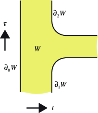
Figure 8. The domain $W$

We consider a domain $W$ of ${\mathbb{C}}$ as in Figure 8. It has three boundary components $\partial_{0}W$, $\partial_{1}W$, $\partial_{2}W$, which lie in the part $t=0$, $\tau<0$, $\tau>0$, respectively.

We consider the direct product $\Sigma\times W$ with the direct product metric. We glue $M_{1}\times{\mathbb{R}}_{\tau}$ with $W\times\Sigma$ by the diffeomorphism $\partial M_{1}\times{\mathbb{R}}_{\tau}\cong\Sigma\times\partial_{1}W$. We also glue $M_{2}\times{\mathbb{R}}_{\tau}$ with $W\times\Sigma$ by the diffeomorphism $\partial M_{2}\times{\mathbb{R}}_{\tau}\cong\Sigma\times\partial_{2}W$. We then obtain a 4 manifold $X$ with boundary and ends. $X$ has a boundary

$$\partial X=\Sigma\times\partial_{0}W\cong\Sigma\times{\mathbb{R}}_{\tau}.$$

$X$ has three ends.

1. $M_{1}\times(-\infty,0]_{\tau}$. This lies in the part where $\tau\to-\infty$.

2. $M\times[0,\infty)_{t}$. Here $M$ is obtained by gluing $M_{1}$ and $M_{2}$ along $\Sigma$. This lies in the part where $t\to\infty$.

3. $M_{1}\times[0,+\infty,0)_{\tau}$. This lies in the part where $\tau\to+\infty$.

See Figure 9.

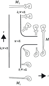
Figure 9. The 4 manifold $X$

Note the $SO(3)$-bundles $\mathcal{P}_{M_{1}}$ and $\mathcal{P}_{M_{2}}$ induce an $SO(3)$-bundle on $X$, which we denote by $\mathcal{P}_{X}$.

We take

$$\alpha,\beta\in R(M_{1};\mathcal{P}_{M_{1}})\times_{R(\Sigma;\mathcal{P}_{\Sigma})}R(M_{2};\mathcal{P}_{M_{2}}),$$

and consider the connection $A$ of $\mathcal{P}_{X}$ with the following properties.

1. $A$ is an ASD connection. Namely $F_{A}^{+}=0$.

2. On boundary $(-\infty,0]\times\Sigma$ we use the Lagrangian submanifold $R(M_{1};\mathcal{P}_{M_{1}})$ to set the boundary condition for $A$.

3. On boundary $[0,+\infty,0)\times\Sigma$ we use the Lagrangian submanifold $R(M_{2};\mathcal{P}_{M_{2}})$ to set the boundary condition for $A$.

4. At $\{(0,0)\}\times\Sigma$ we require that the restriction of $A$ is $\alpha$.

5. At the end (End.1) we require that $A$ is asymptotic to an element of

   $$R(M_{1};\mathcal{P}_{M_{1}})\subset R(M_{1};\mathcal{P}_{M_{1}})\times_{R(\Sigma;\mathcal{P}_{\Sigma})}R(M_{1};\mathcal{P}_{M_{1}}).$$

6. At the end (End.2) we require that $A$ is asymptotic to the flat connection $\beta$ of $(M,\mathcal{P}_{M})$.

7. At the end (End.3) we require that $A$ is asymptotic to an element of

   $$R(M_{2};\mathcal{P}_{M_{2}})\subset R(M_{2};\mathcal{P}_{M_{2}})\times_{R(\Sigma;\mathcal{P}_{\Sigma})}R(M_{2};\mathcal{P}_{M_{2}}).$$

8. $$\int_{X}\|F_{A}\|^{2}{\rm Vol}_{M}d\tau<\infty.$$

Note items (5) and (7) mean that $A$ is asymptotic to the cyclic element ${\bf 1}$ there. See Figure 10.

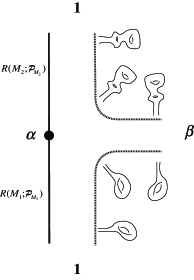
Figure 10. Condition for connection $A$

Definition 6.15.

We denote by $\mathcal{M}((X,\mathcal{P}_{X});\alpha,\beta)$ the moduli space of gauge equivalence classes of the connections $A$ satisfying the conditions (1)-(8) above.

We use this moduli space to define a map

$$CF((R(M_{1};\mathcal{P}_{M_{1}}),b_{M_{1}}),(R(M_{2};\mathcal{P}_{M_{2}}),b_{M_{2}}))\to CF(M;\mathcal{P}_{M})$$

by

$$[\alpha]\mapsto\sum_{\beta}\#\mathcal{M}((X,\mathcal{P}_{X});\alpha,\beta)[\beta].$$ (6.8)

Here we use the component of the moduli space $\mathcal{M}((X,\mathcal{P}_{X});\alpha,\beta)$ with (virtual) dimension $0$.

To show that (6.8) becomes a chain map, we study the compactification of $\mathcal{M}((X,\mathcal{P}_{X});\alpha,\beta)$ and show that its codimension one boundary is classified as follows.

1. The disk bubble at the boundary point $(\tau,0)$ with $\tau<0$.

2. Disk bubble at the boundary point $(\tau,0)$ with $\tau>0$.

3. Disk bubble at $(0,0)$.

4. Sliding ends as $\tau\to-\infty$.

5. Sliding ends as $\tau\to+\infty$.

6. Sliding ends as $t\to+\infty$.

See Figure 11.

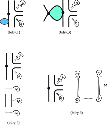
Figure 11. The boundary of $\mathcal{M}((X,\mathcal{P}_{X});\alpha,\beta)$

We can cancel the effect of the boundaries as in (bdry.1) and (bdry.2) using bounding cochains $b_{M_{1}}$ and $b_{M_{2}}$. (This part of the argument is the same as the Lagrangian Floer theory [FOOO1].) The effect of boudaries as in (bdry.4) and (bdry.5) is zero because of the equality

$$d^{b_{M_{1}}}{\bf 1}=d^{b_{M_{2}}}{\bf 1}=0.$$

(This is the equality (6.5), which we required when we defined $b_{M_{1}}$ and $b_{M_{2}}$.)

Therefore the remaining boundary components are ones of (bdry.3) and (bdry.6).

(bdry.3) is described by the sum of the product

$${\mathcal{M}}(R(M_{1};\mathcal{P}_{M_{1}}),R(M_{2};\mathcal{P}_{M_{2}});\alpha,\alpha^{\prime})\times\mathcal{M}((X,\mathcal{P}_{X});\alpha^{\prime},\beta)$$ (6.9)

for various $\alpha^{\prime}$. Here the first factor is a special case of the moduli space ${\mathcal{M}}(L_{1},L_{2};a,b)$, which we introduced in Subsection 4.1, using (LF.1),(LF.2),(LF.3).

(bdry.6) is described by the sum of the product

$$\mathcal{M}((X,\mathcal{P}_{X});\alpha,\beta^{\prime})\times{\mathcal{M}}(M\times{\mathbb{R}};\beta^{\prime},\beta)$$ (6.10)

for various $\beta^{\prime}$. Here the second factor is the moduli space introduced in Subsection 1.2 using condition (IF.1),(IF.2),(IF.3).

In the simplest case where $b_{M_{1}}=b_{M_{2}}=0$ the above argument implies that the sum of (6.9) and (6.10) is $0$ (in ${\mathbb{Z}}_{2}$ coefficient in our situation). It implies that the map (6.8) is a chain map.

In the general case we need additional term which is related to the correction by $b_{M_{i}}$. It is described by the moduli space drawn in Figure 12. (We omit the detail.)

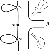
Figure 12. The correction to the map (6.8).

We again obtain a chain map

$$\mathscr{F}:CF((R(M_{1};\mathcal{P}_{M_{1}}),b_{M_{1}}),(R(M_{2};\mathcal{P}_{M_{2}}),b_{M_{2}}))\to CF(M;\mathcal{P}_{M}).$$

To show that $\mathscr{F}$ induces isomorphism we use energy filtration. The leading order term of the map $\mathscr{F}$ with respect to the energy filtration is the case of energy $0$. It consists of connections $A$ which is flat. In that case $\alpha$ is necessary equal to $\beta$. Thus the leading order term of the map $\mathscr{F}$ is the identity map, by using the identification

$$R(M_{1};\mathcal{P}_{M_{1}})\times_{R(\Sigma;\mathcal{P}_{\Sigma})}R(M_{2};\mathcal{P}_{M_{2}})\cong R(M;\mathcal{P}_{M}).$$

Therefore $\mathscr{F}$ induces the required isomorphism

$$HF((R(M_{1};\mathcal{P}_{M_{1}}),b_{M_{1}}),(R(M_{2};\mathcal{P}_{M_{2}}),b_{M_{2}}))\cong HF(M;\mathcal{P}_{M}).$$

This is the outline of the proof of Theorem 6.4.

7. Lagrangian correspondence and $A_{\infty}$ functors.

The story we described in Section 6 has an analogue in the study of Lagrangian correspondence, which we will outline in this section. See [Fu10] for detail. In this section we work over the ground ring ${\mathbb{R}}$. We need to take a spin or relative spin structure of a Lagrangian submanifold to use such ground ring. Spin or relative spin structures are necessary to orient the moduli spaces of pseudoholomorphic disks. (See [FOOO2, Chapter 8].) If $(X,\omega)$ is a symplectic manifold and $V$ is an oriented real vector bundle on it the $V$-relative spin structure of an oriented submanifold $L\subset X$ is by definition the spin structure of the bundle $TL\oplus V|_{L}$. Under this assumption the construction of Subsection 5.2 works over the ground ring ${\mathbb{R}}$ (or ${\mathbb{Q}}$).

7.1. The main results

Let $(X_{1},\omega_{1})$ and $(X_{2},\omega_{2})$ be compact symplectic manifolds.

Definition 7.1.

An immersed Lagrangian correspondence from $X_{1}$ to $X_{2}$ is an immersed Lagrangian submanifold of $(X_{1}\times X_{2},-\omega_{1}\oplus\omega_{2})$.

Let $L_{12}=(\tilde{L}_{12},i_{L_{12}})$ be an immersed Lagrangian correspondence from $X_{1}$ to $X_{2}$ and $L_{1}=(\tilde{L}_{1},i_{L_{1}})$ be an immersed Langrangian submanifold of $X_{1}$. If the fiber product $\tilde{L}_{2}=\tilde{L}_{1}\times_{X_{1}}\tilde{L}_{12}$ is transversal then, together with the composition $\tilde{L}_{1}\times_{X_{1}}\tilde{L}_{12}\to\tilde{L}_{12}\to X_{1}\times X_{2}\to X_{2}$, the manifold $\tilde{L}_{12}$ defines an immersed Lagrangian submanifold of $X_{2}$. We call it the geometric transformation of $L_{1}$ by $L_{12}$ and write it as $L_{1}\times_{X_{2}}L_{12}$.

Let $(X_{i},\omega_{i})$, $(i=1,2,3)$ be symplectic manifolds. Let $L_{12}$ be an immersed Lagrangian submanifold of $(X_{1}\times X_{2},-\omega_{1}\oplus\omega_{2})$ and $L_{23}$ a Lagrangian submanifold of $(X_{2}\times X_{3},-\omega_{2}\oplus\omega_{3})$. We assume that the fiber product

$$\tilde{L}_{12}\times_{X_{2}}\tilde{L}_{23}$$

is transversal and write the fiber product as $\tilde{L}_{13}$. Together with the obvious map $i_{L_{13}}:\tilde{L}_{13}\to X_{1}\times X_{3}$, the manifold $\tilde{L}_{13}$ defines an immersed Lagrangian submanifold $L_{13}$ of $(X_{1}\times X_{3},-\omega_{1}\oplus\omega_{3})$. We call $L_{13}$ the geometric composition of $L_{12}$ and $L_{23}$. We write it as $L_{12}\times_{X_{2}}L_{23}$.

See [We].

Definition 7.2.

The (immersed) Weinstein category is defined as follows. Its object is a symplectic manifold $(X,\omega)$. A morphism from $X_{1}$ to $X_{2}$ is an immersed Lagrangian correspondence from $X_{1}$ to $X_{2}$.

The composition of morphisms is defined as their geometric composition.

A slight issue is that, actually, we can define geometric composition only for a transversal pair. However, for the purpose of most of the applications, we can go around this problem by considering only composable pair of morphisms. In other words, Weinstein category is rather a ‘topological category’ where morphisms can be composed only on certain dense open subset. We can thus go around the problem by carefully stating various theorems in this subsection in such a way using only transversal pair for compositions. Another possible way to proceed is to introduce certain equivalence relation between Lagrangian submanifolds such as Hamiltonian isotopy or Lagrangian cobordism so that we can compose Lagrangian correspondences after perturbing them in the equivalence classes.

In Subsection 5.2 we start with a finite set of immersed Lagrangian submanifolds $\mathfrak{L}$ of $(X,\omega)$ (that is, a clean collection) and obtained a filtered $A_{\infty}$ category, the set of whose objects is $\mathfrak{L}$. We denote it by $\mathfrak{Fuk}(\mathfrak{L})$. Roughly speaking we can take ‘all’ immersed Lagrangian submanifolds and define $\mathfrak{Fuk}(X,\omega)$. An issue in doing so is perturbing all the Lagrangian submanifolds simultaneously to obtain some clean collection. We do not discuss this point. Using $\mathfrak{Fuk}(\mathfrak{L})$ instead of $\mathfrak{Fuk}(X,\omega)$ is enough for the purpose of most of the applications. To simplify the notation we pretend as if we defined the filtered $A_{\infty}$ category $\mathfrak{Fuk}(X,\omega)$. The actual result we prove is one which is restated by using $\mathfrak{Fuk}(\mathfrak{L})$ instead.

Note the filtered $A_{\infty}$ category $\mathfrak{Fuk}(X,\omega)$ is in general curved. We denote by $\mathfrak{Fuks}(X,\omega)$ the strict category associated to $\mathfrak{Fuk}(X,\omega)$.

In fact to take care of the problem of orientation and sign we need to use relative spin structure. We fix $V$ and consider a set of triples $(L,\sigma,b)$ where $L$ is a Lagrangian submanifold of $X$ and $\sigma$ is a $V$-relative spin structure and $b$ is a bounding cochain of $CF(L)$, that is the (curved) $A_{\infty}$ algebra obtained by using $(L,\sigma)$. The strict filtered $A_{\infty}$ category whose object is such triple $(L,\sigma,b)$ is abbreviated by $\mathfrak{Fuks}(X,\omega,V)$.

Definition 7.3.

An unobstructed immersed Weinstein category is defined as follows.

1. Its object is a triple $(X,\omega,V)$ where $(X,\omega)$ is a compact symplectic manifold and $V$ is a real oriented vector bundle on $X$.

2. A morphism from $(X_{1},\omega_{1},V_{1})$ to $(X_{2},\omega_{2},V_{2})$ is a triple $(L_{12},\sigma_{12},b_{12})$ where

   1. $L_{12}$ is an immersed Lagrangian submanifold of $(X_{1}\times X_{2},-\omega_{1}\oplus\omega_{2})$.

   2. $\sigma_{12}$ is a $\pi_{1}^{*}V_{1}\oplus\pi_{1}^{*}TX_{1}\oplus\pi_{2}^{*}V_{2}$- relative spin structure of $L_{12}$.

   3. $b_{12}$ is a bounding cochain of $CF(L_{12})$. (Note the filtered $A_{\infty}$ algebra $CF(L_{12})$ is defined by using the relative spin structure in (b).)

3. See Theorem 7.6 for the composition of the morphisms.

The main result of [Fu10] is a construction of the (2-)functor from the unobstructed immersed Weinstein category to the (2-)category of all filtered $A_{\infty}$ categories. We will state it as Theorems 7.4, 7.6, 7.7 below.

Theorem 7.4.

([Fu10]) Let $(L_{12},\sigma_{12},b_{12})$ be as in Definition 7.3 (2).

1. Let $(L_{1},\sigma_{1},b_{1})$ be an object of $\mathfrak{Fuks}(X_{1},\omega_{1},V_{1})$. Then the geometric transformation $L_{1}\times_{X_{1}}L_{12}$ has a canonical choice of $V_{2}$ relative spin structure $\sigma_{2}$ and a bounding cochain $b_{2}$.

2. There exists a strict filtered $A_{\infty}$ functor

   $$\mathfrak{W}_{L_{12}}:\mathfrak{Fuks}(X_{1},\omega_{1},V_{1})\to\mathfrak{Fuks}(X_{2},\omega_{2},V_{2})$$

   of which the map $(L_{1},\sigma_{1},b_{1})\mapsto(L_{1}\times_{X_{1}}L_{12},V_{2},b_{2})$ in item (1) is the object part.

3. There is a strict filtered $A_{\infty}$ bifunctor

   $$\mathfrak{Fuks}(X_{1}\times X_{2},-\omega_{1}\oplus\omega_{2},\pi_{1}^{*}V_{1}\oplus\pi_{1}^{*}TX_{1}\oplus\pi_{2}^{*}V_{2}) \times\mathfrak{Fuks}(X_{1},\omega_{1},V_{1})$$

   $$\to\mathfrak{Fuks}(X_{2},\omega_{2},V_{2})$$

   which induces $\mathfrak{W}_{L_{12}}$ when we fix an object of the first factor $\mathfrak{Fuks}(X_{1}\times X_{2},-\omega_{1}\oplus\omega_{2},\pi_{1}^{*}V_{1}\oplus\pi_{1}^{*}TX_{1}\oplus\pi_{2}^{*}V_{2})$.

The notions of filtered $A_{\infty}$ functor and bifunctor (and its strictness) are explained in the next subsection.

Remark 7.5.

If we assume all the Lagrangian submanifolds involved (including those appearing as fiber products among the Lagrangian submanifolds) are embedded, monotone and have minimal Maslov number $>2$, Theorem 7.4 follows from the earlier results by Wehrheim-Woodward [WW1, WW2] and Ma’u-Wehrheim-Woodwards [MWW]. The same remark applies to Theorems 7.6 and 7.7.

Note Theorem 7.4 (3) implies that there exists a strict filtered $A_{\infty}$ functor

$$\mathfrak{Fuks}(X_{1}\times X_{2},-\omega_{1}\oplus\omega_{2},\pi_{1}^{*}V_{1}\oplus\pi_{1}^{*}TX_{1}\oplus\pi_{2}^{*}V_{2})$$ (7.1)

$$\to\mathfrak{Funcs}(\mathfrak{Fuks}(X_{1},\omega_{1},V_{1}),\mathfrak{Fuks}(X_{2},\omega_{2},V_{2})).$$

Here $\mathfrak{Funcs}(\mathscr{C}_{1},\mathscr{C}_{2})$ is the strict filtered $A_{\infty}$ is category whose object is a strict filtered $A_{\infty}$ functor $:\mathscr{C}_{1}\to\mathscr{C}_{2}$.

Theorem 7.6.

([Fu10]) Let $(L_{12},\sigma_{12},b_{12})$ (resp. $(L_{23},\sigma_{23},b_{23})$) be morphisms from $(X_{1},\omega_{1},V_{1})$ to $(X_{2},\omega_{2},V_{2})$ (resp. from $(X_{2},\omega_{2},V_{2})$ to $(X_{3},\omega_{3},V_{3})$).

1. Let $L_{13}=L_{12}\times_{X_{2}}L_{23}$ be the geometric composition. Then we can define a $\pi_{2}^{*}V_{2}\oplus\pi_{2}^{*}TX_{2}\oplus\pi_{3}^{*}V_{3}$- relative spin structure $\sigma_{13}$ on it and a bounding cochain $b_{13}$ of $CF(L_{13})$. (In particular $L_{13}$ is unobstructed.)

2. Let $\mathfrak{W}_{L_{12}}$, $\mathfrak{W}_{L_{23}}$ and $\mathfrak{W}_{L_{13}}$ be strict filtered $A_{\infty}$ functors associated to $(L_{12},\sigma_{12},b_{12})$, $(L_{23},\sigma_{23},b_{23})$ and $(L_{13},\sigma_{13},b_{13})$, respectively, by Theorem 7.4 (2). Then

   $$\mathfrak{W}_{L_{23}}\circ\mathfrak{W}_{L_{12}}\sim\mathfrak{W}_{L_{13}}.$$ (7.2)

   Here the left hand side is the composition of strict filtered $A_{\infty}$ functors and $\sim$ is the homotopy equivalence of two strict filtered $A_{\infty}$ functors.

3. The next diagram commutes up to homotopy equivalence of strict filtered $A_{\infty}$ bifunctors.

   $$\begin{CD}\mathfrak{Fuks}(X_{1}\times X_{2})\times\mathfrak{Fuks}(X_{2}\times X_{3})@ >>>\mathfrak{Fuks}(X_{1}\times X_{3})\\ @ VVV@ VVV\\ \displaystyle\mathfrak{Funcs}(\mathfrak{Fuks}(X_{1}),\mathfrak{Fuks}(X_{2}))\atop\displaystyle\times\mathfrak{Funcs}(\mathfrak{Fuks}(X_{2}),\mathfrak{Fuks}(X_{3}))@ >>>\mathfrak{Funcs}(\mathfrak{Fuks}(X_{1}),\mathfrak{Fuks}(X_{3}))\end{CD}$$

   Here the vertical arrows are (7.1). (We omit the bundle $V_{i}$ in the notation.) The first horizontal line is a strict filtered $A_{\infty}$ bifunctor whose object part sends $((L_{12},\sigma_{12},b_{12}),(L_{23},\sigma_{23},b_{23}))$ to $(L_{13},\sigma_{13},b_{13})$ in item (1).

   The second horizontal line is a strict filtered $A_{\infty}$ bifunctor whose object part is a composition of filtered $A_{\infty}$ functors.

   (Note the commutativity of this diagram in the object level is (7.2).)

Theorem 7.7.

([Fu10]) The next diagram commutes up to homotopy equivalence of strict filtered $A_{\infty}$ tri-functors.

$$\begin{CD}\displaystyle\mathfrak{Fuks}(X_{1}\times X_{2})\times\mathfrak{Fuks}(X_{2}\times X_{3})\atop\displaystyle\!\!\!\!\!\!\!\!\!\!\!\!\!\!\!\!\!\!\!\!\!\!\!\!\!\!\!\!\!\!\!\!\!\!\!\!\!\!\!\!\!\!\times\mathfrak{Fuks}(X_{3}\times X_{4})@ >>>\mathfrak{Fuks}(X_{1}\times X_{3})\times\mathfrak{Fuks}(X_{3}\times X_{4})\\ @ VVV@ VVV\\ \mathfrak{Fuks}(X_{1}\times X_{2})\times\mathfrak{Fuks}(X_{2}\times X_{4})@ >>>\mathfrak{Fuks}(X_{1}\times X_{4}).\end{CD}$$

where all the arrows are defined by composition functor in Theorem 7.6.

Theorems 7.4, 7.6, 7.7 provide the functorial picture of the construction of $A_{\infty}$ categories out of symplectic manifolds.

Remark 7.8.

Theorems 7.4, 7.6, 7.7 provide the functorial picture up to the level of 2-category. Since the diagram in Theorem 7.7 commutes only up to homotopy, we may continue and may have a compatibility as $\infty$-categories.

7.2. $A_{\infty}$ functor, $A_{\infty}$ bi-functor, and Yoneda’s lemma

The proof of Theorem 6.2 which we explained in Subsection 6.4 could be regarded as a proof using the idea of representable functors. For the proof of Theorems 7.4, 7.6, 7.7 we use a similar idea in more systematic way. In this subsection we explain certain definitions and results in the story of $A_{\infty}$ category needed for this purpose. See [Fu7, Ke, Le, Ly, Sei] etc. for homological algebra of $A_{\infty}$ category. The notion of $A_{\infty}$ bi-functor is discussed in more detail in [Fu10].

Let $\mathscr{C}$ be an filtered $A_{\infty}$ category and $c,c^{\prime}\in\mathfrak{OB}(\mathscr{C})$. We define

$$B_{k}\mathscr{C}[1](c,c^{\prime})=\bigoplus\bigotimes_{i=1}^{k}\mathscr{C}[1](c_{i-1},c_{i})$$ (7.3)

where direct sum is taken over all $c_{0},\dots,c_{k}$ such that $c_{0}=c$ and $c_{k}=c^{\prime}$, and

$$B\mathscr{C}[1](c,c^{\prime})=\bigoplus_{k=0}^{\infty}B_{k}\mathscr{C}[1](c,c^{\prime}).$$ (7.4)

$B\mathscr{C}[1](c,c^{\prime})$ has a coalgebra structure

$$\Delta:B\mathscr{C}[1](c,c^{\prime})\to\bigoplus_{c^{\prime\prime}}B\mathscr{C}[1](c,c^{\prime\prime})\,\hat{\otimes}B\,\mathscr{C}[1](c^{\prime\prime},c^{\prime})$$

defined by

$$\Delta(x_{1}\otimes\dots\otimes x_{k})=\sum_{i=1}^{k-1}(x_{1}\otimes\dots\otimes x_{i})\otimes(x_{i+1}\otimes\dots\otimes x_{k}).$$

The operation $\mathfrak{m}_{k}$ induces a unique coderivation $B\mathscr{C}[1](c,c^{\prime})\to B\mathscr{C}[1](c,c^{\prime})$ so that its $Hom(B_{k}\mathscr{C}[1](c,c^{\prime}),B_{1}\mathscr{C}[1](c,c^{\prime}))$ component is $\mathfrak{m}_{k}$. We denote it by $\hat{d}_{k}$ and put

$$\hat{d}=\sum\hat{d}_{k}:B\mathscr{C}[1](c,c^{\prime})\to B\mathscr{C}[1](c,c^{\prime}).$$

The $A_{\infty}$ relation (5.3) is equivalent to the equality $\hat{d}\circ\hat{d}=0$.

Definition 7.9.

Let $\mathscr{C}_{1},\mathscr{C}_{2}$ be filtered $A_{\infty}$ categories. A filtered $A_{\infty}$ functor $\mathscr{F}:\mathscr{C}_{1}\to\mathscr{C}_{2}$ consists of objects:

1. A map $\mathscr{F}_{ob}:\mathfrak{OB}(\mathscr{C}_{1})\to\mathfrak{OB}(\mathscr{C}_{2})$.

2. A series of maps

   $$\mathscr{F}_{c,c^{\prime}}:B\mathscr{C}_{1}[1](c,c^{\prime})\to\mathscr{C}_{2}[1](\mathscr{F}_{ob}(c),\mathscr{F}_{ob}(c^{\prime})),$$

   which preserves filtrations.

3. We require that the coalgebra homomorphism

   $$\widehat{\mathscr{F}}_{c,c^{\prime}}:B\mathscr{C}_{1}[1](c,c^{\prime})\to B\mathscr{C}_{2}[1](\mathscr{F}_{ob}(c),\mathscr{F}_{ob}(c^{\prime}))$$

   induced by $\mathscr{F}_{c,c^{\prime}}$ is a chain map with respect to the boundary operator $\hat{d}$.

4. We require

   $$\widehat{\mathscr{F}}_{c,c^{\prime}}(x_{1},\dots,{\bf e},\dots,x_{k})=0$$

   except

   $$\widehat{\mathscr{F}}_{c,c}({\bf e}_{c})={\bf e}_{{\mathscr{F}}_{ob}(c)}.$$

A filtered $A_{\infty}$ functor is said to be strict if its restriction to $B_{0}\mathscr{C}_{1}[1](c,c)$ is $0$.

For a pair of filtered $A_{\infty}$ categories $\mathscr{C}_{1},\mathscr{C}_{2}$ we can define a filtered $A_{\infty}$ category $\mathfrak{Func}(\mathscr{C}_{1},\mathscr{C}_{2})$ whose object is a filtered $A_{\infty}$ functor $:\mathscr{C}_{1}\to\mathscr{C}_{2}$. We can define its strict version $\mathfrak{Funcs}(\mathscr{C}_{1},\mathscr{C}_{2})$ in the same way.

Definition 7.10.

Let $\mathscr{C}_{1},\dots,\mathscr{C}_{n}$ and $\mathscr{C}$ be filtered $A_{\infty}$ categories. A filtered $A_{\infty}$ multi-functor

$$\mathscr{F}:\mathscr{C}_{1}\times\dots\times\mathscr{C}_{n}\to\mathscr{C}$$

consists of the following objects.

1. A map $\mathscr{F}_{ob}:\prod_{i=1}^{n}\mathfrak{OB}(\mathscr{C}_{i})\to\mathfrak{OB}(\mathscr{C})$.

2. A series of $\Lambda_{0}$ module homomorphisms

   $$\mathscr{F}_{(c_{1},\dots,c_{n}),(c^{\prime}_{1},\dots,c^{\prime}_{n})}:\bigotimes_{i=1}^{n}B\mathscr{C}_{i}[1](c_{i},c_{i}^{\prime})\to\mathscr{C}(\mathscr{F}_{ob}(c_{1},\dots,c_{n}),\mathscr{F}_{ob}(c^{\prime}_{1},\dots,c^{\prime}_{n})),$$

   which preserve filtrations.

3. We require that the coalgebra homomorphism

   $$\hat{\mathscr{F}}_{(c_{1},\dots,c_{n}),(c^{\prime}_{1},\dots,c^{\prime}_{n})}:\bigotimes_{i=1}^{n}B\mathscr{C}_{i}[1](c_{i},c_{i}^{\prime})\to B\mathscr{C}[1](\mathscr{F}_{ob}(c_{1},\dots,c_{n}),\mathscr{F}_{ob}(c^{\prime}_{1},\dots,c^{\prime}_{n}))$$

   induced by ${\mathscr{F}}_{(c_{1},\dots,c_{n}),(c^{\prime}_{1},\dots,c^{\prime}_{n})}$ is a chain map with respect to the boundary operator $\hat{d}$.

4. $\hat{\mathscr{F}}_{(c_{1},\dots,c_{n}),(c^{\prime}_{1},\dots,c^{\prime}_{n})}(\bf x)$ is zero if $\bf x$ contains a unit except

   $$\hat{\mathscr{F}}_{(c_{1},\dots,c_{n}),(c_{1},\dots,c_{n})}({\bf e}_{c_{1}},\dots,{\bf e}_{c_{n}})={\bf e}_{\mathscr{F}_{ob}(c_{1},\dots,c_{n})}.$$

We use coalgebra structures of $B\mathscr{C}_{i}[1](c_{i},c_{i}^{\prime})$ to define a coalgebra structure on $\bigotimes_{i=1}^{n}B\mathscr{C}_{i}[1](c_{i},c_{i}^{\prime})$ in an obvious way.

We can define strictness of multi-functor in the same way.

Lemma 7.11.

The following two objects can be identified.

1. A filtered $A_{\infty}$ bifunctor $\mathscr{F}:\mathscr{C}_{1}\times\mathscr{C}_{2}\to\mathscr{C}$.

2. A filtered $A_{\infty}$ functor $\mathscr{F}:\mathscr{C}_{1}\to\mathfrak{Funk}(\mathscr{C}_{2},\mathscr{C})$.

Definition 7.12.

1. Let $\mathscr{C}$ be a strict filtered $A_{\infty}$ category and $c,c^{\prime}\in\mathfrak{OB}(\mathscr{C})$. We say $c$ and $c^{\prime}$ are homotopy equivalent if there exists $x\in\mathscr{C}(c,c^{\prime})$ and $x^{\prime}\in\mathscr{C}(c^{\prime},c)$ such that $\mathfrak{m}_{1}(x)=\mathfrak{m}_{1}(x^{\prime})=0$, $\mathfrak{m}_{2}(x,x^{\prime})-{\bf e}_{c}\in{\rm Im}(\mathfrak{m}_{1})$, $\mathfrak{m}_{2}(x^{\prime},x)-{\bf e}_{c^{\prime}}\in{\rm Im}(\mathfrak{m}_{1})$.

2. Two strict filtered $A_{\infty}$ functors $\mathscr{F}_{1},\mathscr{F}_{2}:\mathscr{C}_{1}\to\mathscr{C}_{2}$ are said to be homotopy equivalent each other if they are homopoty equivalent in the functor category $\mathfrak{Funcs}(\mathscr{C}_{1},\mathscr{C}_{2})$ in the sense of (1).

3. A strict filtered $A_{\infty}$ functor $\mathscr{F}:\mathscr{C}_{1}\to\mathscr{C}_{2}$ is said to be a homotopy equivalence if there exists a strict filtered $A_{\infty}$ functor $\mathscr{G}:\mathscr{C}_{2}\to\mathscr{C}_{1}$ such that the compositions $\mathscr{F}\circ\mathscr{G}$ and $\mathscr{G}\circ\mathscr{F}$ are homotopy equivalent to the identity functor.

Basic results in the story of $A_{\infty}$ category is the following two theorems.

Theorem 7.13.

(Whitehead theorem for $A_{\infty}$ functor) Let $\mathscr{F}:\mathscr{C}_{1}\to\mathscr{C}_{2}$ be a strict filtered $A_{\infty}$ functor between strict filtered $A_{\infty}$ categories. It is a homotopy equivalence if the following two conditions are satisfied.

1. For any $c^{\prime}\in\mathfrak{OB}(\mathscr{C}_{2})$ there exists $c\in\mathfrak{OB}(\mathscr{C}_{1})$ such that $\mathscr{F}_{ob}(c)$ is homotopy equivalent to $c^{\prime}$.

2. For any $c,c^{\prime}\in\mathfrak{OB}(\mathscr{C}_{1})$ the chain map

   $$\mathscr{F}_{c,c^{\prime}}:\mathscr{C}_{1}(c,c^{\prime})\to\mathscr{C}_{2}(\mathscr{F}_{ob}(c),\mathscr{F}_{ob}(c^{\prime}))$$

   is a chain homotopy equivalence.

We omit the proof. See [Fu7].

Let $\mathfrak{D}\subset\mathfrak{OB}(\mathscr{C})$. We define a filtered $A_{\infty}$ category whose object set is $\mathfrak{D}$ and the module of morphisms and structure operations are obvious restriction to those of $\mathscr{C}$. We call such a filtered $A_{\infty}$ category a full subcategory of $\mathcal{C}$.

We denote by $\mathscr{CH}$ an $A_{\infty}$ category whose object is a chain complex and whose module of morphisms between two chain complexes is the set of linear maps among them, which is a chain complex. The boundary operator of this chain complex is the operator induced from $\mathfrak{m}_{1}$ in an obvious way. The operation $\mathfrak{m}_{2}$ is the composition of linear maps (up to sign). $\mathfrak{m}_{3}$ and all higher $\mathfrak{m}_{k}$ are all zero.

Definition 7.14.

Let $\mathscr{C}$ be a filtered $A_{\infty}$ category. We define its opposite category $\mathscr{C}^{\rm op}$ as follows.

1. $\mathfrak{OB}(\mathscr{C}^{\rm op})=\mathfrak{OB}(\mathscr{C})$.

2. $\mathscr{C}^{\rm op}(c,c^{\prime})=\mathscr{C}(c^{\prime},c)$.

3. $$\mathfrak{m}^{\rm op}_{k}(x_{1},\dots,x_{k})=(-1)^{*}\mathfrak{m}_{k}(x_{k},\dots,x_{1})$$

   where $*=1+\sum_{1\leq i<j\leq k}(\deg x_{i}+1)(\deg x_{j}+1)$. Here $\mathfrak{m}^{\rm op}$ is the structure operation of $\mathscr{C}^{\rm op}$.

Theorem 7.15.

(Yoneda’s lemma for $A_{\infty}$ categories) Let $\mathscr{C}$ be a strict filtered $A_{\infty}$ category.

1. There exists a filtered $A_{\infty}$ functor $\mathfrak{YON}:\mathscr{C}\to\mathfrak{Funcs}(\mathscr{C}^{\rm op},\mathscr{CH}).$

2. Let $c\in\mathfrak{OB}(\mathscr{C})=\mathfrak{OB}(\mathscr{C}^{\rm op})$. Then $\mathfrak{YON}_{ob}(c):\mathfrak{OB}(\mathscr{C})\to\mathfrak{OB}(\mathscr{CH})$ is a strict filtered $A_{\infty}$ functor which is defined in the object level by

   $$c^{\prime}\mapsto\mathcal{C}(c,c^{\prime}).$$

3. Let $\mathfrak{Rep}(\mathscr{C}^{\rm op},\mathscr{CH})$ be a full subcategory of $\mathfrak{Funcs}(\mathscr{C}^{\rm op},\mathscr{CH})$, whose objects are elements of $\mathfrak{OB}(\mathfrak{Funcs}(\mathscr{C}^{\rm op},\mathscr{CH}))$ which is homotopy equivalent to the image of $\mathfrak{YON}_{ob}:\mathfrak{OB}(\mathfrak{\mathscr{C}})\to\mathfrak{OB}(\mathscr{C}^{\rm op},\mathscr{CH})$. Then

   $$\mathfrak{YON}:\mathscr{C}\to\mathfrak{Rep}(\mathscr{C}^{\rm op},\mathscr{CH}).$$

   is a homotopy equivalence.

We omit the proof. See [Fu7]. We call $\mathfrak{YON}$ the Yoneda functor. We say an element $\mathfrak{Rep}(\mathscr{C}^{\rm op},\mathscr{CH})$ a representable functor.

7.3. Künneth tri-functor and representability

In this subsection we sketch an argument to prove Theorem 7.4 using the algebraic framework of Subsection 7.2. Let $(L_{i},\sigma_{i})$ be a pair of Lagrangian submanifold of $X_{i}$ and its $V_{i}$-relative spin structure for $i=1,2$ and $(L_{12},\sigma_{12})$ a pair of Lagrangian submanifold of $(X_{1}\times X_{2},-\omega_{1}\oplus\omega_{2})$ and its $\pi_{1}^{*}V_{1}\oplus\pi_{1}^{*}TX_{1}\oplus\pi_{2}^{*}V_{2}$-relative spin structure. We consider curved filtered $A_{\infty}$ algebras $CF(L_{i})$ and $CF(L_{12})$. We assume appropriate transversality or clean-ness of intersection (or fiber product) among them.

Proposition 7.16.

There exists a left $CF(L_{1})$, $CF(L_{12})$ and right $CF(L_{2})$ filtered $A_{\infty}$ tri-mudule $D$ such that as a $\Lambda_{0}$ module $D$ is

$$H(\tilde{L}_{1}\times_{X_{1}}\tilde{L}_{12}\times_{X_{2}}\tilde{L}_{2};\Lambda_{0})$$

or its chain model.

The notion of tri-module is defined in a similar way as tri-functor (Definition 7.10). More explicitely it gives a series of operators

$$\mathfrak{n}_{k_{1},k_{12},k_{2}}:CF(L_{1})^{\otimes k_{1}}\otimes CF(L_{12})^{\otimes k_{12}}\otimes D\otimes CF(L_{2})^{\otimes k_{2}}\to D$$ (7.5)

which satisfies a smilar relation as right module. We sketch the proof of Proposition 7.16 later in this subsection.

Corollary 7.17.

If $b_{1}$ and $b_{12}$ are bounding cochains of $CF(L_{1})$ and $CF(L_{12})$ respectively then $D$ in Proposition 7.16 has a structure of right filtered $A_{\infty}$ module over $CF(L_{2})$.

Proof.

Using (7.5) we obtain

$$\mathfrak{n}_{k}:D\otimes CF(L_{2})^{\otimes k}\to D$$

by

$$\mathfrak{n}_{k}(y;x_{1},\dots,x_{k})=\sum_{k_{1},k_{12}=0}^{\infty}\mathfrak{n}_{k_{1},k_{12},k}(b_{1},\dots,b_{1};b_{12},\dots,b_{12};y;x_{1},\dots,x_{k}).$$

It is easy to check (6.3). ∎

Now we consider the case when $L_{2}$ is the geometric transformation $L_{1}\times_{X_{1}}L_{12}$. Then

$$D=H(\tilde{L}_{1}\times_{X_{1}}\tilde{L}_{12}\times_{X_{2}}\tilde{L}_{2};\Lambda_{0})=H(\tilde{L}_{2}\times_{X_{2}}\tilde{L}_{2};\Lambda_{0}).$$

The fundamental class of $\tilde{L}_{2}$ is an element of $D$, which we write ${\bf 1}$.

Lemma 7.18.

In the situation of Corollary 7.17 we assume that $L_{2}$ is the geometric transformation $L_{1}\times_{X_{1}}L_{12}$.

Then ${\bf 1}\in D$ is a cyclic element of right filtered $A_{\infty}$ module $D$.

Theorem 7.4 (1) is a consequence of Corollary 7.17, Lemma 7.18 and Proposition 6.11.

To prove Theorem 7.4 (2)(3) we enhance Proposition 7.16 as follows.

Proposition 7.19.

There exists a filtered $A_{\infty}$ tri-functor

$$\mathfrak{Fuks}(X_{1}\times X_{2},-\omega_{1}\oplus\omega_{2},\pi_{1}^{*}V_{1}\oplus\pi_{1}^{*}TX_{1}\oplus\pi_{2}^{*}V_{2})$$

$$\qquad\qquad\qquad\times\mathfrak{Fuks}(X_{1},\omega_{1},V_{1})\times\mathfrak{Fuks}(X_{2},\omega_{2},V_{2})^{\rm op}\to\mathscr{CH}$$

such that the chain complex associated to $L_{12}$, $L_{1}$, $L_{2}$ by this tri-functor is $D$ in Proposition 7.16.

By Proposition 7.19, Lemma 7.11 induces a bifunctor

$$\mathfrak{Fuks}(X_{1}\times X_{2},-\omega_{1}\oplus\omega_{2},\pi_{1}^{*}V_{1}\oplus\pi_{1}^{*}TX_{1}\oplus\pi_{2}^{*}V_{2})$$ (7.6)

$$\times\mathfrak{Fuks}(X_{1},\omega_{1},V_{1})\to\mathfrak{Funcs}(\mathfrak{Fuks}(X_{2},\omega_{2},V_{2})^{\rm op},\mathscr{CH}).$$

Proposition 7.20.

Let $(L_{1},\sigma_{1},b_{1})$ and $(L_{12},\sigma_{12},b_{12})$ be objects of $\mathfrak{Fuks}(X_{1},\omega_{1},V_{1})$ and $\mathfrak{Fuks}(X_{1}\times X_{2},-\omega_{1}\oplus\omega_{2},\pi_{1}^{*}V_{1}\oplus\pi_{1}^{*}TX_{1}\oplus\pi_{2}^{*}V_{2})$, respectively.

Then the strict filtered $A_{\infty}$ functor $:\mathfrak{Fuks}(X_{2},\omega_{2},V_{2})^{\rm op}\to\mathscr{CH}$ obtained by applying (7.6) to them is represented by the object $(L_{2},\sigma_{2},b_{2})$.

Here $L_{2}$ is the geometric composition and $b_{2}$ is obtained by Theorem 7.4 (1).

The proof is similar to the discussion in the next section using a diagram similar to the $Y$ diagram. See [Fu10].

By Proposition 7.20 we obtain a filtered $A_{\infty}$ bi-functor

$$\mathfrak{Fuks}(X_{1}\times X_{2},-\omega_{1}\oplus\omega_{2},\pi_{1}^{*}V_{1}\oplus\pi_{1}^{*}TX_{1}\oplus\pi_{2}^{*}V_{2})$$

$$\times\mathfrak{Fuks}(X_{1},\omega_{1},V_{1})\to\mathfrak{Rep}(\mathfrak{Fuks}(X_{2},\omega_{2},V_{2})^{\rm op},\mathscr{CH}).$$

Therefore we use Theorem 7.15 (3) and compose homotopy inverse to the Yoneda functor to obtain desired filtered $A_{\infty}$ functor in Theorem 7.4.

We finally sketch a proof of Proposition 7.16. We use the moduli space of objects drawn in the next Figure 13.

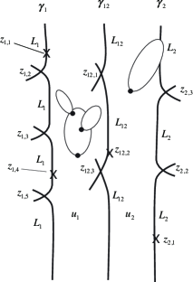
Figure 13. Moduli space of simple quilt

Here the source curve $\Sigma$ is the domain ${\mathbb{R}}_{\tau}\times[-1,1]_{t}$ plus possibly some sphere bubbles. We divide $\Sigma$ into two parts. The first one $\Sigma_{1}$ is the union of ${\mathbb{R}}_{\tau}\times[-1,0]_{t}$ and sphere bubbles rooted on it and the second one $\Sigma_{2}$ is the union of ${\mathbb{R}}_{\tau}\times[0,1]_{t}$ and sphere bubbles rooted on it. (We require the sphere bubbles are not rooted on the part $t=-1,0,1$.) The map is a combination of $u_{1}:\Sigma_{1}\to X_{1}$ and $u_{2}:\Sigma_{2}\to X_{2}$. We include three kinds of marked points $z_{1,1},\dots,z_{1,k_{1}}\in{\mathbb{R}}_{\tau}\times\{-1\}$, $z_{12,1},\dots,z_{12,k_{12}}\in{\mathbb{R}}_{\tau}\times\{0\}$, $z_{2,1},\dots,z_{2,k_{2}}\in{\mathbb{R}}_{\tau}\times\{1\}$.

We require the following boundary conditions:

1. $u_{1}(\tau,-1)\in L_{1}$.

2. $u_{2}(\tau,+1)\in L_{2}$.

3. $(u_{1}(\tau,0),u_{2}(\tau,0))\in L_{12}$.

4. $$\lim_{\tau\to-\infty}(u_{1}(\tau,t_{1}),u_{2}(\tau,t_{2}))=a\in\tilde{L}_{1}\times_{X_{1}}\tilde{L}_{12}\times_{X_{2}}\tilde{L}_{2}.$$

5. $$\lim_{\tau\to+\infty}(u_{1}(\tau,t_{1}),u_{2}(\tau,t_{2}))=b\in\tilde{L}_{1}\times_{X_{1}}\tilde{L}_{12}\times_{X_{2}}\tilde{L}_{2}.$$

Moreover we assume

1. $$\int_{\Sigma_{1}}u_{1}^{*}\omega_{1}+\int_{\Sigma_{2}}u_{2}^{*}\omega_{2}=E<\infty.$$

We denote the moduli space of such objects by $\mathcal{M}_{k_{1},k_{12},k_{2}}(L_{1},L_{12},L_{2};a,b;E)$. It comes with evaluation maps:

$${\rm ev}=({\rm ev}_{1},{\rm ev}_{12},{\rm ev}_{2}):\mathcal{M}_{k_{1},k_{12},k_{2}}(L_{1},L_{12},L_{2};a,b;E)\to\hat{L}_{1}^{k_{1}}\times\hat{L}_{12}^{k_{12}}\times\hat{L}_{2}^{k_{2}},$$

where

$$\hat{L}_{1}=\tilde{L}_{1}\times_{X_{1}}\tilde{L}_{1}.$$

$\hat{L}_{2}$ and $\hat{L}_{12}$ are defined in the same way.

Let $h_{i,j}$ $(j=1,\dots,k_{i})$ be differential forms on $\hat{L}_{i}$ and $h_{12,j}$ $(j=1,\dots,k_{12})$ differential forms on $\hat{L}_{12}$. Then we define the structure operations (7.5) of the tri-module $D$ by

$$\mathfrak{n}_{k_{1},k_{12},k_{2}}(\vec{h}_{1};\vec{h}_{12};[a];\vec{h}_{2})$$

$$=\sum_{E,b}T^{E}[b]\int_{\mathcal{M}_{k_{1},k_{12},k_{2}}(L_{1},L_{12},L_{2};a,b;E)}{\rm ev}^{*}(\vec{h}_{1}\wedge\vec{h}_{12}\wedge\vec{h}_{2}).$$

Here $\vec{h}_{1}=(h_{1,1},\dots,h_{1,k_{1}})\in CF(L_{1})^{\otimes k_{1}}$. The notations $\vec{h}_{12}$ and $\vec{h}_{2}$ are defined in a similar way.

We can show that it satisfies the required relation by studying the boundary of our moduli space $\mathcal{M}_{k_{1},k_{12},k_{2}}(L_{1},L_{12},L_{2};a,b;E)$ and using Stokes’ theorem.

We remark that our moduli space $\mathcal{M}_{k_{1},k_{12},k_{2}}(L_{1},L_{12},L_{2};a,b;E)$ is similar to one we use to define Floer homology group $HF(L_{1}\times L_{2},L_{12})$ in the product space $X_{1}\times-X_{2}$. For example in case $L_{1},L_{2},L_{12}$ are embedded and monotone with minimal Maslov number $>2$ we may use the case $k_{1}=k_{12}=k_{2}=0$ to obtain

$$\mathfrak{n}_{0,0,0}:D\to D$$

and $D$ is a free $\Lambda_{0}$ module with basis

$$L_{1}\times_{X_{1}}L_{12}\times_{X_{2}}L_{2}=(L_{1}\times L_{2})\cap L_{12}.$$

So $D$ is also the underlying vector space of the chain complex calculating Floer homology $HF(L_{1}\times L_{2},L_{12})$. Moreover the operation $\mathfrak{n}_{0,0,0}$ coincides with Floer’s boundary operator.

Remark 7.21.

To obtain appropriate Kuranishi structure we need to slightly change the way to compactify the bubble on the line $t=0$. (See [Fu10, Section 12].)

In case $k_{i}$ or $k_{12}$ are nonzero there is some technical difference between the moduli space $\mathcal{M}_{k_{1},k_{12},k_{2}}(L_{1},L_{12},L_{2};a,b;E)$ and the moduli space we use to define $CF(L_{1}\times L_{2})$-$CF(L_{12})$ bimodule structure on $D$.

Wehrheim-Woodward [WW1] studied the case of monotone Lagrangian submanifolds using the moduli space $\mathcal{M}_{0,0,0}(L_{1},L_{12},L_{2};a,b;E)$. They also generalize this moduli space to the case where the domain is divided into several (not necessary two) domains which are sent to various symplectic manifolds by a pseudoholomorphic curve. They call such objects pseudoholomorphic quilt. Here we use only the simplest case of pseudoholomorphic quilt.

7.4. Y diagram and compatibility of compositions

In this subsection we give a brief explanation of the proof of Theorem 7.6.

The proof of Theorem 7.6 (1) is similar to one of Theorem 7.4 (1). (In fact Theorem 7.4 (1) can be regarded as a special case of Theorem 7.6 (1) where $L_{3}$ is a point.) We construct a tri-module $D$ over $CF(L_{12})$, $CF(L_{23})$, $CF(L_{31})$ and use it in the same way as the last subsection. The moduli space we use for this purpose is obtained by replacing Figure 13 by the next Figure 14.

Figure 14. Composition of unobstructed correspondences

Here the source is a circular cylinder divided into three parts. The map is a combination of three maps $u_{1},u_{2},u_{3}$ which sends those three parts to $X_{1}$, $X_{2}$ and $X_{3}$ respectively. We use $L_{12}$, $L_{23}$, $L_{31}$ to set the boundary conditions at the lines where two of those three subdomains intersect. The underlying vector space of $D$ is the cohomology group of the triple fiber product

$$\left\{(x,y,z)\in\tilde{L}_{12}\times\tilde{L}_{23}\times\tilde{L}_{31}\,\,\left|\,\,\begin{aligned} &\pi_{1}(i_{L_{12}}(x))=\pi_{1}(i_{L_{31}}(z)),\\ &\pi_{2}(i_{L_{12}}(x))=\pi_{2}(i_{L_{23}}(z)),\\ &\pi_{3}(i_{L_{13}}(x))=\pi_{3}(i_{L_{23}}(z)).\end{aligned}\right\}\right.$$

Here $\pi_{i}:X_{i}\times X_{j}\to X_{i}$ and $\pi_{j}:X_{i}\times X_{j}\to X_{j}$ are projections.

We put elements of this triple fiber product at the part $\tau\to\pm\infty$ and use it as the asymptotic boundary condition.

The proof of Theorem 7.6 (2)(3) is based on the moduli space introduced by Lekili-Lipyanskiy [LL] which is drawn in the next Figure 15.

Figure 15. Lekili-Lipyanskiy’s Y-diagram

Here the source is a domain in ${\mathbb{C}}$ which is divided into three parts. The maps $u_{1},u_{2},u_{3}$ send each of those three parts to $X_{1}$, $X_{2}$, $X_{3}$, respectively and are pseudoholomorphic. Note in our situation of Theorem 7.6 (2)(3) we are given 6 Lagrangian submanifolds $L_{12}$, $L_{23}$, $L_{31}$, $L_{1}$, $L_{2}$, $L_{3}$, where $L_{i}\subset X_{i}$ and $L_{ij}\subset X_{i}\times X_{j}$. We use $L_{ij}$ to set the boundary condition at the curves where two subdomains intersect each other. We use $L_{i}$ to set the boundary condition at the boundary of our domain. We have six curves and so we put six kinds of marked points. The evaluation maps go to the products of $\hat{L}_{i}$’s and $\hat{L}_{ij}$’s.

Note our domain has 4 ends. Three of them (left, upper right and lower right) are similar to the ends appearing in Figure 13 and the fourth one which is a neighborhood of the white circle in the middle of the domain is similar to the end appearing in Figure 15.

Thus our moduli space defines a map which interpolates tensor products of $CF(L_{i})$, $CF(L_{ij})$ and tri-modules which we used to prove Theorem 7.6 (1) and Theorem 7.4 (1).

The $\Lambda_{0}$ linear maps we thus obtain looks rather cumbersome. However when we see them carefully we find that it is exactly the maps we need to show the homotopy commutativity of the diagrams appearing in Theorem 7.6 (2)(3). See [Fu10] for detail.

We finally mention that Theorem 7.7 is proved by using the objects drawn in the next Figure 16.

Figure 16. Associativity of compositions

8. Categorification of Donaldson-Floer theory

We can enhance the construction of Section 6 to the topological filed theory style results and clarify its relation to Lagrangian correspondence.

For oriented two manifold $\Sigma$ we always consider an $SO(3)$ bundle $E_{\Sigma}$ on it such that $w_{2}(E_{\Sigma})$ is the fundamental class. Let $R(\Sigma,E_{\Sigma})$ be the moduli space of the gauge equivalence classes of the flat connections of $E_{\Sigma}$. It is a symplectic manifolds and is monotone with minimal Chern number 2.

In this subsection we work over ${\mathbb{Z}}_{2}$ coefficient.

Definition 8.1.

We consider the strict filtered $A_{\infty}$ category $\mathfrak{Fuk}(\Sigma)$ as follows.

1. The object of $\mathfrak{Fuk}(\Sigma)$ is a pair $(L,b)$. Here $L$ is an immersed Lagrangian submanifold of $R(\Sigma,E_{\Sigma})$, which is monotone in the weak sense (Definition 4.11) and has minimal Maslov number divisible by $4$. $b$ is its bounding cochain which is supported in the switching components. (Here we consider the $\Lambda_{0}^{{\mathbb{Z}}_{2}}$ filtered $A_{\infty}$ algebra associated to $L$.)

2. The module of morphisms is $CF((L_{1},b_{1}),(L_{2},b_{2}))$ which is (${\mathbb{Z}}_{2}$ version) of the chain complex introduced in Subsection 4.1.

3. The structure operations $\mathfrak{m}_{k}$ is defined as in Subsection 5.2.

We remark that we can easily prove the following which is expected by topological field theory.

$$\mathfrak{Fuk}(\Sigma\sqcup\Sigma^{\prime})=\mathfrak{Fuk}(\Sigma)\otimes\mathfrak{Fuk}(\Sigma^{\prime}).$$ (8.1)

$$\mathfrak{Fuk}(-\Sigma)=\mathfrak{Fuk}(\Sigma)^{\rm op}.$$ (8.2)

Let $M$ be a 3 manifold with boundary $\Sigma=\partial M$. We consider an $SO(3)$ bundle $E_{M}$ on $M$ such that the restriction of $E_{M}$ to $\Sigma=\partial M$ is $E_{\Sigma}$. We assume that $\partial M$ is divided into $\partial_{-}M\sqcup\partial_{+}M$ such that a neighborhood of $\partial_{-}M$ (resp. a neighborhood of $\partial_{+}M$) in $M$ is identified with $\partial_{-}M\times[-\infty,0)$ (resp. $\partial_{+}M\times[0,+\infty)$) as oriented manifold.

By Theorem 6.2, the (appropriately perturbed) moduli space of flat connections $R(M;E_{M})$ is unobstructed. Namley we have a bounding cochain $b_{M}$ of the $\Lambda_{0}^{{\mathbb{Z}}_{2}}$ linear filtered $A_{\infty}$ algebra associated to $R(M;E_{M})\subset R(\Sigma_{-};E_{\Sigma_{-}})\times-R(\Sigma_{+};E_{\Sigma_{+}})$.

Definition 8.2.

Suppose $\Sigma_{-},\Sigma_{+}\neq\emptyset$. We define the strict filtered $A_{\infty}$ functor

$$\mathcal{HF}_{(M,E_{M})}:\mathfrak{Fuk}(\Sigma_{-})\to\mathfrak{Fuk}(\Sigma_{+})$$ (8.3)

as the strict filtered $A_{\infty}$ functor associated to the unobstructed immersed Lagrangian correspondence $(R(M;E_{M}),b_{M})$ by Theorem 7.4.

We can prove the following compatibility result. We consider $(M_{i},E_{M_{i}})$ ($i=1,2$) as above. We suppose $\partial_{+}M_{1}\cong\partial_{-}M_{2}$. We glue $M_{1}$ and $M_{2}$ along $\partial_{+}M_{1}\cong\partial_{-}M_{2}$ to obtain $M_{3}=M_{1}\#M_{3}$ and an $SO(3)$ bundle $E_{M_{3}}$ on it. Note

$$\partial_{-}M_{3}=\partial_{-}M_{1},\qquad\partial_{+}M_{3}=\partial_{+}M_{2}.$$

Theorem 8.3.

The filtered $A_{\infty}$ functor $\mathcal{HF}_{(M_{3},E_{M_{3}})}:\mathfrak{Fuk}(\partial_{-}M_{1})\to\mathfrak{Fuk}(\partial_{+}M_{2})$ associated to $(M_{3},E_{M_{3}})$ by Definition 8.2 is homotopy equivalent to the composition

$$\mathcal{HF}_{(M_{2},E_{M_{2}})}\circ\mathcal{HF}_{(M_{1},E_{M_{1}})}.$$

Here $\mathcal{HF}_{(M_{2},E_{M_{2}})}$, $\mathcal{HF}_{(M_{1},E_{M_{1}})}$ are filtered $A_{\infty}$ functors associated to $(M_{2},E_{M_{2}})$ and $(M_{1},E_{M_{1}})$ by Definition 8.2 and their composition is defined by Theorem 7.6 (1).

Definition 8.4.

Suppose $\Sigma_{-}=\emptyset,\Sigma_{+}\neq\emptyset$. Then we define $\mathcal{HF}_{(M,E_{M})}$ as the object $(R(M,E_{M}),b_{M})$ of $\mathfrak{Fuk}(\Sigma_{+})$.

Suppose $\Sigma_{-}\neq,\Sigma_{+}=\emptyset$. Then we define $\mathcal{HF}_{(M,E_{M})}$ as the filtered $A_{\infty}$ functor $:\mathfrak{Fuk}(\Sigma_{-})\to\mathcal{CH}$ which is represented by the object $(R(-M,E_{-M}),b_{-M})$ of $\mathfrak{Fuk}(\Sigma_{-})^{\rm op}$.

Suppose $\Sigma_{-}=\Sigma_{+}=\emptyset$. Then we define $\mathcal{HF}_{(M,E_{M})}$ as its Floer homology group as in Definition 1.6.

We can generalize Theorem 8.3 appropriately including the situation of Definition 8.4. Since this generalization is straightforward we omit it.

The proof of Theorem 8.3 uses the following Figure 17. $X$ in the figure is a 4 manifold. $X$ has 3 ends and 3 boundary components. The ends are identified with

$$M_{1}\times(-\infty,0],\qquad M_{2}\times(-\infty,0].\qquad M_{3}\times[0,+\infty,0).$$ (8.4)

The boundary (which are drawn by dotted lines) are identifies with

$$\partial_{-}M_{1}\times{\mathbb{R}}=\partial_{-}M_{2}\times{\mathbb{R}},\quad\partial_{+}M_{1}\times{\mathbb{R}}=\partial_{-}M_{2}\times{\mathbb{R}}\quad\partial_{+}M_{2}\times{\mathbb{R}}=\partial_{-}M_{3}\times{\mathbb{R}}.$$

The free domains $\Omega_{1}$, $\Omega_{2}$, $\Omega_{3}$ of ${\mathbb{C}}$ are attached to each of such boundary components. We consider an Anti-Self-Dual connection $A$ on $X$ and holomorphic maps $u_{1}:\Omega_{1}\to R(\partial_{-}M_{1})$, $u_{2}:\Omega_{2}\to R(\partial_{-}M_{2})$, $u_{3}:\Omega_{3}\to R(\partial_{+}M_{3})$.

Along three dotted lines we require appropriate matching condition similar to those in [Fu6, Ly1]. We also require $u_{1}$, $u_{2}$, $u_{3}$ satisfy appropriate boundary condition on $\partial\Omega_{i}\setminus\text{\rm dotted lines}$, formulated by using Lagrangian submanifolds $R(M_{1};E_{M_{1}})$, $R(M_{2};E_{M_{2}})$, $R(M_{3};E_{M_{4}})$, respectively.

We consider the moduli space of the such triples $(A,u_{1},u_{2},u_{3})$. (We also include boundary marked points on the $\partial\Omega_{i}\setminus\text{\rm dotted lines}$ and require certain asymptotic boundary conditions on the three ends.)

We observe the sliding ends of this moduli space corresponding to the three ends in (8.4) coincide with the moduli spaces we use to obtain bounding cochain $b_{M_{1}}$, $b_{M_{2}}$, $b_{M_{3}}$, respectively.

Using the moduli space of the triples $(A,u_{1},u_{2},u_{3})$ (plus marked points), we can show that $b_{M_{1}}$, $b_{M_{2}}$, $b_{M_{3}}$ satisfies certain equalities which is the one we need to prove Theorem 8.3.

In this article we restrict ourselves to the case of $SO(3)$ bundles $E$ with nontrivial $w_{2}(E)$. The research to include the case when $E$ is a trivial bundle is now in progress. See [DF].

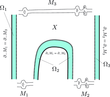
Figure 17. Proof of Theorem 8.3

Acknowledgement. The research of the author is supported partially by NSF Grant No. 1406423 and Simons Collaboration for homological Mirror symmetry.

References

- [AFOOO] M. Abouzaid, K. Fukaya, Y.-G. Oh, H. Ohta and K. Ono, Quantum cohomology and split generation in Lagrangian Floer theory, in preparation.
- [Ak] M. Akaho, Intersection theory for Lagrangian immersions, Math. Res. Lett. 12 (2005), 543–550.
- [AJ] M. Akaho and D. Joyce, Immersed Lagrangian Floer theory, J. Differential Geometry 86 (2010) 381-500.
- [At] M.F. Atiyah, New invariants of three and four dimensional manifolds, Proc. Symp. Pure Math. 48 (1988).
- [AB] M. F. Atiyah and R. Bott, The Yang Mills equations over Riemann surfaces, Philos. Trans. Roy. Soc. London A 308 (1982) 523–615
- [Bo] N. Bottman, Pseudoholomorphic quilts with figure eight singularity, arXiv:1410.3834.
- [BW] N. Bottman and K. Wehrheim, Gromov compactness for squiggly strip shrinking in pseudoholomorphic quilts, arXiv:1410.3834.
- [BD] D. Braam and S. Donaldson, Floer’s work on instanton homology, knots, and surgery, in Floer Memorial Volume, Hofer, Zender, and Taubes, Editors. 1995, Birkhäuser. pp. 195–256.
- [DF] A. Daemi and K. Fukaya Atiyah-Floer Conjecture: a Formulation, a Strategy to Prove and Generalizations, in preparation.
- [DFL] A. Daemi, K. Fukaya and M. Lipyanskiy, Lagrangians, -instantons, and an Analogue of Atiyah-Floer Conjecture, in preparation.
- [D1] S. Donaldson, The orientation of Yang-Mills moduli spaces and 4-manifold topology, J. Differential Geometry 26 (1987) 397–428.
- [D2] S. Donaldson, Connections, cohomology and the intersection forms of 4-manifolds, J. Differential Geom. Volume 24, Number 3 (1986), 275-341.
- [D3] S. Donaldson, Polynomial invariants for smooth four-manifolds, Topology 29 (1990), no. 3, 257–315.
- [D4] S. Donaldson, Gauge theory for non-athlete, Lecture at University of Warwick, 1992.
- [D5] S. Donaldson, Floer homology groups in Yang-Mills theory. With the assistance of M. Furuta and D. Kotschick. Cambridge Tracts in Mathematics, 147. Cambridge University Press, Cambridge, 2002. viii+236
- [DS] S. Dostoglou and D.A. Salamon, Self-dual instantons and holomorphic curves, Annals of Mathematics 139 (1994), 581–640.
- [Fl1] A. Floer Morse theory for Lagrangian intersections, J. Differential Geom. 28 (1988) 513–547
- [Fl2] A. Floer, Instanton invariant for 3-manifolds, Comm. Math. Phys. 118 (1988), 215–240.
- [Fl3] A. Floer, Instanton homology and Dehn surgery, in Floer Memorial Volume, Hofer, Zender, and Taubes, Editors. 1995, Birkhäuser. pp. 77–98.
- [Fl4] A. Floer, Instanton invariants for knots, in Floer Memorial Volume, Hofer, Zender, and Taubes, Editors. 1995, Birkhüser. p. 99–104.
- [Fu1] K. Fukaya, Morse homotopy, -Category, and Floer homologies, in “Proceedings of Garc Workshop on Geometry and Topology” ed. by H.J. Kim, Seoul National University (1994), 1-102.
- [Fu2] K. Fukaya, Floer homology for 3-manifolds with boundary -abstract -, in ‘Topology Geometry and Field theory’ ed by Fukaya, Furuta, Khono, Kotchick, World Scientific, Singapore (1994), 1-22.
- [Fu3] K. Fukaya, Gauge theory and topology , Springer Tokyo, 1995 (in Japanese).
- [Fu4] K. Fukaya, Floer homology of connected sum of homology 3-spheres, Topology 35 (1996) 88–136.
- [Fu5] K. Fukaya, Floer homology for 3-manifolds with boundary I (1997), never to be published but is available at http://www.math.kyoto-u.ac.jp/%7Efukaya/fukaya.html.
- [Fu6] K. Fukaya, Anti-Self-Dual equation on 4-manifolds with degenerate metric, Geometric Analysis and Functional Analysis 8 (1998) 466–528.
- [Fu7] K. Fukaya, Floer homology and mirror symmetry II, Minimal Surfaces, Geometric Analysis and Symplectic Geometry (Baltimore, MD, 1999), Adv. Stud. Pure Math. 34 (2002), 31–127.
- [Fu8] K. Fukaya Floer homology of Lagrangian submanifolds. Sugaku Expositions 26 (2013), no. 1, 99–127.
- [Fu9] K. Fukaya, -Floer homology of 3 manifolds with boundary 1, preprint, arXiv:1506.01435.
- [Fu10] K. Fukaya, Unobstructed Lagrangian correspondence and functor, in preparation.
- [FOOO1] K. Fukaya, Y.-G. Oh, H. Ohta and K. Ono, Lagrangian intersection Floer theory-anomaly and obstruction, Part I, AMS/IP Studies in Advaneced Math. vol. 46.1, International Press/ Amer. Math. Soc. (2009). MR2553465.
- [FOOO2] K. Fukaya, Y.-G. Oh, H. Ohta and K. Ono, Lagrangian intersection Floer theory-anomaly and obstruction, Part II, AMS/IP Studies in Advanced Math. vol. 46.2, International Press/ Amer. Math. Soc. (2009). MR2548482.
- [FOOO3] K. Fukaya, Y.-G. Oh, H. Ohta and K. Ono, Anchored Lagrangian submanifolds and their Floer theory. in ‘Mirror symmetry and tropical geometry’, 15-54, Contemp. Math., 527, Amer. Math. Soc., Providence, RI, (2010).
- [FOOO4] K. Fukaya, Y.-G. Oh, H. Ohta and K. Ono, Lagrangian Floer theory over integers: spherically positive symplectic manifolds, Pure and Applied Mathematics Quaterly Volume 9, Number 2 189–289 (2013), arXiv:1105.5124.
- [FOOO5] K. Fukaya, Y.-G. Oh, H. Ohta and K. Ono, Kuranishi structure, Pseudo-holomorphic curve, and Virtual fundamental chain: Part 1, arXiv:1503.07631.
- [FOOO6] K. Fukaya, Y.-G. Oh, H. Ohta and K. Ono, Kuranishi structure, Pseudo-holomorphic curve, and Virtual fundamental chain: Part 2, in preparation.
- [FOn] K. Fukaya and K. Ono, Arnold conjecture and Gromov-Witten invariant, Topology 38 (1999), no. 5, 933–1048.
- [Go] W. Goldman, The symplectic nature of fundamental groups of surfaces. Adv. in Math. 54 (1984), no. 2, 200–225.
- [He] C. Herald, Legendrian cobordism and Chern-Simons theory on 3-manifolds with boundary, Comm. Anal. Geom., 2 (1994) 337–413.
- [Hu] J. Huebchmann, Symplectic and Poisson structures of certain moduli spaces. I, Duke Math. J. 80(3) (1995) 737–756.
- [HL] D. Huybrechts and M. Lehn Stable pairs on curves and surfaces arXiv:alg-geom/9211001. J. Algebraic Geom. 4 (1995) 67–104.
- [Je] L. Jeffrey Extended moduli space of flat connections on Riemann surfaces, Math. Ann. 298 (1994) 667-692.
- [Ke] B. Keller, Introduction to A-infinity algebra and modules, Homology Homotopy Appl. 3 (2001) no 1-35 (electoric). 340.
- [LL] Y. Lekili and M. Lipyanskiy, Geometric composition in quilted Floer theory, Adv. Math. 236 (2013), 1–23.
- [LLW] R. Lee and W. Li, Floer homologies for Lagrangian intersections and instantons, preprint.
- [Le] K. Lefèvre-Hasegawa, Sur les catégories, Thése Doctorat Universite Paris 7 (2003).
- [Li] W. Li, Floer homology for connected sums of homology 3-spheres, J. Differential Geom. 40 (1994) 129–154.
- [LOT] R. Lipshitz, P.S. Ozsvath and D. Thurston, A tour of bordered Floer theory, Proc. Nat. Acad. Sci. 108 (2011) 8085–8092.
- [Ly1] M. Lipyanskiy, Gromov-Uhlenbeck Compactness, arXiv:1409.1129.
- [Ly2] M. Lipyanskiy, Gromov-Uhlenbeck Compactness and the Atiyah-Floer Conjecture, talk at SCGP 2012-09-25, video is available at SCGP home page.
- [Lu] J. Lurie On the Classification of Topological Field Theories (Draft), preprint, arXiv:0905.0465v1.
- [Ly] V. Lyubashenko, Category of -categories, Homotopy and Applications 5 (2003), 1–48.
- [MW] C. Manolescu and C. Woodward, Floer homology on the extended moduli space, Perspective in analysis, geometry, and topology, 283–329, Progre. Math. 296, Birkhäuser, New York.
- [MWW] S. Ma’u, K. Wehrheim and C. Woodward, -functor for Lagrangian correspondences, preprint.
- [Oh] Y.-G. Oh, Floer cohomology of Lagrangian intersections and pseudo-holomorphic disks I, II, Comm. Pure and Appl. Math. 46 (1993), 949–994, 995–1012; Addenda, ibid, 48 (1995), 1299 –1302.
- [Sa] D. Salamon, Lagrangian intersections, 3-manifolds with boundary, and the Atiyah-Floer conjecture, Proceedings of the ICM, Zürich 1994, Vol. 1, 526–536.
- [SaWe] D. Salamon and K. Wehrheim, Instanton Floer homology with Lagrangian boundary conditions, Geom. Topol. 12 (2008), no. 2, 747–918.
- [Se1] G. Segal, The definition of conformal field theory. Differential geometrical methods in theoretical physics (Como, 1987), 165–171, NATO Adv. Sci. Inst. Ser. C Math. Phys. Sci., 250, Kluwer Acad. Publ., Dordrecht, 1988.
- [Se2] G. Segal, Geometric aspects of quantum field theory. Proceedings of the International Congress of Mathematicians, Vol. I, II (Kyoto, 1990), 1387–1396, Math. Soc. Japan, Tokyo, 1991.
- [Sei] P. Seidel, Fukaya categories and Picard-Lefschetz theory, Zürich Lectures in Advanced Mathematics. European Mathematical Society (EMS), Zr̈ich, 2008. viii+326 pp.
- [We1] K. Wehrheim, Anti-self-dual instantons with Lagrangian boundary conditions I: Elliptic theory II : Bubbling, Comm. Math. Phys. 254 (2005), no. 1, 45–89, ibid. 258 (2005), no. 2, 275–315.
- [We2] K. Wehrheim, Lagrangian boundary conditions for anti-self-dual instantons and the Atiyah-Floer conjecture, Conference on Symplectic Topology. J. Symplectic Geom. 3 (2005), no. 4, 703–747.
- [WW1] K. Wehrheim and C. Woodward, Quilted Floer cohomology, Geometry & Topology, 14:833–902, 2010.
- [WW2] K. Wehrheim and C. Woodward, Floer field theory for tangles, arXiv:1503.07615.
- [We] A. Weinstein, Symplectic geometry, Bulletin Amer. Math. Soc. (new series) 5 (1981), 1–13.
- [Wi1] E. Witten Topological quantum field theory. Comm. Math. Phys. 117 (1988), no. 3, 353–386.
- [Wi2] E. Witten Quantum field theory and the Jones polynomial. Comm. Math. Phys. 121 (1989), no. 3, 351–399.
- [Yo] T. Yoshida, Floer homology and holomorphic curves - Atiyah conjecture, preprint, 1992.