Perturbation Analysis for Matrix Joint Block Diagonalization

Abstract

The matrix joint block diagonalization problem (jbdp) of a given matrix set $\mathcal{A}=\{A_{i}\}_{i=1}^{m}$ is about finding a nonsingular matrix $W$ such that all $W^{\operatorname{T}}A_{i}W$ are block diagonal. It includes the matrix joint diagonalization problem (jdp) as a special case for which all $W^{\operatorname{T}}A_{i}W$ are required diagonal. Generically, such a matrix $W$ may not exist, but there are practically applications such as multidimensional independent component analysis (MICA) for which it does exist under the ideal situation, ie., no noise is presented. However, in practice noises do get in and, as a consequence, the matrix set is only approximately block diagonalizable, i.e., one can only make all $\widetilde{W}^{\operatorname{T}}A_{i}\widetilde{W}$ nearly block diagonal at best, where $\widetilde{W}$ is an approximation to $W$, obtained usually by computation. This motivates us to develop a perturbation theory for jbdp to address, among others, the question: how accurate this $\widetilde{W}$ is. Previously such a theory for jdp has been discussed, but no effort has been attempted for jbdp  yet. In this paper, with the help of a necessary and sufficient condition for solution uniqueness of jbdp  recently developed in [Cai and Liu, SIAM J. Matrix Anal. Appl., 38(1):50–71, 2017], we are able to establish an error bound, perform backward error analysis, and propose a condition number for jbdp. Numerical tests validate the theoretical results.

Key words. matrix joint block diagonalization, perturbation analysis, backward error, condition number, MICA

AMS subject classifications. 65F99, 49Q12, 15A23, 15A69

1 Introduction

The matrix joint block diagonalization problem (jbdp) is about jointly block diagonalizing a set of matrices. In recent years, it has found many applications in independent subspace analysis, also known as multidimensional independent component analysis (MICA) (see, e.g., [4, 11, 29, 30]) and semidefinite programming (see, e.g., [2, 6, 7, 16]). Tremendous efforts have been devoted to solving jbdp  and, as a result, several numerical methods have been proposed. The purpose of this paper, however, is to develop a perturbation theory for jbdp. For this reason, we will not delve into numerical methods, but refer the interested reader to [3, 5, 10, 31] and references therein. The matlab toolbox for tensor computation – tensorlab [34] can also be used for the purpose.

In the rest of this section, we will formally introduce jbdp and formulate its associated perturbation problem, along with some notations and definitions. Through a case study on the basic MICA model, we rationalize our formulations and provide our motivations for current study in this paper. Previously, there are only a handful papers in the literature that studied the perturbation analysis of the matrix joint diagonalization problem (jdp). Briefly, we will review these existing works and their limitations. Finally, we explain our contribution and the organization of this paper.

1.1 Joint Block Diagonalization (jbd)

A partition of positive integer $n$:

$$\tau_{n}=(n_{1},\dots,n_{t})$$ (1.1)

means that $n_{1},n_{2},\dots,n_{t}$ are all positive integers and their sum is $n$, i.e., $\sum_{i=1}^{t}n_{i}=n$. The integer $t$ is called the cardinality of the partition $\tau_{n}$, denoted by $\operatorname{card}(\tau_{n})$.

Given a partition $\tau_{n}$ as in (1.1) and a matrix $A\in\mathbb{R}^{n\times n}$ (the set of $n\times n$ real matrices), we partition $A$ by

$$A=\hbox{}\vbox{\kern 0.86108pt\hbox{$\kern 0.0pt\kern 2.5pt\kern-5.0pt\left[\kern 0.0pt\kern-2.5pt\kern-5.55557pt\vbox{\kern-0.86108pt\vbox{\vbox{ \halign{\kern\arraycolsep\hfil\@arstrut$\kbcolstyle#$\hfil\kern\arraycolsep& \kern\arraycolsep\hfil$\@kbrowstyle#$\ifkbalignright\relax\else\hfil\fi\kern\arraycolsep&& \kern\arraycolsep\hfil$\@kbrowstyle#$\ifkbalignright\relax\else\hfil\fi\kern\arraycolsep\cr 5.0pt\hfil\@arstrut$\scriptstyle$\hfil\kern 5.0pt&5.0pt\hfil$\scriptstyle\scriptscriptstyle n_{1}$\hfil\kern 5.0pt&5.0pt\hfil$\scriptstyle\scriptscriptstyle n_{2}$\hfil\kern 5.0pt&5.0pt\hfil$\scriptstyle\scriptscriptstyle\cdots$\hfil\kern 5.0pt&5.0pt\hfil$\scriptstyle\scriptscriptstyle n_{t}\\\scriptscriptstyle n_{1}$\hfil\kern 5.0pt&5.0pt\hfil$\scriptstyle A_{11}$\hfil\kern 5.0pt&5.0pt\hfil$\scriptstyle A_{12}$\hfil\kern 5.0pt&5.0pt\hfil$\scriptstyle\cdots$\hfil\kern 5.0pt&5.0pt\hfil$\scriptstyle A_{1t}\\\scriptscriptstyle n_{2}$\hfil\kern 5.0pt&5.0pt\hfil$\scriptstyle A_{21}$\hfil\kern 5.0pt&5.0pt\hfil$\scriptstyle A_{22}$\hfil\kern 5.0pt&5.0pt\hfil$\scriptstyle\cdots$\hfil\kern 5.0pt&5.0pt\hfil$\scriptstyle A_{2t}\\\scriptscriptstyle\vdots$\hfil\kern 5.0pt&5.0pt\hfil$\scriptstyle\vdots$\hfil\kern 5.0pt&5.0pt\hfil$\scriptstyle\vdots$\hfil\kern 5.0pt&5.0pt\hfil$\scriptstyle$\hfil\kern 5.0pt&5.0pt\hfil$\scriptstyle\vdots\\\scriptscriptstyle n_{t}$\hfil\kern 5.0pt&5.0pt\hfil$\scriptstyle A_{t1}$\hfil\kern 5.0pt&5.0pt\hfil$\scriptstyle A_{t2}$\hfil\kern 5.0pt&5.0pt\hfil$\scriptstyle\cdots$\hfil\kern 5.0pt&5.0pt\hfil$\scriptstyle A_{tt}$\hfil\kern 5.0pt\crcr}}}}\right]$}}$$ (1.2)

and define its $\tau_{n}$-block diagonal part and $\tau_{n}$-off-block diagonal part as

$$\operatorname{Bdiag}_{\tau_{n}}(A)=\operatorname{diag}(A_{11},\dots,A_{tt}),\quad\operatorname{OffBdiag}_{\tau_{n}}(A)=A-\operatorname{Bdiag}_{\tau_{n}}(A).$$

The matrix $A$ is referred to as a $\tau_{n}$-block diagonal matrix if $\operatorname{OffBdiag}_{\tau_{n}}(A)=0$. The set of all $\tau_{n}$-block diagonal matrices is denoted by $\mathbb{D}_{\tau_{n}}$.

The Joint Block Diagonalization Problem (jbdp). Let $\mathcal{A}=\{A_{i}\}_{i=1}^{m}$ be the set of $m$ matrices, where each $A_{i}\in{\mathbb{R}}^{n\times n}$. The jbdp for $\mathcal{A}$ with respect to $\tau_{n}$ is to find a nonsingular matrix $W\in\mathbb{R}^{n\times n}$ such that all $W^{\operatorname{T}}A_{i}W$ are $\tau_{n}$-block diagonal, i.e.,

$$W^{\operatorname{T}}A_{i}W=\operatorname{diag}(A_{i}^{(11)},\dots,A_{i}^{(tt)})\quad\mbox{for}\quad i=1,2,\dots,m,$$ (1.3)

where $A_{i}^{(jj)}\in\mathbb{R}^{n_{j}\times n_{j}}$. When (1.3) holds, we say that $\mathcal{A}$ is $\tau_{n}$-block diagonalizable and $W$ is a $\tau_{n}$-block diagonalizer of $\mathcal{A}$. If $W$ is also required to be orthogonal, this jbdp  is referred to as an orthogonal jbdp  (o-jbdp).

By convention, if $\tau_{n}=(1,1,\dots,1)$, the word “$\tau_{n}$-block” is dropped from all relevant terms. For example, “$\tau_{n}$-block diagonal” is reduced to just “diagonal”. Correspondingly, the letter “B” is dropped from all abbreviations. For example, “jbdp” becomes “jdp”. This convention is adopted throughout this article.

Generically, jbdp often has no solution for $m\geq 3$ and $n_{j}$ not so unevenly distributed, simply by counting the number of equations implied by (1.3) and the number of unknowns. For example, when $m=3$ and $n_{1}=n_{2}=n_{3}=n/3$, there are $m(n^{2}-\sum_{i=1}^{t}n_{i}^{2})=2n^{2}$ equations but only $n^{2}$ unknowns in $W$. However, in certain practical applications such as MICA without noises, solvable jbdp do arise.

Definition 1.1.

A permutation matrix $\Pi\in\mathbb{R}^{n\times n}$ is called $\tau_{n}$-block diagonal preserving if $\Pi^{\operatorname{T}}D\Pi\in\mathbb{D}_{\tau_{n}}$ for any $D\in\mathbb{D}_{\tau_{n}}$. The set of all $\tau_{n}$-block diagonal preserving permutation matrices is denoted by $\mathbb{P}_{\tau_{n}}$.

Evidentally, any permutation matrix $\Pi\in{\mathbb{D}}_{\tau_{n}}$ is in $\mathbb{P}_{\tau_{n}}$. This is because such a $\Pi$ can be expressed as $\Pi=\operatorname{diag}(\Pi_{1},\ldots,\Pi_{t})$, where $\Pi_{j}$ is an $n_{j}\times n_{j}$ permutation matrix. But not all $\Pi\in\mathbb{P}_{\tau_{n}}$ also belong to ${\mathbb{D}}_{\tau_{n}}$. For example, for $n=4$ and $\tau_{4}=(2,2)$, $\Pi=\begin{bmatrix}0&I_{2}\\ I_{2}&0\end{bmatrix}\in\mathbb{P}_{\tau_{4}}$ but $\Pi\not\in{\mathbb{D}}_{\tau_{4}}$. In particular, any permutation matrix $\Pi\in\mathbb{R}^{n\times n}$ is in $\mathbb{P}_{\tau_{n}}$ when $\tau=(1,1,\ldots,1)$. It can be proved that for given $\Pi\in\mathbb{P}_{\tau_{n}}$, there is a permutation $\pi$ if $\{1,2,\ldots,t\}$ such that

$$\Pi^{\operatorname{T}}D\Pi\in\mathbb{D}_{\tau_{n}}=\operatorname{diag}(\Pi_{1}^{\operatorname{T}}D_{\pi(1)}\Pi_{1},\Pi_{2}^{\operatorname{T}}D_{\pi(2)}\Pi_{2},\ldots,\Pi_{t}^{\operatorname{T}}D_{\pi(t)}\Pi_{t})$$

for any $D=\operatorname{diag}(D_{1},D_{2},\ldots,D_{t})\in\mathbb{D}_{\tau_{n}}$. Specifically, the subblocks of $\Pi$, if partitioned as in (1.2), are all $0$ blocks, except those at the positions $(\pi(j),j)$, which are $n_{j}\times n_{j}$ permutation matrices $\Pi_{j}$. As a consequence, $n_{j}=n_{\pi(j)}$ for all $1\leq j\leq t$.

It is not hard to verify that if $W$ is a $\tau_{n}$-block diagonalizer of $\mathcal{A}$, then so is $WD\Pi$ for any given $D\in\mathbb{D}_{\tau_{n}}$ and $\Pi\in\mathbb{P}_{\tau_{n}}$. In view of this, $\tau_{n}$-block diagonalizers, if exist, are not unique because any diagonalizer brings out a class of equivalent diagonalizers in the form of $WD\Pi$. For this reason, we introduce the following definition for uniquely block diagonalizable jbdp.

Definition 1.2.

Two $\tau_{n}$-block diagonalizers $W$ and $\widetilde{W}$ of $\mathcal{A}$ are equivalent if there exist a nonsingular matrix $D\in\mathbb{D}_{\tau_{n}}$ and $\Pi\in\mathbb{P}_{\tau_{n}}$ such that $\widetilde{W}=WD\Pi$. The jbdp  for $\mathcal{A}$ is said uniquely $\tau_{n}$-block diagonalizable if it has a $\tau_{n}$-block diagonalizer and if any two of its $\tau_{n}$-block diagonalizers are equivalent.

To further reduce freedoms for the sake of comparing two diagonalizers, we restrict our considerations of block diagonalizers to the matrix set:

$$\mathbb{W}_{\tau_{n}}:=\{W\in\mathbb{R}^{n\times n}\;:\;\mbox{$W$ is nonsingular and $\operatorname{Bdiag}_{\tau_{n}}(W^{\operatorname{T}}W)=I_{n}$}\}.$$ (1.4)

This doesn’t loss any generality because $W[\operatorname{Bdiag}_{\tau_{n}}(W^{\operatorname{T}}W)]^{-1/2}\in\mathbb{W}_{\tau_{n}}$ for any nonsingular $W\in\mathbb{R}^{n\times n}$.

1.2 Perturbation Problem for jbdp

Let $\widetilde{\mathcal{A}}=\big{\{}\widetilde{A}_{i}\big{\}}_{i=1}^{m}=\{A_{i}+\Delta A_{i}\}_{i=1}^{m}$, where $\Delta A_{i}$ is a perturbation to $A_{i}$. Assume $\mathcal{A}=\{A_{i}\}_{i=1}^{m}$ is $\tau_{n}$-block diagonalizable and $W\in\mathbb{W}_{\tau_{n}}$ is a $\tau_{n}$-block diagonalizer and (1.3) holds. Let $\widetilde{W}\in\mathbb{W}_{\tau_{n}}$ be an approximate $\tau_{n}$-block diagonalizer of $\widetilde{\mathcal{A}}$ in the sense that all $\widetilde{W}^{\operatorname{T}}\widetilde{A}_{i}\widetilde{W}$ are approximately $\tau_{n}$-block diagonal. How much does $\widetilde{W}$ differ from the block diagonalizer $W$ of $\mathcal{A}$?

There are two important aspects that needs clarification regarding this perturbation problem. First, $\widetilde{\mathcal{A}}$ may or may not be $\tau_{n}$-block diagonalizable. Although allowing this counters the common sense that one can only gauge the difference between diagonalizers that exist, it is for a good reason and important practically to allow this. As we argued above, a generic jbdp is usually not block diagonalizable, and thus even if the jbdp for $\mathcal{A}$ has a diagonalizer, its arbitrarily perturbed problem is potentially not block diagonalizable no matter how tiny the perturbation may be. This leads to an impossible task: to compare the block diagonalizer $W$ of the unperturbed $\mathcal{A}$, that does exist, to a diagonalizer $\widetilde{W}$ of the perturbed matrix set $\widetilde{\mathcal{A}}$, that may not exist. We get around this dilemma by talking about an approximate diagonalizer of $\widetilde{\mathcal{A}}$, that always exist. It turns out this workaround is exactly what some practical applications calls for because most practical jbdp come from block diagonalizable jbdp but contaminated with noises to become approximately block diagonalizable and an approximate diagonalizer for the noisy jbdp  gets computed numerically. In such a scenario, it is important to get a sense as how far the computed diagonalizer is from the exact diagonalizer of the clean albeit unknown jbdp, had the noises not presented.

The second aspect is about what metric to use in order to measure the difference between two block diagonalizers, given that they are not unique. In view of Definition 1.2 and the discussion in the paragraph immediately proceeding it, we propose to use

$$\min_{D\in\mathbb{D}_{\tau_{n}},\Pi\in\mathbb{P}_{\tau_{n}}}\frac{\|W-\widetilde{W}D\Pi\|}{\|\widetilde{W}\|}$$ (1.5)

for the purpose, where $\|\cdot\|$ is some matrix norm. Usually which norm to use is determined by the convenience of any particular analysis, but for all practical purpose, any norm is just as good as another. In our theoretical analysis below, we use both $\|\cdot\|_{2}$, the matrix spectral norm, and $\|\cdot\|_{\operatorname{F}}$, the matrix Frobenius norm [13], but use only $\|\cdot\|_{\operatorname{F}}$ in our numerical tests because then (1.5) is computable. Additionally, in using (1.5), we usually restrict $W$ and $\widetilde{W}$ to $\mathbb{W}_{\tau_{n}}$.

1.3 A Case Study: MICA

MICA [4, 21, 30] aims at separating linearly mixed unknown sources into statistically independent groups of signals. A basic MICA model can be stated as

$$x=Ms+v,$$ (1.6)

where $x\in\mathbb{R}^{n}$ is the observed mixture, $M\in\mathbb{R}^{n\times n}$ is a nonsingular matrix (often called the mixing matrix), $s\in\mathbb{R}^{n}$ is the source signal, and $v\in\mathbb{R}^{n}$ is the noise vector.

We would like to recover the source $s$ from the observed mixture $x$. Let $s=\big{[}s_{1}^{\operatorname{T}},\dots,s_{t}^{\operatorname{T}}\big{]}^{\operatorname{T}}$ with $s_{j}\in\mathbb{R}^{n_{j}}$ for $j=1,2,\ldots,t$, and $v=[\nu_{1},\dots,\nu_{n}]^{\operatorname{T}}$. Assume that all $s_{j}$ are independent of each other, and each $s_{j}$ has mean $0$ and contains no lower-dimensional independent component, and among all $s_{j}$, there exists at most one Gaussian component. Assume further that the noises $\nu_{1},\dots,\nu_{n}$ are real stationary white random signals, mutually uncorrelated with the same variance $\sigma^{2}$, and independent of the sources. To recover the source signal $s$, it suffices to find $M$ or its inverse from the observed mixture $x$. Notice that if $M$ is a solution, then so is $MD\Pi$, where $D$ is a block diagonal scaling matrix and $\Pi$ is a block-wise permutation matrix. In this sense, there is certain degree of freedom in the determination of $M$. Such indeterminacy of the solution is natural, and does not matter in applications. We have the following statements.

1. The covariance matrix $R_{xx}$ of $x$ satisfies

   $$R_{xx}=\mathbb{E}(xx^{\operatorname{T}})=M\mathbb{E}(ss^{\operatorname{T}})M^{\operatorname{T}}+\mathbb{E}(vv^{\operatorname{T}})=MR_{ss}M^{\operatorname{T}}+\sigma^{2}I,$$ (1.7)

   where $\mathbb{E}(\,\cdot\,)$ stands for the mathematical expectation, and $R_{ss}$ is the covariance matrix of $s$. By the above assumptions, we know that $R_{ss}\in\mathbb{D}_{\tau_{n}}$. Assume that $\sigma$ is accurately estimated as $\hat{\sigma}$. Then we have

   $$R_{xx}-\hat{\sigma}^{2}I\approx MR_{ss}M^{\operatorname{T}}.$$ (1.8)

   In particular, in the absence of noises, i.e., $\sigma=0$, (1.8) becomes an equality.

2. The kurtosis $\mathcal{C}_{x}^{4}$ of $x$ is a tensor of dimension $n\times n\times n\times n$. Fixing two indices, say the first two, and varying the last two, we have

   $$\mathcal{C}_{x}^{4}(i_{1},i_{2},:,:)=M\mathcal{C}_{s}^{4}(i_{1},i_{2},:,:)M^{\operatorname{T}},$$ (1.9)

   where $\mathcal{C}_{s}^{4}$ is the kurtosis of $s$ and it can be shown that $\mathcal{C}_{s}^{4}(i_{1},i_{2},:,:)\in\mathbb{D}_{\tau_{n}}$.

Together, they result in a jbdp  for $\widetilde{\mathcal{A}}=\{R_{xx}-\hat{\sigma}I\}\cup\{\mathcal{C}_{x}^{4}(i_{1},i_{2},:,:)\}_{i_{1},i_{2}=1}^{n}$. $W:=M^{-\operatorname{T}}$ is an exact $\tau_{n}$-block diagonalizer when no noise is presented. When we attempt to block-diagonalize $\widetilde{\mathcal{A}}$, all we can do is to calculate an approximation $\widetilde{W}$ of $M^{-\operatorname{T}}D\Pi$ for some $D\in\mathbb{D}_{\tau_{n}}$ and $\Pi\in\mathbb{P}_{\tau_{n}}$, which corresponds to the indeterminacy of MICA (even in the case when $\sigma=0$, i.e., there is no noise).

The point we try to make from this case study is that, in practical applications, due to measurement errors, we only get to work with $\widetilde{\mathcal{A}}=\{\widetilde{A}_{i}\}$ that are, in general, only approximately block diagonalizable and, in the end, an approximate block diagonalizer $\widetilde{W}$ of $\widetilde{\mathcal{A}}$ gets computed. In the other word, we usually don’t have $\mathcal{A}$ which is known block diagonalizable in theory but what we do have is $\widetilde{\mathcal{A}}$ which may or may not be block diagonalizable and for which we have an approximate block diagonalizer $\widetilde{W}$. Then how far this $\widetilde{W}$ is from the exact diagonalizer $W$ of $\mathcal{A}$ becomes a central question, in order to gauge the quality of $\widetilde{W}$. This is what we set out to do in this paper. Our result is an upper bound on the measure in (1.5). Such an upper bound will also help us understand what are the inherent factors that affect the sensitivity of jbdp.

1.4 Related works

Though tremendous efforts have gone to solve jdp/jbdp, their perturbation problems had received little or no attention in the past. In fact, today there are only a handful articles written on the perturbations of jdp only. For o-jdp, Cardoso [4] presented a first order perturbation bound for a set of commuting matrices, and the result was later generalized by Russo [22]. For general jdp, using gradient flows, Afsari [1] studied sensitivity via cost functions and obtained first order perturbation bounds for the diagonalizer. Shi and Cai [23] investigated a normalized jdp  through a constrained optimization problem, and obtained an upper bound on certain distance between an approximate diagonalizer of a perturbed optimization problem and an exact diagonalizer of the unperturbed optimization problem.

jbdp  can also be regarded as a particular case of the block term decomposition (BTD) of third order tensors [8, 9, 12, 20]. The uniqueness conditions of tensor decompositions, which is strongly connected to the sensitivity of tensor decompositions, received much attention recently (see, e.g., [9, 14, 15, 18, 25, 24, 26]). However, perturbation theory for tensor decompositions, often referred to as identifiability of tensors, up to now, is only discussed for the so-called canonical polyadic decomposition (CPD) (see [33] and references therein). Perturbation theories for other models of tensor decompositions, e.g., the Tucker decomposition and BTD, have not been touched yet. More work is obviously needed in this area.

1.5 Our contribution and the organization of this paper

A biggest reason as to why no available perturbation analysis for jbdp  is, perhaps, due to lacking perfect ways to uniquely describe block diagonalizers, not to mention no available uniqueness condition to nail them down, unlike many other matrix perturbation problems surveyed in [19]. Quite recently, in the sense of Definition 1.2, Cai and Liu [3] established necessary and sufficient conditions for a jbdp to be uniquely block diagonalizable. These conditions are the cornerstone for our current investigation in this paper. Unlike the results in existing literatures, the result in this paper does not involve any cost function, which makes it widely applicable to any approximate diagonalizer computed from min/maximizing a cost function. The result also reveals the inherent factors that affect the sensitivity of jbdp.

The rest of this paper is organized as follows. In section 2, we discuss properties of a uniquely block diagonalizable jbdp and introduce the concepts of the moduli of uniqueness and non-divisibility that play key roles in our later development. Our main result is presented in section 3, along with detailed discussions on its numerous implications. The proof of the main result is rather long and technical and thus is deferred to section 4. We validate our theoretical contributions by numerical tests reported in section 5. Finally, concluding remarks are given in section 6.

Notation. ${\mathbb{R}}^{m\times n}$ is the set of all $m\times n$ real matrices and ${\mathbb{R}}^{m}={\mathbb{R}}^{m\times 1}$. $I_{n}$ is the $n\times n$ identity matrix, and $0_{m\times n}$ is the $m$-by-$n$ zero matrix. When their sizes are clear from the context, we may simply write $I$ and $0$. The symbol $\otimes$ denotes the Kronecker product. The operation $\operatorname{vec}(X)$ turns a matrix $X$ into a column vector formed by the first column of $X$ followed by its second column and then its third column and so on. Inversely, $\operatorname{reshape}(x,m,n)$ turns the $mn$-by-1 vector $x$ into an $m$-by-$n$ matrix in such a way that $\operatorname{reshape}(\operatorname{vec}(X),m,n)=X$ for any $X\in{\mathbb{R}}^{m\times n}$. The spectral norm and Frobenius norm of a matrix are denoted by $\|\cdot\|_{2}$ and $\|\cdot\|_{\operatorname{F}}$, respectively. For a square matrix $A$, $\lambda(A)$ is the set of all eigenvalues of $A$, counting algebraic multiplicities. For convenience, we will agree that any matrix $A\in{\mathbb{R}}^{m\times n}$ has $n$ singular values and $\sigma_{\min}(A)$ is the smallest one among all.

2 Uniquely block diagonalizable jbdp

In [3], a classification of jbdp is proposed. Among all and besides the one in subsection 1.1, there is the so-called general jbdp (gjbdp) for $\mathcal{A}$ for which a partition $\tau_{n}$ is not given but instead it asks for finding a partition $\tau_{n}$ with the largest cardinality such that $\mathcal{A}$ is $\tau_{n}$-block diagonalizable and at the same time a $\tau_{n}$-block diagonalizer. Via an algebraic approach, necessary and sufficient conditions [3, Theorem 2.5] are obtained for the uniqueness of (equivalent) block diagonalizers of the gjbdp for $\mathcal{A}$. As a corollary, we have the following result.

Theorem 2.1 ([3]).

Given partition $\tau_{n}$ of $n$, suppose that the jbdp of $\mathcal{A}=\{A_{i}\}_{i=1}^{m}$ is $\tau_{n}$-block diagonalizable and $W$ is its $\tau_{n}$-block diagonalizer satisfying (1.3). Let $\mathcal{A}_{j}=\{A_{i}^{(jj)}\}_{i=1}^{m}$ for $j=1,2,\ldots,t$ and assume that every $\mathcal{A}_{j}$ cannot be further block diagonalized , i.e., for any partition $\tau_{n_{j}}$ of $n_{j}$ with $\operatorname{card}(\tau_{n_{j}})\geq 2$, $\mathcal{A}_{j}$ is not $\tau_{n_{j}}$-block diagonalizable. Then the jbdp  of $\mathcal{A}=\{A_{i}\}_{i=1}^{m}$ is uniquely $\tau_{n}$-block diagonalizable if and only if the matrix

$$M_{jk}=\sum_{i=1}^{m}\left[\begin{smallmatrix}I_{n_{k}}\otimes\big{[}(A_{i}^{(jj)})^{\operatorname{T}}A_{i}^{(jj)}+A_{i}^{(jj)}(A_{i}^{(jj)})^{\operatorname{T}}\big{]}&A_{i}^{(kk)}\otimes A_{i}^{(jj)}+(A_{i}^{(kk)})^{\operatorname{T}}\otimes(A_{i}^{(jj)})^{\operatorname{T}}\\ \quad A_{i}^{(kk)}\otimes A_{i}^{(jj)}+(A_{i}^{(kk)})^{\operatorname{T}}\otimes(A_{i}^{(jj)})^{\operatorname{T}}&\quad\big{[}(A_{i}^{(kk)})^{\operatorname{T}}A_{i}^{(kk)}+A_{i}^{(kk)}(A_{i}^{(kk)})^{\operatorname{T}}\big{]}\otimes I_{n_{j}}\end{smallmatrix}\right]$$ (2.1)

is nonsingular for all $1\leq j<k\leq t$.

The following subspace of $\mathbb{R}^{n\times n}$

$$\mathscr{N}(\mathcal{A}):=\big{\{}Z\in\mathbb{R}^{n\times n}\;:\;A_{i}Z-Z^{\operatorname{T}}A_{i}=0\,\,\mbox{for $1\leq i\leq m$}\big{\}}$$ (2.2)

has played an important role in the proof of [3, Theorem 2.5], and it will also contribute to our perturbation analysis later in a big way.

Next, let us examine some fundamental properties of $Z\in\mathscr{N}(\mathcal{A})$ with

$$A_{i}=\operatorname{diag}(A_{i}^{(11)},\dots,A_{i}^{(tt)})\quad\mbox{for $1\leq i\leq m$}$$ (2.3)

already. Any $Z\in\mathscr{N}(\mathcal{A})$ satisfies

$$\operatorname{diag}(A_{i}^{(11)},\dots,A_{i}^{(tt)})Z-Z^{\operatorname{T}}\operatorname{diag}(A_{i}^{(11)},\dots,A_{i}^{(tt)})=0\quad\mbox{for $1\leq i\leq m$}.$$ (2.4)

Partition $Z$ conformally as $Z=[Z_{jk}]$, where $Z_{jk}\in\mathbb{R}^{n_{j}\times n_{k}}$. Blockwise, (2.4) can be rewritten as

$$A_{i}^{(jj)}Z_{jk}-Z_{kj}^{\operatorname{T}}A_{i}^{(kk)}=0\mbox{ for }1\leq i\leq m,\,\,1\leq j,k\leq t.$$ (2.5)

These equations can be decoupled into

$$A_{i}^{(jj)}Z_{jj}-Z_{jj}^{\operatorname{T}}A_{i}^{(jj)}=0\quad\mbox{for $1\leq i\leq m$}$$ (2.6a)

and for $$1\leq j\leq t$$, and

$$A_{i}^{(jj)}Z_{jk}-Z_{kj}^{\operatorname{T}}A_{i}^{(kk)}=0,\quad A_{i}^{(kk)}Z_{kj}-Z_{jk}^{\operatorname{T}}A_{i}^{(jj)}=0\quad\mbox{for $1\leq i\leq m$}$$ (2.6b)

and for $1\leq j<k\leq t$.

Consider first (2.6b). Together they are equivalent to

$$G_{jk}\begin{bmatrix}\hphantom{-}\operatorname{vec}(Z_{jk})\\ -\operatorname{vec}(Z_{kj}^{\operatorname{T}})\end{bmatrix}=0,$$ (2.7a)

where

$$G_{jk}=\left[\begin{array}[]{lr}I_{n_{k}}\otimes A_{1}^{(jj)}&(A_{1}^{(kk)})^{\operatorname{T}}\otimes I_{n_{j}}\\ I_{n_{k}}\otimes(A_{1}^{(jj)})^{\operatorname{T}}&A_{1}^{(kk)}\otimes I_{n_{j}}\\ \qquad\vdots&\vdots\qquad\hphantom{-}\\ I_{n_{k}}\otimes A_{m}^{(jj)}&(A_{m}^{(kk)})^{\operatorname{T}}\otimes I_{n_{j}}\\ I_{n_{k}}\otimes(A_{m}^{(jj)})^{\operatorname{T}}&A_{m}^{(kk)}\otimes I_{n_{j}}\end{array}\right].$$ (2.7b)

Notice that $M_{jk}$ defined in (2.1) simply equals to $G_{jk}^{\operatorname{T}}G_{jk}$. Thus, according to Theorem 2.1, $\mathcal{A}$ is uniquely $\tau_{n}$-block diagonalizable if and only if the smallest singular value $\sigma_{\min}(G_{jk})>0$, provided all $\mathcal{A}_{j}$ cannot be further block diagonalized.

Next, we note that (2.6a) is equivalent to

$$G_{jj}\operatorname{vec}(Z_{jj})=0,$$ (2.8a)

where

$$G_{jj}=\begin{bmatrix}I_{n_{j}}\otimes A_{1}^{(jj)}-\big{[}(A_{1}^{(jj)})^{\operatorname{T}}\otimes I_{n_{j}}\big{]}\Pi_{j}\\ \vdots\\ I_{n_{j}}\otimes A_{m}^{(jj)}-\big{[}(A_{m}^{(jj)})^{\operatorname{T}}\otimes I_{n_{j}}\big{]}\Pi_{j}\end{bmatrix},$$ (2.8b)

and $\Pi_{j}\in\mathbb{R}^{n_{j}^{2}}$ is the perfect shuffle permutation matrix [32, Subsection 1.2.11] that enables $\Pi_{j}\operatorname{vec}(Z_{jj}^{\operatorname{T}})=\operatorname{vec}(Z_{jj})$.

Theorem 2.2.

Suppose $\mathcal{A}=\{A_{i}\}_{i=1}^{m}$ is already in the jbd form with respect to $\tau_{n}=(n_{1},\ldots,n_{t})$, i.e., $A_{i}$ are given by (2.3). The following statements hold.

1. $G_{jj}\operatorname{vec}(I_{n_{j}})=0$, i.e., $G_{jj}$ is rank-deficient;

2. $\mathcal{A}_{j}$ cannot be further block diagonalized if and only if for any $Z_{jj}\in\mathscr{N}(\mathcal{A}_{j})$, its eigenvalues are either a single real number or a single pair of two complex conjugate numbers.

3. If $\dim\mathscr{N}(\mathcal{A}_{j})=1$ which means either $n_{j}=1$ or the second smallest singular value of $G_{jj}$ is positive, then $\mathcal{A}_{j}$ cannot be further block diagonalized.

Proof.

Item (a) holds because $Z=I_{n_{j}}$ clearly satisfies (2.6a).

For item (b), we will prove both sufficiency and necessity by contradiction.

($\Rightarrow$) Suppose there exists a $Z_{jj}\in\mathscr{N}(\mathcal{A}_{j})$ such that its eigenvalues are neither a single real number nor a single pair of two complex conjugate numbers. Then $Z_{jj}$ can be decomposed into $Z_{jj}=W_{j}\operatorname{diag}(D_{1}^{(j)},D_{2}^{(j)})W_{j}^{-1}$, where $W_{j}$, $D_{1}^{(j)}$, $D_{2}^{(j)}$ are all real matrices and $\lambda(D_{1}^{(j)})\cap\lambda(D_{2}^{(j)})=\emptyset$. Then substituting the decomposition into (2.6a), we can conclude that $W_{j}^{\operatorname{T}}A_{i}^{(jj)}W_{j}$ for $i=1,2,\ldots,m$ are all block diagonal matrices, contradicting to that $\mathcal{A}_{j}$ cannot be further block diagonalized.

($\Leftarrow$) Assume, to the contrary, that $\mathcal{A}_{j}$ can be further block diagonalized, i.e., there exists a nonsingular $W_{j}$ such that $W_{j}^{\operatorname{T}}A_{i}^{(jj)}W_{j}=\operatorname{diag}(B_{i}^{(j1)},B_{i}^{(j2)})$, where $B_{i}^{j1}$, $B_{i}^{(j2)}$ are of order $n_{j1}$ and $n_{j2}$, respectively. Then

$$Z_{jj}=W_{j}^{-1}\operatorname{diag}(\gamma_{1}I_{n_{j1}},\gamma_{2}I_{n_{j2}})W_{j}\in\mathscr{N}(\mathcal{A}_{j}),$$

where $\gamma_{1}$, $\gamma_{2}$ are arbitrary real numbers. That is that some $Z_{jj}\in\mathscr{N}(\mathcal{A}_{j})$ can have distinct real eigenvalues, a contradiction.

Lastly for item (c), assume, to the contrary, that $\mathcal{A}_{j}$ can be further block diagonalized. Without loss of generosity, we may assume that there exists a nonsingular matrix $W_{j}\in\mathbb{R}^{n_{j}\times n_{j}}$ such that $W_{j}^{\operatorname{T}}A_{i}^{(jj)}W_{j}=\operatorname{diag}(A_{i}^{(jj1)},A_{i}^{(jj2)})$ for $i=1,2,\ldots,m$, where $A_{i}^{(jj1)}$ and $A_{i}^{(jj2)}$ are respectively of order $n_{j1}$ and $n_{j2}$. Then (2.6a) has at least two linearly independent solutions $W_{j}\operatorname{diag}(I_{n_{j1}},0)W_{j}^{-1}$, $W_{j}\operatorname{diag}(0,I_{n_{j2}})W_{j}^{-1}$. Therefore, (2.8a) has two linearly independent solutions, which implies that the second smallest singular value of the coefficient matrix $G_{jj}$ must be $0$, a contradiction. ∎

In view of Theorems 2.1 and 2.2, we introduce the moduli of uniqueness and non-divisibility for $\tau_{n}$-block diagonalizable $\mathcal{A}$.

Definition 2.3.

Let $W\in\mathbb{W}_{\tau_{n}}$ be a $\tau_{n}$-block diagonalizer of $\mathcal{A}=\{A_{i}\}_{i=1}^{m}$ such that (1.3) holds, and let $\mathcal{A}_{j}=\{A_{i}^{(jj)}\}_{i=1}^{m}$ for $j=1,2,\ldots,t$.

1. The modulus of uniqueness of the jbdp  for $\mathcal{A}$ with respective to the $\tau_{n}$-block diagonalizer $W$ is defined by

   $$\omega_{\operatorname{uq}}\equiv\omega_{\operatorname{uq}}(\mathcal{A};W)=\min_{1\leq j<k\leq t}\sigma_{\min}(G_{jk}),$$ (2.9)

   where $G_{jk}$ is given by (2.7b).

2. Suppose that none of $\mathcal{A}_{j}$ can be further block diagonalized. The modulus of non-divisibility $\omega_{\operatorname{nd}}\equiv\omega_{\operatorname{nd}}(\mathcal{A};W)$ of the jbdp  for $\mathcal{A}$ with respective to the $\tau_{n}$-block diagonalizer $W$ is defined by $\omega_{\operatorname{nd}}=\infty$ if $\tau_{n}=(1,1,\ldots,1)$ and

   $$\omega_{\operatorname{nd}}=\min_{n_{j}>1}\{\mbox{the smallest nonzero singular value of $G_{jj}$}\},$$ (2.10)

   otherwise, where $G_{jj}$ is given by (2.8b).

Note the notion of the modulus of non-divisibility is defined under the condition that none of $\mathcal{A}_{j}$ can be further block diagonalized. It is needed because in order for (2.10) to be well-defined, we need to make sure that $G_{jj}$ has at least one nonzero singular value in the case when $n_{j}>1$. In deed, $G_{jj}\neq 0$ whenever $n_{j}>1$, if none of $\mathcal{A}_{j}$ can be further block diagonalized. To see this, we note $G_{jj}=0$ implies that any matrix $Z_{jj}$ of order $n_{j}$ is a solution to (2.6a) and thus $A_{i}^{(jj)}$ for $1\leq i\leq m$ are diagonal, which means that $\mathcal{A}_{j}$ can be further (block) diagonalized. This contradicts to the assumption that none of $\mathcal{A}_{j}$ can be further block diagonalized.

The corollary below partially justifies Definition 2.3.

Corollary 2.4.

Let $W\in\mathbb{W}_{\tau_{n}}$ be a $\tau_{n}$-block diagonalizer of $\mathcal{A}=\{A_{i}\}_{i=1}^{m}$ such that (1.3) holds, and let $\mathcal{A}_{j}=\{A_{i}^{(jj)}\}_{i=1}^{m}$. Suppose $\dim\mathscr{N}(\mathcal{A}_{j})=1$ for all $1\leq j\leq t$, and let $\sigma_{-2}^{(j)}$ be the second smallest singular value of $G_{jj}$ for $j=1,2,\ldots,t$ whenever $n_{j}>1$. Then the following statement holds.

1. $\mathcal{A}$ is uniquely $\tau_{n}$-block diagonalizable if $\omega_{\operatorname{uq}}(\mathcal{A};W)>0$.

2. None of $\mathcal{A}_{j}$ can be further block diagonalized and

   $$\omega_{\operatorname{nd}}\equiv\omega_{\operatorname{nd}}(\mathcal{A};W)=\min_{n_{j}>1}\sigma_{-2}^{(j)}>0.$$

Remark 2.5.

A few comments are in order.

1. The definition of $\omega_{\operatorname{uq}}$ is a natural generation of the modulus of uniqueness in [23] for jdp  (i.e., when $\tau_{n}=(1,1,\ldots,1)$).

2. By Theorem 2.2(a), we know the smallest singular value of $G_{jj}$ is always $0$. Thus it seems natural that in defining $\omega_{\operatorname{nd}}$ in (2.10), one would expect using the second smallest singular value of $G_{jj}$. It turns out that there are examples for which $\mathcal{A}_{j}$ cannot be further block diagonalized and yet $\dim\mathscr{N}(\mathcal{A}_{j})=2$, i.e., the second smallest singular value of $G_{jj}$ is still $0$.

   Consider $A_{i}=\left[\begin{smallmatrix}\alpha_{i}&\hphantom{-}\beta_{i}\\ \beta_{i}&-\alpha_{i}\end{smallmatrix}\right]$ for $i=1,2,\ldots,m$, where all $\alpha_{i},\beta_{i}\neq 0\in{\mathbb{R}}$ and ${\alpha_{i}}/{\beta_{i}}$ are not a constant. Then $\mathcal{A}=\{A_{i}\}_{i=1}^{m}$ cannot be simultaneously diaognalized and $\mathscr{N}(\mathcal{A})=\operatorname{span}\{I_{2},\left[\begin{smallmatrix}\hphantom{-}0&1\\ -1&0\end{smallmatrix}\right]\}$, i.e., $\dim\mathscr{N}(\mathcal{A})=2$.

The moduli $\omega_{\operatorname{uq}}$ and $\omega_{\operatorname{nd}}$, as defined in Definition 2.3, depend on the choice of the diaognalizer $W$. But, as the following theorem shows, in the case when $\mathcal{A}=\{A_{i}\}_{i=1}^{m}$ is uniquely $\tau_{n}$-block diagonalizable, their dependency on diagonalizer $W\in\mathbb{W}_{\tau_{n}}$ can be removed.

Theorem 2.6.

If $\mathcal{A}=\{A_{i}\}_{i=1}^{m}$ is uniquely $\tau_{n}$-block diagonalizable, then $\omega_{\operatorname{uq}}$ and $\omega_{\operatorname{nd}}$ are both independent of the choice of diagonalizer $W\in\mathbb{W}_{\tau_{n}}$.

Proof.

Let $W\in\mathbb{W}_{\tau_{n}}$ be a $\tau_{n}$-block diagonalizer of $\mathcal{A}$. Then all possible $\tau_{n}$-block diagonalizer of $\mathcal{A}$ from $\mathbb{W}_{\tau_{n}}$ take the form $\widetilde{W}=WD\Pi$ for some $D\in\mathbb{D}_{\tau_{n}}$ and $\Pi\in\mathbb{P}_{\tau_{n}}$. We will show that $\omega_{\operatorname{uq}}(\mathcal{A};\widetilde{W})=\omega_{\operatorname{uq}}(\mathcal{A};W)$ and $\omega_{\operatorname{nd}}(\mathcal{A};\widetilde{W})=\omega_{\operatorname{nd}}(\mathcal{A};W)$.

We can write $D=\operatorname{diag}(D_{1},\dots,D_{t})$, where $D_{j}\in{\mathbb{R}}^{n_{j}\times n_{j}}$. All $D_{j}$ are all orthogonal since $W,\,\widetilde{W}\in\mathbb{W}_{\tau_{n}}$. We have

$$\widetilde{W}^{\operatorname{T}}A_{i}\widetilde{W} =\Pi^{\operatorname{T}}\operatorname{diag}(D_{1}^{\operatorname{T}}A_{i}^{(11)}D_{1},\dots,D_{t}^{\operatorname{T}}A_{i}^{(tt)}D_{t})\Pi$$

$$=\operatorname{diag}(\Pi_{1}^{\operatorname{T}}D_{\ell_{1}}^{\operatorname{T}}A_{i}^{(\ell_{1}\ell_{1})}D_{\ell_{1}}\Pi_{1},\dots,\Pi_{t}^{\operatorname{T}}D_{\ell_{t}}^{\operatorname{T}}A_{i}^{(\ell_{t}\ell_{t})}D_{\ell_{t}}\Pi_{t}),$$

where $\{\ell_{1},\ell_{2},\dots,\ell_{t}\}$ is a permutation of $\{1,2,\dots,t\}$, and $\Pi_{j}$ is a permutation matrix of order $n_{j}$ for $j=1,\dots,t$. Denote by $\widetilde{A}_{i}^{(jj)}=\Pi_{j}^{\operatorname{T}}D_{\ell_{j}}^{\operatorname{T}}A_{i}^{(\ell_{j}\ell_{j})}D_{\ell_{j}}\Pi_{j}$, and define $\widetilde{G}_{jk}$, accordingly as $G_{jk}$ in (2.7b), but in terms of $\widetilde{A}_{i}^{(jj)}$ and $\widetilde{A}_{i}^{(kk)}$, $\widetilde{G}_{jj}$, accordingly as $G_{jj}$ in (2.8b), but in terms of $\widetilde{A}_{i}^{(jj)}$. Then by calculations, we have

$$\widetilde{G}_{jk} =\big{[}I_{2m}\otimes(\Pi_{k}D_{\ell_{k}})^{\operatorname{T}}\otimes(\Pi_{j}D_{\ell_{j}})^{\operatorname{T}})\big{]}G_{jk}\big{[}I_{2}\otimes(\Pi_{k}D_{\ell_{k}})\otimes(\Pi_{j}D_{\ell_{j}}))\big{]},$$

$$\widetilde{G}_{jj} =\big{[}I_{m}\otimes(\Pi_{j}D_{\ell_{j}})^{\operatorname{T}}\otimes(\Pi_{j}D_{\ell_{j}})^{\operatorname{T}})\big{]}G_{jj}\big{[}(\Pi_{k}D_{\ell_{k}})\otimes(\Pi_{j}D_{\ell_{j}})\big{]},$$

which imply that the singular values of $\widetilde{G}_{jk}$ and $\widetilde{G}_{jj}$ are the same as those of $G_{jk}$ and $G_{jj}$, respectively. The conclusion follows. ∎

3 Main Perturbation Results

In this section, we present our main theorem, along with some illustrating examples and discussions on its implications. We defer its lengthy proof to section 4.

3.1 Set up the stage

In what follows, we will set up the groundwork for our perturbation analysis and explain some of our assumptions.

As before, $\mathcal{A}=\{A_{i}\}_{i=1}^{n}$ is the upperturbed matrix set, where all $A_{i}\in{\mathbb{R}}^{n\times n}$, and $\tau_{n}=(n_{1},\ldots,n_{t})$ is a partition of $n$ with $t\geq 2$. We assume that

$$\mathcal{A} \tau_{n} W\in\mathbb{W}_{\tau_{n}} \tau_{n} \dim\mathscr{N}(\mathcal{A}_{j})=1 j \mathcal{A}_{j}=\{A_{i}^{(jj)}\}_{i=1}^{m} 1\leq j\leq t$$ is -block diagonalizable, is its -block diagonalizer such that (1.3) holds, and, moreover, for all , where for . (3.1)

The assumption that $\dim\mathscr{N}(\mathcal{A}_{j})=1$ implies that $\mathcal{A}_{j}$ cannot be further block diagonalized by Theorem 2.2(c).

Suppose that $\mathcal{A}=\{A_{i}\}_{i=1}^{n}$ is perturbed to $\widetilde{\mathcal{A}}=\{\widetilde{A}_{i}\}_{i=1}^{m}\equiv\{A_{i}+\Delta A_{i}\}_{i=1}^{m}$, and let

$$\|\mathcal{A}\|_{\operatorname{F}}:=\left(\sum_{i=1}^{m}\|A_{i}\|_{\operatorname{F}}^{2}\right)^{1/2},\quad\delta_{\mathcal{A}}:=\left(\sum_{i=1}^{m}\|\Delta A_{i}\|_{\operatorname{F}}^{2}\right)^{1/2}.$$ (3.2)

Previously, we commented on that, more often than not, a generic jbdp may not be $\tau_{n}$-block diagonalizable for $m\geq 3$. This means that $\widetilde{\mathcal{A}}$ may not be $\tau_{n}$-block diagonalizable regardless how tiny $\delta_{\mathcal{A}}$ may be. For this reason, we will not assume that $\widetilde{\mathcal{A}}$ is $\tau_{n}$-block diagonalizable, but, instead, it has an approximate $\tau_{n}$-block diagonalizer $\widetilde{W}\in\mathbb{W}_{\tau_{n}}$ in the sense that

$$\mbox{all $\widetilde{W}^{\operatorname{T}}\widetilde{A}_{i}\widetilde{W}$ are nearly $\tau_{n}$-block diagonal}.$$ (3.3)

Doing so has two advantages. Firstly, it serves all practical purposes well, because in any likely practical situations we usually end up with $\widetilde{\mathcal{A}}$ which is close to some $\tau_{n}$-block diagonalizable $\mathcal{A}$ that is not actually available due to unavoidable noises such as in MICA, and, at the same time, an approximate $\tau_{n}$-block diagonalizer can be made available by computation. Secondly, it is general enough to cover the case when the jbdp for $\widetilde{\mathcal{A}}$ is actually $\tau_{n}$-block diagonalizable.

We have to quantify the statement (3.3) in order to proceed. To this end, we pick a diagonal matrix $\Gamma=\operatorname{diag}(\gamma_{1}I_{n_{1}},\dots,\gamma_{t}I_{n_{t}})$, where $\gamma_{1},\dots,\gamma_{t}$ are distinct real numbers with all $|\gamma_{j}|\leq 1$, and define the $\tau_{n}$-block diagonalizablility residuals

$$\widetilde{R}_{i}=\widetilde{W}^{\operatorname{T}}\widetilde{A}_{i}\widetilde{W}\Gamma-\Gamma\widetilde{W}^{\operatorname{T}}\widetilde{A}_{i}\widetilde{W}\quad\mbox{for }i=1,2,\ldots,m.$$ (3.4)

Notice $\operatorname{Bdiag}_{\tau_{n}}(\widetilde{R}_{i})=0$ always no matter what $\Gamma$ is. The rationale behind defining these residuals is in the following proposition.

Proposition 3.1.

$\widetilde{W}^{\operatorname{T}}\widetilde{A}_{i}\widetilde{W}$ is $\tau_{n}$-block diagonal, i.e., $\operatorname{OffBdiag}_{\tau_{n}}(\widetilde{W}^{\operatorname{T}}\widetilde{A}_{i}\widetilde{W})=0$ if and only if $\widetilde{R}_{i}=0$.

As far as this proposition is concerned, any diagonal $\Gamma$ with distinct diagonal entries suffices. But later, we will see that our upper bound depends on $\Gamma$, which makes us wonder what the best $\Gamma$ is for the best possible bound. Unfortunately, this is not a trivial task and would be an interesting subject for future studies. We will return to this later in our numerical example section. We restrict $\gamma_{i}$ to real numbers for consistency consideration since $\mathcal{A}$ and $\widetilde{\mathcal{A}}$ are assumed real. All developments below work equally well even if they are complex. For later use, we set

$$g=\min_{j\neq k}|\gamma_{j}-\gamma_{k}|,\quad\tilde{r}=\left(\sum_{i=1}^{m}\|\widetilde{R}_{i}\|_{\operatorname{F}}^{2}\right)^{1/2}.$$ (3.5)

In addition to Proposition 3.1, another benefit of defining the residuals $\widetilde{R}_{i}$ can be seen through backward error analysis. In fact, all $\widetilde{R}_{i}$ being nearly zeros, i.e., tiny $\tilde{r}$, implies that $\widetilde{\mathcal{A}}$ is nearby an exact $\tau_{n}$-block diagonalizable matrix set.

Proposition 3.2.

$\widetilde{W}$ is an exact $\tau_{n}$-block diagonalizer of the matrix set $\{\widetilde{A}_{i}+E_{i}\}_{i=1}^{m}$ with relative backward error

$$\frac{\|\mathcal{E}\|_{\operatorname{F}}}{\|\widetilde{\mathcal{A}}\|_{\operatorname{F}}}\leq\frac{\|\widetilde{W}^{-1}\|_{2}^{2}}{\|\widetilde{\mathcal{A}}\|_{\operatorname{F}}}\cdot\frac{\tilde{r}}{g}=:\varepsilon_{\operatorname{bker}}(\widetilde{\mathcal{A}};\widetilde{W}),$$ (3.6)

where $\mathcal{E}=\{E_{i}\}_{i=1}^{m}$ which will be referred to as the backward perturbation to $\widetilde{\mathcal{A}}$ with respect to the approximate diagonalizer $\widetilde{W}$.

Proof.

Partition $\widetilde{R}_{i}$ as $\widetilde{R}_{i}=\big{[}\widetilde{R}_{i}^{(jk)}\big{]}$ with $\widetilde{R}_{i}^{(jk)}\in\mathbb{R}^{n_{j}\times n_{k}}$. Then (3.4) can be rewritten as

$$\widetilde{W}^{\operatorname{T}}(\widetilde{A}_{i}+E_{i})\widetilde{W}\Gamma-\Gamma\widetilde{W}^{\operatorname{T}}(\widetilde{A}_{i}+E_{i})\widetilde{W}=0,$$ (3.7)

where $E_{i}=\widetilde{W}^{-\operatorname{T}}\big{[}E_{i}^{(jk)}\big{]}\widetilde{W}^{-1}$ with $E_{i}^{(jj)}=0$ and $E_{i}^{(jk)}=\frac{\widetilde{R}_{i}^{(jk)}}{\gamma_{k}-\gamma_{j}}$ for $j\neq k$. Let $\mathcal{E}=\{E_{i}\}_{i=1}^{m}$ which satisfies (3.6). ∎

3.2 Main Result

With the setup, we are ready to state our main result.

Theorem 3.3.

Adopt the setup in subsection 3.1 up to (3.4). Let $Q=W^{-1}\widetilde{W}$, and let $\omega_{\operatorname{uq}}$ and $\omega_{\operatorname{nd}}$ be defined in Definition 2.3, and

$$\tau=\frac{\sqrt{2}-1}{\sqrt{t-1}},\quad\alpha=\frac{2\tau}{(\sqrt{2}+\tau)^{2}},$$ (3.8)

$$\delta=\|Q^{-1}\|_{2}^{2}\,\tilde{r}+2\|Q^{-1}\|_{2}\|W\|_{2}\|\widetilde{W}\|_{2}\,\delta_{\mathcal{A}},\quad\epsilon_{*}=\frac{\tau\kappa_{2}(Q)\delta}{\alpha g\,\omega_{\operatorname{uq}}}.$$ (3.9)

If

$$\delta<\min\left\{\frac{\alpha g\,\omega_{\operatorname{uq}}}{\kappa_{2}(Q)},\;\frac{(1-2\alpha)g\,\omega_{\operatorname{nd}}}{\sqrt{2}}\right\},$$ (3.10)

then for ${\scriptstyle\operatorname{p}}\in\{2,{\scriptstyle\operatorname{F}}\}$

$$\min_{\begin{subarray}{c}D\in\mathbb{D}_{\tau_{n}},D^{\operatorname{T}}D=I\\ \Pi\in\mathbb{P}_{\tau_{n}}\end{subarray}}\frac{\|W-\widetilde{W}D\Pi\|_{\operatorname{p}}}{\|\widetilde{W}\|_{\operatorname{p}}} \leq\frac{1+\sqrt{t}\,\epsilon_{*}}{\sqrt{1-2\sqrt{t-1}\epsilon_{*}-(t-1)\epsilon_{*}^{2}}}-1$$ (3.11)

$$=\frac{\tau}{\alpha}\cdot\frac{(\sqrt{t}+\sqrt{t-1})\kappa_{2}(Q)\delta}{g\,\omega_{\operatorname{uq}}}+O(\delta^{2}):=\varepsilon_{\operatorname{ub}}.$$

In what follows, we first look at two illustrating examples, then discuss the implications of Theorem 3.3.

Example 3.1.

Let $A_{1}=I_{2}$, $A_{2}=\operatorname{diag}(1,1+\varsigma)$, where $\varsigma>0$ is a parameter. It is obvious that $W=I_{2}$ is a diagonalizer of $\mathcal{A}=\{A_{1},A_{2}\}$ with respect to $\tau_{2}=(1,1)$. By calculations, we get

$$\omega_{\operatorname{uq}}=\sqrt{\varsigma^{2}+2\varsigma+4-(\varsigma+2)\sqrt{\varsigma^{2}+4}}=\frac{\varsigma}{\sqrt{2}}+O(\varsigma^{3/2}),\quad\omega_{\operatorname{nd}}=\infty.$$

Perturb $\mathcal{A}$ to $\widetilde{\mathcal{A}}=\{\widetilde{A}_{1},\widetilde{A}_{2}\}$, where $\widetilde{A}_{1}=A_{1}+\epsilon E$ and $\widetilde{A}_{2}=A_{2}-\epsilon E$, with $E=\begin{bmatrix}\hphantom{-}1&1\\ -1&1\end{bmatrix}$, and $\epsilon\geq 0$ is a parameter for controlling the level of perturbation. Consider

$$c=\cos\theta,\quad s=\sin\theta,\quad\widetilde{W}=\begin{bmatrix}\hphantom{-}c&s\\ -s&c\end{bmatrix},$$

where $\theta\in[-\frac{\pi}{2},\frac{\pi}{2}]$ is a parameter that controls the quality of approximate diagonalizer $\widetilde{W}$ of $\widetilde{\mathcal{A}}$. Simple calculations give

$$\widetilde{W}^{\operatorname{T}}\widetilde{A}_{1}\widetilde{W}=\begin{bmatrix}1+\epsilon&\epsilon\\ -\epsilon&1+\epsilon\end{bmatrix},\quad\widetilde{W}^{\operatorname{T}}\widetilde{A}_{2}\widetilde{W}=\begin{bmatrix}1+\varsigma s^{2}-\epsilon&-\epsilon-\varsigma cs\\ \epsilon-\varsigma cs&1+\varsigma c^{2}-\epsilon\end{bmatrix}$$

from which we can see that if $\theta$ and $\epsilon$ are sufficiently small, $\widetilde{W}$ is a good block diagonalizer. Now let $\Gamma=\operatorname{diag}(-1,1)$. We have

$$g=2,\quad\kappa_{2}(Q)=1,\quad\tilde{r}=\sqrt{16\epsilon^{2}+8\varsigma^{2}c^{2}s^{2}},\quad\delta_{\mathcal{A}}=2\sqrt{2}\epsilon,\quad\delta=\tilde{r}+2\delta_{\mathcal{A}}.$$

Thus, if $\theta=\epsilon$ and $\epsilon\ll 1$, then (3.10) is satisfied. Thus, by (3.3), for ${\scriptstyle\operatorname{p}}\in\{2,{\scriptstyle\operatorname{F}}\}$

$$\min_{D,\Pi}\frac{\|W-\widetilde{W}D\Pi\|_{\operatorname{p}}}{\|\widetilde{W}\|_{\operatorname{p}}}=2\sin\frac{\theta}{2}\approx\epsilon,\quad\varepsilon_{\operatorname{ub}}\approx\frac{(1+5\sqrt{2})(\sqrt{16+8\varsigma^{2}}+4\sqrt{2})\epsilon}{4\omega_{\operatorname{uq}}}.$$

Therefore, as long as $\varsigma$ is not too small, $\omega_{\operatorname{uq}}$ is not small, and then $\varepsilon_{\operatorname{ub}}=O(\epsilon)$, i.e., the relative error in $\widetilde{W}$ and the upper bound $\varepsilon_{\operatorname{ub}}$ have the same order of magnitude. However, if $\epsilon\ll 1$ and $\varsigma$ is small, say $\varsigma=\epsilon^{\phi}$ with $0<\phi<1$, then $\widetilde{W}$ is always a good block diagonalizer, independent of $\theta$, in the sense that $\tilde{r}$ is always small. But now we have $\varepsilon_{\operatorname{ub}}=O(\epsilon^{1-\phi})$, which does not provide a sharp upper bound for the relative error in $\widetilde{W}$.

Example 3.2.

Let $A_{1}=\operatorname{diag}(I_{2},\begin{bmatrix}1&1+\varsigma\\ 1&1\end{bmatrix})$, $A_{2}=\operatorname{diag}(\begin{bmatrix}1&1+\varsigma\\ 1&1\end{bmatrix},I_{2})$, where $\varsigma>0$ is a parameter. Then $W=I_{4}$ is a $\tau_{4}$-block diagonalizer of $\mathcal{A}=\{A_{1},A_{2}\}$, where $\tau_{4}=(2,2)$. By calculations, we have

$$\omega_{\operatorname{uq}}\approx 0.5858+O(\varsigma),\quad\omega_{\operatorname{nd}}=\varsigma.$$

Perturb $\mathcal{A}$ to $\widetilde{\mathcal{A}}=\{\widetilde{A}_{1},\widetilde{A}_{2}\}$, where $\widetilde{A}_{1}=A_{1}+\epsilon E$, $\widetilde{A}_{2}=A_{2}-\epsilon E$, where $E$ is a 4-by-4 matrix of all ones and $\epsilon\geq 0$. Consider

$$U=\operatorname{diag}\Big{(}\frac{1}{\sqrt{2}}\begin{bmatrix}\hphantom{-}1&1\\ -1&1\end{bmatrix},\frac{1}{\sqrt{2}}\begin{bmatrix}\hphantom{-}1&1\\ -1&1\end{bmatrix}\Big{)},\quad\widetilde{W}=U\operatorname{diag}\Big{(}1,\begin{bmatrix}\hphantom{-}c&s\\ -s&c\end{bmatrix},1\Big{)},$$

where $c=\cos\theta$, $s=\sin\theta$, and $\theta\in[-\frac{\pi}{2},\frac{\pi}{2}]$. Then

$$\sum_{i=1}^{2}\big{\|}\operatorname{OffBdiag}_{\tau_{n}}(\widetilde{W}^{\operatorname{T}}\widetilde{A}_{i}\widetilde{W})\big{\|}_{\operatorname{F}}^{2}=4s^{2}c^{2}(2+\varsigma)^{2}+4\varsigma^{2}s^{2}+16(1+s^{2})c^{2}\epsilon^{2}.$$

Therefore, if $\theta$ and $\epsilon$ are sufficiently small, then $\widetilde{W}$ is a good block diagonalizer. Now let $\Gamma=\operatorname{diag}(-I_{2},I_{2})$. By simple calculations, we get

$$g=2,\quad\kappa_{2}(Q)=1,\quad\delta_{\mathcal{A}}=4\sqrt{2}\epsilon,\quad\delta=\tilde{r}+2\delta_{\mathcal{A}},$$

$$\tilde{r}=2\sqrt{4s^{2}c^{2}(2+\varsigma)^{2}+4\varsigma^{2}s^{2}+16(1+s^{2})c^{2}\epsilon^{2}}.$$

If $\theta=\epsilon\ll 1$ and $\varsigma$ is not too small, then (3.10) is satisfied. Thus, by (3.3), for ${\scriptstyle\operatorname{p}}\in\{2,{\scriptstyle\operatorname{F}}\}$

$$\min_{D,\Pi}\frac{\|W-\widetilde{W}D\Pi\|_{\operatorname{p}}}{\|\widetilde{W}\|_{\operatorname{p}}}=2\sin\frac{\theta}{2}\approx\epsilon,\quad\varepsilon_{\operatorname{ub}}\approx\frac{(1+5\sqrt{2})\delta}{4\omega_{\operatorname{uq}}}=O(\epsilon),$$

i.e., the relative error in $\widetilde{W}$ and the upper bound $\varepsilon_{\operatorname{ub}}$ have the same order of magnitude. However, if $\theta=\frac{\pi}{2}-\epsilon$ with $\epsilon\ll 1$ and $\varsigma$ is small, say $\varsigma=\epsilon^{\phi}$ with $\phi>0$, then the condition (3.10) of Theorem 3.3 is likely violated, and consequently, Theorem 3.3 is no longer applicable.

From these two examples, we can see that the bound $\varepsilon_{\operatorname{ub}}$ in (3.3) is sharp in the sense that it can be in the same order of magnitude as the relative error. But when $\omega_{\operatorname{uq}}$ and/or $\omega_{\operatorname{nd}}$ is small, Theorem 3.3 may not provide a sharp bound or even fails to give a bound. This observation is more or less expected. In fact, when $\omega_{\operatorname{uq}}$ and/or $\omega_{\operatorname{nd}}$ is small, the jbdp for $\mathcal{A}$ can be thought of as an ill-conditioned problem in the sense that any small perturbation can result in huge error in the solution.

When solving an o-jbdp, diagonalizers $W$, $\widetilde{W}$ are orthogonal, and thus $\delta=\tilde{r}+2\delta_{\mathcal{A}}$. Theorem 3.3 yields

Corollary 3.4.

In Theorem 3.3, if $W$ and $\widetilde{W}$ are assumed orthogonal, then

$$\min_{\begin{subarray}{c}D\in\mathbb{D}_{\tau_{n}},D^{\operatorname{T}}D=I\\ \Pi\in\mathbb{P}_{\tau_{n}}\end{subarray}}\frac{\|W-\widetilde{W}D\Pi\|_{\operatorname{p}}}{\|\widetilde{W}\|_{\operatorname{p}}}\leq\frac{\tau}{\alpha}\cdot\frac{(\sqrt{t}+\sqrt{t-1})\delta}{g\,\omega_{\operatorname{uq}}}+O(\delta^{2}).$$ (3.12)

Some of the quantities in the right-hand side of (3.3) are not computable, unless $W$ is known. But it can still be useful in assessing roughly how good the approximate bock diagonalizer $\widetilde{W}$ may be. Suppose that $\tilde{r}$ is sufficiently tiny. Then it is plausible to assume $\|Q^{-1}\|_{2}=O(1)$. The moduli $\omega_{\operatorname{uq}}$ and $\omega_{\operatorname{nd}}$ which are intrinsic to the jbdp for $\mathcal{A}$ may well be estimated by those of $\widehat{\mathcal{A}}=\big{\{}\operatorname{Bdiag}_{\tau_{n}}(\widetilde{W}^{\operatorname{T}}\widetilde{A}\widetilde{W})\big{\}}_{i=1}^{m}$. Finally, for $W\in{\mathbb{W}}_{\tau_{n}}$

$$1\leq\|W\|_{2}\leq\sqrt{t}.$$ (3.13)

The same holds for $\widetilde{W}$, too. We will justify (3.13) after Lemma 4.4 in section 4 in order to use some of the techniques arising in its proof.

Remark 3.5.

Several comments are in order.

1. The quantity $\delta$ in (3.9) consists of two parts: the first part indicates how good $\widetilde{W}$ is in approximately block-diagonalizing $\widetilde{\mathcal{A}}$, and the second part indicates how large the perturbation is. Therefore, the condition (3.10) means that the block diagonalizer $\widetilde{W}$ has to be sufficiently good and the perturbation has to be sufficiently small so that $\delta$ does not exceed the right-hand side of (3.10), which is proportional to the moduli $\omega_{\operatorname{uq}}$ and $\omega_{\operatorname{nd}}$. Although the modulus of non-divisibility $\omega_{\operatorname{nd}}$ does not appear explicitly in the upper bound, it limits the size of $\delta$.

2. In (3.3), $\varepsilon_{\operatorname{ub}}$ is a monotonically increasing function in $\delta$ and $\kappa_{2}(Q)$. If $W$ (or $\widetilde{W}$) is ill-conditioned, then both $\delta$ and $\kappa_{2}(Q)$ can be large, as a result, $\varepsilon_{\operatorname{ub}}$ can be large.

3. If $\delta\ll 1$, by (3.3), we have

   $$\min_{D,\Pi}\frac{\|W-\widetilde{W}D\Pi\|_{\operatorname{p}}}{\|\widetilde{W}\|_{\operatorname{p}}}\leq\frac{\tau}{\alpha}\cdot\frac{(\sqrt{t}+\sqrt{t-1})\kappa_{2}(Q)}{\omega_{\operatorname{uq}}}\cdot\frac{\delta}{g}+O(\delta^{2}).$$ (3.14)

4. A natural assumption when performing a perturbation analysis for jbdp is to assume that both the original matrix set $\mathcal{A}$ and its perturbed one $\widetilde{\mathcal{A}}$ admit exact block diagonalizers, i.e., both jbdpare solvable. Theorem 3.3 covers such a scenario as a special case with $\tilde{r}=0$.

Theorem 3.3, as a perturbation theorem for jbdp, can be used to yield an error bound for an approximate block diagonalizer of block diagonalizable $\mathcal{A}$ by simply letting all $\widetilde{A}_{i}=A_{i}$, i.e., $\delta_{\mathcal{A}}=0$. In fact, when $\delta_{\mathcal{A}}=0$, $\delta=\|Q^{-1}\|_{2}^{2}\,\tilde{r}$. If also $\tilde{r}\ll 1$, then $\delta\ll 1$ and thus by (3.14)

$$\min_{D,\Pi}\frac{\|W-\widetilde{W}D\Pi\|_{\operatorname{p}}}{\|\widetilde{W}\|_{\operatorname{p}}}\leq\frac{\tau}{\alpha}\cdot\frac{(\sqrt{t}+\sqrt{t-1})\kappa_{2}(Q)\|Q^{-1}\|_{2}^{2}}{\omega_{\operatorname{uq}}}\cdot\frac{\tilde{r}}{g}+O({\tilde{r}}^{2}).$$ (3.15)

This error bound is $O(\frac{\tilde{r}}{\omega_{\operatorname{uq}}})$, which is in agreement with the error bound when applied to jdp in [23, Corollary 3.2].

3.3 Condition Number

A widely accepted way to define condition number is through some kind of first order expansion. To explain the idea, we use the explanation in [13, p.4] for a real-valued differentiable function $f(x)$ of real variable $x$. Now if $x$ is perturbed to $x+\delta x$, we have, to the first order,

$$\frac{|f(x+\delta x)-f(x)|}{|f(x)|}\approx\frac{|f^{\prime}(x)|\cdot|x|}{|f(x)|}\cdot\frac{|\delta x|}{|x|}.$$

In words, this says that the relative change to the function value $f(x)$ is about the relative change to the input $x$ magnified by the factor $|f^{\prime}(x)|\cdot|x|/|f(x)|$ which defines the (relative) condition number of $f(x)$ at $x$. A prerequisite for this line of definition is that $f$ is well-defined in some neighborhood of $x$.

In generalizing this framework to more broad content. The above scalar-valued function $f$ is translated into some mapping that maps inputs which are usually much more general than a single scalar $x$ to some output. In the context of jbdp, naturally the input is the matrix set $\mathcal{A}$ and the output is the block diagonalizer $W$. But then the framework does not work because any generic and arbitrarily small perturbation to $\mathcal{A}$ will render one that is not $\tau_{n}$-block diagonalizable, i.e., the mapping that takes in $\mathcal{A}$ is not well-defined in any neighborhood of $\mathcal{A}$.

We have to seek some other way. Recall the rule of thumb:

$$\mbox{forward error $\lesssim$ condition number $\times$ backward error}.$$

We will use this as a guideline. Consider $\mathcal{A}$ and $\widetilde{\mathcal{A}}$ which is some tiny perturbation away from $\mathcal{A}$ and suppose both are $\tau_{n}$-block diagonalizable with $\tau_{n}$-block diagonalizer $W$ and $\widetilde{W}$ from ${\mathbb{W}}_{\tau_{n}}$, respectively. Apply Theorem 3.3 with $\tilde{r}=0$ and sufficiently tiny $\delta_{\mathcal{A}}$ to get, up to the first order in $\delta_{\mathcal{A}}$,

$$\min_{\begin{subarray}{c}D\in\mathbb{D}_{\tau_{n}},D^{\operatorname{T}}D=I\\ \Pi\in\mathbb{P}_{\tau_{n}}\end{subarray}}\frac{\|W-\widetilde{W}D\Pi\|_{\operatorname{p}}}{\|\widetilde{W}\|_{\operatorname{p}}}\\ \lesssim\frac{\tau}{\alpha}\cdot\frac{(\sqrt{t}+\sqrt{t-1})\kappa_{2}(Q)\|Q^{-1}\|_{2}\|W\|_{2}\|\widetilde{W}\|_{2}\|\mathcal{A}\|_{\operatorname{F}}}{g\,\omega_{\operatorname{uq}}}\cdot\frac{\delta_{\mathcal{A}}}{\|\mathcal{A}\|_{\operatorname{F}}}.$$

Thinking about as $\widetilde{\mathcal{A}}$ goes to $\mathcal{A}$, we may let $\widetilde{W}$ go to $W$ and the right-hand side approaches to

$$\frac{\tau}{\alpha}\cdot\frac{(\sqrt{t}+\sqrt{t-1})\|W\|_{2}^{2}\|\mathcal{A}\|_{\operatorname{F}}}{g\,\omega_{\operatorname{uq}}}\cdot\frac{\delta_{\mathcal{A}}}{\|\mathcal{A}\|_{\operatorname{F}}}.$$

which suggests that we may define the $\tau_{n}$-condition number of jbdp  for $\mathcal{A}$ as

$$\operatorname{cond}(\mathcal{A})=\frac{\tau}{\alpha}\cdot\frac{(\sqrt{t}+\sqrt{t-1})\|W\|_{2}^{2}\|\mathcal{A}\|_{\operatorname{F}}}{\omega_{\operatorname{uq}}},$$ (3.16)

where the notational dependency on $\tau_{n}$ is suppressed for convenience. A few remarks are in order for this condition number $\operatorname{cond}(\mathcal{A})$.

1. As it appears, the right-hand side of (3.16) depends on the $\tau_{n}$-block diagonalizer $W\in{\mathbb{W}}_{\tau_{n}}$. But it isn’t. This is because $\omega_{\operatorname{uq}}$ is independent of the choice of the block diagonalizer $W\in\mathbb{W}_{\tau_{n}}$ (Theorem 2.6) and so is $\|W\|_{2}$ (Lemma 3.6 below).

2. Given $\beta\neq 0$, let $\beta\mathcal{A}=\{\beta A_{i}\}_{i=1}^{m}$. It can be seen that $\operatorname{cond}(\mathcal{A})=\operatorname{cond}(\beta\mathcal{A})$, i.e., the condition number $\operatorname{cond}(\mathcal{A})$ is scalar-scaling invariant.

3. Suppose $\|A_{i}\|_{\operatorname{F}}=1$ for $i=1,2,\ldots,m$ and consider the condition number $\operatorname{cond}(\widehat{\mathcal{A}})$ of the jbdp  for $\widehat{\mathcal{A}}=\{\beta_{i}A_{i}\}_{i=1}^{m}$, where $\beta_{j}$ are positive real numbers. Recall the definition of $G_{jk}$ in (2.7b) and the definition of $\omega_{\operatorname{uq}}$. $W$, as a $\tau_{n}$-block diagonalizer of $\mathcal{A}$, is also one of $\widehat{\mathcal{A}}$. Now define $\widehat{G}_{jk}$ for $\widehat{\mathcal{A}}$, similarly to $G_{jk}$ for $\mathcal{A}$. We have

   $$\widehat{G}_{jk}=\big{[}\operatorname{diag}(\beta_{1},\dots,\beta_{m})\otimes I_{2n_{j}n_{k}}\big{]}G_{jk}.$$ (3.17)

   Let $\beta_{\max}=\max_{1\leq j\leq t}\beta_{j}$ and $\beta_{\min}=\min_{1\leq j\leq t}\beta_{j}$. We have $\sigma_{\min}(\widehat{G}_{jk})\geq\beta_{\min}\sigma_{\min}(G_{jk})$. Thus, $\hat{\omega}_{\operatorname{uq}}:=\omega_{\operatorname{uq}}(\widehat{\mathcal{A}})\geq\beta_{\min}\omega_{\operatorname{uq}}$. Therefore

   $$\operatorname{cond}(\widehat{\mathcal{A}})=\frac{\tau}{\alpha}\cdot\frac{(\sqrt{t}+\sqrt{t-1})\|W\|_{2}^{2}\left(\sum_{i=1}^{m}\|\beta_{i}A_{i}\|_{\operatorname{F}}^{2}\right)^{1/2}}{\hat{\omega}_{\operatorname{uq}}}\leq\frac{\beta_{\max}}{\beta_{\min}}\operatorname{cond}(\mathcal{A}).$$ (3.18)

   As an upper bound of $\operatorname{cond}(\widehat{\mathcal{A}})$, the right hand side of (3.18) is minimized if all $\beta_{j}$ are equal. This tells us that when solving jbdp, it would be a good idea to first normalize all $A_{i}$ to have $\|A_{i}\|_{\operatorname{F}}=1$.

4. It is easy to see that the modulus of uniqueness $\omega_{\operatorname{uq}}$ is an monotonic increasing function of the number of matrices in $\mathcal{A}$. How it affects the condition number $\operatorname{cond}(\mathcal{A})$ is in general unclear. In our numerical tests in section 5, as we put more matrices into the matrix set $\mathcal{A}$, the condition number $\operatorname{cond}(\mathcal{A})$ first decreases then remains almost unchanged.

5. Compared with the condition number $\mbox{cond}_{\lambda}$ introduced in [23] for jdp  only, our condition number here is about the square root of $\mbox{cond}_{\lambda}$ there, and thus more realistic.

Lemma 3.6.

For any two $W,\,\widetilde{W}\in\mathbb{W}_{\tau_{n}}$, if $\widetilde{W}=WD\Pi$ for some $D\in\mathbb{D}_{\tau_{n}}$ and $\Pi\in\mathbb{P}_{\tau_{n}}$, then $D$ is orthogonal and, as a result, $\|\widetilde{W}\|_{2}=\|W\|_{2}$.

Proof.

Since $D\in\mathbb{D}_{\tau_{n}}$, $D=\operatorname{diag}(D_{1},D_{2},\ldots,D_{t})$ with $D_{j}\in{\mathbb{R}}^{n_{j}\times n_{j}}$. It suffices to show each $D_{j}$ is orthogonal. Write $W=[W_{1},W_{2},\ldots,W_{t}]$ and $\widetilde{W}=[\widetilde{W}_{1},\widetilde{W}_{2},\ldots,\widetilde{W}_{t}]$, where $W_{j},\,\widetilde{W}_{j}\in{\mathbb{R}}^{n\times n_{j}}$. Because $W,\,\widetilde{W}\in\mathbb{W}_{\tau_{n}}$ by assumption, we have

$$\operatorname{Bdiag}_{\tau_{n}}(W^{\operatorname{T}}W)=\operatorname{Bdiag}_{\tau_{n}}(\widetilde{W}^{\operatorname{T}}\widetilde{W})=I_{n}.$$

Because $\Pi\in\mathbb{P}_{\tau_{n}}$, the diagonal blocks $\{I_{n_{j}}\}_{j=1}^{t}$ of $\operatorname{Bdiag}_{\tau_{n}}(\Pi^{\operatorname{T}}D^{\operatorname{T}}W^{\operatorname{T}}WD\Pi)$ are the same as those of $\operatorname{Bdiag}_{\tau_{n}}(D^{\operatorname{T}}W^{\operatorname{T}}WD)$ after some permutation. Therefore,

$$I_{n_{j}}=D_{j}^{\operatorname{T}}W_{j}^{\operatorname{T}}W_{j}D_{j}=D_{j}^{\operatorname{T}}D_{j},$$

i.e., $D_{j}$ is orthogonal for all $j$, as expected. ∎

Thus, if jbdp  is uniquely $\tau_{n}$-block diagonalizable, then all $\tau_{n}$-block diagonalizers in $\mathbb{W}_{\tau_{n}}$ can be written in the form $WD\Pi$, where $W\in\mathbb{W}_{\tau_{n}}$ is a particular $\tau_{n}$-block diagonalizer, $D\in\mathbb{D}_{\tau_{n}}$ is orthogonal and $\Pi\in\mathbb{P}_{\tau_{n}}$.

4 Proof of Theorem 3.3

Recall the assumptions: $\mathcal{A}=\{A_{i}\}_{i=1}^{m}$ is $\tau_{n}$-block diagonalizable and $W\in\mathbb{W}_{\tau_{n}}$ is a $\tau_{n}$-block diagonalizer such that (1.3) holds. The modulus of uniqueness $\omega_{\operatorname{uq}}$ and the modulus of non-divisibility $\omega_{\operatorname{nd}}$ for the block diagonalization of $\mathcal{A}$ by $W$ are defined by Definition 2.3. The perturbed matrix set is $\widetilde{\mathcal{A}}=\{\widetilde{A}_{i}\}_{i=1}^{m}$ and $\widetilde{W}$ is an approximate $\tau_{n}$-block diagonalizer of $\widetilde{\mathcal{A}}$. $\Gamma=\operatorname{diag}(\gamma_{1}I_{n_{1}},\dots,\gamma_{t}I_{n_{t}})$, where $\gamma_{1},\dots,\gamma_{t}$ are distinct real numbers with all $|\gamma_{j}|\leq 1$, and $\widetilde{R}_{i}$ are defined by (3.4).

4.1 Three Lemmas

The three lemmas in this subsection may have interest of their own, although their roles here are to assist the proof of Theorem 3.3.

Lemma 4.1.

For given $Z\in{\mathbb{R}}^{n\times n}$, denote by

$$R_{i}=\operatorname{diag}(A_{i}^{(11)},\dots,A_{i}^{(tt)})Z-Z^{\operatorname{T}}\operatorname{diag}(A_{i}^{(11)},\dots,A_{i}^{(tt)})$$ (4.1)

for $1\leq i\leq m$. Partition $Z=\big{[}Z_{jk}\big{]}$ with $Z_{jk}\in\mathbb{R}^{n_{j}\times n_{k}}$ and let $\lambda(Z_{jj})=\{\mu_{jk}\}_{k=1}^{n_{j}}$.

1. If $\omega_{\operatorname{uq}}>0$, then

   $$\|\operatorname{OffBdiag}_{\tau_{n}}(Z)\|_{\operatorname{F}}^{2}\leq\frac{\sum_{i=1}^{m}\|\operatorname{OffBdiag}_{\tau_{n}}(R_{i})\|_{\operatorname{F}}^{2}}{\omega_{\operatorname{uq}}^{2}}.$$ (4.2)

2. If $\dim\mathscr{N}(\mathcal{A}_{j})=1$, then there exists a real number $\hat{\mu}_{j}$ such that

   $$\sum_{k=1}^{n_{j}}|\mu_{jk}-\hat{\mu}_{j}|^{2}\leq\frac{\sum_{i=1}^{m}\|\operatorname{Bdiag}_{\tau_{n}}(R_{i})\|_{\operatorname{F}}^{2}}{\omega_{\operatorname{nd}}^{2}}.$$ (4.3)

Proof.

Partition $R_{i}=\big{[}R_{i}^{(jk)}\big{]}$ conformally with respect to $\tau_{n}$. First, we show (4.2). For any pair $(j,k)$ with $j<k$, it follows from (4.1) that

$$G_{jk}\begin{bmatrix}\hphantom{-}\operatorname{vec}(Z_{jk})\\ -\operatorname{vec}(Z_{kj}^{\operatorname{T}})\end{bmatrix}=\begin{bmatrix}\operatorname{vec}(R_{1}^{(jk)})\\ -\operatorname{vec}((R_{1}^{(kj)})^{\operatorname{T}})\\ \vdots\\ \operatorname{vec}(R_{m}^{(jk)})\\ -\operatorname{vec}((R_{m}^{(kj)})^{\operatorname{T}})\end{bmatrix}=:r_{jk},$$

where $G_{jk}$ is defined by (2.7b). Put them all together to get

$$M_{\operatorname{uq}}z_{\operatorname{uq}}=r_{\operatorname{uq}},$$

where

$$M_{\operatorname{uq}} =\operatorname{diag}\big{(}G_{12},\dots,G_{1t},G_{23},\dots,G_{2t},\dots,G_{t-1,t}\big{)},$$

$$z_{\operatorname{uq}} =\big{[}\operatorname{vec}(Z_{12})^{\operatorname{T}},\,-\operatorname{vec}(Z_{21}^{\operatorname{T}})^{\operatorname{T}},\dots,\operatorname{vec}(Z_{1t})^{\operatorname{T}},-\operatorname{vec}(Z_{t1}^{\operatorname{T}})^{\operatorname{T}},$$

$$\qquad\operatorname{vec}(Z_{23})^{\operatorname{T}},-\operatorname{vec}(Z_{32}^{\operatorname{T}})^{\operatorname{T}},\dots,\operatorname{vec}(Z_{2t})^{\operatorname{T}},-\operatorname{vec}(Z_{t2}^{\operatorname{T}})^{\operatorname{T}},\dots,$$

$$\qquad\operatorname{vec}(Z_{t-1,t})^{\operatorname{T}},\operatorname{vec}(Z_{t,t-1}^{\operatorname{T}})^{\operatorname{T}}\big{]}^{\operatorname{T}},$$

$$r_{\operatorname{uq}} =\big{[}r_{12}^{\operatorname{T}},\dots,r_{1t}^{\operatorname{T}},r_{23}^{\operatorname{T}},\dots,r_{2t}^{\operatorname{T}},\dots,r_{t-1,t}^{\operatorname{T}}\big{]}^{\operatorname{T}}.$$

We have $\sigma_{\min}(M_{\operatorname{uq}})=\min_{j<k}\sigma_{\min}(G_{jk})=\omega_{\operatorname{uq}}>0$, and thus

$$\|\operatorname{OffBdiag}_{\tau_{n}}(Z)\|_{\operatorname{F}}^{2}=\|z_{\operatorname{uq}}\|_{2}^{2}\leq\frac{\|r_{\operatorname{uq}}\|_{2}^{2}}{\omega_{\operatorname{uq}}^{2}}=\frac{\sum_{i=1}^{m}\|\operatorname{OffBdiag}_{\tau_{n}}(R_{i})\|_{\operatorname{F}}^{2}}{\omega_{\operatorname{uq}}^{2}},$$

as expected. Next, we show (4.3). For $j=k$, using (4.1), we have

$$G_{jj}\operatorname{vec}(Z_{jj})=\begin{bmatrix}\operatorname{vec}(R_{1}^{(jj)})\\ \vdots\\ \operatorname{vec}(R_{m}^{(jj)})\end{bmatrix}=:r_{jj},$$

where $G_{jj}$ is defined by (2.8b). Since $\dim\mathscr{N}(\mathcal{A}_{j})=1$ by assumption, we know that the null space of $G_{jj}$ is spanned by $\operatorname{vec}(I_{n_{j}})$, and thus there exists a real number $\hat{\mu}_{j}$ such that

$$\operatorname{vec}(Z_{jj})=G_{jj}^{\dagger}r_{jj}+\hat{\mu}_{j}\operatorname{vec}(I_{n_{j}}),$$

where $G_{jj}^{\dagger}$ is the Moore-Penrose inverse [27, p.102] of $G_{jj}$. It follows immediately that

$$Z_{jj}=\widehat{Z}_{jj}+\hat{\mu}_{j}I_{n_{j}},$$

where $\widehat{Z}_{jj}=\operatorname{reshape}(G_{jj}^{\dagger}r_{jj},n_{j},n_{j})$. In particular, $\lambda(\widehat{Z}_{jj})=\{\mu_{jk}-\hat{\mu}_{j}\}_{k=1}^{n_{j}}$ and hence

$$\sum_{k=1}^{n_{j}}|\mu_{jk}-\hat{\mu}_{j}|^{2}\leq\|\widehat{Z}_{jj}\|_{\operatorname{F}}^{2}\leq\frac{\|r_{jj}\|_{2}^{2}}{\omega_{\operatorname{nd}}^{2}}\leq\frac{\sum_{i=1}^{m}\|R_{i}^{(jj)}\|_{\operatorname{F}}^{2}}{\omega_{\operatorname{nd}}^{2}}\leq\frac{\sum_{i=1}^{m}\|\operatorname{Bdiag}_{\tau_{n}}(R_{i})\|_{\operatorname{F}}^{2}}{\omega_{\operatorname{nd}}^{2}}.$$

This completes the proof. ∎

Previously in Theorem 3.3, $Q$ is set to $W^{-1}\widetilde{W}$, but the one in the next lemma can be any given nonsingular matrix.

Lemma 4.2.

For any given nonsingular $Q\in{\mathbb{R}}^{n\times n}$, let $Z=Q\Gamma Q^{-1}$ and write $Z=B-E$ with $B=\operatorname{Bdiag}_{\tau_{n}}(Z)$ and $E=-\operatorname{OffBdiag}_{\tau_{n}}(Z)$. Let $\tau$ and $\alpha$ be as in (3.8) and $g$ as in (3.5). If

$$g>\|Q^{-1}EQ\|_{\operatorname{F}}/\alpha,$$ (4.4)

then there exists a $\tau_{n}$-block diagonal matrix $\widetilde{B}=\operatorname{diag}(\widetilde{B}_{11},\dots,\widetilde{B}_{tt})$ and a nonsingular matrix $P=\big{[}P_{jk}\big{]}$ with $P_{jk}\in\mathbb{R}^{n_{j}\times n_{k}}$ and $P_{jj}=I_{n_{j}}$ such that

$$B(QP)=(QP)\widetilde{B},$$ (4.5)

and for $j=1,2,\ldots,t$

$$\|\widehat{P}_{j}\|_{\operatorname{F}}\leq\frac{\tau}{\alpha}\cdot\frac{\|Q^{-1}EQ\|_{\operatorname{F}}}{g},$$ (4.6a)

$$\sum_{k=1}^{n_{j}}|\tilde{\mu}_{jk}-\gamma_{j}|^{2}<(1+\tau^{2})\cdot\|Q^{-1}EQ\|_{\operatorname{F}}^{2},$$ (4.6b)

where $$\tilde{\mu}_{j1},\dots,\tilde{\mu}_{jn_{j}} \widetilde{B}_{jj}$$ are the eigenvalues of , and

$$\widehat{P}_{j}=\begin{bmatrix}P_{1j}^{\operatorname{T}},&\dots,&P_{j-1,j}^{\operatorname{T}},&0_{n_{j}\times n_{j}},&P_{j+1,j}^{\operatorname{T}},&\dots,&P_{tj}^{\operatorname{T}}\end{bmatrix}^{\operatorname{T}}.$$ (4.6c)

Proof.

It suffices to show there exist $\widehat{P}_{1}\in\mathbb{R}^{n\times n_{1}}$ and $\widetilde{B}_{11}\in\mathbb{R}^{n_{1}\times n_{1}}$ such that

$$Q^{-1}BQ\begin{bmatrix}I_{n_{1}}\\ \widehat{P}_{1}\end{bmatrix}\equiv(\Gamma+Q^{-1}EQ)\begin{bmatrix}I_{n_{1}}\\ \widehat{P}_{1}\end{bmatrix}=\begin{bmatrix}I_{n_{1}}\\ \widehat{P}_{1}\end{bmatrix}\widetilde{B}_{11},$$ (4.7)

(4.6) for $j=1$ holds, and $P$ is nonsingular.

Partition $Q^{-1}EQ=\begin{bmatrix}E_{11}&E_{12}\\ E_{21}&E_{22}\end{bmatrix}$ with $E_{11}\in\mathbb{R}^{n_{1}\times n_{1}}$, $E_{22}\in\mathbb{R}^{(n-n_{1})\times(n-n_{1})}$. A direct calculation gives

$$\operatorname{sep}_{\operatorname{F}}(\gamma_{1}I_{n_{1}},\operatorname{diag}(\gamma_{2}I_{n_{2}},\dots,\gamma_{t}I_{n_{t}}))=\min_{2\leq j\leq t}|\gamma_{j}-\gamma_{1}|\geq g,$$

where $\operatorname{sep}_{\operatorname{F}}(\cdots)$ is the separation of two matrices [27, p.247]. Let $\tilde{g}=g-\|E_{11}\|_{\operatorname{F}}-\|E_{22}\|_{\operatorname{F}}$. By [27, Theorem 2.8 on p.238], we conclude that if

$$\tilde{g}>0,\quad\frac{\|E_{21}\|_{\operatorname{F}}\|E_{12}\|_{\operatorname{F}}}{\tilde{g}^{2}}<\frac{1}{4},$$ (4.8)

then there is a unique $\widehat{P}_{1}\in{\mathbb{R}}^{(n-n_{1})\times n_{1}}$ such that

$$\|\widehat{P}_{1}\|_{\operatorname{F}}\leq\frac{2\|E_{21}\|_{\operatorname{F}}}{\tilde{g}+\sqrt{\tilde{g}^{2}-4\|E_{21}\|_{\operatorname{F}}\|E_{12}\|_{\operatorname{F}}}}$$ (4.9)

and (4.7) holds. We have to show that the assumption (4.4) ensures (4.8) and that (4.9) implies (4.6a) for $j=1$. In fact, under (4.4),

$$\tilde{g} \geq g-\sqrt{2(\|E_{11}\|_{\operatorname{F}}^{2}+\|E_{22}\|_{\operatorname{F}}^{2})}$$

$$\geq g-\sqrt{2}\|Q^{-1}EQ\|_{\operatorname{F}}$$

$$>(1-\sqrt{2}\,\alpha)g$$ (4.10)

$$>0,$$

$$\frac{\|E_{21}\|_{\operatorname{F}}\|E_{12}\|_{\operatorname{F}}}{\tilde{g}^{2}} \leq\frac{\|E_{21}\|_{\operatorname{F}}^{2}+\|E_{12}\|_{\operatorname{F}}^{2}}{2\tilde{g}^{2}}$$

$$<\frac{\|E_{21}\|_{\operatorname{F}}^{2}+\|E_{12}\|_{\operatorname{F}}^{2}}{2(1-\sqrt{2}\,\alpha)^{2}g^{2}}$$

$$\leq\frac{\|Q^{-1}EQ\|_{\operatorname{F}}^{2}}{2(1-\sqrt{2}\,\alpha)^{2}g^{2}}$$

$$\leq\frac{\alpha^{2}}{2(1-\sqrt{2}\,\alpha)^{2}}$$ (4.11)

$$<\frac{1}{4}.$$

They give (4.8). It follows from (4.9), (4.10), and (4.11) that

$$\|\widehat{P}_{1}\|_{\operatorname{F}} \leq\frac{2}{(1-\sqrt{2}\,\alpha)+\sqrt{(1-\sqrt{2}\,\alpha)^{2}-2\alpha^{2}}}\cdot\frac{\|Q^{-1}EQ\|_{\operatorname{F}}}{g}$$

$$=\frac{\tau}{\alpha}\cdot\frac{\|Q^{-1}EQ\|_{\operatorname{F}}}{g}$$ (4.12)

$$<\tau.$$

The inequality (4.6a) for $j=1$ is a result of (4.12).

Next we show (4.6b) for $j=1$. Pre-multiply (4.7) by $[I_{n_{1}},0]$ to get, after rearrangement,

$$\widetilde{B}_{11}-\gamma_{1}I_{n_{1}}=[I_{n_{1}},0]Q^{-1}EQ\begin{bmatrix}I_{n_{1}}\\ P_{1}\end{bmatrix}.$$

Since $\lambda(\widetilde{B}_{11})=\{\tilde{\mu}_{1k}\}_{k=1}^{n_{1}}$, we have

$$\sum_{k=1}^{n_{1}}|\tilde{\mu}_{1k}-\gamma_{1}|^{2} \leq\left\|[I_{n_{1}}\,0]Q^{-1}EQ\begin{bmatrix}I_{n_{1}}\\ \widehat{P}_{1}\end{bmatrix}\right\|_{\operatorname{F}}^{2}$$

$$\leq\left\|\begin{bmatrix}I_{n_{1}}\\ \widehat{P}_{1}\end{bmatrix}\right\|_{2}^{2}\|Q^{-1}EQ\|_{\operatorname{F}}^{2}$$

$$\leq(1+\|\widehat{P}_{1}^{\operatorname{T}}\widehat{P}_{1}\|_{2})\|Q^{-1}EQ\|_{\operatorname{F}}^{2}$$

$$\leq(1+\tau^{2})\cdot\|Q^{-1}EQ\|_{\operatorname{F}}^{2},$$

as was to be shown.

Finally, we show that $P$ is nonsingular by contradiction. If $P$ were singular, let $x=[x_{1}^{\operatorname{T}}\,\dots\,x_{t}^{\operatorname{T}}]^{\operatorname{T}}$ be a nonzero vector with $x_{j}\in\mathbb{R}^{n_{j}}$ such that $Px=0$. We then have $x_{j}=-\sum_{\begin{subarray}{c}k=1\\ k\neq j\end{subarray}}^{t}P_{jk}x_{k}$ and thus

$$\|x_{j}\|_{2}^{2}=\Big{(}\Big{\|}\sum_{\begin{subarray}{c}k=1\\ k\neq j\end{subarray}}^{t}P_{jk}x_{k}\Big{\|}_{2}\Big{)}^{2}\leq\Big{(}\sum_{\begin{subarray}{c}k=1\\ k\neq j\end{subarray}}^{t}\|P_{jk}\|_{2}\|x_{k}\|_{2}\Big{)}^{2}\leq(t-1)\sum_{\begin{subarray}{c}k=1\\ k\neq j\end{subarray}}^{t}\|P_{jk}\|_{2}^{2}\|x_{k}\|_{2}^{2}.$$

Therefore

$$\|x\|_{2}^{2}=\sum_{j=1}^{t}\|x_{j}\|_{2}^{2} \leq(t-1)\sum_{j=1}^{t}\sum_{\begin{subarray}{c}k=1\\ k\neq j\end{subarray}}^{t}\|P_{jk}\|_{2}^{2}\|x_{k}\|_{2}^{2}$$

$$=(t-1)\sum_{k=1}^{t}\sum_{\begin{subarray}{c}j=1\\ j\neq k\end{subarray}}^{t}\|P_{jk}\|_{2}^{2}\|x_{k}\|_{2}^{2}$$

$$\leq(t-1)\sum_{k=1}^{t}\|\widehat{P}_{k}\|_{\operatorname{F}}^{2}\|x_{k}\|_{2}^{2}$$

$$<(t-1)\tau^{2}\|x\|_{2}^{2}<\|x\|_{2}^{2},$$

a contradiction. This completes the proof. ∎

Remark 4.3.

Lemma 4.2 implies that when the off-block diagonal part of $Z$ is sufficiently small, $QP$ is the eigenvector matrix of $B=\operatorname{Bdiag}_{\tau_{n}}(Z)$ with $P\approx I$, and for each $j$ there are $n_{j}$ eigenvalues of $B$ that cluster around $\gamma_{j}$.

Lemma 4.4.

Let $P=\big{[}P_{jk}\big{]}$ with $P_{jk}\in\mathbb{R}^{n_{j}\times n_{k}}$, $P_{jj}=I_{n_{j}}$, and $\|\widehat{P}_{j}\|_{\operatorname{F}}\leq\epsilon$, where $\widehat{P}_{j}$ is defined as in (4.6c), $0\leq\epsilon<\tau$, and $\tau$ is defined by (3.8). Then

$$\|P-I\|_{\operatorname{F}}\leq\sqrt{t}\,\epsilon.$$ (4.13)

Furthermore, let $W$, $\widetilde{W}\in\mathbb{W}_{\tau_{n}}$, $\widetilde{D}=\operatorname{diag}(\widetilde{D}_{11},\dots,\widetilde{D}_{tt})\in\mathbb{D}_{\tau_{n}}$, and $\Pi\in{\mathbb{P}}_{\tau_{n}}$. If $W\widetilde{D}=\widetilde{W}P\Pi$, then $\widetilde{D}$ is nonsingular and

$$\sqrt{1-2\sqrt{t-1}\,\epsilon-(t-1)\epsilon^{2}}\leq\sigma\leq\sqrt{1+2\sqrt{t-1}\,\epsilon+(t-1)\epsilon^{2}}.$$ (4.14)

for each singular value $\sigma$ of $\widetilde{D}$.

Proof.

Since $P-I=\left[\widehat{P}_{1},\dots,\widehat{P}_{t}\right]$, we have

$$\|P-I\|_{\operatorname{F}}=\left(\sum_{j=1}^{t}\Big{\|}\widehat{P}_{j}\Big{\|}_{\operatorname{F}}^{2}\right)^{1/2}\leq\sqrt{t}\epsilon,$$

which is (4.13).

Next we show that $\widetilde{D}$ is nonsingular and (4.14) holds. Write $P=\begin{bmatrix}P_{1},&\dots,&P_{t}\end{bmatrix}$ with $P_{j}\in\mathbb{R}^{n\times n_{j}}$. Using $W\widetilde{D}=\widetilde{W}P\Pi$, we get

$$\widetilde{D}^{\operatorname{T}}W^{\operatorname{T}}W\widetilde{D}=\Pi^{\operatorname{T}}P^{\operatorname{T}}\widetilde{W}^{\operatorname{T}}\widetilde{W}P\Pi.$$ (4.15)

Since $W\in\mathbb{W}_{\tau_{n}}$, the $j$th diagonal blocks at both sides of (4.15) read

$$\widetilde{D}_{jj}^{\operatorname{T}}\widetilde{D}_{jj}=P_{j^{\prime}}^{\operatorname{T}}\widetilde{W}^{\operatorname{T}}\widetilde{W}P_{j^{\prime}},$$ (4.16)

where $1\leq j^{\prime}\leq t$ as a result of the permutation $\Pi$. Partition $\widetilde{W}$ as $\widetilde{W}=\big{[}\widetilde{W}_{1},\dots,\widetilde{W}_{t}\big{]}$ with $\widetilde{W}_{j}\in\mathbb{R}^{n\times n_{j}}$. We infer from $\widetilde{W}\in\mathbb{W}_{\tau_{n}}$ that $\widetilde{W}_{j}^{\operatorname{T}}\widetilde{W}_{j}=I_{n_{j}}$ and $\big{\|}\widetilde{W}_{j}^{\operatorname{T}}\widetilde{W}_{\ell}\big{\|}_{2}\leq 1$. To see the last inequality, we note

$$|x_{j}^{\operatorname{T}}\widetilde{W}_{j}^{\operatorname{T}}\widetilde{W}_{\ell}x_{\ell}|\leq\|\widetilde{W}_{j}x_{j}\|_{2}\|\widetilde{W}_{\ell}x_{\ell}\|_{2}=\|x_{j}\|_{2}\|x_{\ell}\|_{2}=1$$ (4.17)

for any unit vectors $x_{j}\in\mathbb{R}^{n_{j}}$ and $x_{\ell}\in\mathbb{R}^{n_{\ell}}$. Now using $P_{j^{\prime}j^{\prime}}=I_{n_{j^{\prime}}}$ and $\|\widehat{P}_{j^{\prime}}\|_{\operatorname{F}}\leq\epsilon$, we have

$$\big{\|}P_{j^{\prime}}^{\operatorname{T}}\widetilde{W}^{\operatorname{T}}\widetilde{W}P_{j^{\prime}}-I_{n_{j^{\prime}}}\big{\|}_{\operatorname{F}} =\big{\|}\widetilde{W}_{j^{\prime}}^{\operatorname{T}}\widetilde{W}\widehat{P}_{j^{\prime}}+\widehat{P}_{j^{\prime}}^{\operatorname{T}}\widetilde{W}^{\operatorname{T}}\widetilde{W}_{j^{\prime}}+\widehat{P}_{j^{\prime}}^{\operatorname{T}}\widetilde{W}^{\operatorname{T}}\widetilde{W}\widehat{P}_{j^{\prime}}\big{\|}_{\operatorname{F}}$$

$$\leq 2\Big{\|}\sum_{\ell\neq j^{\prime}}\widetilde{W}_{j^{\prime}}^{\operatorname{T}}\widetilde{W}_{\ell}P_{\ell j^{\prime}}\Big{\|}_{\operatorname{F}}+\Big{\|}\sum_{k\neq j^{\prime}}\sum_{\ell\neq j^{\prime}}P_{kj^{\prime}}^{\operatorname{T}}\widetilde{W}_{k}^{\operatorname{T}}\widetilde{W}_{\ell}P_{\ell j^{\prime}}\Big{\|}_{\operatorname{F}}$$

$$\leq 2\sum_{\ell\neq j^{\prime}}\|P_{\ell j^{\prime}}\|_{\operatorname{F}}+\sum_{k\neq j^{\prime}}\sum_{\ell\neq j^{\prime}}\big{\|}P_{kj^{\prime}}\big{\|}_{\operatorname{F}}\big{\|}P_{\ell j^{\prime}}\big{\|}_{\operatorname{F}}$$

$$=2\sum_{\ell\neq j^{\prime}}\|P_{\ell j^{\prime}}\|_{\operatorname{F}}+\Big{(}\sum_{k\neq j^{\prime}}\big{\|}P_{kj^{\prime}}\big{\|}_{\operatorname{F}}\Big{)}^{2}$$

$$\leq 2\Big{[}(t-1)\sum_{k\neq j^{\prime}}\big{\|}P_{kj^{\prime}}\big{\|}_{\operatorname{F}}^{2}\Big{]}^{1/2}+(t-1)\sum_{k\neq j^{\prime}}\big{\|}P_{kj^{\prime}}\big{\|}_{\operatorname{F}}^{2}$$

$$\leq 2\sqrt{t-1}\,\epsilon+(t-1)\epsilon^{2}.$$

Combining it with (4.16), we get

$$\|\widetilde{D}_{jj}^{\operatorname{T}}\widetilde{D}_{jj}-I_{n_{j}}\|_{\operatorname{F}}\leq 2\sqrt{t-1}\,\epsilon+(t-1)\epsilon^{2}<2\sqrt{t-1}\tau+(t-1)\tau^{2}=1,$$

which implies that $\widetilde{D}_{jj}$ is nonsingular, and for any singular value $\sigma$ of $\widetilde{D}_{jj}$, it holds that

$$-1<-2\sqrt{t-1}\,\epsilon-(t-1)\epsilon^{2}\leq\sigma^{2}-1\leq 2\sqrt{t-1}\,\epsilon+(t-1)\epsilon^{2}<1.$$

The conclusion follows immediately since $\widetilde{D}\in\mathbb{D}_{\tau_{n}}$. ∎

We now present a proof of (3.13). Since $\|\widetilde{W}\|_{2}$ is equal to the square root of the largest eigenvalue of $\widetilde{W}^{\operatorname{T}}\widetilde{W}$ and the latter is no smaller than the largest diagonal entry of $\widetilde{W}^{\operatorname{T}}\widetilde{W}$, we have $\|\widetilde{W}\|_{2}\geq 1$. Let $x=\big{[}x_{1}^{\operatorname{T}},x_{2}^{\operatorname{T}},\ldots,x_{t}^{\operatorname{T}}\big{]}^{\operatorname{T}}$ with $x_{j}\in\mathbb{R}^{n_{j}}$. Similarly to (4.17), we find

$$x^{\operatorname{T}}\widetilde{W}^{\operatorname{T}}\widetilde{W}x=\sum_{j,\,\ell}x_{j}^{\operatorname{T}}\widetilde{W}_{j}^{\operatorname{T}}\widetilde{W}_{\ell}x_{\ell}\leq\sum_{j,\,\ell}\|x_{j}\|_{2}\|x_{\ell}\|_{2}\leq\frac{1}{2}\sum_{j,\,\ell}\big{(}\|x_{j}\|_{2}^{2}+\|x_{\ell}\|_{2}^{2}\big{)}=t\|x\|_{2}^{2},$$

and thus $\|\widetilde{W}\|_{2}\leq\sqrt{t}$.

4.2 Proof of Theorem 3.3

Recall $Q=W^{-1}\widetilde{W}$ and let $Z=Q\Gamma Q^{-1}$. Partition $Z=\big{[}Z_{jk}\big{]}$ with $Z_{jk}\in\mathbb{R}^{n_{j}\times n_{k}}$, and let $\lambda(Z_{jj})=\{\mu_{jk}\}_{k=1}^{n_{j}}$. The proof will be completed in the following four steps:

• We will show that $Z$ is approximately $\tau_{n}$-block diagonal. Specifically, we show

  $$\|\operatorname{OffBdiag}_{\tau_{n}}(Z)\|_{\operatorname{F}}\leq\frac{\left(\sum_{i=1}^{m}\|\operatorname{OffBdiag}_{\tau_{n}}(R_{i})\|_{\operatorname{F}}^{2}\right)^{1/2}}{\omega_{\operatorname{uq}}}\leq\frac{\delta}{\omega_{\operatorname{uq}}},$$ (4.18)

  where $R_{i}$ is given by (4.1).

• We will show that the eigenvalues of $Z_{jj}$ cluster around a unique $\gamma_{j^{\prime}}$ by showing that there exists a permutation $\pi$ of $\{1,2,\dots,t\}$ such that

  $$|\mu_{jk}-\gamma_{\pi(j)}|<\frac{g}{2},\quad|\mu_{jk}-\gamma_{i}|>\frac{g}{2},\quad\mbox{for any $i\neq\pi(j)$}.$$ (4.19)

  In the other word, each of the $t$ disjoint intervals $(\gamma_{i}-g/2,\gamma_{i}+g/2)$ contains one and only one $\lambda(Z_{jj})$.

• We will show that there exist a permutation $\Pi\in{\mathbb{P}}_{\tau_{n}}$ and a nonsingular $P\equiv\big{[}P_{jk}\big{]}\in{\mathbb{R}}^{n\times n}$ with $P_{jk}\in\mathbb{R}^{n_{j}\times n_{k}}$ and $P_{jj}=I_{n_{j}}$, satisfying (4.6a), such that $\widetilde{D}=QP\Pi\in{\mathbb{D}}_{\tau_{n}}$.

• We will prove (3.3).

Proof of Step 1. Recall $\widetilde{R}_{i}=\widetilde{W}^{\operatorname{T}}\widetilde{A}_{i}\widetilde{W}\Gamma-\Gamma\widetilde{W}^{\operatorname{T}}\widetilde{A}_{i}\widetilde{W}$ of (3.4). We have

$$\widetilde{R}_{i} =\widetilde{W}^{\operatorname{T}}A_{i}\widetilde{W}\Gamma-\Gamma\widetilde{W}^{\operatorname{T}}A_{i}\widetilde{W}+\widetilde{W}^{\operatorname{T}}\Delta A_{i}\widetilde{W}\Gamma-\Gamma\widetilde{W}^{\operatorname{T}}\Delta A_{i}\widetilde{W}$$

$$=Q^{\operatorname{T}}W^{\operatorname{T}}A_{i}WQ\Gamma-\Gamma Q^{\operatorname{T}}W^{\operatorname{T}}A_{i}WQ+\widetilde{W}^{\operatorname{T}}\Delta A_{i}\widetilde{W}\Gamma-\Gamma\widetilde{W}^{\operatorname{T}}\Delta A_{i}\widetilde{W},$$

from which it follows that

$$R_{i} =W^{\operatorname{T}}A_{i}WZ-Z^{\operatorname{T}}W^{\operatorname{T}}A_{i}W$$

$$=Q^{-\operatorname{T}}\widetilde{R}_{i}Q^{-1}-W^{\operatorname{T}}\Delta A_{i}\widetilde{W}\Gamma Q^{-1}+Q^{-\operatorname{T}}\Gamma\widetilde{W}^{\operatorname{T}}\Delta A_{i}W.$$

Putting all of them for $1\leq i\leq m$ together, we get

$$\begin{bmatrix}R_{1}\\ \vdots\\ R_{m}\end{bmatrix}=(I_{m}\otimes Q^{-\operatorname{T}})\begin{bmatrix}\widetilde{R}_{1}\\ \vdots\\ \widetilde{R}_{m}\end{bmatrix}Q^{-1} -(I_{m}\otimes W^{\operatorname{T}})\begin{bmatrix}\Delta A_{1}\\ \vdots\\ \Delta A_{m}\end{bmatrix}\widetilde{W}^{\operatorname{T}}\Gamma Q^{-1}$$

$$+\big{[}I_{m}\otimes(Q^{-\operatorname{T}}\Gamma\widetilde{W}^{\operatorname{T}})\big{]}\begin{bmatrix}\Delta A_{1}\\ \vdots\\ \Delta A_{m}\end{bmatrix}W.$$

Consequently,

$$\left(\sum_{i=1}^{m}\|R_{i}\|_{\operatorname{F}}^{2}\right)^{1/2}\leq\|Q^{-1}\|_{2}^{2}\,\tilde{r}+2\|Q^{-1}\|_{2}\|W\|_{2}\|\widetilde{W}\|_{2}\delta_{\mathcal{A}}=\delta.$$

Combine it with (4.2) in Lemma 4.1 to conclude (4.18). ∎

Proof of Step 2. Using Lemma 4.1, we know that there exists $\hat{\mu}_{j}$ such that

$$\sum_{k=1}^{n_{j}}|\mu_{jk}-\hat{\mu}_{j}|^{2}\leq\frac{\sum_{i=1}^{m}\|\operatorname{Bdiag}_{\tau_{n}}(R_{i})\|_{\operatorname{F}}^{2}}{\omega_{\operatorname{nd}}^{2}}\leq\left(\frac{\delta}{\omega_{\operatorname{nd}}}\right)^{2}.$$ (4.20)

Then for any $\mu_{j\,k_{1}}$, $\mu_{j\,k_{2}}$, we have

$$|\mu_{j\,k_{1}}-\mu_{j\,k_{2}}|^{2} \leq(|\mu_{j\,k_{1}}-\hat{\mu}_{j}|+|\mu_{j\,k_{2}}-\hat{\mu}_{j}|)^{2}$$ (4.21)

$$\leq 2(|\mu_{j\,k_{1}}-\hat{\mu}_{j}|^{2}+|\mu_{j\,k_{2}}-\hat{\mu}_{j}|^{2})$$

$$\leq 2\sum_{k=1}^{n_{j}}|\mu_{jk}-\hat{\mu}_{j}|^{2}\leq 2\left(\frac{\delta}{\omega_{\operatorname{nd}}}\right)^{2}.$$

Let $\operatorname*{argmin}_{\ell}|\mu_{jk}-\gamma_{\ell}|=\ell_{jk}$. Noticing that

$$\Gamma=Q^{-1}ZQ=Q^{-1}\operatorname{Bdiag}_{\tau_{n}}(Z)Q+Q^{-1}\operatorname{OffBdiag}_{\tau_{n}}(Z)Q.$$

By a result of Kahan [17] (see also [28, Remark 3.3]), we have

$$\sum_{j=1}^{t}\sum_{k=1}^{n_{j}}|\mu_{jk}-\gamma_{\ell_{jk}}|^{2}\leq 2\|Q^{-1}\operatorname{OffBdiag}_{\tau_{n}}(Z)Q\|_{\operatorname{F}}^{2}.$$ (4.22)

Now we declare $\ell_{j1}=\dots=\ell_{jn_{j}}=j^{\prime}$ for all $j=1,2,\ldots,t$. Because otherwise, say $\ell_{j1}\neq\ell_{j2}$, we have

$$4\alpha^{2}g^{2} >4\kappa^{2}_{2}(Q)\frac{\delta^{2}}{\omega_{\operatorname{uq}}^{2}}$$ (by (3.10))

$$\geq 4\|Q^{-1}\operatorname{OffBdiag}_{\tau_{n}}(Z)Q\|_{\operatorname{F}}^{2}$$ (by (4.18)) (4.23a)

$$\geq 2\sum_{j=1}^{t}\sum_{k=1}^{n_{j}}|\mu_{jk}-\gamma_{\ell_{jk}}|^{2}$$ (by (4.22))

$$\geq 2(|\mu_{j1}-\gamma_{\ell_{j1}}|^{2}+|\mu_{j2}-\gamma_{\ell_{j2}}|^{2})$$

$$\geq(|\mu_{j1}-\gamma_{\ell_{j1}}|+|\mu_{j2}-\gamma_{\ell_{j2}}|)^{2}$$

$$\geq(|\gamma_{\ell_{j1}}-\gamma_{\ell_{j2}}|-|\mu_{j1}-\mu_{j2}|)^{2}$$

$$\geq\left(g-\sqrt{2}\,\frac{\delta}{\omega_{\operatorname{nd}}}\right)^{2}$$ (by (4.21))

$$>[1-(1-2\alpha)]^{2}g^{2}$$ (by (3.10))

$$=4\alpha^{2}g^{2},$$ (4.23b)

a contradiction. Now using (4.22), (4.18) and (3.10), we get

$$\max_{k}|\mu_{jk}-\gamma_{j^{\prime}}| \leq\left(\sum_{k=1}^{n_{j}}|\mu_{jk}-\gamma_{j^{\prime}}|^{2}\right)^{1/2}\leq\sqrt{2}\|Q^{-1}\operatorname{OffBdiag}_{\tau_{n}}(Z)Q\|_{\operatorname{F}}$$

$$\leq\sqrt{2}\kappa_{2}(Q)\|\operatorname{OffBdiag}_{\tau_{n}}(Z)\|_{\operatorname{F}}\leq\frac{\sqrt{2}\kappa_{2}(Q)\delta}{\omega_{\operatorname{uq}}}<\sqrt{2}\alpha g<\frac{1}{2}g.$$

Thus, we know that each $j\in\{1,2,\ldots,t\}$ corresponds to a unique ${j^{\prime}}$ satisfying that $|\mu_{jk}-\gamma_{j^{\prime}}|<{g}/{2}$ and $|\mu_{jk}-\gamma_{i}|>{g}/{2}$ for any $i\neq j^{\prime}$. This is (4.19). ∎

Proof of Step 3. Notice that (4.23a) implies that $\|Q^{-1}\operatorname{OffBdiag}_{\tau_{n}}(Z)Q\|_{\operatorname{F}}\leq\alpha g$, i.e., (4.4) holds. By Lemma 4.2, there exists a $\tau_{n}$-block diagonal matrix $\widetilde{B}=\operatorname{diag}(\widetilde{B}_{11},\dots,\widetilde{B}_{tt})$ and a nonsingular matrix $P\equiv\big{[}P_{jk}\big{]}$ with $P_{jk}\in\mathbb{R}^{n_{j}\times n_{k}}$ and $P_{jj}=I_{n_{j}}$, satisfying (4.6), such that

$$\operatorname{Bdiag}_{\tau_{n}}(Z)(QP)=(QP)\widetilde{B}.$$ (4.24)

Denote by $\lambda(\widetilde{B}_{jj})=\{\tilde{\mu}_{jk}\}_{k=1}^{n_{j}}$. By (4.6b), (4.18) and (3.10), we know

$$\max_{k}|\tilde{\mu}_{jk}-\gamma_{j}| \leq\sqrt{\sum_{k}|\tilde{\mu}_{jk}-\gamma_{j}|^{2}}$$

$$\leq(1+\tau^{2})\kappa_{2}(Q)\|\operatorname{OffBdiag}_{\tau_{n}}(Z)\|_{\operatorname{F}}$$

$$<(1+\tau^{2})\kappa_{2}(Q)\frac{\delta}{\omega_{\operatorname{uq}}}<(1+\tau^{2})\alpha g<\frac{g}{2}.$$

What this means is that each of the $t$ disjoint intervals $(\gamma_{i}-g/2,\gamma_{i}+g/2)$ contains one and only one $\lambda(\widetilde{B}_{jj})$. Previously in Step 2, we proved that each of the $t$ disjoint intervals $(\gamma_{i}-g/2,\gamma_{i}+g/2)$ contains one and only one $\lambda(Z_{jj})$ as well. On the other hand, we also have $\lambda(\operatorname{Bdiag}_{\tau_{n}}(Z))=\lambda(\widetilde{B})$ by (4.24). Therefore, there is permutation $\pi$ of $\{1,2,\ldots,t\}$ such that

$$\lambda(\widetilde{B}_{\pi(j)\pi(j)})=\lambda(Z_{jj})\quad\mbox{for $1\leq j\leq t$}.$$ (4.25)

Let $\Pi$ be the permutation matrix such that

$$\Pi^{\operatorname{T}}\widetilde{B}\Pi=\operatorname{diag}(\widetilde{B}_{\pi(1)\pi(1)},\dots,\widetilde{B}_{\pi(t)\pi(t)}).$$ (4.26)

It can be seen that $\Pi\in{\mathbb{P}}_{\tau_{n}}$, i.e., it is $\tau_{n}$-block structure preserving. Finally by (4.25) and (4.26),

$$\operatorname{diag}(Z_{11},\dots,Z_{tt})(QP\Pi) =QP\widetilde{B}\Pi$$ (4.27)

$$=(QP\Pi)\Pi^{\operatorname{T}}\widetilde{B}\Pi$$

$$=(QP\Pi)\operatorname{diag}(\widetilde{B}_{\pi(1)\pi(1)},\dots,\widetilde{B}_{\pi(t)\pi(t)}).$$

Let $\widetilde{D}=QP\Pi\equiv\big{[}\widetilde{D}_{jk}\big{]}$ with $\widetilde{D}_{jk}\in\mathbb{R}^{n_{j}\times n_{k}}$. The equation (4.27) becomes

$$\operatorname{diag}(Z_{11},\dots,Z_{tt})\widetilde{D}=\widetilde{D}\operatorname{diag}(\widetilde{B}_{\pi(1)\pi(1)},\dots,\widetilde{B}_{\pi(t)\pi(t)})$$

which yields $Z_{jj}\widetilde{D}_{jk}=\widetilde{D}_{jk}\widetilde{B}_{\pi(k)\pi(k)}$. Recalling (4.25) and $\lambda(Z_{jj})\cap\lambda(Z_{kk})=\emptyset$ for $j\neq k$ by (4.19), we conclude that $\widetilde{D}_{jk}=0$ for $j\neq k$, i.e., $\widetilde{D}$ is $\tau_{n}$-block diagonal. ∎

Proof of Step 4. Noticing that $Q=W^{-1}\widetilde{W}$ and $\widetilde{D}=QP\Pi$ in Step 3, we have $W\widetilde{D}=\widetilde{W}P\Pi$. Then using Lemma 4.4, we know that $\widetilde{D}$ is nonsingular and for any singular value $\sigma$ of $\widetilde{D}$, and (4.14) holds with

$$\epsilon=\frac{\tau}{\alpha}\cdot\frac{\|Q^{-1}\operatorname{OffBdiag}_{\tau_{n}}(Z)Q\|_{\operatorname{F}}}{g}.$$

By (4.18), we have

$$\epsilon\leq\frac{\tau}{\alpha}\cdot\frac{\kappa_{2}(Q)\delta}{g\,\omega_{\operatorname{uq}}}=\epsilon_{*}.$$ (4.28)

Now let $\widetilde{D}_{jj}=U_{j}\Sigma_{j}V_{j}^{\operatorname{T}}$ be the SVD of $\widetilde{D}_{jj}$. Denote by $U=\operatorname{diag}(U_{1},\dots,U_{t})$, $V=\operatorname{diag}(V_{1},\dots,V_{t})$ and $D=\Pi VU^{\operatorname{T}}\Pi^{\operatorname{T}}$. It can be verified that $D$ is orthogonal and $\tau_{n}$-block diagonal. It follows from $W\widetilde{D}=\widetilde{W}P\Pi$ that

$$W=\widetilde{W}P\Pi\widetilde{D}^{-1} =\widetilde{W}(\Pi\widetilde{D}^{-1}\Pi^{\operatorname{T}})\Pi+\widetilde{W}\operatorname{OffBdiag}_{\tau_{n}}(P)\Pi\widetilde{D}^{-1}$$

$$=\widetilde{W}D\Pi+\widetilde{W}(\Pi\widetilde{D}^{-1}\Pi^{\operatorname{T}}-D)\Pi+\widetilde{W}\operatorname{OffBdiag}_{\tau_{n}}(P)\Pi\widetilde{D}^{-1}$$

$$=\widetilde{W}D\Pi+\widetilde{W}\Pi V(\Sigma^{-1}-I)U+\widetilde{W}\operatorname{OffBdiag}_{\tau_{n}}(P)\Pi\widetilde{D}^{-1}.$$

Using Lemma 4.4, we have for ${\scriptstyle\operatorname{p}}\in\{2,{\scriptstyle\operatorname{F}}\}$

$$\big{\|}W-\widetilde{W}D\Pi\big{\|}_{\operatorname{p}} =\big{\|}\widetilde{W}\Pi V(\Sigma^{-1}-I)U+\widetilde{W}\operatorname{OffBdiag}_{\tau_{n}}(P)\Pi\widetilde{D}^{-1}\big{\|}_{\operatorname{p}}$$

$$\leq\big{\|}\widetilde{W}\big{\|}_{\operatorname{p}}\left(\frac{1+\sqrt{t}\,\epsilon_{*}}{\sqrt{1-2\sqrt{t-1}\epsilon_{*}-(t-1)\epsilon_{*}^{2}}}-1\right)$$

$$=\big{\|}\widetilde{W}\big{\|}_{\operatorname{p}}\big{[}(\sqrt{t}+\sqrt{t-1})\epsilon+O(\epsilon^{2})\big{]}.$$

Combine it with (4.28) to conclude the proof of (3.3). ∎

5 Numerical examples

In this section, we present some random numerical tests to validate our theoretical results. All numerical examples were carried out using matlab, with machine unit roundoff $2^{-53}\approx 1.1\times 10^{-16}$.

Let us start by explain how the testing examples are constructed. Given a partition $\tau_{n}=(n_{1},\dots,n_{t})$ of $n$ and the number $m$ of matrices, we generate the matrix sets $\mathcal{A}=\{A_{i}\}_{i=1}^{m}$ and $\widetilde{\mathcal{A}}=\{\widetilde{A}_{i}\}_{i=1}^{m}$ as follows.

1. Randomly generate $W\equiv[W_{1},\dots,W_{t}]\in\mathbb{W}_{\tau_{n}}$. This is done by first generating an $n\times n$ random matrix from the standard normal distribution and then orthonormalizing its first $n_{1}$ columns, the next $n_{2}$ columns, $\ldots$, and the last $n_{t}$ columns, respectively. Set $V=W^{-\operatorname{T}}$;

2. Generate $m$ $\tau_{n}$-block diagonal matrices $D_{j}$ randomly from the standard normal distribution and set $A_{j}=VD_{j}V^{\operatorname{T}}$ for $1\leq j\leq m$. This makes sure that $\mathcal{A}$ is $\tau_{n}$-block diagonalizable.

3. Generate $m$ noise matrices $N_{j}$ also randomly from the standard normal distribution and set $\widetilde{A}_{j}=A_{j}+\xi N_{j}$, where $\xi$ is a parameter for controlling noise level. $\widetilde{\mathcal{A}}$ is likely not $\tau_{n}$-block diagonalizable but it is approximately. An approximate block diagonalizer $\widetilde{W}\equiv[\widetilde{W}_{1},\dots,\widetilde{W}_{t}]\in\mathbb{W}_{\tau_{n}}$ of $\widetilde{\mathcal{A}}$ is computed by JBD-NCG [20] followed by orthonormalization as in item (1) above.

For comparison purpose, we estimate the relative error between $\widetilde{W}$ and $W$ as measured by (1.5) for ${\scriptstyle\operatorname{p}}={\scriptstyle\operatorname{F}}$ as follows. We have to minimize

$$\|W-\widetilde{W}D\Pi\|_{\operatorname{F}}^{2}=\|W\|_{\operatorname{F}}^{2}-2\operatorname{trace}(W^{\operatorname{T}}\widetilde{W}D\Pi)+\|\widetilde{W}\|_{\operatorname{F}}^{2}$$

over orthogonal $D\in{\mathbb{D}}_{\tau_{n}}$ and $\Pi\in{\mathbb{P}}_{\tau_{n}}$, which is equivalent to maximizing

$$\sum_{j=1}^{t}\operatorname{trace}(W_{j}^{\operatorname{T}}\widetilde{W}_{\pi(j)}D_{\pi(j)}\Pi_{j})$$

over orthogonal $D_{\pi(j)}$, permutations $\pi$ of $\{1,2,\ldots,t\}$, subject to $n_{j}=n_{\pi(j)}$, which again is equivalent to

$$\max_{\pi}\sum_{j=1}^{t}(\mbox{the sum of the singular values of $W_{j}^{\operatorname{T}}\widetilde{W}_{\pi(j)}$})$$ (5.1)

subject to $n_{j}=n_{\pi(j)}$. Abusing notation a little bit, we let $\pi$ be the one that achieve the optimal in (5.1), perform the singular value decomposition $\widetilde{W}_{\pi(j)}^{\operatorname{T}}W_{j}=U_{j}\Sigma_{j}V_{j}^{\operatorname{T}}$, and set $D=\operatorname{diag}(U_{\pi(1)}V_{\pi(1)}^{\operatorname{T}},\dots,U_{\pi(t)}V_{\pi(t)}^{\operatorname{T}})$. Finally, the error (1.5) for ${\scriptstyle\operatorname{p}}={\scriptstyle\operatorname{F}}$ is given by

$$\frac{\|W-\widetilde{W}D\Pi\|_{\operatorname{F}}}{\|\widetilde{W}\|_{\operatorname{F}}}$$ (5.2)

with $D$ as above and $\Pi\in\mathbb{P}_{\tau_{n}}$ as determined by the optimal $\pi$. There doesn’t seem to be a simple way to compute (1.5) for ${\scriptstyle\operatorname{p}}={\scriptstyle 2}$.

To generate error bounds by Theorem 3.3, we have to decide what $\Gamma$ to use. Ideally, we should use the one that minimize the right-hand side of (3.3), but we don’t have an simple way to do that. For the tests below, we use 50 different $\Gamma$ and pick the best bound. Specifically, we use a particular one

$$\Gamma=\operatorname{diag}(-1,-1+\frac{2}{t-1},-1+\frac{4}{t-1},\dots,1)$$ (5.3)

as well as $49$ random ones with their diagonal entries $\gamma_{1},\dots,\gamma_{t}$ randomly drawn from the interval $(-1,1)$ with the uniform distribution. Our experience suggests that the particular $\Gamma$ in (5.3) usually leads to bounds having the same order as the best one produced by the $49$ random $\Gamma$. However, it can happen that the best one is much better than and up to one tenth of than by the particular $\Gamma$, although such extremes do not happen very often.

We will report our numerical tests according to five different testing scenarios: varying numbers of matrices (test 1), varying matrix sizes (test 2), varying numbers of diagonal blocks (test 3), varying noise levels (test 4), and varying condition numbers $\operatorname{cond}(\mathcal{A})$ (test 5). We will examine these quantities: the modulus of uniqueness $\omega_{\operatorname{uq}}$, the modulus of non-divisibility $\omega_{\operatorname{nd}}$, $\delta$ as defined in (3.9), the ratio as the quotient of $\delta$ over the right hand side of (3.10) (to make sure that (3.10) is satisfied), $\varepsilon_{\operatorname{bker}}\equiv\varepsilon_{\operatorname{bker}}(\widetilde{\mathcal{A}};\widetilde{W})$ the upper bound as in (3.6) for the backward error, $\operatorname{cond}({\mathcal{A}})$ the condition number as defined in (3.16), $\varepsilon_{\operatorname{ub}}$ as in (3.3), and finally the error in $\widetilde{W}$ as in (5.2).

$m$	$\omega_{\operatorname{uq}}$	$\omega_{\operatorname{nd}}$	$\delta$	ratio	$\varepsilon_{\operatorname{bker}}$	$\operatorname{cond}(\mathcal{A})$	$\varepsilon_{\operatorname{ub}}$	error
4	1.7e+00	1.9e+00	4.8e-10	1.4e-09	3.4e-10	2.4e+03	1.3e-09	1.9e-11
8	3.8e+00	3.9e+00	2.2e-10	1.5e-09	3.2e-10	1.6e+03	1.4e-09	1.9e-11
16	6.6e+00	6.4e+00	9.8e-10	7.3e-10	3.3e-10	1.3e+03	6.8e-10	1.9e-11
32	1.0e+01	1.0e+01	8.5e-10	6.5e-10	2.7e-10	1.2e+03	6.0e-10	1.8e-11
64	1.6e+01	1.6e+01	1.3e-09	4.2e-10	1.8e-10	1.2e+03	3.8e-10	1.2e-11
128	2.5e+01	2.5e+01	2.2e-09	4.4e-10	2.1e-10	1.2e+03	4.0e-10	1.4e-11
256	3.6e+01	3.6e+01	1.8e-09	4.2e-10	1.7e-10	1.2e+03	3.9e-10	1.1e-11

Table 1: Bound vs. $m$, the number of matrices in $\mathcal{A}$ for $\tau_{9}=(3,3,3)$

Test 1: number of matrices. In this test, we fix $\xi=10^{-12}$ and vary the number $m$ of matrices in the matrix set $\mathcal{A}$. The numerical results are displayed in Tables 1 and 2 for the two different partitions $\tau_{9}=(3,3,3)$ and $\tau_{6}=(1,2,3)$, respectively.

$m$	$\omega_{\operatorname{uq}}$	$\omega_{\operatorname{nd}}$	$\delta$	ratio	$\varepsilon_{\operatorname{bker}}$	$\operatorname{cond}(\mathcal{A})$	$\varepsilon_{\operatorname{ub}}$	error
4	8.1e-01	2.7e+00	1.4e-10	8.8e-10	3.6e-11	9.7e+04	8.1e-10	7.3e-12
8	3.0e+00	4.7e+00	1.7e-10	5.6e-10	7.3e-11	2.8e+04	5.2e-10	7.5e-12
16	5.9e+00	7.4e+00	2.0e-10	4.5e-10	7.7e-11	1.8e+04	4.1e-10	5.8e-12
32	8.0e+00	1.1e+01	3.3e-10	4.0e-10	7.9e-11	1.8e+04	3.7e-10	6.4e-12
64	9.7e+00	1.6e+01	4.1e-10	3.4e-10	5.3e-11	1.9e+04	3.1e-10	5.9e-12
128	1.6e+01	2.3e+01	4.7e-10	3.2e-10	3.9e-11	1.7e+04	2.9e-10	4.3e-12
256	2.2e+01	3.2e+01	5.7e-10	4.3e-10	3.3e-11	1.7e+04	3.9e-10	3.4e-12

Table 2: Bound vs. $m$, the number of matrices in $\mathcal{A}$ for $\tau_{6}=(1,2,3)$

We summarize our observations from Tables 1 and 2 as follows.

1. For all $m$, the ratios are far less than $1$. In the other word, (3.10) is satisfied for all, and hence the bound (3.3) holds.

2. For all $m$, $\varepsilon_{\operatorname{ub}}$ provides a very good upper bound on the error.

3. As $m$ increases, i.e., as we expand the matrix set $\mathcal{A}$, the modulus of uniqueness and modulus of non-divisibility increase as well, and the condition number $\operatorname{cond}(\mathcal{A})$ decreases at first, then remains almost the same.

Test 2: matrix sizes. In this test, we fix $\xi=10^{-12}$, $m=16$, and use two partitions $\tau_{n}=p\times(3,3,3)$ or $\tau_{n}=p\times(1,2,3)$, where $p=1,2,\dots,7$. Then the matrix size $n=9p$ or $6p$ will increase as $p$ increases. We display the numerical results in Tables 3 and 4. We can see from Tables 3 and 4 that $\varepsilon_{\operatorname{ub}}$ provides a very good upper bound on the error for different sizes of matrices.

$n$	$\omega_{\operatorname{uq}}$	$\omega_{\operatorname{nd}}$	$\delta$	ratio	$\varepsilon_{\operatorname{bker}}$	$\operatorname{cond}(\mathcal{A})$	$\varepsilon_{\operatorname{ub}}$	error
9	6.8e+00	6.8e+00	2.1e-10	7.7e-10	4.5e-11	2.4e+02	7.1e-10	3.9e-12
18	1.1e+01	1.1e+01	2.5e-09	2.1e-09	1.3e-09	6.3e+03	2.0e-09	5.6e-11
27	1.2e+01	1.2e+01	1.1e-08	5.1e-09	4.3e-09	1.7e+04	4.7e-09	1.2e-10
36	1.4e+01	1.4e+01	6.7e-09	2.3e-09	1.2e-09	5.6e+03	2.1e-09	3.2e-11
45	1.6e+01	1.6e+01	3.1e-09	2.0e-09	1.2e-09	4.4e+03	1.8e-09	1.8e-11
54	1.8e+01	1.8e+01	1.7e-08	4.7e-09	6.1e-09	2.6e+04	4.4e-09	5.7e-11
63	1.9e+01	1.9e+01	2.1e-07	5.4e-08	7.2e-08	9.4e+03	5.0e-08	7.7e-10

Table 3: Bound vs. matrix size $n=9p$ for $\tau_{n}=p\times(3,3,3)$

$n$	$\omega_{\operatorname{uq}}$	$\omega_{\operatorname{nd}}$	$\delta$	ratio	$\varepsilon_{\operatorname{bker}}$	$\operatorname{cond}(\mathcal{A})$	$\varepsilon_{\operatorname{ub}}$	error
6	4.2e+00	5.7e+00	1.8e-10	3.7e-10	2.6e-11	1.0e+02	3.4e-10	4.6e-12
12	6.8e+00	6.7e+00	3.5e-10	7.9e-10	7.6e-11	4.8e+02	7.3e-10	6.0e-12
18	8.8e+00	9.4e+00	5.7e-10	1.6e-09	3.5e-10	5.5e+03	1.4e-09	1.2e-11
24	9.0e+00	8.5e+00	4.7e-09	3.1e-09	1.5e-09	4.4e+03	2.8e-09	5.0e-11
30	9.5e+00	9.0e+00	9.2e-09	4.8e-09	3.6e-09	7.2e+03	4.4e-09	5.5e-11
36	1.2e+01	1.0e+01	3.8e-09	4.4e-09	2.3e-09	1.9e+03	4.1e-09	4.4e-11
42	1.3e+01	1.2e+01	6.9e-09	4.7e-09	6.5e-09	1.2e+05	4.4e-09	4.5e-11

Table 4: Bound vs. matrix size $n=6p$ for $\tau_{n}=p\times(1,2,3)$

Test 3: number of diagonal blocks. In this test, we fix $\xi=10^{-12}$, $m=16$, and generate the partition $\tau_{n}$ randomly using matlab command randi(5,t,1). In the other word, the block diagonal matrices $D_{j}$ have $t$ diagonal blocks and the order of the $i$th block is $\tau_{n}(i)$, randomly drawn from $\{1,2,\ldots,5\}$ with the uniform distribution. For $t=3,4,\dots,9$, we display the numerical results in Table 5. We can see from Table 5 that $\varepsilon_{\operatorname{ub}}$ provides a very good upper bound on the error for the different numbers of diagonal blocks.

$t$	$\omega_{\operatorname{uq}}$	$\omega_{\operatorname{nd}}$	$\delta$	ratio	$\varepsilon_{\operatorname{bker}}$	$\operatorname{cond}(\mathcal{A})$	$\varepsilon_{\operatorname{ub}}$	error
3	5.7e+00	7.6e+00	6.7e-10	5.9e-10	1.9e-10	1.8e+04	5.4e-10	1.1e-11
4	3.5e+00	7.1e+00	5.7e-10	4.1e-09	6.2e-10	4.2e+03	3.7e-09	5.2e-11
5	3.8e+00	5.8e+00	8.3e-10	3.8e-09	8.1e-10	4.4e+03	3.3e-09	1.8e-11
6	4.0e+00	6.0e+00	8.0e-10	3.5e-09	6.7e-10	2.2e+04	3.0e-09	1.2e-11
7	5.8e+00	6.5e+00	1.9e-09	7.1e-09	2.7e-09	1.2e+04	6.1e-09	3.7e-11
8	4.4e+00	8.1e+00	2.4e-09	1.5e-08	3.0e-09	3.5e+04	1.3e-08	3.6e-11
9	3.9e+00	8.4e+00	1.1e-09	9.5e-09	8.7e-10	1.3e+04	8.1e-09	1.3e-11

Table 5: Bound vs. number of diagonal blocks

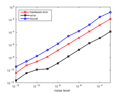
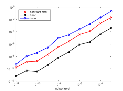
Test 4: noise level. In this test, we fix the number of matrices $m=16$. For different partitions $\tau_{n}=(3,3,3)$ and $\tau_{n}=(1,2,3)$, in Figure 1, we plot $\varepsilon_{\operatorname{bker}}$ (backward error), error and $\varepsilon_{\operatorname{ub}}$ (bound) versus different noise levels. We can see from Figure 1 that as $\xi$ increases, $\varepsilon_{\operatorname{bker}}$, error and $\varepsilon_{\operatorname{ub}}$ all increase almost linearly. For all noise levels, $\varepsilon_{\operatorname{ub}}$ indeed provides a good upper bound on the error.

$\tau_{n}=(3,3,3)$                                  $\tau_{n}=(1,2,3)$

Figure 1: Backward error $\varepsilon_{\operatorname{bker}}$, error, and bound $\varepsilon_{\operatorname{ub}}$ vs. noise level

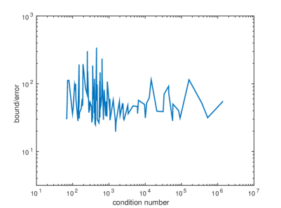
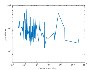
Test 5: condition number. In this test, we fix $m=16$, $\xi=10^{-12}$. For two different partitions $\tau_{n}=(3,3,3)$ and $\tau_{n}=(1,2,3)$, we ran the tests 100 times for each partition. In Figure 2, we plot the quotient $\varepsilon_{\operatorname{ub}}$/error versus the condition number $\operatorname{cond}(\mathcal{A})$. The smaller the quotient is, the sharper $\varepsilon_{\operatorname{ub}}$ estimates the error. We can see from Figure 2 that $\varepsilon_{\operatorname{ub}}$ provides a good upper bound on the error, even as the condition number becomes large.

$\tau_{n}=(3,3,3)$                                  $\tau_{n}=(1,2,3)$

Figure 2: Bound $\varepsilon_{\operatorname{ub}}$/error vs. condition number $\operatorname{cond}(\mathcal{A})$

6 Concluding Remarks

In this paper, we developed a perturbation theory for jbdp. An upper bound is obtained for the relative distance (1.5) between a block diagonalizer $W$ for the original jbdp of $\mathcal{A}$ that is block diagonalizable and an approximate diagonalizer $\widetilde{W}$ for its perturbed jbdp of $\widetilde{\mathcal{A}}$. The backward error and condition number are also derived and discussed for jbdp. Numerical tests validate the theoretical results.

The jbdp of interest in this paper is for block diagonalization via congruence transformations which are known to preserve symmetry. Yet our development so far does not assume that all $A_{i}$ are symmetric. What will happen to all the results if they are symmetric? It turns out that not much simplification in results and arguments can be gained but all the results remain valid after minor changes to the definitions of $G_{jk}$ in (2.7b): remove the second, fourth, $\ldots$, block rows as now all $A_{i}^{(jj)}$ are symmetric.

We have been limiting all the matrices to real ones, but this is not a limitation. In fact, if all matrices are complex, the change that needs to be made is simply to replace all transposes $\scriptstyle\operatorname{T}$ by complex conjugate transposes $\scriptstyle\operatorname{H}$, but for simplicity we still would like to keep all $\gamma_{i}$, the diagonal entries of $\Gamma$ real, so that we don’t have to change the definition of the gap $g$ in (3.5).

Conceivably, we might use similarity transformation for block diagonalization, i.e., instead of (1.3), we may seek a nonsingular matrix $W\in\mathbb{R}^{n\times n}$ such that all $W^{-1}A_{i}W$ are $\tau_{n}$-block diagonal. A similar development that are very much parallel to those in [3] and in this paper can be worked out. A major change will be to redefine the subspace $\mathscr{N}(\mathcal{A})$ in (2.2) as

$$\mathscr{N}(\mathcal{A}):=\big{\{}Z\in\mathbb{R}^{n\times n}\;:\;A_{i}Z-ZA_{i}=0\,\,\mbox{for $1\leq i\leq m$}\big{\}}.$$

We omit the detail.

References

• [1] B. Afsari. Sensitivity analysis for the problem of matrix joint diagonalization. SIAM J. Matrix Anal. Appl., 30(3):1148–1171, 2008.
• [2] Y. Bai, E. de Klerk, D. Pasechnik, and R. Sotirov. Exploiting group symmetry in truss topology optimization. Optim. Engrg., 10(3):331–349, 2009.
• [3] Y. Cai and C. Liu. An algebraic approach to nonorthogonal general joint block diagonalization. SIAM J. Matrix Anal. Appl., 38(1):50–71, 2017.
• [4] J.-F. Cardoso. Multidimensional independent component analysis. In Acoustics, Speech and Signal Processing, 1998. Proceedings of the 1998 IEEE International Conference on, volume 4, pages 1941–1944. IEEE, Washinton, DC, 1998.
• [5] G. Chabriel, M. Kleinsteuber, E. Moreau, H. Shen, P. Tichavsky, and A. Yeredor. Joint matrices decompositions and blind source separation: A survey of methods, identification, and applications. IEEE Signal Process. Mag., 31(3):34–43, 2014.
• [6] E. De Klerk, D. V. Pasechnik, and A. Schrijver. Reduction of symmetric semidefinite programs using the regular $\ast$-representation. Math. Program., 109(2-3):613–624, 2007.
• [7] E. De Klerk and R. Sotirov. Exploiting group symmetry in semidefinite programming relaxations of the quadratic assignment problem. Math. Program., 122(2):225–246, 2010.
• [8] L. De Lathauwer. Decompositions of a higher-order tensor in block terms-part I: Lemmas for partitioned matrices. SIAM J. Matrix Anal. Appl., 30(3):1022–1032, 2008.
• [9] L. De Lathauwer. Decompositions of a higher-order tensor in block terms-part II: Definitions and uniqueness. SIAM J. Matrix Anal. Appl., 30(3):1033–1066, 2008.
• [10] L. De Lathauwer. A survey of tensor methods. In 2009 IEEE International Symposium on Circuits and Systems, pages 2773–2776. IEEE, 2009.
• [11] L. De Lathauwer, B. De Moor, and J. Vandewalle. Fetal electrocardiogram extraction by blind source subspace separation. IEEE Trans. Biomedical Engrg., 47(5):567–572, 2000.
• [12] L. De Lathauwer and D. Nion. Decompositions of a higher-order tensor in block terms-part III: Alternating least squares algorithms. SIAM J. Matrix Anal. Appl., 30(3):1067–1083, 2008.
• [13] J. W. Demmel. Applied Numerical Linear Algebra. SIAM, Philadelphia, PA, 1997.
• [14] I. Domanov and L. De Lathauwer. On the uniqueness of the canonical polyadic decomposition of third-order tensors–part I: Basic results and uniqueness of one factor matrix. SIAM J. Matrix Anal. Appl., 34(3):855–875, 2013.
• [15] I. Domanov and L. De Lathauwer. On the uniqueness of the canonical polyadic decomposition of third-order tensors–part II: Uniqueness of the overall decomposition. SIAM J. Matrix Anal. Appl., 34(3):876–903, 2013.
• [16] K. Gatermann and P. A. Parrilo. Symmetry groups, semidefinite programs, and sums of squares. J. Pure Appl. Algebra, 192(1):95–128, 2004.
• [17] W. Kahan. Spectra of nearly hermitian matrices. Proc. Amer. Math. Soc., 48(1):11–17, 1975.
• [18] J. B. Kruskal. Three-way arrays: rank and uniqueness of trilinear decompositions, with application to arithmetic complexity and statistics. Linear Algebra Appl., 18(2):95–138, 1977.
• [19] R.-C. Li. Matrix perturbation theory. In L. Hogben, R. Brualdi, and G. W. Stewart, editors, Handbook of Linear Algebra, chapter 21. CRC Press, Boca Raton, FL, 2nd edition, 2014.
• [20] D. Nion. A tensor framework for nonunitary joint block diagonalization. IEEE Trans. Signal Process., 59(10):4585–4594, 2011.
• [21] B. Póczos and A. Lőrincz. Independent subspace analysis using k-nearest neighborhood distances. In Artificial Neural Networks: Formal Models and Their Applications-ICANN 2005, pages 163–168. Springer, 2005.
• [22] F. G. Russo. On an argument of j.-f. cardoso dealing with perturbations of joint diagonalizers. 2011. Available at arXiv:1103.3670.
• [23] D. C. Shi, Y. F. Cai, and S. F. Xu. Some perturbation results for a normalized non-orthogonal joint diagonalization problem. Linear Algebra Appl., 484:457–476, 2015.
• [24] M. Sørensen and L. De Lathauwer. Coupled canonical polyadic decompositions and (coupled) decompositions in multilinear rank-(Lr,n,Lr,n,1) terms–part I: Uniqueness. SIAM J. Matrix Anal. Appl., 36(2):496–522, 2015.
• [25] M. Sørensen and L. De Lathauwer. New uniqueness conditions for the canonical polyadic decomposition of third-order tensors. SIAM J. Matrix Anal. Appl., 36(4):1381–1403, 2015.
• [26] A. Stegeman. On uniqueness of the canonical tensor decomposition with some form of symmetry. SIAM J. Matrix Anal. Appl., 32(2):561–583, 2011.
• [27] G. W. Stewart and J.-G. Sun. Matrix Perturbation Theory. Academic Press, Boston, 1990.
• [28] J. G. Sun. On the variation of the spectrum of a normal matrix. Linear Algebra Appl., 246:215 – 223, 1996.
• [29] F. J. Theis. Blind signal separation into groups of dependent signals using joint block diagonalization. In Circuits and Systems, 2005. ISCAS 2005. IEEE International Symposium on, pages 5878–5881. IEEE, 2005.
• [30] F. J. Theis. Towards a general independent subspace analysis. In Advances in Neural Information Processing Systems, pages 1361–1368, MIT Press, Cambridge, MA, 2006.
• [31] P. Tichavsky, A. H. Phan, and A. Cichocki. Non-orthogonal tensor diagonalization. 2014. Available at arXiv:1402.1673v3.
• [32] C. F. Van Loan and G. H. Golub. Matrix computations. Johns Hopkins University Press, Baltimore, MD, 4th edition, 2012.
• [33] N. Vannieuwenhoven. A condition number for the tensor rank decomposition. 2016. Available at arXiv:1604.00052.
• [34] N. Vervliet, O. Debals, L. Sorber, M. Van Barel, and L. De Lathauwer. Tensorlab 3.0, March 2016. Available at www.tensorlab.net.