Abstract

Detecting weak seismic events from noisy sensors is a difficult perceptual task. We formulate this task as Bayesian inference and propose a generative model of seismic events and signals across a network of spatially distributed stations. Our system, SIGVISA, is the first to directly model seismic waveforms, allowing it to incorporate a rich representation of the physics underlying the signal generation process. We use Gaussian processes over wavelet parameters to predict detailed waveform fluctuations based on historical events, while degrading smoothly to simple parametric envelopes in regions with no historical seismicity. Evaluating on data from the western US, we recover three times as many events as previous work, and reduce mean location errors by a factor of four while greatly increasing sensitivity to low-magnitude events.

1 Introduction

The world contains structure: objects with dynamics governed by physical law. Intelligent systems must infer this structure from noisy, jumbled, and lossy sensory data. Bayesian statistics provides a natural framework for designing such systems: given a prior distribution $p(z)$ on underlying descriptions of the world, and a forward model $p(x|z)$ describing the process by which observations are generated, mathematical probability defines the posterior $p(z|x)\propto p(z)p(x|z)$ over worlds given observed data. Bayesian generative models have recently shown exciting results in applications ranging from visual scene understanding (Kulkarni et al., 2015; Eslami et al., 2016) to inferring celestial bodies (Regier et al., 2015).

In this paper we apply the Bayesian framework directly to a challenging perceptual task: monitoring seismic events from a network of spatially distributed sensors. This task is motivated by the Comprehensive Test Ban Treaty (CTBT), which bans testing of nuclear weapons and provides for the establishment of an International Monitoring System (IMS) to detect nuclear explosions, primarily from the seismic signals that they generate. The inadequacy of existing monitoring systems was cited as a factor in the US Senate’s 1999 decision not to ratify the treaty.

Our system, SIGVISA (Signal-based Vertically Integrated Seismic Analysis), consists of a generative probability model of seismic events and signals, with interpretable latent variables for physically meaningful quantities such as the arrival times and amplitudes of seismic phases. A previous system, NETVISA (Arora et al., 2013), assumed that signals had been preprocessed into discrete detections; we extend this by directly modeling seismic waveforms. This allows our model to capture rich physical structure such as path-dependent modulation as well as predictable travel times and attenuations. Inference in our model recovers a posterior over event histories directly from waveform traces, combining top-down with bottom-up processing to produce a joint interpretation of all observed data. In particular, Bayesian inference provides a principled approach to combining evidence from phase travel times and waveform correlations, a previously unsolved problem in seismology.

A full description of our system is given by Moore (2016); this paper describes the core model and key points of training and inference algorithms. Evaluating against existing systems for seismic monitoring, we show that SIGVISA significantly increases event recall at the same precision, detecting many additional low-magnitude events while reducing mean location error by a factor of four. Initial results indicate we also perform as well or better than existing systems at detecting events with no nearby historical seismicity.

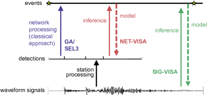
Figure 1: High level structure of traditional detection-based monitoring (GA), Bayesian monitoring (NETVISA), and signal-based Bayesian monitoring (SIGVISA, this work). Compared to detection-based approaches, inference in a signal-based model incorporates rich information from seismic waveforms.

2 Seismology background

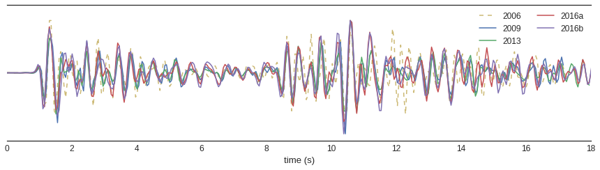
Figure 2: Aligned seismic waveforms (station MDJ, amplitude-normalized and filtered to 0.8-4.5Hz) from five events at the North Korean nuclear test site, showing strong inter-event correlation. By modeling this repeated structure, new events at this site can be detected even if only observed by a single station.

We model seismic events as point sources, localized in space and time, that release energy in the form of seismic waves. These include compression and shear (P and S) waves that travel through the solid earth, as well as surface waves such as Love and Rayleigh waves. Waves are further categorized into phases according to the path traversed from the source to a detecting station; for example, we distinguish P waves propagating directly upwards to the surface (Pg phases) from the same waves following a path guided along the crust-mantle boundary (Pn phases), among other options.

Given an event’s location, it is possible to predict arrival times for each phase by considering the length and characteristics of the event–station path. Seismologists have developed a number of travel time models, ranging from simple models that condition only on event depth and event-station distance (Kennett and Engdahl, 1991), to more sophisticated models that use an event’s specific location to provide more accurate predictions incorporating the local velocity structure (Simmons et al., 2012). Inverting the predictions of a travel-time model allows events to be located by triangulation given a set of arrival times.

Seismic stations record continuous ground motion along one or more axes, including background noise from natural and human sources, as well as the signals generated by arriving seismic phases. The detailed fluctuations in these signals are a function of the source as well as a path-dependent transfer function, in which seismic energy is modulated and distorted by the geological characteristics of the event–station path. Since geology does not change much over time, events with similar locations and depths tend to generate highly correlated waveforms (Figure 2); the lengthscale at which such correlations are observed depends on the local geology and may range from hundreds of meters up to tens of kilometers.

2.1 Seismic monitoring systems

Traditional architectures for seismic monitoring operate via bottom-up processing (Figure 1). The waveform at each station is thresholded to produce a feature representation consisting of discrete “detections” of possible phase arrivals. Network processing attempts to associate detections from all stations into a coherent set of events. Potential complications include false detections caused by noise, and missed detections from arrivals for which the station processing failed to trigger. In addition, the limited information (estimated arrival time, amplitude, and azimuth) in a single detection means that an event typically requires detections from at least three stations to be formed.

The NETVISA system (Arora et al., 2010, 2013) replaces heuristic network processing with Bayesian inference in a principled model of seismic events and detections, including probabilities of false and missing detections. Maximizing posterior probability in this model via hill-climbing search yields an event bulletin that incorporates all available data accounting for uncertainty. Because NETVISA separates inference from the construction of an explicit domain model, domain experts can improve system performance simply by refining the model. Compared to the IMS’s previous network processing system (Global Association, or GA), NETVISA provides significant improvements in location accuracy and a 60% reduction in missed events; as of this writing, it has been proposed by the UN as the new production monitoring system for the CTBT.

Recently, new monitoring approaches have been proposed using the principle of waveform matching, which exploits correlations between signals from nearby events to detect and locate new events by matching incoming signals against a library of historical signals. These promise the ability to detect events up to an order of magnitude below the threshold of a detection-based system (Gibbons and Ringdal, 2006; Schaff and Waldhauser, 2010), and to locate such events even from a single station (Schaff et al., 2012). However, adoption has been hampered by the inability to detect events in locations with no historical seismicity, a crucial requirement for nuclear monitoring. In addition, it has not been clear how to quantify the reliability of events detected by waveform correlation, how to reconcile correlation evidence from multiple stations, or how to combine correlation and detection-based methods in a principled way. Our work resolves these questions by showing that both triangulation and waveform matching behaviors emerge naturally during inference in a unified generative model of seismic signals.

3 Modeling seismic waveforms

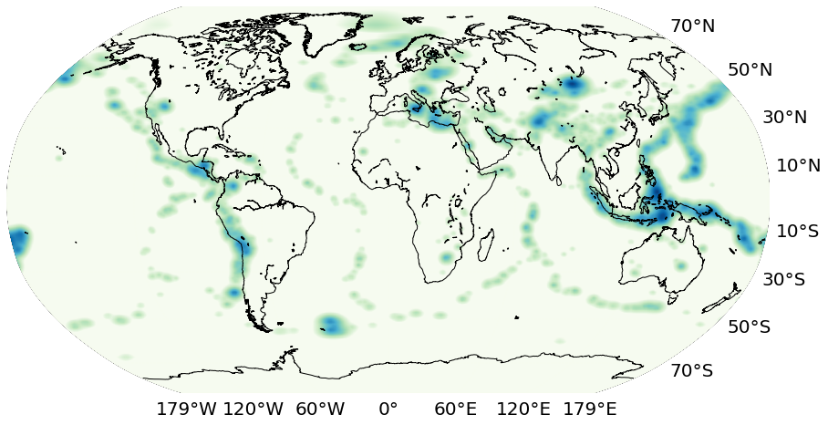
Figure 3: Global prior on seismic event locations.

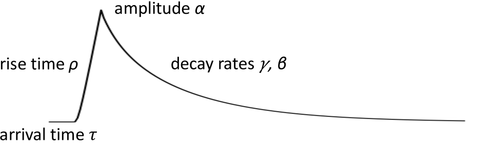
(a) Parametric form $g(t;\mathbf{\theta})$ modeling the signal envelope of a single arriving phase. (eq. 2)

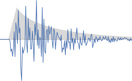
(b) Signal for an arriving phase, generated by multiplying the parametric envelope $g$ (shaded) by a zero-mean modulation signal $m(t;\mathbf{w})$. (eq. 3)

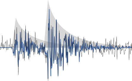
(c) The final generated signal $\mathbf{s}_{j}$ sums the contributions of all arriving phases with an autoregressive background noise process. (eqs. 4 and 5)

Figure 4: Steps of the SIGVISA forward model.

SIGVISA (our current work) extends NETVISA by incorporating waveforms directly in the generative model, eliminating the need for bottom-up detection processing. Our model describes a joint distribution $p(\mathbf{E},\mathbf{S})=p(\mathbf{S}|\mathbf{E})p(\mathbf{E})$ on $n_{E}$ seismic events $\mathbf{E}$ and signals $\mathbf{S}$ observed across $n_{S}$ stations. We model event occurrence as a time-homogenous Poisson process,

$$p(n_{E})=\text{Poisson}(\lambda T),\;p(\mathbf{E})=p(n_{E})n_{E}!\prod_{i=1}^{n_{E}}p(\mathbf{e}_{i}),$$

so that the number of events generated during a time period of length $T$ is itself random, and each event is sampled independently from a prior $p(\mathbf{e}_{i})$ over surface location, depth, origin time, and magnitude. The homogeneous process implies a uniform prior on origin times, with a labeling symmetry that we correct by multiplying by the permutation count $n_{E}!$. Location and depth priors, along with the event rate $\lambda$, are estimated from historical seismicity as described by Arora et al. (2013). The location prior is a mixture of a kernel density estimate of historical events, and a uniform component to allow explosions and other events in locations with no previous seismicity (Figure 3).

We assume that signals at different stations are conditionally independent, given events, and introduce auxiliary variables $\mathbf{\theta}$ and $\mathbf{w}$ governing signal generation at each station, so that the forward model has the form

$$p(\mathbf{S}|\mathbf{E})=\prod_{j=1}^{n_{S}}\left(\iint p(\mathbf{s}_{j}|\mathbf{\theta}_{j},\mathbf{w}_{j})p(\mathbf{\theta}_{j}|\mathbf{E})p(\mathbf{w}_{j}|\mathbf{E})d\mathbf{w}_{j}d\mathbf{\theta}_{j}\right).$$ (1)

The parameters $\mathbf{\theta}$ describe an envelope shape for each arriving phase, and $\mathbf{w}$ describes repeatable modulation processes that multiply these envelopes to generate observed waveforms (Figure 4). In particular, we decompose these into independent (conditioned on event locations) components $\mathbf{\theta}_{i,j,k}$ and $\mathbf{w}_{i,j,k}$ describing the arrival of phase $k$ of event $i$ at station $j$.

The envelope of each phase is modeled by a linear onset followed by a poly-exponential decay (Figure 4(a)),

$$g(t;\theta_{i,j,k})=\left\{\begin{array}[]{ll}0&\text{ if }t\leq\tau\\ \alpha(t-\tau)/\rho&\text{ if }\tau<t\leq\tau+\rho\\ \alpha(t-\tau+1)^{-\gamma}e^{-\beta(t-\tau)}&\text{ otherwise}\\ \end{array}\right.$$ (2)

with parameters $\theta_{i,j,k}=(\tau,\rho,\alpha,\gamma,\beta)_{i,j,k}$ consisting of an arrival time $\tau$, rise time $\rho$, amplitude $\alpha$, and decay rates $\gamma$ and $\beta$ governing respectively the envelope peak and its coda, or long-run decay. This decay form is inspired by previous work modeling seismic coda (Mayeda et al., 2003), while the linear onset follows that used by Cua (2005) for seismic early warning.

To produce a signal, the envelope is multiplied by a modulation process $m$ (Figure 4(b)), parameterized by wavelet coefficients $\mathbf{w}_{i,j,k}$ so that

$$m(t;\mathbf{w}_{i,j,k})=\left\{\begin{array}[]{ll}(\mathbf{D}\mathbf{w}_{i,j,k})(t)&\text{if }0\leq t<20s\\ \mathbf{\varepsilon}(t)&\text{otherwise}\end{array}\right.$$ (3)

where $\mathbf{D}$ is a discrete wavelet transform matrix, and $\mathbf{\varepsilon}(t)\sim\mathcal{N}(0,1)$ is a Gaussian white noise process. We explicitly represent coefficients describing the first 20 seconds of each arrival, and model the modulation as random after that point. We use an order-4 Daubechies wavelet basis (Daubechies, 1992), so that for 10Hz signals each $\mathbf{w}_{i,j,k}$ is a vector of 220 coefficients. As described below, we model $\mathbf{w}$ jointly across events using a Gaussian process, so that our modulation processes are repeatable: events in nearby locations will generate correlated signals (Figure 5).

Summing the signals from all arriving phases yields the predicted signal $\mathbf{\bar{s}}_{j}$,

$$\bar{s}_{j}(t)=\sum_{i,k}g(t;\mathbf{\theta}_{i,j,k})\cdot m(t-\tau_{i,j,k};\mathbf{w}_{i,j,k});$$ (4)

and we generate the observed signal $\mathbf{s_{j}}$ (Figure 4(c)) by adding an order-$R$ autoregressive noise process,

$$p(\mathbf{s}_{j}|\mathbf{\theta}_{j},\mathbf{w}_{j}) =p_{AR}(\mathbf{s}_{j}-\mathbf{\bar{s}}_{j}-\mu_{j};\sigma^{2}_{j},\mathbf{\phi}_{j})$$ (5)

$$p_{AR}(\mathbf{z};\sigma^{2},\mathbf{\phi}) =\prod_{t=1}^{T}\mathcal{N}\left(z(t);\sum_{r=1}^{R}\mathbf{\phi}_{r}z(t-r),\sigma^{2}\right).$$

We adapt the noise process online during inference, following station-specific priors on the mean $p(\mu_{j})$, variance $p(\sigma^{2}_{j})$, and autoregressive coefficients $p(\mathbf{\phi}_{j})$.

3.1 Repeatable signal descriptions

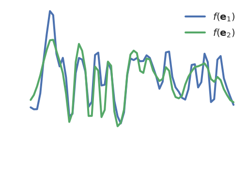
(a) Co-located sources.

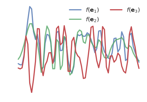
(b) Adding a distant source.

Figure 5: Samples from a GP prior on db4 wavelets.

For each station $j$ and phase $k$, we model the signal descriptions $p(\mathbf{\theta}_{j,k}|\mathbf{E})$ and $p(\mathbf{w}_{j,k}|\mathbf{E})$ jointly across events as Gaussian process transformations of the event space $\mathbf{E}$ (Rasmussen and Williams, 2006), so that events in nearby locations will tend to generate similar envelope shapes and correlated modulation signals, allowing our system to detect and locate repeated events even from a weak signal recorded at a single station. Since the events are unobserved, this is effectively a GP latent variable model (Lawrence, 2004), with the twist that in our model the outputs $\mathbf{\theta},\mathbf{w}$ are themselves latent variables, observed only indirectly through the signal model $p(\mathbf{S}|\mathbf{\theta},\mathbf{w})$.

We borrow models from geophysics to predict the arrival time and amplitude of each phase: given the origin time, depth, and event-station distance, the IASPEI-91 (Kennett and Engdahl, 1991) travel-time model predicts an arrival time $\bar{\tau}$, and the Brune source model (Brune, 1970) predicts a source (log) amplitude $\log\bar{\alpha}$ as a function of event magnitude. We then use GPs to model deviations from these physics-based predictions; that is, we take $\bar{\tau}$ and $\log\bar{\alpha}$ as the mean functions for GPs modeling $\tau$ and $\log\alpha$ respectively. The remaining shape parameters $\rho,\gamma,\beta$ (in log space) and the 220 wavelet coefficients in $\mathbf{w}_{i,j,k}$ are each modeled by independent zero-mean GPs.

Parameter	Features $\phi(\mathbf{e})$
Arrival time ($\tau$)	n/a
Amplitude (log $\alpha$)	$\left(1,\Delta,\sin(\frac{\Delta}{15000}),\cos(\frac{\Delta}{15000})\right)$
Onset (log $\rho$)	(1, mb)
Peak decay (log $\gamma$)	(1, mb, $\Delta$)
Coda decay (log $\beta$)	(1, mb, $\Delta$)
Wavelet coefs ($w$)	n/a

Table 1: Feature representations in terms of magnitude mb and event–station distance $\Delta$ (km).

All of our GPs share a common covariance form,

$$k(\mathbf{e},\mathbf{e}^{\prime})=\phi(\mathbf{e})^{T}\mathbf{B}\phi(\mathbf{e}^{\prime})+\sigma^{2}_{f}k_{\text{Mat\'{e}rn}}(d_{\ell}(\mathbf{e},\mathbf{e}^{\prime}))+\sigma^{2}_{n}\delta,$$

where the first term models an unknown function that is linear in some feature representation $\phi$, chosen separately for each parameter (Table 1). This represents general regularities such as distance decay that we expect to hold even in regions with no observed training data. For efficiency and to avoid degenerate covariances we represent this component in weight space (Rasmussen and Williams, 2006, section 2.7); at test time we choose $\mathbf{B}$ to be the posterior covariance given training data. The second term models an unknown differentiable function using a stationary Matérn ($\nu=3/2$) kernel (Rasmussen and Williams, 2006, Chapter 4), with great-circle distance metric controlled by lengthscale hyperparameters $\ell$; this allows our model to represent detailed local seismic structure. We also include iid noise $\sigma^{2}_{n}\delta$ to encode unmodeled variation between events in the same location.

To enable efficient training and test-time GP predictions, we partition the training data into spatially local regions using $k$-means clustering, and factor the nonparametric (Matérn) component into independent regional models. This allows predictions in each region to be made efficiently using only a small number of nearby events, avoiding a naïve $O(n^{2})$ dependence on the entire training set. Each region is given separate hyperparameters, allowing our models to adapt to spatially varying seismicity.

3.2 Collapsed signal model

The explicit model described thus far exhibits tight coupling between envelope parameters and modulation coefficients; a small shift in a phase’s arrival time may significantly change the wavelets needed to explain an observed signal, causing inference moves that do not account for this joint structure to fail. Fortunately, it is possible to exactly marginalize out the coefficients $\mathbf{w}$ so that they do not need to be represented in inference. This follows from the linear Gaussian structure of our signal model: GPs induce a Gaussian distribution on wavelet coefficients, which are observed under linear projection (a wavelet transform followed by envelope scaling) with autoregressive background noise. Thus, the collapsed distribution $p(\mathbf{s}_{j}|\mathbf{\theta}_{j},\mathbf{E})=\int p(\mathbf{s}_{j}|\mathbf{\theta}_{j},\mathbf{w}_{j})p(\mathbf{w}_{j}|\mathbf{E})d\mathbf{w}_{j}$ is multivariate Gaussian, and in principle can be evaluated directly.

Doing this efficiently in practice requires exploiting graphical model structure. Specifically, we formulate the signal model at each station as a linear Gaussian state space model, with a state vector that tracks the AR noise process as well as the set of wavelet coefficients that actively contribute to the signal. Due to the recursive structure of wavelet bases, the number of such coefficients is only logarithmic at each timestep. We exploit this structure, the same used by fast wavelet transforms, to efficiently compute coefficient posteriors and marginal likelihoods by Kalman filtering (Grewal and Andrews, 2014).

We assume for efficiency that test-time signals from different events are independent given the training data. During training, however, it is necessary to compute the joint density of signals involving multiple events so that we can find correct alignments. This requires us to pass messages $f_{j}(\mathbf{w}_{j})=p(\mathbf{s}_{j}|\mathbf{w}_{j},\mathbf{\theta}_{j})$ from each signal upwards to the GP prior (Koller and Friedman, 2009). We compute a diagonal approximation

$$\tilde{f}_{j}(\mathbf{w}_{j})=\frac{1}{Z_{j}}\prod_{c=1}^{220}\mathcal{N}(\mathbf{w}_{j,c};\tilde{\nu}_{j,c},\tilde{\xi}_{j,c})$$

by dividing the Kalman filtering posterior on wavelet coefficients by the (diagonal Gaussian) prior. The product of these messages with the GP priors $p(\mathbf{w}_{c}|\mathbf{E})\sim\mathcal{N}(\mathbf{\mu}_{c}(\mathbf{E}),\mathbf{K}_{c}(\mathbf{E}))$, integrated over coefficients $\mathbf{w}$, gives an approximate joint density

$$p(\mathbf{S}|\mathbf{\theta},\mathbf{E})\approx\left(\prod_{j=1}^{N}\frac{1}{Z_{j}}\right)\prod_{c}\mathcal{N}\left(\bar{\nu}_{c};\mathbf{\mu}_{c}(\mathbf{E}),\mathbf{K}_{c}(\mathbf{E})+\mathbf{\tilde{\xi}}_{c}\right),$$ (6)

in which the wavelet GPs are evaluated at the values of (and with added variance given by) the approximate messages from observed signals. We target this approximate joint density during training, and condition our test-time models on the upwards messages generated by training signals.

4 Training

We train using a bulletin of historical event locations which we take as ground truth (relaxing this assumption to incorporate noisy training locations, or even fully unsupervised training, is important future work). Given observed events, we use training signals to estimate the GP models—hyperparameters as well as the upwards messages from training signals—along with priors $p(\mu_{j})$, $p(\sigma^{2}_{j})$, and $p(\mathbf{\phi}_{j})$ on background noise processes at each station. We use the EM algorithm (Dempster et al., 1977) to search for maximum likelihood parameters integrating over the unobserved noise processes and envelope shapes.

The E step runs MCMC inference (Section 5) to sample from the posterior over the latent variables $\mathbf{\theta},\mathbf{\mu},\mathbf{\sigma}^{2},\mathbf{\phi}$ under the collapsed objective described above. We approximate the sampled posterior on $\mathbf{\theta}$ by univariate Gaussians to compute approximate upwards messages. These are used in the M step to fit GP hyperparameters via gradient-based optimization of the marginal likelihood (6). The priors on background noise means $p(\mu_{j})$ and coefficients $p(\mathbf{\phi}_{j})$ are fit as Gaussian and multivariate Gaussian respectively. For the noise variance $\sigma^{2}_{j}$ at each station, we fit log-normal, inverse Gamma, and truncated Gaussian priors and select the most likely; this adapts for different noise distributions between stations.

5 Inference

We perform inference using reversible jump MCMC (Hastie and Green, 2012) applied to the collapsed model. Our algorithm consists of a cyclic sweep of single-site, random-walk Metropolis-Hastings moves over all currently instantiated envelope parameters $\mathbf{\theta}$, autoregressive noise parameters $\mu,\sigma^{2},\phi$ at each station, and event descriptions $(\mathbf{e}_{i})_{i=1}^{n_{E}}$ including surface location, depth, time, and magnitude. We also include custom moves that propose swapping the associations of consecutive arrivals, aligning observed signals with GP predicted signals, and shifting envelope peak times to match those of the observed signal.

To improve event mixing, we augment our model to include unassociated arrivals: phase arrivals not generated by any particular event, with envelope parameters and modulation from a fixed Gaussian prior. Unassociated arrivals are useful in allowing events to be built and destroyed piecewise, so that we are not required to perfectly propose an event and all of its phases in a single shot. They can also be viewed as small events whose locations have been integrated out. Our birth proposal generates unassociated arrivals with probability proportional to the signal envelope, so that periods of high signal energy are quickly explained by unassociated arrivals which may then be associated into larger events.

Event birth moves are constructed using two complementary proposals. The first is based on a Hough transform of unassociated arrivals; it grids the 5D event space (longitude, latitude, depth, time, magnitude) and scores each bin using the log likelihood of arrivals greedily associated with an event in that bin. The second proposal is a mixture of Gaussians centered at the training events, with weights determined by waveform correlations against test signals. This allows us to recover weak events that correlate with training signals, while the Hough proposal can construct events in regions with no previous seismicity.

In proposing a new event we must also propose envelope parameters for all of its phases. Each phase may associate a currently unassociated arrival; where there are no plausible arrivals to associate we parent-sample envelope parameters given the proposed event, then run auxiliary Metropolis-Hastings steps (Storvik, 2011) to adapt the envelopes to observed signals. The proposed event, associations, and envelope parameters are jointly accepted or rejected by a final MH step. Event death moves similarly involve jointly proposing an event to kill along with a set of phase arrivals to delete (with the remainder preserved as unassociated).

By chaining birth and death moves we also construct mode-jumping moves that repropose an existing event, along with split and merge moves that replace two existing events with a single one, and vice versa. Moore (2016) describes our inference moves in more detail.

6 Evaluation

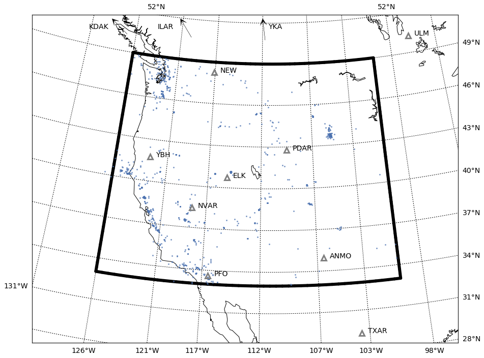
Figure 6: Training events (blue dots) from the western US dataset, with region of interest outlined. Triangles indicate IMS stations.

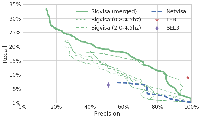
Figure 7: Precision-recall performance over the two-week test period, relative to the reference bulletin.

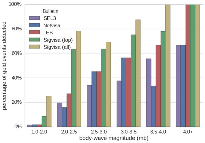
Figure 8: Event recall by magnitude range. The SIGVISA (top) bulletin is defined to match the precision of SEL3 (51%).

rb

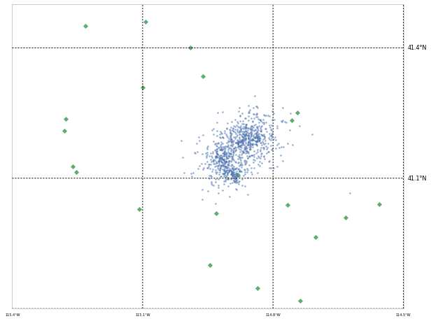
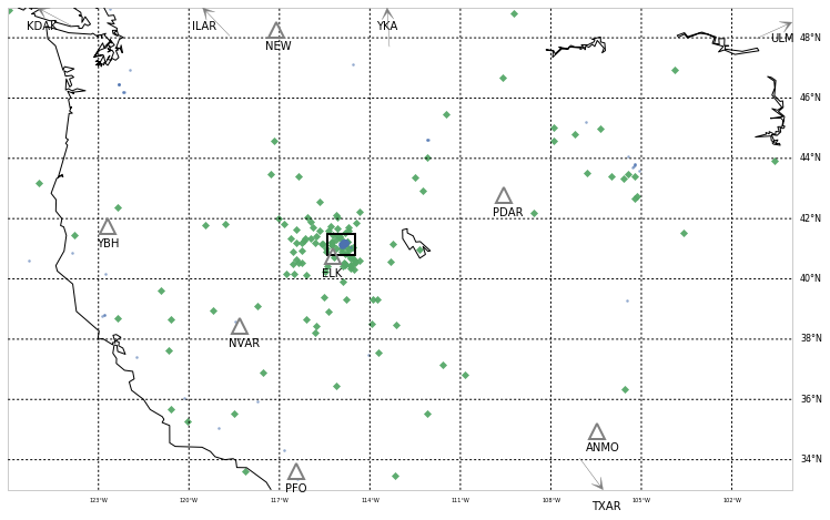
(a) NETVISA (139 events)

rb

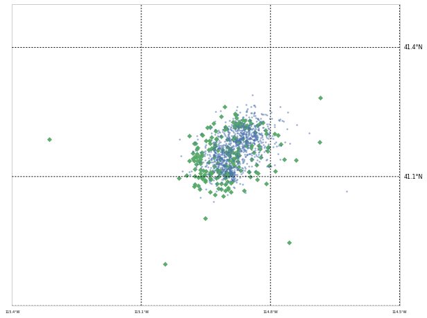
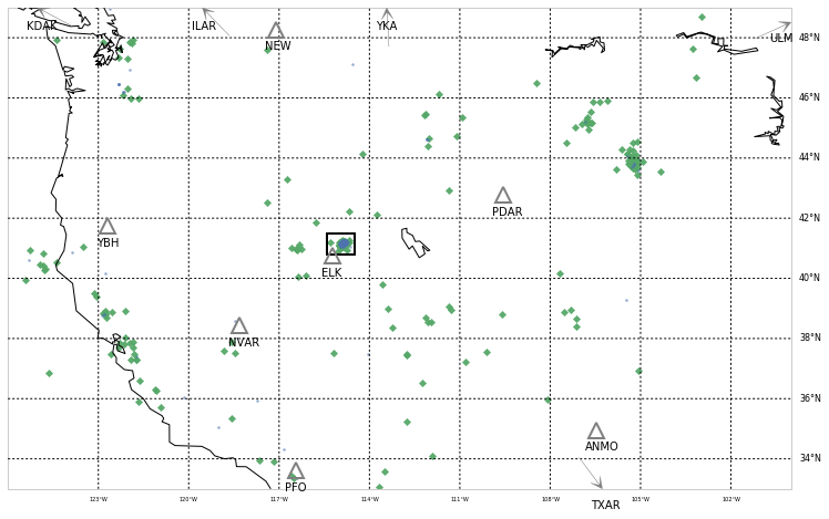
(b) SIGVISA top events (393 events)

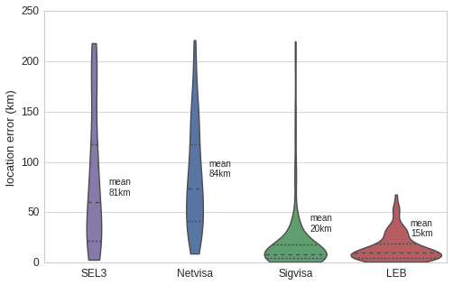
(c) Distribution of location errors.

Figure 9: Inferred events (green), with inset close-up of Wells aftershocks. Reference events are in blue.

We consider the task of monitoring seismic events in the western United States, which contains both significant natural seismicity and regular mining explosions. We focus in particular on the time period immediately following the magnitude 6.0 earthquake near Wells, NV, on February 21, 2008, which generated a large number of aftershocks. We train on one year of historical data (Figure 6), from January to December 2008; to enable SIGVISA to recognize aftershocks using waveform correlation, we also train on the first six hours following the Wells mainshock. The test period is two weeks long, beginning twelve hours after the Wells mainshock; the six hours immediately preceding were used as a validation set.

We compare SIGVISA’s performance to that of existing systems that also process data from the International Monitoring System. SEL3 is the final-stage automated bulletin from the CTBTO’s existing system (GA); it is reviewed by a team of human analysts to produce the Late Event Bulletin (LEB) reported to the member states. We also compare to the automated NETVISA bulletin(Arora et al., 2013), which implements detection-based Bayesian monitoring.

We construct a reference bulletin by combining events from regional networks aggregated by the National Earthquake Information Center (NEIC), and an analysis of aftershocks from the Wells earthquake based on data from the transportable US Array and temporary instruments deployed by the University of Nevada, Reno (UNR) (Smith et al., 2011). Because the reference bulletin has access to many sensors not included in the IMS, it is a plausible source of “ground truth” to evaluate the IMS-based systems.

We trained two sets of SIGVISA models, on broadband (0.8-4.5Hz) signals as well as a higher-frequency band (2.0-4.5Hz) intended to provide clearer evidence of regional events, using events observed from the reference bulletin. To produce a test bulletin, we ran three MCMC chains on broadband signals and two on high-frequency signals, and merged the results using a greedy heuristic that iteratively selects the highest-scoring event from any chain excluding duplicates. Each individual chain was parallelized by dividing the test period into 168 two-hour blocks and running independent inference on each block of signals. Overall SIGVISA inference used 840 cores for 48 hours.

We evaluate each system by computing a minimum weight maximum cardinality matching between the inferred and reference bulletins, in a bipartite graph with edges weighted by distance and restricted to events separated by at most $2^{\circ}$ in distance and 50s in time. Using this matching, we report precision (the percentage of inferred events that are real), recall (the percentage of real events detected by each system), and mean location error of matched events. For NETVISA and SIGVISA, which attach a confidence score to each event, we report a precision-recall curve parameterized by the confidence threshold (Figure 7).

Our results show that the merged SIGVISA bulletin dominates both NETVISA and SEL3. When operating at the same precision as SEL3 (51%), SIGVISA achieves recall three times higher than SEL3 (19.3% vs 6.4%), also eclipsing the 7.3% recall achieved by NETVISA at a slightly higher precision (54.7%). The human-reviewed LEB achieves near-perfect precision but only 9% recall, confirming that many events recovered by SIGVISA are not obvious to human analysts. The most sensitive SIGVISA bulletin recovers a full 33% of the reference events, at the cost of many more false events (14% precision).

Signal-based modeling particularly improves recall for low-magnitude events (Figure 8) for which bottom-up processing may not register detections. We also observe improved locations (Figure 9) for clusters such as the Wells aftershock sequence where observed waveforms can be matched against training data.

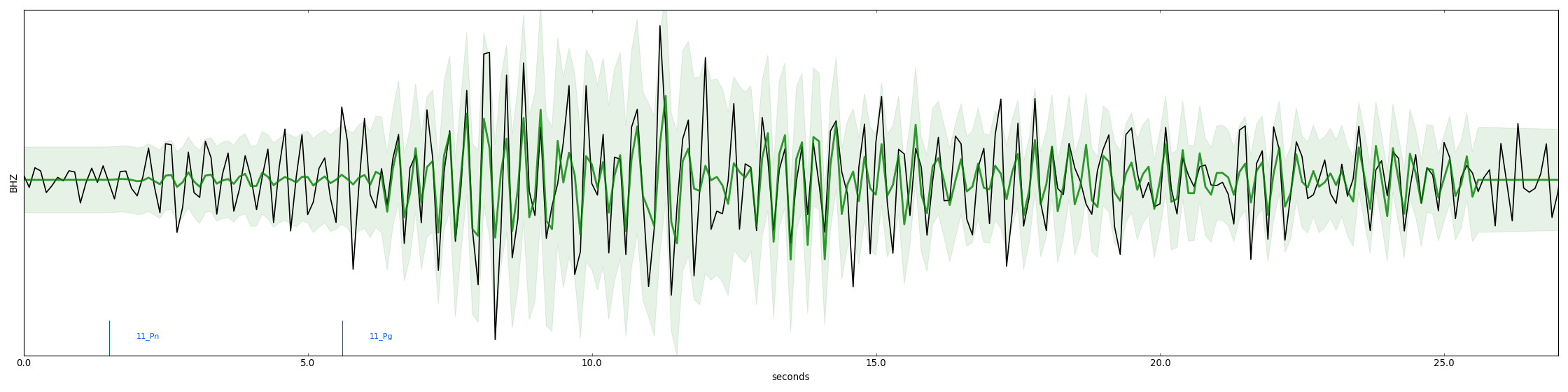
(a) Likely mining explosion at Black Thunder Mine. Location 105.21^∘ W, 43.75^∘ N, depth 1.9km, origin time 17:15:58 UTC, 2008-02-27, mb 2.6, recorded at PDAR (PD31).

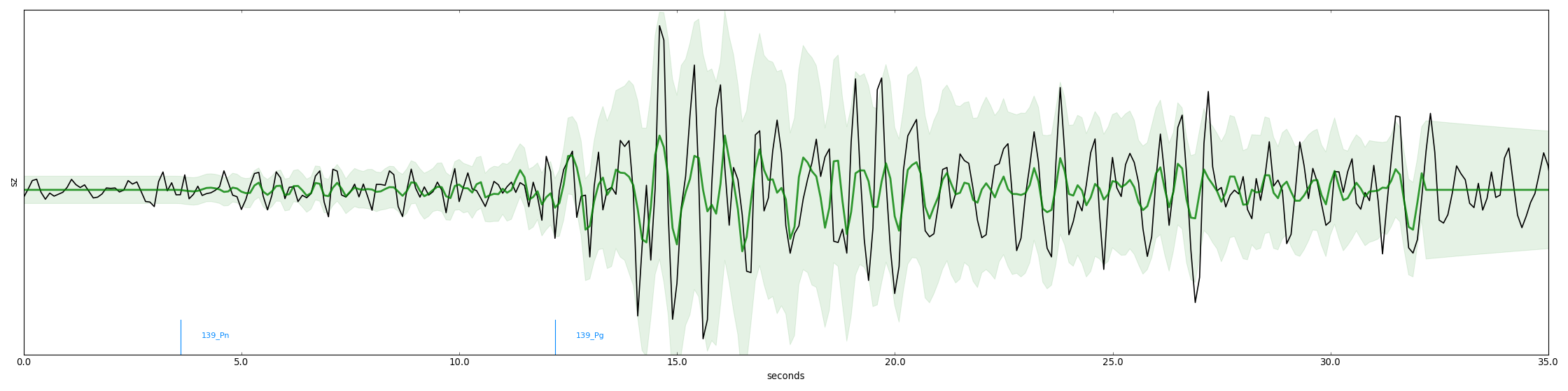
(b) Event near Cloverdale, CA along the Rodgers Creek fault. Location 122.79^∘ W, 38.80^∘ N, depth 1.6km, origin time 05:20:56 UTC, 2008-02-29, mb 2.6, recorded at NVAR (NV01).

Figure 10: Waveform evidence for two events detected by SIGVISA but not the reference bulletin. Green indicates the model predicted signal (shaded $\pm 2\sigma$); black is the observed signal (filtered 0.8-4.5Hz).

Interestingly, because we do not have access to absolute ground truth, some events labeled as false in our evaluation may actually be genuine events missed by the reference bulletin. Figure 10 shows two candidates for such events, with strong correspondence between the model-predicted and observed waveforms. The existence of such events provides reason to believe that SIGVISA’s true performance on this dataset is modestly higher than our evaluation suggests.

6.1 de novo events

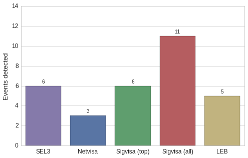
Figure 11: Recall for 24 de novo events between January and March 2008.

For nuclear monitoring it is particularly important to detect de novo events: those with no nearby historical seismicity. We define “nearby” as within 50km. Our two-week test period includes only three such events, so we broaden the scope to the three-month period of January through March 31, 2008, which includes 24 de novo events. We evaluated each system’s recall specifically on this set: of the 24 de novo reference events, how many were detected?

As shown in Figure 11, SIGVISA’s performance matches or exceeds the other systems. Operating at the same precision as SEL3, it detects the same number (6/24) of de novo events. This suggests that SIGVISA’s improved performance on repeated events—including almost all of the natural seismicity in the western US during our two-week test period—does not come at a cost for de novo events. To the contrary, the full high-sensitivity SIGVISA bulletin includes six genuine events missed by all other IMS-based systems.

7 Discussion

Our results demonstrate the promise of Bayesian inference on raw waveforms for monitoring seismic events. Applying MCMC inference to a generative probability model of repeatable seismic signals, we recover up to three times as many events as a detection-based baseline (SEL3) while operating at the same precision, and reduce mean location errors by a factor of four while greatly increasing sensitivity to low-magnitude events. Our system maintains effective performance even for events in regions with no historical seismicity in the training set.

A major advantage of the generative formulation is that the explicit model is interpretable by domain experts. We continue to engage with seismologists on potential model improvements, including tomographic travel-time models, directional information from seismic arrays and horizontal ground motion, and explicit modeling of earthquake versus explosion sources. Additional directions include more precise investigations of our model’s ability to quantify uncertainty and to estimate its own detection limits as a function of network coverage and historical seismicity. We also expect to continue scaling to global seismic data, exploiting parallelism and refining our inference moves and implementation. More generally, we hope that successful application of complex Bayesian models will inspire advances in probabilistic programming systems to make generative modeling accessible to a wider scientific audience.

Acknowledgements

We are very grateful to Steve Myers (LLNL) and Kevin Mayeda (Berkeley/AFTAC) for sharing their expertise on seismic modeling and monitoring and advising on the experimental setup. This work is supported by the Defense Threat Research Agency (DTRA) under grant #HDTRA-1111-0026, and experiments by an Azure for Research grant from Microsoft.

References

- Arora et al. (2013) Arora, N., Russell, S., and Sudderth, E. (2013). Net-visa: Network Processing Vertically Integrated Seismic Analysis. Bulletin of the Seismological Society of America, 103(2A):709–729.
- Arora et al. (2010) Arora, N., Russell, S. J., Kidwell, P., and Sudderth, E. B. (2010). Global seismic monitoring as probabilistic inference. In Advances in Neural Information Processing Systems, pages 73–81.
- Brune (1970) Brune, J. N. (1970). Tectonic stress and the spectra of seismic shear waves from earthquakes. Journal of Geophysical Research, 75(26):4997–5009.
- Cua (2005) Cua, G. B. (2005). Creating the Virtual Seismologist: Developments in Ground Motion Characterization and Seismic Early Warning. PhD thesis, California Institute of Technology.
- Daubechies (1992) Daubechies, I. (1992). Ten lectures on wavelets. In Regional conference Series in Applied Mathematics (SIAM), Philadelphia.
- Dempster et al. (1977) Dempster, A. P., Laird, N. M., and Rubin, D. B. (1977). Maximum likelihood from incomplete data via the EM algorithm. Journal of the royal statistical society. Series B (methodological), pages 1–38.
- Eslami et al. (2016) Eslami, S., Heess, N., Weber, T., Tassa, Y., Kavukcuoglu, K., and Hinton, G. E. (2016). Attend, infer, repeat: Fast scene understanding with generative models. arXiv preprint arXiv:1603.08575.
- Gibbons and Ringdal (2006) Gibbons, S. J. and Ringdal, F. (2006). The detection of low magnitude seismic events using array-based waveform correlation. Geophysical Journal International, 165(1):149–166.
- Grewal and Andrews (2014) Grewal, M. S. and Andrews, A. P. (2014). Kalman Filtering: Theory and Practice with MATLAB. John Wiley & Sons.
- Hastie and Green (2012) Hastie, D. I. and Green, P. J. (2012). Model choice using reversible jump Markov chain Monte Carlo. Statistica Neerlandica, 66(3):309–338.
- Kennett and Engdahl (1991) Kennett, B. and Engdahl, E. (1991). Traveltimes for global earthquake location and phase identification. Geophysical Journal International, 105(2):429–465.
- Koller and Friedman (2009) Koller, D. and Friedman, N. (2009). Probabilistic Graphical Models: Principles and Techniques. MIT Press.
- Kulkarni et al. (2015) Kulkarni, T. D., Kohli, P., Tenenbaum, J. B., and Mansinghka, V. (2015). Picture: A probabilistic programming language for scene perception. In Proceedings of the IEEE Conference on Computer Vision and Pattern Recognition (CVPR), pages 4390–4399.
- Lawrence (2004) Lawrence, N. D. (2004). Gaussian process latent variable models for visualisation of high dimensional data. In Advances in Neural Information Processing Systems (NIPS).
- Mayeda et al. (2003) Mayeda, K., Hofstetter, A., O’Boyle, J. L., and Walter, W. R. (2003). Stable and transportable regional magnitudes based on coda-derived moment-rate spectra. Bulletin of the Seismological Society of America, 93(1):224–239.
- Moore (2016) Moore, D. A. (2016). Signal-based Bayesian Seismic Monitoring. PhD thesis, University of California, Berkeley.
- Rasmussen and Williams (2006) Rasmussen, C. and Williams, C. (2006). Gaussian Processes for Machine Learning. MIT Press.
- Regier et al. (2015) Regier, J., Miller, A., McAuliffe, J., Adams, R., Hoffman, M., Lang, D., Schlegel, D., and Prabhat, M. (2015). Celeste: Variational inference for a generative model of astronomical images. In Proceedings of the 32nd International Conference on Machine Learning.
- Schaff et al. (2012) Schaff, D. P., Kim, W.-Y., and Richards, P. G. (2012). Seismological constraints on proposed low-yield nuclear testing in particular regions and time periods in the past. Science and Global Security, 20(2-3):155–171.
- Schaff and Waldhauser (2010) Schaff, D. P. and Waldhauser, F. (2010). One magnitude unit reduction in detection threshold by cross correlation applied to Parkfield (California) and China seismicity. Bulletin of the Seismological Society of America, 100(6):3224–3238.
- Simmons et al. (2012) Simmons, N. A., Myers, S. C., Johannesson, G., and Matzel, E. (2012). Llnl-g3dv3: Global P wave tomography model for improved regional and teleseismic travel time prediction. Journal of Geophysical Research: Solid Earth, 117(B10).
- Smith et al. (2011) Smith, K., Pechmann, J., Meremonte, M., and Pankow, K. (2011). Preliminary analysis of the mw 6.0 wells, nevada, earthquake sequence. Nevada Bureau of Mines and Geology Special Publication, 36:127–145.
- Storvik (2011) Storvik, G. (2011). On the flexibility of Metropolis–Hastings acceptance probabilities in auxiliary variable proposal generation. Scandinavian Journal of Statistics, 38(2):342–358.