Human Interaction with Recommendation Systems

Abstract

Many recommendation algorithms rely on user data to generate recommendations. However, these recommendations also affect the data obtained from future users. This work aims to understand the effects of this dynamic interaction. We propose a simple model where users with heterogeneous preferences arrive over time. Based on this model, we prove that naive estimators, i.e. those which ignore this feedback loop, are not consistent. We show that consistent estimators are efficient in the presence of myopic agents. Our results are validated using extensive simulations.

1 Introduction

We find ourselves surrounded by recommendations that help us make better decisions. However, relatively little work has been devoted to the understanding of the dynamics of such systems caused by the interaction with users. This work aims to understand the dynamics that arise when users combine the recommendations with their own preference when making a decision.

For example, a user of Netflix uses their recommendations to decide what movie to watch. However, this user also has her own beliefs about movies, e.g. based on artwork, synopsis, actors, recommendations by friends, etc. The user thus combines the suggestions from Netflix with her own preferences to decide what movie to watch. Netflix captures data on the outcome to improve its recommendations to future users. Of course, this pattern is not unique to Netflix, but observed more broadly; across all platforms that use recommendations.

A first requirement for any estimator is consistency; however it is not clear that in the presence of human interaction naive estimators are consistent. Indeed, we show that simple estimators can easily be fooled by the selection effect of the users. We propose to measure performance by adapting the notion of regret from the multi-armed bandit literature. Using this metric, we show that naive estimators suffer linear regret; even with ‘infinite data’ the performance per time step is bounded away from the optimum.

Using the notion of regret is useful as it also allows us to quantify the efficiency of estimators. New users and items with little to no data constantly arrive and thus a recommendation system is always in a state of learning. It is therefore important that the system learn efficiently from data. While this might sound like the well-known cold-start problem, that is not the focus of this work; Rather than providing recommendation solutions for users in the absence of data, we focus on quantifying how quickly an algorithm obtains enough data to make good recommendations. This is more akin to the social learning and incentivizing exploration literature than work on the cold-start problem.

1.1 Main results

From a technical standpoint, this paper provides a dynamical model that captures the dynamics of users with heterogeneous preferences, while abstracting away the specifics of recommendation algorithms. In the first part of this work, we show that there is a severe selection bias problem that leads to linear regret. Second, we show that when the algorithm uses unbiased estimates for items, ‘free’ exploration occurs and we recover the familiar logarithmic regret bound. This is important because inducing agents to explore is difficult from both a statistical and strategic point of view. We validate our claims using simulations with feature-based and low-rank methods.

It is important to note that the focus of this work is to provide a simplified framework that allows us to reason about the dynamic aspects of recommendation systems. We do not claim that the model nor the assumptions are a perfect reflection of reality. Instead, we believe that the model we propose provides an excellent lens to better understand vital aspects of recommendation systems.

1.2 Related work

This work roughly intersects with three separate fields of study. Recommendation systems (Adomavicius and Tuzhilin, 2005) have attracted much attention. In particular, much research has focused on new methods that treat the data as fixed, rather than dynamic. There has been less work on selection bias, which was first demonstrated by Marlin (2003), and subsequent work (Amatriain et al., 2009; Marlin et al., 2007; Steck, 2010). Rather than modeling user behavior directly, they impose the statistical assumption of a covariance shift; the distribution of observed ratings is not altered by conditioning on the selection event, but five star ratings are more likely to be observed. More recently, Schnabel et al. (2016) and Joachims et al. (2017) link the bias from covariance shifts to recent advances in causal inference. Mackey et al. (2010) combine matrix factorization and latent factor models to capture heterogeneity in interactions and context.

The different approach of this work is reminiscent of the work on social learning (Chamley, 2004; Smith and Sørensen, 2000), where agents learn about the state of the world by combining their private signals with observations of actions (but not necessarily outcomes) of others. The work of Ifrach et al. (2014) is closest related to our setup. They discuss how consumer reviews converge on the quality of a product, given diversity of preferences under a reasonable price assumption. However, the work in social learning focuses on users interacting with a single item. This seemingly minor minor difference leads to completely different dynamics.

Finally, we can relate our work on exploration to the multi-armed bandit literature (Bubeck and Cesa-Bianchi, 2012). In particular, there has been prior work on human interaction with multi-armed bandit algorithms: for example, how a system can optimally induce myopic agents to explore (Kremer et al., 2013) by using payments (Frazier et al., 2014) or by the way the system disseminates information (Papanastasiou et al., 2014; Mansour et al., 2015, 2016). Similar to those works, we use the regret framework to analyse a system with interacting agents. Because in our model agents have heterogeneous preferences, we show that agents do not need to be incentivized to explore. Recent work by Bastani et al. (2017); Qiang and Bayati (2016) consider natural exploration in contextual bandit problems, and show that a modified greedy algorithm performs well. While their motivation is different, the results are similar to ours. There has also been work on ‘free exploration’ in auction environments (Hummel and McAfee, 2014).

1.3 Organization

In the next section, we introduce our model. In Sections 3 and 4 we focus on the issues of consistency and efficiency, respectively. We illustrate our results with simulations in Section 5 before concluding.

2 Modeling human-algorithm interaction

In this section, we propose a model for the interaction between the recommendation system (platform) and users (agents). Each user selects one of the items the platform recommends, and reports their experience to the platform by providing a rating as feedback. The platform uses this feedback to update the recommendations for the next user.

More formally, we assume there are $K$ items, labeled $i=1,\ldots,K$, and each item has a distinct, but unknown, quality $Q_{i}\in\mathbb{R}$. This aspect models the vertical differentiation between items and it is the task of the platform to estimate these qualities. For notational convenience, we assume $Q_{1}>Q_{2}>\ldots>Q_{K}$. At every time step $t=1,\ldots,T$ a new user arrives and selects one of the $K$ items. To do so, the user receives a private preference signal $\theta_{it}\sim F_{i}$ for each item, drawn from a preference distribution $F_{i}$ which we make precise later. The value of item $i$ for user $t$ is

$$V_{it}=Q_{i}+\theta_{it}+\varepsilon_{it}$$ (1)

where $\varepsilon_{it}$ is additional noise drawn independently from a noise distribution $E$ with mean $0$ and finite variance $\sigma_{E}^{2}<\infty$. To aid the agents, the platform provides a recommendation score $s_{it}$, aggregating the feedback from previous agents. The agent uses her own preferences, along with the score, to select item $a_{t}$ according to

$$a_{t}=\arg\max_{i}s_{it}+\theta_{it}.$$ (2)

Hence, we make the assumption that the agent is boundedly rational and uses $s_{it}$ as a surrogate for the quality. Abusing notation, we write

$$V_{t}=V_{a_{t}t}=Q_{a_{t}}+\theta_{a_{t}t}+\varepsilon_{a_{t}t}$$ (3)

for the value of the chosen item for agent $t$. After the agent selects item $a_{t}$ and observes the value $V_{t}$, the platform queries for feedback $W_{t}$ from the user. For example the platform can ask the user to provide the value of the item as a rating, in which case $W_{t}=V_{t}$. Note that the private preferences $\theta_{t}$ of the agent remain hidden. The platform uses this feedback to give recommendations to future users. In particular, we require $s_{it}$ to be measurable with respect to past feedback, that is $\sigma\{a_{\tau},W_{\tau}:\tau<t\}$.

We measure the performance of a recommendation system in terms of (pseudo-)regret:

$$R_{T}=\sum_{t=1}^{T}\max_{i}(Q_{i}+\theta_{it})-(Q_{a_{t}}+\theta_{a_{t}t}),$$ (4)

which sums the difference between the expected value of the best item and the expected value of the selected item. We note that if scores $s_{it}\equiv Q_{i}$ for all $t$, the regret of such platform would be $0$, as each user selects her optimal action using equation (2).

2.1 Preferences, values and personalization

We use this section to expand on the motivation of the proposed model. The value for item $i$ at time $t$ consists of three parts (see equation (1)). First, the intrinsic quality $Q_{i}$ can be seen as the mean quality across users. In our theoretical analysis we treat this as a constant to be estimated such that we are able to disentangle the model fitting from the dynamics of interaction. In this simple setting, one should view it as a vertical differentiator between items. Taking hotels as example, it could model quality of service and cleanliness, where a common ranking across agents is sensible. The intrinsic qualities $Q_{i}$ can be replaced by more complicated models, for example based on feature based regression methods, or matrix factorization methods. Indeed, in Section 5.2.3 we provide simulation results where we replace $Q_{i}$ with a low rank matrix factorization model.

The second term in the value equation, $\theta_{it}$, models horizontal differentiation across agents. In our simplified model agents only arrive once, and thus this also covers different contexts. For example, one traveler prefers a hotel on the waterfront, while another prefers a hotel downtown, and yet a third prefers staying close to the convention center. While these hypothetical hotels could have the same quality, the value for users differs, in ways known to the user. However, the intrinsic quality of these properties are unknown to these users.

All in all, the value of item $i$ for agent $t$ is drawn from a distribution with mean $Q_{i}$, and where the variance consists of a part that is known to the user ($\theta_{it}$) and a part that is unknown to both platform and user ($\varepsilon_{it}$). In section 5 we investigate how well the theoretical results carry over to more general models.

One could argue that personalization methods (i.e. replacing $Q$ with more sophisticated models) supersede the need for idiosyncratic preferences $\theta_{it}$, as these preferences can be captured by those models. However, we argue that in most cases this factor cannot be eliminated. Every recommendation system is constrained in terms of the quantity and quality of the data it is based on. First, a user only interacts with a system so often, and that limits the amount of personalization that models can achieve. Second, recommendation systems often have access to only weak features, and some aspects of user preferences and contexts, such as taste or style, can be difficult to capture. Together, these constraints make it difficult to fully model users preferences, hence the need to explicitly model the unobserved preferences to get a deeper understanding of the dynamics of recommendations systems.

2.2 Incentives

We note that the agents in our model are boundedly rational: their behavior is not optimal, and in particular ignores the design of the platform. Experimentally, there has been abundant evidence of human behavior that is not rational (Camerer, 1998; Kahneman, 2003). Simple heuristics of user behavior have been used by others in the social learning community. Examples include learning about technologies from word-of-mouth interactions (Ellison and Fudenberg, 1993, 1995) and modeling persuasion in social networks (Demarzo et al., 2003). The combination of machine learning and mechanism design with boundedly rational agents is explored by Liu et al. (2015).

The behavior of the user in our model implicitly relies on three assumptions:

1. The user is naive; she beliefs the scores supplied by the platform are unbiased estimates of the true quality.

2. The user is myopic; she selects the item that seems best for her.

3. The user has incentives to give honest feedback.

The first assumption seems unrealistic if the platform abuses this power to dictate exploration, which does not align with the myopic behavior. However, in Section 4 we show that there is no need for such aggresive exploration from the platform to obtain order-optimal performance. We also note that if the platform outputs the true qualities $Q_{i}$, then the selection rule (2) is optimal for a myopic agent. Finally, it is not obvious why a myopic user would leave feedback. While we do not explicitly model returning users, we argue that in general a user is motivated to leave feedback because it leads to better recommendations for her in the future.

3 Consistency

In this section, we analyse the performance of standard algorithms, that is, scoring processes that do not take into account that agents have private preferences, and base the scores on empirical averages. This does include algorithms that trade-off exploration and exploitation, such as variants of UCB (Auer et al., 2002) and Thompson Sampling (Russo and Roy, 2016). We focus on the Bernoulli preferences model, though in Section 5 we empirically demonstrate that different preference distributions lead to similar outcomes.

First we define the set of agents before time $t$ that have selected item $i$ by

$$S_{it}=\{\tau<t:a_{\tau}=i\}.$$ (5)

We also define $\bar{V}_{it}$ to denote the empirical average of item $i$ up to time $t$:

$$\bar{V}_{it}=\frac{1}{|S_{it}|}\sum_{\tau\in S_{it}}V_{\tau}$$ (6)

where we use $\bar{V}_{it}=0$ when $S_{it}=\emptyset$. We want to show that the system suffers linear regret when the platform uses any scoring mechanism for which scores converge to the empirical average of the observed values. This means that the system never converges to an optimal policy; rather a constant fraction of users are misled into perpetuity. To make this rigorous, we define the notion of mean-converging scoring process.

Definition 1.

A scoring process that outputs scores $s_{it}$ for item $i$ at time $t$ is mean-converging if

1. $s_{it}$ is a function of $\{V_{\tau}:\tau\in S_{it}\}$ and $t$.

2. $s_{it}\to\bar{V}_{it}$ almost surely if $\liminf_{t}\frac{|S_{it}|}{t}>0$ almost surely.

In words, the score only depends on the observed outcomes for this particular item, and if we observe a linear number of selections of arm $i$, then the score converges to the mean outcome. Trivially, this includes using the average itself as score, $s_{it}=\bar{V}_{it}$, but this definition also includes well known methods that carefully balance exploitation with exploration, such as versions of UCB and Thompson Sampling.

From the previous section, we know that, ideally, the scores supplied to the user converge to the quality of the item, $s_{it}\to Q_{i}$, as more users select item $i$. We say that the scores are biased if this is not the case:

$$s_{it}\not\to Q_{i}\quad\text{ as }\quad|S_{it}|\to\infty.$$ (7)

The next proposition shows that mean-converging scoring processes lead to linear regret, because these scores are generally biased. We only show this result for when preferences are drawn from Bernoulli distributions as this simplifies the analysis significantly. In Section 5 simulations show that linear regret is observed under a variety of preference distributions. Under the Bernoulli model, it is needed that the gap between qualities is ‘small’, though we show that this condition is rather weak.

Proposition 1.

When $\theta_{it}\sim$ Bernoulli$(p)$ for all $i,t$, if

$$\Delta=Q_{1}-Q_{2}<\frac{(1-p)^{K}}{(1-p)^{K}+p}$$ (8)

and $s_{it}$ is mean-converging, then

$$\limsup_{t\to\infty}\frac{R_{t}}{t}\geq c$$ (9)

for some $c>0$.

The proof of this proposition can be found in the supplemental material. The intuition behind the result is that the best ranked item is selected by users that do not necessarily like it that much, while other items are only selected by users who really love it. Therefore, the ratings of the best ranked item suffers relative to others.

We note that for $K=100$ and $p=1/50$, the condition requires $\Delta<0.86$. More generally, in the relevant regime where $p<\frac{\log(K)}{2K}$, the condition is satisfied if $\Delta<0.7$ for all $K$. We also note that the linear regret we obtain is not caused by the usual exploration/exploitation trade-off, but rather the estimators being biased.

There is no bias result for general preference distributions as it is possible to cherry pick distributions in such a way that biases cancel each other out exactly. Furthermore, the magnitude of the problem depends crucially on the variance in user preference relative to the differences in qualities. However, in Section 5 we provide simulations with a variety of preference distributions that suggest that bias is not an artifact of our assumptions.

3.1 Unbiased estimates

Naturally, a first attempt to improve the linear regret is aimed at obtaining unbiased versions of the naive averaging. We now sketch a few such approaches.

3.1.1 Randomization

Researchers can avoid selection bias in experimental studies by randomizing treatments, and we can employ the same approach here. Instead of the user choosing an action, the platform assigns matches between users and items. Note that pure randomization is not needed, user ratings are unbiased as long as the selection of items is independent from private preferences.

Just like randomized control studies, this approach is often infeasible or prohibitively expensive, e.g. a platform cannot force the user to select a certain hotel or restaurant. However, small scale user experimentation can potentially inform the platform on the magnitude and effects of idiosyncratic preferences and the bias it induces.

3.1.2 Algorithmic approach

Another option is to consider algorithmic approaches to obtain consistent estimators. In the case of Bernoulli preferences, it is possible to obtain unbiased estimates from data. However, this approach does not generalize to other preference distributions, let alone to the case where we do not know the underlying preference distributions.

3.1.3 Changing the feedback model

Given the difficulty of debiasing feedback algorithmically, we briefly discuss a third alternative. The traditional type of question ‘How would you rate this item?’ asks for an absolute measure of satisfaction, which corresponds to directly probing for $V_{t}$ in our model. If we ask how the chosen item compares to the expectation, we ask for a relative measure of feedback, approximating $V_{t}-(s_{a_{t}t}+\theta_{a_{t}t})$. An example of such prompt could be ‘How does this item compare to your expectation?’ This way, we can uncover an unbiased estimate of $Q_{a_{t}}$. Importantly, it does not require any distributional assumptions on the form of the preferences. Whether such relative feedback works in practice would require a thorough empirical study, which is beyond the scope of this work. We also note that this approach does not work when platforms collect implicit feedback.

4 Efficiency

From the previous section we know that naive scoring mechanisms are inconsistent and lead to linear regret. We now focus on the efficiency of consistent estimators, and we assume we have access to unbiased feedback from now on. But, this is not necessarily sufficient to guarantee good performance. The multi-armed bandit literature suggests that algorithms with small regret require a careful balance between exploration and exploitation.

In particular, that means that the system needs to obtain data on every item in order to provide useful scores to the users. However, myopic agents have no interest in assisting the platform with exploration. In this section we address the problem of exploration in the proposed model. As opposed to the research mentioned in the introduction, we deal with agents with heterogeneous preferences. It seems natural that these heterogeneous agents help the system explore, but it is not obvious to what extent this helps. We show that because of this diversity in preferences, the free exploration leads to optimal performance (up to constants); we recover the standard logarithmic regret bound from the bandit literature. This means that there is little need for a platform to implement a complicated exploration strategy, and incentives naturally align much better than in the settings of previous work.

4.1 Formal result

We assume the qualities $Q_{i}$ are bounded, and without loss of generality we can assume they are bounded in $[0,1]$, and we assume access to unbiased feedback from the user. That is, the feedback at time $t$ for chosen item $i_{t}$ is $\tilde{V_{t}}=Q_{i_{t}}+\varepsilon_{t}$. However, we no longer require that private preference distributions are Bernoulli. Let $\bar{V}_{it}$ denote the average of the values observed of item $i$ by time $t$

$$\bar{V}_{it}=\frac{1}{|S_{it}|}\sum_{\tau\in S_{it}}\tilde{V}_{\tau}$$ (10)

where $S_{it}=\{\tau<t:a_{\tau}=i\}$. We now consider the scoring algorithm that clips the value onto $[0,1]$: $s_{it}=\max(0,\min(1,V_{it}))$.

Then, if the private preferences have sufficiently large variance, made precise in the theorem statement, then exploration is guaranteed and the platform suffers logarithmic regret. Let $\Delta_{\min}$ be the smallest gap in qualities $\Delta_{\min}=\min_{i,j}|Q_{i}-Q_{j}|.$

The following result shows that empirical averaging is enough to get an order optimal (pseudo)-regret bound with respect to the total number of agents $T$.

Proposition 2.

If for all $i$, $F_{i}$ are such that $\mathbb{P}(\theta_{it}>1)>\gamma^{\prime}$ and $\mathbb{P}(\theta_{it}\leq 0)\geq\gamma$ Then

$$\mathbb{E}[\textup{regret}(T)]\leq\left(\frac{16\sigma^{2}}{\Delta_{\min}}+\Delta_{\min}\right)K\\ +\frac{32\alpha\sigma^{2}K(\log(T)-\log(\Delta_{\min})+\log(2))}{\Delta_{\min}^{2}C}$$ (11)

where $C=\gamma^{\prime}\gamma^{K-1}$.

The proof can be found in the supplement. The main idea is that we can show every arm is chosen sufficiently often initially, and then concentration inequalities ensure good performance after an initial learning phase.

Corollary 3.

Suppose $F_{i}$ is a symmetric distribution around $0$ such that $\mathbb{P}(\theta_{it}>1)>\gamma$, then the theorem applies with $C\geq\gamma 2^{1-K}$.

Also note that the theorem applies for Bernoulli preferences, where $C=p(1-p)^{K-1}$. The small value of $C$ leads to a large leading constant. Simulations suggest that performance is much better in practice.

4.2 Remarks

The main take-away from this result is not so much the specific bound, but rather the practical insight that it, and its proof, yield. The intuition is that initially estimates of quality are poor. Therefore, it takes some time and luck for users with idiosyncratic preferences to try these items. As estimates improve, however, most agents are drawn to their optimal choice. Since these choices differ across agents, the platform gets to learn efficiently about all items without incurring a regret penalty.

The practical consequence of this observation is that to improve the performance, the designer of a recommendation system should focus on simple ways to make new items, or more generally items with few observations, more likely to be chosen. We can achieve this by highlighting new arrivals. A good example is Netflix, which clearly displays a ‘Recently Added’ selection.

5 Simulations

In this section we empirically demonstrate that the theoretical results derived in the previous sections hold much more broadly. First, we focus on verifying the results from our simplified model. Thereafter, we consider more advanced personalization models using feature-based and low rank methods, where we investigate the dynamics with private preferences.

5.1 Simulations of regret

Before considering more advanced methods, we simulate our model using different preference distributions and plot the cumulative regret over time. We run 50 simulations with 5000 time steps and $K=50$ items across four preference distributions with randomly drawn parameters. We then compare biased and unbiased algorithms based on empirical averages. Figure 1 shows the cumulative regret paths for each of these simulations. The qualities were drawn from the uniform distribution over $[0,1]$. For the preference distributions $F_{i}$ for item $i$, we used

• Bernoulli distribution with $p_{i}\sim U[0,\frac{2\log(K)}{3K}]$.

• Normal distribution with $\mu_{i}=0$ and $\sigma_{i}\sim U[0,1]$.

• Exponential distribution with scale $\lambda_{i}^{-1}\sim U[0,1]$.

• Pareto distribution with shape $\alpha_{i}\sim U[2,4]$.

These are chosen such that the variance in preference and qualities is roughly similar. A clear pattern emerges; In all cases, the (biased) empirical averages lead to linear regret, not just for the Bernoulli model covered by Proposition 1. Second, we note the unbiased scores lead to much better results regardless of the preference distribution, in line with Proposition 2.

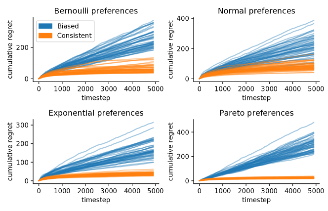
Figure 1: These plots shows the cumulative regret plotted against time for both the naive empirical averages in blue, and the unbiased averages in orange.

5.2 Personalization methods

We now focus on methods that provide more personalized recommendations. Because estimating such models is more complicated and computationally intensive, we simplify the dynamics of our simulations to a two-staged approach. We then use this approach to experiment with a feature-based and a low-rank approximation approach to personalization based on synthetically generated data.

5.2.1 Two-staged simulations

In our original setup, the platform updates its scoring rule after every observation. This is impractical when dealing with more sophisticated models. Instead we first collect a set of observations using a fixed scoring algorithm (a training set), and fit the scoring algorithm once to this training data. We then use this trained algorithm to generate a new set of observations (a test set), again without updating the algorithm in between observations. The test set is used to measure the performance of the fitted algorithm. Instead of using regret, we measure performance by directly computing the average rating on the second dataset generated by our trained algorithm. Note that it is possible to iterate generating data and fitting models multiple times before generating a test set.

5.2.2 Ridge regression

In this section we discuss a feature-based model of personalization where the rating is assumed to be a linear function of observed covariates.

The model In the feature-based setting, each item has an unknown parameter vector $w_{i}$ and each user-item pair has an observed feature vector $x_{it}$. The value of item $i$ for user $t$ then becomes

$$V_{it}=Q_{i}+x_{it}^{T}w_{i}+\theta_{it}+\varepsilon_{it}.$$ (12)

Furthermore, we also parametrize $\theta_{it}$ in terms of $x_{it}$, such that

$$\theta_{it}\sim\mathcal{N}(x_{it}^{T}\tilde{w},\sigma_{\theta})$$ (13)

where $\tilde{w}$ is another unknown parameter vector. After generating the training set using a fixed scoring rule, we use ridge regression to regress the reported ratings for each item, which leads to estimates $\hat{Q}_{i}$ and $\hat{w}_{i}$ for each item. These are then used as scoring rule: $s_{it}=\hat{Q}_{i}+x_{it}^{T}\hat{w}_{i}$.

Simulation details There are $n=100$ items, and $w_{i}\in\mathbb{R}^{p}$ where $p=20$. We generate $Q_{i}\sim\mathcal{N}(0,1)$ and $w_{ij},\tilde{w}_{ij}\sim\mathcal{N}(0,1/\sqrt{p})$ independently. The elements of the feature vectors are generated independently following $x_{ijt}\sim\mathcal{N}(0,1)$. The error term is drawn according to $\varepsilon_{it}\sim\mathcal{N}(0,1)$, and we set $\sigma_{\theta}=0.1$. We generate $10np=20000$ observations.

The training sets are generated using four different scoring rules:

1. Using the oracle scoring rule: $s_{it}=Q_{i}+x_{it}^{T}w_{i}$, which leads to perfect recommendations.

2. Using the oracle scoring rule and unbiased ratings $V_{it}-\theta_{it}$.

3. Using randomly selected items, hence the user has no choice.

4. We iterate steps one and two twice, where we first use randomly selected items, then fit a Ridge regression to estimate the parameters, and use these to generate the test set: $s_{it}=\hat{Q}_{i}+\hat{x}_{it}^{T}w_{i}$.

This last training set allows us to better understand how the system evolves over time.

Results The average values of the selected items in the test set are plotted in the left plot of Figure 2. The two dotted lines provide useful benchmarks: the top line shows the performance of the oracle scoring rule, which upper bounds the performance. The bottom line shows the performance in the absence of a scoring rule, that is $s_{it}=0$ for all $i,t$. Finally, note that random selections lead to an average rating of $0$.

We note that the best performing recommendations are given by the model trained on random data (green); these are close to the performance of the oracle. Unbiased ratings based on the oracle (orange) perform a bit worse due to a feedback loop. The model is only trained on ‘good’ selections and this leads to a degradation of performance. We also see that the iterated model (red) that was initially trained on random selections performs worse than the randomly generated data, suggesting that the quality deteriorates over time. Finally, the model trained on oracle data (blue) performs much worse than all the models, and does not perform much better than the ‘no-score algorithm’ that does not provide recommendations.

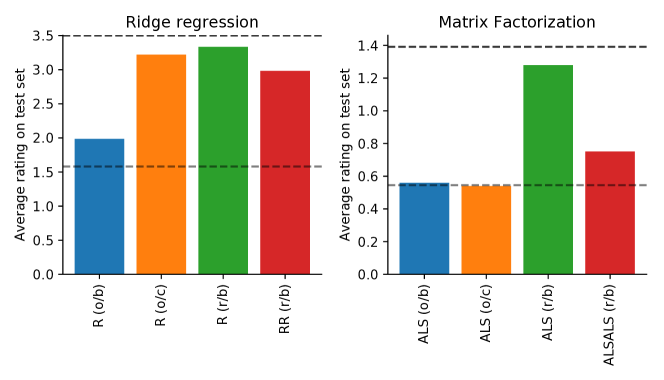
Figure 2: We compare performances of recommendation systems based on different training data in a feature-based model on the left and matrix factorization on the right. Green corresponds to random selections in the training set, orange to oracle selections with unbiased feedback, red to the iterated model initially based on random selections, and blue is based on biased oracle ratings.

5.2.3 Matrix factorization

In this section we investigate the dynamics of private preferences that are low rank. We use the same two-stage approach as before, where we first use a fixed scoring rule to generate a training set, fit our model, and use the fitted scoring rule to generate a test set to measure performance.

The model The low-rank models assumes that the value for item $i$ by user $j$ follows the model

$$v_{ij}=a_{i}+b_{j}+u_{i}^{T}v_{j}+x_{i}^{T}y_{j}+\varepsilon_{it}$$ (14)

where $u_{i}$ and $v_{j}$ are (hidden) $q$-dimensional vectors modeling interaction between user and item, and $a_{i}$ and $b_{j}$ are terms modeling overall differences between users and items. Similarly, $x_{i}$ and $y_{j}$ are $q$-dimensional vectors that combine the private preference $\theta_{it}=x_{j}^{T}y_{j}$. Note that, unlike in previous settings, here we observe the same user multiple times. The recommendation system provides score $s_{ij}$ for user $i$ and item $j$ and the user selects item

$$\arg\max_{j}s_{ij}+x_{i}^{T}y_{j}$$ (15)

and reports her value $V_{ij}$. We use alternating least squares (Koren et al., 2009) to estimate $a$, $b$, $u$ and $v$.

Simulation details As in the feature-based simulation, we generate four training sets, one based on an oracle, one based on an oracle with unbiased ratings, one based on random selections, and finally an iterated version of the random selections process, where we fit a model to the random selections data and use that model to generate training data.

We simulate 2000 users and 500 items, with rank $q=4$. Entries of $u,v,x$ and $y$ are independent Gaussians with variance $1/q$. To reduce variance, the error term has a small variance, $\varepsilon_{ij}\sim N(0,0.01)$ and for both training and test sets each user rates $40$ items. We run alternating least squares with rank $2q$ and varying regularization.

Results The two dotted lines denote the same benchmarks as before. Again, we notice that recommendations trained on random data perform best, but this time the difference is much more pronounced. The recommendations based on perfect recommendations (blue and orange) perform a lot worse. In fact, they do barely better than not recommending items at all and having users base their choice solely on their own preference signals. Part of the degradation in performance seems to be caused by a feedback loop; the observations are not randomly sampled. We also notice a much stronger degradation in performance of the iterated model (red). This suggests that the dynamic nature of recommendation systems affect matrix factorization methods more severely than the simpler linear model from the previous section.

6 Discussion

In this work, we introduce a model for analyzing feedback in recommendation systems. We propose a simple model that explicitly looks at heterogeneous preferences among users of a recommendation system, and takes the dynamics of learning into account. We then consider the consistency and efficiency of natural estimators in this model. Recent work has focused on exploration, or efficiency, with selfish agents. On the one hand, preferences lead to inconsistent estimators if this aspect is not taken into account. On the other hand, we also show that there is an upside to heterogeneous preferences; they automatically lead to efficiency. Using simulations, we demonstrate that these phenomena persist when we use more sophisticated recommendation methods, such as matrix factorization.

6.1 Future work

There are several directions of further research. Our simplified model does not capture all aspects of recommendation systems. The most interesting aspect is that, in practice, users only observe a limited set of recommendations, rather than the entire inventory. This can lead to an inefficiency in the rate of exploration, and requires further study.

Our model and simulations show that consistency of models is an issue that is difficult to resolve. We believe that progress can be made. Theoretically, one possible avenue is to also model the selection process directly and combine it with the model for outcomes. Empirically, by large scale studies that test the effects of human interaction on estimators.

6.2 The bigger picture

We believe that this work has raised fundamental and important issues relating the interaction between machine learning systems and the users interacting with them. Algorithms not only consume data, but in their interaction with users also create data, a much more opaque process but equally vital in designing systems that achieve the goals we set out to achieve. There is still a lot of room for improvement by gaining a better understanding of these dynamics.

7 Acknowledgements

This work is published in the proceedings of AISTATS 2018. The authors would like to thank Ramesh Johari, Vijay Kamble, Brad Klingenberg, Yonatan Gur, Peter Lofgren, Andrea Locatelli, and anonymous reviewers for their suggestions and feedback. This work was supported by the Stanford TomKat Center, and by the National Science Foundation under Grant No. CNS-1544548. Any opinions, findings, and conclusions or recommendations expressed in this material are those of the author(s) and do not necessarily reflect the views of the National Science Foundation.

Appendix A Appendix

Proof of Proposition 1.

We prove the result by showing that the best item cannot always be ranked at the top, because that would depress its score $s_{it}$ sufficiently much that it cannot be at the top.

Fix a sample path $\omega\in\Omega$. Note that by assumption, each arm is optimal for a constant fraction of agents. Define

$$x_{it}=\frac{|\{\tau:a_{\tau}=i\}|}{t}.$$ (16)

Then, if $\liminf_{t}x_{it}<x_{i}^{*}$ for some sufficiently small $x_{i}^{*}>0$, we incur linear regret almost surely. Instead, assume that each arm is sampled a constant fraction, $\liminf_{t}x_{it}>\delta_{i}$ for some $\delta_{i}$ for each arm $i$. We note that the expected reward for the item ranked highest is

$$Q_{i}+\frac{p}{p+(1-p)^{K}}=Q+\rho,$$ (17)

where we define $\rho=\frac{p}{p+(1-p)^{K}}$: With probability $p$ this item is chosen because of a positive signal, and with probability $(1-p)^{K}$ it is chosen because none of the items have a positive signal. For the other items, the expected reward is $Q_{i}+1$.

To understand limiting behavior of the item scores, it is thus important to understand how often an item is ranked first by the platform. Define $c_{t}$ as the fraction (up to time $t$) that the first (best) item is not ranked at the top:

$$c_{t}=\frac{|\{\tau<t:\exists j>1:s_{1\tau}<s_{j\tau}\}|}{t}.$$ (18)

We note that if $\limsup_{t}c_{t}>c^{*}$ for some $c^{*}>0$, then the regret is linear.

Informally, we proceed by bounding $\mathbb{P}(\text{item is ranked first}\mid\text{item is selected})$, and use that to understand the evolution of the averages of ratings the platform observes. To bound the above probability, we note that there are two extremes when the item is not ranked first; it is ranked second, or ranked last. If it is always ranked second when the item is not ranked first, it is less likely the item was ranked first given selection than when it is either ranked first or last. If, overall, the item is ranked first with fraction $y$, then we obtain

$$\lambda(y)\leq\mathbb{P}(\text{item ranked first}\mid\text{item selected})\leq\lambda^{\prime}(y)$$ (19)

where

$$\lambda(y)=\frac{y(p+(1-p)^{K})}{y(p+(1-p)^{K})+(1-y)p(1-p)},$$ (20)

and

$$\lambda^{\prime}(y)=\frac{y(p+(1-p)^{K})}{y(p+(1-p)^{K})+(1-y)p(1-p)^{K-1}}$$ (21)

correspond to the two extreme cases. Note that $\lambda$ and $\lambda^{\prime}$ are both decreasing.

Now suppose $\limsup c_{t}=c$. By the stong law of large numbers, the empirical average converges to its mean and thus

$$\limsup_{t}s_{1t}\leq Q_{1}+\lambda(1-c)\rho+(1-\lambda(1-c)),$$ (22)

where the second term corresponds to the expected reward from being ranked first and the last term corresponds to the contribution from when the action is not ranked first. Similarly

$$\liminf_{t}s_{2t}\geq Q_{2}+\lambda^{\prime}(c)\rho+(1-\lambda^{\prime}(c)),$$ (23)

almost surely by the mean-converging condition.

We note for $c=0$, this leads to

$$\limsup_{t}s_{1t}\leq Q_{1}+\rho\text{ and }\liminf_{t}s_{2t}\geq Q_{2}+1$$ (24)

This is a contradiction if $\Delta<\frac{(1-p)^{K}}{p+(1-p)^{K}}$, as this would imply the score of the second arm is higher in the limit than that of the first arm, while the first item is always ranked before the second item ($c=0$):

$$\limsup_{t}s_{1t} =Q_{2}+\Delta+\rho$$ (25)

$$<Q_{2}+\frac{(1-p)^{K}}{p+(1-p)^{K}}+\frac{p}{p+(1-p)^{K}}$$ (26)

$$\leq\liminf_{t}s_{2t}.$$ (27)

Furthermore, since $\lambda$ and $\lambda^{\prime}$ are continuous and monotone, there must exist some $c^{*}\in(0,1)$ such that

$$Q_{1}+\lambda(1-c^{*})\rho+1-\lambda(1-c^{*})\leq\\ Q_{2}+\lambda^{\prime}(c^{*})+1-\lambda^{\prime}(c^{*})$$ (28)

almost surely. Thus, if the first item is the top ranked item fracion $1-c^{*}$ of the time, then its score is almost surely lower than the second item, which is a contradiction. This implies that $\limsup_{t}c_{t}>c^{*}$ almost surely, which proves that the regret is linear. ∎

Proof Proposition 2.

To bound the regret, we look at individual arms and note that if at time $t$ all scores $s_{it}$ are reasonably accurate, i.e. $|s_{it}-Q_{i}|<\lambda$ for all $i$, at such time the regret is at most $2\lambda$. Furthermore, if $\lambda<\frac{\Delta_{\min}}{2}$, then the regret is $0$ as each agent is compelled to pick the best item for them. Finally, it is important to note that the regret at each period is at most $2$.

We proceed as follows; we use concentration to bound the estimation error when we have observed enough sample values. Furthermore, we show that due to natural exploration, we have a high probability guarantee of observing samples for each item. When combined, they lead to a logarithmic regret bound.

To use a concentration bound on the estimation error, we define event

$$A_{m}(i,\lambda)=\left\{\exists s\in\{m,\ldots,T\}:\frac{1}{s}\left|\sum_{j=1}^{s}\varepsilon_{ij}\right|>\lambda\right\}.$$ (29)

That is, $A_{m}(i,\lambda)$ is the bad event that after $m$ pulls, there is some time $t$ that the score $s_{it}$ is off by more than $\lambda$.

Furthermore, we define events

$$B_{m}(i,M)=\left\{|S|<m:\tau\in S\iff a_{\tau}=i\text{ and }\tau<M\right\}$$ (30)

that indicate whether within $M$ time steps, at least $m$ users reported values for item $i$.

Using these two events, we can bound the expected regret by

$$\mathbb{E}[\textup{regret}(T)]\leq\sum_{i=1}^{K}2(\mathbb{P}(A_{m}(i,\lambda))+\mathbb{P}(B_{m}(i,M)))T\\ +2M+\lambda T{\mathbb{I}}_{\lambda>\frac{\Delta_{\min}}{2}}$$ (31)

Bounding $A_{m}$ Using the standard $\sigma$-sub-Gaussian concentration bound (see, for example, Wainwright [2015, Chapter 2]), we have

$$\mathbb{P}(A_{m}(i,\lambda)) \leq\mathbb{P}\left(\exists s\in\{m,\ldots,t\}:\frac{1}{s}\left|\sum_{i=1}^{s}\varepsilon_{i}\right|>\lambda\right)$$ (32)

$$\leq\sum_{s=m}^{t}\mathbb{P}\left(\frac{1}{s}\left|\sum_{i=1}^{s}\varepsilon_{i}\right|>\lambda\right)$$ (33)

$$\leq 2\sum_{s=m}^{t}\exp\left(-\frac{s\lambda^{2}}{2\sigma^{2}}\right)$$ (34)

$$\leq 2\int_{m}^{t+1}\exp\left(-\frac{s\lambda^{2}}{2\sigma^{2}}\right)ds$$ (35)

$$\leq\frac{4\sigma^{2}}{\lambda^{2}}\exp\left(-\frac{m\lambda^{2}}{2\sigma^{2}}\right)$$ (36)

Now set

$$m=\frac{2\sigma^{2}(\log(T)-\log(\lambda))}{\lambda^{2}},$$ (37)

and obtain

$$\mathbb{P}(A_{m}(i,\lambda))\leq\frac{4\sigma^{2}}{\lambda^{2}}\exp\left(-\frac{m\lambda^{2}}{2\sigma^{2}}\right)=\frac{4\sigma^{2}}{\lambda T}$$ (38)

Bounding $B_{m}$ From the above, we know that the estimation error concentrates well after observing $m$ selections. Now we show that with high probability, it does not take too long to wait for $m$ selections.

First note that the probability of selection of any item at any time $t$ is at least $2^{1-K}\gamma$. This follows from the conditions imposed on $F_{i}$. For $M>m$, we note that the probability that we have not observed $m$ selections is lower bounded by a Binomial random variable $Z\sim B(M,2^{1-K}\gamma)$ since preferences are independent between agents. Consider

$$M=\frac{2\alpha m}{2^{1-K}\gamma}=\frac{4\alpha\sigma^{2}(\log(T)-\log(\lambda))}{\lambda^{2}2^{1-K}\gamma}$$ (39)

where $\alpha=\max\left(1,2\lambda^{2}/\sigma^{2}\right)$ .

First we note that in this case, $\mathbb{E}(Z)=2\alpha m\geq 2m$ and thus

$$\mathbb{P}(B_{m}) \leq\mathbb{P}\left(Z\leq\frac{1}{2}\mathbb{E}(Z)\right)$$ (40)

$$\leq\exp\left(-\frac{\mathbb{E}(Z)}{8}\right)$$ (41)

$$\leq\exp\left(-\frac{\alpha\sigma^{2}(\log(T)-\log(\lambda))}{2\lambda^{2}}\right)$$ (42)

$$\leq\frac{\lambda}{T}$$ (43)

where third inequality is a standard Chernoff bound and the second to last step follows from the condition on $\alpha$.

Plugging these bounds on $A_{m}(i,\lambda)$ and $B_{m}(i,M)$ in to our bound for regret (31), we obtain

$$\begin{split}\mathbb{E}[\textup{regret}(T)]&\leq 2\left(\frac{4\sigma^{2}}{\lambda}+\lambda\right)K\\ &+\frac{8\alpha\sigma^{2}K(\log(T)-\log(\lambda))}{\lambda^{2}2^{1-K}\gamma}+\lambda KT{\mathbb{I}}_{\lambda>\frac{\Delta_{\min}}{2}}\end{split}$$ (44)

and thus if we set $\lambda=\frac{\Delta_{\min}}{2}$, we find

$$\begin{split}\mathbb{E}[\textup{regret}(T)]&\leq\left(\frac{16\sigma^{2}}{\Delta_{\min}}+\Delta_{\min}\right)K\\ &+\frac{32\alpha\sigma^{2}K(\log(T)-\log(\Delta_{\min})+\log(2))}{\Delta_{\min}^{2}2^{1-K}\gamma}\end{split}$$ (45)

as desired. ∎

References

- Adomavicius and Tuzhilin [2005] Gediminas Adomavicius and Alexander Tuzhilin. Toward the next generation of recommender systems: A survey of the state-of-the-art and possible extensions. IEEE Trans. Knowl. Data Eng., 17:734–749, 2005.
- Amatriain et al. [2009] Xavier Amatriain, Josep M Pujol, and Nuria Oliver. I like it… i like it not: Evaluating user ratings noise in recommender systems. In International Conference on User Modeling, Adaptation, and Personalization, pages 247–258. Springer, 2009.
- Auer et al. [2002] Peter Auer, Nicolò Cesa-Bianchi, and Paul Fischer. Finite-time analysis of the multiarmed bandit problem. Machine Learning, 47:235–256, 2002.
- Bastani et al. [2017] Hamsa Bastani, Mohsen Bayati, and Khashayar Khosravi. Exploiting the natural exploration in contextual bandits. arXiv preprint arXiv:1704.09011, 2017.
- Bubeck and Cesa-Bianchi [2012] Sébastien Bubeck and Nicolò Cesa-Bianchi. Regret analysis of stochastic and nonstochastic multi-armed bandit problems. CoRR, abs/1204.5721, 2012.
- Camerer [1998] Colin Camerer. Bounded rationality in individual decision making. Experimental economics, 1(2):163–183, 1998.
- Chamley [2004] C. Chamley. Rational Herds: Economic Models of Social Learning. Rational Herds: Economic Models of Social Learning. Cambridge University Press, 2004. ISBN 9780521530927. URL https://books.google.com/books?id=2dgbOh6VE9YC.
- Demarzo et al. [2003] Peter M Demarzo, Dimitri Vayanos, Jeffrey Zwiebel, Nick Barberis, Gary Becker, Jonathan Bendor, Larry Blume, Simon Board, Eddie Dekel, Stefano Dellavigna, Darrell Duffie, David Easley, Glenn Ellison, Simon Gervais, Ed Glaeser, Ken Judd, David Kreps, Edward Lazear, George Loewenstein, Lee Nelson, Anthony Neuberger, Matthew Rabin, José Scheinkman, Antoinette Schoar, Peter Sorenson, Pietro Veronesi, and Richard Zeckhauser. Persuasion bias, social influence, and unidimensional opinions. 2003.
- Ellison and Fudenberg [1993] Glenn Ellison and Drew Fudenberg. Rules of thumb for social learning. Journal of Political Economy, 101(4):612–643, 1993.
- Ellison and Fudenberg [1995] Glenn Ellison and Drew Fudenberg. Word-of-mouth communication and social learning. The Quarterly Journal of Economics, 110(1):93–125, 1995.
- Frazier et al. [2014] Peter I. Frazier, David Kempe, Jon M. Kleinberg, and Robert Kleinberg. Incentivizing exploration. In SIGECOM, 2014.
- Hummel and McAfee [2014] Patrick Hummel and R. Preston McAfee. Machine learning in an auction environment. In WWW, 2014.
- Ifrach et al. [2014] Bar Ifrach, Costis Maglaras, and Marco Scarsini. Bayesian social learning with consumer reviews. SIGMETRICS Performance Evaluation Review, 41:28, 2014.
- Joachims et al. [2017] Thorsten Joachims, Adith Swaminathan, and Tobias Schnabel. Unbiased learning-to-rank with biased feedback. CoRR, abs/1608.04468, 2017.
- Kahneman [2003] Daniel Kahneman. Maps of bounded rationality: Psychology for behavioral economics. The American economic review, 93(5):1449–1475, 2003.
- Koren et al. [2009] Yehuda Koren, Robert M. Bell, and Chris Volinsky. Matrix factorization techniques for recommender systems. Computer, 42, 2009.
- Kremer et al. [2013] Ilan Kremer, Yishay Mansour, and Motty Perry. Implementing the ”wisdom of the crowd”. In SIGECOM, 2013.
- Liu et al. [2015] Tie-Yan Liu, Wei Chen, and Tao Qin. Mechanism learning with mechanism induced data. In AAAI, pages 4037–4041, 2015.
- Mackey et al. [2010] Lester W. Mackey, David J. Weiss, and Michael I. Jordan. Mixed membership matrix factorization. In ICML, 2010.
- Mansour et al. [2015] Yishay Mansour, Aleksandrs Slivkins, and Vasilis Syrgkanis. Bayesian incentive-compatible bandit exploration. CoRR, abs/1502.04147, 2015.
- Mansour et al. [2016] Yishay Mansour, Aleksandrs Slivkins, Vasilis Syrgkanis, and Zhiwei Steven Wu. Bayesian exploration: Incentivizing exploration in bayesian games. In Proceedings of the 2016 ACM Conference on Economics and Computation, EC ’16, pages 661–661, New York, NY, USA, 2016. ACM. ISBN 978-1-4503-3936-0. doi: 10.1145/2940716.2940755. URL http://doi.acm.org/10.1145/2940716.2940755.
- Marlin [2003] Benjamin M. Marlin. Modeling user rating profiles for collaborative filtering. In NIPS, 2003.
- Marlin et al. [2007] Benjamin M. Marlin, Richard S. Zemel, Sam T. Roweis, and Malcolm Slaney. Collaborative filtering and the missing at random assumption. In UAI, 2007.
- Papanastasiou et al. [2014] Yiangos Papanastasiou, Kostas Bimpikis, and Nicos Savva. Crowdsourcing exploration. History, 2014.
- Qiang and Bayati [2016] Sheng Qiang and Mohsen Bayati. Dynamic pricing with demand covariates. 2016.
- Russo and Roy [2016] Daniel Russo and Benjamin Van Roy. An information-theoretic analysis of thompson sampling. Journal of Machine Learning Research, 17:68:1–68:30, 2016.
- Schnabel et al. [2016] T. Schnabel, A. Swaminathan, A. Singh, N. Chandak, and T. Joachims. Recommendations as Treatments: Debiasing Learning and Evaluation. ArXiv e-prints, February 2016.
- Smith and Sørensen [2000] Lones Smith and Peter Sørensen. Pathological outcomes of observational learning. Econometrica, 68(2):371–398, 2000.
- Steck [2010] Harald Steck. Training and testing of recommender systems on data missing not at random. In KDD, 2010.
- Wainwright [2015] Martin Wainwright. High-dimensional statistics: A non-asymptotic viewpoint. Forthcoming, 2015.