Instantaneous Pairing of Lyapunov Exponents in Chaotic Hamiltonian Dynamics and the 2017 Ian Snook Prizes ;
Short Running-Head Title for CMST :
2017 Snook Prizes : How Lyapunov Exponents Pair

Abstract

The time-averaged Lyapunov exponents, $\{\ \lambda_{i}\ \}$, support a mechanistic description of the chaos generated in and by nonlinear dynamical systems. The exponents are ordered from largest to smallest with the largest one describing the exponential growth rate of the ( small ) distance between two neighboring phase-space trajectories. Two exponents, $\lambda_{1}+\lambda_{2}$, describe the rate for areas defined by three nearby trajectories. $\lambda_{1}+\lambda_{2}+\lambda_{3}$ is the rate for volumes defined by four nearby trajectories, and so on. Lyapunov exponents for Hamiltonian systems are symmetric. The time-reversibility of the motion equations links the growth and decay rates together in pairs. This pairing provides a more detailed explanation than Liouville’s for the conservation of phase volume in Hamiltonian mechanics. Although correct for long-time averages, the dependence of trajectories on their past is responsible for the observed lack of detailed pairing for the instantaneous “local” exponents, $\{\ \lambda_{i}(t)\ \}$ . The 2017 Ian Snook Prizes will be awarded to the author(s) of an accessible and pedagogical discussion of local Lyapunov instability in small systems. We desire that this discussion build on the two nonlinear models described here, a double pendulum with Hooke’s-Law links and a periodic chain of Hooke’s-Law particles tethered to their lattice sites. The latter system is the $\phi^{4}$ model popularized by Aoki and Kusnezov. A four-particle version is small enough for comprehensive numerical work and large enough to illustrate ideas of general validity.

I Introduction

The elucidation of Hamiltonian chaos and Lyapunov instability by Poincaré and Lorenz is familiar textbook material. Models which capture aspects of complexity, the Logistic and Baker Maps, the Lorenz attractor and the Mandelbrot Set, combine visual appeal with mechanistic understanding in the bare minimum of spatial dimensions, two for maps and three for flows. Mechanical models with only three- or four-dimensional phase spaces are simple enough that the entire phase space can be explored exhaustively.“Small Systems” can augment our understanding of nature in terms of numerical models by introducing more complexity. Just a few more degrees of freedom make an ergodic exhaustive sampling impossible. For the small systems we treat here we take on the more difficult task of defining and analyzing the time-dependent convergence of “typical” trajectories.

Chaos involves the exponential growth of perturbations. Joseph Ford emphasized the consequence that the number of digits required in the initial conditions is proportional to the time for which an accurate solution is desired. Accordingly a “typical” nonexhaustive trajectory or history is the best that we can do. To go beyond the simplest models to those which elucidate macroscopic phenomena, like phase transitions and the irreversibility described by the Second Law of Thermodynamics, we like Terrell Hill’s idea of small-system studies ( in the 1960s he wrote a prescient book, Thermodynamics of Small Systems. ) In what follows we describe two small-system models which are the foci of the Ian Snook Prize Problem for 2017. These models are Hamiltonian, both with four degrees of freedom so that their motions are described in eight-dimensional phase spaces.

Figure 1: Snapshots of the two springy pendulum masses at times of 2, 4, 6, and 8. Initially the pendulum is horizontal as at the top right. The initial configuration has vanishing energy. Only the outermost particle, Particle 2, responds to the vertical gravitational field.

I.1 The Springy Pendulum and the Springy Double Pendulum

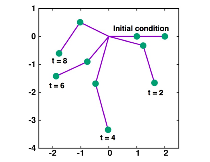
The double pendulum with rigid links is an excellent model for the table-top demonstration of chaos. Bill saw one in action at an all-day Stanford lecture given by James Yorke. An even simpler mathematical model for chaos can be obtained with a single pendulum. For chaos the single pendulum needs a spring rather than a rigid link. The single springy pendulum moves in a four-dimensional phase space, just as does the double pendulum with rigid links. Along with Harald Poschb1 ; b2 we investigated mathematical models for chaos based on chains of pendula, both rigid and springy. We studied many-body instabilities by characterizing the form of the detailed description of many-dimensional chaos, the Lyapunov spectrum. We considered two kinds of model Hamiltonians describing chains in a gravitational field : [ 1 ] chains composed of particles with equal masses, as in a physical length of chain; [ 2 ] chains in which only the bottom mass was affected by gravity, as in a light chain supporting a heavy weight. Figure 1 shows five snapshots, equally spaced in time, from a chaotic double-pendulum trajectory. Initially the motionless chain was placed in the horizontal configuration appearing at the top right of Figure 1. If gravity affects only the lower of the two masses ( as in the type-2 models supporting a heavy weight ) the corresponding Hamiltonian is

$${\cal H}=[\ p_{1}^{2}+p_{2}^{2}\ ]/2+(\kappa/2)[\ (r_{1}-1)^{2}+(r_{12}-1)^{2}\ ]+y_{2}\ .$$

where $r_{1}$ and $r_{12}$ are the lengths of the upper and lower springs. To enhance the coupling between the springs and gravity we choose the force constant $\kappa=4$ here.

I.2 The Spectrum of Time-Averaged Lyapunov Exponents, $\{\ \lambda\ \}$

The Lyapunov exponents making up the spectrum are conventionally numbered in the descending order of their long-time-averaged values. We begin with the largest, $\lambda_{1}$ . $\lambda_{1}$ describes the long-time-averaged rate at which the distance between the trajectories of two nearby phase-space points increases. That rate, $\lambda_{1}\equiv\langle\ \lambda_{1}(t)\ \rangle\equiv\langle\ (d\ln\delta/dt)\ \rangle$ , is necessarily positive in a chaotic system. A more detailed description of rates of change of lengths and areas, and volumes, and hypervolumes of dimensionality up to that of the phase space itself, leads to definitions of additional Lyapunov exponents. The next exponent, $\lambda_{2}$ , is needed to describe the rate at which a typical phase-space area, defined by three nearby points, increases ( or decreases ) with increasing time, $\lambda_{1}+\lambda_{2}\equiv\langle\ (d\ln A/dt)\ \rangle=\langle\ \lambda_{1}(t)+\lambda_{2}(t)\ \rangle\$. Again an average over a sufficiently long time for convergence is required. Likewise the time-averaged rate of change of a three-dimensional phase volume defined by four neighboring trajectories is $\lambda_{1}+\lambda_{2}+\lambda_{3}$ . This sequence of rates and exponents continues for the rest of the spectrum. There are $D$ exponents for a $D$-dimensional phase-space description.

I.3 Local and Global Lyapunov-Exponent “Pairing” for Hamiltonian Systems

The time-reversibility of Hamiltonian mechanics implies that all the rates of change change sign if the direction of time is reversed. This suggests, for instance, that all the exponents, $\{\ \lambda\ \}$ and $\{\ \lambda(t)\ \}$ , are “paired”, with the rates forward in time opposite to those backward in time. This turns out to be “true” for the long-time-averaged exponents but could be “false” for the local exponents. Local exponents depend upon the recent past history of neighboring trajectories. The global exponents, which describe the growth and decay of the principal axes of comoving hyperellipsoids in phase space are paired, though the time required to show this through numerical simulation can be long. This exponent pairing is the focus of the 2017 Snook Prize, as we detail in what follows. There is a vast literature describing and documenting the numerical evaluation and properties of Lyapunov spectra. The theoretical treatments are sometimes abstruse and lacking in numerical verification. This year’s Prize Problem seeks to help remedy this situation. The numerical foundation for the study of Lyapunov exponents is an algorithm developed by Shimada and Nagashima in Sapporob3 and Benettin in Italy, along with his colleagues Galgani, Giorgilli, and Strelcynb4 , beginning in the late 1970s. Google indicates hundreds of thousands of internet hits for “Lyapunov Spectrum”. We mention only a few other referencesb5 ; b6 ; b7 ; b8 here. The internet makes these and most of the rest readily available.

I.4 The $\phi^{4}$ Model for Chaos and Heat Conduction in Solids

Figure 2: The four-body $\phi^{4}$ chain can be pictured as an infinitely-long chain with a four-particle unit cell ( shown in red ), or as an arrangement of masses on a circle with equally-spaced lattice sites to which the particles are tethered. It is convenient ( but not foolproof ) to choose an initial condition with velocities $\{\ +v,+v,+v,-v\ \}\ {\rm or}\ \{\ +2v,0,0,0\ \}\longrightarrow(E/N)=(v^{2}/2)\ .$ The initial conditions $\{\ +v,+v,-v,-v\ \}\ {\rm and}\ \{\ +v,-v,+v,-v\ \}$ are “normal modes”, discussed at length in References 10 and 11.

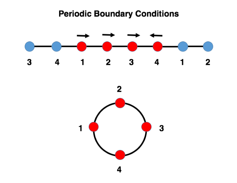
Aoki and Kusnezov popularized the $\phi^{4}$ model as a prototypical atomistic lattice-based model leading to Fourier heat conductionb9 ; b10 ; b11 . In addition to a nearest-neighbor Hooke’s-Law potential the model incorporates quartic tethers binding each particle to its own lattice site.

Here we denote the displacements of the particles from their sites as $\{\ q_{i}\ \}$ . In our one-dimensional case the spacing between the lattice sites does not appear in the Hamiltonian or in the equations of motion. In numerical work it is convenient to choose the spacing equal to zero while setting the particle masses, force constants for the pairs, and those for the tethers all equal to unity. For a four-particle problem in an eight-dimensional phase space the three-part Hamiltonian is :

$${\cal H}=\sum_{i=1}^{4}[\ (p_{i}^{2}/2)+(q_{i}^{4}/4)\ ]+\sum_{4}^{springs}(q_{i,j}^{2}/2)\ .$$

The periodic boundary condition includes the spring linking particles 1 and 4 :

$$\ddot{q}_{1}=-q_{1}^{3}+q_{2}+q_{4}-2q_{1}\ ;\ \ddot{q}_{4}=-q_{4}^{3}+q_{1}+q_{3}-2q_{4}\ .$$

See Figure 2 for two ways of visualizing the periodic boundary conditions of the $\phi^{4}$ chain.
The energy range over which chaos is observed in the $\phi^{4}$ model includes about nine orders of magnitudeb10 ; b11 . The chaotic range for a four-body chain includes the two cases we discuss in the present work, $\{\ E=8,\ 288\ ;\ (E/N)=2,\ 72\ \}$ . With both the springy pendulum and the $\phi^{4}$ models in mind we turn next to a description of their chaotic properties.

II The Chaotic Dynamics of the Springy Double Pendulum

Like most smoothly-differentiable Hamiltonian systems the double springy pendulum has infinitely many periodic or quasiperiodic phase-space solutions surrounded by a chaotic sea. Dynamics in the sea is exponentially sensitive to perturbations. The dynamics occurs in an eight-dimensional phase space. Perturbations oriented along the trajectory or perpendicular to the energy surface, where there is no longtime growth at all, give two zeroes, so that the maximum number of nonzero Lyapunov exponents is six.

Each positive exponent is necessarily paired with its negative twin, with the two changing roles if the direction of time is reversed. It is often stated that this time-reversible pairing links not only the time-averaged rates of the dynamics, but also the “local” or “instantaneous” ratesb2 . Because chaotic pendulum problems give different local exponents if Cartesian and polar coordinates are used one might think that pairing could be hindered by using a mixture of these coordinates. To check on this idea we considered a mixed-coordinate Hamiltonian for the model of Figure 1 with polar coordinates for the “inside” Particle 1 :

$${\cal H}=(1/2)[\ p_{r}^{2}+(p_{\theta}/r)^{2}+p_{x}^{2}+p_{y}^{2}\ ]+y_{2}+(\kappa/2)[\ (r-1)^{2}+(r_{12}-1)^{2}\ ]\ ;$$

$$r_{12}=\sqrt{x_{2}^{2}+y_{2}^{2}+r_{1}^{2}-2r_{1}x_{2}\sin(\theta_{1})+2r_{1}y_{2}\cos(\theta_{1})}\ ;\ \kappa=4\ .$$

Formulating and solving the motion equations in mixed Cartesian and polar coordinates is an intricate error-prone task. It is useful first to solve the problem in Cartesian coordinates. That solution then provides a check for the more complicated mixed-coordinate case. Energy conservation is a nearly-infallible check of the programming. We computed spectra of Lyapunov exponents averaged over one billion fourth-order and one billion fifth-order Runge-Kutta timesteps, $dt=0.001$ . This ensures that the numerical truncation errors of order $(dt^{5}/120)$ or $(dt^{6}/720)$ are of the same order as the double-precision roundoff error. We chose the initial condition of Figure 1 with both masses motionless at the support level, $\{\ x_{1},y_{1},x_{2},y_{2}\ \}=\{\ 1,0,2,0\ \}$ , so that the initial potential, kinetic, and total energies all vanished. Only the outer Cartesian mass interacts with the gravitational field.

The simplest numerical method for obtaining Lyapunov spectrab3 ; b4 is first to generate a $D$-dimensional “reference trajectory” in the $D$-dimensional phase space. Then a set of $D$ similar “offset” trajectories, an infinitesimal distance away, $\delta$ , are generated in the same space with numerical offset vectors of length $\delta=0.00001$ or 0.000001. While advancing the resulting $D(D+1)$ $D$-dimensional differential equations the local Lyapunov exponents are obtained by “Gram-Schmidt” orthonormalization. This process rescales the vectors to their original length and rotates all but the first of them in order to maintain their orthonormal arrangement. The rescaling operation portion of the Gram-Schmidt process gives local values for the $D$ Lyapunov exponents :

$$\lambda_{i}(t)\equiv(-1/dt)\ln(\delta_{i}^{after}/\delta_{i}^{before})\ ;\ \lambda_{i}\equiv\langle\ \lambda_{i}(t)\ \rangle\ .$$

For the type-2 double pendulum of Figure 1 the time-averaged Lyapunov spectrum is :

$$\{\ \lambda\ \}=\{\ +0.143,+0.076.+0.034,0.000,0.000,-0.034,-0.076,-0.143\ \}\ .$$

The rms fluctuations in these rates are typically orders of magnitude larger than the rates themselves. The uncertainty in the exponents as well as the differences between exponents using fourth-order or fifth-order Runge-Kutta integrators with $dt=0.001$ are both of order $\pm 0.001$ . Our numerical work shows that the pairing of the exponents is maintained if one of the pendula is described by polar coordinates with the other pendulum Cartesian. The local exponents are different but still paired.

Figure 3: Typical pairing (a) of the eight Lyapunov exponents for the double-pendulum problem using Cartesian coordinates stored in the order $\{\ (x,y,p_{x},p_{y})_{1},(x,y,p_{x},p_{y})_{2}\ \}$ , with the $i$th offset vector initially parallel to the $i$th member of this set of variables. Typical equilibrating pair sums $\{\ \lambda_{i}(t)+\lambda_{9-i}(t)\ \}$ are also shown in (b). Fourth-order double-precision Runge-Kutta integration was used with a timestep $dt=0.001$ and offset vectors of length $\delta=0.000001$ . The initial condition is that shown in Figure 1.

III Convergence and Ordering of Local Lyapunov Exponents

The algorithm for generating the Lyapunov exponentsb3 ; b4 requires the ordering of $D$ offset vectors in the vicinity of a reference trajectory. The first vector follows exactly the same motion equations with the proviso that its length is constant. The second vector, also of constant length, is additionally required to remain orthogonal to the first so that the combination of the two gives the rate of expansion or contraction of two-dimensional areas in the vicinity of the reference trajectory. In general the $n$th offset vector satisfies $n$ constraints in all, keeping its own length constant while also maintaining its orthogonality to the preceding $n-1$ vectors.

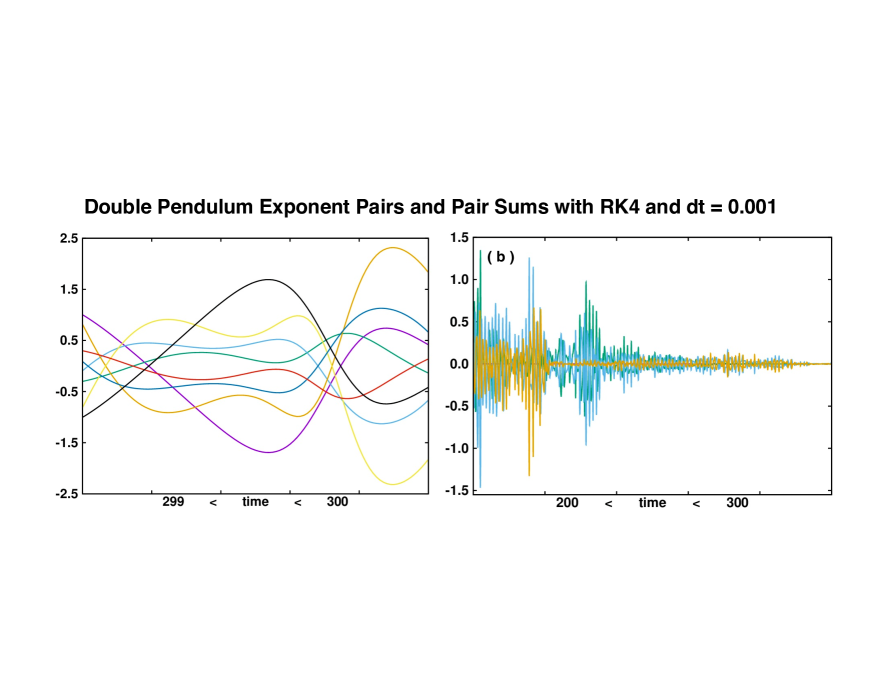
Although the local rates $\{\ \lambda(t)\ \}$ associated with the vectors are necessarily ordered when time-averaged over a sufficiently long time to give the $\{\ \lambda\ \}$ , this ordering is regularly violated, locally, as Figures 3 and 4 show. Offhand one would expect that increasing the Lyapunov exponents or decreasing the accuracy of the simulation would lead to more rapid convergence of the ordering of the vectors. For this reason we consider a model which is as simple as possible, with a relatively large chaotic range, and is easy to simulate. This $\phi^{4}$ model, named for its quartic tethering potential, has proved particularly useful in the simulation of heat flow. We consider the equilibrium version of the model here, an isolated system.

IV The Dynamics of One-Dimensional Periodic $\phi^{4}$ Models

Figure 4: Evolution ( a ) of the cumulative Lyapunov spectrum for the $\phi^{4}$ model from the initial condition $\{\ p\ \}=\{\ 2,2,2,-2\ \}$ with $dt=0.001$ and the offset length $\delta=0.000001$ . Simulations using RK4 or RK5 in either phase space or in tangent space all “look” similar in this time range. Evolution ( b ) of the Lyapunov spectrum over a longer time range showing pairing using RK4. Results were calculated using Karl Travis’ FORTRAN 90 computer program in the $\phi^{4}$ phase space.

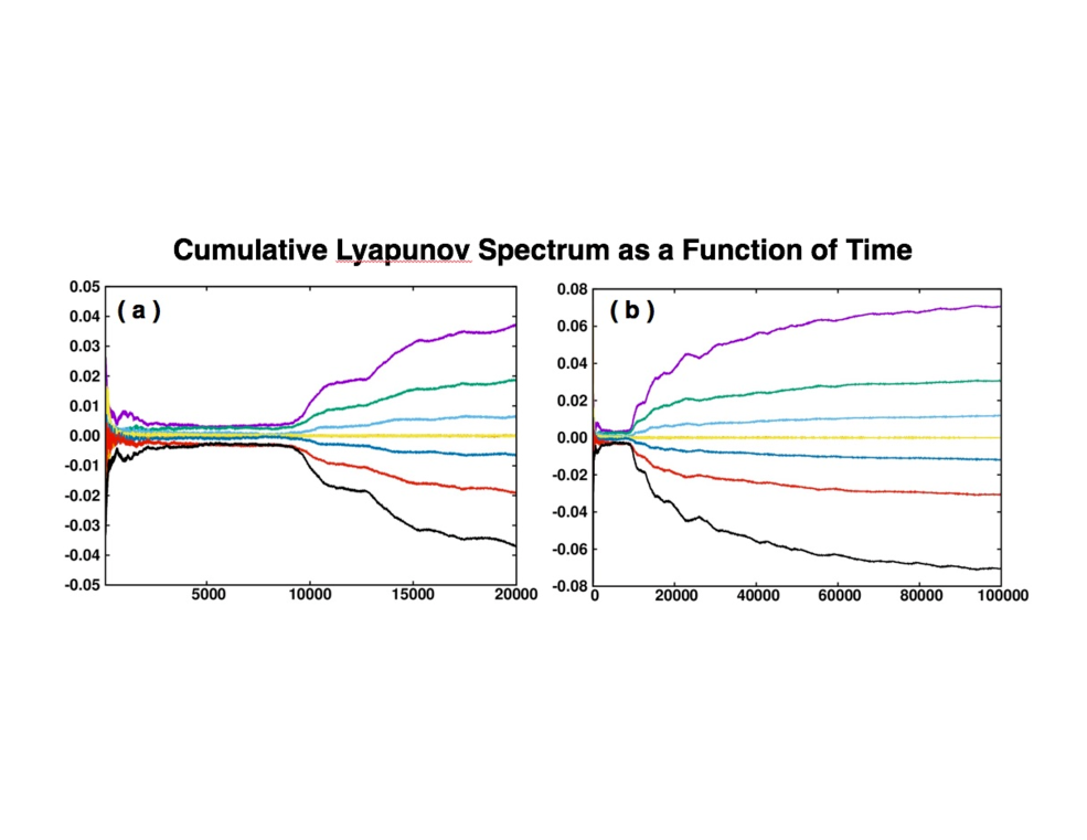
The simplest Lyapunov algorithm for the $\phi^{4}$ model is exactly that used with the springy pendula. We follow $D+1$ trajectories in the $D$-dimensional phase space, rescaling them at every timestep to obtain the complete spectrum of $D=8$ instantaneous Lyapunov exponents. This phase-space integration of nine trajectories, followed by Gram-Schmidt orthonormalization, can be modified by using Lagrange multipliers to impose the eight constant-length constraints and the $(1/2)(8\cdot 7)=28$ orthogonality constraints. A third approach, particularly simple to implement for the $\phi^{4}$ model with its power-law equations of motion, is to linearize the motion equations so that the offset vectors, rather than being small, can be taken as unit vectors in “tangent space”. By using separate integrators for the “reference trajectory” and for the eight unit vectors the programming is at about the same level of difficulty as is that of the straightforward phase-space approach. We implemented both approaches for the $\phi^{4}$ problems and found good agreement for the Lyapunov spectra at a visual level, even for calculations using a billion timesteps. This is because the reference trajectories for the phase-space and tangent-space algorithms are identical.

V Useful Integration Techniques

Figure 5: We illustrate the dependence of integration errors ( RK4 versus RK5 ) for low energy and higher-energy $\phi^{4}$ chains with initial values $\{\ q\ \}=\{\ 0,0,0,0\ \}$ with $\{\ p\ \}=\{\ 2,2,2,-2\ \}\ {\rm and}\ \{\ 12,12,12,-12\ \}$ respectively. After a linear induction period the errors grow exponentially, reflecting Lyapunov instability, until saturation.

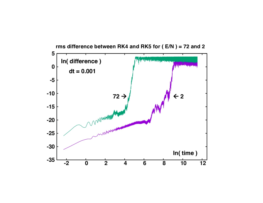
Fourth-order and fifth-order Runge-Kutta integrators are particularly useful algorithms for small systems. First, these integrators are easy to program. These integrators are also explicit, a real simplification whenever a variable timestep is desirable. Their errors are typically opposite in sign. For the simple harmonic oscillator the fourth-order energy decays while the fifth-order energy diverges. By choosing a sufficiently small timestep, for which the two algorithms agree, one can be confident in the accuracy of the trajectories. Another useful technique is adapative integration : comparing solutions with a single timestep $dt$ to those from two successive half steps with $(dt/2)$. The timestep is then adjusted up or down by a factor of two whenever it is necessary to keep the root-mean-squared error in a prescribed band, $10^{-12}>{\tt error}>10^{-14}$ for instance.b12

At the expense of about a factor of fifty in computer time, FORTRAN makes it possible to carry out quadruple-precision simulations with double-precision programming by changing the gnu compiler command :

$${\tt gfortran}\ {\rm-}{\tt O}\ {\rm-}{\tt o}\ {\tt xcode}\ {\tt code.f}\longrightarrow{\tt gfortran}\ {\rm-}{\tt O}\ {\rm-}{\tt o}\ {\tt xcode}\ {\tt-}{\tt freal}{\rm-}{\tt 8}{\rm-}{\tt real}{\rm-}{\tt 16\ code.f}$$

Here the FORTRAN program is code.f and the executable is xcode .

VI The 2017 Ian Snook Prize Problem

The springy pendula and $\phi^{4}$ problems detailed here show that “pairing” is typically present after sufficient time, with that time sensitive to the largest Lyapunov exponent as well as to the initial conditions. There are several features of these introductory problems that merit investigation :
[ 1 ] To what extent is there an unique chaotic sea ? Can the symmetry of the initial conditions limit the portion of phase space visited when the dynamics is chaotic ?
[ 2 ] Within the $\phi^{4}$ model’s chaotic sea do the time-averaged kinetic temperatures $\{\ T_{i}=\langle\ p_{i}^{2}\ \rangle\ \}$ , agree for all the particles ? ( If not, a thermal cycle applying heat and extracting work from the chain could be developed so as to violate the Second Law.b11 )
[ 3 ] Is the pairing time simply related to the Lyapunov exponents and the chain length ?
[ 4 ] Is the accuracy of the pairing simply related to the accuracy of the integrator ?
The next and last question, which motivated this year’s Prize Problem seems just a bit more difficult : [ 5 ] Can relatively-simple autonomous Hamiltonian systems be devised for which long-time local pairing is absent ? Our exploratory work has suggested that dynamical disturbances induced by collisions, with those collisions separated by free flight, could lead to repeated violations of pairingb13 ; b14 . On the other hand Dettmann and Morriss have published a proof of pairing for isokinetic systemsb15 . A simple gas of several diatomic or triatomic molecules is likely to be enough to settle that question.

The 2017 Ian Snook Prize will be awarded to the most interesting paper discussing and elucidating these questions. Entries should be submitted to Computational Methods in Science and Technology, cmst.eu, prior to 1 January 2018. The Prize Award of 500 United States dollars sponsored by ourselves, and the Additional Ian Snook Prize Award, also 500, will be awarded to the author(s) of the paper best addressing this Prize Problem.

VII Acknowledgments

We are grateful to the Poznan Supercomputing and Networking Center for their support of these prizes honoring our late Australian colleague Ian Snook (1945-2013). We also appreciate useful comments, suggestions, and very helpful numerical checks of our work furnished by Ken Aoki, Carl Dettmann, Clint Sprott, Karl Travis, and Krzysztof Wojciechowski. We particularly recommend Aoki’s reference 10 for a comprehensive study of the dynamics of one-dimensional equilibrium $\phi^{4}$ systems.

References

- (1) W. G. Hoover, C. G. Hoover, and H. A. Posch, “Lyapunov Instability of Pendula, Chains and Strings”, Physical Review A 41, 2999-3004 (1990).
- (2) H. A. Posch, “Symmetry Properties of Orthogonal and Covariant Lyapunov Vectors and Their Exponents”, Journal of Physics A 46, 254006 (2013).
- (3) I. Shimada and T. Nagashima, “A Numerical Approach to Ergodic Problems of Dissipative Dynamical Systems”, Progress of Theoretical Physics 61, 1605-1616 (1979).
- (4) G. Benettin, L. Galgani, A. Giorgilli, and J.-M. Strelcyn, “Lyapunov Characteristic Exponents for Smooth Dynamics Systems and for Hamiltonian Systems; a Method for Computing All of Them, Parts I and II: Theory and Numerical Application”, Meccanica 15, 9-20 and 21-30 (1980).
- (5) J.-P Eckmann and D. Ruelle, “Ergodic Theory of Chaos and Strange Attactors”, Reviews of Modern Physics 57, 617-56 (1985).
- (6) B. A. Bailey, “Local Lyapunov Exponents; Predictability Depends on Where You Are”, in Nonlinear Dynamics and Economics, W. A. Barnett, A. P. Kirman, and M. Salmon, editors (Cambridge University Press, 1996) pages 345-359.
- (7) Hong-Liu Yang and Günter Radons, “Comparison of Covariant and Orthogonal Lyapunov Vectors”, Physical Review E 82, 046204 (2010) = ariv:1008.1941.
- (8) H. A. Posch and R. Hirschl, “Simulation of Billiards and of Hard-Body Fluids” in Hard Ball Systems and the Lorentz Gas, Encyclopedia of the Mathematical Sciences 101, edited by D. Szász (Springer Verlag, Berlin, 2000), pages 269-310.
- (9) K. Aoki and D. Kusnezov, “Nonequilibrium Statistical Mechanics of Classical Lattice Field Theory”, Annals of Physics 295, 50-80 (2002).
- (10) K. Aoki, “Stable and Unstable Periodic Orbits in the One-Dimensional Lattice Theory”, Physical Review E 94, 042209 (2016) .
- (11) W. G. Hoover and K. Aoki, “Order and Chaos in the One-Dimensional Model : N-Dependence and the Second Law of Thermodynamics”, Communications in Nonlinear Science and Numerical Simulation (in press, 2017) = ariv 1605.07721.
- (12) W. G. Hoover, J. C. Sprott, and C. G. Hoover, “Adaptive Runge-Kutta Integration for Stiff Systems: Comparing Nosé and Nosé-Hoover Dynamics for the Harmonic Oscillator”, American Journal of Physics 84, 786-794 (2016).
- (13) Wm. G. Hoover and C. G. Hoover, “Time-Symmetry Breaking in Hamiltonian Mechanics”, Computational Methods in Science and Technology 19, 77-87 (2013) = ariv 1302.2533.
- (14) Wm. G. Hoover and C. G. Hoover, “What is Liquid? Lyapunov Instability Reveals Symmetry-Breaking Irreversibilities Hidden Within Hamilton’s Many-Body Equations of Motion”, Condensed Matter Physics 18, 1-13 (2015) = ariv 1405.2485.
- (15) C. P. Dettmann and G. P Morriss, “Proof of Lyapunov Exponent Pairing for Systems at Constant Kinetic Energy”, Physical Review E 53, R5545-R5548 (1996).