Non-Abelian Gauge Field Localization on Walls
and Geometric Higgs Mechanism

Abstract

Combining the semi-classical localization mechanism for gauge fields with $N$ domain wall background in a simple $SU(N)$ gauge theory in five space-time dimensions we investigate the geometric Higgs mechanism, where a spontaneous breakdown of the gauge symmetry comes from splitting of domain walls. The mass spectra are investigated in detail for the phenomenologically interesting case $SU(5)\to SU(3)\times SU(2)\times U(1)$ which is realized on a split configuration of coincident triplet and doublet of domain walls. We derive a low energy effective theory in a generic background using the moduli approximation, where all non-linear interactions between effective fields are captured up to two derivatives. We observe novel similarities between domain walls in our model and D-branes in superstring theories.

I Introduction

One of the most puzzling features of the Standard Model (SM) is the lack of explanation of the gauge hierarchy problem. To solve this problem, apart from other popular ideas such as supersymmetry Witten:1981nf ; Sakai:1981gr ; Dimopoulos:1981zb ; Dimopoulos:1981yj , and composite (Technicolor) models Weinberg:1979bn ; Susskind:1978ms , the brane world scenario has been invoked in various forms ADD ; RS ; RS2 ; Arkani-Hamed ; Antoniadis:1998ig .

The possibility of dynamical realization of the brane world idea via a domain wall was recognized quite early Rubakov . A long-lasting obstacle for serious investigations of brane-world scenarios by domain walls, however, was the localization of gauge fields. Naive attempts to localize gauge fields on the domain wall with the Higgs phase in the bulk give no massless gauge fields in the effective theory Dvali:1996xe ; ADD ; Maru:2003mx (see also Germani:2011cv ; Dvali:2000rx ; Dubovsky:2001pe ; Akhmedov:2001ny for related studies). The so-called Dvali-Shifman (DS) mechanism Dvali:1996xe is a popular way to get around the problem, inspired by a non-perturbative feature of the non-Abelian gauge theories – the confinement. However, it has not been proven whether non-Abelian gauge theories which exhibit the confinement in the bulk exist in $(d+1)$-dimensional spacetime with $d\geq 4$.

It was pointed out in Ref. Ohta that one can implement the gauge field localization more easily in a semi-classical way. If the gauge coupling depends on the extra-dimensional coordinate in such a way that it rapidly diverges away from the brane (semi-classical picture of confinement) while remaining finite in the vicinity of the brane, it effectively provides a confining vacuum for zero modes of gauge fields with the four-dimensional gauge invariance intact. The mechanism is realized by a field-dependent gauge kinetic term Ohta . This arises naturally in ${\mathcal{N}}=2$ supersymmetric gauge theories in five spacetime dimensions in the form of the so-called prepotential Seiberg:1996bd ; Morrison:1996xf . In this framework, we have constructed models of non-Abelian gauge fields localized around domain walls and worked out nonlinear interactions of moduli fields Us1 ; Us2 .

In this paper, we investigate the Higgs mechanism caused by the domain walls. In the previous works Us1 ; Us2 our studies were focused on how to localize the massless non-Abelian gauge fields on the walls. In contrast, in the present paper, we aim at figuring out how the massless gauge fields get non-zero masses in the framework Ohta ; Us1 ; Us2 . Either by DS or Ohta-Sakai (OS) mechanism, the localization of non-Abelian gauge fields occurs due to the confining phase in the bulk. This has many similarities with the localization of gauge fields on D-branes in superstring theories. Indeed, we found in our previous works Us1 ; Us2 that $N$ coincident domain walls are needed to have massless $SU(N)$ gauge fields inside the domain walls. Therefore, we naturally expect that the Higgs mechanism also goes similarly to low energy effective theory on D-branes, and we will show it is indeed so.

It is often the case that a non-Abelian global symmetry is realized in the coincident wall configuration. It has been found previously, that splitting of domain walls can break the global symmetry and the moduli fields corresponding to the wall positions become massless Nambu-Goldstone (NG) bosons associated to the symmetry breaking Eto:2008dm ; Eto:2009zv . When non-Abelian gauge fields couple to the global symmetry, one naively expects that they will absorb these moduli fields and become massive. If this is the case, a splitting of positions of domain walls in the five-dimensional theory can induce a spontaneous breakdown of non-Abelian gauge symmetry in the effective theory on domain walls. In other words, the moduli fields corresponding to the wall positions play the role of the Higgs field in the effective field theory. Since the geometrical data such as wall positions provide scalar fields realizing Higgs phenomenon, we call this mechanism as the geometric Higgs mechanism.

In our previous works, we have observed geometric Higgs mechanism Us1 ; Us2 indirectly through effective Lagrangian. The purpose of this paper is to give direct study of the geometric Higgs mechanism from the 5-dimensional point of view in detail. Since the would-be NGs are not homogeneously distributed as they are affected by the domain wall background, the geometric Higgs mechanism is not as straightforward as the standard Higgs mechanism in homogeneous Higgs vacuum. We will study physical spectrum via mode equations for all fields in detail and show that the gauge fields associated with the broken gauge symmetry absorb the localized NGs and get non-zero masses.

Furthermore, we calculate the four-dimensional low-energy effective Lagrangian in the arbitrary domain wall background in the so-called moduli approximation Manton . This effective Lagrangian captures full non-linear interactions between moduli fields up to two derivative terms, which we write down in a closed form. With the effective Lagrangian, we give a proof of the geometric Higgs mechanism from the perspective of low energy effective theory on the domain walls.

Lastly, many similarities between domain walls and D-branes have been shown in the literature. For example, D1-D3-like configuration was found in Caroll ; Bowick:2003au ; Witten:1997ep ; Kogan:1997dt ; Campos:1998db ; Shifman:2004dr ; Sakai2 ; Tong2 ; Arai:2016sdz ; Arai:2016kur . Furthermore, the low-energy effective theory on domain walls was found to be similar to that on D-branes Gauntlett:2000de ; Shifman:2002jm ; Shifman:2003uh ; Hanany:2003hp . In our work, we find new evidence for the correspondence between domain walls and D-branes. Like in D-branes, the number of coincident domain walls determines the rank of the gauge group. In addition, the masses of gauge bosons are proportional to the distance between walls, at least when they are close. As a result, our model further strengthens the notion of domain-wall-D-brane correspondence.

The paper is organized as follows. In Sec. II we present an $SU(N)$ gauge theory with two adjoint scalar fields. In Sec. III we construct $N$ domain walls and discuss the ungauged fluctuation spectrum. In Sec. IV we turn on the gauge interactions and analyze the spectrum of fluctuations around the 3-2 split background in $N=5$ model to demonstrate the geometric Higgs mechanism. Sec. V is devoted to the low-energy effective Lagrangian in four dimensions with the moduli approximation. Lastly, sec. VI is devoted to summary and future prospects. In Appendix A we present the Kaluza-Klein spectrum of Abelian-Higgs model on $\mathbb{R}^{3,1}\times S^{1}/Z_{2}$, which we consider as a toy model to our theory, while we have collected several identities useful to compute effective Lagrangian in the Appendix B.

II The model

Let us consider a (4+1)-dimensional $SU(N)$ gauge theory with two adjoint scalars $\hat{T}$ and $\hat{S}$ transforming as $\hat{T}\to U_{N}\hat{T}U_{N}^{\dagger}$ and $\hat{S}\to U_{N}\hat{S}U_{N}^{\dagger}$ with $U_{N}\in SU(N)$, and two singlets $T^{0}$ and $S^{0}$. We combine both adjoints and singlets into Hermitian $N\times N$ matrices $T\equiv\hat{T}+\mathbf{1}_{N}\frac{T^{0}}{N}$ and $S\equiv\hat{S}+\mathbf{1}_{N}\frac{S^{0}}{N}$. The Lagrangian is given as

$${\mathcal{L}}={\mathcal{L}}_{\rm B}+{\mathcal{L}}_{\rm OS}\,.$$ (II.1)

The first part ${\mathcal{L}}_{\rm B}$ contains kinetic and potential terms for bosons except for the $SU(N)$ gauge kinetic term as

$${\mathcal{L}}_{\rm B} =\mathrm{Tr}\bigl{[}D_{M}TD^{M}T+D_{M}SD^{M}S\bigr{]}-V\,,$$ (II.2)

$$V =\mathrm{Tr}\Bigl{[}\lambda^{2}\bigl{(}v^{2}\mathbf{1}_{N}-T^{2}-S^{2}\bigr{)}^{2}+\Omega^{2}S^{2}-\xi\bigl{[}T,S\bigr{]}^{2}\Bigr{]}\,,$$ (II.3)

where $\lambda$ and $\xi$ are coupling constants and where $\Omega$ is a mass parameter for $S$. We use mostly negative metric signature. The covariant derivatives are defined by

$$D_{M}T=\partial_{M}T+i\bigl{[}A_{M},T\bigr{]}\,,\qquad D_{M}S=\partial_{M}S+i\bigl{[}A_{M},S\bigr{]}\,.$$ (II.4)

The potential (II.3) is chosen not for its generality, but rather to ensure analytic solutions for both the background solution and most of the fluctuation spectra. This will help in subsequent sections to keep the discussion as simple as possible, without sacrificing the generality of our results as more generic potentials than (II.3) would make no qualitative difference.

The field-dependent gauge kinetic term ${\cal L}_{\rm OS}$ is given in the form

$${\mathcal{L}}_{\rm OS}=-\mathrm{Tr}\bigl{[}F(S)G_{MN}G^{MN}\bigr{]}\,,$$ (II.5)

where $F(S)$ is an arbitrary polynomial function of $S$, and $G_{MN}=\partial_{M}A_{N}-\partial_{N}A_{M}+i\bigl{[}A_{M},A_{N}\bigr{]}$ is the field strength of $SU(N)$ gauge fields. The gauge transformation is defined by $A_{\mu}\to U_{N}A_{\mu}U_{N}^{\dagger}+i\partial_{\mu}U_{N}U_{N}^{\dagger}$. The field-dependent gauge coupling term ${\mathcal{L}}_{\rm OS}$ is responsible for localization of gauge fields on the world-volume of domain walls in the background $T$ and $S$ fields. In the original work Ohta , the function $F$ is restricted to be a linear function by the supersymmetry, but in this work we do not impose supersymmetry and, for convenience, we take

$$F(S)=aS^{2},$$ (II.6)

where we assume $a$ to be real and positive. All the arguments below are not qualitatively changed if we consider the linear function $F=aS$ as in the original Ohta . The reason why we take a quadratic function is to ensure positiveness of the gauge kinetic term. The mass dimensions of the fields and parameters are summarized in Table 1.

fields and parameters	$A_{M}$	$T$	$S$	$\Omega$	$\lambda$	$v$	$\bar{v}$	$\xi$	$a$
mass dimension	$1$	$\frac{3}{2}$	$\frac{3}{2}$	$1$	$-\frac{1}{2}$	$\frac{3}{2}$	$\frac{3}{2}$	$-1$	$-2$

Table 1: The mass dimensions of the fields and parameters.

The equations of motion for the above model are

$$D_{M}\left\{G^{MN},S^{2}\right\}-\frac{1}{N}\mathrm{Tr}\left[D_{M}\left\{G^{MN},S^{2}\right\}\right]\mathbf{1}_{N}=\frac{i}{a}\left(\left[D^{N}T,T\right]+\left[D^{N}S,S\right]\right),$$ (II.7)

$$D^{2}T=\lambda^{2}\left\{T,v^{2}\mathbf{1}_{N}-T^{2}-S^{2}\right\}+\xi\left[S,\left[T,S\right]\right],$$ (II.8)

$$D^{2}S=\lambda^{2}\left\{S,v^{2}\mathbf{1}_{N}-T^{2}-S^{2}\right\}+\xi\left[T,\left[S,T\right]\right]-\Omega^{2}S+\frac{a}{2}\left\{S,G^{2}\right\},$$ (II.9)

with $D^{2}=D_{M}D^{M}$ and $G^{2}=G_{MN}G^{MN}$.

The potential $V$ in Eq. (II.3) has a number of discrete vacua,

$$T=v\Lambda\,,\hskip 14.22636ptS=\mathbf{0}_{N}\,,$$ (II.10)

where $\Lambda^{2}=\mathbf{1}_{N}$. Without loss of generality, by using the $SU(N)$ symmetry, we can diagonalize it as

$$\left<k,N-k\right>\text{\ vacuum}:\ \Lambda={\rm diag}(\,\underbrace{1,1,\cdots,1}_{k},\,\underbrace{-1,-1,\cdots,-1}_{N-k}\,).$$ (II.11)

The two vacua $\left<N,0\right>$ and $\left<0,N\right>$ are $SU(N)$ preserving vacua, which we will use as boundary conditions to obtain background domain wall solutions. All the remaining vacua partially break $SU(N)$. The breaking pattern of $SU(N)$ depends on $k$ as

$$SU(N)\to S\left[U(N-k)\times U(k)\right],\quad(k=0,1\cdots,N).$$ (II.12)

In order to find mass spectrum of each vacuum, let us first replace $F$ by

$$F_{\varepsilon}\equiv aS^{2}+\frac{1}{4g_{\varepsilon}^{2}},$$ (II.13)

where $g_{\varepsilon}$ is a fictitious $SU(N)$ gauge coupling. We reproduce the original gauge kinetic term at the limit $g_{\varepsilon}\to\infty$. Since $S=0$ at the vacua, we have an ordinary gauge kinetic term with $F_{\varepsilon}=\frac{1}{4g_{\varepsilon}^{2}}$. In the $SU(N)$ preserving vacua, the masses of $T$ and $S$ are $m_{T}=\sqrt{2}\,\lambda v$ and $m_{S}=\Omega$. The $SU(N)$ gauge fields are unbroken, hence they are massless. The mass spectrum in the $\left<k,N-k\right>$ vacuum is the following. Similarly to the unbroken vacua, the $k$ by $k$ and $N-k$ by $N-k$ block diagonal elements of $T$ and $S$ are massive with masses $\sqrt{2}\,\lambda v$ and $\Omega$. The remaining elements in off-diagonal blocks are nothing but the Nambu-Goldstone (NG) zero modes. The corresponding off-diagonal elements of the gauge fields absorb these NG bosons by the standard Higgs mechanism to have mass $\sqrt{2}g_{\varepsilon}v$, whereas the gauge fields for the unbroken part $S[SU(k)\times SU(N-k)]$ remain massless.

Now, let us send $g_{\varepsilon}\to\infty$ and go back to the original model. The masses of $T$ and $S$, and also the unbroken gauge fields are not affected by $g_{\varepsilon}$. Therefore, the block-diagonal components of $T$ and $S$ maintain their masses $\sqrt{2}\,\lambda v$ and $\Omega$ while those of the gauge fields remain massless. On the other hand, the off-diagonal massive gauge bosons get frozen as their masses become infinitely large $g_{\varepsilon}v\to\infty$. At the same time, the unbroken $S[U(k)\times U(N-k)]$ gauge interaction has the infinitely large coupling constant $g_{\varepsilon}\to\infty$. We interpret this as a semi-classical manifestation of confining vacua. As we will see below, we can manifestly show that, thanks to the infinite gauge coupling, not only the massless gauge fields Ohta but also the massive vector bosons localize on/between domain walls.

In short, we insist that there are no light scalar fields in any vacua. They are heavy since their masses are of the five-dimensional mass scale $M_{5}$ which we assume very large compared to four-dimensional mass scales. Furthermore, the gauge fields are either confined or infinitely heavy. Therefore, no light degrees of freedom exist in any vacua from five-dimensional viewpoint. This property should be important for the purpose of constructing phenomenological models, though it is out of the scope of this paper.

III Multiple domain walls

III.1 Background domain wall solutions

Let us look for static $y\equiv x^{4}$-dependent domain wall solutions to Eqs.(II.7) – (II.9). Setting $\partial_{\mu}=0$ ($\mu=0,1,2,3$) and $A_{M}=0$, the equations of motion reduce to

$$T^{\prime\prime} = -\lambda^{2}\left\{T,v^{2}\mathbf{1}_{5}-T^{2}-S^{2}\right\}-\xi\left[S,\left[T,S\right]\right],$$ (III.1)

$$S^{\prime\prime} = -\lambda^{2}\left\{S,v^{2}\mathbf{1}_{5}-T^{2}-S^{2}\right\}-\xi\left[T,\left[S,T\right]\right]+\Omega^{2}S.$$ (III.2)

We solve these with the boundary conditions

$$T\to\pm v{\bf 1}_{N},\quad S\to 0,\qquad\text{as}\quad y\to\pm\infty.$$ (III.3)

Note that these equations correspond to a non-Abelian extension of the well-known two-scalar MSTB model (named after Montonen, Sarker, Trullinger and Bishop), solutions of which have been studied in detail Montonen ; Sarkar ; Ito . Denoting the solution of MSTB model as the 1 by 1 scalar fields ${\cal T}(y)$ and ${\cal S}(y)$, we can immediately get domain wall solutions of our model by embedding ${\cal T}(y)$ and ${\cal S}(y)$ into the matrices $T$ and $S$.

In the MSTB model, two types of domain wall-like solutions are known. The first type is

$${\cal T}=v\tanh v\lambda(y-y_{0}),\qquad{\cal S}=0,$$ (III.4)

which is known to be stable only in the parameter region $\Omega\geq v\lambda$. However, we want $S$ field to condense inside the domain wall for trapping zero modes of gauge fields by Ohta-Sakai mechanism Ohta . Therefore, this solution is not suitable for our purposes.

The second type, which is supported in the parameter region $\Omega<v\lambda$, has two different solutions, namely

$${\cal T}=v\tanh\Omega(y-y_{0}),\qquad{\cal S}=\pm\,\bar{v}\,\mbox{sech}\,\Omega(y-y_{0}),$$ (III.5)

where we have defined

$$\bar{v}^{2}\equiv v^{2}-\frac{\Omega^{2}}{\lambda^{2}}>0\,.$$ (III.6)

The width of the wall is of order $\Omega^{-1}$. One can choose either $+$ or $-$ discrete moduli, but we will use $+$ solution in what follows for concreteness. The general domain wall solution with the $SU(N)$ unbroken vacua at $y\to\pm\infty$ can be constructed by embedding these into $T$ and $S$ as

$$T=v\tanh\Omega\bigl{(}y\mathbf{1}_{N}-Y\bigr{)}\,,\hskip 14.22636ptS=\bar{v}\,\mbox{sech}\,\Omega\bigl{(}y\mathbf{1}_{N}-Y\bigr{)}\,,$$ (III.7)

where a single $N\times N$ Hermitian matrix $Y$ contains all the free parameters of the solution. Stability of this solution can be shown as follows. Firstly, we can construct the Bogomol’nyi completion of energy density as

$${\mathcal{E}} =\mathrm{Tr}\Bigl{[}\Bigl{\{}\partial_{y}T-\frac{\Omega}{2v^{3}}\bigl{(}2v^{2}+\bar{\Omega}^{2}\bigr{)}\bigl{(}v^{2}\mathbf{1}_{N}-T^{2}\bigr{)}+\frac{\Omega}{2v}S^{2}\Bigr{\}}^{2}+\Bigl{(}\partial_{y}S+\frac{\Omega}{2v}\bigl{(}TS+ST\bigr{)}\Bigr{)}^{2}$$

$$+\frac{\bar{v}^{4}}{4v^{2}}(4v^{2}\lambda^{2}-\Omega^{2})\Bigl{(}\frac{T^{2}}{v^{2}}+\frac{S^{2}}{\bar{v}^{2}}-\mathbf{1}_{N}\Bigr{)}^{2}-\xi\bigl{[}T,S\bigr{]}^{2}\Bigr{]}+{\mathcal{E}}_{0}\,,$$ (III.8)

with the bound

$${\mathcal{E}}\geq{\mathcal{E}}_{0}\equiv\mathrm{Tr}\left[\frac{\Omega}{v^{3}}\bigl{(}2v^{2}+\bar{v}^{2}\bigr{)}\partial_{y}\Bigl{(}v^{2}T-\frac{1}{3}T^{3}\Bigr{)}-\frac{\Omega}{v}\partial_{y}\bigl{(}TS^{2}\bigr{)}\right]\,.$$ (III.9)

The bound is saturated when the energy equals the tension of the domain walls

$$E=\int_{-\infty}^{\infty}\mathrm{d}y\,{\mathcal{E}}_{0}=N\times T_{W}\,,\quad T_{W}\equiv\frac{4\Omega}{3}\bigl{(}2v^{2}+\bar{v}^{2}\bigr{)}\,,$$ (III.10)

which implies the BPS equations

$$\partial_{y}T=\frac{v\Omega}{\bar{v}^{2}}S^{2}\,,\hskip 14.22636pt\partial_{y}S=-\frac{\Omega}{2v}\bigl{(}TS+ST\bigr{)}\,,\hskip 14.22636pt\frac{T^{2}}{v^{2}}+\frac{S^{2}}{\bar{v}^{2}}=\mathbf{1}_{N}\,,\hskip 14.22636pt\bigl{[}T,S\bigr{]}=0\,.$$ (III.11)

One can easily show that $T$ and $S$ given in Eq. (III.7) solve these BPS equations.

III.2 Domain walls in the global $SU(N$) model

Let us figure out physical meaning of the parameters contained in the $N\times N$ Hermitian matrix $Y$. For that purpose, only in this subsection, we will consider the global $SU(N)$ model by turning off the gauge interaction:

$$\tilde{\mathcal{L}}_{\rm B} =\mathrm{Tr}\bigl{[}\partial_{M}T\partial^{M}T+\partial_{M}S\partial^{M}S\bigr{]}-V\,,$$ (III.12)

$$V =\mathrm{Tr}\Bigl{[}\lambda^{2}\bigl{(}v^{2}\mathbf{1}_{N}-T^{2}-S^{2}\bigr{)}^{2}+\Omega^{2}S^{2}-\xi\bigl{[}T,S\bigr{]}^{2}\Bigr{]}\,.$$ (III.13)

The $SU(N)$ symmetry is now a global symmetry, and $T$ and $S$ in Eq. (III.7) are still solutions. In the global $SU(N)$ model the parameters in $Y$ are all physical zero modes. Since $Y$ is Hermitian, one can always diagonalize it by an $SU(N)$ transformation as $Y={\rm diag}(y_{1},y_{2},\cdots,y_{N-1},y_{N})$. We can set $y_{1}\leq y_{2}\leq\cdots\leq y_{N}$ without loss of generality. The solution is then of the form

$$T =v\,\mbox{diag}\bigl{(}\tanh\Omega(y-y_{1}),\ldots,\tanh\Omega(y-y_{N})\bigr{)}\,,$$ (III.14)

$$S =\bar{v}\,\mbox{diag}\bigl{(}\mbox{sech}\,\Omega(y-y_{1}),\ldots,\mbox{sech}\,\Omega(y-y_{N})\bigr{)}\,.$$ (III.15)

Now, it is manifest that the eigenvalues $\{y_{i}\}$ correspond to positions of the domain walls in the $y$ direction. So, we have $N$ domain walls.

Let us next consider small fluctuation for $Y=Y_{0}+\delta Y$ around a given $Y=Y_{0}$. These fluctuations are zero modes because the shift does not change the energy of the solution. When all the eigenvalues of $Y_{0}$ are different, the global $SU(N)$ symmetry is broken to the maximal Abelian subgroup $U(1)^{N-1}$. Therefore $(N^{2}-1)-(N-1)$ out of $N^{2}$ zero modes in $Y$ are Nambu-Goldstone (NG) modes for $SU(N)\to U(1)^{N-1}$. We also have one NG mode for the broken translational symmetry and $N-1$ quasi Nambu-Goldstone (qNG) modes associated with the relative distance of $N$ domain walls. In the opposite case where all the eigenvalues of $Y_{0}$ are the same, the $N$ walls are all coincident and $SU(N)$ symmetry remains intact. There is only one NG for the broken translational symmetry which corresponds to ${\rm Tr}[\delta Y]$ and the remaining $N^{2}-1$ are qNG. The similar counting can be done for other cases.

To be concrete, let us consider $N=5$ in the rest of this subsection. Depending on the choice of values of the eigenvalues of $Y$, we have 10 different patterns of domain walls as shown in Fig. 1. From among those configurations, we concentrate on $Y=Y_{0}$ with $y_{1}=y_{2}=y_{3}\equiv{\cal Y}_{3}<{\cal Y}_{2}\equiv y_{4}=y_{5}$. The domain walls connects the three vacua $\left<0,5\right>$, $\left<3,2\right>$, and $\left<5,0\right>$ ordered from left to right. The $SU(5)$ symmetry is intact at both two vacua $\left<0,5\right>$ and $\left<5,0\right>$ but it breaks down to $SU(3)\times SU(2)\times U(1)$ in the middle $\left<3,2\right>$ vacuum. The number of NG modes for this partial symmetry breaking is $24-(8+3+1)=12$.

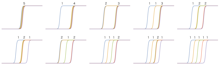
Figure 1: Amplitudes of the diagonal component of $T$ for ten different patters of five domain walls in $SU(5)$ model.

This can easily be seen as follows. First, we divide the background configuration into two parts: $SU(5)$ unbroken part and $SU(5)$ broken part as

$$\left(\begin{array}[]{c}T\\ S\end{array}\right) = \left(\begin{array}[]{c}\left(\begin{smallmatrix}\tau_{3}{\bf 1}_{3}&0\\ 0&\tau_{2}{\bf 1}_{2}\end{smallmatrix}\right)\\ \left(\begin{smallmatrix}\sigma_{3}{\bf 1}_{3}&0\\ 0&\sigma_{2}{\bf 1}_{2}\end{smallmatrix}\right)\end{array}\right)$$ (III.20)

$$= \mathbf{1}_{5}\otimes\left(\begin{array}[]{c}\frac{3\tau_{3}+2\tau_{2}}{5}\\ \frac{3\sigma_{3}+2\sigma_{2}}{5}\end{array}\right)+\left(\begin{array}[]{cc}\frac{2}{5}\mathbf{1}_{3}&\\ &-\frac{3}{5}\mathbf{1}_{2}\end{array}\right)\otimes\left(\begin{array}[]{c}\tau_{3}-\tau_{2}\\ \sigma_{3}-\sigma_{2}\end{array}\right)\,,$$ (III.27)

where we define

$$\tau_{i}\equiv v\tanh\Omega(y-{\cal Y}_{i}),\quad\sigma_{i}\equiv\bar{v}\,\mbox{sech}\,\Omega(y-{\cal Y}_{i}),\quad(i=2,3)\,.$$ (III.28)

Moreover, an infinitesimal global $SU(5)$ transformation can be parametrized as

$$U_{5}=\mathbf{1}_{5}+i\left(\begin{array}[]{cc}\alpha_{3}&\tilde{\alpha}\\ \tilde{\alpha}^{\dagger}&\alpha_{2}\end{array}\right)\,,$$ (III.31)

where $\alpha_{3}$ and $\alpha_{2}$ are $3\times 3$ and $2\times 2$ infinitesimal Hermitian matrices with ${\rm Tr}\alpha_{3}+{\rm Tr}\alpha_{2}=0$ belonging to $SU(3)\times SU(2)\times U(1)$, while $\tilde{\alpha}$ is a 3 by 2 complex matrix containing the 12 broken generators. Applying it to Eq. (III.27) we obtain

$$\delta\left(\begin{array}[]{c}T\\ S\end{array}\right)=\left(\begin{array}[]{c}\left(\begin{smallmatrix}0&i\tilde{\alpha}(\tau_{3}-\tau_{2})\\ -i\tilde{\alpha}^{\dagger}(\tau_{3}-\tau_{2})&0\end{smallmatrix}\right)\\ \left(\begin{smallmatrix}0&i\tilde{\alpha}(\sigma_{3}-\sigma_{2})\\ -i\tilde{\alpha}^{\dagger}(\sigma_{3}-\sigma_{2})&0\end{smallmatrix}\right)\end{array}\right)=\left(\begin{array}[]{cc}0&i\tilde{\alpha}\\ -i\tilde{\alpha}^{\dagger}&0\end{array}\right)\otimes\left(\begin{array}[]{c}\tau_{3}-\tau_{2}\\ \sigma_{3}-\sigma_{2}\end{array}\right)\,.$$ (III.40)

Thus the 12 zero modes in $\tilde{\alpha}$ are nothing but the NG modes. We also have $3^{2}+2^{2}-1=12$ qNG modes living in the 3 by 3 top-left and 2 by 2 bottom-right corner of $\delta Y$. Adding the translational zero mode, we again have $12+12+1=25$ zero modes in total. It is important to observe that physics such as massive spectra and the character of massless modes (NG boson or qNG boson) differ depending on different values of moduli parameters. However, the total number of massless modes (NG and qNG together) remains the same irrespective of the value of moduli parameters Eto:2008dm .

Let us verify mass spectra and wave functions of each mode by considering small fluctuations around a background configuration. We again take the 3-2 splitting background solution (it is a straightforward task to generalize the following to other cases)

$$T = \left(\begin{array}[]{cc}\tau_{3}(y)\mathbf{1}_{3}&0\\ 0&\tau_{2}(y)\mathbf{1}_{2}\end{array}\right)+\left(\begin{array}[]{cc}t_{3}(x^{\mu},y)&\tilde{t}(x^{\mu},y)\\ \tilde{t}(x^{\mu},y)^{\dagger}&t_{2}(x^{\mu},y)\end{array}\right),$$ (III.45)

$$S = \left(\begin{array}[]{cc}\sigma_{3}(y)\mathbf{1}_{3}&0\\ 0&\sigma_{2}(y)\mathbf{1}_{2}\end{array}\right)+\left(\begin{array}[]{cc}s_{3}(x^{\mu},y)&\tilde{s}(x^{\mu},y)\\ \tilde{s}(x^{\mu},y)^{\dagger}&s_{2}(x^{\mu},y)\end{array}\right),$$ (III.50)

where the first terms on the right-hand sides are the background configurations. The second terms stand for the small fluctuations where $t_{3},s_{3}$ are 3 by 3, and $t_{2},s_{2}$ are 2 by 2 Hermitian matrices, and $\tilde{t},\tilde{s}$ are 3 by 2 complex matrices. Linearized equations of motion can be cast into the following form: The diagonal parts are of the form

$$\left(-\partial_{M}\partial^{M}-V_{i}\right)\bm{t}_{i} = 0,\qquad\bm{t}_{i}\equiv\left(\begin{array}[]{c}t_{i}\\ s_{i}\end{array}\right),$$ (III.53)

with $i=3,2$. Here, $\bm{t}_{i}$ is a two vector whose components are 3 by 3 matrices for $i=3$ and 2 by 2 matrices for $i=2$. The 2 by 2 symmetric matrix Schrödinger potential $V_{i}$ acts in the 2 component vector space $\bm{t}_{i}$. The off-diagonal part has similar structure as

$$\left(-\partial_{M}\partial^{M}-\tilde{V}\right)\tilde{\bm{t}} = 0,\qquad\tilde{\bm{t}}\equiv\left(\begin{array}[]{c}\tilde{t}\\ \tilde{s}\end{array}\right),$$ (III.56)

where $\tilde{\bm{t}}$ is a two vector whose components are 3 by 2 matrices, and $\tilde{V}$ is 2 by 2 symmetric matrix again acting in the two-vector space $\tilde{\bm{t}}$. The Schrödinger potentials are given as

$$V_{i,11} = -2\lambda^{2}(v^{2}-\tau_{i}^{2}-\sigma_{i}^{2})+4\lambda^{2}\tau_{i}^{2},$$ (III.57)

$$V_{i,12} = V_{i,21}=4\lambda^{2}\tau_{i}\sigma_{i},$$ (III.58)

$$V_{i,22} = -2\lambda^{2}(v^{2}-\sigma_{i}^{2}-\tau_{i}^{2})+4\lambda^{2}\sigma_{i}^{2}+\Omega^{2},$$ (III.59)

$$\tilde{V}_{11} = \lambda^{2}(2\tau_{3}^{2}+2\tau_{3}\tau_{2}+2\tau_{2}^{2}+\sigma_{3}^{2}+\sigma_{2}^{2}-2v^{2})+\xi(\sigma_{3}-\sigma_{2})^{2},$$ (III.60)

$$\tilde{V}_{12} = \tilde{V}_{21}=\lambda^{2}(\tau_{3}+\tau_{2})(\sigma_{3}+\sigma_{2})-\xi(\tau_{3}-\tau_{2})(\sigma_{3}-\sigma_{2}),$$ (III.61)

$$\tilde{V}_{22} = \lambda^{2}(2\sigma_{3}^{2}+2\sigma_{3}\sigma_{2}+2\sigma_{2}^{2}+\tau_{3}^{2}+\tau_{2}^{2}-2v^{2})+\xi(\tau_{3}-\tau_{2})^{2}+\Omega^{2}\,.$$ (III.62)

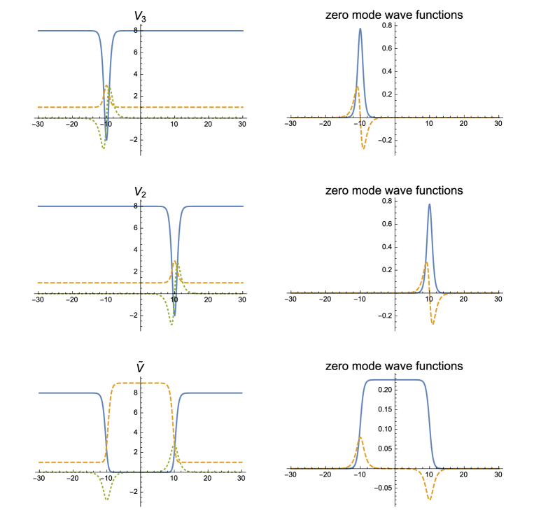
Figure 2: The Schrödinger potentials $V_{3}$, $V_{2}$ and $\tilde{V}$ ($11$ component in solid line, $22$ component in dashed line, and $12$ component in dotted line) are shown in the left panel in the top, middle and bottom row, respectively. Corresponding zero mode wave functions $\mathbbm{u}_{3}^{(0)}$, $\mathbbm{u}_{2}^{(0)}$, and $\tilde{\mathbbm{u}}^{(0)}$ (the upper component is in solid line and the lower component in the dashed line) are shown in the right panels. ${\cal Y}_{3}=-10$ and ${\cal Y}_{2}=10$ with the model parameters $v=\sqrt{2}$, $\lambda=1$, $\Omega=1$ and $\xi=1$.

Let us expand the fluctuation fields as

$$\bm{t}_{i}(x^{\mu},y) = \sum_{n}\left(\begin{array}[]{c}\eta_{i}^{(n)}(x^{\mu})\mathbbm{u}_{i;1}^{(n)}(y)\\ \eta_{i}^{(n)}(x^{\mu})\mathbbm{u}_{i;2}^{(n)}(y)\end{array}\right)=\sum_{n}\eta_{i}^{(n)}(x^{\mu})\otimes\mathbbm{u}_{i}^{(n)}(y),$$ (III.65)

$$\tilde{\bm{t}}(x^{\mu},y) = \sum_{n}\left(\begin{array}[]{c}\tilde{\eta}_{i}^{(n)}(x^{\mu})\tilde{\mathbbm{u}}_{i;1}^{(n)}(y)\\ \tilde{\eta}_{i}^{(n)}(x^{\mu})\tilde{\mathbbm{u}}_{i;2}^{(n)}(y)\end{array}\right)=\sum_{n}\tilde{\eta}^{(n)}(x^{\mu})\otimes\tilde{\mathbbm{u}}^{(n)}(y),$$ (III.68)

where the basis $\mathbbm{u}_{i}^{(n)}=(\mathbbm{u}_{i;1}^{(n)},\ \mathbbm{u}_{i;2}^{(n)})^{t}$ and $\tilde{\mathbbm{u}}^{(n)}=(\tilde{\mathbbm{u}}_{i;1}^{(n)},\ \tilde{\mathbbm{u}}_{i;2}^{(n)})^{t}$ are two vectors whose components are scalar, and the four-dimensional effective fields $\eta_{3}^{(n)}$ and $\eta_{2}^{(n)}$ are 3 by 3 and 2 by 2 Hermitian matrices while $\tilde{\eta}^{(n)}$ is 3 by 2 complex matrix. Note that the upper and lower components share the same four-dimensional effective fields $\eta_{i}^{(n)}$ and $\tilde{\eta}^{(n)}$. The mass dimensions of the fields are $[\eta]=1$ and $[\mathbbm{u}]=\frac{1}{2}$. In order to figure out the spectrum, it is convenient to define the basis by

$$\left(-\partial_{y}^{2}+V_{i}\right)\mathbbm{u}_{i}^{(n)}=m_{i,n}^{2}\mathbbm{u}_{i}^{(n)},\qquad\left(-\partial_{y}^{2}+\tilde{V}\right)\tilde{\mathbbm{u}}^{(n)}=\tilde{m}_{n}^{2}\tilde{\mathbbm{u}}^{(n)}.$$ (III.69)

The wave functions of zero modes can explicitly be obtained as

$$\mathbbm{u}_{i}^{(0)} = \frac{N_{i}}{\Omega}\,\partial_{y}\left(\begin{array}[]{c}\tau_{i}\\ \sigma_{i}\end{array}\right),$$ (III.72)

$$\tilde{\mathbbm{u}}^{(0)} = \tilde{N}\left(\begin{array}[]{c}\tau_{3}-\tau_{2}\\ \sigma_{3}-\sigma_{2}\end{array}\right),$$ (III.75)

where $N_{i}$ and $\tilde{N}$ stand for normalization constants whose mass dimensions are $[N_{i}]=[\tilde{N}]=-1$. Fig. 2 shows the wave functions. The former wave function $\mathbbm{u}^{(0)}_{i}$ is given by the $y$-derivative of the background solutions in the diagonal components. This is expected because, for example, the zero modes in the 3 by 3 top-left diagonal small matrix is given by $\tau_{3}+t_{3}=v\tanh\Omega((y-{\cal Y}_{3})\mathbf{1}_{3}+Y_{3})$ and $\sigma_{3}+s_{3}=\bar{v}\,\mbox{sech}\,\Omega((y-{\cal Y}_{3})\mathbf{1}_{3}+Y_{3})$ with $Y_{3}$ being arbitrary 3 by 3 Hermitian matrix. As usual, the zero mode wave function should be obtained by differentiating the solution in terms of the moduli parameters $Y_{3}$. Since $Y_{3}$ is a unique matrix appearing in the solution, $Y_{3}$ derivative can be replaced by $y$ derivative. That is Eq. (III.72). The zero mode of Eq. (III.75) is obtained similarly. These fluctuations correspond to the NG bosons associated with $SU(5)\to SU(3)\times SU(2)\times U(1)$ which we can see directly from infinitesimal transformation given by the off-diagonal elements of Eq. (III.40).

Defining the inner product for two-component vectors of function of $y$ as

$$(\mathbbm{u},\mathbbm{v})\equiv\int dy\,\mathbbm{u}^{t}~{}\mathbbm{v}\,,$$ (III.76)

the normalization factors are determined by the condition $\left(\mathbbm{u}_{i}^{(0)},\mathbbm{u}_{i}^{(0)}\right)=\left(\tilde{\mathbbm{u}}^{(0)},\tilde{\mathbbm{u}}^{(0)}\right)=1$. $\tilde{N}$ can be explicitly evaluated to give a function of the wall distance $L=|{\cal Y}_{2}-{\cal Y}_{3}|$ as

$$\frac{1}{\tilde{N}^{2}}=4L\left(\frac{\Omega^{2}}{\lambda^{2}}\frac{1}{\sinh L\Omega}+v^{2}\tanh\frac{L\Omega}{2}\right)-\frac{4\Omega}{\lambda^{2}}\,.$$ (III.77)

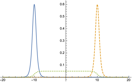
Figure 3: The profiles of kinetic terms $\rho(\bm{t}_{3}^{(0)};y)$ (solid), $\rho(\bm{t}_{2}^{(0)};y)$ (dashed) and $\rho(\tilde{\bm{t}}^{(0)};y)$ (dotted) are shown for ${\cal Y}_{3}=-10$ and ${\cal Y}_{2}=10$ with the model parameters $v=\sqrt{2}$, $\lambda=1$ and $\Omega=1$,

To understand where the effective fields are localized, let us define the profiles of kinetic terms for zero modes as

$$\rho(\bm{t}_{i}^{(0)};y)=\mathbbm{u}_{i}^{(0)t}~{}\mathbbm{u}_{i}^{(0)},\qquad\rho(\tilde{\bm{t}}^{(0)};y)=\tilde{\mathbbm{u}}^{(0)t}~{}\tilde{\mathbbm{u}}^{(0)}\,,$$ (III.78)

with the mass dimension $[\rho]=1$ (compensating the mass dimension $-1$ from a $y$ integral). As illustrated by a typical example shown in Fig. 3, the eight qNGs in $\eta_{3}^{(0)}(x^{\mu})$ are localized on the left three coincident walls while the three qNGs in $\eta_{2}^{(0)}(x^{\mu})$ are localized on the right two coincident walls. The profile of kinetic term for the translational NG mode is a linear combination $(\rho(\bm{t}^{(0)}_{3};y)+\rho(\bm{t}^{(0)}_{2};y))/2$, which has a support on both the left and right walls. Finally, $\rho(\tilde{\bm{t}}^{(0)};y)$ provides the distribution for the twelve NGs $\tilde{\eta}^{(0)}(x^{\mu})$ associated with $SU(5)\to SU(3)\times SU(2)\times U(1)$ spreading between the left and right walls. The reason why $\tilde{\eta}^{(0)}$ localizes between walls is clear. It is because the region between walls is asymptotically close to the vacuum $\left<3,2\right>$ where $SU(5)$ is partially broken. They are called the non-Abelian cloud of the non-Abelian domain wall Eto:2008dm .

The geometric Higgs mechanism
As long as the $SU(5)$ is a global symmetry, the $25$ zero modes are all physical degrees of freedom. However, once the gauge interaction is turned on, the $SU(5)$ becomes a local symmetry. Then the qNGs do remain as the physical zero modes whereas the NGs (except for the translational zero mode) will disappear from the physical spectra because they are absorbed into gauge bosons as their longitudinal components. Thus, the breaking pattern of the gauge symmetry is determined by the domain wall positions in the $y$ directions. By counting from the left-most wall, when the numbers of coincident walls is $(k_{1},k_{2},\cdots,k_{n})$ with $\sum_{i=1}^{n}{k_{i}}=5$, the gauge symmetry is broken as $SU(5)\to S[U(k_{1})\times U(k_{2})\times\cdots\times U(k_{n})]$. One should note that the Higgs mechanism occurs locally since the would-be NG modes are localized between the split walls. This is the heart of the geometric Higgs mechanism which we are going to explain in detail in the subsequent section.
 

Finally, let us make comments on massive modes. In general, it is not easy to determine the massive modes because the linearized equations of motion (III.53) and (III.56) represent a coupled system of Schrödinger-like equations. Nevertheless, some important information can be derived from the asymptotic values of the potentials

$$\lim_{y\to\pm\infty}V_{3}=\lim_{y\to\pm\infty}V_{2}=\lim_{y\to\pm\infty}\tilde{V}=\left(\begin{array}[]{cc}4\lambda^{2}v^{2}&0\\ 0&\Omega^{2}\end{array}\right).$$ (III.81)

Firstly, we see that all the off-diagonal components vanish (see dotted lines on the left panels of Fig. 2). Therefore, the upper and lower components of $\mathbbm{u}_{i}^{(n)}$ and $\tilde{\mathbbm{u}}^{(n)}$ are asymptotically decoupled and become free. They interfere only near the domain walls. Secondly, we see that there is a common mass gap between massless modes and continuum spectrum. The mass gap is given by $\min\{2\lambda v,\Omega\}$. Massive modes will be localized between the walls because they are bounded by the quasi-square well $\tilde{V}_{11}$ as is shown in the left-bottom panel (solid line) of Fig. 2.

Figure 4: Left: the Schrödinger potential $\tilde{V}_{11}$ and wave functions of the zero mode and the first excited mode in the off-diagonal component are shown for $L=10$. Right: the masses of first excited modes are plotted in red dots. The solid curve is numerical fit by $3.5/L$. The parameters are $\lambda=v=1$.

In order to get a better insight, let us further simplify the global $SU(5)$ model (III.12) and (III.13) by dropping the $S$ field. Then, the simplified model is just an extension of $\phi^{4}$ type model with the adjoint scalar $T$ only. The background wall solution is given by $T=v\tanh v\lambda(y-Y)$. Let us consider fluctuations like in Eq. (III.45) with $\tau_{i}=v\tanh v\lambda(y-{\cal Y}_{i})$ for the 3-2 splitting. The Schrödinger equations for the fluctuations are obtained by just picking up the upper components of Eqs. (III.53) and (III.56). The Schrödinger potential for the diagonal part is $V_{i,11}$ given in Eq. (III.57) with $\sigma_{i}$ being replaced by $0$. This is nothing but the Schrödinger equation for linear fluctuations around a domain wall in ordinary $\phi^{4}$ model whose spectrum is well-known: the lowest modes are massless and the first excited modes have mass $\sqrt{3}\,\lambda v$. In our reduced model, these modes are the 3 by 3 and 2 by 2 matrices in the adjoint representation of $SU(3)$ and $SU(2)$. Note that these modes are blind to whether the $SU(5)$ symmetry is global or local. Similarly, the Schrödinger potential for the off-diagonal components is given by $\tilde{V}_{11}$ in Eq. (III.61) with $\sigma_{i}\to 0$. Since the existence of zero modes for the off-diagonal components is protected by symmetry, the upper elements of (III.75) remain as massless modes localized between the domain walls. On the other hand, we need a numerical computation to obtain excited modes since the Schrödinger equation cannot be solved analytically except for two extreme limits: zero separation limit $|{\cal Y}_{3}-{\cal Y}_{2}|=0$, and infinite separation limit ${\cal Y}_{2}\to\infty$ and ${\cal Y}_{3}\to-\infty$, namely the vacuum $T={\rm diag}(v,v,v,-v,-v)$. In the former limit, $SU(5)$ symmetry is unbroken, and therefore both zero modes and excited modes form $SU(5)$ multiplets. This means that $t_{3}$, $t_{2}$ and $\tilde{t}$ are all on an equal footing, so that mass of the first excited mode in $\tilde{t}$ should be $\sqrt{3}\,\lambda v$ as that for $\phi^{4}$ kink. In the latter limit the off-diagonal components are the massless NGs. Thus, for the finite separation $L$, the mass of the first excited mode $\tilde{t}$ is a continuous function, say $\tilde{m}(L)$, of the separation $L=|{\cal Y}_{3}-{\cal Y}_{2}|$, which asymptotically behaves as $\tilde{m}\to\sqrt{3}\,\lambda v$ at $L\to 0$ and $\tilde{m}\to 0$ at $L\to\infty$. Indeed, the Schrödinger potential $\tilde{V}_{11}$ at large $L$ is almost square well whose height is $4\lambda^{2}v^{2}$ and width is $L$. Therefore, $\tilde{m}$ behaves as $1/L$ at the large $L$ limit, see Fig. 4. In short, the mass spectrum of the off-diagonal element for well separated domain walls starts from zero and is followed by the massive modes of order $1/L$.

Thus we got an understanding that the off-diagonal components have a zero mode and light massive modes of order $1/L$ in the $SU(N)$ global model. Whereas the zero mode will be eaten by the gauge fields, one might anticipate the light massive modes appearing between the domain walls. But we emphasis that this is the case where $SU(5)$ is global symmetry. As we will see in later sections, gauging $SU(5)$ will get rid of the off-diagonal zero modes and, at the same time, it increases the masses of massive modes.

IV Mass spectrum on domain walls in local $SU(N)$ model

Now, we come to main part of this work. Our aim here is to determine the physical spectrum around the background domain walls (III.5) in the gauged model (II.1). The case where all the $N$ domain walls are on top of each other has been intensively studied in Refs. Ohta ; Us1 ; Us2 , and the localization mechanism of massless $SU(N)$ gauge fields on the coincident walls is well understood. In contrast, in this work, we will focus on the case where some domain walls are separated from each other. Especially, we will clarify how the massless $SU(N)$ gauge fields acquire non-zero masses, namely the geometric Higgs mechanism.

We continue to consider the $SU(5)$ model and the $3$-$2$ split domain wall solution (III.7) with $Y={\rm diag}({\cal Y}_{3},{\cal Y}_{3},{\cal Y}_{3},{\cal Y}_{2},{\cal Y}_{2})$, for its phenomenological significance. Extension of our results to both generic number of walls and arbitrary configurations is straightforward.

IV.1 Linearized equations of motion

Let us derive linearized equations of motion for small fluctuations around the $3$-$2$ splitting background solution. The fluctuations in the scalar fields $T,S$ are given in Eqs. (III.45) and (III.50). As this background breaks $SU(5)$ gauge symmetry down to standard model (SM) group $G_{\rm SM}=SU(3)\times SU(2)\times U(1)_{Y}$, let us parametrize the surviving symmetry transformations as

$$U_{5}=\begin{pmatrix}U_{3}&0\\ 0&U_{2}\end{pmatrix}e^{i\frac{\alpha T_{Y}}{2}}\,,\qquad T_{Y}=\left(\begin{array}[]{cc}-\frac{2}{3}\mathbf{1}_{3}&0\\ 0&\mathbf{1}_{2}\end{array}\right)\,,$$ (IV.1)

where $U_{3}\in SU(3)$, $U_{2}\in SU(2)$ and $\alpha\in U(1)_{Y}$. In the following, let us employ the axial gauge in $4+1$ dimensions

$$A_{y}=0\,.$$ (IV.2)

There is a residual gauge transformation which depends only on $x^{\mu}$ coordinate. Further, let us separate diagonal and off-diagonal degrees of freedom in fluctuations of the gauge fields as

$$A_{\mu}=0+\begin{pmatrix}a_{3\mu}&b_{\mu}\\ b_{\mu}^{\dagger}&a_{2\mu}\end{pmatrix}+a_{1\mu}T_{1}\,,\qquad T_{1}=\sqrt{\frac{3}{5}}\left(\begin{array}[]{cc}\frac{1}{3}\mathbf{1}_{3}&0\\ 0&-\frac{1}{2}\mathbf{1}_{2}\end{array}\right)\,,$$ (IV.3)

where $a_{3\mu}$ is a $3\times 3$ Hermitian traceless matrix and $a_{2\mu}$ is a $2\times 2$ Hermitian traceless matrix, while $b_{\mu}$ is a $3\times 2$ complex matrix. The gauge fields $a_{3\mu}$, $a_{2\mu}$, and $a_{1\mu}$ for $SU(3)$, $SU(2)$ and $U(1)_{Y}$ transform under the SM gauge group as

$$a_{3\mu} \to U_{3}a_{3\mu}U_{3}^{\dagger}+i\partial_{\mu}U_{3}U_{3}^{\dagger}\,,$$ (IV.4)

$$a_{2\mu} \to U_{2}a_{2\mu}U_{2}^{\dagger}+i\partial_{\mu}U_{2}U_{2}^{\dagger}\,,$$ (IV.5)

$$a_{1\mu} \to a_{1\mu}+\sqrt{\frac{5}{3}}\partial_{\mu}\alpha.$$ (IV.6)

On the other hand, the $b_{\mu}$ field transforms as

$$b_{\mu}\to U_{3}b_{\mu}U_{2}^{\dagger}e^{-\frac{5i\alpha}{6}}\,.$$ (IV.7)

To investigate the spectrum, we need to write down the linearized equations of motion for each component of (III.45), (III.50) and (IV.3). Plugging these into equations of motion (II.7) – (II.9), we end up with

$$\partial_{M}\Bigl{(}\sigma_{\alpha}^{2}f_{\alpha}^{MN}\Bigr{)} =0\,,$$ (IV.8)

$$\left(-\partial_{M}\partial^{M}-V_{i}\right)\bm{t}_{i} =0\,,$$ (IV.9)

$$a\partial_{M}\left(\sigma_{+}^{2}C^{MN}\right) =-\frac{i}{\tilde{N}}\tilde{\mathbbm{u}}^{(0)t}\left(\overleftrightarrow{\partial}^{N}\tilde{\bm{t}}-\frac{i}{\tilde{N}}b^{N}\otimes\tilde{\mathbbm{u}}^{(0)}\right)\,,$$ (IV.10)

$$\left(-\partial_{M}\partial^{M}-\tilde{V}\right)\tilde{\bm{t}} =-\frac{i}{\tilde{N}}\left(\partial_{M}b^{M}\right)\tilde{\mathbbm{u}}^{(0)}-\frac{2i}{\tilde{N}}b^{M}\otimes\partial_{M}\tilde{\mathbbm{u}}^{(0)}\,,$$ (IV.11)

where no sum is taken for $\alpha=1,2,3$ and $i=3,2$ in Eqs. (IV.8)–(IV.9). The linearized field strength is defined as usual by $f_{\alpha}^{MN}=\partial^{M}a_{\alpha}^{N}-\partial^{N}a_{\alpha}^{M}$, and $\sigma_{i}$ ($i=2,3)$ is defined in (III.28). In addition, we have introduced

$$\sigma_{1}=\sqrt{\frac{2\sigma_{3}^{2}+3\sigma_{2}^{2}}{5}}\,,\quad\sigma_{+}=\sqrt{\sigma_{3}^{2}+\sigma_{2}^{2}}\,,\quad C^{MN}=\partial^{M}b^{N}-\partial^{N}b^{M}\,,$$ (IV.12)

and $\tilde{\mathbbm{u}}^{(0)}$ is given in Eq. (III.75).

IV.2 Diagonal components

First, we find that the fluctuations $a_{\alpha}^{\mu}$ ($\mu=0,1,2,3$, $\alpha=1,2,3$) and $\bm{t}_{i}$ ($i=3,2$) in the diagonal parts are decoupled from the other fields. Especially, Eq. (IV.9) for $\bm{t}_{i}$ is exactly the same as Eq. (III.53). Therefore, we have $9$ and $4$ zero modes in $\bm{t}_{3}$ and $\bm{t}_{2}$ whose wave functions have been determined as $\mathbbm{u}_{3}^{(0)}$ and $\mathbbm{u}_{2}^{(0)}$ given in Eq. (III.72).

Let us next investigate spectrum for the unbroken parts of the gauge fields given in Eq. (IV.8). The $N=y$ component in the axial gauge ($b_{y}=0$) is

$$\sigma_{\alpha}^{2}\partial_{y}\partial_{\mu}a_{\alpha}^{\mu}=0\,,\qquad\text{(no sum for $\alpha$)},$$ (IV.13)

and the $N=\nu$ component is

$$\sigma_{\alpha}^{2}\partial_{\mu}f_{\alpha}^{\mu\nu}+\partial_{y}(\sigma_{\alpha}^{2}\partial^{y}a_{\alpha}^{\nu})=0\,,\qquad\text{(no sum for $\alpha$)}.$$ (IV.14)

We can decompose the gauge field into divergence-free and divergence components as

$$a_{\alpha}^{\mu}=a_{\alpha,{\rm df}}^{\mu}+a_{\alpha,{\rm d}}^{\mu}\,\quad a_{\alpha,{\rm df}}^{\mu}=({\cal P}_{\rm df})^{\mu}{}_{\nu}a_{\alpha}^{\nu}\,,\quad a_{\alpha,{\rm d}}^{\mu}=({\cal P}_{\rm d})^{\mu}{}_{\nu}a_{\alpha}^{\nu}\,,$$ (IV.15)

where we introduced the projection operators

$$({\cal P}_{\rm d})^{\mu}{}_{\nu}=\frac{\partial^{\mu}\partial_{\nu}}{\partial^{2}}\,,\qquad({\cal P}_{\rm df})^{\mu}{}_{\nu}=\delta^{\mu}_{\nu}-\frac{\partial^{\mu}\partial_{\nu}}{\partial^{2}}\,,$$ (IV.16)

with the four-dimensional Laplacian $\partial^{2}=\partial_{\mu}\partial^{\mu}$. They satisfy the following identities

$$\partial_{\mu}a_{\alpha,{\rm df}}^{\mu}=0\,,\quad a_{\alpha,{\rm d}}^{\mu}=\frac{1}{\partial^{2}}\partial^{\mu}F_{\alpha},\quad F_{\alpha}=\partial_{\nu}a_{\alpha}^{\nu}\,.$$ (IV.17)

The $N=y$ equation tells us that $\partial_{y}F_{\alpha}=0$, so that we have $F_{\alpha}=F_{\alpha}(x^{\mu})$ which can be gauged away by using $SU(3)\times SU(2)\times U(1)_{Y}$ gauge transformation. Then the $N=\nu$ component reads

$$\sigma_{\alpha}^{2}\left(\partial^{2}-\partial_{y}^{2}\right)a_{\alpha,{\rm df}}^{\nu}-(\partial_{y}\sigma_{\alpha}^{2})\partial_{y}a_{\alpha,{\rm df}}^{\nu}=0\,,\qquad\text{(no sum for $\alpha$)}.$$ (IV.18)

To find the spectrum, let us expand the divergence-free component as

$$a_{\alpha,{\rm df}}^{\nu}=\sum_{n}w_{\alpha\nu}^{(n)}(x^{\mu})f_{a,\alpha}^{(n)}(y)\equiv\sum_{n}w_{\alpha\nu}^{(n)}(x^{\mu})\frac{v_{\alpha}^{(n)}(y)}{\sigma_{\alpha}(y)},$$ (IV.19)

where $w_{\alpha\nu}^{(n)}(x^{\mu})$ is the four-dimensional gauge fields (matrix) and $v_{\alpha}^{(n)}(y)/\sigma_{\alpha}(y)$ is its wave function (one component). The mass dimensions are given by $[w_{\alpha\mu}^{(n)}]=1$ and $[v_{\alpha}^{(n)}]=\frac{3}{2}$. The basis of expansion is defined by the Schrödinger equation

$$\left(-\partial_{y}^{2}+V_{\alpha}\right)v_{\alpha}^{(n)}=\mu_{\alpha,n}^{2}v_{\alpha}^{(n)},\quad V_{\alpha}\equiv\frac{1}{\sigma_{\alpha}}\partial_{y}^{2}\sigma_{\alpha}=\Omega^{2}\left(1-2\,\mbox{sech}^{2}\Omega(y-{\cal Y}_{\alpha})\right),$$ (IV.20)

where no sum is taken for $\alpha$.

This Schrödinger-type problem can be cast into the following form

$$H_{\alpha}v_{\alpha}^{(n)}=\mu_{\alpha,n}^{2}v_{\alpha}^{(n)}\,,\quad H_{\alpha}=Q_{\alpha}^{\dagger}Q_{\alpha}\,,$$ (IV.21)

where we define

$$Q_{\alpha}=\partial_{y}-\partial_{y}\log\sigma_{\alpha}\,,\quad Q_{\alpha}^{\dagger}=-\partial_{y}-\partial_{y}\log\sigma_{\alpha}\,.$$ (IV.22)

There are two benefits for this expression. First, the Hamiltonian is manifestly positive definite, so that we can be sure that no tachyonic modes exist in the spectrum. Second, the zero mode can be easily found by solving $Qv_{\alpha}^{(0)}=0$, which gives

$$v_{\alpha}^{(0)}(y)={\cal N}_{\alpha}\,\sigma_{\alpha}(y),$$ (IV.23)

where ${\cal N}_{\alpha}$ stands for normalization constant of the mass dimension $[{\cal N}_{\alpha}]=0$. The normalization factor ${\cal N}_{\alpha}$ is fixed as ${\cal N}_{\alpha}=1$ to have properly normalized field strength $w_{\alpha}^{(0)\mu\nu}\equiv\partial^{\mu}w_{\alpha}^{(0)\nu}-\partial^{\nu}w_{\alpha}^{(0)\mu}+i\bigl{[}w_{\alpha}^{(0)\mu},w_{\alpha}^{(0)\nu}\bigr{]}$. Note that the zero mode wave functions are flat ${\cal N}_{\alpha}v_{\alpha}^{(0)}/\sigma_{\alpha}=1$, nevertheless, the massless effective gauge fields are localized on the walls thanks to the Ohta-Sakai gauge kinetic function (II.6). The profile of kinetic terms for the zero mode $w_{\alpha}^{(0)\mu}$ can be read as

$$\rho(w_{\alpha\mu}^{(0)};y)=a\sigma_{\alpha}^{2}\times\left(\frac{v_{\alpha}^{(0)}}{\sigma_{\alpha}}\right)^{2}=a(v_{\alpha}^{(0)})^{2}=a\sigma_{\alpha}^{2}\,,\qquad\text{(no sum for $\alpha$)},$$ (IV.24)

where the factor $a\sigma_{\alpha}^{2}$ reflects the gauge kinetic function (II.6). The mass dimension is $[\rho(w_{\alpha\mu}^{(0)};y)]=1$. Fig. 5 shows a typical profiles of the massless gauge fields. It clearly demonstrates that $SU(3)$ gauge fields localize on the left three coincident walls and $SU(2)$ gauge fields are trapped by the right two coincident walls. $U(1)_{Y}$ gauge fields have supports both on left and right walls.

Figure 5: The profiles of kinetic terms for $\rho(w_{3\mu}^{(0)};y)$ (solid), $\rho(w_{2\mu}^{(0)};y)$ (dashed) and $\rho(w_{1\mu}^{(0)};y)$ (dotted) are shown for ${\cal Y}_{3}=-10$ and ${\cal Y}_{2}=10$ with the model parameters $v=\sqrt{2}$, $\lambda=1$ and $\Omega=1$,

In general, the Schrödinger equation with the Hamiltonian

$$H=-\partial_{y}^{2}-\frac{c}{\cosh^{2}(y)}$$ (IV.25)

has a finite number of discrete boundstates. Their energies are given by the textbook formula

$$E_{n}=-\left(\sqrt{c+\frac{1}{4}}-\frac{1}{2}-n\right)^{2}\,,$$ (IV.26)

where $n$ takes nonnegative integer values starting from 0 up to the number, for which the expression in the parenthesis is still positive. Given this fact, it is easy to see that for the potential (IV.20) there is only the zero mode as a bound state. No other massive discrete bound states exist, while the mass gap between the zero mode and the continuum modes is $\Omega$ which is of order $M_{5}$.

The effective gauge coupling constants for the effective $SU(3)\times SU(2)\times U(1)_{Y}$ gauge group can be read as follows. Let us first decompose the gauge kinetic term (II.5) with the fluctuations $a_{i\mu}$ and $b_{\mu}=0$ in Eq. (IV.3),

$$\mathrm{Tr}\left[S^{2}G_{MN}G^{MN}\right]=\sigma_{3}^{2}\mathrm{Tr}\left[f_{3\mu\nu}f_{3}^{\mu\nu}\right]+\sigma_{2}^{2}\mathrm{Tr}\left[f_{2\mu\nu}f_{2}^{\mu\nu}\right]+\left(\frac{\sigma_{3}^{2}}{5}+\frac{3\sigma_{2}^{2}}{10}\right)f_{1\mu\nu}f_{1}^{\mu\nu}\,.$$ (IV.27)

Integrating this over $y$, we find the effective gauge couplings as

$$-\frac{1}{2g_{3}^{2}}\mathrm{Tr}\left[f_{3\mu\nu}f_{3}^{\mu\nu}\right]-\frac{1}{2g_{2}^{2}}\mathrm{Tr}\left[f_{2\mu\nu}f_{2}^{\mu\nu}\right]-\frac{1}{4g_{1}^{2}}f_{1\mu\nu}f_{1}^{\mu\nu}\,,$$ (IV.28)

with

$$\frac{1}{g_{3}^{2}}=\frac{1}{g_{2}^{2}}=\frac{1}{g_{1}^{2}}=\frac{4a\bar{v}^{2}}{\Omega}\equiv\frac{1}{g_{5}^{2}}\,.$$ (IV.29)

These are the dimensionless gauge coupling constants in $3+1$ dimensions. We see that the effective gauge couplings $g_{2}$ and $g_{3}$ are given by parameters of the model and that they are equal to each other. the $U(1)_{Y}$ coupling $e_{Y}$ is given by $e_{Y}=-\sqrt{\frac{3}{20}}g_{1}$, and is related to $g_{2}$ and $g_{3}$ as

$$\frac{1}{4e_{Y}^{2}}=\frac{2}{3g_{3}^{2}}+\frac{1}{g_{2}^{2}}=\frac{20a\bar{v}^{2}}{3\Omega}\,.$$ (IV.30)

These relations are identical to the standard $SU(5)$ GUT scenario. Hence the prediction of Weinberg angle at the GUT scale is also the same as the standard $SU(5)$ GUT: $\theta_{W}=\arctan(2e_{Y}/g_{2})$ is given as $\tan^{2}\theta_{W}=3/5$. This purely group-theoretical result arises because of the identical profile of position dependent gauge couplings for these gauge groups in our simple model. However, we can obtain different profiles for different gauge coupling function and a deviation from the standard $SU(5)$ GUT, if we consider models with more complex structure.

IV.3 The geometric Higgs mechanism

Let us next investigate the off-diagonal parts in Eqs. (IV.10) and (IV.11). These are coupled equations for the fluctuations $\tilde{\bm{t}}$ and $b^{M}$. As we have shown in Eq. (III.75), there is a zero mode $\tilde{\eta}^{(0)}(x^{\mu})\otimes\tilde{\mathbbm{u}}^{(0)}(y)$ in $\tilde{\bm{t}}$ before coupling to the $SU(5)$ gauge field. We are going to show that this zero mode disappears from the physical spectrum once the gauge interaction is turned on. This is a manifestation of the geometric Higgs mechanism. We continue to use the axial gauge $b_{y}=0$.

Let us separate the zero mode and define fields $\bar{\bm{t}}$ containing only massive modes as

$$\bar{\bm{t}}(x^{\mu},y)=\tilde{\bm{t}}(x^{\mu},y)-\tilde{\eta}^{(0)}(x^{\mu})\otimes\tilde{\mathbbm{u}}^{(0)}(y),$$ (IV.31)

where we have defined a $3$ by $2$ matrix

$$\tilde{\eta}^{(0)}(x^{\mu})=\left(\tilde{\mathbbm{u}}^{(0)}(y),\tilde{\bm{t}}(x^{\mu},y)\right)\,.$$ (IV.32)

Note that the inner product should be taken by means of Eq. (III.76), and remember that the four-dimensional fields $\tilde{\eta}^{(0)}(x^{\mu})$ is 3 by 2 matrix. Thus, $\bar{\bm{t}}$ includes only massive modes orthogonal to $\tilde{\mathbbm{u}}^{(0)}$. Let us rewrite Eqs. (IV.10) and (IV.11) by using $\bar{\bm{t}}$. The $N=\nu$ and $N=y$ components of (IV.10) are of the form

$$a\sigma_{+}^{2}\partial_{\mu}\tilde{C}^{\mu\nu}+a\partial_{y}\left(\sigma_{+}^{2}\partial^{y}\tilde{b}^{\nu}\right) = -\frac{i}{\tilde{N}}\tilde{\mathbbm{u}}^{(0)t}\,\partial^{\nu}\bar{\bm{t}}-\frac{\tilde{\mathbbm{u}}^{(0)t}\,\tilde{\mathbbm{u}}^{(0)}}{\tilde{N}^{2}}\tilde{b}^{\nu}\,,$$ (IV.33)

$$a\sigma_{+}^{2}\partial^{y}\partial_{\mu}\tilde{b}^{\mu} = \frac{i}{\tilde{N}}\tilde{\mathbbm{u}}^{(0)t}\,\overleftrightarrow{\partial^{y}}\bar{\bm{t}}\,,$$ (IV.34)

where we have defined

$$\tilde{b}^{\nu}(x^{\mu},y) = b^{\nu}(x^{\mu},y)+i\tilde{N}\partial^{\nu}\tilde{\eta}^{(0)}(x^{\mu})\,,$$ (IV.35)

$$\tilde{C}^{\mu\nu} = \partial^{\mu}\tilde{b}^{\nu}-\partial^{\nu}\tilde{b}^{\mu}\,.$$ (IV.36)

Eq. (IV.11) is also rewritten as

$$-\left(\partial^{2}+\partial_{y}^{2}-\tilde{V}\right)\bar{\bm{t}}=-\frac{i}{\tilde{N}}\left(\partial_{\mu}\tilde{b}^{\mu}\right)\otimes\tilde{\mathbbm{u}}^{(0)}\,.$$ (IV.37)

Now, we are left with Eqs. (IV.33), (IV.34) and (IV.37), and we should note that the off-diagonal scalar zero mode $\tilde{\eta}^{(0)}(x^{\mu})$ does not appear alone but is hidden in $\tilde{b}^{\nu}$. This is nothing but what happens for the standard Higgs mechanism: a massless vector field eats a scalar NG mode and acquires a mass. Indeed, one realizes that Eq. (IV.31) and (IV.35) are nothing but the residual gauge transformation $U_{5}=U_{5}(x^{\mu})\in SU(5)$ in the axial gauge $A_{y}=0$. We perform the same infinitesimal $SU(5)$ transformation as Eq. (III.40). The only difference here is that the transformation is the gauge transformation. Transforming $T$ and $S$ given in Eqs. (III.45) and (III.50) by $U_{5}$ given in Eq. (III.31) with a $3$ by $2$ matrix $\tilde{\alpha}(x^{\mu})$ of local transformation parameter, we find

$$\tilde{\bm{t}}(y,x^{\mu})\to\tilde{\bm{t}}^{\prime}(y,x^{\mu})=\tilde{\bm{t}}(y,x^{\mu})-\frac{i}{\tilde{N}}\tilde{\alpha}(x^{\mu})\otimes\tilde{\mathbbm{u}}^{(0)}(y).$$ (IV.38)

Similarly, the same infinitesimal gauge transformation of the gauge field given in Eq. (IV.3) gives

$$b_{\mu}(y,x^{\mu})\to b^{\prime}_{\mu}(y,x^{\mu})=b_{\mu}(y,x^{\mu})-\partial_{\mu}\tilde{\alpha}(x^{\mu}).$$ (IV.39)

It is easy to see that gauge transformed $\tilde{\bm{t}}^{\prime}$ in Eq. (IV.38) and $b_{\mu}^{\prime}$ in Eq. (IV.39) can be identified as $\bar{\bm{t}}$ in Eq. (IV.31) and $\tilde{b}_{\mu}$ in Eq. (IV.35), by choosing the gauge transformation parameter as $\tilde{\alpha}(x^{\mu})=-i\tilde{N}\tilde{\eta}^{(0)}(x^{\mu})$. We call this choice of gauge as the unitary gauge for the geometric Higgs mechanism.

Note also that Eq. (IV.34) is redundant because it can be derived by a combination of Eq. (IV.33) (after operating $\partial_{\nu}$) and Eq. (IV.37) (after multiplying $\tilde{\mathbbm{u}}^{(0)t}$ from left). Therefore, the spectrum is determined by Eqs. (IV.33) and (IV.37).

Let us decompose Eqs. (IV.33) and (IV.37) into divergence and divergence-free parts by applying the projection operators given in Eq. (IV.16) as

$$\tilde{b}^{\mu}=\tilde{b}_{\rm d}^{\mu}+\tilde{b}_{\rm df}^{\mu}\,,\qquad\tilde{b}_{\rm d}^{\mu}\equiv({\cal P}_{\rm d})^{\mu}{}_{\nu}\tilde{b}^{\nu}\,,\qquad\tilde{b}_{\rm df}^{\mu}\equiv({\cal P}_{\rm df})^{\mu}{}_{\nu}\tilde{b}^{\nu}\,,$$ (IV.40)

with $\partial_{\mu}\tilde{b}_{\rm df}^{\mu}=0$ due to $({\cal P}_{\rm df})^{\mu}{}_{\nu}\partial^{\nu}=0$. Now, Eqs. (IV.33) and (IV.37) are written as

$$a\sigma_{+}^{2}\partial^{2}\tilde{b}_{\rm df}^{\nu}+a\partial_{y}\left(\sigma_{+}^{2}\partial^{y}\tilde{b}_{\rm df}^{\nu}\right) = -\frac{\tilde{\mathbbm{u}}^{(0)t}\,\tilde{\mathbbm{u}}^{(0)}}{\tilde{N}^{2}}\tilde{b}_{\rm df}^{\nu}\,,$$ (IV.41)

$$a\partial_{y}\left(\sigma_{+}^{2}\partial^{y}\tilde{b}_{\rm d}^{\mu}\right) = -\frac{i}{\tilde{N}}\tilde{\mathbbm{u}}^{(0)t}\left(\partial^{\mu}\bar{\bm{t}}-\frac{i}{\tilde{N}}\tilde{b}_{\rm d}^{\mu}\otimes\tilde{\mathbbm{u}}^{(0)}\right)\,,$$ (IV.42)

$$-\left(\partial_{y}^{2}-\tilde{V}\right)\bar{\bm{t}} = \partial_{\mu}\left(\partial^{\mu}\bar{\bm{t}}-\frac{i}{\tilde{N}}\tilde{b}_{\rm d}^{\mu}\otimes\tilde{\mathbbm{u}}^{(0)}\right)\,.$$ (IV.43)

Benefit of this decomposition is that the divergence-free part $\tilde{b}_{\rm df}^{\mu}$ is decoupled from the other fields. For the time being, we will concentrate on Eq. (IV.41) and find the spectrum of $\tilde{b}_{\rm df}^{\mu}$. To this end, let us expand

$$\tilde{b}_{\rm df}^{\mu}(x^{\nu},y)=\sum_{n}\beta^{(n)\mu}(x^{\nu})\frac{\gamma^{(n)}(y)}{\sigma_{+}(y)}\,.$$ (IV.44)

where $\beta_{\mu}^{(n)}$ is 3 by 2 complex matrix satisfying the divergence-free condition $\partial^{\mu}\beta_{\mu}^{(n)}=0$. The mass dimensions are $[\beta_{\mu}^{(n)}]=1$ and $[\gamma^{(n)}]=\frac{3}{2}$. Plugging this into Eq. (IV.41), we are lead to

$$\left(\partial^{2}+k_{n}^{2}\right)\beta^{(n)\nu}=0\,,$$ (IV.45)

$$\left(-\partial_{y}^{2}+{\cal V}(y)\right)\gamma^{(n)}=\tilde{\mu}_{n}^{2}\gamma^{(n)}\,,$$ (IV.46)

$${\cal V}(y)=\frac{1}{\sigma_{+}}\partial_{y}^{2}\sigma_{+}+\frac{1}{\tilde{N}^{2}}\frac{\tilde{\mathbbm{u}}^{(0)t}\,\tilde{\mathbbm{u}}^{(0)}}{a\sigma_{+}^{2}}\,.$$ (IV.47)

Note that the Schrödinger equation can be written in the following form

$$\tilde{H}\gamma^{(n)}=\tilde{\mu}_{n}^{2}\gamma^{(n)}\,,$$ (IV.48)

with the Hamiltonian

$$\tilde{H}=\tilde{Q}^{\dagger}\tilde{Q}+\frac{1}{\tilde{N}^{2}}\frac{\tilde{\mathbbm{u}}^{(0)t}\,\tilde{\mathbbm{u}}^{(0)}}{a\sigma_{+}^{2}}\,,$$ (IV.49)

where we have defined differential operators

$$\tilde{Q}=\partial_{y}-\partial_{y}\log\sigma_{+},\qquad\tilde{Q}^{\dagger}=-\partial_{y}-\partial_{y}\log\sigma_{+}.$$ (IV.50)

Note that the second term of the Hamiltonian $\tilde{H}$ is positive everywhere if ${\cal Y}_{3}\neq{\cal Y}_{2}$. Only when ${\cal Y}_{3}={\cal Y}_{2}$ it vanishes and Hamiltonian becomes $\tilde{H}=\tilde{Q}^{\dagger}\tilde{Q}$. In this coincident wall limit, there exists a zero mode which satisfies $\tilde{Q}\gamma^{(0)}=0$. It is easily solved as

$$\gamma^{(0)}=N_{+}\sigma_{+}\,,\qquad N_{+}=1\,.$$ (IV.51)

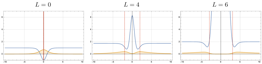
Figure 6: The Schrödinger potential ${\cal V}$ (blue solid) and the wave function (orange solid filling) of the lightest mode $\gamma^{(0)}$ for $L=0$ , $L=4$ and $L=6$ are shown. The model parameters are chosen as $a=1$, $v=\sqrt{2}$, $\lambda=1$ and $\Omega=1$. The red dashed lines show positions of the domain walls.

The zero mode (IV.51) should exist because $SU(5)$ gauge symmetry is fully unbroken in the coincident wall limit where not only the diagonal components but also off-diagonal components of the gauge fields are massless. Since $\tilde{Q}^{\dagger}\tilde{Q}$ is positive definite, the zero eigenvalue is minimum among all other eigenvalues. When the 3-2 splitting occurs, no matter how small the separation is, the second term of $H$ has a positive contribution to $\tilde{Q}^{\dagger}\tilde{Q}$. Therefore, the minimum of the spectrum for Eq. (IV.48) is positive whenever the walls split. Thus, we conclude $\tilde{\mu}_{n}^{2}>0$ for the 3-2 splitting background. Let us write the lowest mass field as $\beta_{\mu}=n_{\mu}e^{ik^{\nu}x_{\nu}}$ with $k^{2}=\tilde{\mu}_{0}^{2}$. The transverse condition $\partial_{\mu}\beta^{\mu}=0$ implies $k_{\mu}n^{\mu}=0$. Since $k^{2}=\tilde{\mu}_{0}^{2}>0$, there are three orthonormal vectors $n_{a}^{\mu}$ ($a=1,2,3)$. Namely, the vector field $\tilde{b}^{\mu}_{\rm df}$ orthonormal to $k^{\mu}$ is massive with three physical degrees of freedom (2 transverse and 1 longitudinal). This is evidently due to the geometric Higgs mechanism.

Let us obtain the first massive mode. The Schrödinger potential ${\cal V}$ for $L=|{\cal Y}_{2}-{\cal Y}_{3}|=0,4,6$ cases are shown in Fig. 6. In the limit with $\Omega L\ll 1$ where the separation is very small, the second term of ${\cal V}$ can be treated as a perturbation to $L=0$ case. Since there exists a localized zero mode $\gamma^{(0)}=\sigma_{+}$ in the $L=0$ limit, we expect the bound state remains as massive state as long as $\Omega L\ll 1$. The mass shift is estimated as

$$\tilde{\mu}_{0}(L)^{2} = \frac{\bigg{<}\gamma^{(0)}\bigg{|}\frac{1}{\tilde{N}^{2}}\frac{\tilde{\mathbbm{u}}^{(0)t}\tilde{\mathbbm{u}}^{(0)}}{a\sigma_{+}^{2}}\bigg{|}\gamma^{(0)}\bigg{>}}{\big{<}\gamma^{(0)}\big{|}\gamma^{(0)}\big{>}}=\frac{1}{a\tilde{N}^{2}\big{<}\gamma^{(0)}\big{|}\gamma^{(0)}\big{>}}$$ (IV.52)

$$= \frac{\Omega}{4a\bar{v}^{2}}\left[4L\left(\frac{\Omega^{2}}{\lambda^{2}}\frac{1}{\sinh L\Omega}+v^{2}\tanh\frac{L\Omega}{2}\right)-\frac{4\Omega}{\lambda^{2}}\right]$$

$$\simeq \frac{2}{3}g_{5}^{2}\,\Omega\left(2v^{2}+\bar{v}^{2}\right)L^{2}\,,\qquad(\Omega L\ll 1)\,,$$ (IV.53)

where we have used $\frac{1}{g_{5}^{2}}=\frac{4a\bar{v}^{2}}{\Omega}$ as is obtained in Eq. (IV.29), $\big{<}\gamma^{(0)}\big{|}\gamma^{(0)}\big{>}=\frac{4\bar{v}^{2}}{\Omega}$, and $\tilde{N}$ is given in Eq. (III.77). This approximation is compared with numerically obtained masses in Fig. 7. They nicely match for $\Omega L\ll 1$.

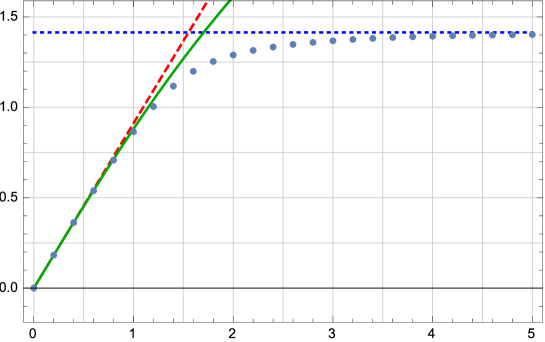
Figure 7: The mass $\tilde{\mu}_{0}(L)$ of the lowest discrete massive state of the off-diagonal divergence-free vector field $\tilde{b}_{\rm df}^{\mu}$ as a function of $L=|{\cal Y}_{3}-{\cal Y}_{2}|$. The dots are numerically obtained, the green-solid curve is analytic approximation given in Eq. (IV.52), and the red-dashed line is a linear approximation with $k_{0}(0)=0$ and $k_{0}(0.1)=0.182252$. The model parameters are chosen as $a=1$, $v=\sqrt{2}$, $\lambda=1$ and $\Omega=1$. The blue-dotted line shows the mass gap $\sqrt{\Omega^{2}+1/a}=\sqrt{2}$.

This behavior resembles the standard Higgs mechanism that mass of the vector boson is a product of a gauge coupling and a scalar vacuum expectation value (VEV). The mass formula (IV.53) tells that the effective VEV is

$$v_{\rm eff}=\sqrt{\frac{2}{3}\,\Omega\left(2v^{2}+\bar{v}^{2}\right)}\,L\,,$$ (IV.54)

so that the mass is given by $\tilde{\mu}_{0}(L)^{2}=g_{5}v_{\rm eff}$.

Note that peculiar phenomena in the geometric Higgs mechanism in our specific model appear in the opposite limit $L\Omega\gg 1$. Indeed, as $L$ being increased, the bottom of the well is lifted, and high potential barrier appears at the center of the domain walls. Height of the potential is exponentially large as

$${\cal V}(0)=\frac{\cosh\Omega L-1}{a}+2\Omega^{2}-3\Omega^{2}\mbox{sech}^{2}\frac{L\Omega}{2}\quad\to\quad\frac{e^{L\Omega}}{2a}\qquad\text{as}\quad L\to\infty\,.$$ (IV.55)

Therefore, for large separations $\Omega L\gg 1$, as shown in Fig. 6, the massive vector bosons are located not between but on the domain walls, and their masses asymptotically approach to threshold mass $\sqrt{\Omega^{2}+1/a}$ which can be read from ${\cal V}(\pm\infty)=\Omega^{2}+\frac{1-\mbox{sech}\Omega L}{a}\sim\Omega^{2}+1/a$. Thus, when the wall separation is large, the mass of vector boson becomes universal which is about $\sqrt{\Omega^{2}+1/a}$ irrespective of $L$, which is of order $M_{5}$.

Finally, we have to solve the coupled equations (IV.42) and (IV.43) for the divergence part $\tilde{b}_{\rm d}^{\mu}$ and $\bar{\bm{t}}$. Let us introduce

$$\partial^{\mu}B \equiv \sigma_{+}\,\partial^{\mu}\frac{\partial^{\nu}}{\partial^{2}}\tilde{b}_{\nu}=\sigma_{+}\tilde{b}_{\rm d}^{\mu}\,,$$ (IV.56)

$$\bar{\bm{t}}^{\prime} \equiv \bar{\bm{t}}-\frac{i}{\tilde{N}}\frac{B}{\sigma_{+}}\otimes\tilde{\mathbbm{u}}^{(0)}\,.$$ (IV.57)

There is redundancy that any function of $y$ can be added to $B$. Now Eqs. (IV.42) and (IV.43) are rewritten as

$$\partial^{\mu}\left[a\sigma_{+}\tilde{Q}^{\dagger}\tilde{Q}B+\frac{i}{\tilde{N}}\tilde{\mathbbm{u}}^{(0)t}\,\bar{\bm{t}}^{\prime}\right]=0\,,$$ (IV.58)

$$\left(-\partial_{y}^{2}+\tilde{V}\right)\left(\bar{\bm{t}}^{\prime}+\frac{i}{\tilde{N}}\frac{B}{\sigma_{+}}\otimes\tilde{\mathbbm{u}}^{(0)}\right)=\partial^{2}\bar{\bm{t}}^{\prime}\,,$$ (IV.59)

where $\tilde{Q}$ and $\tilde{Q}^{\dagger}$ are defined in Eq. (IV.50). The former equation can formally be solved as

$$B=\left(\tilde{Q}^{\dagger}\tilde{Q}\right)^{-1}\left(\frac{-i}{a\tilde{N}\sigma_{+}}\tilde{\mathbbm{u}}^{(0)t}\,\bar{\bm{t}}^{\prime}+\Lambda(y)\right)\,,$$ (IV.60)

where $\Lambda(y)$ is an arbitrary function of $y$ which we may set 0 by absorbing in the redundancy of $B$. Plugging this into Eq. (IV.59), one can eliminate $B$ and we are left with

$$\partial^{2}\bar{\bm{t}}^{\prime}=\left(-\partial_{y}^{2}+\tilde{V}\right)\left\{\bar{\bm{t}}^{\prime}+\frac{i}{\tilde{N}}\frac{1}{\sigma_{+}}\left[\left(\tilde{Q}^{\dagger}\tilde{Q}\right)^{-1}\left(\frac{-i}{a\tilde{N}\sigma_{+}}\tilde{\mathbbm{u}}^{(0)t}\,\bar{\bm{t}}^{\prime}\right)\right]\otimes\tilde{\mathbbm{u}}^{(0)}\right\}\,.$$ (IV.61)

This formally determines the mass spectrum for $\bar{\bm{t}}^{\prime}$ although it is not easily solved analytically. Once we do this, $B$ is determined from Eq. (IV.60). Thus, as usual, the divergence part $\tilde{b}_{\rm d}^{\mu}$ does not have independent physical degrees of freedom, so that Eq. (IV.42) should be regarded as the constraint reducing the four polarization degrees of freedom in a massive vector field by one.

Instead of trying to solve Eq. (IV.61), let us understand the spectrum defined by seeing Eq. (IV.61) from a different viewpoint. Let us first recall that the second term on the right-hand side of Eq. (IV.43) or (IV.61) reflects the fact that we gauged $SU(5)$ symmetry of the corresponding mode equation (III.56) in the scalar model considered in Sec. III.2. As was mentioned at the end of Sec. III.2, when $SU(5)$ is global symmetry, the four-dimensional effective fields in $\tilde{\bm{t}}$ (or $\bar{\bm{t}}$) are all massless NGs at the infinite wall separation, and they, except for the genuine NGs, are lifted and obtain non-zero mass of order the inverse separation $\sim 1/L$ when the walls are separated by $L$. This is similar to the standard compactification of the fifth direction to $S^{1}/Z_{2}$ with radius $R$. In our theory, the extra dimension is infinitely large and our compactification is a posteriori done by the domain walls with the compactification size $L$. On the other hand, in the $S^{1}/Z_{2}$ model the extra dimension is compact a priori. For simplicity, let us compare the simplest models, the $U(1)$ Goldstone (global) model and Abelian-Higgs (gauge) model in five dimensions compactified by $S^{1}/Z_{2}$ orbifolding,

$${\cal L}_{\rm global} = |D_{M}\phi|^{2}-\frac{\lambda^{2}}{4}\left(|\phi|^{2}-v^{2}\right)^{2}\,,$$ (IV.62)

$${\cal L}_{\rm local} = -\frac{1}{4}F_{MN}F^{MN}+|D_{M}\phi|^{2}-\frac{\lambda^{2}}{4}\left(|\phi|^{2}-v^{2}\right)^{2}\,.$$ (IV.63)

If the compactification radius $R$ is infinite, the spectrum is $0$ and $\sqrt{2}\lambda v$ in the global model, and $ev$ and $\sqrt{2}\lambda v$ in the gauged model. These levels are infinitely degenerate in the four-dimensional sense. They are split when the compactification radius $R$ is finite. The spectra in Feynman gauge are split into $0$, $k/R$, $\sqrt{2}\lambda v$ and $\sqrt{2\lambda^{2}v^{2}+(k/R)^{2}}$ in the former model while $ev$, $\sqrt{e^{2}v^{2}+(k/R)^{2}}$, $\sqrt{2}\lambda v$ and $\sqrt{2\lambda^{2}v^{2}+(k/R)^{2}}$ in the latter model, where $k$ is an integer for the Kaluza-Klein (KK) tower, see appendix A for details. For our purpose of understanding Eq. (IV.61), we emphasize the fact that the KK tower $\{0,k/R\}$ of the NG modes is shifted to $\{ev,\sqrt{e^{2}v^{2}+(k/R)^{2}}\}$ by gauging $U(1)$ symmetry. Namely, the light modes of order $1/R$ in the global model acquire heavy masses of order $ev$ (the five-dimensional mass scale) by gauging. This should happen also in our model because difference between our model and the orbifold model is how to compactify the extra dimension. Remember again that the spectrum of $\tilde{\bm{t}}$ in our scalar model treated in Sec. III.2 consists of the massless NGs and the massive modes of order $1/L$. When we gauge $SU(5)$ symmetry, the massless NGs are eaten by the geometric Higgs mechanism to give the mass $\tilde{\mu}_{0}(L)$ (it is of order the fundamental mass scale in five dimensions because of $\tilde{\mu}_{0}(L)\to\sqrt{\Omega^{2}+1/a}$ for $\Omega L\gg 1$) to the off-diagonal gauge fields. Therefore, the massive modes of the order $1/L$ in the scalar model acquire heavy mass of the order $\sqrt{(1/L)^{2}+\tilde{\mu}_{0}^{2}}$ by gauging. In conclusion, there are no modes below $\tilde{\mu}_{0}$ in the $\tilde{\bm{t}}$ channel, and therefore we do not worry about phenomenologically undesired light modes from the off-diagonal elements.

IV.4 Field theoretical D-branes

It is worthwhile pointing out that the number of coincident walls corresponds to the rank of the gauge group preserved by the domain wall configurations. When $k$ domain walls coincide, massless $SU(k)$ gauge fields are localized there. This is quite similar to D-branes in superstring theory. Indeed, in addition to the $SU(k)$ gauge fields, two massless scalar fields from $T$ and $S$ in the adjoint representation of $SU(k)$ are localized in our model. This resembles bosonic component of ${\cal N}=4$ $SU(k)$ vector multiplets appearing at $k$ coincident D3-branes, though we have no fermions and additional four adjoint scalar fields are needed. Furthermore, the mass formula given in Eq. (IV.53) for $\Omega L\ll 1$ tells that the mass of lightest vector bosons is proportional to the wall separation $L$. This is similar to the fact that massive vector boson on the separated D-branes is proportional to D-brane separation because its origin is F-strings stretching between separated D-branes. Thus, the domain walls in our model with the geometric Higgs mechanism strongly resembles similar mechanism in D-brane physics.

V Non-linear effective Lagrangian for zero modes

In this section, we derive a low-energy effective Lagrangian in the so-called moduli approximation Manton , where the moduli parameters of the background solution are promoted to slowly varying fields. In other words, we promote the $N\times N$ matrix of parameters $Y$ in the general solution Eq. (III.7) to four-dimensional fields $Y\to\Omega^{-1}\mathbf{Y}(x)$ which transform as an adjoint under $SU(N)$. Note that we set $\mathbf{Y}$ dimensionless for maintaining simplicity in the following calculations. As a result, the five-dimensional scalar fields become functions of the effective four-dimensional moduli fields:

$$T(x,y) =v\tanh\bigl{(}\Omega y\mathbf{1}_{N}-\mathbf{Y}(x)\bigr{)}\,,$$ (V.1)

$$S(x,y) =\bar{v}\,\mbox{sech}\bigl{(}\Omega y\mathbf{1}_{N}-\mathbf{Y}(x)\bigr{)}\,.$$ (V.2)

The goal of this section is to describe effective four-dimensional dynamics of $\mathbf{Y}(x)$. We present the metric of the moduli space, which gives full non-linear interaction of moduli fields in a closed form. We limit ourselves to terms with at most two derivatives, although we can compute higher derivative corrections with increasing complexity Eto:2012qda ; Eto:2014gya .

V.1 Effective Lagrangian in the $k_{1}$-$k_{2}$ split background

To illustrate our approach, let us first present the effective Lagrangian in a fixed background with $k_{1}$-$k_{2}$ split configuration of walls. Furthermore, we will first restrict ourselves only to the leading order effects in moduli fields to keep the discussion simple. However, in the next subsection, we will present a closed formula for the effective Lagrangian which captures all non-linear interactions of moduli and works in arbitrary background.

To pick up the $k_{1}$-$k_{2}$ background, we assume that $\mathbf{Y}(x)$ is decomposed as

$$\mathbf{Y}(x) =\begin{pmatrix}{\mathcal{Y}}_{k_{1}}\mathbf{1}_{k_{1}}&\mathbf{0}_{k_{1}\times k_{2}}\\ \mathbf{0}_{k_{2}\times k_{1}}&{\mathcal{Y}}_{k_{2}}\mathbf{1}_{k_{2}}\end{pmatrix}+\begin{pmatrix}\mathbf{Y}_{k_{1}}(x)&\mathbf{0}_{k_{1}\times k_{2}}\\ \mathbf{0}_{k_{2}\times k_{1}}&\mathbf{Y}_{k_{2}}(x)\end{pmatrix}.$$ (V.3)

Here, parameters ${\mathcal{Y}}_{k_{1}}$ and ${\mathcal{Y}}_{k_{2}}$ are positions of the $k_{1}$ and the $k_{2}$ of walls respectively, while $\mathbf{Y}_{k_{1}}(x)$ and $\mathbf{Y}_{k_{2}}(x)$ are fields transforming under $S[U(k_{1})\times U(k_{2})]$ gauge group. From the point of view of the effective theory we can think of the first part of this decomposition as a ‘vacuum expectation value’ of $\mathbf{Y}(x)$, while the second part represents the fluctuations. The vacuum expectation value ${\mathcal{Y}}_{k_{1}}\not={\mathcal{Y}}_{k_{2}}$ is what determines the symmetry breaking pattern. In this sense, the geometric Higgs mechanism of the five-dimensional theory is similar to an ordinary Higgs mechanism in four-dimensional theory with $\mathbf{Y}(x)$ playing a role of an adjoint Higgs field.

Notice that off-diagonal components in the second part of the decomposition (V.3) are set to zero. The physical reason is the Higgs mechanism. More precisely, we can always absorb these fields into a definition of the corresponding off-diagonal components of gauge fields by an appropriate gauge transformation. In other worlds, in the decomposition (V.3) we are assuming the so-called unitary gauge where only physical fields appear.

Next, let us consider the gauge fields. We have established that the wave-function of massless gauge fields is flat, hence we can just replace $A_{\mu}(x,y)\to A_{\mu}(x)$. However, we also need to decompose the $SU(N)$ gauge fields into the $S[U(k_{1})\times U(k_{2})]$ fields:

$$A_{\mu} =\begin{pmatrix}a_{k_{1}\mu}&\mathbf{0}_{k_{1}\times k_{2}}\\ \mathbf{0}_{k_{2}\times k_{1}}&a_{k_{2}\mu}\end{pmatrix}+a_{1\mu}T_{1}\,,$$ (V.4)

$$G^{\mu\nu} =\begin{pmatrix}f_{k_{1}}^{\mu\nu}&\mathbf{0}_{k_{1}\times k_{2}}\\ \mathbf{0}_{k_{2}\times k_{1}}&f_{k_{2}}^{\mu\nu}\end{pmatrix}+f_{1}^{\mu\nu}T_{1}\,,$$ (V.5)

where $a_{i\mu}$ and $f_{i\mu\nu}$ ($i=1,k_{1},k_{2}$) are massless gauge bosons and field strengths of the respective $SU(i)$ gauge groups, while

$$T_{1}=\sqrt{\frac{k_{1}k_{2}}{2N}}\,\mbox{diag}\left(\frac{1}{k_{1}},\cdots,\frac{1}{k_{1}},-\frac{1}{k_{2}},\cdots,-\frac{1}{k_{2}}\right)$$ (V.6)

is the hypercharge generator. We do not include the off-diagonal components in the decomposition (V.4) as these represent massive vector bosons and hence, in the spirit of the low-energy limit, we ignore them.

The effective Lagrangian is obtained by inserting all the above decompositions into the full Lagrangian and integrating it over the $y$-axis. Neglecting higher than second powers of moduli fields we get

$${\mathcal{L}}_{\footnotesize\mbox{eff}} =-E-\frac{1}{2g_{k_{1}}^{2}}\mathrm{Tr}\bigl{[}f_{k_{1}\mu\nu}f_{k_{1}}^{\mu\nu}\bigr{]}-\frac{1}{2g_{k_{2}}^{2}}\mathrm{Tr}\bigl{[}f_{k_{2}\mu\nu}f_{k_{2}}^{\mu\nu}\bigr{]}-\frac{1}{4g_{1}^{2}}f_{1\mu\nu}f_{1}^{\mu\nu}$$

$$+\frac{T_{W}}{2}\mathrm{Tr}\bigl{[}D_{\mu}\mathbf{Y}_{k_{1}}D^{\mu}\mathbf{Y}_{k_{1}}+D_{\mu}\mathbf{Y}_{k_{2}}D^{\mu}\mathbf{Y}_{k_{2}}\bigr{]}+O\bigl{(}\mathbf{Y}_{k_{1}}^{3},\mathbf{Y}_{k_{2}}^{3}\bigr{)}\,.$$ (V.7)

The contributions without four-dimensional derivatives sum up to the first term $E=NT_{W}$, which is a constant (topological charge) equal to the total tension of walls given in Eq. (III.10) and has no effect on dynamics. Further, we have the gauge couplings

$$\frac{1}{g_{k_{1}}^{2}}=\frac{1}{g_{k_{2}}^{2}}=\frac{1}{g_{1}^{2}}=\frac{4a\bar{v}^{2}}{\Omega}\,.$$ (V.8)

This corresponds to those in Eq. (IV.29), though here we are considering generic $N$ and $k_{1}$ ($k_{2}=N-k_{1}$).

The factor standing in front of kinetic terms of moduli fields $\mathbf{Y}_{k_{1}}$ and $\mathbf{Y}_{k_{2}}$ is equal to $\tfrac{1}{2}T_{W}=\tfrac{1}{2}E/N$ or, in other words, a half of the tension of a single domain wall. This is to be expected, since the same is true for translational pseudo-NG zero mode of any domain wall. Indeed, both $\mathbf{Y}_{k_{1}}$ and $\mathbf{Y}_{k_{2}}$ contain translational moduli of the respective $k_{1}$- and $k_{2}$-plets of walls.

The effective Lagrangian (V.7), while a correct four-dimensional description of the moduli dynamics in the $k_{1}$-$k_{2}$ split background, has an unsatisfactory feature. It breaks down in the limit ${\mathcal{Y}}_{k_{1}}\to{\mathcal{Y}}_{k_{2}}$, where the $SU(N)$ gauge invariance is restored. Indeed, at the coincident point we have more massless fields than those appearing in Eq. (V.7), namely off-diagonal components of gauge fields and moduli fields. It would be more appropriate to have an effective theory which can continuously transit from one breaking pattern to another and simultaneously keep track of all fields. Fortunately, this can be done by fully utilizing the moduli approximation as we will see below.

V.2 The Extended Effective Lagrangian in the arbitrary background

Let us adopt the same ansatz for scalar fields as in Eqs. (V.1)-(V.2). This time, however, we will not assume any particular background and leave the $N\times N$ adjoint moduli fields $\mathbf{Y}(x)$ completely arbitrary. The gauge fields $A_{\mu}$ are given by their zero modes (in axial gauge), which happen to be independent of moduli fields.

$$A_{\mu}(x,y) =A_{\mu}(x)\,,$$ (V.9)

$$A_{y}(x,y) =0\,.$$ (V.10)

Since we work in arbitrary background, there is no apriori distinction between unbroken and broken generators. Hence, the formula (V.9) keeps track of all gauge bosons, contrary to our discussion in the previous subsection, where we discarded the off-diagonal massive fields. In what follows, we assume that all $N^{2}-1$ components of $A_{\mu}$ have a flat wave-function along the $y$ axis. This is evidently an approximation, which is forced on us by the fact that we were not able to derive a closed analytic formula for the wave-function of massive vector fields. Indeed, we learned in Sec. IV.3 that we can determine $\gamma^{(n)}(y)$ only numerically. If we had such an analytic formula, it would be possible to improve Eq. (V.9) to accommodate for moduli-dependent effects.

The effective Lagrangian is obtained by plugging the ansatz into the five-dimensional Lagrangian (II.1) and integrating it over the $y$-axis. In carrying out the calculations we employ identities which are gathered in the Appendix B. The result reads in the following closed form:

$${\mathcal{L}}_{\footnotesize\mbox{eff}} =-E-\frac{1}{2g_{5}^{2}}\mathrm{Tr}\bigl{(}G_{\mu\nu}G^{\mu\nu}\bigr{)}+\mathrm{Tr}\Bigl{\{}g\bigl{(}{\mathcal{L}}_{\mathbf{Y}}\bigr{)}\bigl{[}D_{\mu}\mathbf{Y}\bigr{]}\,D^{\mu}\mathbf{Y}\Bigr{\}}\,,$$ (V.11)

where ${\mathcal{L}}_{\mathbf{Y}}[\cdot]\equiv[\mathbf{Y},\cdot]$ is a Lie derivative and where

$$g(\beta) =\frac{4}{\Omega\,\beta^{2}}\left(v^{2}\beta\,\mbox{coth}(\beta)-\bar{v}^{2}\beta\,\mbox{cosh}(\beta)-\frac{\Omega^{2}}{\lambda^{2}}\right)\,.$$ (V.12)

This is the main result of this section. The effective Lagrangian (V.11) captures full non-linear interaction of moduli fields to all orders and it can be adopted to any background. For example, we can describe continuous transition from the fully coincident configuration to $k_{1}$-$k_{2}$ split configuration by decomposing moduli fields as in Eq. (V.3). In the limit ${\mathcal{Y}}_{k_{1}}\to{\mathcal{Y}}_{k_{2}}$ we have unbroken $SU(N)$ gauge symmetry and all gauge fields are massless. Once we depart from this point, off-diagonal components of gauge fields, which are denoted by $k_{1}\times k_{2}$ complex matrix $b_{\mu}$, become massive.

In order to compare this with the results in Sec. IV.3, let us consider $N=5$ and $(k_{1},k_{2})=(3,2)$. In the effective Lagrangian, their mass term arise as the leading term in the expansion in terms of moduli fields of

$$\frac{1}{2g_{5}^{2}}\int_{-\infty}^{\infty}dy\,\mathrm{Tr}\Bigl{[}\bigl{[}A_{\mu},T\bigr{]}\bigl{[}A^{\mu},T\bigr{]}+\bigl{[}A_{\mu},S\bigr{]}\bigl{[}A^{\mu},S\bigr{]}\Bigr{]}=\\ \frac{1}{g_{5}^{2}}\left\{4v^{2}L\tanh\frac{L\Omega}{2}-\frac{4\Omega}{\lambda^{2}}\left(1-\frac{L\Omega}{\sinh L\Omega}\right)\right\}\mathrm{Tr}\bigl{[}b^{\mu}b_{\mu}^{\dagger}\bigr{]}+\ldots$$ (V.13)

where $L\equiv\frac{{\mathcal{Y}}_{3}-{\mathcal{Y}}_{2}}{\Omega}$ and where ellipses indicates a higher order corrections describing interaction of $b_{\mu}$ with moduli fields. Now, we can read the mass of massive gauge boson $b_{\mu}$,

$$\tilde{\mu}_{0}^{\rm(eff)}(L)^{2}=\frac{1}{g_{5}^{2}}\left[4v^{2}L\tanh\frac{L\Omega}{2}-\frac{4\Omega}{\lambda^{2}}\left(1-\frac{L\Omega}{\sinh L\Omega}\right)\right]\,.$$ (V.14)

Note that this precisely coincides with $\tilde{\mu}_{0}(L)$ at $\Omega L\ll 1$ given in Eq. (IV.53). Thus, the utility of the effective Lagrangian (V.11) is maximal when walls are close to each other. For $\Omega L\gg 1$, this mass, of course, differs from the true mass of $b_{\mu}$ due to the fact that our assumption, the flat wave-functions $\gamma^{(0)}$, breaks down.

Note that, as we have seen in Eq. (V.7), usually the moduli approximation can deal with only the massless fields and can describe their dynamics at energy scale much below that of the original theory, say $M_{5}$ in this work. We should emphasize that the extended effective Lagrangian (V.11) can describe dynamics of not only the massless fields but also the massive fields. This is quite natural that the mass of gauge boson is proportional to the wall separation $L$, hence it can be arbitrarily small. Therefore, the moduli approximation should detect their presence as long as $\Omega L\ll 1$, and indeed (V.11) can do it. Thus, we have proven with the extended effective Lagrangian (V.11) that the geometric Higgs mechanism occurs at the level of the low energy effective theory.

The third term of the effective Lagrangian (V.11) contains kinetic terms for moduli fields, which exhibit non-trivial self-interaction. This reflects the fact that the moduli space is curved and that the zero modes move along the geodetics Manton . The metric of the moduli space can in fact be easily calculated. Let us decompose $\mathbf{Y}$ into generators of $U(N)$ as $\mathbf{Y}=Y_{I}T_{I}=Y_{0}\mathbf{1}_{5}+Y_{a}T_{a}$, where

$$\bigl{[}T_{a},T_{a}\bigr{]}=if_{abc}T_{c}\,,\hskip 14.22636pt\mathrm{Tr}\bigl{[}T_{a}T_{b}\bigr{]}=\frac{1}{2}\delta_{ab}\,.$$ (V.15)

The functions $Y_{0}$ and $Y_{a}$, $a=1,\ldots N^{2}-1$ can be treated as independent zero modes. The metric on the moduli space is then given as overlap between them:

$$g_{IJ} =2v^{2}\int_{-\infty}^{\infty}dy\,\mathrm{Tr}\Bigl{[}\partial_{I}\tanh\bigl{(}\Omega y\mathbf{1}_{N}-\mathbf{Y}\bigr{)}\partial_{J}\tanh\bigl{(}\Omega y\mathbf{1}_{N}-\mathbf{Y}\bigr{)}\Bigr{]}$$

$$+2\bar{v}^{2}\int_{-\infty}^{\infty}dy\,\mathrm{Tr}\Bigl{[}\partial_{I}\,\mbox{sech}\bigl{(}\Omega y\mathbf{1}_{N}-\mathbf{Y}\bigr{)}\partial_{J}\,\mbox{sech}\bigl{(}\Omega y\mathbf{1}_{N}-\mathbf{Y}\bigr{)}\Bigr{]}$$

$$=2\mathrm{Tr}\bigl{[}g\bigl{(}{\mathcal{L}}_{\mathbf{Y}}\bigr{)}[T_{I}]\,T_{J}\bigr{]}\,,$$ (V.16)

where $\partial_{I}Y_{J}=\delta_{IJ}$ and where $g({\mathcal{L}}_{\mathbf{Y}})$ is same as in Eq. (V.12). Using the identity (B.11) from the Appendix, we can write down the metric explicitly as

$$g_{00}=NT_{W}\,,\hskip 14.22636ptg_{0a}=0\,,$$ (V.17)

$$g_{ab}=\frac{4}{\Omega}\Bigl{(}\bigl{(}v^{2}-\bar{v}^{2}\bigr{)}\mathbf{\tilde{Y}}^{-2}-v^{2}\mathbf{\tilde{Y}}^{-1}\mbox{tan}^{-1}\bigl{(}\mathbf{\tilde{Y}}\bigr{)}+\bar{v}^{2}\mathbf{\tilde{Y}}^{-1}\mbox{sin}^{-1}\bigl{(}\mathbf{\tilde{Y}}\bigr{)}\Bigr{)}_{ab}\,,$$ (V.18)

where $\mathbf{\tilde{Y}}$ is a $N^{2}-1\times N^{2}-1$ matrix with elements $\mathbf{\tilde{Y}}_{ab}=f_{abc}Y_{c}$. With the above metric we can rewrite the third term of ${\mathcal{L}}_{\footnotesize\mbox{eff}}$ into the compact form

$$\frac{1}{2}g_{IJ}\bigl{(}D_{\mu}Y\bigr{)}_{I}\bigl{(}D^{\mu}Y\bigr{)}_{J}\,,$$ (V.19)

where

$$\bigl{(}D_{\mu}Y\bigr{)}_{I}=\left\{\begin{array}[]{cc}I=0&\partial_{\mu}Y_{0}\\ I=a&\partial_{\mu}Y_{a}+if_{abc}A_{b}Y_{c}\end{array}\right.$$ (V.20)

Although we only consider terms up to two derivatives, it is believed that effective dynamics of moduli fields of domain walls can be also captured by Nambu-Goto type action or, more generally, as a function of Nambu-Goto action Abraham:1992vb ; Gauntlett:2000de ; Eto:2015vsa ; Hashimoto . To our best knowledge, there seems to be no solid consensus about how to extend Nambu-Goto action to accommodate non-Abelian symmetry or multi-wall configurations. The results of this section could potentially be relevant for these efforts, especially if they are supplemented by four-derivative corrections.

VI Conclusions and Discussions

In this paper we presented a (4+1)-dimensional model which gives a framework of dynamical realization of the brane world model by domain walls, incorporating the two core ideas: the semi-classical localization mechanism for gauge fields and geometric Higgs mechanism using a multi-domain wall background. Since the domain walls interpolate multiple vacua which preserve different subgroups of $SU(N)$, multiple Higgs mechanisms occur locally at the same time. As the domain walls are smooth and continuous solutions of the field equations, the local Higgs mechanisms should be smoothly connected. This is the geometric Higgs mechanism which we investigated in detail in this work. The off-diagonal vector bosons get nonzero masses by eating the non-Abelian clouds which are localized moduli of the multiple domain wall solutions. In this work, we investigated this phenomenon and evaluated the mass of the vector boson by analyzing the mass spectra from the (4+1)-dimensional viewpoint in Sec. IV. We also confirmed the geometric Higgs mechanism from the perspective of low energy effective theory on the domain walls in Sec. V. Through the analysis, we extended conventional moduli approximation Manton to the theory which naturally include not only massless modes but also massive modes via the geometric Higgs mechanism, provided the masses are much less than the mass gap of the $(4+1)$-dimensional theory.

Although we have not dealt with grand unification theories (GUT) at all in this paper, natural and important application of the geometric Higgs mechanism is, doubtless, to realize GUT dynamically on the domain walls. We will investigate it separately in the subsequent work 2ndpaper .

As to the other side of our result, we pointed out deep similarity between our domain walls and D-branes in superstring theories. This similarity goes beyond the often-cited connections between the field theoretical solitons and D-branes. The similarities are three-folds. First, the number $k$ of coincident walls corresponds to the rank of the special unitary gauge group $SU(k)$. Second, the mass of massive gauge boson is proportional to the separation of the walls at least if the separation is sufficiently small. Third, the field content appearing on the $k$ coincident domain walls are a subset of $SU(k)$ vector multiplet of ${\cal N}=4$ supersymmetric Yang-Mills theory that is the low energy effective theory of $k$ coincident D3-branes. The main reason behind these similarities is the localization of non-Abelian gauge fields which is caused by the confinement in the bulk realized semi-classically via the field-dependent gauge kinetic term Ohta .

In this paper, we have not taken SUSY as our guiding principle. However, it may be advantageous to consider five-dimensional SUSY with eight supercharges as a master theory. The immediate benefit of implementing SUSY is that a gauge kinetic term as a function of scalar field occurs naturally via the prepotential Ohta . Further, domain walls are often realized as 1/2 BPS objects, which spontaneously break half of the supercharges. A combination of wall and anti-wall in the background then breaks SUSY entirely Maru:2001gf ; Maru:2000sx .

Another feature common to most non-Abelian gauge theories is magnetic monopoles, which originate from the breaking of the semi-simple gauge group to a subgroup with a $U(1)$ factor. From a phenomenological point of view, monopoles are important in cosmology. In standard Yang-Mills theory in 3+1 dimensions, the magnetic monopoles are ’t Hooft-Polyakov type point-like solitons 'tHooft ; Polyakov . However, in our model monopoles arise as string-like objects, stretched between separated domain walls, as depicted in Fig. 8. The reason is that the asymptotic vacua outside domain walls are $SU(N)$ preserving, while only between the walls the symmetry is broken down to some subgroup, allowing for a non-trivial topology.

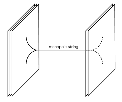
Figure 8: A schematic depiction of the magnetic monopole from the 5-dimensional point of view as a string stretched between separated domain walls.

Let us also remark, that this type of configuration has a direct analog in D-strings Diaconescu . Detailed study of these observations is a subject of a forthcoming work.

Lastly, in this work we have not discussed gravity for simplicity. However, an interesting direction for future study may be to consider Randall-Sundrum-like theory RS ; RS2 ; Eto:2002ns ; Arai:2002ph ; Eto:2003ut ; Eto:2003xq ; Eto:2003bn ; Eto:2004yk with multiple branes and investigate the issues of cosmological constant and the hierarchy problem there. Another and a perhaps more natural option is to employ position-dependent gravitational constant as a means to localize massless gravitons on multiple domain walls, thus creating the background dynamically. In this setting, it would be interesting to investigate spectra of graviphotons and fluctuations of domain walls as they are natural candidates for dark matter (for details of massive vector-like dark matter coming from brane oscillations see Clark1 ; Clark2 ). We plan to elaborate on this in the near future.

Appendix A Kaluza-Klein expansion of Abelian-Higgs model

Let us consider Abelian-Higgs model in 5 dimensions

$${\cal L}_{5}=-\frac{1}{4}F_{MN}F^{MN}+|D_{M}\phi|^{2}-\frac{\lambda^{2}}{4}\left(|\phi|^{2}-v^{2}\right)^{2}.$$ (A.1)

We compactify the fifth direction to $S^{1}/Z_{2}$ with radius $R$, and we impose periodicity to all fields as $f(y+2\pi R)=f(y)$. The KK expansions for the scalar and vector fields are given by

$$\phi(x,y) = v+\frac{1}{\sqrt{2\pi R}}\left(\eta^{(0)}(x)+i\sigma^{(0)}(x)\right)+\frac{1}{\sqrt{\pi R}}\sum_{k=1}^{\infty}\left(\eta^{(k)}(x)+i\sigma^{(k)}(x)\right)\cos\frac{k}{R}y,$$ (A.2)

$$A_{\mu}(x,y) = \frac{1}{\sqrt{2\pi R}}a_{\mu}^{(0)}(x)+\frac{1}{\sqrt{\pi R}}\sum_{k=1}^{\infty}a_{\mu}^{(k)}(x)\cos\frac{k}{R}y,$$ (A.3)

$$A_{y}(x,y) = \frac{1}{\sqrt{\pi R}}\sum_{k=1}^{\infty}a_{y}^{(k)}(x)\sin\frac{k}{R}y,$$ (A.4)

where we imposed that $\phi$ and $A_{\mu}$ are even whereas $A_{5}$ is odd for the orbifold parity. Let us write down the quadratic Lagrangian by inserting these KK expansions into ${\cal L}_{5}$ and integrating it by $y$. Then we get

$$-\frac{1}{4}\int^{2\pi R}_{0}dy~{}F_{\mu\nu}F^{\mu\nu}=-\frac{1}{4}f^{(0)}_{\mu\nu}f^{(0)\mu\nu}-\frac{1}{4}\sum_{k=1}^{\infty}f^{(k)}_{\mu\nu}f^{(k)\mu\nu},$$ (A.5)

with $f^{(k)}_{\mu\nu}=\partial_{\mu}a_{\nu}^{(k)}-\partial_{\nu}a_{\mu}^{(k)}$. We also have

$$-\frac{1}{2}\int^{2\pi R}_{0}dy~{}F_{\mu y}F^{\mu y}=\frac{1}{2}\sum_{k=1}^{\infty}\left(\partial_{\mu}a_{y}^{(k)}+\frac{k}{R}a_{\mu}^{(k)}\right)^{2}$$ (A.6)

where we have used

$$F_{\mu y}=\frac{1}{\sqrt{\pi R}}\sum_{k=1}^{\infty}\partial_{\mu}a_{y}^{(k)}\sin\frac{k}{R}y+\frac{1}{\sqrt{\pi R}}\sum_{k=1}^{\infty}\frac{k}{R}a_{\mu}^{(k)}\sin\frac{k}{R}y$$ (A.7)

We also have

$$\int_{0}^{2\pi R}dy~{}|D_{\mu}\phi|^{2} = \left(\partial_{\mu}\eta^{(0)}\right)^{2}+(ev)^{2}\left(a_{\mu}^{(0)}+\frac{1}{ev}\partial_{\mu}\sigma^{(0)}\right)^{2}$$ (A.8)

$$+ \sum_{k=1}^{\infty}\left\{\left(\partial_{\mu}\eta^{(k)}\right)^{2}+(ev)^{2}\left(a_{\mu}^{(k)}+\frac{1}{ev}\partial_{\mu}\sigma^{(k)}\right)^{2}\right\},$$

$$\int_{0}^{2\pi R}dy~{}|D_{y}\phi|^{2} = -\sum_{k=1}^{\infty}\left\{\left(\frac{k}{R}\right)^{2}\eta^{(k)2}+(ev)^{2}\left(a_{y}^{(k)}-\frac{1}{ev}\frac{k}{R}\sigma^{(k)}\right)^{2}\right\},$$ (A.9)

where we have used

$$D_{\mu}\phi = \frac{1}{\sqrt{2\pi R}}\left\{\partial_{\mu}\eta^{(0)}+iev\left(a_{\mu}^{(0)}+\frac{1}{ev}\partial_{\mu}\sigma^{(0)}\right)\right\}$$ (A.10)

$$+ \frac{1}{\sqrt{\pi R}}\sum_{k=1}^{\infty}\left\{\partial_{\mu}\eta^{(k)}+iev\left(a_{\mu}^{(k)}+\frac{1}{ev}\partial_{\mu}\sigma^{(k)}\right)\right\}\cos\frac{k}{R}y+\cdots,$$

$$D_{y}\phi = -\frac{1}{\sqrt{\pi R}}\sum_{k=1}^{\infty}\left\{\frac{k}{R}\eta^{(k)}-iev\left(a_{y}^{(k)}-\frac{1}{ev}\frac{k}{R}\sigma^{(k)}\right)\right\}\sin\frac{k}{R}y+\cdots.$$ (A.11)

Finally, we have

$$\int_{0}^{2\pi R}dy~{}V=(\lambda v)^{2}\eta^{(0)2}+(\lambda v)^{2}\sum_{k=1}^{\infty}\eta^{(k)2}.$$ (A.12)

Putting everything together, we find the quadratic Lagrangian

$${\cal L}_{4D}^{(2)} = -\frac{1}{4}f^{(0)}_{\mu\nu}f^{(0)\mu\nu}+(ev)^{2}\left(a_{\mu}^{(0)}+\frac{1}{ev}\partial_{\mu}\sigma^{(0)}\right)^{2}$$ (A.13)

$$+ \left(\partial_{\mu}\eta^{(0)}\right)^{2}-(\lambda v)^{2}\eta^{(0)2}+\sum_{k=1}^{\infty}\left(\partial_{\mu}\eta^{(k)}\right)^{2}-\left[(\lambda v)^{2}+\left(\frac{k}{R}\right)^{2}\right]\eta^{(k)2}$$

$$- \frac{1}{4}\sum_{k=1}^{\infty}f^{(k)}_{\mu\nu}f^{(k)\mu\nu}+\frac{1}{2}\sum_{k=1}^{\infty}\left(\partial_{\mu}a_{y}^{(k)}+\frac{k}{R}a_{\mu}^{(k)}\right)^{2}$$

$$+ \sum_{k=1}^{\infty}(ev)^{2}\left(a_{\mu}^{(k)}+\frac{1}{ev}\partial_{\mu}\sigma^{(k)}\right)^{2}-\sum_{k=1}^{\infty}(ev)^{2}\left(a_{y}^{(k)}-\frac{1}{ev}\frac{k}{R}\sigma^{(k)}\right)^{2}.$$

One immediately sees that $\sigma^{(0)}$ and $a_{\mu}^{(0)}$ appear only in the combination $a_{\mu}^{(0)}+\frac{1}{ev}\partial_{\mu}\sigma^{(0)}$, namely $\sigma^{(0)}$ is absorbed by $a_{\mu}^{(0)}$, so that $a_{\mu}^{(0)}$ gets non-zero mass by the ordinary Higgs mechanism. In $R\to\infty$ limit, the KK tower becomes massless, and indeed all of $\sigma^{(k)}$ appears always with $a_{\mu}^{(k)}$. Namely, infinite number of four-dimensional zero modes $\sigma^{(k)}$ are eaten by the infinite number of four-dimensional massless gauge fields $a_{\mu}^{(k)}$. It is nothing but the Higgs mechanism in five dimensions. In order to untangle the mixing at finite $R$, let us add the gauge fixing term of the Feynman gauge

$${\cal L}_{\rm F} = -\frac{1}{2}\int_{0}^{2\pi R}dy~{}\left(\partial_{M}A^{M}-2ev\sigma\right)^{2}$$ (A.14)

$$= -\frac{1}{2}\int_{0}^{2\pi R}dy~{}\left\{\frac{1}{\sqrt{2\pi R}}\left(\partial^{\mu}a^{(0)}_{\mu}-2ev\sigma^{(0)}\right)+\frac{1}{\sqrt{\pi R}}\sum_{k=1}^{\infty}\left(\partial^{\mu}a^{(k)}_{\mu}-\frac{k}{R}a^{(k)}_{y}-2ev\sigma^{(k)}\right)\cos\frac{k}{R}\right\}^{2}$$

$$= -\frac{1}{2}\left(\partial^{\mu}a^{(0)}_{\mu}-2ev\sigma^{(0)}\right)^{2}-\frac{1}{2}\sum_{k=1}^{\infty}\left(\partial^{\mu}a^{(k)}_{\mu}-\frac{k}{R}a^{(k)}_{y}-2ev\sigma^{(k)}\right)^{2}\,,$$

where we have used

$$\partial^{\mu}A_{\mu} = \frac{1}{\sqrt{2\pi R}}\partial^{\mu}a^{(0)}_{\mu}+\frac{1}{\sqrt{\pi R}}\sum_{k=1}^{\infty}\partial^{\mu}a^{(k)}_{\mu}\cos\frac{k}{R}y\,,$$ (A.15)

$$\partial^{y}A_{y} = -\frac{1}{\sqrt{\pi R}}\sum_{k=1}^{\infty}\frac{k}{R}a^{(k)}_{y}\cos\frac{k}{R}y\,.$$ (A.16)

In conclusion, we have

$${\cal L}_{4D}^{(2)}+{\cal L}_{\rm F} = -\frac{1}{4}f^{(0)}_{\mu\nu}f^{(0)\mu\nu}-\frac{1}{2}\left(\partial_{\mu}a^{(0)}_{\mu}\right)^{2}+(ev)^{2}\left(a_{\mu}^{(0)}\right)^{2}$$ (A.17)

$$+ \left(\partial_{\mu}\sigma^{(0)}\right)^{2}-2(ev)^{2}\sigma^{(0)2}+\sum_{k=1}^{\infty}\left\{\left(\partial_{\mu}\sigma^{(k)}\right)^{2}-\left[2(ev)^{2}+\left(\frac{k}{R}\right)^{2}\right]\sigma^{(k)2}\right\}$$

$$+ \left(\partial_{\mu}\eta^{(0)}\right)^{2}-(\lambda v)^{2}\eta^{(0)2}+\sum_{k=1}^{\infty}\left\{\left(\partial_{\mu}\eta^{(k)}\right)^{2}-\left[(\lambda v)^{2}+\left(\frac{k}{R}\right)^{2}\right]\eta^{(k)2}\right\}$$

$$+ \sum_{k=1}^{\infty}\left\{-\frac{1}{4}\sum_{k=1}^{\infty}f^{(k)}_{\mu\nu}f^{(k)\mu\nu}+\frac{1}{2}\left[2(ev)^{2}+\left(\frac{k}{R}\right)^{2}\right]\left(a_{\mu}^{(k)}\right)^{2}\right\}$$

$$+ \frac{1}{2}\sum_{k=1}^{\infty}\left\{\left(\partial_{\mu}a_{y}^{(k)}\right)^{2}-\left[2(ev)^{2}+\left(\frac{k}{R}\right)^{2}\right]\left(a_{y}^{(k)}\right)^{2}\right\}\,.$$

Now we can read the mass spectrum as $\sqrt{2}\,ev$, $\sqrt{2(ev)^{2}+(k/R)^{2}}$, $\lambda v$, and $\sqrt{(\lambda v)^{2}+(k/R)^{2}}$. Thus, all the masses are of order $M_{5}=\{\lambda v,ev\}$ or higher than $M_{5}$. So, no lighter particles than $M_{5}$ do exist for any $R$. This is, of course, because we compactify the fifth direction. Note that the masses shift to $0$, $k/R$, $\lambda v$, and $\sqrt{(\lambda v)^{2}+(k/R)^{2}}$ when we turn off the gauge interaction $(e=0)$. The massless mode corresponds to NG for broken global $U(1)$ and the next lightest masses are $k/R$ at large $R$. In the scalar model (Goldstone model) those KK tower can be very light as $R$ increased, but once the gauge interaction turned on, their mass is lifted of order $M_{5}$.

Appendix B Identities for the effective Lagrangian

Calculation of the effective Lagrangians in Sec. V is greatly simplified by using a few useful identities described in this appendix.

Let us first consider a generic integral appearing in the kinetic terms of scalar fields, namely

$$\int\limits_{-\infty}^{\infty}\mathrm{d}y\,\mathrm{Tr}\bigl{[}D_{\mu}f(y\mathbf{1}_{5}-\mathbf{Y})D^{\mu}f(y\mathbf{1}_{5}-\mathbf{Y})\bigr{]}$$ (B.1)

where ${\mathcal{L}}_{\mathbf{Y}}\equiv[\mathbf{Y},\cdot]$ is a Lie derivative. The first step in evaluating this integral is to rewrite

$$f(X)=f(\partial_{\alpha})e^{\alpha X}\Big{|}_{a=0}\,,$$ (B.2)

which holds for any $f$ with a Taylor expansion around the origin. Since in all our calculations we only deal with entire functions, such as $\tanh(z)$ or $\mbox{sech}(z)$, this is clearly satisfied. The second step involves the famous Poincaré identity

$$\delta e^{X}e^{-X}=\frac{e^{{\mathcal{L}}_{X}}-1}{{\mathcal{L}}_{X}}(\delta X)\,.$$ (B.3)

This leads to

$$\int\limits_{-\infty}^{\infty}\mathrm{d}y\,\mathrm{Tr}\bigl{[}D_{\mu}f(y\mathbf{1}_{5}-\mathbf{Y})D^{\mu}f(y\mathbf{1}_{5}-\mathbf{Y})\bigr{]}=$$ (B.4)

$$\int\limits_{-\infty}^{\infty}\mathrm{d}y\,\mathrm{Tr}\Bigl{[}f(\partial_{\alpha})f(\partial_{\beta})e^{(\alpha+\beta)(y\mathbf{1}_{5}-\mathbf{Y})}\frac{e^{\alpha{\mathcal{L}}_{\mathbf{Y}}}-1}{{\mathcal{L}}_{\mathbf{Y}}}\bigl{(}D_{\mu}\mathbf{Y}\bigr{)}\frac{1-e^{-\beta{\mathcal{L}}_{\mathbf{Y}}}}{{\mathcal{L}}_{\mathbf{Y}}}\bigl{(}D^{\mu}\mathbf{Y}\bigr{)}\Bigr{]}_{\alpha,\beta=0}$$ (B.5)

Now we can formally shift the integration variable as $y\mathbf{1}_{5}-\mathbf{Y}\to y\mathbf{1}_{5}$. This can be established more rigorously by first diagonalising the matrix $e^{(\alpha+\beta)(y\mathbf{1}_{5}-\mathbf{Y})}$ and rewriting the integral as a sum of integrals for each diagonal element. We can then shift the integration variable to absorb each diagonal element of $\mathbf{Y}$ separately. Since there is no other $y$-dependent term in the above integral, this amounts to the shift $y\mathbf{1}_{5}-\mathbf{Y}\to y\mathbf{1}_{5}$, as claimed.

Further, we will use the fact

$$f(\partial_{\alpha})e^{\alpha y}\Big{|}_{\alpha=0}=f(\partial_{\alpha}+y)\Big{|}_{\alpha=0}$$ (B.6)

and the properties of the trace to get

$$\int\limits_{-\infty}^{\infty}\mathrm{d}y\,\mathrm{Tr}\Bigl{[}f(\partial_{\alpha}+y\mathbf{1}_{5})f(\partial_{\beta}+y\mathbf{1}_{5})\frac{e^{\alpha{\mathcal{L}}_{\mathbf{Y}}}-1}{{\mathcal{L}}_{\mathbf{Y}}}\frac{e^{\beta{\mathcal{L}}_{\mathbf{Y}}}-1}{{\mathcal{L}}_{\mathbf{Y}}}\bigl{(}D_{\mu}\mathbf{Y}\bigr{)}D^{\mu}\mathbf{Y}\Bigr{]}_{\alpha,\beta=0}\,.$$ (B.7)

This leads to the final result

$$\int\limits_{-\infty}^{\infty}\mathrm{d}y\,\mathrm{Tr}\bigl{[}D_{\mu}f(y\mathbf{1}_{5}-\mathbf{Y})D^{\mu}f(y\mathbf{1}_{5}-\mathbf{Y})\bigr{]}=\mathrm{Tr}\Bigl{[}g\bigl{(}{\mathcal{L}}_{\mathbf{Y}}\bigr{)}\bigl{(}D_{\mu}\mathbf{Y}\bigr{)}D^{\mu}\mathbf{Y}\Bigr{]}\,,$$ (B.8)

where

$$g(\alpha)\equiv\int\limits_{-\infty}^{\infty}\mathrm{d}y\,\Bigl{(}\frac{f(y+\alpha)-f(y)}{\alpha}\Bigr{)}^{2}\,.$$ (B.9)

Let us also mention an identity relevant to our calculation of the moduli metric. If we decompose an adjoint field $Y$ as $Y=Y_{i}T_{i}$, where $T_{i}$ are generator of the $SU(N)$ algebra with the standard normalization

$$\bigl{[}T_{i},T_{j}\bigr{]}=if_{ijk}T_{k}\,,\hskip 14.22636pt\mathrm{Tr}\bigl{[}T_{i}T_{j}\bigr{]}=\frac{1}{2}\delta_{ij}\,,$$ (B.10)

it is easy to show the following

$$g({\mathcal{L}}_{\mathbf{Y}})\bigl{(}T_{i}\bigr{)}=g\bigl{(}i\mathbf{\tilde{Y}}\bigr{)}_{ij}T_{j}\,,$$ (B.11)

where $\mathbf{\tilde{Y}}_{ij}=f_{ijk}Y_{k}$. This simply comes out as a result of Taylor expanding the left side of the identity and repeatedly using the commutation relation for the generators.

References

- (1) E. Witten, “Dynamical Breaking of Supersymmetry,” Nucl. Phys. B 188 (1981) 513.
- (2) S. Dimopoulos and H. Georgi, “Softly Broken Supersymmetry and SU(5),” Nucl. Phys. B 193 (1981) 150.
- (3) N. Sakai, “Naturalness in Supersymmetric Guts,” Z. Phys. C 11 (1981) 153.
- (4) S. Dimopoulos, S. Raby and F. Wilczek, “Supersymmetry and the Scale of Unification,” Phys. Rev. D 24 (1981) 1681.
- (5) S. Weinberg, “Implications of Dynamical Symmetry Breaking: An Addendum,” Phys. Rev. D 19 (1979) 1277.
- (6) L. Susskind, “Dynamics of Spontaneous Symmetry Breaking in the Weinberg-Salam Theory,” Phys. Rev. D 20 (1979) 2619.
- (7) N. Arkani-Hamed, S. Dimopoulos and G. R. Dvali, “The Hierarchy problem and new dimensions at a millimeter,” Phys. Lett. B 429 (1998) 263 [hep-ph/9803315].
- (8) L. Randall and R. Sundrum, “A Large mass hierarchy from a small extra dimension,” Phys. Rev. Lett. 83 (1999) 3370 [hep-ph/9905221].
- (9) L. Randall and R. Sundrum, “An Alternative to compactification,” Phys. Rev. Lett. 83 (1999) 4690 [hep-th/9906064].
- (10) N. Arkani-Hamed and M. Schmaltz, “Hierarchies without symmetries from extra dimensions,” Phys. Rev. D 61 (2000) 033005 [hep-ph/9903417].
- (11) I. Antoniadis, N. Arkani-Hamed, S. Dimopoulos and G. R. Dvali, “New dimensions at a millimeter to a Fermi and superstrings at a TeV,” Phys. Lett. B 436 (1998) 257 doi:10.1016/S0370-2693(98)00860-0 [hep-ph/9804398].
- (12) V. A. Rubakov and M. E. Shaposhnikov, “Do We Live Inside a Domain Wall?,” Phys. Lett. 125B (1983) 136.
- (13) G. R. Dvali and M. A. Shifman, “Domain walls in strongly coupled theories,” Phys. Lett. B 396 (1997) 64 [Erratum-ibid. B 407 (1997) 452] [arXiv:hep-th/9612128].
- (14) N. Maru and N. Sakai, “Localized gauge multiplet on a wall,” Prog. Theor. Phys. 111 (2004) 907 [arXiv:hep-th/0305222].
- (15) C. Germani, “Spontaneous localization on a brane via a gravitational mechanism,” Phys. Rev. D 85 (2012) 055025 doi:10.1103/PhysRevD.85.055025 [arXiv:1109.3718 [hep-ph]].
- (16) G. R. Dvali, G. Gabadadze and M. A. Shifman, “(Quasi)localized gauge field on a brane: Dissipating cosmic radiation to extra dimensions?,” Phys. Lett. B 497 (2001) 271 [hep-th/0010071].
- (17) S. L. Dubovsky and V. A. Rubakov, “On models of gauge field localization on a brane,” Int. J. Mod. Phys. A 16 (2001) 4331 [hep-th/0105243].
- (18) E. K. Akhmedov, “Dynamical localization of gauge fields on a brane,” Phys. Lett. B 521 (2001) 79 [hep-th/0107223].
- (19) K. Ohta and N. Sakai, “Non-Abelian Gauge Field Localized on Walls with Four-Dimensional World Volume,” Prog. Theor. Phys. 124 (2010) 71 Erratum: [Prog. Theor. Phys. 127 (2012) 1133] [arXiv:1004.4078 [hep-th]].
- (20) N. Seiberg, “Five-dimensional SUSY field theories, nontrivial fixed points and string dynamics,” Phys. Lett. B 388 (1996) 753 [hep-th/9608111].
- (21) D. R. Morrison and N. Seiberg, “Extremal transitions and five-dimensional supersymmetric field theories,” Nucl. Phys. B 483 (1997) 229 [hep-th/9609070].
- (22) M. Arai, F. Blaschke, M. Eto and N. Sakai, “Matter Fields and Non-Abelian Gauge Fields Localized on Walls,” PTEP 2013 (2013) 013B05 [arXiv:1208.6219 [hep-th]].
- (23) M. Arai, F. Blaschke, M. Eto and N. Sakai, “Stabilizing matter and gauge fields localized on walls,” PTEP 2013 (2013) no.9, 093B01 [arXiv:1303.5212 [hep-th]].
- (24) M. Eto, T. Fujimori, M. Nitta, K. Ohashi and N. Sakai, “Domain walls with non-Abelian clouds,” Phys. Rev. D 77 (2008) 125008 [arXiv:0802.3135 [hep-th]].
- (25) M. Eto, T. Fujimori, M. Nitta, K. Ohashi and N. Sakai, “Domain walls with non-Abelian orientational moduli,” J. Phys. Conf. Ser. 222 (2010) 012006 [arXiv:0912.3590 [hep-th]].
- (26) N. S. Manton, “A Remark on the Scattering of BPS Monopoles,” Phys. Lett. 110B (1982) 54.
- (27) S. M. Carroll and M. Trodden, “Dirichlet topological defects,” Phys. Rev. D 57 (1998) 5189 [hep-th/9711099].
- (28) M. Bowick, A. De Felice and M. Trodden, “The Shapes of Dirichlet defects,” JHEP 0310 (2003) 067 [hep-th/0306224].
- (29) E. Witten, “Branes and the dynamics of QCD,” Nucl. Phys. B 507 (1997) 658 [hep-th/9706109].
- (30) I. I. Kogan, A. Kovner and M. A. Shifman, “More on supersymmetric domain walls, N counting and glued potentials,” Phys. Rev. D 57 (1998) 5195 [hep-th/9712046].
- (31) A. Campos, K. Holland and U. J. Wiese, “Complete wetting in supersymmetric QCD or why QCD strings can end on domain walls,” Phys. Rev. Lett. 81 (1998) 2420 [hep-th/9805086].
- (32) M. Arai, F. Blaschke and M. Eto, “BPS Boojums in N=2 supersymmetric gauge theories,” arXiv:1603.00447 [hep-th].
- (33) M. Arai, F. Blaschke and M. Eto, “BPS Boojums in N=2 supersymmetric gauge theories II,” arXiv:1612.00306 [hep-th].
- (34) M. Shifman and A. Yung, “NonAbelian string junctions as confined monopoles,” Phys. Rev. D 70 (2004) 045004 [hep-th/0403149].
- (35) N. Sakai and D. Tong, “Monopoles, vortices, domain walls and D-branes: The Rules of interaction,” JHEP 0503 (2005) 019 [hep-th/0501207].
- (36) D. Tong, “D-branes in field theory,” JHEP 0602 (2006) 030 [hep-th/0512192].
- (37) M. Shifman and A. Yung, “Domain walls and flux tubes in N=2 SQCD: D-brane prototypes,” Phys. Rev. D 67 (2003) 125007 [hep-th/0212293].
- (38) M. Shifman and A. Yung, “Localization of nonAbelian gauge fields on domain walls at weak coupling (D-brane prototypes II),” Phys. Rev. D 70 (2004) 025013 [hep-th/0312257].
- (39) A. Hanany and D. Tong, “Vortices, instantons and branes,” JHEP 0307 (2003) 037 [hep-th/0306150].
- (40) C. Montonen, “On Solitons with an Abelian Charge in Scalar Field Theories. 1. Classical Theory and Bohr-Sommerfeld Quantization,” Nucl. Phys. B 112 (1976) 349.
- (41) S. Sarkar, S. E. Trullinger and A. R. Bishop, “Solitary Wave Solution for a Complex One-Dimensional Field,” Phys. Lett. A 59 (1976) 255.
- (42) H. Ito, “Kink Energy Sum Rule In A Two Component Scalar Field Model Of (1+1)-dimensions,” Phys. Lett. A 112 (1985) 119.
- (43) M. Eto, T. Fujimori, M. Nitta, K. Ohashi and N. Sakai, “Higher Derivative Corrections to Non-Abelian Vortex Effective Theory,” Prog. Theor. Phys. 128 (2012) 67 [arXiv:1204.0773 [hep-th]].
- (44) M. Eto and Y. Murakami, “Dyonic non-Abelian vortex strings in supersymmetric and non-supersymmetric theories — tensions and higher derivative corrections,” JHEP 1503, 078 (2015) doi:10.1007/JHEP03(2015)078 [arXiv:1412.7892 [hep-th]].
- (45) E. R. C. Abraham and P. K. Townsend, “Q kinks,” Phys. Lett. B 291, 85 (1992). doi:10.1016/0370-2693(92)90122-K
- (46) J. P. Gauntlett, R. Portugues, D. Tong and P. K. Townsend, “D-brane solitons in supersymmetric sigma models,” Phys. Rev. D 63, 085002 (2001) doi:10.1103/PhysRevD.63.085002 [hep-th/0008221].
- (47) M. Eto, “J-kink domain walls and the DBI action,” JHEP 1506, 160 (2015) doi:10.1007/JHEP06(2015)160 [arXiv:1504.00753 [hep-th]].
- (48) M. Eto and K. Hashimoto, “Speed limit in internal space of domain walls via all-order effective action of moduli motion,” Phys. Rev. D 93 (2016) no.6, 065058 [arXiv:1508.00433 [hep-th]].
- (49) M. Arai, F. Blaschke, M. Eto and N. Sakai, “Grand Unified Brane World Scenario,” [arXiv:1703.00351 [hep-th]].
- (50) N. Maru, N. Sakai, Y. Sakamura and R. Sugisaka, “Simple SUSY breaking mechanism by coexisting walls,” Nucl. Phys. B 616, 47 (2001) doi:10.1016/S0550-3213(01)00435-7 [hep-th/0107204].
- (51) N. Maru, N. Sakai, Y. Sakamura and R. Sugisaka, “SUSY breaking by overlap of wave functions in coexisting walls,” Phys. Lett. B 496, 98 (2000) doi:10.1016/S0370-2693(00)01285-5 [hep-th/0009023].
- (52) G. ’t Hooft, “Magnetic Monopoles in Unified Gauge Theories,” Nucl. Phys. B 79 (1974) 276.
- (53) A. M. Polyakov, “Particle Spectrum in the Quantum Field Theory,” JETP Lett. 20 (1974) 194 [Pisma Zh. Eksp. Teor. Fiz. 20 (1974) 430]
- (54) D. E. Diaconescu, “D-branes, monopoles and Nahm equations,” Nucl. Phys. B 503 (1997) 220 [hep-th/9608163].
- (55) M. Eto, N. Maru, N. Sakai and T. Sakata, “Exactly solved BPS wall and winding number in N=1 supergravity,” Phys. Lett. B 553, 87 (2003) doi:10.1016/S0370-2693(02)03187-8 [hep-th/0208127].
- (56) M. Arai, S. Fujita, M. Naganuma and N. Sakai, “Wall solution with weak gravity limit in five-dimensional supergravity,” Phys. Lett. B 556 (2003) 192 doi:10.1016/S0370-2693(03)00107-2 [hep-th/0212175].
- (57) M. Eto, S. Fujita, M. Naganuma and N. Sakai, “BPS Multi-walls in five-dimensional supergravity,” Phys. Rev. D 69 (2004) 025007 [hep-th/0306198].
- (58) M. Eto, N. Maru and N. Sakai, “Stability and fluctuations on walls in N=1 supergravity,” Nucl. Phys. B 673, 98 (2003) doi:10.1016/j.nuclphysb.2003.09.025 [hep-th/0307206].
- (59) M. Eto and N. Sakai, “Solvable models of domain walls in N = 1 supergravity,” Phys. Rev. D 68, 125001 (2003) doi:10.1103/PhysRevD.68.125001 [hep-th/0307276].
- (60) M. Eto, N. Maru and N. Sakai, “Radius stabilization in a supersymmetric warped compactification,” Phys. Rev. D 70, 086002 (2004) doi:10.1103/PhysRevD.70.086002 [hep-th/0403009].
- (61) T. E. Clark, S. T. Love, C. Xiong, M. Nitta and T. ter Veldhuis, “Colliders and Brane Vector Phenomenology,” Phys. Rev. D 78 (2008) 115004 [arXiv:0809.3999 [hep-ph]].
- (62) T. E. Clark, S. T. Love, M. Nitta, T. ter Veldhuis and C. Xiong, “Brane vector phenomenology,” Phys. Lett. B 671 (2009) 383 [arXiv:0709.4023 [hep-th]].