Detecting Adversarial Samples from Artifacts

Abstract

Deep neural networks (DNNs) are powerful nonlinear architectures that are known to be robust to random perturbations of the input. However, these models are vulnerable to adversarial perturbations—small input changes crafted explicitly to fool the model. In this paper, we ask whether a DNN can distinguish adversarial samples from their normal and noisy counterparts. We investigate model confidence on adversarial samples by looking at Bayesian uncertainty estimates, available in dropout neural networks, and by performing density estimation in the subspace of deep features learned by the model. The result is a method for implicit adversarial detection that is oblivious to the attack algorithm. We evaluate this method on a variety of standard datasets including MNIST and CIFAR-10 and show that it generalizes well across different architectures and attacks. Our findings report that 85-93% ROC-AUC can be achieved on a number of standard classification tasks with a negative class that consists of both normal and noisy samples.

1 Introduction

Deep neural networks (DNNs) are machine learning techniques that impose a hierarchical architecture consisting of multiple layers of nonlinear processing units. In practice, DNNs achieve state-of-the-art performance for a variety of generative and discriminative learning tasks from domains including image processing, speech recognition, drug discovery and genomics (LeCun et al., 2015).

Although DNNs are known to be robust to noisy inputs (Fawzi et al., 2016), they have been shown to be vulnerable to specially-crafted adversarial samples (Szegedy et al., 2014; Goodfellow et al., 2015). These samples are constructed by taking a normal sample and perturbing it, either at once or iteratively, in a direction that maximizes the chance of misclassification. Figure 1 shows some examples of adversarial MNIST images alongside noisy images of equivalent perturbation size. Adversarial attacks which require only small perturbations to the original inputs can induce high-efficacy DNNs to misclassify at a high rate. Some adversarial samples can also induce a DNN to output a specific target class (Papernot et al., 2016b). The vulnerability of DNNs to such adversarial attacks highlights important security and performance implications for these models (Papernot et al., 2016b). Consequently, significant effort is ongoing to understand and explain adversarial samples and to design defenses against them (Szegedy et al., 2014; Goodfellow et al., 2015; Papernot et al., 2016c; Tanay & Griffin, 2016; Metzen et al., 2017).

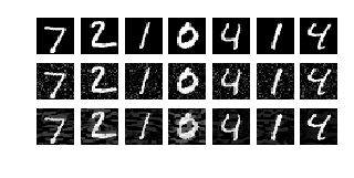
Figure 1: Examples of normal (top), noisy (middle) and adversarial (bottom) MNIST samples for a convnet. Adversarial samples were crafted via the Basic Iterative Method (Kurakin et al., 2017) and fool the model into misclassifying 100% of the time.

Using the intuition that adversarial samples lie off the true data manifold, we devise two novel features that can be used to detect adversarial samples:

• Density estimates, calculated with the training set in the feature space of the last hidden layer. These are meant to detect points that lie far from the data manifold.

• Bayesian uncertainty estimates, available in dropout neural networks. These are meant to detect when points lie in low-confidence regions of the input space, and can detect adversarial samples in situations where density estimates cannot.

When both of these features are used as inputs to a simple logistic regression model, we observe effective detection of adversarial samples, achieving an ROC-AUC of $92.6\%$ on the MNIST dataset with both noisy and normal samples as the negative class. In Section 2 we provide the relevant background information for our approach, and in Section 3 we briefly review a few state-of-the-art adversarial attacks. Then, we introduce the intuition for our approach in Section 4, with a discussion of manifolds and Bayesian uncertainty. This leads us to our results and conclusions in Sections 5 and 6.

2 Background

While neural networks are known to be robust to random noise (Fawzi et al., 2016), they have been shown to be vulnerable to adversarially-crafted perturbations (Szegedy et al., 2014; Goodfellow et al., 2015; Papernot et al., 2016b). Specifically, an adversary can use information about the model to craft small perturbations that fool the network into misclassifying their inputs. In the context of object classification, these perturbations are often imperceptible to the human eye, yet they can force the model to misclassify with high model confidence.

A number of works have attempted to explain the vulnerability of DNNs to adversarial samples. Szegedy et al. (2014) offered a simple preliminary explanation for the phenomenon, arguing that low-probability adversarial “pockets” are densely distributed in input space. As a result, they argued, every point in image space is close to a vast number of adversarial points and can be easily manipulated to achieve a desired model outcome. Goodfellow et al. (2015) argued that it is a result of the linear nature of deep classifiers. Although this explanation has been the most well-accepted in the field, it was recently weakened by counterexamples (Tanay & Griffin, 2016). Tanay & Griffin (2016) introduced the ‘boundary tilting’ perspective, suggesting instead that adversarial samples lie in regions where the classification boundary is close to the manifold of training data.

Research in adversarial attack defense generally falls within two categories: first, methods for improving the robustness of classifiers to current attacks, and second, methods for detecting adversarial samples in the wild. Goodfellow et al. (2015) proposed augmenting the training loss function with an additional adversarial term to improve the robustness of these models to a specific adversarial attack. Defensive distillation (Papernot et al., 2016c) is another recently-introduced technique which involves training a DNN with the softmax outputs of another neural network that was trained on the training data, and can be seen as a way of preventing the network from fitting too tightly to the data. Defensive distillation is effective against the attack of Papernot et al. (2016b). However, Carlini & Wagner (2016) showed that defensive distillation is easily broken with a modified attack.

On the detection of adversarial samples, Metzen et al. (2017) proposed augmenting a DNN with an additional “detector” subnetwork, trained on normal and adversarial samples. Although the authors show compelling performance results on a number of state-of-the-art adversarial attacks, one major drawback is that the detector subnetwork must be trained on generated adversarial samples. This implicitly trains the detector on a subset of all possible adversarial attacks; we do not know how comprehensive this subset is, and future attack modifications may be able to surmount the system. The robustness of this technique to random noise is not currently known.

3 Adversarial Attacks

The typical goal of an adversary is to craft a sample that looks similar to a normal sample, and yet that gets misclassified by the target model. In the realm of image classification, this amounts to finding a small perturbation that, when added to a normal image, causes the target model to misclassify the sample, but remains correctly classified by the human eye. For a given input image $x$, the goal is to find a minimal perturbation $\eta$ such that the adversarial input $\tilde{x}=x+\eta$ is misclassified. A significant number of adversarial attacks satisfying this goal have been introduced in recent years. This allows us a wide range of attacks to choose from in our investigation. Here, we introduce some of the most well-known and most recent attacks.

Fast Gradient Sign Method (FGSM): Goodfellow et al. (2015) introduced the Fast Gradient Sign Method for crafting adversarial perturbations using the derivative of the model’s loss function with respect to the input feature vector. Given a base input, the approach is to perturb each feature in the direction of the gradient by magnitude $\epsilon$, where $\epsilon$ is a parameter that determines perturbation size. For a model with loss $J(\Theta,x,y)$, where $\Theta$ represents the model parameters, $x$ is the model input, and $y$ is the label of $x$, the adversarial sample is generated as

$$x^{*}=x+\epsilon\operatorname{sign}(\nabla_{x}J(\Theta,x,y)).$$

With small $\epsilon$, it is possible to fool DNNs trained for the MNIST and CIFAR-10 classification tasks with high success rate (Goodfellow et al., 2015).

Basic Iterative Method (BIM): Kurakin et al. (2017) proposed an iterative version of FGSM called the Basic Iterative Method. This is a straightforward extension; instead of merely applying adversarial noise $\eta$ once with one parameter $\epsilon$, apply it many times iteratively with small $\epsilon$. This gives a recursive formula:

$$x^{*}_{0} = x,$$

$$x^{*}_{i} = \operatorname{clip}_{x,\epsilon}(x^{*}_{i-1}+\epsilon\operatorname{sign}(\nabla_{x^{*}_{i-1}}J(\Theta,x^{*}_{i-1},y))).$$

Here, $\operatorname{clip}_{x,\epsilon}(\cdot)$ represents a clipping of the values of the adversarial sample such that they are within an $\epsilon$-neighborhood of the original sample $x$. This approach is convenient because it allows extra control over the attack. For instance, one can control how far past the classification boundary a sample is pushed: one can terminate the loop on the iteration when $x^{*}_{i}$ is first misclassified, or add additional noise beyond that point.

The basic iterative method was shown to be typically more effective than the FGSM attack on ImageNet images (Kurakin et al., 2017).

Jacobian-based Saliency Map Attack (JSMA): Papernot et al. (2016b) proposed a simple iterative method for targeted misclassification. By exploiting the forward derivative of a DNN, one can find an adversarial perturbation that will force the model to misclassify into a specific target class. For an input $x$ and a neural network $F$, the output for class $j$ is denoted $F_{j}(x)$. To achieve a target class $t$, $F_{t}(X)$ must be increased while the probabilities $F_{j}(X)$ of all other classes $j\neq t$ decrease, until $t=\operatorname{arg\,max}_{j}F_{j}(X)$. This is accomplished by exploiting the adversarial saliency map, which is defined as

$$S(X,t)[i]=\begin{cases}0,\text{ if }\ \frac{\partial F_{t}(X)}{\partial X_{i}}<0\text{ or }\sum_{j\neq t}\frac{\partial F_{j}(X)}{\partial X_{i}}>0\\ (\frac{\partial F_{t}(X)}{\partial X_{i}})|\sum_{j\neq t}\frac{\partial F_{j}(X)}{\partial X_{i}}|,\text{ otherwise}\end{cases}$$

for an input feature $i$. Starting with a normal sample $x$, we locate the pair of features $\{i,j\}$ that maximize $S(X,t)[i]+S(X,t)[j]$, and perturb each feature by a constant offset $\epsilon$. This process is repeated iteratively until the target misclassification is achieved. This method can effectively produce MNIST samples that are correctly classified by human subjects but misclassified into a specific target class by a DNN with high success rate.

Carlini & Wagner (C&W): Carlini & Wagner (2016) recently introduced a technique that is able to overcome defensive distillation. In fact, their technique encompasses a range of attacks, all cast through the same optimization framework. This results in three powerful attacks, each for a different distance metric: an $L_{2}$ attack, an $L_{0}$ attack, and an $L_{\infty}$ attack. For the $L_{0}$ attack, which we will consider in this paper, the perturbation $\delta$ is defined in terms of an auxiliary variable $\omega$ as

$$\delta^{*}_{i}=\frac{1}{2}\left(\operatorname{tanh}(\omega_{i}+1)\right)-x_{i}.$$

Then, to find $\delta^{*}$ (an ‘unrestricted perturbation’), we optimize over $\omega$:

$$\operatorname{min}_{\omega}\left\|\frac{1}{2}\left(\operatorname{tanh}(\omega)+1\right)-x\right\|^{2}_{2}+cf\left(\frac{1}{2}\operatorname{tanh}(\omega)+1\right)$$

where $f(\cdot)$ is an objective function based on the hinge loss:

$$f(x)=\operatorname{max}(\operatorname{max}\{Z(x)_{i}:i\neq t\}-Z(x)_{t},-\kappa).$$

Here, $Z(x)_{i}$ is the pre-softmax output for class $i$, $t$ is the target class, and $\kappa$ is a parameter that controls the confidence with which the misclassification occurs.

Finally, to produce the adversarial sample $x^{*}=x+\delta$, we convert the unrestricted perturbation $\delta^{*}$ to a restricted perturbation $\delta$, in order to reduce the number of changed pixels. By calculating the gradient $\nabla f(x+\delta^{*})$, we may identify those pixels $\delta^{*}_{i}$ with little importance (small gradient values) and take $\delta_{i}=0$; otherwise, for larger gradient values we take $\delta_{i}=\delta^{*}_{i}$. This allows an effective attack with few modified pixels, thus helping keep the norm of $\delta$ low.

These three attacks were shown to be particularly effective in comparison to other attacks against networks trained with defensive distillation, achieving adversarial sample generation success rates of 100% where other techniques were not able to top 1%.

4 Artifacts of Adversarial Samples

(a) Two simple 2D submanifolds.

(b) One submanifold has a ‘pocket’.

(c) Nearby 2D submanifolds.

Figure 2: (a): The adversarial sample $x^{*}$ is generated by moving off the ‘-’ submanifold and across the decision boundary (black dashed line), but $x^{*}$ still lies far from the ‘+’ submanifold. (b): the ‘+’ submanifold has a ‘pocket’, as in Szegedy et al. (2014). $x^{*}$ lies in the pocket, presenting significant difficulty for detection. (c): the adversarial sample $x^{*}$ is near both the decision boundary and both submanifolds.

Each of these adversarial sample generation algorithms are able to change the predicted label of a point without changing the underlying true label: humans will still correctly classify an adversarial sample, but models will not. This can be understood from the perspective of the manifold of training data. Many high-dimensional datasets, such as images, are believed to lie on a low-dimensional manifold (Lee & Verleysen, 2007). Gardner et al. (2015) recently showed that by carefully traversing the data manifold, one can change the underlying true label of an image. The intuition is that adversarial perturbations—which do not constitute meaningful changes to the input—must push samples off of the data manifold. Tanay & Griffin (2016) base their investigation of adversarial samples on the assumption that adversarial samples lie near class boundaries that are close to the edge of a data submanifold. Similarly, Goodfellow et al. (2015) demonstrate that DNNs perform correctly only near the small manifold of training data. Therefore, we base our work here on the assumption that adversarial samples do not lie on the data manifold.

If we accept that adversarial samples are points that would not arise naturally, then we can assume that a technique to generate adversarial samples will, from a source point $x$ with class $c_{x}$, typically generate an adversarial sample $x^{*}$ that does not lie on the manifold and is classified incorrectly as $c_{x^{*}}$. If $x^{*}$ lies off of the data manifold, we may split into three possible situations:

1. $x^{*}$ is far away from the submanifold of $c_{x^{*}}$.

2. $x^{*}$ is near the submanifold $c_{x^{*}}$ but not on it, and $x^{*}$ is far from the classification boundary separating classes $c_{x}$ and $c_{x^{*}}$.

3. $x^{*}$ is near the submanifold $c_{x^{*}}$ but not on it, and $x^{*}$ is near the classification boundary separating classes $c_{x}$ and $c_{x^{*}}$.

Figures 2(a) through 2(c) show simplified example illustrations for each of these three situations in a two-dimensional binary classification setting.

4.1 Density Estimation

If we have an estimate of what the submanifold corresponding to data with class $c_{x^{*}}$ is, then we can determine whether $x^{*}$ falls near this submanifold after observing the prediction $c_{x^{*}}$. Following the intuition of Gardner et al. (2015) and hypotheses of Bengio et al. (2013), the deeper layers of a DNN provide more linear and ‘unwrapped’ manifolds to work with than input space; therefore, we may use this idea to model the submanifolds of each class by performing kernel density estimation in the feature space of the last hidden layer.

The standard technique of kernel density estimation can, given the point $x$ and the set $X_{t}$ of training points with label $t$, provide a density estimate $\hat{f}(x)$ that can be used as a measure of how far $x$ is from the submanifold for $t$. Specifically,

$$\hat{f}(x)=\frac{1}{|X_{t}|}\sum_{x_{i}\in X_{t}}k(x_{i},x)$$ (1)

where $k(\cdot,\cdot)$ is the kernel function, often chosen as a Gaussian with bandwidth $\sigma$:

$$k_{\sigma}(x,y)\sim\exp(-\|x-y\|^{2}/\sigma^{2}).$$ (2)

The bandwidth may typically be chosen as a value that maximizes the log-likelihood of the training data (Jones et al., 1996). A value too small will give rise to a ‘spiky’ density estimate with too many gaps (see Figure 3), but a value too large will give rise to an overly-smooth density estimate (see Figure 4). This also implies that the estimate is improved as the training set size $|X_{t}|$ increases, since we are able to use smaller bandwidths without the estimate becoming too ‘spiky.’

Figure 3: ‘spiky’ density estimate from a too-small bandwidth on 1-D points sampled from a bimodal distribution.

Figure 4: Overly smooth density estimate from a too-large bandwidth on 1-D points sampled from a bimodal distribution.

For the manifold estimate, we operate in the space of the last hidden layer. This layer provides a space of reasonable dimensionality in which we expect the manifold of our data to be simplified. If $\phi(x)$ is the last hidden layer activation vector for point $x$, then our density estimate for a point $x$ with predicted class $t$ is defined as

$$\hat{K}(x,X_{t})=\sum_{x_{i}\in X_{t}}k_{\sigma}(\phi(x),\phi(x_{i}))$$ (3)

where $X_{t}$ is the set of training points of class $t$, and $\sigma$ is the tuned bandwidth.

To validate our intuition about the utility of this density estimate, we perform a toy experiment using the BIM attack with a convnet trained on MNIST data. In Figure 5, we plot the density estimate of the source class and the final predicted class for each iteration of BIM. One can see that the adversarial sample moves away from a high density estimate region for the correct class, and towards a high density estimate region for the incorrect class. This matches our intuition: we expect the adversarial sample to leave the correct class manifold and move towards (but not onto) the incorrect class manifold.

Figure 5: Density estimate as a function of number of iterations of the BIM attack for a few MNIST sample points. The estimate decreases for the source class (blue) and increases for the incorrect class (red); usually the crossover point is near when the predicted class changes (black line).

While a density estimation approach can easily detect an adversarial point that is far from the $c_{x^{*}}$ submanifold, this strategy may not work well when $x^{*}$ is very near the $c_{x^{*}}$ submanifold. Therefore, we must investigate alternative approaches for those cases.

4.2 Bayesian Neural Network Uncertainty

Beyond distance-based metrics, another powerful tool to identify low-confidence regions of the input space is the uncertainty output of Bayesian models, e.g., the Gaussian process (Rasmussen & Williams, 2005). Gaussian processes assume a Gaussian prior over the set of all functions, $\mathcal{F}$, that can be used to map the input space to the output space. As observations ($x,y$) are made, only those functions $f\in\mathcal{F}$ are retained for which $f(x)=y$. For a new test point $x^{*}$, the prediction for each function $f$, $y^{*}=f(x^{*})$, is computed and the expected value over $y^{*}$ is the used as the final prediction. Simultaneously, the variance of the output values $y^{*}$ is also used as an indicator of the model’s uncertainty. Figure 6 illustrates how in simple cases, Bayesian uncertainty can provide additional information about model confidence not conveyed by distance metrics like a density estimate.

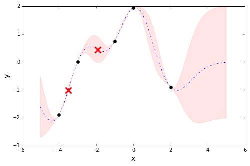
Figure 6: A simple 1-dimensional Gaussian process regression. The dashed line indicates the mean prediction and the shaded area indicates the 95% confidence interval. While two test points (red x’s) are equidistant from their nearest training points (black dots), their uncertainty estimates differ significantly.

Recently, Gal & Ghahramani (2015) proved that DNNs trained with dropout are equivalent to an approximation of the deep Gaussian process. As result, we can extract Bayesian uncertainty estimates from a wide range of DNN architectures without modification. Dropout, first introduced as a method to reduce overfitting when training DNNs (Srivastava et al., 2014), works by dropping hidden nodes from the network randomly with some probability $p$ during the training phase. During the testing phase, all nodes are kept, but the weights are scaled by $p$. Gal & Ghahramani (2015) showed that the dropout training objective converges to a minimization of the Kullback-Leibler divergence between an aproximate distribution and the posterior of a deep Gaussian process marginalized over its covariance function parameters. After iterating to convergence, uncertainty estimates can be extracted from dropout DNNs in the following manner.

We sample $T$ times from our distribution of network configurations, typically i.i.d. $Bernoulli(o_{l})$ for each layer $l$, and obtain parameters $\{W^{1},\cdots,W^{T}\}$. Here $W^{t}=\{W_{1}^{t},...,W_{L}^{t}\}$ are the $L$ weight matrices sampled at iteration $t$. Thereafter, we can evaluate a Monte Carlo estimate of the output, i.e. the first moment, as:

$$\mathbb{E}_{q(y^{*}|x^{*})}[y^{*}]\approx\frac{1}{T}\sum\limits_{i=1}^{T}\hat{y}^{*}(x^{*},W^{t}).$$ (4)

Similarly, we can evaluate the second moment with Monte Carlo estimation, leading us to an estimate of model variance

$$\mathbb{V}_{q(y^{*}|x^{*})}[y^{*}] \approx \tau^{-1}I_{D}$$ (5)

$$+\frac{1}{T}\sum\limits_{i=1}^{T}\hat{y}^{*}(x^{*},W^{t})^{T}\hat{y}^{*}(x^{*},W^{t})$$

$$-\mathbb{E}_{q(y^{*}|x^{*})}[y^{*}]^{T}\mathbb{E}_{q(y^{*}|x^{*})}[y^{*}]$$

where $\tau$ is our model precision.

Relying on the intuition that Bayesian uncertainty can be useful to identify adversarial samples, we make use of dropout variance values in this paper, setting $T=50$. As dropout on its own is known to be a powerful regularization technique (Srivastava et al., 2014), we use neural network models without weight decay, leaving $\tau^{-1}=0$. Thus, for a test sample $x^{*}$ and stochastic predictions $\{\hat{y}^{*}_{1},...,\hat{y}^{*}_{T}\}$, our uncertainty estimate $U(x^{*})$ can be computed as

$$U(x^{*})=\frac{1}{T}\sum\limits_{i=1}^{T}\hat{y_{i}^{*}}^{T}\hat{y_{i}^{*}}-\left(\frac{1}{T}\sum\limits_{i=1}^{T}\hat{y_{i}^{*}}\right)^{T}\left(\frac{1}{T}\sum\limits_{i=1}^{T}\hat{y_{i}^{*}}\right).$$ (6)

Because we use DNNs with one output node per class, we look at the mean of the uncertainty vector as a scalar representation of model uncertainty.

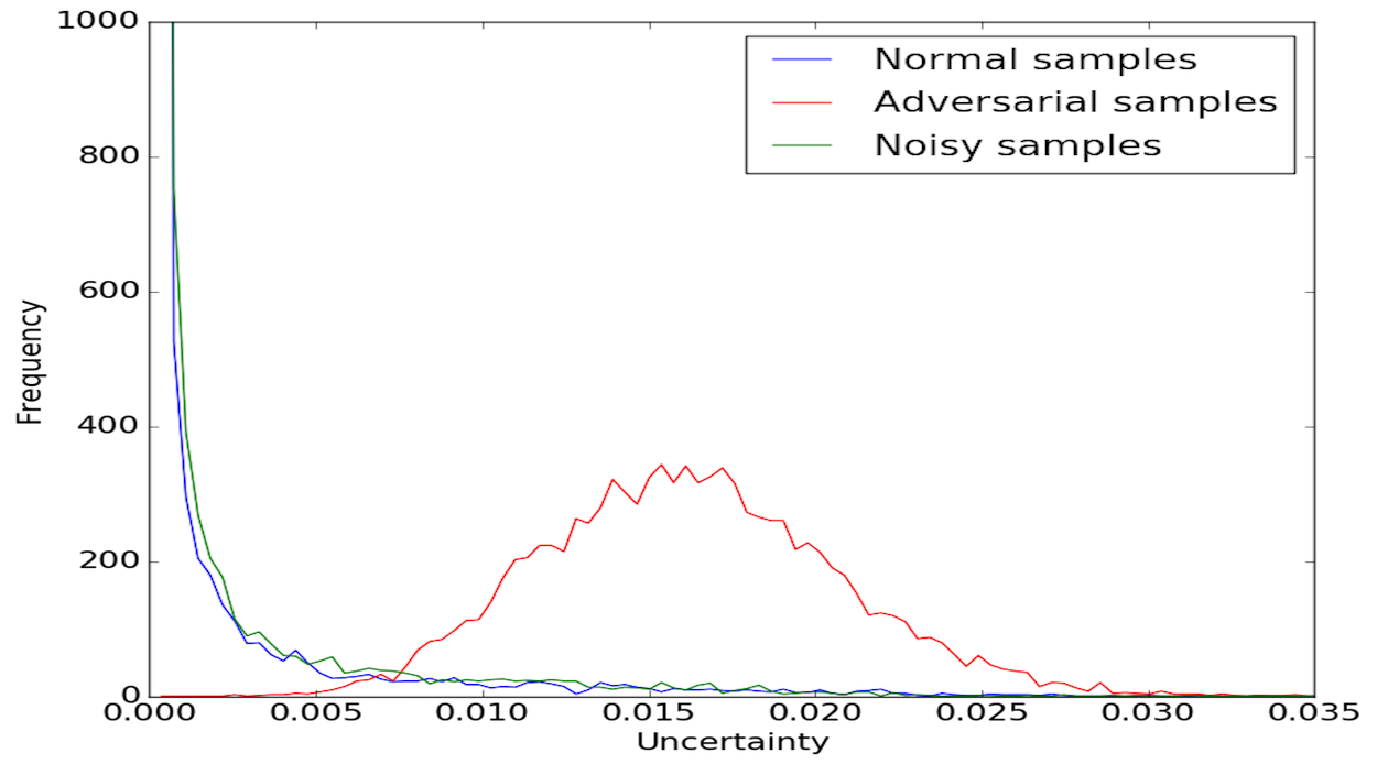
(a) BIM

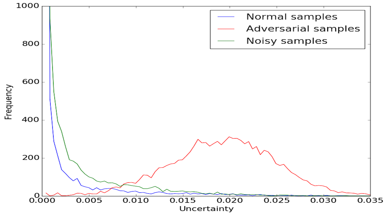
(b) JSMA

Figure 7: Model uncertainty distributions per sample type for MNIST. Distributions are based on a histogram with 100 bins.

To demonstrate the efficacy of our uncertainty estimates in detecting adversarial samples, we trained the LeNet convnet (LeCun et al., 1989) with a dropout rate of 0.5 applied after the last pooling layer and after the inner-product layer for MNIST classification. Figures 7(a) and 7(b) compare the distribution of Bayesian uncertainty for adversarial samples to those of normal samples and of noisy samples with equivalent perturbation size; both the BIM and JSMA cases are shown. Clearly, uncertainty distributions for adversarial samples are statistically distinct from normal and noisy samples, verifying our intuition.

5 Experiments

Dataset	FGSM		BIM-A		BIM-B		JSMA		C&W
	$L_{2}$	Acc.	$L_{2}$	Acc.	$L_{2}$	Acc.	$L_{2}$	Acc.	$L_{2}$	Acc.
MNIST	$6.22$	$5.87$%	$2.62$	$0.00$%	$5.37$	$0.00$%	$5.00$	$2.70$%	$4.71$	$0.79$%
CIFAR-10	$2.74$	$7.03$%	$0.48$	$0.57$%	$2.14$	$0.57$%	$3.45$	$0.20$%	$2.70$	$0.89$%
SVHN	$7.08$	$3.29$%	$0.83$	$0.00$%	$6.56$	$0.00$%	$2.96$	$0.32$%	$2.37$	$0.87$%

Table 1: Adversarial attack details. For each algorithm, the average $L_{2}$-norm of the perturbation is shown, as well as the model accuracy on the adversarial set.

In order to evaluate the proficiency of our density and uncertainty features for adversarial detection, we test these features on MNIST, CIFAR10, and SVHN. All pixels are scaled to floats in the range of [0, 1]. Our models achieve near state-of-the-art accuracy on the normal holdout sets for each dataset and are described in Section 5.1. In order to properly evaluate our method, we only perturb those test samples which were correctly classified by our models in their original states. An adversary would have no reason to perturb samples that are already misclassified.

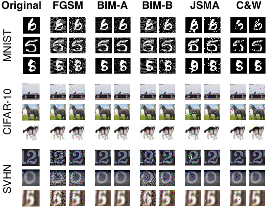
Figure 8: Some example images from MNIST, CIFAR-10 and SVHN. The original image is shown in the left-most column. For each attack, the left image is the adversarial sample and the right image is a corresponding noisy sample of equal perturbation size.

Sample	MNIST				CIFAR-10
Type	$\frac{u(x^{*})}{u(x)}>1$	$\frac{d(x^{*})}{d(x)}<1$	$\frac{u(x^{*})}{u(x^{n})}>1$	$\frac{d(x^{*})}{d(x^{n})}<1$	$\frac{u(x^{*})}{u(x)}>1$	$\frac{d(x^{*})}{d(x)}<1$	$\frac{u(x^{*})}{u(x^{n})}>1$	$\frac{d(x^{*})}{d(x^{n})}<1$
FGSM	$92.2$%	$95.6$%	$79.5$%	$90.0$%	$74.7$%	$70.1$%	$68.2$%	$69.6$%
BIM-A	$99.2$%	$98.0$%	$99.5$%	$98.7$%	$83.4$%	$76.4$%	$83.3$%	$76.8$%
BIM-B	$60.7$%	$90.5$%	$35.6$%	$86.7$%	$4.0$%	$98.8$%	$3.6$%	$99.1$%
JSMA	$98.7$%	$98.5$%	$97.5$%	$96.5$%	$93.5$%	$91.5$%	$87.4$%	$89.6$%
C&W	$98.5$%	$98.4$%	$96.6$%	$97.5$%	$92.9$%	$92.4$%	$88.23$%	$90.4$%

Table 2: The uncertainty of an adversarial sample is typically larger than that of its noisy and normal counterparts, and the density estimate is typically smaller. $x^{*}$ indicates an adversarial sample, $x$ is a regular sample and $x^{n}$ a noisy sample.

We implement each of the four attacks (FGSM, BIM, JSMA, and C&W) described in Section 3 in TensorFlow, using the cleverhans library for FGSM and JSMA (Papernot et al., 2016a). For the BIM attack, we implement two versions: BIM-A, which stops iterating as soon as miclassification is achieved (‘at the decision boundary’), and BIM-B, which runs for a fixed number of iterations that is well beyond the average misclassification point (‘beyond the decision boundary’). For each attack type, we also craft an equal number of noisy test samples as a benchmark. For FGSM and BIM, these are crafted by adding Guassian noise to each pixel with a scale set so that the mean $L_{2}$-norm of the perturbation matches that of the adversarial samples. For JSMA and C&W, which flip pixels to their min or max values, these are crafted by observing the number of pixels that were altered in the adversarial case and flipping an equal number of pixels randomly. Details about model accuracies on the adversarial sets and average perturbation sizes are provided in Table 1. Some examples of normal, noisy and adversarial samples are displayed in Figure 8.

5.1 Network setup

Here, we briefly describe the models used for each dataset and their accuracies on normal and noisy test samples.

• MNIST: We use the LeNet (LeCun et al., 1989) convnet architecture with a dropout rate of 0.5 after last pooling layer and after the inner-product layer. This model reports $98.7\%$ accuracy on normal samples and $97.2\%$ accuracy on noisy samples.

• SVHN: We use the LeNet architecture with an extra intermediate inner-product layer to assist with higher dimensionality. We used a dropout rate of 0.5 after the last pooling layer and after each inner-product layer. This model reports $92.2\%$ accuracy on normal samples and $79.2\%$ accuracy on noisy samples.

• CIFAR-10: We use a deep 12-layer convnet with a dropout rate of 0.5 applied after the last pooling layer and after each of the 2 inner-product layers. This model reports $82.6\%$ accuracy on normal samples and $79.2\%$ accuracy on noisy samples.

Training was done using the Adadelta optimizer with cross-entropy loss and a batch size of 256.

5.2 Feature Values

When we generate adversarial samples, the uncertainty typically grows larger than the original sample, and the density estimate typically grows smaller. This makes sense: the adversarial sample is likely to be in a region of higher uncertainty, lower density estimates, or both. In addition, the change is far more pronounced than if we simply perturb the sample with random noise.

In order to demonstrate this phenomenon, we generate adversarial samples and randomly perturbed (noisy) samples from the test data points for MNIST and CIFAR-10. For each attack, we calculate the percentage of points with higher uncertainty values than the corresponding original unperturbed samples, and the percentage of points with lower density estimates than the corresponding original unperturbed samples. The results are shown in Table 2.

We can see clearly that uncertainty is generally increased when adversarial samples are generated, and density estimates are generally decreased. These results suggest that our two features are reliable indicators of adversarial samples. Therefore, we next move on to the task of detecting adversarial samples.

5.3 Adversarial Sample Classifiers

Dataset	FGSM	BIM-A	BIM-B	JSMA	C&W	Overall
MNIST	$90.57$%	$97.23$%	$82.06$%	$98.13$%	$97.94$%	$92.59$%
CIFAR-10	$72.23$%	$81.05$%	$95.41$%	$91.52$%	$92.17$%	$85.54$%
SVHN	$89.04$%	$82.12$%	$99.91$%	$91.34$%	$92.82$%	$90.20$%

Table 3: ROC-AUC measures for each dataset and each attack for the logistic regression classifier (combined).

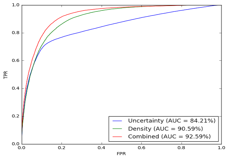
(a) MNIST dataset.

(b) SVHN dataset.

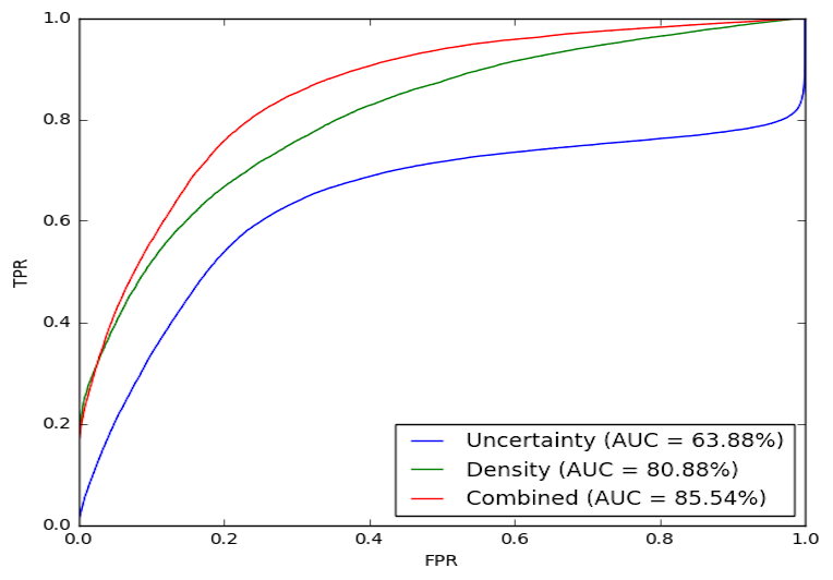
(c) CIFAR-10 dataset.

Figure 9: ROCS for the different classifier types. The blue line indicates uncertainty, green line density, and red line combined. The negative class consists of both normal and noisy samples.

To evaluate our adversarial detection method, we aggregate all adversarial samples of different types into a unified set, and do the same with the noisy and normal samples. For each dataset and attack, we have built three binary classifiers:

• uncertainty: this classifier simply thresholds on the uncertainty value of a sample.

• density: this classifier simply thresholds on the negative log kernel density of a sample.

• combined: this is a simple logistic regression classifier with two features as input: the uncertainty and the density estimate.

These detection models are used to distinguish adversarial samples–the positive class–from normal and noisy samples, which jointly constitue the negative class. The logistic regression model is trained by generating adversarial samples for every correctly-classified training point using each of the four adversarial attacks, and then using the uncertainty values and density estimates for the original and adversarial samples as a labeled training set. The two features are z-scored before training.

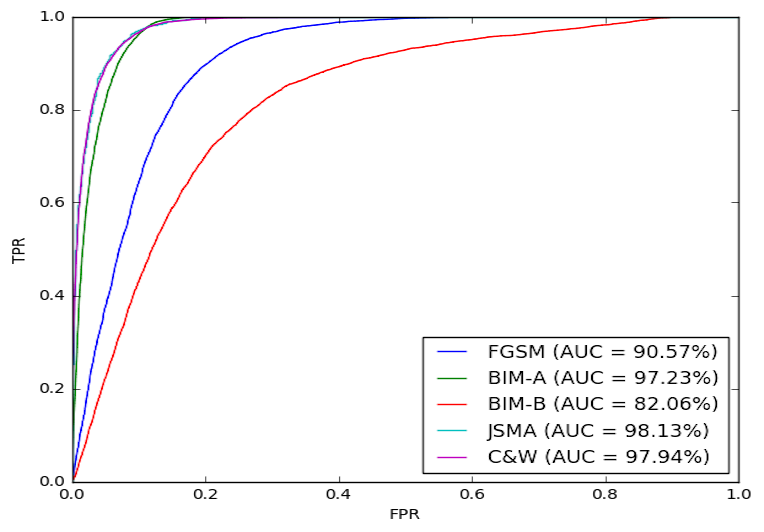
Figure 10: ROC results per adversarial attack for combined classifier on MNIST.

Because these are all threshold-based classifiers, we may generate an ROC for each method. Figure 9 shows ROCs for each classifier with a couple of datasets. We see that the performance of the combined classifier is better than either the uncertainty or density classifiers, demonstrating that each feature is able to detect different qualities of adversarial features. Further, the ROCs demonstrate that the uncertainty and density estimates are effective indicators that can be used to detect if a sample is adversarial. Figure 10 shows the ROCs for each individual attack; the combined classifier is able to most easily handle the JSMA, BIM-A and C&W attacks.

In Table 3, the ROC-AUC measures are shown, for each of the three classifiers, on each dataset, for each attack. The performance is quite good, suggesting that the combined classifier is able to effectively detect adversarial samples from a wide range of attacks on a wide range of datasets.

6 Conclusions

We have shown that adversarial samples crafted to fool DNNs can be effectively detected with two new features: kernel density estimates in the subspace of the last hidden layer, and Bayesian neural network uncertainty estimates. These two features handle complementary situations, and can be combined as an effective defense mechanism against adversarial samples. Our results report that we can, in some cases, obtain an ROC-AUC for an adversarial sample detector of up to 90% or more when both normal and noisy samples constitute the negative class. The performance is good on a wide variety of attacks and a range of image datasets.

In our work here, we have only considered convolutional neural networks. However, we believe that this approach can be extended to other neural network architectures as well. Gal (2015) showed that the idea of dropout as a Bayesian approximation could be applied to RNNs as well, allowing for robust uncertainty estimation. In future work, we aim to apply our features to RNNs and other network architectures.

References

- Bengio et al. (2013) Bengio, Y., Mesnil, G., Dauphin, Y., and Rifai, S. Better mixing via deep representations. In Proceedings of the 30th International Conference on International Conference on Machine Learning (ICML ’13), pp. 552–560, 2013.
- Carlini & Wagner (2016) Carlini, N. and Wagner, D. Towards evaluating the robustness of neural networks. arXiv:1608.04644, 2016.
- Fawzi et al. (2016) Fawzi, A., Moosavi-Dezfooli, S., and Frossard, P. Robustness of classifiers: from adversarial to random noise. In Advances in Neural Information Processing Systems 29 (NIPS 2016), pp. 1632–1640, 2016.
- Gal (2015) Gal, Y. A theoretically grounded application of dropout in recurrent neural networks. In Advances in Neural Information Processing Systems 29 (NIPS 2016), pp. 1019–1027, 2015.
- Gal & Ghahramani (2015) Gal, Y. and Ghahramani, Z. Dropout as a Bayesian approximation: representing model uncertainty in deep learning. In Proceedings of The 33rd International Conference on Machine Learning (ICML ’16), pp. 1050–1059, 2015.
- Gardner et al. (2015) Gardner, J.R., Upchurch, P., Kusner, M.J., Li, Y., Weinberger, K.Q., Bala, K., and Hopcroft, J.E. Deep manifold traversal: changing labels with convolutional features. arXiv preprint arXiv:1511.06421, 2015.
- Goodfellow et al. (2015) Goodfellow, I.J., Shlens, J., and Szegedy, C. Explaining and harnessing adversarial examples. International Conference on Learning Representations, 2015.
- Jones et al. (1996) Jones, M.C., Marron, J.S., and Sheather, S.J. A brief survey of bandwidth selection for density estimation. Journal of the American Statistical Association, 91(433):401–407, 1996.
- Kurakin et al. (2017) Kurakin, A., Goodfellow, I.J., and Bengio, S. Adversarial examples in the physical world. International Conference on Learning Representations, 2017.
- LeCun et al. (1989) LeCun, Y., Boser, B., Denker, J.S., Henderson, D., Howard, R.E., Hubbard, W., and Jackel, L.D. Backpropagation applied to handwritten zip code recognition. Neural computation, 1(4):541–551, 1989.
- LeCun et al. (2015) LeCun, Y., Bengio, Y., and Hinton, G. Deep learning. Nature, 521:436–444, 2015.
- Lee & Verleysen (2007) Lee, J.A. and Verleysen, M. Nonlinear Dimensionality Reduction. Springer Science+Business Media, LLC, New York, NY, USA, 2007.
- Metzen et al. (2017) Metzen, J.H., Genewein, T., Fischer, V., and Bischoff, B. On detecting adversarial perturbations. International Conference on Learning Representations, 2017.
- Papernot et al. (2016a) Papernot, N., Goodfellow, I.J., Sheatsley, R., Feinman, R., and McDaniel, P. cleverhans v1.0.0: an adversarial machine learning library. arXiv preprint arXiv:1610.00768v3, 2016a.
- Papernot et al. (2016b) Papernot, N., McDaniel, P., Jha, S., Fredrikson, M., Celik, Z.B., and Swami, A. The limitations of deep learning in adversarial settings. In Proceedings of the 1st IEEE European Symposium on Security and Privacy, pp. 372–387, 2016b.
- Papernot et al. (2016c) Papernot, N., McDaniel, P., Wu, X., Jha, S., and Swami, A. Distillation as a defense to adversarial perturbations against deep neural networks. Symposium on Security and Privacy, pp. 582–597, 2016c.
- Rasmussen & Williams (2005) Rasmussen, C.E. and Williams, C.K.I. Gaussian Processes for Machine Learning (Adaptive Computation and Machine Learning). The MIT Press, 2005. ISBN 026218253X.
- Srivastava et al. (2014) Srivastava, N., Hinton, G.E., Krizhevsky, A., Sutskever, I., and Salakhutdinov, R. Dropout: a simple way to prevent neural networks from overfitting. Journal of Machine Learning Research, 15:1929–1958, 2014.
- Szegedy et al. (2014) Szegedy, C., Zaremba, W., and Sutskever, I. Intriguing properties of neural networks. International Conference on Learning Representations, 2014.
- Tanay & Griffin (2016) Tanay, T. and Griffin, L. A boundary tilting perspective on the phenomenon of adversarial samples. arXiv preprint arXiv:1608.07690, 2016.