Open source Matrix Product States: Opening ways to simulate entangled many-body quantum systems in one dimension

Abstract

Numerical simulations are a powerful tool to study quantum systems beyond exactly solvable systems lacking an analytic expression. For one-dimensional entangled quantum systems, tensor network methods, amongst them Matrix Product States (MPSs), have attracted interest from different fields of quantum physics ranging from solid state systems to quantum simulators and quantum computing. Our open source MPS code provides the community with a toolset to analyze the statics and dynamics of one-dimensional quantum systems. Here, we present our open source library, Open Source Matrix Product States (OSMPS), of MPS methods implemented in Python and Fortran2003. The library includes tools for ground state calculation and excited states via the variational ansatz. We also support ground states for infinite systems with translational invariance. Dynamics are simulated with different algorithms, including three algorithms with support for long-range interactions. Convenient features include built-in support for fermionic systems and number conservation with rotational $\mathcal{U}(1)$ and discrete $\mathbb{Z}_{2}$ symmetries for finite systems, as well as data parallelism with MPI. We explain the principles and techniques used in this library along with examples of how to efficiently use the general interfaces to analyze the Ising and Bose-Hubbard models. This description includes the preparation of simulations as well as dispatching and post-processing of them.

PROGRAM SUMMARY

Program title: Open Source Matrix Product States (OSMPS), v2.0
Program summary and documentation: http://openmps.sourceforge.io/
Program obtainable from: http://sourceforge.net/p/openmps
Licensing provisions: GNU GPL v3 (Minor parts follow the copyright of the Expokit package.)
Programming language: Python, Fortran2003, MPI for parallel computing
Compilers (Fortran): gfortran, ifort, g95
Operating system: Linux, Mac OS X, Windows
Supplementary material: We provide programs to reproduce selected figures in the Appendices.
Nature of the problem: Solving the ground state and dynamics of a many-body entangled quantum system is a challenging problem; the Hilbert space grows exponentially with system size. Complete diagonalization of the Hilbert space to floating point precision is limited to less than forty qubits.
Solution method: Matrix Product States in one spatial dimension overcome the exponentially growing Hilbert space by truncating the least important parts of it. The error can be well controlled. Local neighboring sites are variationally optimized in order to minimize the energy of the complete system. We can target the ground state and low lying excited states. Moreover, we offer various methods to solve the time evolution following the many-body Schrödinger equation. These methods include e.g. the Suzuki-Trotter decompositions using local propagators or the Krylov method, both approximating the propagator on the complete Hilbert space.

1 Introduction

Numerical methods have been widely used to study physical systems in quantum mechanics that are not exactly solvable. In many-body systems we encounter with the exponentially growing Hilbert space a challenge to develop methods which can still simulate quantum systems on a classical computer. Starting with the Density Matrix Renormalization Group (DMRG)  [1, 2], a wide range of tensor network methods have been developed. Especially in one dimension, where numerical scaling and conditioning are best, such methods offer strong alternatives to other methods such as Quantum Monte Carlo [3, 4] and the Truncated Wigner approximation [5, 6]. Applications include solid state systems, ultracold atoms and molecules, Rydberg atoms, quantum information and quantum computing, and Josephson junction-based superconducting electro-mechanical nano devices. Matrix Product States (MPSs) [7, 8, 9, 10] define the tensor network at the foundation of the DMRG method. MPSs themselves represent a pure quantum state constructed on local Hilbert spaces of lattice sites or discretized systems. They handle the exponentially growing Hilbert space by limiting the entanglement between any two parts of the system. Numerical methods using MPSs support static results such as ground states and time evolution of pure states. In principle, highly entangled states can be represented as MPSs, but due to the upper bound of entanglement set as a parameter, they are only accurate as long as the entanglement does not exceed this bound guaranteeing feasible computation times. This point is addressed in the main part of this paper in detail. Moreover, MPSs can exploit intrinsic characteristics of the systems such as symmetries [11, 12]. Beyond MPSs, tensor network methods are extended for multiple purposes such as 2D systems via Projected Entangled Pair States (PEPS) [13], tree tensor networks (TTNs) [14], open systems with quantum trajectories (QT) [15, 16] or Matrix Product Density Operators (MPDOs) [17, 18]. Although there have been many developments in many-body quantum simulation over the last ten to twenty years [19], from multi-scale entanglement renormalization ansatz (MERA) [20] to minimally entangled typical thermal states (METTS) [21] to dynamical mean-field theory [22] to time-dependent density functional theory (TDDFT) [23, 24], MPS methods are the most often used and well-established for strongly correlated quantum systems and appropriate for large-scale open source development. The impact of these methods is represented by the large number of open source packages for MPS and DMRG [25, 26, 27, 28, 29, 30, 31, 32, 33, 34, 35, 36, 37, 38, 39], not counting proprietary efforts of multiple other groups.

We present in this paper our open source Matrix Product State (OSMPS) library, which is available on SourceForge [40]. We have over 2300 downloads since its initial release in January 2014. The library or a derivative of the library has been used in various publications [41, 42, 43, 44, 45, 46, 47, 48, 49, 50, 51, 52, 53, 54, 55, 56]. Our implementations cover features such as variational ground and excited state searches and real time evolution for finite systems as well as ground states of infinite systems [57]. We provide built-in features such as support for symmetries, e.g. rotational $\mathcal{U}(1)$ symmetry used for number conservation in the Bose-Hubbard model and discrete $\mathbb{Z}_{2}$ symmetry occurring in the quantum Ising model, and present them in the case studies of this article. These symmetries lead to a speedup in terms of computation time and allow us to address specific states. Our libraries also support data parallel execution via Message Passing Interface (MPI) to utilize modern high performance computing resources efficiently. We illustrate the algorithms in our library together with examples of models.

One motivation for the development of OSMPS is our focus on ultracold molecules and other quantum simulator architectures incorporating long-range interacting synthetic quantum matter. Where some MPS-based algorithms are limited to nearest neighbor terms in one-dimensional systems, molecules and many other systems have long-range interactions, e.g. due to dipolar effects. In order to treat such systems, many of the algorithms in OSMPS, including dynamics algorithms, feature support for long-range interactions.

This paper is intended for two audiences: First, tensor network methods and our interfaces are introduced for researchers not familiar with such methods, but in need of numerical simulations of correlations, entanglement, and dynamics in many-body systems. On the other hand, experienced researchers within the tensor networks community should have a clear way to understand the concrete and useful details of our implementations. The paper is organized as follows. In Sec. 2, we introduce the general idea of tensor networks, and provide in addition appropriate references for further reading. We continue with the example of the Ising model in Sec. 3 to demonstrate the variational ground state search including the general setup of systems and then highlight the other algorithms in the following sections. Section 4 describes the variational search for excited states and the infinite MPS (iMPS) for the thermodynamic limit. The time evolution methods including Krylov, Time-Evolving Block Decimation (TEBD), Time-Dependent Variational Principle (TDVP), and local Runge-Kutta follow in Sec. 5. We describe future developments ahead of the conclusion in Sec. 7. The appendices cover topics such as convergence studies for the algorithms, convenient features, and technical information for installation and the scope of the open source project.

2 Basic concepts in tensor network techniques

In this section, we briefly review the concepts of tensor network techniques. Readers familiar with MPS algorithms can continue on to Sec. 3 discussing the design of simulations specifically for OSMPS. The MPS algorithms rely heavily on the Schmidt decomposition of a quantum system, which can be explained best in the case of two subsystems $1$ and $2$ and their wave function $\left|{\psi_{1,2}}\right\rangle$. Each subsystem is defined on a local Hilbert space $\mathcal{H}_{k}$ of dimension $d_{k}$, and is spanned by an orthonormal basis of states $\{|i_{k}\rangle\}$. The joint Hilbert space of subsystem $1$ and $2$ is formed via the tensor product $\mathcal{H}=\mathcal{H}_{1,2}=\mathcal{H}_{1}\otimes\mathcal{H}_{2}$ and has a dimension $d_{1}\times d_{2}$. The Schmidt decomposition is then based on a set of local wave functions $\left|{\psi^{[1]}_{\alpha}}\right\rangle$ and $\left|{\psi^{[2]}_{\alpha}}\right\rangle$

$$|\psi_{1,2}\rangle=\sum_{\alpha=1}^{\chi_{\max}}\lambda_{\alpha}|\psi^{[1]}_{\alpha}\rangle|\psi^{[2]}_{\alpha}\rangle\,.$$ (1)

The Schmidt decomposition corresponds to a singular value decomposition (SVD) where the singular values are the $\lambda_{\alpha}$. The number of non-zero singular values serves as a coarse measure of entanglement between the systems 1 and 2, known as the Schmidt number or Schmidt rank. We dub the maximal number of singular values as $\chi_{\max}$. Tracing out over either of the subsystems, we obtain the reduced density matrix of the other subsystem. This demonstrates that the eigenvalues of the reduced density matrices $\rho_{1}=\mathrm{Tr}_{2}|\psi_{1,2}\rangle\langle\psi_{1,2}|$ and $\rho_{2}=\mathrm{Tr}_{1}|\psi_{1,2}\rangle\langle\psi_{1,2}|$ are $\{\lambda_{\alpha}^{2}\}$ [58].

The Schmidt decomposition is unique up to rotations within subspaces of degenerate singular values for a chosen basis. Local unitary transformations such as basis transformations affecting each half of the bipartition separately are possible in general, because they do not change the entanglement, i.e., the number and value of non-zero singular values. MPSs generalize the Schmidt decomposition by allowing for rotations within the Schmidt bases $|\psi^{[k]}_{\alpha}\rangle$ that keep the amount of bipartite entanglement between the two subsystems fixed:

$$|\psi_{1,2}\rangle=\sum_{\alpha=1}^{\chi_{\max}}\sum_{i_{1}=1}^{d_{1}}\sum_{i_{2}=1}^{d_{2}}A_{\alpha}^{[1]i_{1}}A_{\alpha}^{[2]i_{2}}\left|{i_{1}}\right\rangle\left|{i_{2}}\right\rangle\,.$$ (2)

In addition, while the Schmidt decomposition is only defined for a bipartite system, the MPS form can be extended to any number of degrees of freedom.

We take the example of a two-site system to illustrate the connection between the Schmidt and MPS decompositions. Subsystem $1$ is the site with $k=1$ and subsystem two corresponds to the site with $k=2$. The MPS decomposition of such a system is described in Eq. (2). We rewrite any state $\left|{\psi_{\alpha}}\right\rangle$ in Eq. (1) as a matrix of complex numbers $c_{i_{1}i_{2}}$ and its corresponding basis states, that is $\sum_{i_{1}i_{2}}c_{i_{1}i_{2}}|i_{1}\rangle|i_{2}\rangle$. In Eq. (1), each dimension $k$ is spanned by $\chi_{\max}$ orthonormal vectors. We can rewrite the sets of these vectors as matrices (rank-two tensors), where each column of the matrix represents a vector in the case of site $1$, and each row is filled with one vector for site $2$. Then, the matrix $A^{[k]}$ in Eq. (2) represents a rank-2 tensor for site $k$ and the singular values are contained in either $A^{[k]}$. A single element of the matrix $A^{[k]}$ can be written as $A_{\alpha}^{[k]j_{k}}=\left\langle j_{k}\middle|\psi_{\alpha}^{[k]}\right\rangle$ in the two-site case above. Thus, the indices of the tensors $A^{[k]}$ correspond to the local Hilbert space $i_{k}$ and the singular values of the Schmidt decomposition $\alpha$. Throughout the paper we note the site index of a tensor in brackets, i.e., the $k$ in $A^{[k]}$.

\begin{overpic}[width=238.49231pt,unit=1mm]{./picts/MPS_HighRes.pdf} \put(5.0,-6.0){\color[rgb]{0,0,1}$A_{\alpha_{1}}^{[1]i_{1}}$} \put(35.0,2.0){\color[rgb]{0,0,1}$A_{\alpha_{1},\alpha_{2}}^{[2]i_{2}}$} \put(58.0,8.0){\color[rgb]{0,0,1}$A_{\alpha_{2},\alpha_{3}}^{[3]i_{3}}$} \put(78.0,14.0){\color[rgb]{0,0,1}$A_{\alpha_{3},\alpha_{4}}^{[4]i_{4}}$} \put(95.0,20.0){\color[rgb]{0,0,1}$A_{\alpha_{4}}^{[5]i_{5}}$} \put(3.0,27.0){\color[rgb]{0,0.390625,0}$i_{1}$} \put(33.0,31.0){\color[rgb]{0,0.390625,0}$i_{2}$} \put(55.0,35.0){\color[rgb]{0,0.390625,0}$i_{3}$} \put(73.0,38.0){\color[rgb]{0,0.390625,0}$i_{4}$} \put(87.0,39.0){\color[rgb]{0,0.390625,0}$i_{5}$} \put(24.0,8.0){\color[rgb]{1,0,0}$\alpha_{1}$} \put(49.0,14.0){\color[rgb]{1,0,0}$\alpha_{2}$} \put(70.0,19.0){\color[rgb]{1,0,0}$\alpha_{3}$} \put(85.0,21.5){\color[rgb]{1,0,0}$\alpha_{4}$} \end{overpic}

Figure 1: Tensor network representation of an MPS of five sites for open boundary conditions. The state is decomposed into local tensors representing each site. These tensors are connected to their nearest neighbors via the Schmidt decomposition where singular values are truncated to maintain feasible run times for larger systems. The indices for the local Hilbert space $i_{k}$ are connected for measurements, e.g. for the norm $\langle\psi|\psi\rangle$, with their complex conjugated counterpart.

In order to generalize this decomposition for a system with $L$ sites, successive SVDs lead to one tensor per site where the tensors are now rank-2 at the boundaries and rank-3 in the bulk of the system, as shown in the representation as a tensor network in Fig. 1:

$$|\psi_{1,\ldots,L}\rangle=\sum_{\alpha_{1}\cdots\alpha_{L-1}}\sum_{i_{1}\cdots i_{L}}A_{\alpha_{1}}^{[1]i_{1}}A_{\alpha_{1},\alpha_{2}}^{[2]i_{2}}\cdots A_{\alpha_{L-2},\alpha_{L-1}}^{[L-1]i_{L-1}}A_{\alpha_{L-1}}^{[L]i_{L}}\left|{i_{1}}\right\rangle\cdots\left|{i_{L}}\right\rangle\,.$$ (3)

If we allow the indices $\alpha_{j}$ to run over exponentially large values $\sim d^{L/2}$ ($d=d_{k}$ the local dimension, assumed uniform for simplicity), such a representation is exact, but manipulating this exact representation also scales exponentially with the system size and we do not gain anything over exact diagonalization methods.

We now introduce the key approximation in the MPS algorithm, that is the truncation of the Hilbert space according to the singular values from the Schmidt decomposition. The essential idea here is to replace the number of singular values $\chi_{\max}$ with a reduced number $\chi$: for instance, if there are singular values less than $10^{-16}$ there is no reason to count them toward the amount of entanglement between the two subsystems. Thus $\chi$ becomes the reduced Schmidt rank, the major convergence parameter of the whole MPS algorithm, as we will show. We obtain these singular values for any splitting in two connected subsystems, and the truncation is encoded in the maximum range of the auxiliary indices $\alpha_{i}$. Considering an approximated state $\left|{\psi^{\prime}}\right\rangle$ truncated to the first $\chi$ singular values at some particular bond of the normalized state $\left|{\psi}\right\rangle$ with $\chi_{\max}$ singular values at that bond, the overlap between the two states is

$$\left\langle\psi^{\prime}\middle|\psi\right\rangle = \frac{\sum_{i=1}^{\chi}\lambda_{i}^{2}}{\sqrt{\sum_{i=1}^{\chi}\lambda_{i}^{2}}}=\sqrt{\sum_{i=1}^{\chi}\lambda_{i}^{2}}\,.$$ (4)

We prefer the overlap instead of the 2-norm of the overlap since it allows us to relate our result to the quantum fidelity in our case of pure states with real overlaps as $\mathcal{F}=\langle\psi\left|{\psi^{\prime}}\right\rangle$. We define the truncation error made in this step as $\epsilon_{\mathrm{local}}=1-\langle\psi\left|{\psi^{\prime}}\right\rangle$ and obtain

$$\epsilon_{\mathrm{local}} = 1-\sqrt{\sum_{i=1}^{\chi}\lambda_{i}^{2}}\leq\sum_{i=\chi+1}^{\chi_{\max}}\lambda_{i}^{2}\,.$$ (5)

This upper bound is useful since it relates directly to the truncated singular values. Such a truncation corresponds to a truncation of entanglement through two entanglement measures: the Schmidt rank $\chi$ and the von Neumann entropy $S$. The former is simply the number of non-zero singular values, and is an entanglement monotone. The von Neumann entropy, or bond entropy, $S$ is given as

$$S=-\sum_{i=1}^{\chi}\lambda_{i}^{2}\log(\lambda_{i}^{2})\,.$$ (6)

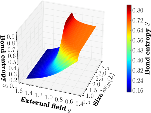
Figure 2: The compression of the quantum state in the MPS acts on the singular values of the Schmidt decomposition in Eq. (1). The bond entropy or von Neumann entropy at the center bond for the nearest-neighbor quantum Ising model $H=-J\sum\sigma_{k}^{z}\sigma_{k+1}^{z}-Jg\sum\sigma_{k}^{x}$, defined later in Eq. (15), peaks around the critical point for increasing system sizes.

In Fig. 2 we show the bond entropy for the bipartition at the center bond for the quantum Ising model with transverse field as a function of the system size and external field. Errors in the MPS approach originate in high entanglement; therefore, simulations for increasing system sizes and around the quantum critical point are more vulnerable to smaller cutoffs $\chi$. The quantum critical point for the Ising model is $h_{c}=1.0$ and becomes visible as a red ridge in Fig. 2 for large system sizes. The ground state of the ferromagnetic phase in the limit of zero external field, also called the Greenberger-Horne-Zeilinger (GHZ) state, is the superposition of all spins up and all spins down, i.e. $\left(|\uparrow\cdots\uparrow\rangle+|\downarrow\cdots\downarrow\rangle\right)/\sqrt{2}$. We expect an entropy of $S=-\log(0.5)\approx 0.69$, which agrees well with the results in the Fig. 2. For gapped 1D systems with short-range interactions, the so-called area law for entanglement [59] states that the entanglement at any bipartition is independent of the length of the subsystems (and hence of the system size $L$). Since the bond entropy is an entanglement measure, this upper bound can be used as the gap opens away from the critical point. At the critical point, the entanglement grows logarithmically with the subsystem size.

We introduce a list of basic operations that can be performed on tensor networks, and explain the orthogonality center, an isometrization or gauge, used in the OSMPS algorithms. For these linear algebra operations on tensors, we suppress the basis kets of the quantum states for simplicity throughout the paper. One key feature of every MPS with open boundary conditions is that introducing an orthogonality center leads to faster local measurements and error reduction in the truncation [60]. We introduce the left and right canonical form of tensors according to

$$A_{\alpha_{k-1},\alpha_{k}}^{[k]i_{k}}=L_{\alpha_{k-1},\alpha_{k}}^{[k]i_{k}}\;\;\mathrm{if}\;\;\begin{cases}A^{[j]}=L^{[j]}\;\forall\;j<k\\ \mathrm{and\leavevmode\nobreak\ }\sum_{\alpha_{k-1},i_{k}}A_{\alpha_{k-1},\alpha_{k}}^{[k]i_{k}}(A_{\alpha_{k-1},\alpha_{k}^{\prime}}^{[k]i_{k}})^{\ast}=\mathbb{I}_{\alpha_{k},\alpha_{k}^{\prime}}\,,\end{cases}$$

$$A_{\alpha_{k-1},\alpha_{k}}^{[k]i_{k}}=R_{\alpha_{k-1},\alpha_{k}}^{[k]i_{k}}\;\;\mathrm{if}\;\;\begin{cases}A^{[j]}=R^{[j]}\;\forall\;j>k\\ \mathrm{and\leavevmode\nobreak\ }\sum_{\alpha_{k},i_{k}}A_{\alpha_{k-1},\alpha_{k}}^{[k]i_{k}}(A_{\alpha_{k-1}^{\prime},\alpha_{k}}^{[k]i_{k}})^{\ast}=\mathbb{I}_{\alpha_{k-1},\alpha_{k-1}^{\prime}}\,.\end{cases}$$ (7)

The left (right) canonical forms $L^{[k]}$ $\left(R^{[k]}\right)$ are unitary matrices, e.g. from the SVD obtained from the Schmidt decomposition in Eq. (1). These conditions apply if the singular values have not been multiplied into the tensor. We define the orthogonality center as the site which has only left orthogonal tensors on the left side and right orthogonal tensor on the right side. This feature becomes beneficial for measurements as the contractions in the condition of Eq. (7) do not have to be calculated knowing that the result is the identity $\mathbb{I}$. Stated equivalently, the tensor of the orthogonality center $A^{[k]i_{k}}_{\alpha\beta}$ consists of the coefficients of the wave function in the orthonormal basis spanned by the local states $|i_{k}\rangle$ and the left and right Schmidt vectors given by products of the other MPS tensors. With these definitions, we can derive the overlap from Eq. (4). We assume that we truncate singular values at the bond of the sites $k$ and $k+1$ and the sites up to and including site $k$ are of the form $L^{[j\leq k]}$ and the tensors beginning on site $k+1$ are of type $R^{[j\geq k+1]}$. The truncation does not affect any of the tensors $L^{[j\leq k]}$ or $R^{[j\geq k+1]}$. Contracting these tensors for the overlap with their complex conjugated counterparts, we obtain identities on all sites and $\left\langle\psi^{\prime\prime}\middle|\psi\right\rangle$ simplifies to

$$\left\langle\psi^{\prime}\middle|\psi\right\rangle = \sum_{\alpha_{k-1},\alpha_{k}}\lambda_{\alpha_{k-1},\alpha_{k}}\lambda_{\alpha_{k-1},\alpha_{k}}^{\prime}\,,$$ (8)

where $\left|{\psi^{\prime\prime}}\right\rangle$ is the unnormalized truncated state and $\left|{\psi^{\prime}}\right\rangle$ the truncated normalized state. The diagonal structure of the matrices $\lambda$ containing the singular values leads to $\left\langle\psi^{\prime}\middle|\psi\right\rangle=\sum_{\alpha}\lambda_{\alpha}\lambda_{\alpha}^{\prime}$. Since the smallest singular values in $\lambda^{\prime}$ are set to zero, the result is the sum of the squared singular values in $\lambda^{\prime}$. The additional term in the denominator in Eq. (4) originates in the normalization of $\left|{\psi^{\prime\prime}}\right\rangle$. We emphasize that this procedure only works if the sites are completely in the form of $L^{[j\leq k]}$ and $R^{[j\geq k+1]}$ since otherwise, the contraction with the complex conjugated tensor does not lead to an identity.

Moreover, we introduce the following actions on tensors in our MPS library:

• Contractions over two tensors are defined as the summation over one (or more) common indices, and hence generalize matrix-matrix multiplication to higher-rank tensors. A commonly used example would be to contract two neighboring tensors of an MPS, $A_{\alpha_{k-1},\alpha_{k}}^{[k]i_{k}}$ and $A_{\alpha_{k},\alpha_{k+1}}^{[k+1]i_{k+1}}$, to one tensor representing the sites $k$ and $k+1$. The summation is in this case over the index $\alpha_{k}$ and we obtain a tensor $\Theta_{\alpha_{k-1},\alpha_{k+1}}^{[k,k+1]i_{k},i_{k+1}}$.

• Splitting of a tensor is the reverse action of a contraction. The indices of the tensor form two subgroups where the splitting is enacted between those two groups. Taking the two site tensor $\Theta_{\alpha_{k-1},\alpha_{k+1}}^{[k,k+1]i_{k},i_{k+1}}$ as an example, we group $\alpha_{k-1},i_{k}$ together and $i_{k+1},\alpha_{k+1}$ in order to obtain two single site tensors, up to a possible truncation. The splitting can be achieved via three possibilities:

  • An SVD splits the tensor directly into two unitary tensors and the singular values, described by

    $$\Theta_{\alpha_{k-1},\alpha_{k+1}}^{[k,k+1]i_{k},i_{k+1}} = L_{\alpha_{k-1},\alpha_{k}}^{[k]i_{k}}\lambda_{\alpha_{k}}R_{\alpha_{k},\alpha_{k+1}}^{[k+1]i_{k+1}}\,,$$ (9)

    where the singular values $\lambda_{\alpha_{k}}$ allow us to truncate the state to a certain $\chi$. The maximal bond dimension is defined as $\min\left(\chi_{k-1}d_{k},d_{k+1}\chi_{k+1}\right)$.

  • The eigenvalue decomposition is related to the singular value decomposition, which is the reason the eigenvalue decomposition can replace the SVD. If the SVD decomposes $A$ into $U\lambda V$, the eigendecomposition $\mathcal{E}(\;\cdot\;)$ is set up as follows:

    $$\mathcal{E}(AA^{\dagger})=\mathcal{E}\left(U\lambda VV^{\dagger}\lambda U^{\dagger}\right)=\mathcal{E}\left(U\lambda^{2}U^{\dagger}\right)=U\lambda^{2}U^{\dagger}\,.$$ (10)

    The eigendecomposition of $AA^{\dagger}$, which is built from a matrix-matrix multiplication, returns a unitary matrix and the singular values squared. To obtain the right matrix, we multiply $U^{\dagger}$ with the original matrix $A$ leading to

    $$U^{\dagger}A=U^{\dagger}U\lambda V=\lambda V\,,$$ (11)

    which already contains the singular values. After completing the series of steps, we obtain

    $$\Theta_{\alpha_{k-1},\alpha_{k+1}}^{[k,k+1]i_{k},i_{k+1}} = L_{\alpha_{k-1},\alpha_{k}}^{[k]i_{k}}A_{\alpha_{k},\alpha_{k+1}}^{[k+1]i_{k+1}}\,,$$ (12)

    where the truncation is possible due to the knowledge of $\lambda^{2}$ in the intermediate step of Eq. (10), although the singular values do not appear in the previous equation (12). As in the case of the SVD, the maximal bond dimension is $\min(\chi_{k-1}d_{k},d_{k+1}\chi_{k+1})$. The unitary matrix can be obtained for the right side starting with $A^{\dagger}A$. This procedure is generally faster than the SVD.

  • The QR decomposition decomposes a matrix into a unitary matrix and an upper triangular matrix $T$. If the unitary matrix is on the right side, it may be referred to as RQ decomposition. It does not allow for truncation as the singular values are not calculated. The example for the QR is

    $$\Theta_{\alpha_{k-1},\alpha_{k+1}}^{[k,k+1]i_{k},i_{k+1}} = L_{\alpha_{k-1},\alpha_{k}}^{[k]i_{k}}T_{\alpha_{k},\alpha_{k+1}}^{[k+1]i_{k+1}}\,.$$ (13)

    Therefore, the new bond dimension is the maximal one, $\chi=\chi_{\mathrm{max}}=\min(\chi_{k-1}d_{k},$ $d_{k+1}\chi_{k+1})$. The fact that the QR scenario is not rank revealing is the reason for not using it in the splitting of two sites in the library, but it is used for shifting as explained in the following.

  The different options for splitting a tensor are summarized in Fig. 3. We choose the SVD to obtain the singular values and two unitary matrices. In contrast, the eigenvalue decomposition yields a unitary matrix and the singular values. The QR decomposition differs from the first two methods as it does not reveal the singular values and returns only one unitary matrix. Therefore, the QR is computationally less expensive than the approach with the eigenvalue decomposition. The SVD is computationally more costly than both other algorithms.

  \begin{overpic}[width=325.215pt,unit=1mm]{./picts/Splitting.pdf} \put(7.0,20.0){$L^{[k]}$} \put(13.0,19.0){$\lambda$} \put(10.0,4.0){$\chi\leq\chi_{\max}$} \put(19.0,20.0){$R^{[k+1]}$} \put(21.0,32.0){{\color[rgb]{1,0,0}SVD}} \put(44.0,20.0){$L^{[k]}$} \put(47.0,4.0){$\chi\leq\chi_{\max}$} \put(54.0,20.0){$A^{[k+1]}$} \put(46.0,32.0){{\color[rgb]{1,0,0}$\mathcal{E}$}} \put(79.0,20.0){$L^{[k]}$} \put(83.0,4.0){$\chi_{\max}$} \put(90.0,20.0){$A^{[k+1]}$} \put(73.0,32.0){{\color[rgb]{1,0,0}QR}} \put(30.0,47.0){$\alpha_{k-1}$} \put(44.0,37.0){$i_{k}$} \put(47.0,53.0){$\Theta^{[k,k+1]}$} \put(54.0,37.0){$i_{k+1}$} \put(64.0,47.0){$\alpha_{k+1}$} \put(1.0,22.0){(a)} \put(38.0,22.0){(b)} \put(72.0,22.0){(c)} \end{overpic}

  Figure 3: Methods for splitting a two site tensor into two one site tensors include (a) an SVD decomposition, (b) an eigenvalue decomposition $\mathcal{E}$ in combination with matrix multiplications, and (c) a QR decomposition.

• Shifting the orthogonality center can be done with local operations, meaning that the operations act only at one site at a time and do not use any two site tensors. Running an SVD or QR (RQ) decomposition for site $k$ on a single rank-3 tensor with dimensions $\chi_{k-1}$, $d$, and $\chi_{k}$, we reshape the tensor as a $\chi_{l}d\times\chi_{r}$ ($\chi_{l}\times d\chi_{r}$) matrix and obtain a left-canonical (right-canonical) unitary tensor for site $k$ and an additional matrix. The additional matrix consists of the singular values contracted into a unitary matrix when choosing an SVD. For the QR (RQ) decomposition we obtain a left (right) canonical unitary and an additional upper triangular matrix. This additional matrix can be contracted to the corresponding neighboring site $k\pm 1$, resulting in that site becoming the new orthogonality center. We note in this case that the QR and RQ decomposition does not change the ranks of the matrices, and is roughly a factor of two faster than the SVD.

With the knowledge of the basic features of an MPS, we introduce in the next chapter how a model is defined in the OSMPS library and how we obtain results as in Fig. 2.

3 Defining systems and variational ground state search

We now outline the definition of systems in OSMPS. As an example we consider finding the ground state of the finite size quantum Ising model. The 1D long-range transverse field Ising Hamiltonian is [61, 62]

$$H = -J\sum_{i<j\leq L}\frac{\sigma_{i}^{z}\sigma_{j}^{z}}{(j-i)^{\alpha}}-Jg\sum_{i=1}^{L}\sigma_{i}^{x}\,,$$ (14)

where the operators are defined over the Pauli matrices $\left\{\sigma_{i}^{x},\sigma_{i}^{y},\sigma_{i}^{z}\right\}$ acting on a site $i$ in the system. The interactions between the spins at different sites decay following a power-law introduced in the first term of the Hamiltonian governed by $\alpha$, the distance $|j-i|$, and the overall energy scale $J$. The external field is governed by the dimensionless $g$ appearing in the second term of the Hamiltonian. The number of sites is $L$. We focus in this section on the nearest neighbor case $H_{\mathrm{NN}}$ obtained for the limit $\alpha{}\rightarrow{}\infty{}$, commonly called the transverse quantum Ising model,

$$H_{\mathrm{NN}}=-J\sum_{i=1}^{L-1}\sigma_{i}^{z}\sigma_{i+1}^{z}-Jg\sum_{i=1}^{L}\sigma_{i}^{x}\,.$$ (15)

The overall approach to OSMPS is a user-friendly Python environment calling a Fortran core for the actual calculations. This scheme is depicted in Fig. 4. Thus, we guide the reader through the simulation with a corresponding summary of the Python files; the complete files are contained in supplemental material, see Appendix H.

\begin{overpic}[width=433.62pt,unit=1mm]{./picts/Workflow_1.pdf} \put(2.0,78.0){(a)} \put(15.0,45.0){{\Large\color[rgb]{1,0,0} Python}} \end{overpic}

\begin{overpic}[width=433.62pt,unit=1mm]{./picts/Workflow_2.pdf} \put(8.0,77.0){(b)} \put(28.0,45.0){{\Large\color[rgb]{1,0,0} Fortran}} \end{overpic}

\begin{overpic}[width=433.62pt,unit=1mm]{./picts/Workflow_3.pdf} \put(2.0,78.0){(c)} \put(15.0,45.0){{\Large\color[rgb]{1,0,0} Python}} \end{overpic}

Figure 4: OSMPS flow chart for a simulation. The OSMPS library combines a user-friendly interface in Python with a computationally powerful core written in Fortran. (a) The simulation setup is done in Python. (b) A write function provides the files for Fortran and a corresponding read function imports the results from Fortran to Python (blue arrows). (c) The Python front end then takes care of the evaluation of the data. The plot in the flow charts shows the critical value of the external field in the Ising model as a function of the system size $L$ evaluated via the maximum of the bond entropy. Finite size scaling (FSS) delivers the critical field in the thermodynamic limit for $L\rightarrow\infty$.

From a quantum mechanical point of view the following steps are necessary to describe a system. First, we have to generate the operators which are acting on the local Hilbert space, described in Sec. 3.1. Once we have the operators, we build the Hamiltonian out of rule sets in Sec. 3.2. Then, we set up the measurements to be carried out in Sec. 3.3. This procedure completes the definition of the quantum system, but we have two more tasks with regards to the numerics. In the fourth step we define the convergence parameters of the algorithm, where Sec. 3.4 describes this step for the variational ground state search. Finally, the simulation is set up and executed in Sec. 3.5.

One general comment remains before starting with a detailed description of the simulation setup. Every simulation in OSMPS is represented by a Python dictionary, which contains observables and convergence parameters as well as general parameters such as the system size.

3.1 Operators

OSMPS comes with predefined sets of operators for three different physical systems to facilitate the setup of simulations. These predefined sets of operators are returned by the corresponding functions for bosonic systems such as the Bose-Hubbard model, fermionic systems including their phase operators originating from the Jordan-Wigner transformation, or spin operators. We use the last set in the example for the quantum Ising model. The corresponding function BuildSpinOperators returns the set of operators $\{\sigma^{+},\sigma^{-},S^{z},\mathbb{I}\}$. In order to obtain the Pauli operators $\sigma^{x}$ and $\sigma^{z}$ from the spin lowering and raising operators $\sigma^{\pm}$ and the spin operator $S_{z}$, we suggest following the prescription in Listing 1.

Listing 1: Defining the operators of the quantum Ising model overwriting $S^{Z}$ with $\sigma^{Z}$.

⬇

38import MPSPyLib as mps

39import numpy as np

40import sys

41import os

42import matplotlib.pyplot as plt

43from mpl_toolkits.mplot3d.axes3d import Axes3D

44from matplotlib import cm

3.2 Hamiltonians

Through these operators, stored in a dictionary-like Python class, we define the Hamiltonian and later on the observables. The Hamiltonian is described as a matrix product operator (MPO), which is effectively an MPS with rank-four tensors instead of rank-three tensors:

$$H=\sum_{i_{1},\ldots,i_{L}}\sum_{i_{1}^{\prime},\ldots,i_{L}^{\prime}}\sum_{\alpha_{1},\ldots,\alpha{L-1}}\!\!\!M_{\alpha_{1}}^{[1]i_{1}^{\prime},i_{1}}M_{\alpha_{1},\alpha_{2}}^{[2]i_{2}^{\prime},i_{2}}\cdots M_{\alpha_{L-1}}^{[L]i_{L}^{\prime},i_{L}}\left|{i_{1}^{\prime}}\right\rangle\left\langle{i_{1}}\right|\cdots\left|{i_{L}^{\prime}}\right\rangle\left\langle{i_{L}}\right|\,.$$ (16)

A key property is that an MPO acting on an MPS can be written as another MPS, generally with a larger bond dimension. The physical indices $i_{k}$ act on the physical indices of an MPS and take them to new physical indices $i_{k}^{\prime}$. The auxiliary indices $\alpha$ of the MPO are fused with the corresponding auxiliary indices in the MPS. For most physical operators, this structure of rank-4 tensors is sparse and therefore we rather seek for an efficient implementation in terms of MPO-matrices $M^{[k]}$ than in rank-4 tensors. The MPO matrix $M^{[k]}$ including the iteration over all indices for one site representing the rule sets [63, 53] for local terms, bond terms for the interaction of nearest neighbors, and exponential rules for long-range interactions between two sites takes the form

$$M^{[k]}\!\!\! = \!\!\!\begin{pmatrix}A_{\alpha_{k-1}=1,\alpha_{k}=1}^{[k]}&0&0&0\\ A_{\alpha_{k-1}=2,\alpha_{k}=1}^{[k]}&A_{\alpha_{k-1}=2,\alpha_{k}=2}^{[k]}&0&0\\ A_{\alpha_{k-1}=3,\alpha_{k}=1}^{[k]}&0&A_{\alpha_{k-1}=3,\alpha_{k}=3}^{[k]}&0\\ A_{\alpha_{k-1}=4,\alpha_{k}=1}^{[k]}&A_{\alpha_{k-1}=4,\alpha_{k}=2}^{[k]}&A_{\alpha_{k-1}=4,\alpha_{k}=3}^{[k]}&A_{\alpha_{k-1}=4,\alpha_{k}=4}^{[k]}\end{pmatrix}\,,$$ (17)

where $k=2,3,\ldots,L-1$. The matrix structure in Eq. (17) corresponds to the auxiliary indices. Each element within this structure $A_{\alpha_{k-1},\alpha_{k}}$ is a matrix acting on the local Hilbert space of site $k$, e.g. the Pauli matrix $\sigma_{k}^{z}$. Thus the auxiliary indices $\alpha$ of the rank-4 tensor encode the row and column of $M^{[k]}$, while the indices $i_{k}$ and $i_{k}^{\prime}$ are related to the local Hilbert space are located in the rows and columns of the matrices $A_{\alpha_{k-1},\alpha_{k}}$. We now illustrate the meaning of the matrices depending on their position in $M^{[k]}$. In order to build the MPO for the Hamiltonian for the long-range Ising model, we only need the first column, last row, and the diagonal of $M^{[k]}$ and store it as a sparse structure. Matrices in the first column (last row) of $M^{[k]}$ are multiplied with identity operators on the right (left) side of site $k$, i.e., they do not interact with any sites right (left) of themselves. Diagonal elements propagate operators through the system and are completed by other operators to the left and right of site $k$, and hence represent long-range interactions. For the first and last site we define the MPO-matrix as vectors

$$M^{[1]} = \begin{pmatrix}A_{1,1}^{[1]}&A_{1,2}^{[1]}&A_{1,3}^{[1]}&A_{1,4}^{[1]}\end{pmatrix}\,,\quad M^{[L]}=\begin{pmatrix}A_{1,1}^{[L]}\\ A_{2,1}^{[L]}\\ A_{3,1}^{[L]}\\ A_{4,1}^{[L]}\end{pmatrix}\,,$$ (18)

corresponding to the auxiliary rank-one structure for the MPO matrices at the boundary in Eq. (16). Note that the first MPO matrix is a row vector and the last is a column vector, resulting in the contracted MPO object Eq. (16) being a $1\times 1$ matrix in the auxiliary indices.

\begin{overpic}[width=281.85034pt,unit=1mm]{./picts/Modeling.pdf} \put(5.0,42.0){(a)} \put(25.0,42.0){(b)} \put(53.0,42.0){(c)} \put(5.0,24.0){(d)} \put(43.0,24.0){(e)} \put(73.5,27.0){{\color[rgb]{0,0,1}$f(|i-j|,\;O_{1},O_{2})$}} \put(50.0,0.0){{\color[rgb]{0,0,1}$f(|i-j|,O_{1},O_{2})$}} \put(11.0,17.5){{\color[rgb]{1,1,1}$O_{1}$}} \put(21.0,17.5){{\color[rgb]{1,1,1}$O_{2}$}} \put(31.0,17.5){{\color[rgb]{1,1,1}$O_{3}$}} \end{overpic}

Figure 5: Rules for building a Hamiltonian. (a) Local terms; (b) bond terms acting on two neighboring sites; (c) finite range terms of two operators $O_{1},O_{2}$ and a coupling depending on the distance. The coupling function $f(x)$ is a finite sum of a limited number of neighboring sites. (d) String of arbitrary operators, e.g., a three-body term built from $O_{1}$, $O_{2}$, and $O_{3}$ and (e) infinite terms of two operators $O_{1}$ and $O_{2}$ with a distance depending on decaying coupling either as a general function $f(|j-i|)$ (InfiniteFunction) or as an exponential (Exponential). Any infinite function is expressed as a sum of exponentials within OSMPS. The coupling function $f(x)$ is extended to all sites.

We now build the nearest neighbor Hamiltonian $H_{\mathrm{NN}}$ from Eq. (15) for the quantum Ising model to continue with our example. Figure 5 shows the possible rule sets provided through OSMPS. We need the local site term depicted in Fig. 5(a) and the bond term from Fig. 5(b). In general these operators are filled with identities on all other sites and act on each possible site. The corresponding MPO-matrices depending on the site index $k$ are then

$$M^{[1]} = \begin{pmatrix}-Jg\sigma_{1}^{x}&-J\sigma_{1}^{z}&\mathbb{I}\end{pmatrix}\,,\;M^{[k]}=\begin{pmatrix}\mathbb{I}&0&0\\ \sigma_{k}^{z}&0&0\\ -Jg\sigma_{k}^{x}&-J\sigma_{k}^{z}&\mathbb{I}\end{pmatrix}\,,$$

$$M^{[L]} = \begin{pmatrix}\mathbb{I}\\ \sigma_{L}^{z}\\ -Jg\sigma_{L}^{x}\end{pmatrix}\,,$$ (19)

where $k=2,3,\ldots,L-1$. To see how this MPO structure results in the proper many-body operator, we will explicitly build the Hamiltonian for three sites, i.e., $H=M^{[1]}\times M^{[2]}\times M^{[3]}$, where $\times$ is understood to be ordinary matrix multiplication in the auxiliary indices together with tensor products on the physical indices. We start by multiplying the row vector for the first site with the matrix for the second site leading to the first line of the following equation. The multiplication of this result with the column vector for the last and third site results then in the Hamiltonian

$$M^{[1]}\times M^{[2]}\times M^{[3]} = \begin{pmatrix}\left(-Jg\sigma_{1}^{x}-J\sigma_{1}^{z}\sigma_{2}^{z}-Jg\sigma_{2}^{x}\right)&-J\sigma_{2}^{z}&\mathbb{I}\end{pmatrix}\times\begin{pmatrix}\mathbb{I}\\ \sigma_{3}^{z}\\ -Jg\sigma_{3}^{x}\end{pmatrix}$$ (20)

$$= -Jg\sigma_{1}^{x}-J\sigma_{1}^{z}\sigma_{2}^{z}-Jg\sigma_{2}^{x}-J\sigma_{2}^{z}\sigma_{3}^{z}-Jg\sigma_{3}^{x}\,.$$

The MPO matrices have more entries for models beyond nearest neighbor interactions. The local terms remain in the last row of the first column as the identities stay in their places. The diagonal is set in the case of long-range interactions with an identity times a decay factor. The larger the distance between two sites becomes, the higher the contribution of the decay multiplied at each site in between. Elements in the lower triangular part of the matrix besides the first column and last row are used e.g. in the FiniteTerm rule set.

Independent of the system, we first initialize an instance of the MPO class. The different types of terms are specified via a string argument in the class function AddObservable. Keyword arguments to any MPO terms are the weight and Hamiltonian parameters hparam. Further arguments specific for the rule can be found in the documentation, e.g. the infinite function can take the function as an additional keyword argument.

Listing 2: Defining the Hamiltonian of the quantum Ising model.

⬇

49import MPSPyLib as mps

50import numpy as np

51import sys

52import os

53import matplotlib.pyplot as plt

In the code we have given a string variable name for the coupling of the bond and site term. The energy scale (J=1) and the different values for $h$ are specified later in the Python setup script inside the dictionary representing the simulation allowing for flexibility.

3.3 Observables

\begin{overpic}[width=281.85034pt,unit=1mm]{./picts/Measuring.pdf} \put(4.0,44.0){(a)} \put(15.0,44.0){(b)} \put(39.0,44.0){(c)} \put(68.0,44.0){(d)} \put(4.0,21.0){(e)} \put(22.0,21.0){(f)} \put(74.0,21.0){(g)} \end{overpic}

Figure 6: OSMPS measurements can be selected from the following options: (a) Local terms. (b) Two-site correlators including correlations for fermionic systems. (c) String operators of type $\langle O_{A}O_{B}O_{B}\ldots O_{B}O_{B}O_{C}\rangle$. (d) MPO as used in the default measurement of the energy (Hamiltonian). (e) Single site density matrices tracing over the remaining system. (f) Two-site density matrices tracing out everything but two sites as defined in Eq. (21). (g) Singular values between left and right part of the MPS.

In order to evaluate the behavior of the system, we have to define the observables. Figure 6 shows the possible measurements: local site terms including site and bond entropy, correlations, MPOs, string operators and one or two-site reduced density matrices where the reduced density matrices $\rho_{i}$ and $\rho_{i,j}$ are defined as

$$\rho_{i}=\operatorname{Tr}_{k\neq i}\left(\rho\right)\,,\qquad\rho_{i,j}=\operatorname{Tr}_{k\neq i,j}\left(\rho\right)\,,$$ (21)

where the density matrix on the complete system is defined as $\rho=\left|{\psi}\right\rangle\left\langle{\psi}\right|$. The energy as an MPO measurement of the Hamiltonian, the bond dimension, the variance within variational algorithms, or the overlap between the initial state and the time evolved state (Loschmidt echo) are measured by default. For the Ising example, we measure $\langle\sigma_{i}^{z}\rangle$ and $\langle\sigma_{i}^{z}\sigma_{j}^{z}\rangle$. Due to the local observable we gain as well the bond entropy shown in Fig. 2. The following Listing 3 shows the necessary code for measuring these observables.

Listing 3: Defining the observables of the quantum Ising model.

⬇

71import MPSPyLib as mps

72import numpy as np

73import sys

74import os

75import matplotlib.pyplot as plt

76from mpl_toolkits.mplot3d.axes3d import Axes3D

77from matplotlib import cm

78from scipy.optimize import curve_fit

3.4 Fundamentals of the library: Variational ground state search

The previous steps completed the setup of the physical system, and we continue with the specification of the convergence parameters. Therefore, we explain the variational algorithm used to find the ground state which serves as input for the algorithms for excited state search and real time evolution.

From exact diagonalization, we know how to find the ground state via solving the eigenequation, which is optimally done with sparse methods such as the Lanczos algorithm [64]. The same procedure cannot be used in the same way beyond a few tens of particles due to the exponentially growing Hilbert space in the many-body system, but the variational ground state search adapts the eigenvalue problem to an effective eigenvalue problem for a few neighboring sites. In principle, the eigenequation $H|\psi\rangle=E|\psi\rangle$ can be solved for the ground state on the complete Hilbert space using imaginary time evolution, e.g. with the Krylov method presented for the dynamics later, using the equation $\mathrm{e}^{-\beta H}$ with $\beta\rightarrow\infty$. The thermodynamic beta approaches infinity as the system approaches the ground state at zero temperature. Instead of searching for the global minimum, we seek for local minima transferring the problem to an effective eigenequation for $n$ neighboring sites in the OSMPS algorithm. The other $L-n$ sites are kept fixed while finding the effective ground state of the $n$ sites. This effective eigenproblem does not grow exponentially with the system size, but depends on the local dimension and the bond dimension of the constant parts of the system, i.e. $d^{n}\chi^{2}$. The number of these effective eigenvalue problems grows linearly with the system size. In the following for simplicity we set $n=2$, which corresponds to the value used in OSMPS:

$$\varepsilon[|\psi\rangle]=\langle\psi|H|\psi\rangle-E\langle\psi|\psi\rangle\quad\overset{\mathrm{local}}{\underset{\mathrm{global}}{\rightleftharpoons}}\quad H_{\mathrm{eff}}A^{[k,k+1]}=EA^{[k,k+1]}\,.$$ (22)

The local minimization over $n$ neighboring sites is done iteratively moving through the neighboring pairs of sites until convergence is reached (see details in Appendix B). We point out the role of the effective Hamiltonian in more detail with regards to the Lanczos algorithm. The Lanczos algorithm finds the eigenvalues and vector of a problem using only matrix vector multiplications, in our case $H\left|{v}\right\rangle$ for some vector $\left|{v}\right\rangle$. Because we restrict ourselves to the sites $k,k+1$, the tensors of the other sites remain constant and we can contract them with their MPO matrices. These fixed sites form an environment which acts as part of the total matrix vector multiplication. The contraction can be continued until we only have one tensor $L$ to the left and one tensor $R$ to the right representing those contractions. Together with the MPO matrices $M^{[k]}$ and $M^{[k+1]}$, the tensors $L$ and $R$ build the effective Hamiltonian. We now find the minimum in energy for this effective Hamiltonian with regards to sites $k$ and $k+1$. This effective Hamiltonian is resumed in Fig. 7.

\begin{overpic}[width=346.89731pt,unit=1mm]{./picts/LanczosMPS.pdf} \put(8.0,21.0){L} \put(19.5,14.5){H} \put(31.0,14.5){H} \put(43.0,21.0){R} \put(71.0,22.0){LHHR} \put(26.0,39.0){$\psi$} \put(90.0,22.0){$\psi$} \put(65.0,18.0){$\in\mathbb{C}^{\chi^{2}d^{2}\times\chi^{2}d^{2}}$} \put(94.0,22.0){$\in\mathbb{C}^{\chi^{2}d^{2}}$} \end{overpic}

Figure 7: Effective Hamiltonian for the Lanczos algorithm is built via the contractions of all MPO matrices with tensors for the sites $k^{\prime}\neq k,k+1$.

In the case of matrices, the Lanczos algorithm is ideal for sparse problems and calculating only a few eigenvectors. In the tensor network scenario it provides a considerable speedup in contrast to dense methods due to the tensor network structure: contracting the tensors $L$, $R$, and the MPO matrices $M^{[k],}$ and $M^{[k+1],}$ step-by-step to $\left|{v}\right\rangle$ is more efficient than building $H_{\mathrm{eff}}$ of dimension $\chi^{2}d^{2}\times\chi^{2}d^{2}$ and multiplying it with $\left|{v}\right\rangle$ or solving the eigenvalue problem, i.e. $\mathcal{O}(\chi^{3})$ versus $\mathcal{O}(\chi^{6})$ [53]. The two-site eigenvalue problem corresponds to finding the stationary point of the energy functional through the equation

$$\frac{\partial}{\partial\left(A^{[k,k+1]}\right)}\left(\langle\psi|H|\psi\rangle-E\langle\psi|\psi\rangle\right)=0\,.$$ (23)

where $E$, the energy eigenvalue, is a Lagrange multiplier enforcing normalization, and the derivative with respect to a tensor is defined to be a tensor of the same shape whose elements are the derivatives with respect to the individual tensor elements.

Listing 4: Defining the two sets of convergence parameters for the quantum Ising simulation.

⬇

84import MPSPyLib as mps

85import numpy as np

86import sys

87import os

88import matplotlib.pyplot as plt

89from mpl_toolkits.mplot3d.axes3d import Axes3D

90from matplotlib import cm

The key to obtaining meaningful results are the convergence parameters of the variational algorithm. The convergence parameters are stored in a corresponding Python object which is shown in Listing 4 and the different parameters are defined in the following. For example, the variance $V_{\psi}=\langle H^{2}-\langle H\rangle^{2}\rangle$ indicates the distance from an eigenstate. Table 1 presents out of the analysis in Appendix B the parameters to obtain ground states with a variance tolerance $\varepsilon_{\mathrm{V}}=10^{-12}$, effectively $L\times 10^{-12}$ for the whole system, for different models. Here, we concentrate on the values of the Lanczos tolerance $\varepsilon_{\mathrm{l}}$ and bond dimension where other parameters are kept constant. Those are especially interesting because the bond dimension defines the fraction of the Hilbert space which can be captured. On the other hand, the Lanczos tolerance determines the accuracy of the eigenvector solved in Eq. (23). The parameters kept constant are the number of Lanczos iterations. If the number of Lanczos iterations is sufficiently high the accuracy of the Lanczos tolerance is met, otherwise not. The local tolerance $\varepsilon_{\mathrm{local}}$, defining the cutoff of the singular values in the Schmidt decomposition of Eq. (1), guarantees that we do not use the full bond dimension if the sum of the singular values squared are below the local tolerance. It relates to the variance tolerance and defaults to

$$\varepsilon_{\mathrm{local}}=\frac{\varepsilon_{\mathrm{V}}}{4L}\,.$$ (24)

The motivation to choose this value is that the local error made during one sweep consists of the approximately $2L$ splittings, where the additional factor of two is a safety factor to ensure good convergence. The number of sweeps through the system, optimizing each pair of two sites twice, is specified with the number of inner sweeps $N_{\mathrm{i}}$, which is bounded between min_num_sweeps and max_num_ sweeps, and $N_{\mathrm{o}}$, the parameter for the outer sweeps max_outer_sweeps. The maximal number of overall sweeps $N_{\mathrm{sweep}}$ is then

$$N_{\mathrm{sweep}}=N_{\mathrm{i}}\cdot N_{\mathrm{o}}\,.$$ (25)

Convergence is checked after every inner sweep. One outer sweep is completed after the set of $N_{\mathrm{i}}$ inner sweeps followed by an adjustment of the local tolerances. The new local tolerance $\varepsilon_{\mathrm{local}}^{\prime}$ is decreased according to

$$\varepsilon_{\mathrm{local}}^{\prime}=\varepsilon_{\mathrm{local}}\frac{\varepsilon_{\mathrm{V}}}{V_{\psi}}\,,$$ (26)

where $V_{\psi}$ is the actual variance on the current MPS. Equation (26) assumes a linear connection between the local tolerance and the variance fulfilled for small local tolerances [65]. Moreover, we have two more parameters to grow the system up to $L$ sites with the same algorithm later explained in Sec. 4.2 for the infinite system. The local tolerance (warmup_tol) and the maximal bond dimension (warmup_bond_dimension) during that warmup phase can be tuned individually. These values provided in Table 1 provide a first overview of how models behave within OSMPS. We choose points with high entanglement within each model. The parameters are either close to a critical point or in a phase which has high entanglement such as the superfluid phase of the Bose-Hubbard model.

Parameter	QI	LRQI	Bose	Fermi
$\chi$	$46$	$100$	$261$	$177$
$\varepsilon_{\mathrm{l}}$	$2.6\cdot 10^{-9}$	$2.15\cdot 10^{-8}$	$1.1\cdot 10^{-10}$	$5.1\cdot 10^{-7}$
Number of inner sweeps	2	2	2	4
Number of outer sweeps	1	1	1	1
System size $L$	128	128	32	65
Lanczos iterations	500	500	500	500

Table 1: Empirically Determined Convergence Parameters. The convergence parameters for the bond dimension $\chi$ and Lanczos tolerance $\varepsilon_{\mathrm{l}}$ for four different models achieve a variance tolerance $10^{-12}$ using a state with high entropy. The quantum Ising model (QI) and quantum long-range Ising model (LRQI) are evolved close to the critical point. The Bose-Hubbard model (Bose) is considered in the superfluid phase and a spinless Fermi model (Fermi) with nearest neighbor repulsive interaction $W$ and nearest neighbor tunneling $J$ is again in a region with high entanglement with $J=1.04$. Details on the study are in Appendix B.

Finally, we present arguments as to why the variance tolerance is a convenient convergence criterion. In Appendix D we derive the bounds of multiple variables, we provide a short summary of those bounds here. The variance of the ground state $V_{\psi}$ determines a bound on $\epsilon$, where $\epsilon$ is the contribution for $\left|{\psi_{\perp}}\right\rangle$ of all states orthogonal to the true ground state $\left|{\psi_{0}}\right\rangle$ in the result $\left|{\psi}\right\rangle$ returned from OSMPS:

$$\left|{\psi}\right\rangle=f\left|{\psi_{0}}\right\rangle+\epsilon\left|{\psi_{\perp}}\right\rangle\,,\quad|\epsilon|\leq\frac{\sqrt{V_{\psi}}}{\Delta_{0,1}}\,.$$ (27)

The value of $\Delta_{0,1}$ is the energy gap between the ground state and the first excited state. Starting from there, we derive in Appendix D bound on an observable $O$ acting on $\left|{\psi}\right\rangle$ as well as the bond entropy $S$:

$$|\left\langle{\psi_{0}}\right|O\left|{\psi_{0}}\right\rangle-\left\langle{\psi}\right|O\left|{\psi}\right\rangle| \leq 3\epsilon\mathcal{M}\,,\quad\mathcal{M}=\max_{\left|{\phi}\right\rangle,\left|{\phi^{\prime}}\right\rangle}|\left\langle{\phi}\right|O\left|{\phi^{\prime}}\right\rangle\,,$$ (28)

$$\epsilon_{\mathrm{S}}=|S(\rho_{0})-S(\rho)| \leq \frac{\sqrt{2V_{\psi}}}{\Delta_{0,1}}\log(D)-\frac{\sqrt{2V_{\psi}}}{\Delta_{0,1}}\log\left(\frac{\sqrt{2V_{\psi}}}{\Delta_{0,1}}\right)\,.$$ (29)

In Eq. (29) the dimension of the density matrix, $D$, appears in addition to the variance and the gap. We pick as an example for the error bounds the nearest neighbor quantum Ising model with $\mathbb{Z}_{2}$ symmetry. Due to the symmetry, the first excited states lies, in contrast to the ground state, in the odd sector. Therefore, the relevant gap is the energy difference between the ground state and second excited state. The value of the gap for different systems sizes and the upper error bound for $\epsilon$ and $\epsilon_{\mathrm{S}}$ are shown in Fig. 8.

\begin{overpic}[width=433.62pt,unit=1mm]{./picts/Rev_01_Ising_Z2_Gap.pdf} \put(1.0,102.0){(a)} \end{overpic}

\begin{overpic}[width=433.62pt,unit=1mm]{./picts/Rev_01_Ising_Z2_Eps.pdf} \put(1.0,102.0){(b)} \end{overpic}

\begin{overpic}[width=433.62pt,unit=1mm]{./picts/Rev_01_Ising_Z2_EpsEntr.pdf} \put(1.0,102.0){(c)} \end{overpic}

Figure 8: Error bounds applied to the quantum Ising model. We consider the Ising model with $\mathbb{Z}_{2}$ symmetry for the demonstration of error bounds. (a) The energy gap $\Delta E_{0,2}$ between the ground state and the second excited is shown, as the error depends on the inverse of the gap. The gap decreases towards the critical points and in the thermodynamic limit $L\to\infty$. The first excited state is located in the odd symmetry sector and therefore not relevant for this calculation. (b) The error bound for $\epsilon$, where $\epsilon$ is the contribution orthogonal to the ground state. Observables such as the spin measurements, e.g. $\sigma^{x}$ with a maximum of $1$, are bounded by $3\epsilon$. (c) The bound for the error in the bond entropy $\epsilon_{\mathrm{S}}$ depends furthermore on the dimension of bipartition, which increases the bound especially for larger systems.

3.5 Running the simulations

Finally, we discuss how to set up simulations and execute them on the computer. Each simulation is contained in a dictionary and we can create a list of dictionaries to run multiple simulations at the same time. While certain parameters such as the measurement setup stay the same for a set of simulations, other parameters may be varied. In this example we create an empty list params and add the dictionaries to the list looping over the system size $L$ and the external field $h$. The dictionary is shown in Listing 5.

Listing 5: Appending different simulations looping over $L$ and $g$.

⬇

102import MPSPyLib as mps

103import numpy as np

104import sys

105import os

106import matplotlib.pyplot as plt

107from mpl_toolkits.mplot3d.axes3d import Axes3D

108from matplotlib import cm

109from scipy.optimize import curve_fit

110from copy import deepcopy

111

112

113def main(PostProcess):

114 """

115 Main method running simulation for the following

116 plots in the OSMPS paper:

117

118 1) Bond entropy of the Ising model as function of

119 the external field and the system size (see

120 Figure 2).

121

122 2) Finite size scaling to find the critical value

123 in the thermodynamic limit (see Figure 4).

124 3) The scaling of resources in Figures 16(c) and

125 (d).

./code/01_Ising.py

In the following we generate a submit script for our simulations by writing the files for Fortran with a call to
MainFiles = mps.WriteMPSParallelFiles(params, Operators, H, hpcsetting,
PostProcess=False)
and the simulations are executed when submitted to the computing cluster. The fourth argument hpcsetting is a dictionary with various settings such as the number of nodes requested on the cluster. As an alternative, the user may call the parallel executable on a local machine and can find the corresponding call inside the submit script. We do not cover the post-processing itself here, but the sample scripts presented in the supplemental materials in Appendix H provide guidance on how to read the results with the corresponding OSMPS functions and access the measurements inside the dictionaries.

4 Highlights of static algorithms

In the previous section we presented static simulations for the ground state, which builds a basis for other algorithms within OSMPS. The next algorithm searches for the excited state obtained through variational means. It can find sequentially ascending excited states above the ground state. In addition, we highlight our infinite size statics as a method to calculate properties for the ground state in the thermodynamic limit with an example.

4.1 Excited state search

The search for excited states, eMPS, is implemented in a successive fashion after the ground state has been obtained. The algorithm is based on the variational procedure now introducing additional Lagrange multipliers to Eq. (23) to enforce orthogonality with previously obtained eigenstates. If the ground state is now labeled as $\left|{\psi_{0}}\right\rangle$ and the $i^{\mathrm{th}}$ excited state as $|\psi_{i}\rangle$, we then need $i$ additional Lagrange multipliers $\mu_{i}$ corresponding to the number of states with lower energy. These Lagrange multipliers enforce orthogonality between the eigenstates, $\langle\psi_{i}|\psi_{j}\rangle=\delta_{i,j}\;$:

$$\varepsilon[|\psi_{i}\rangle]=\langle\psi_{i}|H|\psi_{i}\rangle-E\langle\psi_{i}|\psi_{i}\rangle-\sum_{j=0}^{i-1}\mu_{j}\langle\psi_{i}|\psi_{j}\rangle\,.$$ (30)

We base our example for the excited state search on the previous study of the quantum Ising model. We introduce long-range interactions following a power law decay in this example. The corresponding Hamiltonian of the long-range Ising model was presented in Eq. (14), and we recall that it was defined as

$$H = -J\sum_{i<j\leq L}\frac{\sigma_{i}^{z}\sigma_{j}^{z}}{(j-i)^{\alpha}}-Jg\sum_{i=1}^{L}\sigma_{i}^{x}\,.$$

The update to the Hamiltonian due to the long-range interaction is reflected in Listing 6. Since we loop over different $\alpha$, we generate the Hamiltonian as well inside the loop over the different parameters and generate a list of them; in the previous example we could use a single MPO because only the couplings changed, but not the function describing the coupling. For the complete file see the supplemental material, Appendix H.

Listing 6: Adapting the MPO for the long-range Ising model.

⬇

94import MPSPyLib as mps

95import numpy as np

96import sys

97import os

98import matplotlib.pyplot as plt

99from mpl_toolkits.mplot3d.axes3d import Axes3D

100from matplotlib import cm

\begin{overpic}[width=433.62pt,unit=1mm]{./picts/02_LRIsing_Gaps.pdf} \put(47.0,91.5){(a)} \end{overpic}

\begin{overpic}[width=433.62pt,unit=1mm]{./picts/02_LRIsing_Err2.pdf} \put(45.0,90.0){(b)} \end{overpic}

Figure 9: Energy gap for the long-range quantum Ising model as a function of the interaction strength $\alpha$ and the external field $g$. (a) The energy gap between the ground state and the first excited state is close to degeneracy in the ferromagnetic phase of the long-range quantum Ising model. The gap between ground and second excited states closes toward the quantum critical point, e.g. for $\alpha=4$ around $g\approx 1$. The eigenenergies for the second excited state are compared to the eigenenergies of the ground state and the second excited state of the combined odd and even symmetry sector in (b) to estimate the error. (Same labels apply to color bar and $z$-axis.)

In order to calculate the excited states, we add the information showed in Listing 7 to the simulation dictionary. In general it is possible to define different observables or convergence parameters for the ground state and the excited state, although it is not possible to have different settings for each excited state. We present the results of the excited states of the long-range Ising model in Fig. 9. The excited states can reveal physical phenomena or support theory, e.g. we deduct from Fig. 9 the close to degenerate ground and first excited state in the ferromagnetic phase. Both the ground and second excited state in the ferromagnetic phase belong to the even sector of the $\mathbb{Z}_{2}$ symmetry, and their closing gap indicates the position of the quantum critical point. This closing gap can be seen as valley starting around $\alpha=4$ and $g=1.0$. We use the symmetry conserving simulation to calculate the ground state and first excited state and show the errors in energy in Fig. 9(b) and (c). In the latter one we see as well the growing error around the critical point. Because the variational state can only guarantee to find an eigenstate, but might end up in a minimum corresponding to a higher excited state, it is useful to resort the energies and converge results with more excited states than actually desired.

Listing 7: Specify the number of excited states to be calculated and the settings for convergence and measurements.

⬇

124import MPSPyLib as mps

125import numpy as np

126import sys

127import os

4.2 Infinite systems in the thermodynamic limit

The OSMPS library possesses another tool to obtain information about the ground state of a quantum system, which is applicable in the thermodynamic limit. The iMPS algorithm searches for the ground state of a translationally invariant Hamiltonian [57]. The core idea of the algorithm is based on a unit cell of $L$ sites. The Hamiltonian is translationally invariant in the sense that we consider an infinite sequence of these unit cells with the same Hamiltonian. Within the $L$ sites, the Hamiltonian can depend on the site, creating a sublattice or similar features.

The final state is obtained when the state of the unit cell is converged by parameters discussed in the following. Starting with the first unit cell the ground state of the system is obtained. The system size is increased by inserting another unit cell in the middle of the system and summarizing the previous result in an environment. The new ground state of the unit cell is computed under the action of the environment. Subsequent steps of inserting cells while growing the environment lead to the result. The class iMPSConvParam comes with the convergence parameters for the bond dimension $\chi$, and the local tolerance and the settings for the Lanczos algorithm keep their meaning in regard to previous algorithms. We introduce the maximal number of iMPS iterations determining how often a new unit cell is introduced into the iMPS state before stopping the algorithm. To break out of the algorithm before reaching the maximal number of iMPS iterations we consider the orthogonality fidelity $\mathcal{F}$ (variance_tol). In order to define this orthogonality fidelity $\mathcal{F}$, we introduce the density matrices $\rho_{n-1}$, i.e., the density matrix of the previous step, and $\rho_{n}^{R}$ as the density matrix of the present step without the new unit cell introduced in step $n$. The overlap or fidelity serves then as a convergence criterion:

$$\mathcal{F}(\rho_{n-1},\rho_{n}^{R}) = \sqrt{\sqrt{\rho_{n}^{R}}\rho_{n-1}\sqrt{\rho_{n}^{R}}}\,.$$ (31)

We can use the algorithm to compare the results of the first study of the nearest neighbor limit with those of iMPS. In Fig. 10 we show the bond entropy of the iMPS which peaks at the critical point. We point out that of all simulations, three fail being the second, fifth data point and the bond entropy at the critical point. In comparison we show the largest finite size system with $L=2000$ with and without using the $\mathbb{Z}_{2}$ symmetry. Both lines show good agreement. Possible disagreement in the bond entropy may arise from the actual ground state, i.e. $\left(|\uparrow\cdots\uparrow\rangle+|\downarrow\cdots\downarrow\rangle\right)/\sqrt{2}$. But any other superposition of all spins up plus all spins down fulfills the minimization of the energy as well. Furthermore, the output of the infinite system is partly different from the finite size algorithm, e.g. the maximal distance for the correlation is specified. More of those differences are described in detail in the manual.

\begin{overpic}[width=433.62pt,unit=1mm]{./picts/03_Ising_iMPS_Bondentr.pdf} \put(0.0,88.0){(a)} \end{overpic}

\begin{overpic}[width=433.62pt,unit=1mm]{./picts/03_Ising_iMPS_Mag.pdf} \put(0.0,85.0){(b)} \end{overpic}

\begin{overpic}[width=433.62pt,unit=1mm]{./picts/03_Ising_iMPS_CPUTime.pdf} \put(0.0,88.0){(c)} \end{overpic}

Figure 10: The quantum Ising model in the infinite MPS simulations. (a) The bond entropy of the iMPS peaks at the critical point $g_{c}=1.0$ which reproduces the results of the finite size MPS simulation for $L=2000$ without $\mathbb{Z}_{2}$ symmetry. In general, the bond entropy of the iMPS in the ferromagnetic phase can lie in between the results with and without the $\mathbb{Z}_{2}$ symmetry. (b) The magnetization based on the correlation $\langle\sigma_{i}^{z}\sigma_{i+499}^{z}\rangle$ dies away at $g=1.0$. (c) The compute times of the iMPS simulations in comparison with the finite size algorithm at $L=2000$. iMPS can give a quick estimate of the behavior in the thermodynamic limit.

5 Time evolution methods

The only missing piece to complete the library at this point is the time evolution of quantum states. In total we provide four different algorithms: Krylov time evolution [66] by default, the Time-Dependent Variational Principle algorithm (TDVP) [67], a local Runge-Kutta method (LRK) [68], and a Sornborger-Stewart decomposition [58, 69]. The Sornborger-Stewart decomposition is an alternate decomposition to the Trotter decomposition and is used to implement the Time-Evolving Block Decimation (TEBD) [7]. The first three methods support long-range interactions, and align with our motivation to support such systems.

5.1 Computational error and convergence

We first provide an overview of each method’s behavior in terms of convergence in Fig. 11. The figure compares the OSMPS algorithms to analogous exact diagonalization time propagation schemes, focusing on four key measures:

1. The maximum trace distance of all local reduced density matrices,

   $$\epsilon_{\mathrm{local}} = \max_{i\in\{1,\ldots L\}}\mathcal{D}(\rho_{i},\rho_{i}^{\mathrm{ED}}),\quad\mathcal{D}(\rho_{A},\rho_{B})\equiv\frac{1}{2}|\rho_{A}-\rho_{B}|\,,\quad$$

   $$|A| \equiv \sqrt{A^{\dagger}A}\,.$$ (32)

   The superscript ED refers to the results of exact diagonalization methods. Equation (1) can be used to bound any local observable, as explained in Appendix E.

2. The error of correlation measurements. We consider the maximal trace distance $\epsilon_{\mathrm{corr}}$, here on all two-site density matrices, to bound the error for the correlation measurements:

   $$\epsilon_{\mathrm{corr}} = \max_{(i,j)}\mathcal{D}(\rho_{i,j},\rho_{i,j}^{\mathrm{ED}}),\quad i,j\in\left\{1,\ldots L\mid|i<j\right\}\,.$$ (33)

3. The energy of the system:

   $$\epsilon_{\mathrm{E}} = |E-E^{\mathrm{ED}}|\,.$$ (34)

4. As the maximal bond dimension is one of the key parameters in MPS algorithms, we finally compare the bond entropy defined over the von Neumann entropy $S$ of singular values squared obtained by cutting the system in half:

   $$\epsilon_{\mathrm{S}} = |S(L/2)-S^{\mathrm{ED}}(L/2)|\,.$$ (35)

   The maximal bond dimension necessary in small systems which can still be studied in exact diagonalization is unfortunately limited. Therefore, we cannot study the effects of truncation in comparison to exact diagonalization.

We compare the OSMPS results with the data from exact diagonalization. Therefore, we take the simulation with the smallest time step corresponding to the most accurate result. In addition, we display the error from the static simulation as a lower bound for the error. The static simulation serves as an input state for the dynamics and sets the lower bound for the error. Figure 11 shows the error at the end of the time evolution for a quench in the Ising model. The quench starts at $g(t=0)=5.0$ and ends at $g(t=0.5)=4.5$ for a system size of $L=10$. The time is in units of $\hbar/J$. The exact diagonalization method, which is always at time-ordering $\mathcal{O}(dt^{2})$, takes the whole Hamiltonian to the exponent evaluating the coupling at $t+0.5\mathrm{d}t$ resulting in $\left|{\psi(T)}\right\rangle=\exp(-\mathrm{i}H(0.5dt)dt)\exp(-\mathrm{i}H(1.5dt)dt)\cdots\exp(-\mathrm{i}H(T-0.5dt)dt)\left|{\psi(0)}\right\rangle$. In contrast, the MPS time evolution methods support higher order time ordering, which is not used for the studies within this work. We briefly point out the trends within this Fig. 11. We defined the first error as the maximal trace distance over all single site density matrices $\epsilon_{\mathrm{local}}$, which is shown in Fig. 11(a). We see two major trends for $\epsilon_{\mathrm{local}}$. First, there is a clear difference between the second and fourth order methods in the case of TEBD and LRK algorithms, labeled as TEBD2 and TEBD4 as well as LRK2 and LRK4, respectively. The fourth order algorithms and the TDVP and Krylov algorithms nearly match the result of exact diagonalization for $dt\geq 10^{-3}$ in comparison to the ED result with $dt=10^{-4}$. Figure 11(b) analyzes the second error, i.e., the error in the reduced two site density matrices $\epsilon_{\mathrm{corr}}$. This error is much larger, which is already present in the ground and therefore initial state with an order of magnitude of $10^{-7}$. The third kind of error, the error in energy $\epsilon_{\mathrm{E}}$, is shown in Fig. 11(c). $\epsilon_{\mathrm{E}}$ decreases for all the methods with the same overall trend. We recall that the Hamiltonian in this case contains single site terms and nearest neighbor terms, so large errors in two site reduced density matrices with sites far apart would not contribute to the error in the energy. The error in the bond entropy $\epsilon_{\mathrm{S}}$, the fourth value considered for the estimate of the error, follows the behavior of the previous measures, see Fig. 11(d). All methods except TEBD2 and LRK2 do not improve from $dt=10^{-3}$ to $dt=10^{-4}$ as the entropy is already close to the static result. In general in order to tackle a given problem, we seek for the method which consumes the least resources to achieve a certain error Fig. 11(e) answers this question. We take the error $\epsilon_{\mathrm{local}}$ as example and plot it as a function of the CPU time. This allows us for example to compare the second order methods versus their fourth order algorithm. Both the TEBD and LRK fourth order methods use less resources at a bigger $dt$ to achieve the same error in comparison to their second order equivalent. The error reported back from OSMPS is analyzed in Fig. 11(f). We consider the Krylov method first: the reported error is bigger for a smaller time step despite the results clearly getting better in the previous plots. The reported Krylov error contains errors from state fitting and cutting the bond dimension. Although it is not necessary to cut the bond dimension, there still remains the possibility for truncation due to the local tolerance criteria. Since the reported error is accumulated during the evolution, the small contributions add up due to the multiple time steps. Considering the error for $dt=0.0001$ of the order $10^{-9}$ with $5000$ time steps, each time step adds about $10^{-13}$ to the total error. The other time evolutions report purely the error from truncation of singular values restricted to the local tolerance in this evolution. Increasing errors for decreasing time steps follow the same arguments as for the Krylov time evolution. In Appendix B we discuss in detail the sudden quench and the following evolution under a time-independent Hamiltonian.

\begin{overpic}[width=390.25534pt,unit=1mm]{./picts/04_ConvED_10QPZ2_rhoi.pdf} \put(18.0,67.0){(a)} \end{overpic}

\begin{overpic}[width=390.25534pt,unit=1mm]{./picts/04_ConvED_10QPZ2_rhoij.pdf} \put(18.0,67.0){(b)} \end{overpic}

\begin{overpic}[width=390.25534pt,unit=1mm]{./picts/04_ConvED_10QPZ2_ener.pdf} \put(18.0,67.0){(c)} \end{overpic}

\begin{overpic}[width=390.25534pt,unit=1mm]{./picts/04_ConvED_10QPZ2_bondentr.pdf} \put(18.0,67.0){(d)} \end{overpic}

\begin{overpic}[width=390.25534pt,unit=1mm]{./picts/04_ConvED_10QPZ2_cpurhoi.pdf} \put(18.0,66.0){(e)} \end{overpic}

\begin{overpic}[width=390.25534pt,unit=1mm]{./picts/04_ConvED_10QPZ2_epsmps.pdf} \put(18.0,67.0){(f)} \end{overpic}

Figure 11: Scaling of the error in time evolution methods decreases as expected with the size of the time step. This example shows a quench of the Ising model in the paramagnetic phase. The error decreases as $\mathcal{O}(dt^{2})$, the leading order of the error due to time-slicing the time-dependent Hamiltonian $H(t)$ with a CFME. The error for the exact diagonalization method is not plotted for $dt=10^{-4}$, because this is the result used as a reference and naturally leads to zero error. The time step $dt$ is in units of $\hbar/J$. Curves are a guide to the eye; points represent actual data.

The conclusion drawn from this first study are that the total error is bounded by of

$$\epsilon\leq\epsilon_{dt}+\epsilon_{\mathrm{method}}+\epsilon_{\chi}\,,$$ (36)

where $\epsilon_{dt}$ is due to evaluating a time-dependent Hamiltonian at discrete points in time. The second error originates from the specific method used to evolve the quantum system in time; an example for $\epsilon_{\mathrm{method}}$ would be the approximation in the Sornborger-Stewart decomposition. Finally, all methods have in common that they truncate singular values to remain with a certain $\chi$ leading to $\epsilon_{\chi}$. This source of error will dominate the error even for well-chosen settings, since the entanglement grows over time and therefore saturates the bond dimension for long enough evolution time. Figure 17 in the appendix is one example for this behavior. Equation (36) is an upper bound for the error. A detailed analysis of the error goes beyond the scope of this work. We emphasize that all three kind of error sources manifest in the four different error measures defined in Eqs. (1) to (35). The scaling of the first error source $\epsilon_{dt}$ can be obtained through exact diagonalization since there is neither an error depending on the method nor a truncation of the Hilbert space. $\epsilon_{dt}$ appears in the same way for all MPS methods using the same time-ordering as done in this error study. We remain with the estimate of the errors due to the method $\epsilon_{\mathrm{method}}$ and the truncation in the bond dimension $\epsilon_{\chi}$. The Hilbert space for the MPS simulations with $L=10$ is small enough to capture all singular values and $\epsilon_{\chi}$ is not present. Therefore, $\epsilon_{\mathrm{method}}$ can be seen in Fig. 11 if at the same order of magnitude as $\epsilon_{dt}$. For example, the TEBD2 method has an additional error introduced through the Sornborger-Stewart decomposition making it less accurate than the exact diagonalization result with the same time step. We discuss a time-independent Hamiltonian in Appendix B with $\epsilon_{dt}=0$. Therefore, $\epsilon_{\mathrm{method}}$ can be estimated independent of the other errors in this case.

Before we discuss particular time-propagation methods, we first discuss how OSMPS accounts for time-ordering of propagators for time-dependent Hamiltonians. When considering time-ordering in MPS algorithms, we want to apply as few operators as possible to avoid increasing the bond dimension, and would like all operators to be easily and efficiently constructed from the MPO form of the Hamiltonian. Therefore, OSMPS uses Commutator-free Magnus expansions (CFMEs) [70, 53]. CFMEs are advantageous over other expressions such as the Dyson series or the original formulation of the Magnus series due to explicit unitarity and the avoidance of nested integrals and/or commutators. OSMPS implements a few different CFMEs with orders of error $N$, defined such that the propagator is accurate to $\mathcal{O}\left(\delta t^{N+1}\right)$, and numbers of exponentials $s$. The default settings are $N=2$ and $s=1$, where the CFME amounts to evaluating the Hamiltonian in $[t,t+\delta t]$ using the midpoint rule for integration. Having introduced the general convergence of the methods, we now look at each method individually and discuss their principles.

5.2 Krylov time evolution

The Krylov method [71, 72, 53] is the default option for real time evolution in the OSMPS code. The main point of using this technique is the support of long-range interactions. The Krylov method applies the exponential of an operator expressed as an MPO to an MPS

$$\left|{\psi(t+dt)}\right\rangle\approx\exp(-\mathrm{i}Hdt)\left|{\psi(t)}\right\rangle\,,$$ (37)

using the method of Krylov subspace approximations [66, 73]. In the time-independent case $H$ is the Hamiltonian, while in the time-dependent case it is an operator constructed by the particular CFME used.

The Krylov algorithm is not limited to the MPS algorithm, but it is commonly used to obtain the new vector of a matrix exponential acting on a vector. The idea [74] is to change into a truncated basis (the Krylov subspace) $V^{\prime}=[v_{1},v_{2}^{\prime},\ldots,v_{n}^{\prime}]$ in order to calculate the propagated state $\left|{\psi(t+dt)}\right\rangle=\exp(-\mathrm{i}Adt)\left|{\psi(t)}\right\rangle$. The vectors $v_{j}^{\prime}$ are chosen as $A^{j-1}\left|{\psi}\right\rangle$ and are orthonormalized to the basis $V=[v_{1},v_{2},\ldots,v_{n}]$. In particular, the first Krylov vector is $v_{1}=\left|{\psi}\right\rangle=V\left|{e_{1}}\right\rangle$ with $\left|{e_{1}}\right\rangle=(1,0,0,0,\ldots,0)^{T}$. Approximating the dot product between the exponential and the state vector leads to

$$\exp(-\mathrm{i}Adt)\left|{v_{1}}\right\rangle \approx VV^{\dagger}\exp(-\mathrm{i}Adt)\left|{v_{1}}\right\rangle=VV^{\dagger}\exp(-\mathrm{i}Adt)V\left|{e_{1}}\right\rangle$$ (38)

$$= V\exp(-\mathrm{i}V^{\dagger}AVdt)\left|{e_{1}}\right\rangle\,.$$

Calculating the exponential $M$ of the matrix $V^{\dagger}AV\in\mathbb{R}^{n\times n}$ is a numerically feasible task as long as the number of basis vectors $n$ is much smaller than the dimension of the Hilbert space $D$. Furthermore, the relation simplifies to a real tridiagonal matrix for Hermitian matrices, which is satisfied by the Hamiltonian. This leads to

$$\exp(-\mathrm{i}Adt)\left|{v_{1}}\right\rangle \approx VM\left|{e_{1}}\right\rangle=\sum_{i=1}^{n}M_{1,i}\left|{v_{i}}\right\rangle\,.$$ (39)

While in many applications where the state is represented as a vector this is enough to obtain the approximation of $\left|{\psi(t+dt)}\right\rangle$, the problem in the case of the MPS is that the summation over $\left|{v_{i}}\right\rangle$ can not be exactly carried out, as the set of MPSs with fixed bond dimension do not form a vector space. Based on the previous approaches using variational algorithms, we instead find $\left|{\psi(t+dt)}\right\rangle$ by variationally optimizing the overlap

$$\left|{\psi(t+dt)}\right\rangle=\sum_{i=1}^{n}m_{1,i}\left|{v_{i}}\right\rangle\quad\Leftrightarrow\quad 1=\left\langle{\psi(t+dt)}\right|\left(\sum_{i=1}^{n}m_{1,i}\left|{v_{i}}\right\rangle\right)\,.$$ (40)

This procedure is done optimizing local tensors as in the ground state search. However, instead of solving an eigenvalue problem at each iteration, this optimization takes the form of a linear system of equations as shown on the left part of Eq. (40). By exploiting the isometrization of MPSs (see Eq. (7)), this linear system of equations is transformed into an inequality keeping the distance between the new state $\left|{\psi(t+dt)}\right\rangle$ and its Krylov representation $\sum m_{1,i}\left|{v_{i}}\right\rangle$ below a specified tolerance. The interested reader can find further details on this algorithm in Refs. [53, 8].

5.3 Sornborger-Stewart decomposition

This implementation inside the OSMPS library is suitable for nearest-neighbor Hamiltonians. The Sornborger-Stewart decomposition [69] used in the OSMPS algorithms sweeps through the system acting on every site, instead of every second pair of sites as in a more common alternative Suzuki-Trotter decomposition [58]. The second order expansion takes the form

$$\exp\left(\!-\mathrm{i}\mathrm{d}t\sum_{i=1}^{L-1}H_{i,i+1}\!\right)\!\!\!\! = \!\!\!\!\prod_{i=1}^{L-1}\exp\left(\!-\mathrm{i}\frac{\mathrm{d}t}{2}H_{i,i+1}\!\right)\prod_{i=1}^{L-1}\exp\left(\!-\mathrm{i}\frac{\mathrm{d}t}{2}H_{L-i,L-i+1}\!\right)\,.$$

We again follow the Krylov approach to propagate the quantum state under the given MPO taking the exponential in the Krylov subspace. The essential difference is the local characteristics of the Hamiltonian in the Sornborger-Stewart decomposition. With the orthogonality center at one of the sites $i$ and $j=i+1$ being acted on, the overlap from the left and right is the identity operator. If we denote the two sites acted on with $\left|{C}\right\rangle$ and the parts to the left of $i$ and right of $j$ with $\left|{L_{i}}\right\rangle$ and $\left|{R_{j}}\right\rangle$, the actual state vector $\left|{\psi}\right\rangle$ can be derived from Eq. (39),

$$\left|{\psi}\right\rangle = \sum_{i,j}\left|{L_{i}}\right\rangle\left|{C_{i,j}}\right\rangle\left|{R_{j}}\right\rangle\,.$$ (42)

Within the construction of the Krylov basis $[v_{1},\ldots,v_{n}]$ the states $\left|{L_{i}}\right\rangle$ and $\left|{R_{j}}\right\rangle$ remain unchanged as shown in Appendix F. The same applies to the sum of the propagated state

$$\left|{\psi(t+dt)}\right\rangle=\sum_{k}c_{k}v_{k}\,,$$ (43)

leading to the following construction of the state in the MPS picture:

$$\left|{\psi(t+dt)}\right\rangle=\sum_{i,j}\left|{A_{i}}\right\rangle\left(\sum_{k}c_{k}\left|{C_{i,j}(v_{k})}\right\rangle\right)\left|{B_{j}}\right\rangle\,.$$ (44)

That means that we can sum locally over the two site tensors, as they form a vector space, in contrast to the long-range case where we had to variationally find the MPS closest to the summation.

In order to specify the error due to the method, we have to consider the decomposition of the exponential. By separating non-commuting terms in matrix exponential, we get an error of order $dt^{2}$ in the first order approximation for a single time step:

$$\exp\left[(A+B)dt\right]=\exp(Adt)\exp(Bdt)+\mathcal{O}(dt^{2})\,.$$ (45)

Having implemented the second and fourth order approximations we obtain methodical errors $\epsilon_{\mathrm{method}}$ for the whole time evolution as follows. $\epsilon_{\mathrm{method}}$ is defined as part of the total error in Eq. (36).

$$\epsilon_{\mathrm{TEBD2}}=\mathcal{O}(dt^{2})\,,\qquad\epsilon_{\mathrm{TEBD4}}=\mathcal{O}(dt^{4})\,.$$ (46)

In addition to the error of the Sornborger-Stewart decomposition, we have as well an error from the Krylov subspace approximation to the exponential for the local two-site propagators. The error bound for a single step is derived in [73].

The convergence parameters necessary to set up time evolution with TEBD methods reflect the simplicity of the approach. The parameter psi_local_tol determines the local truncation on the singular values, while the pair (lanczos_ tol, max_num_lanczos_iter) provides the tolerance for the Krylov approximation and the maximal number of Krylov vectors. In addition, the maximum bond dimension $\chi$ can be defined.

With regards to the convergence study for the quench in the Ising model in Fig. 11 we make two observations. The fourth order Sornborger-Stewart method is better than second order implementation of Sornborger-Stewart, as expected due to the smaller error at each time step. The rate of convergence as a function of the time step $dt$, that is, the slope of the line, is equal for both implementations. The error $\epsilon_{dt}$ from the time-ordering of the time-dependent Hamiltonian governs both implementations with $\mathcal{O}(dt^{2})$ and the better convergence of the fourth order Sornborger-Stewart cannot be observed. In contrast, if the Hamiltonian is time-independent, there is no error from the time-ordering. Figure. 16 in Appendix B indicates that TEBD4 has a higher rate of convergence in this case. The total error has to be considered in comparison to the Krylov time evolution in Sec. 5.2 or the TDVP discussed in Sec. 5.4. We remark that the fourth order TEBD method has a comparable error to the Krylov and TDVP method within one order of magnitude for the smallest time step $dt=10^{-4}$. Larger time steps and the second order method TEBD2 introduce errors which are sometimes two orders of magnitude larger than the errors introduced through Krylov or TDVP, especially for large time steps.

5.4 Time-dependent variational principle

As a third option for the time evolution of a quantum system, we provide the time-dependent variational principle (TDVP) [67]. This is another method supporting long-range interactions. In brief, all other previous methods apply the propagator, which is an entangling many-body operator, to a state represented as an MPS, and produces a new state obtained as an MPS. The updated MPS has a larger bond dimension in general, so then we must variationally project this new MPS onto the set of states with reduced computational resources. The approach of the TDVP method is instead to project the time-dependent Schrödinger equation onto the manifold of MPSs with fixed bond dimension, and then integrate this equation directly within this manifold. OSMPS has implemented the two-site version of this algorithm [67], in which the bond dimension is still allowed to grow over the course of time evolution, but the propagator is determined from a projection of the full many-body operator onto a more local subspace. We remark that TDVP performs well on the convergence study against exact diagonalization methods in the example of Fig. 11. All four estimates for the error defined in the Eqs. (1) to (35) and shown in the four upper panels of Fig. 11 are close to exact diagonalization result with the same time step used as reference. The maximal distance of all reduced two-site density matrices does not reach the reference due to initial errors in the static results for the ground state.

5.5 Local Runge-Kutta propagation

Another option for time evolution with long-range interactions available in OSMPS is the local Runge-Kutta method proposed in [68]. The basic idea can be summarized as using the Runge-Kutta method on the local MPO matrices instead of the whole propagator. The new MPO representing the propagator $U_{\mathrm{LRK}}$ has a compact representation, i.e., it does not increase in bond dimension beyond that of the Hamiltonian MPO. Since the method is defined on the MPO, it is the third method supporting long-range interactions.

A detailed overview on how to build the MPO for the propagator, $U_{\mathrm{LRK}}$, as a second order approximation is beyond the scope of this description; we suggest [68] to the interested reader. But we do provide here a short description of how the application of the MPO to the MPS is implemented in OSMPS. We fit the product of the MPO and the MPS to a new MPS, where the new MPS represents the propagated state,

$$\min_{\left|{\psi(t+dt)}\right\rangle}\|\left|{\psi(t+dt)}\right\rangle-U_{\mathrm{LRK}}\left|{\psi(t)}\right\rangle\|.\,.$$ (47)

This fit employs the same method used to fit the next Krylov vector $\left|{v_{i+1}}\right\rangle=H\left|{v_{i}}\right\rangle$ in the Krylov method. The four upper panels of Fig. 11 show a similar behavior with regards to the convergence of the LRK method as for the TEBD method. The higher order variant of the LRK method reduces the error, but the rate of convergence is not better due to the time-dependent Hamiltonian and the particular choice of CFME. Within the implementation of this time evolution method we use the EXPOKIT package [75, 76] to calculate matrix exponentials.

5.6 Time evolution case study: Bose-Hubbard model in a rotating saddle point potential

We consider bosons in an optical lattice confined in a rotating potential as an example of the setup of a time evolution in OSMPS. We consider the potential $V_{xy}$ with a saddle point at $x=y=0$ and a weight $c$,

$$V_{xy} = c\left(x^{2}-y^{2}\right)\,.$$ (48)

Figure 12(a) shows this potential for a two dimensional lattice. We consider a one-dimensional optical lattice in this potential marked by the red sites and start to rotate $V_{xy}$; the one-dimensional system sees the following potential $V_{S}$ depending on the angle of rotation $\phi\;$ and the distance $r$ from the center of the potential and integrate it into the Bose-Hubbard Hamiltonian:

$$V_{S} = c\left(r\cos(\phi(t))\right)^{2}-c\left(r\sin(\phi(t))\right)^{2}\,,$$ (49)

$$H = -J\sum_{i=1}^{L-1}b_{i}b_{i+1}+h.c.+\frac{U}{2}\sum_{i=1}^{L}n_{i}(n_{i}-\mathbb{I})+\sum_{i=1}^{L}V_{S}(t,i)n_{i}\,.$$ (50)

We slowly ramp up the frequency of the rotations with an acceleration $\alpha$ starting with a flat potential

$$\phi(t) = \frac{\pi}{4}+\frac{1}{2}\alpha t^{2}\,.$$ (51)

In order to estimate the stability of the system, we first calculate the standard deviation of the number operator with regards to spatial dimension $x$ for every measurement in time, denoted by $\sigma_{x}(n)$ . We calculate $\sigma_{t}(\sigma_{x}(n,\tau=5))$, that is the standard deviation of $\sigma_{x}(n)$ for time intervals $t-\tau$ to $t$ for $\tau=5$, in a second step. For fast enough frequencies the rotating potential stabilizes the system, which can be seen in Fig. 12(b). The other trend is that towards the superfluid regime, with higher tunneling, the stability decreases. The first peak shows this trend.

\begin{overpic}[width=390.25534pt,unit=1mm]{./picts/05_SaddlePoint.pdf} \put(1.0,82.0){(a)} \put(67.0,44.0){$x(t)$} \put(33.0,47.0){$y(t)$} \put(68.0,67.0){$r$} \end{overpic}

\begin{overpic}[width=433.62pt,unit=1mm]{./picts/05_RotSaddle_std_txn.pdf} \put(1.0,77.5){(b)} \end{overpic}

Figure 12: Bose-Hubbard model in a rotating saddle-point potential. The system shows an increasing stability for faster frequencies. (a) In order to simulate a one dimensional system from the two dimensional optical lattice, we consider one slice of sites marked in red with its coordinate system $r$. The saddle point potential in green and yellow rotates under the system characterized by the coordinates $x(t),y(t)$. (b) The standard deviation over time intervals of $\tau=5$ is measured for the spreading in $x$, i.e. the standard deviation of the number operator. This observable can be expressed as $\sigma_{t}(\sigma_{x}(n),\tau=5)$. The time $t$ is in units of $\hbar/U$ and the tunneling $J$ is in units of the on-site interaction $U$.

The setup of the dynamics has many common steps with the statics. The definition of the operators, the MPO representing the Hamiltonian, and the observable class do not change. In regard to the time-dependent potential $V_{S}$ in Eq. (49), we define the weight $c$, the acceleration $\alpha$ (alpha), the system size $L$, and the function returning the corresponding potential at a point in time $t$. The latter step is shown in Listing 8.

Listing 8: Define a time-dependent function for the rotating saddle potential.

⬇

76import MPSPyLib as mps

77import numpy as np

78import sys

79import os.path

80import matplotlib.pyplot as plt

81from matplotlib import cm

82

83

84def main(PostProcess):

85 """

./code/05_RotSaddle.py

Next, we build the time evolution. As before with MPOs, observables, and convergence parameters, the dynamics are contained in an instance of a Python class: QuenchList. Once created, we can add multiple quenches which are executed sequentially. We only add one quench in our example in Listing 9. Different convergence parameters are supported for each quench you add.

Listing 9: Creating the class object containing one or more quenches.

⬇

87import MPSPyLib as mps

88import numpy as np

89import sys

90import os.path

91import matplotlib.pyplot as plt

As a last step we have to specify the dynamics in the dictionary for the simulation, including the quenches and the observables to be measured during the dynamics. The additional lines are shown in Listing 10. The initial state of the time evolution is the ground state if not specified otherwise.

Listing 10: Additional dictionary entries for the time evolution.

⬇

114import MPSPyLib as mps

115import numpy as np

The post processing works similar to the statics. A listed list contains the dictionaries with the results of the simulation. The outer list contains the different simulations, and the inner list contains the measurements for each time. The complete Python code may be found in the supplemental material described in Appendix H.

6 Future developments

The present OSMPS library has a wide field of possible applications including two-component mixtures [42], topological phases [47], and complexity in the quantum mutual information [52]. Still, we are planing to enhance the code to solve other sets of problems. The need for enhancements is driven by our research in atomic, molecular, and optical physics, macroscopic quantum phenomena, and complexity, but we are open to suggestions from the community for extensions to the OSMPS library. For instance, the feature to provide the singular values of a bipartition in addition to its bond entropy began as suggestions made on our developer’s site [77]. We already have a broad suite of tools for the current MPS algorithms for finite systems; therefore, we are focusing on implementing additional measurements or new MPO rule sets to target Hamiltonians which are impossible or difficult to build with present rule sets. For the measurements, observables such as unequal time correlations are a possible add-on. A user-friendly support for ladder systems or rectangular systems with $L_{x}\gg L_{y}$ could be one focus for new types of Hamiltonians, either as new rule sets or with convenient interfaces in Python. In contrast, other tensor network structures such as PEPS are not being considered as an extension to the library at this point. Periodic boundary conditions are on the agenda for selected MPO rule sets.

On the other hand, we intend to extend OSMPS for a new set of problems in the future, namely open quantum systems. We anticipate them to be key component to establish a more realistic picture of simulations with regards to experiments, for example, future quantum computers will suffer effects such as decoherence from the coupling to the environment; including those effects in simulations fosters the understanding and addresses problems induced by open systems. The standard approach is the Lindblad master equation describing a system coupled weakly to a Markovian environment. Several approaches have been proposed to implement the Lindblad master equation, i.e. quantum trajectories, MPDOs, and Locally Purified Tensor Networks (LPTNs) [78]. We are developing as well techniques to evolve open quantum systems with a non-Markovian environment within the tensor network algorithms.

Finally, small features are on the list of future developments, e.g. providing optional support for results in HDF5 file format for more convenient data post processing, improving the speedup when using shared-memory parallelization with openMP, and a TEBD algorithm which is not based on the Krylov approximation.

7 Conclusions

In this paper we have presented a description of the MPS library OSMPS containing a set of powerful tools to study static and dynamic properties of entangled one-dimensional many body quantum systems, where the initial focus is on a broad set of methods for quantum simulators based on atomic, molecular and optical physics architectures. These algorithms and interfaces are widely generalizable to other fields of quantum physics, e.g. condensed matter and materials modeling. The usefulness of our methods is underscored by the rapid community adaption and subsequent publications in various areas of quantum physics making use of the OSMPS library or a derivative based on OSMPS [41, 42, 43, 44, 45, 46, 47, 48, 49, 50, 51, 52, 53, 54, 55, 56]. OSMPS has been downloaded more than 2300 times from over 55 countries since its initial release on SourceForge in January 2014.

We combine a Fortran core with an easy to use Python front end. By introducing the Python interface we hide the complex structures of the core algorithms from the end user. Moreover, Python is a simpler programming language lowering the barrier to start simulations for non-specialists and students. OSMPS provides fast and easy-to-access numerical predictions for 1D quantum many-body systems. We facilitate this learning process by the recent integration of a small exact diagonalization package inside OSMPS written purely in Python [79]. On the other hand, we also support sophisticated enough features to provide helpful tools for quantum many-body theorists and specialists in quantum computational physics. We presented these tools throughout the paper describing the features of the library, which include ground states of infinite systems and ground states plus low lying excited states in finite size systems. For the dynamics of finite size systems, we provided four different tools starting from a nearest-neighbor Sornborger-Stewart decomposition, a modified Trotter approach, to methods supporting long-range interactions such as Krylov subspaces, local Runge-Kutta, and the time dependent variational principle. We gave a detailed description of the nuanced convergence properties of these methods.

We anticipate that many unexplored problems in quantum simulators, materials modeling, and other areas are suitable for OSMPS, starting with long-range quantum physics and its still unexplored corners reaching to less studied models, e.g. facets of the XYZ model, and the vast variety of untouched far from equilibrium dynamics. The development of new features in OSMPS, as described in Sec. 6, follows new emerging fields in quantum physics which come naturally with explorations and requests by the community of both end users and developers.

Providing the library as an open source package including a dedicated forum fosters continued community development and research in many-body entangled quantum physics with a transparent tool, much as density function theory (DFT) was instrumental to the materials genome initiative. Especially the aspect of modifying the core code to integrate tailored tools on top or integrate modules into other open source packages strengthens the idea of cooperative research. The version 2.0 of our library described in this paper is available under the GNU General Public License (GPL3) [80] on our homepage http://sourceforge.net/projects/openmps/.

Appendices

Appendix A Convenient features

OSMPS contains several features which exploit physical considerations to increase the power and reach of the algorithms or are not intrinsically based on physics but simplify the handling of simulations for the user. These convenient features are covered in this part of the appendix.

• Symmetry conservation: OSMPS supports an arbitrary number of $\mathcal{U}(1)$ symmetries. In order to employ symmetries, the user has to provide the symmetry generator for each $\mathcal{U}(1)$ symmetry in a diagonal form. For the convergence study on the Bose-Hubbard model in Appendix B, the symmetry generator is the number operator $n$ (which is diagonal). Therefore, simulations can be easily adapted to number conservation if possible. The advantage of the $\mathcal{U}(1)$ symmetries is the ensuing numerical speedup. It is comparable to the use of block-diagonal matrices versus the full matrix with the block diagonal structure. Decompositions are carried out on smaller subspaces. Taking advantage of the block diagonal structure leads to a speedup of more than an order of magnitude for the example simulation treated in Table 2.

  Consider the one-dimensional Bose Hubbard model

  $$H=-J\sum_{i=1}^{L-1}b_{i}b_{i+1}^{\dagger}+h.c.+\frac{1}{2}U\sum_{i=1}^{L}n_{i}(n_{i}-\mathbb{I})-\mu\sum_{i=1}^{L}n_{i}\,,$$ (52)

  where the chemical potential $\mu$ regulates the average number of particles $\bar{n}=\frac{1}{L}\sum_{i=1}^{L}\langle n_{i}\rangle$ in the non-number conserving case. We scan for unit filling with $\bar{n}(\mu=-0.22)\approx 1$ and use this chemical potential for the comparison together with $U=1.0$ and $J=0.5$. The compute times are determined from a 2x(Intel Xeon E5-2680 Dodeca-core) 24 Cores 2.50GHz node. The Fortran library is compiled with ifort and optimization flag O3 and using mkl. We see that the unit filling case can improve the simulation by an order of magnitude or more.

  Settings	$T_{\mathrm{CPU}}/\mathrm{s}$ (no $\mathcal{U}(1)$)	$T_{\mathrm{CPU}}/\mathrm{s}$ with $\mathcal{U}(1)$
  $\chi=10,\varepsilon_{\mathrm{V}}=10^{-4},\varepsilon_{\mathrm{l}}=10^{-4}$	$42$	$22$
  $\chi=60,\varepsilon_{\mathrm{V}}=10^{-7},\varepsilon_{\mathrm{l}}=10^{-6}$	$654$	$21$
  $\chi=320,\varepsilon_{\mathrm{V}}=10^{-12},\varepsilon_{\mathrm{l}}=10^{-10}$	$19838$	$150$

  Table 2: Comparison of the CPU time $T_{\mathrm{CPU}}$ in seconds for number conserving and non-number conserving MPS algorithm in the case of the Bose Hubbard model with local dimension $d=6$ and $L=32$ for different convergence parameters.

  In addition, we study the Ising model defined in Eq. (15) where we can make use of the $\mathbb{Z}_{2}$ symmetry, which reduces the dimension of the Hilbert space by half. In the block diagonal structure, we never have more than two blocks and we expect that using a symmetry-conserving MPS does not lead to the same speedup as in the Bose-Hubbard model. In Table 3 we find that for small bond dimension the overhead due to symmetry conservation is larger than the actual gain. This is in agreement with previous results in [12]. Starting with $\chi=320$ in this table, the simulation with $\mathbb{Z}_{2}$ is faster than the one without symmetry. The simulations were run with the same setting as the Bose-Hubbard model simulations on a 2x(Intel Xeon E5-2680 Dodeca-core) 24 Cores 2.50GHz node. The times include the ground state calculation, one local measurement, and one correlation measurement where the value of the external field $g=0.98$ is close to the critical point.

  Settings	$T_{\mathrm{CPU}}/\mathrm{s}$ (no $\mathbb{Z}_{2}$)	$T_{\mathrm{CPU}}/\mathrm{s}$ with $\mathbb{Z}_{2}$
  $\chi=10,\varepsilon_{\mathrm{V}}=10^{-4},\varepsilon_{\mathrm{l}}=10^{-4}$	$0.15$	$0.79$
  $\chi=60,\varepsilon_{\mathrm{V}}=10^{-7},\varepsilon_{\mathrm{l}}=10^{-6}$	$0.57$	$1.94$
  $\chi=320,\varepsilon_{\mathrm{V}}=10^{-12},\varepsilon_{\mathrm{l}}=10^{-10}$	$6.31$	$5.81$

  Table 3: Comparison of the CPU time $T_{\mathrm{CPU}}$ in seconds for MPS ground states with and without conservation of $\mathbb{Z}_{2}$ symmetry in the quantum Ising model. The system size is $L=128$, the interaction $J=1$, the external field $g=0.98$, and default convergence parameters are used if not specified in the table.

• Support for fermionic systems: Fermionic systems obey nonlocal anticommutation relations different from the local commutation relations of bosons. In order to represent fermionic operators in OSMPS, we use a Jordan-Wigner transformation [82, 83] which uses locally anticommuting operators together with strings of phase operators $(-1)^{n}$, with $n$ the number operator. The routines within MPS, for example, the measurement of correlation functions and construction of Hamiltonian terms, have a flag Phase for whether a string of phase operators is needed to enforce proper fermionic anticommutation relations.

  Such fermions can be described via the Fermi-Hubbard model [84]. We consider in the following an example of spinless fermions using the Hamiltonian from [85] in a one-dimensional system

  $$H_{F} = W\sum_{i=1}^{L-1}\left(n_{i}-\frac{1}{2}\right)\left(n_{i+1}-\frac{1}{2}\right)-J\sum_{i=1}^{L-1}\left(c_{i}^{\dagger}c_{i+1}+h.c.\right)\,.$$ (53)

  We briefly introduce the phase terms for fermionic systems and show that it affects the system. Instead of comparing a single correlation measurement or the single particle density matrix built from the correlations $\langle c_{i}^{\dagger}c_{j}\rangle$, we use the quantum depletion $\xi$ from the eigenvalues $\Xi_{i}$ of the single particle density matrix, yielding a single value. Furthermore, the quantum depletion $\xi$ is constant for spinless fermions and errors can be detected more easily. If $\Xi_{i}$ are the eigenvalues of the single particle density matrix, the depletion is defined as

  $$\xi=1-\frac{\max_{i}\Xi_{i}}{\sum_{i}\Xi_{i}}\,.$$ (54)

  Figure 13 shows multiple aspects of the model with a system size of $L=65$ and approximately half-filling with $33$ fermions in the system. The deviation from the average filling at each site

  $$\delta = \frac{1}{65}\sum_{i=1}^{65}\left|n_{i}-\frac{33}{65}\right|\,,$$ (55)

  and the bond entropy indicate the phase transition from a charge density wave to a superfluid phase dominated by the tunneling term in the Hamiltonian. Those values are plotted in Figure 13(a). In Figure 13(b) we show the quantum depletion in three different scenarios including calculating it correctly from the correlation with the phase terms, and incorrectly from the correlation without phase terms and the reduced density matrices. We emphasize that the reduced density matrices never contain phase terms and cannot be used to calculate correlation in fermionic systems which need a phase term.

\begin{overpic}[width=433.62pt,unit=1mm]{./picts/A2_MeanFilling_Bondentropy.pdf} \put(1.0,77.0){(a)} \end{overpic}

\begin{overpic}[width=433.62pt,unit=1mm]{./picts/A2_Depletion.pdf} \put(1.0,77.0){(b)} \end{overpic}

Figure 13: Spinless Fermions at half-filling. (a) The deviation from the mean-filling $\delta$ (blue x’s) shows the two different phases. For small tunneling $J<1$ there is an alternating order of empty-occupied sites dominating. In contrast, the tunneling term with $J>1$ leads to a superfluid-like phase. The bond entropy $S$ shows the same phase transition with a peak around $J=1.0$. We point out that the simulation for $J=0$ fails because there are no fluctuations to feed the variational minimization in the ground state search. The tunneling parameter $J$ is in units of the nearest-neighbor interaction $W$. The first point uses a small perturbation of $J=10^{-4}$. (b) The quantum depletion $\xi$ is calculated from the correlation matrix $\langle c_{i}^{\dagger}c_{j}\rangle$. The result from the boson-type correlation without a phase term and the reduced density matrices are identical, corresponding to the lower curve. Both results do not match the correct curve when accounting for the phase terms of the Jordan-Wigner transformation.

• MPI: Message Passing Interface (MPI) is the standard for distributed memory parallel high performance computing. OSMPS supports the setup of data parallelism via MPI. Although data parallelism is the most basic implementation of a parallel algorithm, it represents the most efficient approach when iterating over a set of parameters. For a large fraction of problems, we can assume that iterations over a set of parameters are necessary as in the case of phase diagrams, finite-size scalings, to analyze Kibble-Zurek scalings, or to scan over a variety of initial conditions. We provide a Fortran implementation with one master and $(p-1)$ workers where $p$ is the total number of cores. Furthermore, a Python implementation is available with $p$ workers where one of them is distributing jobs.

  As an example for the scaling of the MPI implementation, we take a look at the Fortran implementation and the simulations necessary to generate the data for Fig. 2. We run the simulation on one or two nodes of the type 2x(Intel Xeon E5-2680 Dodeca-core) 24 Cores 2.50GHz with $12$, $24$, $36$, and $48$ cores. The duration of the jobs can be found in Table 4. We recall that the set of simulations iterates over $30$ data points for the system size $L$ and $51$ data points for the external field $g$, i.e., $1530$ data points in total. In the case of $48$ cores, the average workload are approximately $32$ data points. Since the master distributes the jobs to the workers one by one, each worker might handle less (more) jobs if their jobs take more (less) than the average time of one data point. In the setup of the simulation, we avoid getting stuck in long simulations at the end having other cores running idle, because we address the large system sizes first. The longest single data point takes about $4.5$ hours. This setup leads to a good scaling of the simulation time when increasing the number of cores. In fact, when increasing the number of cores from $12$ by a factor of $n$, the speedup is greater than $n$. This is related to the fact that the master distributing the jobs has less weight for more cores. The parallel efficiency $E_{P}$ is calculated with the cumulative CPU time of all simulations $T_{\Sigma}$ and the actual run time of the job $T_{N}$ on $N$ cores. We assume that the cumulative CPU time corresponds to the time of the serial job:

  $$E_{P} = \frac{T_{\Sigma}}{N\cdot T_{N}}\,.$$ (56)

  The initial increase of $E_{P}$ seen in Table 4 is again explained with the master running almost idle.

  Cores (Workers)	12 (11)	24 (23)	36 (35)	48 (47)	72 (71)	96 (95)
  $T_{\mathrm{Job}}$ (hh:mm)	68:03	32:47	21:17	15:52	10:40	7:50
  Efficiency $E_{P}$	$91.7\%$	$95.9\%$	$97.3\%$	$97.9\%$	$97.1\%$	$97.5\%$

  Table 4: MPI scaling for OSMPS. As example for the MPI scaling of the duration time $T_{\mathrm{Job}}$ in hours and minutes of all simulations, we execute the simulations for Fig. 2 on different numbers of cores. In order to evaluate the scaling the number of workers excluding the master job distributing the jobs has to be considered.

• Templates: The OSMPS library supports calculations with real and complex numbers as well as standard MPS or symmetry conserving MPS algorithms inside the Fortran modules. The different data types lead to many redundant subroutines which we overcome by using templates. Subroutines are written for a generic type, e.g. MPS_TYPE. When generating the module the necessary types are plugged in, e.g. MPS, MPSc, qMPS, and qMPSc. The corresponding call to such a subroutine is covered under an interface (containing all the subroutines for the different types). These templates reduce errors copying from type to type and keep modules shorter.

Appendix B Convergence studies

OSMPS can be tuned via multiple parameters modifying simulations with regards to the convergence. Therefore, we provide some guidelines for the convergence parameters along with examples. We divide this appendix in one part looking at the details of the finite size statics followed by additional studies of the time evolution methods.

B.1 Finite size variational algorithms

Due to the variational search we have several convergence parameters. We can divide them into three categories:

• Lanczos: Lanczos tolerance, maximal number of Lanczos iterations

• Chi/bond dimension: maximal bond dimension, local tolerance, variance tolerance

• Iteration: min/max num sweeps, max outer sweeps

Due to the number of convergence parameters, we present a simplified picture of convergence issues with a single set of convergence parameters. We support multiple subsequently executed sets of convergence parameters, which allow users to refine their target state in multiple steps when increasing the bond dimension, Lanczos iterations and number of sweeps while decreasing the Lanczos tolerance, local tolerance, and variance tolerance. In general, the control of convergence over the soft cutoffs defined via tolerances should be preferred over the hard cutoff specified as the bond dimension or number of Lanczos iterations.

For the convergence study presented in Table 1 we concentrate on the Lanczos tolerance $\varepsilon_{\mathrm{l}}$, the variance tolerance $\varepsilon_{\mathrm{V}}$ and the bond dimension $\chi$. The maximal number of Lanczos iterations is set to a sufficiently high value to ensure convergence ($500$, default is $100$). The number of inner sweeps is set to exactly $2$, i.e. a minimum and maximum of 2, except for the spinless fermions with 4. We consider exactly one outer sweep. Since every additional outer sweep lowers the local tolerance $\varepsilon_{\mathrm{local}}$ for the cut-off of singular values, we prevent different $\varepsilon_{\mathrm{local}}$ depending on the number of outer sweeps carried out. The warmup phase to grow the system up to $L$ sites has a warmup tolerance $100$ times bigger than the variance tolerance and the warmup bond dimension is half of the bond dimension. The local tolerance is then connected with the variance tolerance as specified in the default settings:

$$\varepsilon_{\mathrm{local}}=\frac{\varepsilon_{\mathrm{V}}}{4L}\,.$$ (57)

For the remaining three parameters $\varepsilon_{\mathrm{l}}$, $\varepsilon_{\mathrm{V}}$ and $\chi$ the variance tolerance determines if a simulation is converged according to the criterion

$$\langle H^{2}-\langle H\rangle^{2}\rangle<\varepsilon_{\mathrm{V}}L\,.$$ (58)

The actual behavior may vary for different models. We study the convergence behavior of the Ising model, the Bose Hubbard model, and a spinless Fermi-Hubbard model. Future possibilities for similar studies include spinful Fermi-Hubbard or Bose-Hubbard models, XYZ models, quantum rotors, and disordered systems. Starting with the Ising model, we show in Fig. 14 (a) the boundary between converging and non-converging simulations over a grid of $\varepsilon_{\mathrm{l}}$ and $\chi$. In Fig. 14 (b) the energy difference to the smallest value can be found. The point is close to the quantum critical point ($g=0.98$ with $g_{c}=1.0$) so the settings also serve as an upper bound for points further away from the critical point.

\begin{overpic}[width=433.62pt,unit=1mm]{./picts/B1_Ising_vtol.pdf} \put(2.0,67.0){(a)} \end{overpic}

\begin{overpic}[width=433.62pt,unit=1mm]{./picts/B1_Ising_ediff.pdf} \put(2.0,67.0){(b)} \end{overpic}

Figure 14: Convergence study for the quantum Ising model. (a) The boundary between converged and non-converged simulations as a function of the bond dimension and Lanczos tolerance. The surface shows the first converged simulations fulfilling the variance tolerance criteria. Smaller variance tolerances will lead to non-convergence for fixed parameters. With this plot, we can estimate the maximal variance tolerance that can be achieved using a given bond dimension and Lanczos tolerance. (b) The energy difference as a function of bond dimension and Lanczos tolerance for the first converged simulation in regard to the variance tolerance (see (a)) reproduces the expectation that the energy difference decreases as the convergence criteria defined over the variance decreasing tolerance is met. Same labels apply to color bar and $z$-axis.

\begin{overpic}[width=433.62pt,unit=1mm]{./picts/B2_LRIsing_vtol.pdf} \put(2.0,87.0){(a)} \end{overpic}

\begin{overpic}[width=433.62pt,unit=1mm]{./picts/B3_BoseHubbard_vtol.pdf} \put(2.0,87.0){(b)} \end{overpic}

\begin{overpic}[width=433.62pt,unit=1mm]{./picts/B4_FermiHubbard_vtol.pdf} \put(2.0,87.0){(c)} \end{overpic}

Figure 15: Convergence study. We study the variance tolerance achieved as a function of the bond dimension and the Lanczos tolerance for (a) the long-range Ising model, (b) the Bose-Hubbard model, and (c) a spinless Fermi-Hubbard model. (Same labels apply to color bar and $z$-axis.)

In the next example we turn to the long-range quantum Ising model with the Hamiltonian presented in Eq. (14). We evaluate the convergence behavior again close to the critical point. For a power-law decay with $\alpha=3.0$ and a system size of $L=128$ we have a critical field of $g_{c}\approx 1.35$ [48]. We leave the remaining parameter fixed in comparison to the nearest neighbor quantum Ising model. Figure 15 (a) shows again the boundary between converging and non-converging simulations based on the variance tolerance $\varepsilon_{\mathrm{V}}$ iterating over the bond dimension $\chi$ and the Lanczos tolerance $\varepsilon_{\mathrm{l}}$. We see that we need a much higher bond dimension in comparison to the nearest-neighbor Ising model.

For the Bose Hubbard model introduced in Eq. (52) the same type of plot is shown in Fig. 15(b). The algorithm includes number conservation at unit filling and the system size is $L=32$. We choose the point with $U=0.5$, $t=0.5$ and $\mu=0$ in the superfluid regime exhibiting long-range correlations. In contrast, the Mott insulator has less entanglement and therefore the superfluid parameters can serve as upper bound. In the Figs. 14 and 15 we observe that the Bose-Hubbard model needs, in comparison to the Ising model, stricter convergence parameters to arrive at an equal variance tolerance.

Finally, we consider the spinless fermions introduced in Eq. (53) and present the result on the convergence in Fig. 15 (c). As with the Ising model, we choose a point in the region with high entanglement judged by the bond entropy evaluated in Fig. 13, that is a tunneling energy of $J=1.04$. Furthermore, we take $L=65$, and the system is filled with $33$ fermions. In contrast to the other simulations we increase the minimum and maximum number of inner sweeps to $4$. Comparing the Fermi-Hubbard model to the quantum Ising model since both have a local dimension of $d=2$ and are nearest-neighbor, we see that the fermionic system needs a larger bond dimension $\chi$ in comparison.

B.2 Time evolution methods for finite size systems

In this part of the appendix we expand the convergence study of the time evolution methods with additional examples to demonstrate some key points. Figure 11 in Sec. 5.1 shows aspects of a quench in the paramagnetic phase of the Ising model for $L=10$. Due to the time-dependence of the Hamiltonian, we already make an error due to the evaluation of the Hamiltonian at discrete points in time. Now, we study the convergence of the different algorithms under the evolution of a time-independent Hamiltonian. Therefore, we use the same ground state of the Ising model at an external field $g=5.0$ and evolve it under the Hamiltonian with an external field of $g=4.5$, which corresponds to a sudden quench. The results are shown in Fig. 16.

\begin{overpic}[width=390.25534pt,unit=1mm]{./picts/04_ConvED_10SPZ2_rhoi.pdf} \put(18.0,67.0){(a)} \end{overpic}

\begin{overpic}[width=390.25534pt,unit=1mm]{./picts/04_ConvED_10SPZ2_rhoij.pdf} \put(18.0,67.0){(b)} \end{overpic}

\begin{overpic}[width=390.25534pt,unit=1mm]{./picts/04_ConvED_10SPZ2_ener.pdf} \put(18.0,67.0){(c)} \end{overpic}

\begin{overpic}[width=390.25534pt,unit=1mm]{./picts/04_ConvED_10SPZ2_bondentr.pdf} \put(18.0,67.0){(d)} \end{overpic}

\begin{overpic}[width=390.25534pt,unit=1mm]{./picts/04_ConvED_10SPZ2_cpurhoi.pdf} \put(18.0,66.0){(e)} \end{overpic}

\begin{overpic}[width=390.25534pt,unit=1mm]{./picts/04_ConvED_10SPZ2_epsmps.pdf} \put(18.0,67.0){(f)} \end{overpic}

Figure 16: Scaling of the error in time evolution methods decreases as expected with the size of the time step for methods where the error depends on the time step. This is the example of a sudden quench of the Ising model in the paramagnetic phase evolving the ground state of an external field $g=5.0$ at constant $g=4.5$ for $L=10$. The time step $dt$ is in units of $\hbar/J$. Curves are a guide to the eye; points represent actual data.

We start the discussion with the maximal distance of the single site reduced density matrices. For the Krylov and TDVP algorithms, the decrease of the time step $dt$ does not improve the result, but seems to make it worse. Since there is no error in the method or from the time slicing of the Hamiltonian depending on $dt$, the number of applications is the critical variable to estimate the error. In contrast, TEBD and LRK have an error depending on $dt$ in $\epsilon_{\mathrm{method}}$. Therefore the second order methods are worse than the fourth order and smaller time steps improve the result if it did not yet reach the lower bound. We recall that the lower bound is considered to be error between the ground state results of MPS and exact diagonalization. The two-site reduced density matrices, the energy, and the bond entropy support this trend. Further the errors in energy give an indication to judge on the rate of convergence for LRK and TEBD. If we consider the data points for $dt=0.1$ and $dt=0.01$, the slope for the TEBD4 curve is bigger than the one for TEBD2 indicating a better rate of convergence. Then TEBD4 reaches the lower bound induced by the error of the initial state or is at the level of the error of the TDVP and Krylov method. The LRK methods have the same rate of convergence following this argumentation. The look at the CPU times yields then a counterintuitive result. The most precise simulation with TDVP has the biggest time step and one of the shortest run times. The reported error from OSMPS follows the arguments from the time-dependent Hamiltonian. Without any truncation besides the local tolerance, more time steps add up to more error contributions.

\begin{overpic}[width=433.62pt,unit=1mm]{./picts/03R_Ising_ForthBack_Methods.pdf} \put(1.0,77.0){(a)} \end{overpic}

\begin{overpic}[width=433.62pt,unit=1mm]{./picts/03R_Ising_ForthBack_Errors.pdf} \put(1.0,77.0){(b)} \end{overpic}

Figure 17: Error with forth-back time evolution. Unitary time evolution is reversible and can help to estimate the error of time evolution schemes. We quench for times $\tau$ with the Hamiltonian $H$ followed by the inverse direction, i.e., $-H$, again for $\tau$. $H$ is the Hamiltonian of the nearest neighbor Ising model (a) The error defined over the Loschmidt echo shows that the precision of the final state declines for longer evolution times $\tau$. $\tau$ is in units of the interaction $\hbar/J$. (b) The reason for this trend is the entanglement generated, which cannot be captured with $\chi_{\max}=200$, and thus the cumulative error $\epsilon$ grows. $\epsilon$ includes truncation errors and, in the case of the Krylov method, errors from fitting states and $H\left|{\psi}\right\rangle$. (Legend for TEBD2 and KRYLOV from (a) applies for the errors $\epsilon$.)

A second approach to estimate the error for time evolution is the forth-back scheme [86]. The unitary time evolution under the Hamiltonian $H$ for a time $\tau$ followed by the evolution under $-H$ for another $\tau$ should return to the initial state. We analyze this error for the nearest neighbor Ising model with $L=30$ and quench times from $\tau=3$ to $\tau=15$ in units of $\hbar/J$. We choose the default settings for the time evolution, except $\chi_{\max}=200$. The initial state is a product state with all spins pointing in $x$-direction, except the spin on site $16$ pointing opposite to the $x$-direction: $\left|{\psi(0)}\right\rangle=\left|{\rightarrow_{1}\cdots\rightarrow_{15}\leftarrow_{16}\rightarrow_{17}\cdots\rightarrow_{30}}\right\rangle$. The time step is $dt=0.01$. We observe the error grows with the quench time $\tau$ in Fig. 17 (a), which is an effect of the growing entanglement during the time evolution. One minus the absolute value of the Loschmidt echo corresponds to the infidelity and is therefore a good error measure. This reasoning is supported by part (b) of Fig. 17: the maximal bond dimension is exhausted for the larger $\tau$ and the cumulative error grows. The error includes the truncation for the TEBD, and additional contribution from the fitting of wave function in the Krylov method. Obviously, one can generalize this approach to any model and study this error previous to simulating new or different Hamiltonians and initial conditions.

Appendix C Scaling of computational resources

We consider the scaling of computational resources, especially computation time and memory, as a function of common parameters of simulations. These include the system size $L$ and the maximal bond dimension $\chi$. While the default parallelization is data parallelism using the MPI interface to OSMPS with a straightforward scaling explained in Appendix A, we consider as well the openMP (Open Multi Processing) algorithms used by the underlying libraries, namely LAPACK and BLAS.

\begin{overpic}[width=433.62pt,unit=1mm]{./picts/C1_ScalingFile.pdf} \put(1.0,77.0){(a)} \end{overpic}

\begin{overpic}[width=433.62pt,unit=1mm]{./picts/C1_ScalingTime.pdf} \put(1.0,77.0){(b)} \end{overpic}

\begin{overpic}[width=433.62pt,unit=1mm]{./picts/C2_ScalingFile.pdf} \put(1.0,77.0){(c)} \end{overpic}

\begin{overpic}[width=433.62pt,unit=1mm]{./picts/C2_ScalingTime.pdf} \put(1.0,77.0){(d)} \end{overpic}

Figure 18: Scaling of computational resources. We consider the Ising model and vary the bond dimension and the system size. (a) The file size of the ground state indicates the memory resources necessary for the simulation. The parameters are $L=1063$ and $g=1.0$ for different maximal bond dimensions $\chi_{\max}$. (b) The scaling of the CPU time as a function of $\chi_{\max}$. Parameters equal to (a). (c) The file size of the ground state for $\chi_{\max}=80$ at $g=1.0$ for a set of different system sizes from the data of Fig. 2. (d) The scaling of the CPU time for different system sizes. Parameters equal to (c).

First, we consider the scaling with the maximal bond dimension $\chi$. We consider in this scenario the quantum Ising model for a system size of $L=1063$, which corresponds to one data point from Fig. 2. The value of the external field is the critical value for the thermodynamic limit, i.e., $g=1.0$. The simulations were run on a 2x(Intel Xeon E5-2680 Dodeca-core) 24 Cores 2.50GHz node and the corresponding data is shown in Fig. 18. In order to have a better understanding of the data we plot in each case the bond dimension. For the memory in Fig. 18(a) we see that the file size saturates once the bond dimension saturates. The file contains the complete information about the state in binary format and gives a good estimate of the memory needs for each simulation. For linear algebra operations within LAPACK, the additional memory allocated as workspace is on the order of the matrix size. The size of the matrices handled is bounded by the local dimension and the maximal bond dimension leading to a maximum size of $d\chi_{\max}\times d\chi_{\max}$. Figure 18(b) shows the CPU time for each simulation. It naturally saturates with the bond dimension. Before the saturation point it grows linearly with the bond dimension actually used.

For the scaling of the resources with the system size $L$ we consider the set of simulations generating Fig. 2 and pick the external field $g=1.0$. The data is for Penguin Relion 2x(Intel X5675) 12 cores 3.06GHz nodes. As previously, we show the bond dimension utilized in addition to the file size or computation time. If the bond dimension saturates starting at $L>500$, the file size grows linearly with the system size $L$ as shown in Fig. 18(c). In contrast, in the growth for $L<500$ the file size increases faster than linear. In addition to the growing system size, the fact that a larger system can have more entanglement leads to the increase in file size. Figure 18(d) shows the CPU times for the equivalent setup with a similar result as for the file size. The scaling is linear as soon as the bond dimension actually used saturates. Before the growth appears nonlinear with a jump.

We examine the use of openMP as the last part of the analysis of resources. OpenMP allows for parallel computing with shared memory on one compute node. In contrast, the tasks of MPI jobs never have access to the same memory and have to send any data. In our type of implementation data is sent between the master node and the workers. On current clusters this allows one to use parallelization with up to $24$ cores. We study the efficiency of openMP and what speedup can be gained. OSMPS does not have implementations for openMP itself, but the LAPACK and BLAS or respectively mkl libraries can support openMP on the level of the linear algebra operations within OSMPS. We find that openMP, implemented in this form, does not increase the speed of the simulation, as described in Table 5. The simulation time shown is the duration of the job and not the CPU time on a 2x(Intel Xeon E5-2680 Dodeca-core) 24 Cores 2.50GHz node.

Cores	1	2	4	8	16	24
$T_{\mathrm{Job}}(\chi_{\max}=20)/\mathrm{s}$	150	154	154	155	154	168
$T_{\mathrm{Job}}(\chi_{\max}=40)/\mathrm{s}$	270	273	271	274	275	302
$T_{\mathrm{Job}}(\chi_{\max}=80)/\mathrm{s}$	699	780	789	734	749	739
$T_{\mathrm{Job}}(\chi_{\max}=160)/\mathrm{s}$	1293	1273	1232	1188	1161	1396
$T_{\mathrm{Job}}(\chi_{\max}=3200)/\mathrm{s}$	1368	1372	1259	1241	1237	1278

Table 5: OpenMP scaling for OSMPS. As an example for the scaling we simulate the ground state of the Ising model for $L=1063$ at an external field of $g=1.0$ for different numbers of threads and different bond dimensions and list the duration of the simulation $T_{\mathrm{Job}}$ in seconds. This case corresponds to a data point of Fig 2. We see that openMP does not come with any real speedup. The maximal bond dimension used is $124$, which affects the last two rows.

Appendix D Error bounds for static simulations

Ideally, numerical simulations yield a corresponding bound for the error of their results. For DMRG there are calculations available discussing the behavior of the error. Local observables in a two-dimensional Heisenberg models are discussed in terms of the truncation error in [87, 88, 8]. The error in variational MPS methods is mentioned in [65, 89] and relates the variance to the squared norm of the difference between the exact and the approximate quantum state. We present an alternate approach using the variance as well to derive error expressions for multiple observables.

In static MPS simulations the variance of the Hamiltonian, which bounds the error of the energy, is returned as an error estimate for the result. Therefore, it remains for us to show how other observables or measures are bounded by the variance of the state, where we take the ground state as an example. The basic idea is to assume we have a final state $|\psi\rangle$ as an MPS

$$|\psi\rangle=f|\psi_{0}\rangle+\epsilon|\psi_{\perp}\rangle\,,$$ (59)

with $f=\langle\psi|\psi_{0}\rangle$, $|\epsilon|^{2}=1-|f|^{2}$, and $|\psi_{0}\rangle$ the true ground state, while $|\psi_{\perp}\rangle$ is orthogonal to the ground state and contains all errors. In this appendix we keep the notation that $\left|{\psi}\right\rangle$ is the state from the OSMPS simulation with a variance $V_{\psi}$, $\left|{\psi_{0}}\right\rangle$ is the true ground state and $\left|{\psi_{\perp}}\right\rangle$ contains all contributions orthogonal to the true ground state.

D.1 Bounding $\epsilon$ with the variance delivered by open source Matrix Product States

The first step is to bound $\epsilon$ from the information gathered in OSMPS, that is the variance of $H$. Furthermore, in addition to the above orthogonality relation $\left\langle\psi_{\perp}\middle|\psi_{0}\right\rangle$, any power $H^{n}$ is subject to the relation $\left\langle\psi_{\perp}\right|H^{n}\left|\psi_{0}\right\rangle=0$, since $\left|{\psi_{0}}\right\rangle$ is an eigenstate of $H$. We recall that the Hamiltonian is represented without errors except if an InfiniteFunction rule is fitted through a series of Exponential rules. The error due to the fitting procedure is not covered in this Appendix. Writing the variance in terms of this decomposition we obtain

$$V_{\psi}=\left\langle\psi\right|H^{2}\left|\psi\right\rangle-\left(\left\langle\psi\right|H\left|\psi\right\rangle\right)^{2}$$

$$=|f|^{2}\left\langle\psi_{0}\right|H^{2}\left|\psi_{0}\right\rangle\!+\!f^{\ast}\epsilon\left\langle\psi_{0}\right|H^{2}\left|\psi_{\perp}\right\rangle\!+\!f\epsilon^{\ast}\left\langle\psi_{\perp}\right|H^{2}\left|\psi_{0}\right\rangle\!+\!|\epsilon|^{2}\left\langle\psi_{\perp}\right|H^{2}\left|\psi_{\perp}\right\rangle$$

$$-\left(|f|^{2}\left\langle\psi_{0}\right|H\left|\psi_{0}\right\rangle\!+\!f^{\ast}\epsilon\left\langle\psi_{0}\right|H\left|\psi_{\perp}\right\rangle\!+\!f\epsilon^{\ast}\left\langle\psi_{\perp}\right|H\left|\psi_{0}\right\rangle\!+\!|\epsilon|^{2}\left\langle\psi_{\perp}\right|H\left|\psi_{\perp}\right\rangle\right)^{2}$$

$$=|f|^{2}\left\langle\psi_{0}\right|H^{2}\left|\psi_{0}\right\rangle+|\epsilon|^{2}\left\langle\psi_{\perp}\right|H^{2}\left|\psi_{\perp}\right\rangle-|f|^{4}\left\langle\psi_{0}\right|H\left|\psi_{0}\right\rangle^{2}$$

$$\!-\!2|f|^{2}|\epsilon|^{2}\left\langle\psi_{0}\right|H\left|\psi_{0}\right\rangle\left\langle\psi_{\perp}\right|H\left|\psi_{\perp}\right\rangle\!-\!|\epsilon|^{4}\left\langle\psi_{\perp}\right|H\left|\psi_{\perp}\right\rangle^{2}\,.$$ (60)

We introduce the eigenenergy $E_{0}=\left\langle\psi_{0}\right|H\left|\psi_{0}\right\rangle$ of our true ground state and the energy $E_{\perp}=\left\langle\psi_{\perp}\right|H\left|\psi_{\perp}\right\rangle$, which is not an eigenenergy of the system because $\left|{\psi_{\perp}}\right\rangle$ can be a linear combination of eigenstates. Next, we use the relation $|f|^{2}=1-|\epsilon|^{2}$ and we add a zero in terms of $\pm(|\epsilon|^{2}-|\epsilon|^{4})E_{\perp}^{2}$ to simplify the expression:

$$V_{\psi} = (1-|\epsilon|^{2})\left\langle\psi_{0}\right|H^{2}\left|\psi_{0}\right\rangle+|\epsilon|^{2}\left\langle\psi_{\perp}\right|H^{2}\left|\psi_{\perp}\right\rangle$$ (61)

$$-(1-2|\epsilon|^{2}+|\epsilon|^{4})E_{0}^{2}-2(|\epsilon|^{2}-|\epsilon|^{4})E_{0}E_{\perp}-|\epsilon|^{4}E_{\perp}^{2}$$

$$+(|\epsilon|^{2}-|\epsilon|^{4})E_{\perp}^{2}-(|\epsilon|^{2}-|\epsilon|^{4})E_{\perp}^{2}$$

$$= (1-|\epsilon|^{2})V_{0}+|\epsilon|^{2}V_{\perp}+(|\epsilon|^{2}-|\epsilon|^{4})(E_{\perp}-E_{0})^{2}\,.$$

We abbreviate the energy difference as $\Delta=E_{\perp}-E_{0}$, define the variance of $\left|{\psi_{\perp}}\right\rangle$ as $V_{\perp}$, and the variance of $\left|{\psi_{0}}\right\rangle$ as $V_{0}=0$. We introduce $\tilde{\epsilon}=|\epsilon|^{2}$ leading to the following quadratic equation:

$$\Delta^{2}\tilde{\epsilon}^{2}-(V_{\perp}+\Delta^{2})\tilde{\epsilon}+V_{\psi}=0\,.$$ (62)

We remark that the variance of an eigenstate of $H$ is zero, applied to $V_{0}=0$. The equation has two solutions returning the values for $|\epsilon|^{2}$:

$$|\epsilon_{1}|^{2} = \frac{1}{2}\left(1+\frac{V_{\perp}}{\Delta^{2}}-\sqrt{\left(1+\frac{V_{\perp}}{\Delta^{2}}\right)^{2}-4\frac{V_{\psi}}{\Delta^{2}}}\right)$$ (63)

$$|\epsilon_{2}|^{2} = \frac{1}{2}\left(1+\frac{V_{\perp}}{\Delta^{2}}+\sqrt{\left(1+\frac{V_{\perp}}{\Delta^{2}}\right)^{2}-4\frac{V_{\psi}}{\Delta^{2}}}\right)\,.$$ (64)

Plugging $|\epsilon|^{2}=1-|f|^{2}$ into Eq. (62), we get another quadratic equation and two solutions for $|f|^{2}$:

$$\Delta^{2}|f|^{4}-(\Delta^{2}-V_{\perp})|f|^{2}+(V_{\psi}-V_{\perp})=0\,,$$ (65)

$$|f_{1}|^{2}=\frac{1}{2}\left(1-\frac{V_{\perp}}{\Delta^{2}}+\sqrt{\left(1+\frac{V_{\perp}}{\Delta^{2}}\right)^{2}-\frac{4V_{\psi}}{\Delta^{2}}}\right)\,,$$ (66)

$$|f_{2}|^{2}=\frac{1}{2}\left(1-\frac{V_{\perp}}{\Delta^{2}}-\sqrt{\left(1+\frac{V_{\perp}}{\Delta^{2}}\right)^{2}-\frac{4V_{\psi}}{\Delta^{2}}}\right)\,.$$ (67)

According to the normalization condition we recognize that $f_{1}$ and $\epsilon_{1}$ build one solution, as well as $f_{2}$ and $\epsilon_{2}$:

$$|f_{i}|^{2}+|\epsilon_{i}|^{2}=1\,,\,i\in\{1,2\}\,.$$ (68)

Under the assumption that the major part of our state is in the ground state, we choose the smaller $\epsilon_{1}$. This is the first assumption in the calculation and we proceed to bound $\epsilon^{2}$ using the fact that $0\leq V_{\perp}\leq V_{\psi}$ and then implementing a Taylor expansion in $V_{\psi}/\Delta$, which is small if the variance of the ground state has sufficiently converged targeting in the default setup a value of $L\times 10^{-10}$ and we have an energy gap in the system. We point out the role of the gap $\Delta$ in the following steps in detail:

$$|\epsilon|^{2} \leq \frac{1}{2}\left(1+\frac{V_{\psi}}{\Delta^{2}}-\sqrt{1-4\frac{V_{\psi}}{\Delta^{2}}}\right)$$ (69)

$$\approx \frac{1}{2}\left(1+\frac{V_{\psi}}{\Delta^{2}}-\left(1-2\frac{V_{\psi}}{\Delta^{2}}-\mathcal{O}\left(\frac{V_{\psi}^{2}}{\Delta^{4}}\right)\right)\right)$$

$$= \frac{1}{2}\left(\frac{3V_{\psi}}{2\Delta^{2}}+\mathcal{O}\left(\frac{V_{\psi}^{2}}{\Delta^{4}}\right)\right)\,.$$

Finally, we use the minimal gap between the ground state and the first excited state $\Delta_{0,1}=E_{1}-E_{0}$ to approximate $\Delta$. The inverse energy difference between the ground state and a superposition of all excited states can be bound with the smallest gap:

$$|\epsilon|^{2} \leq \frac{3V_{\psi}}{4\Delta_{0,1}^{2}}+\mathcal{O}\left(\frac{V_{\psi}^{2}}{\Delta_{0,1}^{4}}\right)\quad\Longrightarrow\quad|\epsilon|\leq\frac{\sqrt{V_{\psi}}}{\Delta_{0,1}}+\mathcal{O}\left(\frac{V_{\psi}}{\Delta_{0,1}^{2}}\right)\,.$$ (70)

This bound shows that the variance can be a good approximation for the error as long as the gap to the next eigenstate is finite. This gap refers to the next accessible eigenstate in case symmetries are used. For simulations around the critical point with a closing gap the bound becomes less precise due to the closing gap. But for finite systems considered in this calculation, the gap remains.

In addition, we list the implicit and explicit assumptions during the derivation of the bound

• We converged mainly to the ground state. The solutions in Eqs. (63) and (65) and in the Eqs. (64) and (67) are in general true for any eigenstate of $H$.

• By taking the solution represented by the pair of Eqs. (63) and (65) we assume that the main part of the solution is in the eigenstate.

• The energy gap to the first state above the ground state used in the Taylor expansion is assumed not to be small. This approximation may fail around quantum critical points with a closing energy gap.

• $V_{\perp}\leq V_{\psi}$: the variance of the subset of states is smaller if the minimal energy is canceled from the set of states. This is true because one end of the distribution is cut.

D.2 Bounding observables

The $\epsilon$ derived above is only useful if bounds for other measures can be obtained. For a local Hermitian observable $O$ with a maximal absolute value $\mathcal{M}$ defined as

$$\mathcal{M}=\max_{\left|{\phi}\right\rangle,\left|{\phi^{\prime}}\right\rangle}|\left\langle{\phi}\right|O\left|{\phi^{\prime}}\right\rangle|$$ (71)

we obtain the following bound between the measurement on the true ground state $\left|{\psi_{0}}\right\rangle$ and the state $\left|{\psi}\right\rangle$ resulting from the OSMPS simulation:

$$|\left\langle{\psi_{0}}\right|O\left|{\psi_{0}}\right\rangle-\left\langle{\psi}\right|O\left|{\psi}\right\rangle|$$

$$=\big{|}(1-|f|^{2})\left\langle{\psi_{0}}\right|O\left|{\psi_{0}}\right\rangle-\epsilon f^{\ast}\left\langle{\psi_{0}}\right|O\left|{\psi_{\perp}}\right\rangle-\epsilon^{\ast}f\left\langle{\psi_{\perp}}\right|O\left|{\psi_{0}}\right\rangle$$

$$-|\epsilon|^{2}\left\langle{\psi_{\perp}}\right|O\left|{\psi_{\perp}}\right\rangle\big{|}$$

$$\leq(1-|f|^{2})\left|\left\langle{\psi_{0}}\right|O\left|{\psi_{0}}\right\rangle\right|+2|\epsilon f|\left|\left\langle{\psi_{0}}\right|O\left|{\psi_{\perp}}\right\rangle\right|+|\epsilon|^{2}\left|\left\langle{\psi_{\perp}}\right|O\left|{\psi_{\perp}}\right\rangle\right|$$

$$\leq 2|\epsilon|(|f|+|\epsilon|)\mathcal{M}\leq 2\sqrt{2}|\epsilon|\mathcal{M}\leq 3|\epsilon|\mathcal{M}\,.$$ (72)

Here in, $|f|+|\epsilon|$ is always smaller than $\sqrt{2}$, which originates in the normalization of the state and can be derived from the maximizing the constraint problem $\mathcal{L}(f,\epsilon,\gamma)=|f|+|\epsilon|+\gamma(|f|^{2}+|\epsilon|^{2}-1)$, where $\gamma$ is a Lagrange multiplier for the normalization constraint. So in general it is possible to bound values of an observable.

D.3 Density matrices and their bounds

In the following, we derive an expression for the complete density matrix, any reduced density matrix of the system, and a bound for the trace distance between the MPS result and the (reduced) density matrix of the ground state. We start by expressing the mixed contribution of the form $\left|{\psi_{0}}\right\rangle\left\langle{\psi_{\perp}}\right|$ in a more convenient way.

Lemma 1 (Mixed contributions $\left|{\psi_{0}}\right\rangle\left\langle{\psi_{\perp}}\right|$).

A mixed contribution of the form $\mathrm{e}^{-\mathrm{i}\phi}\left|{\psi_{0}}\right\rangle\left\langle{\psi_{\perp}}\right|+\mathrm{e}^{\mathrm{i}\phi}\left|{\psi_{\perp}}\right\rangle\left\langle{\psi_{0}}\right|$ with an arbitrary phase $\phi$ can be decomposed into positive matrices $\sigma_{\pm}$ with one non-zero eigenvalue of value $1$ as

$$\left|{\psi_{0}}\right\rangle\left\langle{\psi_{\perp}}\right|+\left|{\psi_{\perp}}\right\rangle\left\langle{\psi_{0}}\right|=\sigma_{+}-\sigma_{-}\,,$$ (73)

where $\sigma_{\pm}$ fulfill all characteristics of a density matrix (and are not the spin lowering/raising operators).

Proof. We take the pure states $\left|{\psi_{\pm}}\right\rangle=(\left|{\psi_{0}}\right\rangle\pm\mathrm{e}^{\mathrm{i}\phi}\left|{\psi_{\perp}}\right\rangle)/\sqrt{2}$, where $\phi$ is an arbitrary phase. These pure states define the density matrices $\sigma_{\pm}$:

$$\sigma_{\pm}\!\!\!\! = \!\!\!\!\left|{\psi_{\pm}}\right\rangle\left\langle{\psi_{\pm}}\right|$$ (74)

$$= \!\!\!\!\frac{1}{2}\left|{\psi_{0}}\right\rangle\left\langle{\psi_{0}}\right|\!+\!\frac{1}{2}\left|{\psi_{\perp}}\right\rangle\left\langle{\psi_{\perp}}\right|\!\pm\!\frac{1}{2}\left(\mathrm{e}^{-\mathrm{i}\phi}\left|{\psi_{0}}\right\rangle\left\langle{\psi_{\perp}}\right|\!+\!\mathrm{e}^{\mathrm{i}\phi}\left|{\psi_{\perp}}\right\rangle\left\langle{\psi_{0}}\right|\right)\,.$$

Therefore, the difference $\sigma_{+}-\sigma_{-}$ leads to the term we need while canceling out the contributions from $\left|{\psi_{\perp}}\right\rangle\left\langle{\psi_{\perp}}\right|$ and $\left|{\psi_{0}}\right\rangle\left\langle{\psi_{0}}\right|$:

$$\sigma_{+}-\sigma_{-}=\mathrm{e}^{-\mathrm{i}\phi}\left|{\psi_{0}}\right\rangle\left\langle{\psi_{\perp}}\right|+\mathrm{e}^{\mathrm{i}\phi}\left|{\psi_{\perp}}\right\rangle\left\langle{\psi_{0}}\right|\,.$$ (75)

Lemma 2 (Error bound on density matrix).

Knowing $\epsilon$ in $\left|{\psi}\right\rangle=f\left|{\psi_{0}}\right\rangle+\epsilon\left|{\psi_{\perp}}\right\rangle$, we can express the (reduced) density matrix $\rho$ representing the OSMPS result as

$$\rho=|f|^{2}\rho_{0}+\tilde{\epsilon}_{+}\rho_{+}-\tilde{\epsilon}_{-}\rho_{-}\,,\quad\tilde{\epsilon}_{\pm}<2|\epsilon|\,,$$ (76)

where $\rho_{0}$ is the density matrix of the exact ground state and $\rho_{\pm}$ are density matrices containing the error.

Proof. We build the density matrix $\rho$ on the complete Hilbert space as

$$\rho = \left|{\psi}\right\rangle\left\langle{\psi}\right|=|f|^{2}\left|{\psi_{0}}\right\rangle\left\langle{\psi_{0}}\right|+f\epsilon^{\ast}\left|{\psi_{0}}\right\rangle\left\langle{\psi_{\perp}}\right|+f^{\ast}\epsilon\left|{\psi_{\perp}}\right\rangle\left\langle{\psi_{0}}\right|+|\epsilon|^{2}\left|{\psi_{\perp}}\right\rangle\left\langle{\psi_{\perp}}\right|$$

$$= |f|^{2}\left|{\psi_{0}}\right\rangle\left\langle{\psi_{0}}\right|+|f\epsilon|\left(\mathrm{e}^{-\mathrm{i}\phi}\left|{\psi_{0}}\right\rangle\left\langle{\psi_{\perp}}\right|+\mathrm{e}^{\mathrm{i}\phi}\left|{\psi_{\perp}}\right\rangle\left\langle{\psi_{0}}\right|\right)+|\epsilon|^{2}\left|{\psi_{\perp}}\right\rangle\left\langle{\psi_{\perp}}\right|\,,$$

where we have chosen the phase $\phi$ such that $f\epsilon^{\ast}=|f\epsilon|\mathrm{e}^{-\mathrm{i}\phi}$. From Lemma 1 we obtain

$$\rho = |f|^{2}\rho_{0}+|\epsilon f|(\sigma_{+}-\sigma_{-})+|\epsilon|^{2}\rho_{\perp}=|f|^{2}\rho_{0}+|\epsilon|\left((|f|\sigma_{+}+|\epsilon|\rho_{\perp})-|f|\sigma_{-}\right)$$ (78)

$$= |f|^{2}\rho_{0}+|\epsilon|\left((|f|+|\epsilon|)\frac{|f|\sigma_{+}+|\epsilon|\rho_{\perp}}{|f|+|\epsilon|}-|f|\sigma_{-}\right)\,.$$

Defining the density matrices with positive and negative sign, we obtain

$$\rho = |f|^{2}\rho_{0}+\tilde{\epsilon}_{+}\rho_{+}-\tilde{\epsilon}_{-}\rho_{-}\,,\quad\tilde{\epsilon}_{+}=|\epsilon|(|f|+|\epsilon|)\leq 2|\epsilon|\,,\quad\tilde{\epsilon}_{-}=|\epsilon f|\leq|\epsilon|\,,$$

$$\rho_{+} = \frac{|f|\sigma_{+}+|\epsilon|\rho_{\perp}}{|f|+|\epsilon|}\,,\quad\rho_{-}=\sigma_{-}\,,$$ (79)

where all matrices $\rho_{0,\pm}$ are density matrices with trace $1$ and fulfilling positivity.

Lemma 3 (Bound on reduced density matrices).

The bound on the reduced density matrices $\rho_{A}$ of the OSMPS result is equal to the bound on the complete density matrix, which is

$$\rho_{A} = \mathrm{Tr_{B}}\rho=|f|^{2}\rho_{0,A}+\tilde{\epsilon}_{+}\rho_{+,A}-\tilde{\epsilon}_{-}\rho_{-,A}\,,$$ (80)

where we consider an arbitrary bipartition of our system in parts $A$ and $B$, tracing out over the bipartition $B$.

Proof. In order to obtain a reduced density matrix, we define subsystem $A$ and $B$ and take the partial trace over subsystem $B$:

$$\rho_{A} = \mathrm{Tr_{B}}\rho=\mathrm{Tr_{B}}\left(|f|^{2}\rho_{0}+\tilde{\epsilon}_{+}\rho_{+}-\tilde{\epsilon}_{-}\rho_{-}\right)\,.$$ (81)

As a linear operation the previous expression can be rewritten as

$$\rho_{A} = |f|^{2}\mathrm{Tr_{B}}\rho_{0}+\tilde{\epsilon}_{+}\mathrm{Tr_{B}}\rho_{+}-\tilde{\epsilon}_{-}\mathrm{Tr_{B}}\rho_{-}$$ (82)

$$= |f|^{2}\rho_{0,A}+\tilde{\epsilon}_{+}\rho_{+,A}-\tilde{\epsilon}_{-}\rho_{-,A}\,.$$

D.4 Bound for the trace distance

Now that we are able to bound the density matrices with regards to the density matrix of the exact ground state, we can continue to prove a bound expressed in the trace distance $\mathcal{D}$.

Lemma 4 (Bound on the trace distance).

The trace distance between the density matrix $\rho$ from OSMPS and the density matrix of the true ground state $\rho_{0}$ can be bounded with

$$\mathcal{D}(\rho,\rho_{0})\leq\frac{\sqrt{2V_{\psi}}}{\Delta_{0,1}}\,.$$ (83)

Proof. We continue with a bound on the trace distance defined as

$$\mathcal{D}(\rho,\rho_{0}) = \frac{1}{2}\mathrm{Tr}\sqrt{(\rho-\rho_{0})^{\dagger}(\rho-\rho_{0})}=\frac{1}{2}\left|\rho-\rho_{0}\right|\,,$$ (84)

where the simplification can be made due to the Hermitian property of the density matrices. We first concentrate on expressing the difference between the density matrices in a convenient way using the expressions for $\tilde{\epsilon}_{\pm}$ in Eq. (D.3):

$$\rho-\rho_{0} = |f|^{2}\rho_{0}+\tilde{\epsilon}_{+}\rho_{+}-\tilde{\epsilon}_{-}\rho_{-}-\rho_{0}=\tilde{\epsilon}_{+}\rho_{+}-\tilde{\epsilon}_{-}\rho_{-}-|\epsilon|^{2}\rho_{0}$$

$$= \tilde{\epsilon}_{+}\rho_{+}-|\epsilon|\left(|f|\rho_{-}+|\epsilon|\rho_{0}\right)=\tilde{\epsilon}_{+}(P-M)\,,\qquad$$

$$P \equiv \rho_{+}\,,\quad M\equiv\frac{|f|\rho_{-}+|\epsilon|\rho_{0}}{|f|+|\epsilon|}\,.$$ (85)

The new matrices $P$ and $M$ are again defined so that they fulfill the requirements for a density matrix (Hermitian, positive, trace equal to 1). In the next step we make use of the triangular inequality of the trace norm:

$$\mathcal{D}(\rho,\rho_{0}) = \frac{1}{2}\mathrm{Tr}\left|\rho-\rho_{0}\right|=\frac{|\epsilon|(|f|+|\epsilon|)}{2}\mathrm{Tr}\left|P-M\right|$$ (86)

$$\leq \frac{|\epsilon|(|f|+|\epsilon|)}{2}\left(\mathrm{Tr}|P|+\mathrm{Tr}|M|\right)=|\epsilon|(|f|+|\epsilon|)$$

$$\leq \sqrt{2}|\epsilon|\leq\frac{\sqrt{2V_{\psi}}}{\Delta_{0,1}}\,.$$

D.5 Bound on the bond entropy

In order to get the bound on the bond entropy, we use Fannes’ inequality [58] stating that the difference of the entropy $S$ of two density matrices of dimension $D\times D$ is bounded by the trace distance $\mathcal{D}$ between those two density matrices:

$$|S(\rho)-S(\sigma)|\leq\mathcal{D}\log_{a}(D)-\mathcal{D}\log_{a}(\mathcal{D})\,,\quad\forall\mathcal{D}\leq\frac{1}{e}\approx 0.36\,,$$ (87)

with the logarithm for the von Neumann entropy base $a$ and $D$ the dimension of the Hilbert space for the density matrices $\rho$ and $\sigma$. The inequality was derived for logarithm base two, $a=2$, but holds for any basis. Therefore, the bound for the bond entropy is

$$\epsilon_{\mathrm{S}}\equiv|S(\rho_{0})-S(\rho)|\leq\frac{\sqrt{2V_{\psi}}}{\Delta_{0,1}}\log(D)-\frac{\sqrt{2V_{\psi}}}{\Delta_{0,1}}\log\left(\frac{\sqrt{2V_{\psi}}}{\Delta_{0,1}}\right)\,.$$ (88)

Appendix E Bounding measurement with the trace distance

We have used the trace distance of reduced density matrices to judge the convergence of our results. We now show that the trace distance bounds from above any observable defined on the reduced density matrix. As a preliminary result we need that the absolute value of the eigenvalues of a Hermitian matrix correspond to the singular values of the matrix. Therefore, we use the fact that the matrix can be decomposed via an eigenvalue decomposition $A=U\Lambda U^{\dagger}$ and a singular value decomposition $A=\tilde{U}\lambda\tilde{V}^{\dagger}$. Both decompositions are unique up to a permutation of the orthonormal basis vectors and basis transformations within degenerate sets of eigenvalues and singular values, respectively. Calculating $AA^{\dagger}$, which is by definition positive semi-definite even for a general $A$, with both expressions leads to

$$AA^{\dagger}=U\Lambda^{2}U^{\dagger}=\tilde{U}\lambda^{2}\tilde{U}^{\dagger}\,,$$ (89)

which shows that the absolute values of the eigenvalues $\Lambda$ are equal to the singular values $\lambda$. In the case where the observable is positive semi-definite and the the ordering of the eigenvalues and singular values is equal, e.g. descending, the decompositions are equal, except for rotations within degenerate subsets. In contrast, for observables with at least one negative eigenvalue and sorting in descending order by the absolute value, the decompositions are not equal as negative signs are contained in the unitary matrices of the singular value decomposition. We use the fact that the absolute values of the eigenvalues of a Hermitian matrix are the singular values in the following when estimating the difference between the measurement of an observable $Q$ for two different density matrices $\rho$ and $\sigma$ defined as

$$\epsilon(\rho,\sigma,Q) = \left|\mathrm{Tr}(Q\rho)-\mathrm{Tr}(Q\sigma)\right|=\left|\mathrm{Tr}\left(Q(\rho-\sigma)\right)\right|\,.$$ (90)

In order to bound this with the trace distance of $\rho$ and $\sigma$ we use the von Neumann trace inequality [90] on the matrices $Q$ and $(\rho-\sigma)$ leading to

$$\epsilon(\rho,\sigma,Q) \leq \sum_{i}^{D}\kappa_{i}|\Lambda_{i}|\,,$$ (91)

where $\kappa_{i}$ are the singular values of $Q$ sorted in descending order with $\kappa_{i}>\kappa_{i+1}$. The $\Lambda_{i}$ are the eigenvalues of $(\rho-\sigma)$ sorted in descending order with $|\Lambda_{i}|>|\Lambda_{i+1}|$. $D$ is the dimension of the density matrix and the corresponding Hilbert space. We derived the relation Eq. (89) for this purpose. We approximate Eq. (91) by choosing the maximal singular values $\kappa_{\max}$ from all $\kappa_{i}$:

$$\epsilon(\rho,\sigma,Q) \leq \kappa_{\max}\sum_{i}|\Lambda_{i}|=\kappa_{\max}\mathrm{Tr}\left|\Lambda_{i}\right|=\kappa_{\max}2\mathcal{D}(\rho,\sigma)\,.$$ (92)

For further convenience we estimate $\kappa_{\max}$ as a function of the observable $Q$. In the case of a Hermitian observable $Q=Q^{\dagger}$ we use again the connection between eigenvalues and singular values from Eq. (89). The eigenvalues of a square matrix can be estimated with Geršgorin circles [91, 92, 64]. Each Geršgorin circle has its origin in the diagonal element of the matrix; the radius is the sum of the absolute values of the non-diagonal of the corresponding row (or column). In this case we are only interested in the absolute values and the expression for $\kappa_{\max}$ in terms of the Geršgorin circles simplifies to

$$\kappa_{\max}\leq\max_{i}\left(\sum_{j}\left|Q_{i,j}\right|\right)\,.$$ (93)

In the case of a non-Hermitian $Q$, i.e., the correlation measurement $\langle b_{i}b_{j}^{\dagger}\rangle$, we can obtain an estimate using the fact that the singular values are connected to the eigenvalues of $QQ^{\dagger}$. If $Q$ has the singular value decomposition $Q=USV^{\dagger}$, then $QQ^{\dagger}$ has the eigenvalue decomposition $QQ^{\dagger}=US^{2}U^{\dagger}$. Therefore, the square root of the non-negative eigenvalues of $QQ^{\dagger}$ are the singular values of $Q$. For the non-Hermitian $Q$ we can estimate $\kappa_{\max}$ with the Geršgorin circles over $QQ^{\dagger}$ as

$$\kappa_{\max}\leq\max_{i}\sqrt{\left(\sum_{j}\left|\left[QQ^{\dagger}\right]_{i,j}\right|\right)}\,.$$ (94)

In conclusion, these bounds show that the trace distance is a meaningful quantity to bound the error on any other observable.

Appendix F Details of the Krylov method

For the real-time TEBD algorithm we used the Krylov approximation to the propagated state for a local propagator on two sites. In this appendix, we clarify why sums throughout the algorithm can be done locally without involving the other parts of the subsystem. As an example we take the first step of the Gram-Schmidt orthogonalization procedure which can be generalized to sums. We denote the two local sites $i$ and $j=i+1$ acted on with $\left|{C}\right\rangle$ and the other parts of the system to left and right with $\left|{L_{i}}\right\rangle$ and $\left|{R_{j}}\right\rangle$. Moreover, the orthogonality center is in $\left|{C}\right\rangle$ which could be either site $i$ or $j$. Using the Schmidt decomposition within the MPS, $\left|{\psi}\right\rangle$ can be written as

$$\left|{v_{1}}\right\rangle = \left|{\psi}\right\rangle=\sum_{i,j}\left|{L_{i}}\right\rangle\left|{C_{i,j}}\right\rangle\left|{R_{j}}\right\rangle$$ (95)

where the indices $i$ and $j$ run to the corresponding bond dimension at the splitting. In order to find the second basis vector $\left|{v_{2}}\right\rangle$ we calculate

$$\left|{v_{2}}\right\rangle\propto H_{C}\left|{v_{1}}\right\rangle-\left\langle{v_{1}}\right|H_{C}^{\dagger}\left|{v_{1}}\right\rangle\left|{v_{1}}\right\rangle\,,$$ (96)

with $H_{C}$ the local Hamiltonian acting on the two sites of $\left|{C}\right\rangle$. Using Eq. (95) to expand the second basis vector, we obtain the local summation:

$$\left|{v_{2}}\right\rangle \propto H_{C}\sum_{i,j}\left|{L_{i}}\right\rangle\left|{C_{i,j}}\right\rangle\left|{R_{j}}\right\rangle$$

$$-\left[\sum_{i,i^{\prime},j,j^{\prime}}\left\langle{L_{i^{\prime}}}\right|\left\langle{C_{i^{\prime},j^{\prime}}}\right|\left\langle{R_{j^{\prime}}}\right|H_{C}^{\dagger}\left|{L_{i}}\right\rangle\left|{C_{i,j}}\right\rangle\left|{R_{j}}\right\rangle\right]\sum_{i,j}\left(\left|{L_{i}}\right\rangle\left|{C_{i,j}}\right\rangle\left|{R_{j}}\right\rangle\right)\,.$$

The expression in brackets in Eq. (F) is simplified due to the canonical form of the MPS. We obtain Kronecker deltas for $\langle L_{i^{\prime}}|L_{i}\rangle=\delta_{i,i^{\prime}}$ and $\langle R_{j^{\prime}}|R_{j}\rangle=\delta_{j,j^{\prime}}$. We point out that the expression $H_{C}\left|{L_{i}}\right\rangle\left|{C_{i,j}}\right\rangle\left|{R_{j}}\right\rangle$ is a short hand notation for $(\mathbb{I}_{L}\otimes H_{C}\otimes\mathbb{I}_{R})\left|{L_{i}}\right\rangle\otimes\left|{C_{i,j}}\right\rangle\otimes\left|{R_{j}}\right\rangle=\mathbb{I}_{L}\left|{L_{i}}\right\rangle\otimes H_{C}\left|{C_{i,j}}\right\rangle\otimes\mathbb{I}_{R}\left|{R_{j}}\right\rangle$. These steps lead us to:

$$\left|{v_{2}}\right\rangle = \sum_{i,j}\left|{L_{i}}\right\rangle\left(H_{C}\left|{C_{i,j}}\right\rangle\right)\left|{R_{j}}\right\rangle-\sum_{i,j}\left(\left|{L_{i}}\right\rangle\left|{C_{i,j}}\right\rangle\left|{R_{j}}\right\rangle\right)\sum_{i,j}\left\langle{C_{i,j}}\right|H_{C}\left|{C_{i,j}}\right\rangle$$ (98)

$$= \sum_{i,j}\left|{L_{i}}\right\rangle\left(H_{C}\left|{C_{i,j}}\right\rangle\right)\left|{R_{j}}\right\rangle-\sum_{i,j}h_{1,1}\left|{L_{i}}\right\rangle\left|{C_{i,j}}\right\rangle\left|{R_{j}}\right\rangle\,,$$

where we introduced the overlap $h_{1,1}\equiv\sum_{i,j}\left\langle{C_{i,j}}\right|H_{C}\left|{C_{i,j}}\right\rangle$ representing a scaling of the MPS. For readers familiar with the Krylov method, we point out that $h_{1,1}$ is the corresponding entry in the upper Hessenberg matrix used to build the exponential in the Krylov subspace. In order to scale the MPS with a scalar the orthogonality center is modified. The identity operator is acting $\left|{L_{i}}\right\rangle$ and $\left|{R_{j}}\right\rangle$ leaving them unchanged. Knowing that the orthogonalization procedure does not change any $\left|{L_{i}}\right\rangle$ and $\left|{R_{j}}\right\rangle$, a similar arguments apply to show that we can sum locally over the scaled Krylov basis $\left|{v_{k}}\right\rangle$.

We consider now the scaling of TEBD-Krylov in comparison to a usual TEBD taking the matrix exponential. In the usual TEBD implementation we can consider four steps: 1) Build two-site tensor, 2) calculate local propagator with Hamiltonian, 3) contract propagator to two site tensor, and 4) split two site tensor. Without considering speedup due to symmetries, a basic computational complexity analysis yields

$$\mathcal{O}_{\mathrm{TEBD}} = \mathcal{O}(\chi^{3}d^{2})+\mathcal{O}(d^{6})+\mathcal{O}(\chi^{2}d^{4})+\mathcal{O}(\chi^{3}d^{3})\,,$$ (99)

where we assume cubic scaling for the matrix exponential and the splitting. In case of the Krylov-TEBD (KTEBD) we have the following steps: 1) contract the single site tensors to a two site tensor, 2) build $n$ Krylov vectors, 3) $m^{\prime}$ calculations of overlap to previous vectors and $m^{\prime\prime}$ subtraction for orthogonalization ($m=m^{\prime}+m^{\prime\prime}$), 4) taking the matrix exponential in the Krylov basis, 5) adding the weighted Krylov vectors to the solution, and 6) finally splitting the two site tensor. All the scalings are chronological, resulting in

$$\mathcal{O}_{\mathrm{KTEBD}} = \mathcal{O}(\chi^{3}d^{2})+\mathcal{O}(n\chi^{2}d^{4})+\mathcal{O}(m\chi^{2}d^{2})$$ (100)

$$+\mathcal{O}(n^{3})+\mathcal{O}(n\chi^{2}d^{2})+\mathcal{O}(\chi^{3}d^{3})\,.$$

We again assumed cubic scaling for matrix exponential and splitting, which is an upper bound in the case of the matrix exponential being tridiagonal and symmetric. The overall scaling seems to be dominated by the splitting with $\mathcal{O}(\chi^{3}d^{3})$, but we calculate the difference to see which algorithm is favorable is which cases:

$$\mathcal{O}_{\mathrm{KTEBD}}-\mathcal{O}_{\mathrm{TEBD}} = \mathcal{O}(n^{3})-\mathcal{O}(d^{6})+\mathcal{O}((n-1)\chi^{2}d^{4})$$ (101)

$$+\mathcal{O}((m+n)\chi^{2}d^{2})\,,$$

where TEBD is faster when the expression is greater than zero. If we assume in favor of KTEBD $d=\chi$ and $n=2$, the second and the third term cancel each other. Thus, the remaining terms show that TEBD is always faster than KTEBD according to this scaling. These equations do not include quantum numbers. A careful study is contemplated to proof or disproof the scaling equations once both methods are implemented as pointed out in the future developments in Sec. 6.

Appendix G Auxiliary calculations

The overlap between the truncated state $\left|{\psi^{\prime}}\right\rangle$ and the untruncated normalized state $\left|{\psi}\right\rangle$ is defined over the singular values $\lambda_{i}^{\prime}$ of the truncated state and the singular values $\lambda_{i}$ of the untruncated state. In the following $\chi$ is the number of singular values in $\left|{\psi^{\prime}}\right\rangle$ and $\chi_{\max}$ is the untruncated number of singular values. The singular values for the truncated state are calculated via a normalization

$$\lambda_{i}^{\prime} = \frac{\lambda_{i}}{\sqrt{\sum_{j=1}^{\chi}\lambda_{j}^{2}}}\,.$$ (102)

This expression leads us directly to the overlap between the two states

$$\left\langle\psi^{\prime}\middle|\psi\right\rangle = \sum_{i=1}^{\chi_{\max}}\lambda_{i}^{\prime}\lambda_{i}=\sum_{i=1}^{\chi}\lambda_{i}^{\prime}\lambda_{i}=\frac{1}{\sqrt{\sum_{i=1}^{\chi}\lambda_{i}^{2}}}\sum_{i=1}^{\chi}\lambda_{i}^{2}=\sqrt{\sum_{i=1}^{\chi}\lambda_{i}^{2}}\,.$$ (103)

For the error we calculate $1-\left\langle\psi^{\prime}\middle|\psi\right\rangle$ and abbreviate with $x\equiv\left\langle\psi^{\prime}\middle|\psi\right\rangle$:

$$1-\left\langle\psi^{\prime}\middle|\psi\right\rangle = 1-x$$ (104)

$$= \frac{1}{2}\left(1-2x+x^{2}\right)+\frac{1}{2}\left(1-x^{2}\right)=\frac{1}{2}\left(1-x\right)^{2}+\frac{1}{2}\left(1-x^{2}\right)$$

$$\leq (1-x^{2})\,$$

where the inequality is based on $x\leq 1$. By definition via Eq. (103), $x$ is real and bounded as $0\leq x\leq 1$. This is based on the normalization constraint and knowing that the singular values $\lambda_{i}$ are positive. The following inequality is only valid for $x\leq 1$: Equation (104) is further simplified to the sum over the truncated singular values using the fact that the original state with $\chi_{\max}$ singular values was normalized:

$$1-\left\langle\psi^{\prime}\middle|\psi\right\rangle\leq 1-\sum_{i=1}^{\chi}\lambda_{i}^{2}=1-\left(1-\sum_{i=\chi+1}^{\chi_{\max}}\lambda_{i}^{2}\right)=\sum_{i=\chi+1}^{\chi_{\max}}\lambda_{i}^{2}\,.$$ (105)

Appendix H Supplemental Material

We provide further, supplemental, material in our forum [93] and our package with version 2.1. This material includes:

• Building and installing the open source Matrix Product States library: instructions for minimalists who do not want to read the full manual.

• User support and contributions to the code.

• Code for selected examples to reproduce plots in this paper, i.e., the nearest-neighbor Ising model, the long-range Ising model, and the dynamics of the Bose-Hubbard model.

Building and installing the open source Matrix Product States library

In order to install OSMPS, one needs to provide at a minimum the following packages covering the Fortran and Python installation and linear algebra tools:

• Python (at least 2.6 or 2.7 recommended, 3.x tested successfully)

• numpy and scipy

• Fortran2003 compiler, e.g. gfortran for Linux.

• BLAS and LAPACK

• ARPACK

More packages might be convenient e.g. for plotting with Python, but are not mandatory. The remaining part of the installation is covered by Python. We distinguish between a global and a local installation where the local installation can only be accessed in the same directory or through providing the path. For global installation only one must execute on the command line

sudo python setup.py install

The Fortran library is compiled then with the command

python BuildOSMPS.py --os=unixmpi

with prefix sudo for the global installation in order to provide the admin privileges. Some default settings are available via command line options as shown for compiling with unix and MPI. Similarly, a local installation can be specified with the option --local=’./’. More specific settings can be made inside the Python script, which builds the makefile for the Fortran libraries.

User support and contributing to the code

Being an open source project we welcome anyone willing to help improve OSMPS or share her knowledge with the library. On the project website http://sourceforge.net/projects/openmps/ on SourceForge we maintain a forum for discussions about OSMPS. These discussions include questions about the installation and use of the algorithms for new users, suggestions for future implementations, and help requests for implementing new features on your own.

The current version of OSMPS is organized via the svn version control system via SourceForge. It is possible without a user account to fetch the newest version of the library via svn. In order to contribute to OSMPS, a user account on SourceForge is necessary so that we can add you to the developers team.

Files to reproduce plots in this work

We provide the files for the quantum Ising model, the long-range quantum Ising model and the dynamics of the Bose-Hubbard model as examples how Python scripts for OSMPS are designed from the definition of the model to post-processing.

Listing 11: Example of nearest neighbor Ising model

⬇

76import MPSPyLib as mps

77import numpy as np

78import sys

79import os

80import matplotlib.pyplot as plt

81from mpl_toolkits.mplot3d.axes3d import Axes3D

82from matplotlib import cm

83from scipy.optimize import curve_fit

84from copy import deepcopy

Listing 12: Example of the long-range Ising model

⬇

76import MPSPyLib as mps

77import numpy as np

78import sys

79import os

80import matplotlib.pyplot as plt

81from mpl_toolkits.mplot3d.axes3d import Axes3D

82from matplotlib import cm

83from copy import deepcopy

Listing 13: Example of dynamics in the Bose-Hubbard model

⬇

76import MPSPyLib as mps

77import numpy as np

78import sys

79import os.path

80import matplotlib.pyplot as plt

81from matplotlib import cm

82

83

84def main(PostProcess):

85 """

./code/05_RotSaddle.py

References

[1]
S. R. White, Density matrix formulation for quantum renormalization groups,
Phys. Rev. Lett. 69 (1992) 2863–2866.
doi:10.1103/PhysRevLett.69.2863.
[2]
S. R. White, Density-matrix algorithms for quantum renormalization groups,
Phys. Rev. B 48 (1993) 10345–10356.
doi:10.1103/PhysRevB.48.10345.
[3]
N. V. Prokof’ev, B. V. Svistunov, I. S. Tupitsyn, Exact, complete, and
universal continuous-time worldline Monte Carlo approach to the
statistics of discrete quantum systems, Journal of Experimental and
Theoretical Physics 87 (2) (1998) 310–321.
doi:10.1134/1.558661.
[4]
A. W. Sandvik, J. Kurkijärvi, Quantum Monte Carlo simulation method for
spin systems, Phys. Rev. B 43 (1991) 5950–5961.
doi:10.1103/PhysRevB.43.5950.
[5]
A. Polkovnikov, Phase space representation of quantum dynamics, Annals of
Physics 325 (8) (2010) 1790–1852.
doi:10.1016/j.aop.2010.02.006.
[6]
J. Schachenmayer, A. Pikovski, A. M. Rey, Many-Body Quantum Spin Dynamics with
Monte Carlo Trajectories on a Discrete Phase Space, Phys. Rev. X 5 (2015)
011022.
doi:10.1103/PhysRevX.5.011022.
[7]
G. Vidal, Efficient classical simulation of slightly entangled quantum
computations, Phys. Rev. Lett. 91 (2003) 147902.
doi:10.1103/PhysRevLett.91.147902.
[8]
U. Schollwöck, The density-matrix renormalization group in the age of
matrix product states, Annals of Physics 326 (1) (2011) 96 – 192, january
2011 Special Issue.
doi:10.1016/j.aop.2010.09.012.
[9]
R. Orús, A practical introduction to tensor networks: Matrix product states
and projected entangled pair states, Annals of Physics 349 (2014) 117 –
158.
doi:10.1016/j.aop.2014.06.013.
[11]
S. Singh, R. N. C. Pfeifer, G. Vidal, Tensor network decompositions in the
presence of a global symmetry, Phys. Rev. A 82 (2010) 050301.
doi:10.1103/PhysRevA.82.050301.
[12]
S. Singh, R. N. C. Pfeifer, G. Vidal, Tensor network states and algorithms in
the presence of a global U(1) symmetry, Phys. Rev. B 83 (2011) 115125.
doi:10.1103/PhysRevB.83.115125.
[13]
F. Verstraete, V. Murg, J. Cirac, Matrix product states, projected entangled
pair states, and variational renormalization group methods for quantum spin
systems, Advances in Physics 57 (2) (2008) 143–224.
doi:10.1080/14789940801912366.
[14]
Y.-Y. Shi, L.-M. Duan, G. Vidal, Classical simulation of quantum many-body
systems with a tree tensor network, Phys. Rev. A 74 (2006) 022320.
doi:10.1103/PhysRevA.74.022320.
[15]
J. Dalibard, Y. Castin, K. Mølmer, Wave-function approach to dissipative
processes in quantum optics, Phys. Rev. Lett. 68 (1992) 580–583.
doi:10.1103/PhysRevLett.68.580.
[16]
R. Dum, P. Zoller, H. Ritsch, Monte carlo simulation of the atomic master
equation for spontaneous emission, Phys. Rev. A 45 (1992) 4879–4887.
doi:10.1103/PhysRevA.45.4879.
[17]
F. Verstraete, J. García-Ripoll, J. Cirac, Matrix Product Density Operators:
Simulation of Finite-Temperature and Dissipative Systems, Phys. Rev. Lett.
93 (2004) 207204.
doi:10.1103/PhysRevLett.93.207204.
[18]
M. Zwolak, G. Vidal, Mixed-state dynamics in one-dimensional quantum lattice
systems: A time-dependent superoperator renormalization algorithm, Phys. Rev.
Lett. 93 (2004) 207205.
doi:10.1103/PhysRevLett.93.207205.
[20]
G. Vidal, Class of Quantum Many-Body States That Can Be Efficiently
Simulated, Phys. Rev. Lett. 101 (2008) 110501.
doi:10.1103/PhysRevLett.101.110501.
[22]
A. Georges, G. Kotliar, W. Krauth, M. J. Rozenberg, Dynamical mean-field theory
of strongly correlated fermion systems and the limit of infinite dimensions,
Rev. Mod. Phys. 68 (1996) 13–125.
doi:10.1103/RevModPhys.68.13.
[23]
E. Runge, E. K. U. Gross, Density-functional theory for time-dependent systems,
Phys. Rev. Lett. 52 (1984) 997–1000.
doi:10.1103/PhysRevLett.52.997.
[24]
This algorithm is not appropriate for capturing entanglement dynamics and
strong correlations.
[27]
S. Wouters, W. Poelmans, P. W. Ayers, D. V. Neck, CheMPS2: A free open-source
spin-adapted implementation of the density matrix renormalization group for
ab initio quantum chemistry, Computer Physics Communications 185 (6) (2014)
1501 – 1514.
doi:10.1016/j.cpc.2014.01.019.
[37]
G. De Chiara, M. Rizzi, D. Rossini, S. Montangero, Density Matrix
Renormalization Group for Dummies, Journal of Computational and Theoretical
Nanoscience 5 (7) (2008) 1277–1288.
doi:10.1166/jctn.2008.2564.
[38]
M. Urbanek, P. Soldán, Parallel implementation of the time-evolving block
decimation algorithm for the Bose-Hubbard model, Computer Physics
Communications 199 (2016) 170 – 177.
doi:10.1016/j.cpc.2015.10.016.
[41]
E. Anisimovas, M. Račiūnas, C. Sträter, A. Eckardt, I. B. Spielman,
G. Juzeliūnas, Semisynthetic zigzag optical
lattice for ultracold bosons, Phys. Rev. A 94 (2016) 063632.
doi:10.1103/PhysRevA.94.063632.
[42]
F. F. Bellotti, A. S. Dehkharghani, N. T. Zinner, Comparing numerical and
analytical approaches to strongly interacting two-component mixtures in one
dimensional traps, The European Physical Journal D 71 (2) (2017) 37.
doi:10.1140/epjd/e2017-70650-8.
[43]
A. Dhar, J. J. Kinnunen, P. Törmä, Population imbalance in the extended
Fermi-Hubbard model, Phys. Rev. B 94 (2016) 075116.
doi:10.1103/PhysRevB.94.075116.
[44]
M. Dolfi, B. Bauer, S. Keller, A. Kosenkov, T. Ewart, A. Kantian, T. Giamarchi,
M. Troyer, Matrix product state applications for the ALPS project, Computer
Physics Communications 185 (12) (2014) 3430 – 3440.
doi:10.1016/j.cpc.2014.08.019.
[46]
Z.-X. Gong, M. F. Maghrebi, A. Hu, M. Foss-Feig, P. Richerme, C. Monroe, A. V.
Gorshkov, Kaleidoscope of quantum phases in a long-range interacting spin-1
chain, Phys. Rev. B 93 (2016) 205115.
doi:10.1103/PhysRevB.93.205115.
[47]
Z.-X. Gong, M. F. Maghrebi, A. Hu, M. L. Wall, M. Foss-Feig, A. V. Gorshkov,
Topological phases with long-range interactions, Phys. Rev. B 93 (2016)
041102.
doi:10.1103/PhysRevB.93.041102.
[49]
A. P. Koller, M. L. Wall, J. Mundinger, A. M. Rey, Dynamics of Interacting
Fermions in Spin-Dependent Potentials, Phys. Rev. Lett. 117 (2016) 195302.
doi:10.1103/PhysRevLett.117.195302.
[54]
M. L. Wall, E. Bekaroglu, L. D. Carr, Molecular Hubbard Hamiltonian: Field
regimes and molecular species, Phys. Rev. A 88 (2013) 023605.
doi:10.1103/PhysRevA.88.023605.
[59]
J. Eisert, M. Cramer, M. B. Plenio, Colloquium : Area laws for the
entanglement entropy, Rev. Mod. Phys. 82 (2010) 277–306.
doi:10.1103/RevModPhys.82.277.
[60]
F. Verstraete, D. Porras, J. I. Cirac, Density Matrix Renormalization Group
and Periodic Boundary Conditions: A Quantum Information Perspective, Phys.
Rev. Lett. 93 (2004) 227205.
doi:10.1103/PhysRevLett.93.227205.
[61]
E. Ising, Beitrag zur Theorie des Ferromagnetismus, Zeitschrift für
Physik 31 (1) (1925) 253–258.
doi:10.1007/BF02980577.
[62]
A. Dutta, J. K. Bhattacharjee, Phase transitions in the quantum Ising and
rotor models with a long-range interaction, Phys. Rev. B 64 (2001) 184106.
doi:10.1103/PhysRevB.64.184106.
[63]
G. M. Crosswhite, D. Bacon, Finite automata for caching in matrix product
algorithms, Phys. Rev. A 78 (2008) 012356.
doi:10.1103/PhysRevA.78.012356.
[66]
Y. Saad, Analysis of Some Krylov Subspace Approximations to the Matrix
Exponential Operator, SIAM Journal on Numerical Analysis 29 (1) (1992)
209–228.
doi:10.1137/0729014.
[67]
J. Haegeman, C. Lubich, I. Oseledets, B. Vandereycken, F. Verstraete, Unifying
time evolution and optimization with matrix product states, Phys. Rev. B 94
(2016) 165116.
doi:10.1103/PhysRevB.94.165116.
[68]
M. P. Zaletel, R. S. K. Mong, C. Karrasch, J. E. Moore, F. Pollmann,
Time-evolving a matrix product state with long-ranged interactions, Phys.
Rev. B 91 (2015) 165112.
doi:10.1103/PhysRevB.91.165112.
[69]
A. T. Sornborger, E. D. Stewart, Higher-order methods for simulations on
quantum computers, Phys. Rev. A 60 (1999) 1956–1965.
doi:10.1103/PhysRevA.60.1956.
[70]
A. Alvermann, H. Fehske, High-order commutator-free exponential
time-propagation of driven quantum systems, Journal of Computational Physics
230 (15) (2011) 5930 – 5956.
doi:10.1016/j.jcp.2011.04.006.
[71]
S. R. Manmana, A. Muramatsu, R. M. Noack, Time evolution of one-dimensional
quantum many body systems, AIP Conference Proceedings 789 (1) (2005)
269–278.
doi:10.1063/1.2080353.
[73]
E. Gallopoulos, Y. Saad, Efficient Solution of Parabolic Equations by Krylov
Approximation Methods, SIAM Journal on Scientific and Statistical Computing
13 (5) (1992) 1236–1264.
doi:10.1137/0913071.
[74]
C. Moler, C. V. Loan, Nineteen Dubious Ways to Compute the Exponential of a
Matrix, Twenty-Five Years Later, SIAM Review 45 (1) (2003) 3–49.
doi:10.1137/S00361445024180.
[79]
D. Jaschke, L. D. Carr, Open source Matrix Product States: Exact
diagonalization and other entanglement-accurate methods revisited in quantum
systems, in prep.
[81]
B. Bauer, L. D. Carr, H. G. Evertz, A. Feiguin, J. Freire, S. Fuchs,
L. L Gamper, J. Gukelberger, E. Gull, S. Guertler, A. Hehn, R. Igarashi,
S. V. Isakov, D. Koop, P. N. Ma, P. Mates, H. Matsuo, O. Parcollet,
G. Pawłowski, J. D. Picon, L. Pollet, E. Santos, V. M. Scarola,
U. Schollwöck, C. Silva, B. Surer, S. Todo, S. Trebst, M. Troyer, M. L.
Wall, P. Werner, S. Wessel,
The ALPS project
release 2.0: open source software for strongly correlated systems, Journal
of Statistical Mechanics: Theory and Experiment 2011 (05) (2011) P05001.
URL http://stacks.iop.org/1742-5468/2011/i=05/a=P05001
[82]
P. Jordan, E. Wigner, Über das Paulische Äquivalenzverbot,
Zeitschrift für Physik 47 (9) (1928) 631–651.
doi:10.1007/BF01331938.
[84]
J. Hubbard, Electron correlations in narrow energy bands, Proceedings of the
Royal Society of London A: Mathematical, Physical and Engineering Sciences
276 (1365) (1963) 238–257.
doi:10.1098/rspa.1963.0204.
[87]
S. R. White, A. L. Chernyshev, Neél order in square and triangular lattice
heisenberg models, Phys. Rev. Lett. 99 (2007) 127004.
doi:10.1103/PhysRevLett.99.127004.
[88]
U. Schollwöck, The density-matrix renormalization group, Rev. Mod. Phys. 77
(2005) 259–315.
doi:10.1103/RevModPhys.77.259.
[90]
L. Mirsky, A trace inequality of John von Neumann, Monatshefte für
Mathematik 79 (4) (1975) 303–306.
doi:10.1007/BF01647331.
[91]
S. Geršgorin, Über die Abgrenzung der Eigenwerte einer Matrix,
Bulletin de l’Académie des Sciences de l’URSS. Classe des
sciences mathématiques et naturelles (1931) 749–754.
[92]
L. Qi, Some simple estimates for singular values of a matrix, Linear Algebra
and its Applications 56 (1984) 105 – 119.
doi:10.1016/0024-3795(84)90117-4.