GPDs at non-zero skewness in ADS/QCD model

Abstract

We study Generalized Parton Distribution functions (GPDs) usually measured in hard exclusive processes and encoding information on the three dimensional partonic structure of hadrons and their spin decomposition, for non zero skewness within the AdS/QCD formalism. To this aim the canonical scheme to calculate GPDs at zero skewness has been properly generalized. Furthermore, we show that the latter quantities, in this non forward regime, are sensitive to non trivial details of the hadronic light front wave function, such as a kind of parton correlations usually not accessible in studies of form factors and GPDs at zero skewness.

I Introduction

In the last years, much theoretical and experimental attention has been focused on the study of non perturbative quantities in QCD encoding fundamental information on the partonic proton structure, e.g., parton distribution functions (PDFs), transverse momentum dependent PDFs (TMDs), double parton distribution functions (dPDFs) and generalized parton distribution functions (GPDs) 1Pa ; 5Pa ; 3Mo ; 1Mo . From a theoretical point of view, GPDs allow to grasp information on the three dimensional partonic structure of hadrons 2Mo , and thanks to the so called Ji’s sum rule, to access the orbital angular momentum of partons inside hadrons. This knowledge is crucial to shed some light onto the still open problem of the proton spin crisis. From an experimental point of view, GPDs represent a challenge due to the difficulties in the measurements of high energy exclusive events (see 6n ; 7n and references therein).

In this paper, we study the GPDs using the AdS/QCD scheme proposed by Brodsky and de Téramond 10V1 ; 14Mo ; 10V2 ; 24Mo ; 15Mo ; 17Mo ; 22Mo based on the original AdS/CFT Maldacena conjecture maldacena . The idea comes from the observation that for small momentum transfer the QCD coupling constant can be approximated by a constant and quark masses can been neglected 18Mo . Confinement can be simulated in different ways 10V1 ; 10V2 ; 24Mo ; 12Mo ; katz . A crucial ingredient of this proposal is the mapping between the Light Front (LF) Hamiltonian formulation of QCD and the AdS description of hadrons. This correspondence is implemented by relating the fifth dimensional variable $z$ with the LF transverse position and longitudinal momentum fractions carried by partons 17Mo . This approach has been successfully applied to the calculations of the hadronic spectrum, the form factors and the GPDs for $\xi=0$ ($\xi$ represents the skewness) 10V1 ; 10V2 ; 24Mo ; 17Mo ; 19V ; 25V ; 26V ; 27V ; 28V ; modanff ; neww ; 25Mo ; gpdsadsqcd ; 16Mo ; 19Mo ; 20Mo ; 21Mo ; 23Mo ; 28Mo ; 29Mo ; 30Mo ; mondalnew ; 26Mo . Moreover, a first analysis of hard deep inelastic scattering at small $x$ within AdS/CFT has been proposed in Ref. 13Mo . In the present paper we focus our attention in the calculation of the GPDs for $\xi\neq 0$, within the soft-wall model 10V1 ; 10V2 ; 24Mo , proposing a suitable extension of the approaches already discussed in the literature 24Mo ; gpdsadsqcd ; trainigpd . This step is necessary to provide a complete description of the GPDs in the AdS/QCD scheme which allows comparison of theoretical results with data usually obtained for $\xi\neq 0$. Furthermore, our results open new ways to calculate observables within the AdS/QCD framework which may lead to useful predictions on the structure of hadrons.

II Form Factor in ADS/QCD

Before we describe GPDs let us review the AdS/QCD formalism for the calculation of form factors within the soft-model. In this case the breaking of conformal invariance is induced by introducing a quadratic dilaton term $\Phi=e^{\pm\kappa^{2}z^{2}}$ in the AdS action. The effect of the breaking can be directly incorporated into the baryonic field 18Mo ; gpdsadsqcd and the confining potential, depending on the dilaton term, is put in by hand in the soft-wall model. The strategy to connect AdS quantities to the correspondent Light Front (LF) ones is to write the AdS Dirac equation, associated to the AdS action, as a LF equation and to obtain the corresponding baryon wave function by solving an equation in the $2\times 2$ spinor representation gpdsadsqcd . Let us just show the analytic expression of such baryonic functions for two values of the orbital angular momentum, $L_{z}=0$ and $L_{z}=1$, respectively 25Mo :

$$\phi_{+}(z) =\dfrac{\sqrt{2}\kappa^{2}}{R^{2}}z^{7/2}e^{-\kappa^{2}z^{2}/2},$$

$$\phi_{-}(z) =\dfrac{\kappa^{3}}{R^{2}}z^{9/2}e^{-\kappa^{2}z^{2}/2}$$ (1)

where $\kappa=0.4066$ GeV has been fixed to fit data on proton and neutron form factors modanff ; gpdsadsqcd .

The other fundamental ingredient of the calculation of form factors within the AdS/QCD scheme is the bulk-to-boundary propagator whose expression, in the soft wall model, reads 18Mo ; 27Mo :

$$V(Q^{2},z) =\int_{0}^{1}\tilde{V}(x,t,z)~{}dx$$

$$=\int_{0}^{1}\dfrac{x^{Q^{2}/(4\kappa^{2})}}{(1-x)^{2}}e^{-\kappa^{2}z^{2}x/(1-x)}dx~{}.$$ (2)

Following Refs. 18Mo ; gpdsadsqcd , the final expression for form factors reads as follows:

$$F_{\pm}(Q^{2})=g_{\pm}R^{4}\int\dfrac{dz}{z^{4}}V(Q^{2},z)~{}\phi_{\pm}^{2}(z)~{},$$ (3)

where the effective charge $g_{\pm}$ determines the spin-flavor structure of form factors 25Mo ; gpdsadsqcd (see explicit expressions of Dirac and Pauli form factors in Ref. gpdsadsqcd .)

III GPDs in AdS/QCD

As already discussed, e.g., in Ref. gpdsadsqcd , the proton GPDs at $\xi=0$, within the soft-wall model, can be calculated from form factors. However, for the purpose of the present analysis, it is convenient to relate the spin dependent light-cone correlator 1Mo ; pasquini $C^{q}_{\lambda,\lambda^{\prime}}(x,\xi,t)$ to $\phi_{\pm}(z)$, being $\lambda~{}(\lambda^{\prime})$ the third component of the proton spin in the initial (final) state. To this aim, using then the parametrization of Dirac and Pauli form factors in terms of the flavor dependent GPDs, one obtains gpdsadsqcd ; 18Mo :

$$C^{u}_{++}(x,0,t)=R^{4}\int\dfrac{dz}{z^{4}}V(x,t,z)\left[\dfrac{5}{3}\phi_{+}^{2}(z)+\dfrac{1}{3}\phi_{-}^{2}(z)\right]~{},$$ (4)

$$C^{d}_{++}(x,0,t)=R^{4}\int\dfrac{dz}{z^{4}}V(x,t,z)\left[\dfrac{1}{3}\phi_{+}^{2}(z)+\dfrac{2}{3}\phi_{-}^{2}(z)\right]$$

and for the spin flip part one has:

$$C^{u}_{+-}(x,0,t)=R^{4}(2\chi_{p}+\chi_{n})\int\dfrac{dz}{z^{4}}V(x,t,z)~{}\phi_{-}^{2}(z)~{},$$

$$C^{d}_{+-}(x,0,t)=R^{4}(2\chi_{n}+\chi_{p})\int\dfrac{dz}{z^{4}}V(x,t,z)~{}\phi_{-}^{2}(z).$$ (5)

Since the light cone correlator directly depends on the LF proton wave function pasquini , in order to match results found within the AdS/QCD framework with the same quantities evaluated within the LF approach, the baryonic functions $\phi_{\pm}(z)$ must be related to the LF proton wave functions 17Mo . To this aim the variable $z$ turns out a function of $\vec{b}_{i\perp}$ and $x_{i}$, the transverse position and longitudinal momentum fraction carried by the $i$ parton respectively 17Mo .

We proceed to calculate the GPDs for $\xi\neq 0$. These quantities have been also studied in a recent paper in Ref. trainigpd within a different approach and using the IR improved soft-wall model ir . To this aim since the LF proton wave function is a frame independent quantity 58Br , it is useful to work in the intrinsic frame where $z=z_{1}=\sqrt{x_{1}/(1-x_{1})}|\vec{b}_{1\perp}|$ can be considered as a one body variable (for details on the chosen frame see, e.g., Ref. vento ). In this scenario, Eqs. (4, III) can be written in terms of $z_{1}$, associated to the interacting parton, and $z_{2}$ associated to a second spectator particle. Within this choice, the light cone correlator can be written:

$$C^{q}_{ab}(x,0,t)=R^{8}\int dx_{1}dx_{2}\dfrac{dz_{1}}{z_{1}^{4}}\dfrac{dz_{2}}{z_{2}^{4}}V(x_{1},t,z_{1})$$

$$\times[n^{q}_{ab}\phi^{2}_{+}(z_{1},z_{2})+m^{q}_{ab}\phi_{-}^{2}(z_{1},z_{2})]\delta(x-x_{1})~{},$$ (6)

being $a,b=\pm$. As one can see, expressions (4,III) are recovered by choosing $n^{q}_{ab}$ and $m^{q}_{ab}$ according to Eqs. (4,III) and properly introducing the following normalization conditions:

$$R^{4}\int\dfrac{dz_{2}}{z_{2}^{4}}~{}\phi^{2}_{\pm}(z_{1},z_{2})=\phi^{2}_{\pm}(z_{1});$$

$$R^{8}\int\dfrac{dz_{1}}{z_{1}^{4}}\dfrac{dz_{2}}{z_{2}^{4}}\phi^{2}_{\pm}(z_{1},z_{2})=1~{}.$$ (7)

Let us call $\phi_{\pm}(z_{1},z_{2})$ the “two body intrinsic” proton function, where the spin-flavor part is already included. As will be discussed later on, the expression Eq. (III) is quite suitable for the generalization of the correlator at $\xi\neq 0$. Following the line of Ref. pasquini , in order to include the $\xi$ dependence, it is sufficient to properly change the argument of the two body intrinsic proton function, appearing in Eq. (III). To this aim, let us introduce the following variable $\bar{z}_{i}$, in the initial state and $\tilde{z}_{i}$ in the final one:

$$\bar{z}_{i}=\sqrt{\dfrac{1-\bar{x}_{i}}{\bar{x}_{i}}\dfrac{x_{i}}{1-x_{i}}}z_{i}~{},~{}~{}\tilde{z}_{i}=\sqrt{\dfrac{1-\tilde{x}_{i}}{\tilde{x}_{i}}\dfrac{x_{i}}{1-x_{i}}}z_{i}~{};$$ (8)

where here

$$\bar{x}_{1}=\dfrac{x_{1}+\xi}{1+\xi},~{}~{}\bar{x}_{2}=\dfrac{x_{2}}{1+\xi}~{},~{}~{}\tilde{x}_{1}=\dfrac{x_{1}-\xi}{1-\xi},~{}~{}\tilde{x}_{2}=\dfrac{x_{2}}{1-\xi}~{}.$$ (9)

Starting from the generalization of the correlator, Eq. (III), in the $\xi\neq 0$ case, using as argument the variables described in Eqs. (8,9), one finds:

$$E^{q}_{v}(x,\xi,t)=\sqrt{\dfrac{t_{0}-t}{-t}}\dfrac{R^{8}}{\sqrt{1-\xi^{2}}}\int dx_{1}dx_{2}dz_{1}dz_{2}~{}z_{1}z_{2}$$

$$\times\tilde{V}(x_{1},t,z_{1})\dfrac{f_{q}}{(2\pi)^{2}}\phi_{-}(\bar{z}_{1},\bar{z}_{2})\phi_{-}(\tilde{z}_{1},\tilde{z}_{2})\dfrac{\delta(x-x_{1})}{[\bar{z}_{1}\bar{z}_{2}\tilde{z}_{1}\tilde{z}_{2}]^{5/2}}$$

$$\times\sqrt{\dfrac{\bar{x}_{1}\bar{x}_{2}\tilde{x}_{1}\tilde{x}_{2}}{(1-\bar{x}_{1})(1-\bar{x}_{2})(1-\tilde{x}_{1})(1-\tilde{x}_{2})}}\dfrac{(1-x_{1})(1-x_{2})}{x_{1}x_{2}}~{},$$ (10)

where, in the last line, functions of $\bar{x}_{i}$ and $\tilde{x}_{i}$ do not cancel the jacobian due to the transformation between $b_{i\perp}$ and $z_{i}$, in this not diagonal case. Moreover, the flavor coefficient $f_{q}$ is defined as follows:

$$f_{u}=2\chi_{p}+\chi_{n}~{},~{}~{}f_{d}=2\chi_{n}+\chi_{p}~{},$$ (11)

where $\chi_{p(n)}$ is the anomalous magnetic moment of proton (neutron). For the GPD $H$ one finds:

$$H^{q}_{v}(x,\xi,t)=\dfrac{R^{8}}{{1-\xi^{2}}}\int dx_{1}dx_{2}dz_{1}dz_{2}~{}z_{1}z_{2}$$ (12)

$$\times\tilde{V}(x_{1},t,z_{1})\left[\dfrac{\xi^{2}}{\sqrt{1-\xi^{2}}}\sqrt{\dfrac{t_{0}-t}{-t}}\phi_{-}(\bar{z}_{1},\bar{z}_{2})\phi_{-}(\tilde{z}_{1},\tilde{z}_{2})f_{q}+\right.$$

$$+\left.F_{q}(\bar{z}_{1},\bar{z}_{2},\tilde{z}_{1},\tilde{z}_{2})\right.\Bigg{]}\dfrac{1}{(2\pi)^{2}}\dfrac{1}{[\bar{z}_{1}\bar{z}_{2}\tilde{z}_{1}\tilde{z}_{2}]^{5/2}}\delta(x-x_{1})$$

$$\times\dfrac{(1-x_{1})(1-x_{2})}{x_{1}x_{2}}\sqrt{\dfrac{\bar{x}_{1}\bar{x}_{2}\tilde{x}_{1}\tilde{x}_{2}}{(1-\bar{x}_{1})(1-\bar{x}_{2})(1-\tilde{x}_{1})(1-\tilde{x}_{2})}}~{}.$$

where in this case the following flavor function has been introduced:

$$F_{q}(z_{1},z_{2},z_{2},z_{4}) =\left[n^{q}_{++}\phi_{+}^{2}(z_{1},z_{2})+m^{q}_{++}\phi_{-}^{2}(z_{1},z_{2})\right]^{1/2}$$

$$\times\left[n^{q}_{++}\phi_{+}^{2}(z_{3},z_{4})+m^{q}_{++}\phi_{-}^{2}(z_{3},z_{4})\right]^{1/2}~{}.$$ (13)

IV Numerical solutions for the two body intrinsic function

In order to evaluate GPDs at $\xi\neq 0$ the calculation of the two body intrinsic function is necessary, however, the only constraint for the evaluation of $\phi_{\pm}(z_{1},z_{2})$ is the integral Eq. (III). Due to this condition different two body intrinsic distributions, corresponding to the same 1 body one ($\phi_{\pm}(z)$), can be found. In particular, in the present analysis, two physically different scenarios have been considered, i.e. a fully uncorrelated ansatz, ${}_{1}\phi_{\pm}(z_{1},z_{2})$ and a correlated one, ${}_{2}\phi_{\pm}(z_{1},z_{2})$. For the uncorrelated case, one can straightforwardly consider a function where the $z_{1}$ and $z_{2}$ dependence is fully factorized:

$${}_{1}\phi_{\pm}(z_{1},z_{2})=\phi_{\pm}(z_{1})\phi_{\pm}(z_{2})~{}.$$ (14)

For the evaluation of the correlated plus distribution ${}_{2}\phi_{+}(z_{1},z_{2})$, a numerical solution of Eq. (III) has been used:

$${}_{2}\phi_{+}(z_{1},z_{2})=\dfrac{C_{5}}{R^{4}}e^{-\kappa^{2}\beta(z_{1},z_{2})/2}\kappa^{5}z_{1}^{4}z_{2}^{4}$$ (15)

$$\times\left.\Big{[}C_{1}U^{2}(-1,1,C_{4}~{}\beta(z_{1},z_{2}))+C_{2}U^{2}(-2,1,C_{4}~{}\beta(z_{1},z_{2}))\right.$$

$$+\left.C_{3}U(-1,1,C_{4}~{}\beta(z_{1},z_{2}))U(-3,1,C_{4}~{}\beta(z_{1},z_{2}))\right.\Big{]}^{1/2}$$

being  $\beta(z_{1},z_{2})=z_{1}^{2}+z_{2}^{2}+z_{1}z_{2}$ and $U(a,b,z)$ the Tricomi confluent hypergeometric function and the coefficients read:

$$C_{1}=1.68944~{};~{}~{}C_{2}=17.977~{};~{}~{}C_{3}=-18.5158~{};$$

$$C_{4}=0.082599~{};~{}~{}C_{5}=2.75434~{}.$$ (16)

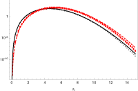
Figure 1: Left panel: Comparison between the analytic functions $\phi^{2}_{\pm}(z_{1})$ and the numerical integral Eq. (III) evaluated by means of the correlated two body intrinsic function. Full line integral over $z_{2}$ of ${}_{2}\phi_{+}(z_{1},z_{2})$. Star points $\phi_{+}(z_{1})$. Dashed line integral over $z_{2}$ of ${}_{2}\phi_{-}(z_{1},z_{2})$. Squared points $\phi_{-}(z_{1})$. Central panel: Full line the ratio ${}_{2}\phi_{+}(z_{1},z_{2}=5~{}\mbox{GeV}^{-1})/_{2}\phi_{-}(z_{1},z_{2}=5~{}\mbox{GeV}^{-1})$, dot-dashed line the ratio ${}_{1}\phi_{+}(z_{1},z_{2}=5~{}\mbox{GeV}^{-1})/_{1}\phi_{-}(z_{1},z_{2}=5~{}\mbox{GeV}^{-1})$. Right panel: the difference between the calculations of the two body intrinsic functions within the correlated and uncorrelated ansatz. Full line: ${}_{1}\phi_{+}(z_{1},z_{2}=5~{}\mbox{GeV}^{-1})-_{2}\phi_{+}(z_{1},z_{2}=5~{}\mbox{GeV}^{-1})$; dot-dashed line: ${}_{1}\phi_{-}(z_{1},z_{2}=5~{}\mbox{GeV}^{-1})-_{2}\phi_{-}(z_{1},z_{2}=5~{}\mbox{GeV}^{-1})$.

For the minus component, one finds

$${}_{2}\phi_{-}(z_{1},z_{2})=\dfrac{D_{4}}{R^{4}}e^{-\kappa^{2}\beta(z_{1},z_{2})/2}\kappa^{7}z_{1}^{5}z_{2}^{5}$$ (17)

$$\times\left.\Big{[}D_{2}U^{2}(-1,1,D_{1}~{}\beta(z_{1},z_{2}))+D_{3}U^{2}(-2,1,D_{1}~{}\beta(z_{1},z_{2}))\right.$$

$$+\left.~{}D_{5}U(-1,1,D_{1}~{}\beta(z_{1},z_{2}))U(-3,1,D_{1}~{}\beta(z_{1},z_{2}))\right.\Big{]}^{1/2}$$

where now the coefficients read:

$$D_{1}=1.48814~{};~{}~{}D_{2}=38.6679~{};~{}~{}D_{3}=0.208628~{};$$

$$D_{4}=0.04298~{};~{}~{}D_{5}=3.73552~{}.$$ (18)

In order to qualitatively show the accuracy of the procedure, in Fig. 1, the integrals over $z_{2}$ of ${}_{2}\phi^{2}_{+}(z_{1},z_{2})$ ( full line) and ${}_{2}\phi^{2}_{-}(z_{1},z_{2})$ (dashed line) are compared to $\phi^{2}_{+}(z_{1})$ ( star points) and $\phi^{2}_{-}(z_{1})$ (squared points) respectively. As one can see the accuracy is quite good for $z_{1}<10$ GeV^-1. With the comfort of these successful checks, in the next section, the result of the calculation of the GPDs at $\xi\neq 0$, within the correlated and uncorrelated ansatz, will be discussed.

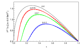
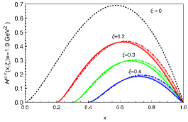
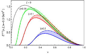
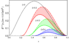
Figure 2: Left panel: the GPDs $H^{u}_{v}(x,\xi,t)$ evaluated at $t=-0.3$ GeV² for four values of $\xi=0,0.05,0.1,0.2$. The full line is obtained by means of the correlated two body intrinsic function, the dot-dashed lines is obtained by means of the uncorrelated one and dotted is obtained for $\xi=0$ (same result obtained and discussed in Ref. gpdsadsqcd ). The band between the two lines represent the theoretical error. Right panel: same quantity of left panel evaluated at $t=-1$ GeV² and $\xi=0,0.2,0.3,0.4$.

Figure 3: Same of Fig. 3 but for the GPDs $E^{u}_{v}(x,\xi,t)$.

V Numerical analysis of the GPDs at $\xi\neq 0$

In this section, the main results of the calculations of the valence GPDs at $\xi\neq 0$ are presented. The difference between the calculations of the GPDs, performed by means of the uncorrelated and correlated scenarios can be considered as the theoretical error of the present approach. In Fig. 3, the GPD $H^{u}_{v}(x,\xi,t)$ has been shown for $t=-0.3$ GeV² (left panel) and $t=-1.0$ GeV² (right panel) for four values of $\xi$ (see caption of Fig. 3). As one can notice, the shape of GPDs, in the $\xi$ dependence, is basically decreasing, qualitatively in agreement with results discussed in Refs. pasquini ; vento , where GPDs have been calculated within constituent quark models. This trend is also confirmed for the GPD $E^{u}_{v}(x,\xi,t)$, see Fig. 3. Same results are found for the flavor $d$. Moreover, for $\xi=0$, as expected, results discussed in Ref. gpdsadsqcd are fully recovered using both the correlated and uncorrelated form of $\phi_{\pm}(z_{1},z_{2})$. Furthermore, for the GPDs $H$, one can notice that the difference between the calculations with the correlated and the uncorrelated two body intrinsic proton functions is quite small. This feature can be understood by looking at the central panel of Fig. 1 where the ratio ${}_{1(2)}\phi_{+}(z_{1},z_{2})/_{1(2)}\phi_{-}(z_{1},z_{2})$ has been shown for $z_{2}=5$ GeV^-1 (approximately the maximum of the distributions). The full line corresponds to the calculation with the correlated ansatz and the dot-dashed one is obtained by means of the uncorrelated two body intrinsic function. As one can see, for small values of $z_{1}$ in both cases the plus component is dominant w.r.t. the minus one. Let us remark that since the bulk-to-boundary propagator, Eq. (II), is peaked around $z_{1}\sim 0$, the integrals Eqs. (III, 12) are dominated by the small $z_{1}$ region. Furthermore, in this range of $z_{1}$, the difference between the correlated and uncorrelated calculations of the plus component of the two body intrinsic function (see the full line in the right panel of Fig. 1) is dramatically small, a feature that explains the small error band in the evaluation of the GPD $H$ in Fig. 3. Regarding the GPD $E$, since in this case, as one can see in Eq. (III), this quantity depends only on the minus component of the two body intrinsic proton function, the error between the correlated and uncorrelated ansatz is bigger then in the plus component case. One can realize such feature by looking at the dot-dashed line in the right panel of Fig. 1. This aspect explains why, in the same kinematic conditions, the error in the calculation of the GPD $E$ is bigger then that in the GPD $H$ case. Let us stress that for both GPDs for very small values of $\xi$ and $t$, the kinematic condition useful to study Ji’s sum rule and the three dimensional partonic structure of the proton, the error in the present approach is quite small. In particular, in this framework, the decreasing trend of the GPDs in the $\xi$ dependence is due to partonic correlations. Furthermore, our analysis shows that if high values of $\xi$ and $t$ are reached in experiments, the GPDs at $\xi\neq 0$ are more sensitive to details of the full proton wave function than form factors or GPDs at $\xi=0$, allowing to access parton correlations usually integrated out in the diagonal case. This analysis has taught us how distributions sensitive to correlations, like GPDs in non forward regions, evaluated thanks to the experience gained in the LF and AdS/QCD approaches, can be used to find the importance of correlations in the structure of hadrons. In further studies, this analysis will be completed by calculating, within the present scheme, other distributions, like dPDFs already investigated within the LF approach jhp1 ; jhp2 ; plb , and which have shown to be sensitive to the kind of correlations here addressed. Work is in progress in that direction. A first evaluation of an approximated expression of dPDFs, through the AdS/QCD correspondence, together with the calculation of an experimental observable is discussed in Ref. effA .

VI Conclusion

In the present analysis, GPDs have been calculated in a fully non forward region, namely $\xi$ and $t$ different from zero. To this aim, the usual strategy, developed to evaluate GPDs at $\xi=0$, within the AdS/QCD correspondence together with the soft-wall model, has been extended in order to evaluate the full proton Light-Front wave function from AdS/QCD, including, in principle, two body correlations. As shown, within this approach, results previously discussed in other analyses have been successfully recovered and the $\xi$ dependence found for the leading twist GPDs $H$ and $E$, evaluated for different flavors, is compatible with the one discussed in calculations with constituent quark models. Furthermore, since in the present study the full proton wave function is obtained by solving an integral equation, different solutions have been scrutinized for the numerical evaluations of GPDs and a discussion on the theoretical error of the approach has been provided. In particular, for small values $\xi$, using different proton wave functions, leading to same form factors and GPDs at $\xi=0$, similar results have been found. However, since at high values of $\xi$, in particular for the GPD $E$, these quantities start to be sensitive to details of the proton structure, e.g., to two body correlations, differences in the calculations of the latter with correlated and uncorrelated distributions become sizable. Results presently discussed demonstrate that in principle new information on partonic structure of hadrons can be obtained from GPDs at $\xi\neq 0$, indirectly accessing two parton correlations, usually studied, e.g. with double parton distribution function in double parton scattering. In closing, our analysis shows that AdS/QCD can be used in the future to estimate other fundamental observables and parton distributions.

References

- (1) D. Müller, D. Robaschik, B. Geyer, F.-M. Dittes and J. Hořejši, Fortsch. Phys. 42, 101 (1994).
- (2) A. V. Radyushkin, Phys. Rev. D 56, 5524 (1997).
- (3) X. D. Ji, Phys. Rev. Lett. 78, 610 (1997).
- (4) M. Diehl, Phys. Rept. 388, 41 (2003).
- (5) M. Burkardt, Int. J. Mod. Phys. A 18, 173 (2003).
- (6) A. Airapetian et al. [HERMES Collaboration], Phys. Rev. Lett. 87, 182001 (2001).
- (7) S. Stepanyan et al. [CLAS Collaboration], Phys. Rev. Lett. 87, 182002 (2001).
- (8) S. J. Brodsky and G. F. de Teramond, Subnucl. Ser. 45, 139 (2009).
- (9) S. J. Brodsky and G. F. de Téramond, Phys. Lett. B 582, 211 (2004).
- (10) G. F. de Teramond and S. J. Brodsky, AIP Conf. Proc. 1257, 59 (2010).
- (11) Z. Abidin and C. E. Carlson, Phys. Rev. D 79, 115003 (2009).
- (12) G. F. de Teramond and S. J. Brodsky, Phys. Rev. Lett. 94, 201601 (2005).
- (13) S. J. Brodsky and G. F. de Teramond, Phys. Rev. D 77, 056007 (2008).
- (14) S. J. Brodsky and G. F. de Teramond, Phys. Rev. D 78, 025032 (2008).
- (15) J. M. Maldacena, Int. J. Theor. Phys. 38, 1113 (1999); Adv. Theor. Math. Phys. 2, 231 (1998); S. S. Gubser, I. R. Klebanov and A. M. Polyakov, Phys. Lett. B 428, 105 (1998); E. Witten, Adv. Theor. Math. Phys. 2, 253 (1998).
- (16) G. F. de Teramond and S. J. Brodsky, Phys. Rev. Lett. 102, 081601 (2009).
- (17) J. Polchinski and M. J. Strassler, Phys. Rev. Lett. 88, 031601 (2002).
- (18) A. Karch, E. Katz, D. T. Son and M. A. Stephanov, Phys. Rev. D 74, 015005 (2006).
- (19) T. Branz, T. Gutsche, V. E. Lyubovitskij, I. Schmidt and A. Vega, Phys. Rev. D 82, 074022 (2010).
- (20) A. Karch, E. Katz, D. T. Son and M. A. Stephanov, Phys. Rev. D 74, 015005 (2006).
- (21) A. Vega and I. Schmidt, Phys. Rev. D 78, 017703 (2008).
- (22) A. Vega and I. Schmidt, AIP Conf. Proc. 1265, 226 (2010).
- (23) A. Vega and I. Schmidt, Phys. Rev. D 79, 055003 (2009).
- (24) D. Chakrabarti and C. Mondal, Eur. Phys. J. C 73, 2671 (2013).
- (25) A. Ballon-Bayona, G. Krein and C. Miller, arXiv:1702.08417 [hep-ph].
- (26) G. F. de Teramond and S. J. Brodsky, arXiv:1203.4025 [hep-ph].
- (27) D. Chakrabarti and C. Mondal, Phys. Rev. D 88, no. 7, 073006 (2013).
- (28) S. J. Brodsky and G. F. de Teramond, Phys. Rev. Lett. 96, 201601 (2006).
- (29) H. Forkel, M. Beyer and T. Frederico, Int. J. Mod. Phys. E 16, 2794 (2007).
- (30) W. de Paula, T. Frederico, H. Forkel and M. Beyer, Phys. Rev. D 79, 075019 (2009).
- (31) A. Vega, I. Schmidt, T. Branz, T. Gutsche and V. E. Lyubovitskij, Phys. Rev. D 80, 055014 (2009).
- (32) S. J. Brodsky, F. G. Cao and G. F. de Teramond, Phys. Rev. D 84, 033001 (2011).
- (33) M. Ahmady and R. Sandapen, Phys. Rev. D 88, 014042 (2013).
- (34) A. Vega, I. Schmidt, T. Gutsche and V. E. Lyubovitskij, Phys. Rev. D 83, 036001 (2011).
- (35) S. J. Brodsky, G. F. de Téramond and H. G. Dosch, Nuovo Cim. C 036, 265 (2013).
- (36) C. Mondal, Eur. Phys. J. C 76, no. 2, 74 (2016).
- (37) J. R. Forshaw and R. Sandapen, Phys. Rev. Lett. 109, 081601 (2012).
- (38) J. Polchinski and M. J. Strassler, JHEP 0305, 012 (2003).
- (39) M. C. Traini, arXiv:1608.08410 [hep-ph].
- (40) M. Ahmady and R. Sandapen, Phys. Rev. D 87, no. 5, 054013 (2013).
- (41) S. Boffi, B. Pasquini and M. Traini, Nucl. Phys. B 649, 243 (2003).
- (42) Z. Fang, D. Li and Y. L. Wu, Phys. Lett. B 754, 343 (2016).
- (43) S. J. Brodsky, H. C. Pauli and S. S. Pinsky, Phys. Rept. 301, 299 (1998).
- (44) S. Scopetta and V. Vento, Eur. Phys. J. A 16, 527 (2003).
- (45) M. Rinaldi, S. Scopetta, M. Traini and V. Vento, JHEP 12, 028 (2014).
- (46) M. Rinaldi, S. Scopetta, M. C. Traini and V. Vento, JHEP 1610, 063 (2016).
- (47) M. Rinaldi, S. Scopetta, M. Traini and V. Vento, Phys. Lett. B 752, 40 (2016).
- (48) M. Traini, M. Rinaldi, S. Scopetta and V. Vento, arXiv:1609.07242, PLB in press.