Direct numerical simulation of variable surface tension flows using a Volume-of-Fluid method

Abstract

We develop a general methodology for the inclusion of variable surface tension into a Volume-of-Fluid based Navier-Stokes solver. This new numerical model provides a robust and accurate method for computing the surface gradients directly by finding the tangent directions on the interface using height functions. The implementation is applicable to both temperature and concentration dependent surface tension, along with the setups involving a large jump in the temperature between the fluid and its surrounding, as well as the situations where the concentration should be strictly confined to the fluid domain, such as the mixing of fluids with different surface tension coefficients. We demonstrate the applicability of our method to thermocapillary migration of bubbles and coalescence of drops characterized by different surface tension.

1 Introduction

Flows induced by the spatial variations in the surface tension, also known as Marangoni effect [1], can be caused by surfactants, temperature or concentration gradients, or a combination of these effects. Understanding these flows is important since they are relevant in microfluidics [2], heat pipe flows [3], motion of drops or bubbles in materials processing applications that include heating or cooling [4], evolution of metal films of nanoscale thickness melted by laser pulses [5, 6], and in a variety of other thin film flows, see [7, 8] for reviews.

Numerical methods for studying variable surface tension flows include front tracking [9], level set [10], diffuse interface [11], marker particle [12, 13], immersed boundary [14], boundary integral [15], interface-interaction [16], and Volume-of-Fluid (VOF) [17, 18, 19] methods. The VOF method is efficient and robust for tracking topologically complex evolving interfaces. The improvements in recent years in the computation of the surface tension have empowered the VOF method to become a widespread method for modeling interfacial flows [20, 21]. However, an accurate implementation of the variable surface tension in the VOF formulation is still lacking a general treatment.

A challenge of including variable surface tension effects into the VOF method is that the surface tension is not known exactly at the interface - only the value averaged over a computational cell containing the interface is known. To obtain the surface tension at the interface, an approximation from the values near the interface, usually calculated at the center of each adjacent computational cell, is necessary. As we outline below, the approximation of the interface values has been carried out in the literature differently, depending on the physics of the problem studied. Additional major issue concerns computing the surface gradients of the surface tension.

In Alexeev et al. [22] and Ma and Bothe [19], the VOF method is used to study flows involving temperature dependent surface tension. The implementation in Alexeev et al. [22] solves the heat equation in fluids on the both sides of the interface, and then imposes the continuity of the temperature and flux at the interface, and conservation of energy in the cell containing the interface to approximate the temperature in the fluid and air in the cell. These temperature values are then used to calculate surface gradients of the temperature from nearby cells that are not cut by the interface; these gradients are then exponentially extrapolated to the interface. In the work by Ma and Bothe [19], the temperature at the interface is approximated from the temperatures in the liquid and the gas by imposing the continuity of heat flux at the interface. The surface gradients of the temperature are approximated by computing the derivatives in each coordinate direction using finite differences, and then projecting them onto the tangential direction. If the interface is not contained in all cells of the finite difference stencil, then one sided differences are used. Hence, this method requires temperature solution on both sides of the interface and therefore cannot be used for the setups involving a large difference in thermal conductivity of the two fluids, since the fluids may have a large difference in the temperature. Furthermore, both of these methods are not applicable to setups where the surface tension only depends on the concentration, such as mixing of miscible liquids with different surface tension. In the work by James and Lowengrub [18], the VOF method is used to study the flows induced by the surfactant concentration gradient. In their method, the concentration values at the interface are obtained by imposing the condition that the average concentration at the interface is equal to the average concentration in the cell containing the interface. Then, the surface gradients are computed using the cell-center interfacial concentration in the two adjacent cells.

Here, we develop a method that can be applied to both temperature and concentration dependent surface tension, with the surface gradients computed using the cell-center values in the interfacial cells only. We find the tangential gradients directly by computing the tangent directions on the interface using height functions [23]. This method can be applied to the setups such that the concentration is confined to the fluid domain, e.g. mixing of liquids with different surface tension coefficients, as well as the configurations involving large jump of the temperature between the liquid and the surrounding. Since our method does not depend on whether we consider temperature or concentration gradients, we will use them interchangeably in the remaining part of the paper.

Our numerical method is implemented using Gerris: an open source adaptive Navier-Stokes solver [24, 23]. The current version includes Continuum Surface Force (CSF) [25] implementation of the surface tension force with height function algorithm for computing interfacial normal and curvature [23]. Here, we present the method for extending this formulation to include variable surface tension, allowing to consider the surface force in the direction tangential to the interface. As far as we are aware, this is the first implementation of the variable surface tension combined with the accurate implementation of the CSF method, such that the curvature and interface normals are computed using generalized height functions [23]. Our extension is a step closer to cover all aspects of the variable surface tension flows; the remaining one is the implementation of the surfactant transport and surface tension gradients due to the presence of the surfactants. This will be the topic of our future work.

The rest of this paper is organized as follows: Section 2 gives an overview of the VOF method, including the CSF method for the computation of the surface tension; Section 3 describes in detail the implementation of the variable surface tension in two and three dimensions; and Section 4 illustrates the performance of our method for various test cases, including temperature and concentration dependent surface tension.

2 Governing equations

We consider incompressible two-phase flow described by Navier-Stokes equations

$$\rho(\partial_{t}\textbf{u}+\textbf{u}\cdot\nabla\textbf{u})=-\nabla p+\nabla\cdot\left(2\mu D\right)+\textbf{F},$$ (1)

$$\nabla\cdot\textbf{u}=0,$$ (2)

and the advection of the phase-dependent density $\rho\left(\chi\right)$

$$\partial_{t}\rho+(\textbf{u}\cdot\nabla)\rho=0,\,$$ (3)

where $\textbf{u}=(u,v,w)$ is the fluid velocity, $p$ is the pressure, $\rho(\chi)=\chi\rho_{1}+(1-\chi)\rho_{2}$ and $\mu(\chi)=\chi\mu_{1}+(1-\chi)\mu_{2}$ are the phase dependent density and viscosity respectively, and $D$ is the rate of deformation tensor $D=\left(\nabla\textbf{u}+\nabla\textbf{u}^{T}\right)/2$. Subscripts $1$ and $2$ correspond to the fluids $1$ and $2$, respectively (see Figure 1). Here, $\chi$ is the characteristic function, such that $\chi=1$ in the fluid $1$, and $\chi=0$ in the fluid $2$. Note that any body force can be included in F. The characteristic function is advected with the flow, thus

$$\partial_{t}\chi+(\textbf{u}\cdot\nabla)\chi=0.$$ (4)

Note that solving equation (4) is equivalent to solving equation (3).

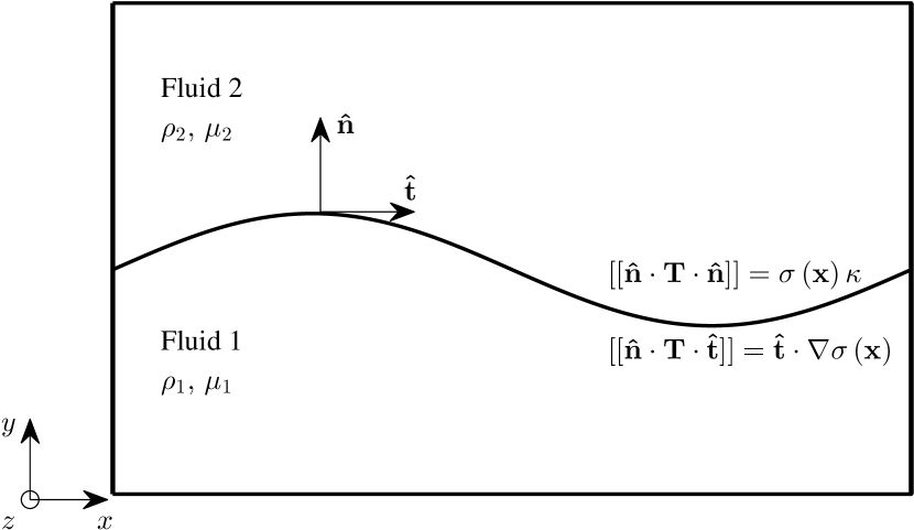
Figure 1: Schematic of a system with two immiscible fluids and the corresponding boundary conditions.

The presence of an interface gives rise to the stress boundary conditions, see Figure 1. The normal stress boundary condition at the interface defines the stress jump [26, 27]

$$\llbracket\hat{\mathbf{n}}\cdot\mathbf{T}\cdot\hat{\mathbf{n}}\rrbracket=\sigma\left(\mathbf{x}\right)\kappa,$$ (5)

where $\mathbf{T}=-p\mathbf{I}+\mu\left(\nabla\textbf{u}+\nabla\textbf{u}^{T}\right)$ is the total stress tensor, $\sigma\left(\mathbf{x}\right)$ is the surface tension coefficient, $\kappa$ is the curvature of the interface, and $\hat{\mathbf{n}}$ is the unit normal at the interface pointing out of the fluid 1. The variation of surface tension coefficient results in the tangential stress jump at the interface

$$\llbracket\hat{\mathbf{n}}\cdot\mathbf{T}\cdot\hat{\mathbf{t}}\rrbracket=\hat{\mathbf{t}}\cdot\mathbf{\nabla}\sigma\left(\mathbf{x}\right),$$ (6)

which drives the flow from the regions of low surface tension to the ones with high surface tension. Here, $\hat{\mathbf{t}}$ is the unit tangent vector in two dimensions (2D); in three dimensions (3D) there are two linearly independent unit tangent vectors. Using the Continuum Surface Force (CSF) method [25], the forces resulting from the normal and tangential stress jump at the interface can be included in the body force $\textbf{F}=\textbf{F}_{sn}+\textbf{F}_{st}$, defined as

$$\textbf{F}_{sn}=\sigma\left(\mathbf{x}\right)\kappa\delta_{s}\hat{\mathbf{n}},$$ (7)

and

$$\textbf{F}_{st}=\mathbf{\nabla}_{s}\sigma\left(\mathbf{x}\right)\delta_{s},$$ (8)

where $\delta_{s}$ is the Dirac delta function centered at the interface, $\delta_{s}\hat{\mathbf{n}}=\nabla\chi$, and $\mathbf{\nabla}_{s}$ is the surface gradient. Substituting equations (7) and (8) in the momentum equation (1) gives

$$\rho(\partial_{t}\textbf{u}+\textbf{u}\cdot\nabla\textbf{u})=-\nabla p+\nabla\cdot\left(2\mu D\right)+\sigma\left(\mathbf{x}\right)\kappa\delta_{s}\hat{\mathbf{n}}+\mathbf{\nabla}_{s}\sigma\left(\mathbf{x}\right)\delta_{s}.$$ (9)

We define the nondimensional variables, denoted with a superscript “*”, as

$$\begin{aligned} x^{*}=\frac{x}{a},\,\,\,\,t^{*}=\frac{t}{t_{r}},\,\,\,\,\mathbf{u}^{*}=\frac{\mathbf{u}}{U_{0}},\,\,\,\,p^{*}=\frac{p}{p_{0}},\\ \rho^{*}\left(\chi\right)=\frac{\rho\left(\chi\right)}{\rho_{1}},\,\,\,\,\mu^{*}\left(\chi\right)=\frac{\mu\left(\chi\right)}{\mu_{1}},\,\,\,\,\sigma^{*}=\frac{\sigma}{\sigma_{0}},\end{aligned}$$

where the scales $a$, $p_{0}$, $t_{c}$, $U_{0}$ and $\sigma_{0}$ are chosen based on the problem studied. Hence the dimensionless equation (9) is

$$\text{Re}\rho^{*}(\partial_{t}^{*}\mathbf{u}^{*}+\mathbf{u}^{*}\cdot\nabla^{*}\mathbf{u}^{*})=-\nabla^{*}p^{*}+\nabla^{*}\cdot\left(2\mu^{*}D^{*}\right)+\\ +\text{Ca}^{-1}\sigma^{*}\kappa^{*}\delta_{s}^{*}\hat{\mathbf{n}}+\frac{\sigma_{0}}{U_{0}\mu_{1}}\nabla_{s}^{*}\sigma^{*}\delta_{s}^{*}\hat{\mathbf{t}},$$ (10)

where Re and Ca are the Reynolds and Capillary numbers respectively, defined as

$$\text{Re}=\frac{\rho_{1}U_{0}a}{\mu_{1}},\,\,\,\,\,\text{Ca}=\frac{U_{0}\mu_{1}}{\sigma_{0}}.$$ (11)

The surface tension is a function of temperature, $T$, or concentration, $C$, which satisfy advection diffusion equation

$$\rho\left(\chi\right)C_{p}\left(\chi\right)\left(\partial_{t}T+(\textbf{u}\cdot\nabla)T\right) =\nabla\cdot\left(k\left(\chi\right)\nabla T\right),$$ (12)

$$\partial_{t}C+(\textbf{u}\cdot\nabla)C =\nabla\cdot\left(\alpha\left(\chi\right)\nabla C\right),$$ (13)

where $C_{p}\left(\chi\right)$, $k\left(\chi\right)$ and $\alpha\left(\chi\right)$ are the phase dependent heat capacity, conductivity and diffusivity, respectively. Along with the scales given above, equations (12) and (13) are nondimensionalized using the following scales

$$k^{*}\left(\chi\right)=\frac{k\left(\chi\right)}{k_{1}},\,\,\,\,C_{p}^{*}\left(\chi\right)=\frac{C_{p}\left(\chi\right)}{C_{p_{1}}},\,\,\,\,T^{*}=\frac{T}{T_{0}},\,\,\,\,\alpha^{*}\left(\chi\right)=\frac{\alpha\left(\chi\right)}{\alpha_{1}},$$ (14)

where $T_{0}$ is chosen based on the physics of the system. Hence the dimensionless equations (12) and (13) are

$$\text{Ma}\rho^{*}C_{p}^{*}\left(\partial_{t}^{*}T^{*}+(\mathbf{u}^{*}\cdot\nabla^{*})T^{*}\right)=\nabla^{*}\cdot\left(k^{*}\nabla^{*}T^{*}\right),$$ (15)

$$\text{Ma}\left(\partial_{t}^{*}C^{*}+(\mathbf{u}^{*}\cdot\nabla^{*})C^{*}\right)=\nabla^{*}\cdot\left(\alpha^{*}\nabla^{*}C^{*}\right),$$ (16)

where Ma is the Marangoni number defined as

$$\text{Ma}=\frac{U_{0}a}{\alpha_{1}}.$$ (17)

The diffusivity, $\alpha_{1}$, in the heat equation is $\alpha_{1}={k_{1}}/({\rho_{1}C_{p_{1}}})$. Surface tension can have linear or nonlinear dependence on temperature or concentration. In many applications the surface tension depends on the temperature linearly, i.e.

$$\sigma=\sigma_{0}+\sigma_{T}\left(T-T_{R}\right),$$ (18)

where $\sigma_{0}$ is the surface tension at a reference temperature $T_{R}$, and $\sigma_{T}$ is a constant. Then, we can write

$$\mathbf{\nabla}_{s}\sigma=\sigma_{T}\mathbf{\nabla}_{s}T,$$ (19)

and compute $\mathbf{\nabla}_{s}T$ in the same manner as $\mathbf{\nabla}_{s}\sigma$. Using the scales given above, the dimensionless equation (18) is

$$\sigma^{*}=1+\frac{\sigma_{T}T_{0}}{\sigma_{0}}\left(T^{*}-T_{R}^{*}\right).$$ (20)

In the following section, we describe a method for computing $\nabla_{s}\sigma$ in general, regardless of the dependence on the temperature or concentration.

3 Numerical method

The proposed numerical method is implemented into Gerris, which numerically solves equations (1) to (3) using the VOF interface tracking method with implicit treatment of the viscous forces [23, 24, 28]. The CSF method is used for the implementation of the surface tension force with curvatures computed using the height function method [23, 29]. The Gerris code uses octree (3D) and quadtree (2D) grids, allowing to adaptively refine the grid in the immediate neighborhood of the interface. While we describe our implementation of the variable surface tension for uniform meshes, the extension to adaptively refined meshes is straightforward, following the implementation details described by Popinet [23, 24].

The surface gradient of any scalar field $Q$ is defined as the projection of the gradient onto the surface, i.e.

$$\nabla_{s}Q=\nabla Q-\hat{\mathbf{n}}\left(\hat{\mathbf{n}}\cdot\nabla Q\right)$$ (21)

where $\hat{\mathbf{n}}$ is the unit normal vector at the surface. However, this definition of the surface gradient can result in inaccuracies when implemented in the VOF method for general variable surface tension for two reasons. First, the discontinuities of the material properties across the interface can result in $Q$ having a large jump across the interface: for example, in the case of surface tension dependence on the temperature where the fluids on each side of the interface have large difference in the conductivity. The second reason is that, in general, surface tension can depend on the concentration: for example, in the case of the mixing of two liquids with different surface tension, or in the case of surface tension dependent on the surfactant concentration.

Here, we propose a numerical method for implementing the general variable surface tension. We compute the surface gradient as

$$\textbf{F}_{st}=\frac{\partial\sigma}{\partial s_{1}}\delta_{s}\hat{\mathbf{t}}_{1}+\frac{\partial\sigma}{\partial s_{2}}\delta_{s}\hat{\mathbf{t}}_{2},$$ (22)

where $\hat{\mathbf{t}}_{1}$ and $\hat{\mathbf{t}}_{2}$ are the unit tangent vectors at the interface, pointing in the $s_{1}$ and $s_{2}$ directions, respectively. In our approach, we first define surface tension values at the interface, then compute the derivatives of $\sigma$ along the interface, and finally project the derivatives onto the tangent space defined by $\hat{\mathbf{t}}_{1}$ and $\hat{\mathbf{t}}_{2}$. In the following Sections we present the details of the implementation. In Section 3.1, we show how to approximate the surface tension value on the interface using the cell-center values. Then in Section 3.2, we show how ${\partial\sigma}/{\partial s_{d}}$, for $d=1,2$, are evaluated, along with the choice of the tangent vectors and addition of the tangential surface force using CSF method. This is done first for 2D is Section 3.2.1, and then for 3D in Section 3.2.2.

3.1 Approximation of interfacial values of surface tension

The algorithm for implementing $\nabla_{s}\sigma\left(\mathbf{x}\right)$ in the VOF method starts with the approximation of the interfacial values of the surface tension in each cell containing an interface segment. More precisely, we use the idea of constructing the columns of cells inspired by the computation of interfacial curvature and normals using height functions [23] (see A.1).

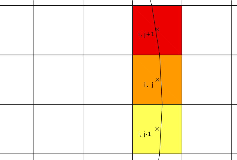
(a)

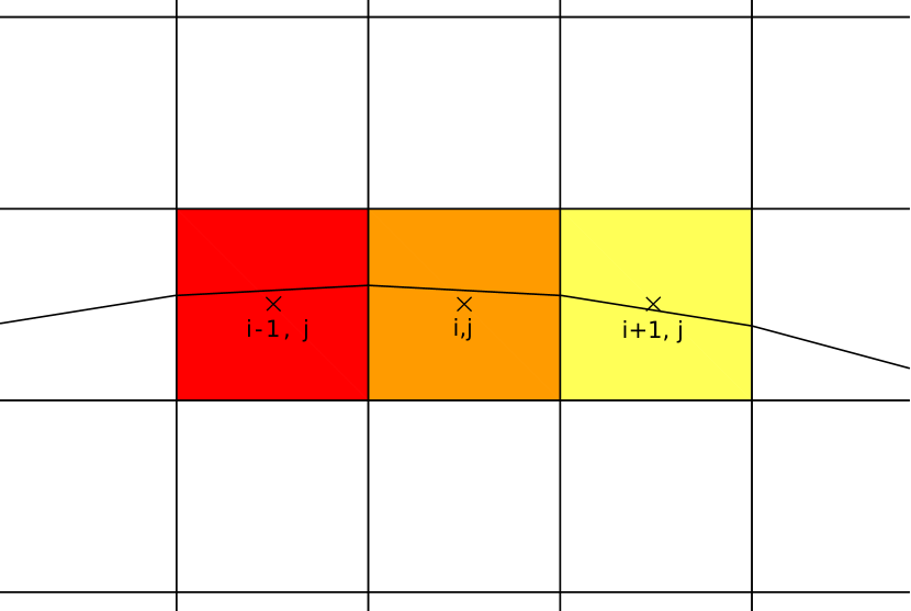
(b)

Figure 2: An example of the interface orientation, where columns in $x$ (a) and $y$ (b) direction for computing $\tilde{\sigma}^{c}\left(\mathbf{x}\right)$ contain one interfacial cell. Each color shows a different column in interfacial cells $\mathcal{C}$.

Let $\sigma({\mathcal{C}})$ be the surface tension evaluated from the temperature or concentration at the center of all interfacial cells $\mathcal{C}$, with the volume fraction $\chi(\mathcal{C})$. The surface tension in each column, denoted by $\tilde{\sigma}^{c}\left(\mathbf{x}\right)$, is defined so that it has only one value in each column, regardless of how many interfacial cells are contained in that column. For illustration, Figure 2 shows columns that contain only one interfacial cell, and Figure 3 shows columns that contain more than one interfacial cell, where the same color denotes cells in the same column. The superscript, $c=x,y,z$, represents the column direction. For simplicity, here we show examples of the implementation in 2D, however, the algorithm extends trivially to 3D.

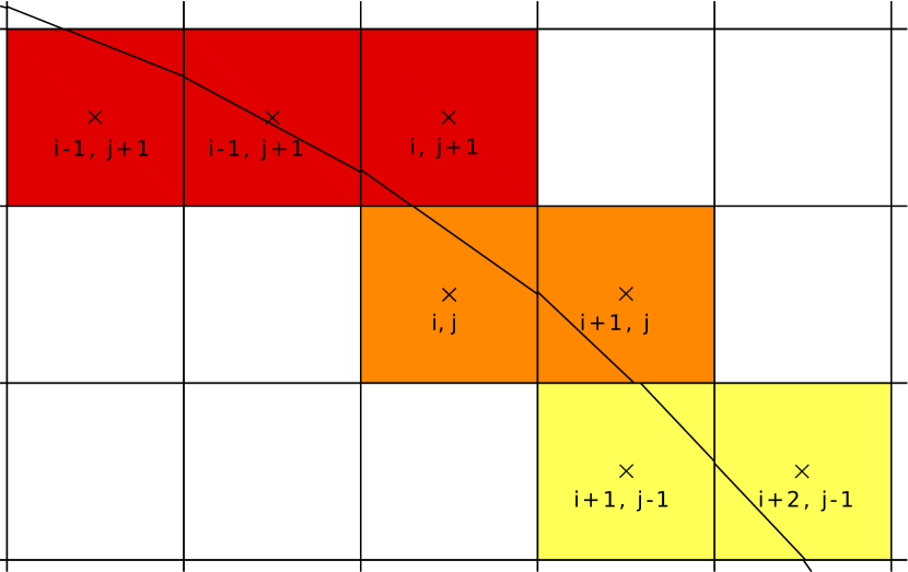
(a)

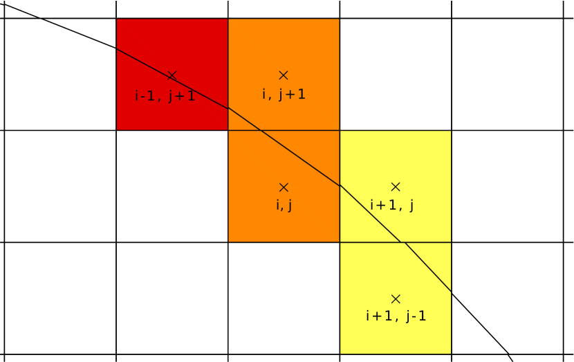
(b)

Figure 3: An example of the interface orientation where columns in $x$ (a) and $y$ (b) direction for computing $\tilde{\sigma}^{c}$ contain more than one interfacial cell. The cells with the same color belong to the same column.

For columns with only one interfacial cell (see Figure 2(a) and (b) for the columns in $x$ and $y$ direction, respectively), the surface tension of the interfacial cells, $\tilde{\sigma}^{c}$, is equal to the surface tension $\sigma({\mathcal{C}})$ in the same cells. If there is more than one interfacial cell in the column, then $\tilde{\sigma}^{c}$ is approximated by the volume weighted average of the $\sigma({\mathcal{C}})$ values. In Figure 3, the cells labeled with cell indices will be used for computing $\tilde{\sigma}^{c}$ for columns in the $x$ and $y$ directions – Figures 3(a) and (b) respectively. For example, in Figure 3(a), the $\tilde{\sigma}^{x}$ is computed using the columns in the $x$ direction, and the value of $\tilde{\sigma}^{x}$ in the column containing cell $\mathcal{C}_{i,j}$, denoted $\tilde{\sigma}_{j}^{x}$, is

$$\tilde{\sigma}_{j}^{x}=\frac{\chi_{i,j}\sigma_{i,j}+\chi_{i+1,j}\sigma_{i+1,j}}{\sum\chi_{i}}.$$ (23)

Note that the cells in the same column, in this particular example cells $\mathcal{C}_{i,j}$ and $\mathcal{C}_{i+1,j}$, have the same value of $\tilde{\sigma}^{x}$. For the columns in the $y$ direction, as in Figure 3(b), $\tilde{\sigma}^{y}$ in the column containing cell $\mathcal{C}_{i,j}$, denoted $\tilde{\sigma}_{i}^{y}$, is computed as

$$\tilde{\sigma}_{i}^{y}=\frac{\chi_{i,j}\sigma_{i,j}+\chi_{i,j+1}\sigma_{i,j+1}}{\sum\chi_{i}}.$$ (24)

Again, the cells in the same column, in this case $\mathcal{C}_{i,j}$ and $\mathcal{C}_{i,j+1}$ have the same value of $\tilde{\sigma}^{y}$.

In our implementation, we first define $\tilde{\sigma}^{c}$ for all $c$ in all interfacial cells. For certain interface orientations, it is possible to define $\tilde{\sigma}^{c}$ for columns in more than one direction, e.g. the interface in Figure 3. However, this is not always the case, e.g. in Figure 2(a) we can only compute $\tilde{\sigma}^{x}$, and in Figure 2(b) we can only compute $\tilde{\sigma}^{y}$. For the former case, in the following sections we describe how the direction of the columns is chosen along with the discussion of the computation of the surface forces.

3.2 Computation of the surface forces

The next step in the variable surface force implementation is the evaluation of the derivatives along the interface, ${\partial\sigma}/{\partial s_{d}}$ in equation (22). In 2D, we only need to compute the derivative in one direction, since the basis for a tangent line consists of only one vector. However, in 3D, we need two tangent vectors to form a basis for the tangent space, hence we need to evaluate the derivative in two directions. We now discuss the implementation of the method for 2D and 3D.

3.2.1 Surface force in 2D

In 2D, equation (22) simplifies to

$$\textbf{F}_{st}=\frac{\partial\sigma}{\partial s^{c}}\delta_{s}\hat{\mathbf{t}},$$ (25)

since we only have one tangential direction. We remind the reader that in this case, $c=x,y$. The derivative of the surface tension along the interface, ${\partial\sigma}/{\partial s^{c}}$, is approximated by the derivative of the interfacial value, $\tilde{\sigma}^{c}$ in the column which is formed in the direction $c$. The choice of the direction, $c$, is based on the interface orientation: $c$ is chosen to be the same as the largest component of the normal vector to the interface. The same choice is made for computing curvature and the interface normal using height functions [23].

In each interfacial cell, we compute the derivative along the interface using center difference, i.e. the finite difference of the $\tilde{\sigma}^{c}$ in the two neighboring columns. For example, in Figure 2(a) and 3(a), the derivative is computed with respect to the $y$ direction, as

$$\left(\frac{\partial\sigma}{\partial s^{x}}\right)_{i,j}=\frac{\tilde{\sigma}_{j+1}^{x}-\tilde{\sigma}_{j-1}^{x}}{\text{d}s}.$$ (26)

As a reminder, $\tilde{\sigma}_{j}^{x}$ is the interfacial value of the surface tension in the column $j$ constructed in the $x$ direction. The arc length, $\text{d}s$, is computed from the height function in the same direction as ${\partial\sigma}/{\partial s^{c}}$. For the example given in equation (26), the arc length is

$$\text{d}s=2\Delta\sqrt{1+h_{y}},$$ (27)

where $h_{y}$ is the derivative of the height function (see A.1) and $\Delta$ is the cell size.

The next part of the surface gradient implementation is the choice of the tangent vector, $\hat{\mathbf{t}}$, which is computed so that it satisfies $\hat{\mathbf{t}}\cdot\hat{\mathbf{n}}=0$, where $\hat{\mathbf{n}}$ is found using Mixed Young’s Center method by Aulisa et al. [30]. The direction of $\hat{\mathbf{t}}$ depends on the direction used for computing ${\partial\sigma}/{\partial s^{c}}$: $\hat{\mathbf{t}}$ points in the direction of the positive component orthogonal to the $c$ direction. For example, $\hat{\mathbf{t}}$ points in the positive $x$ direction if we construct columns in the $y$ direction.

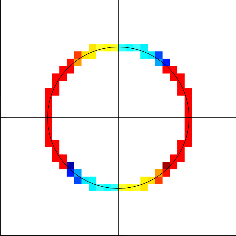
(a)

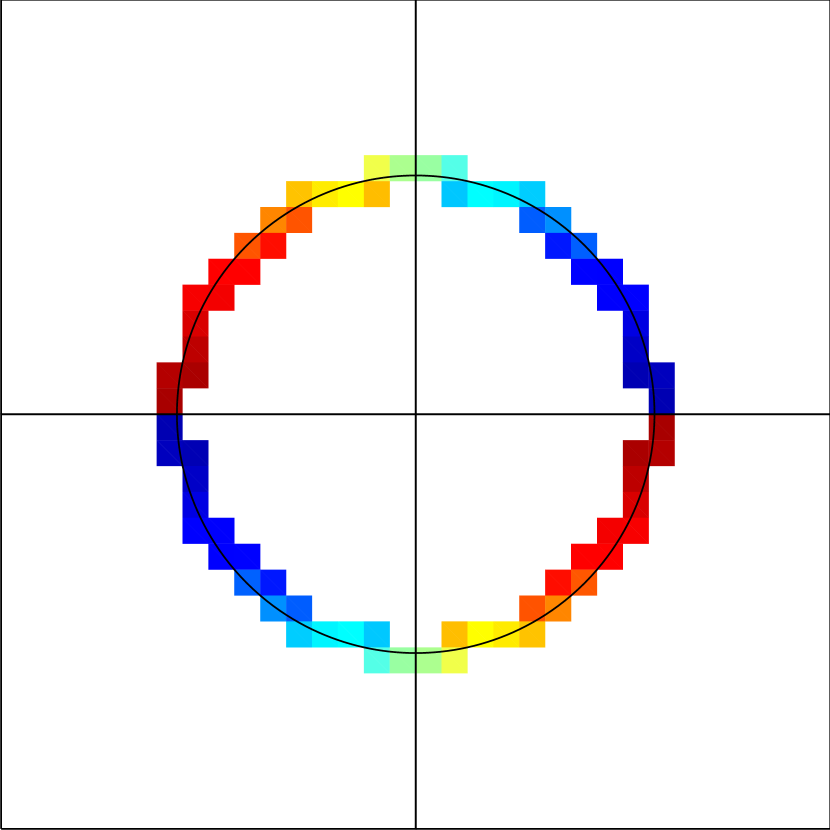
(b)

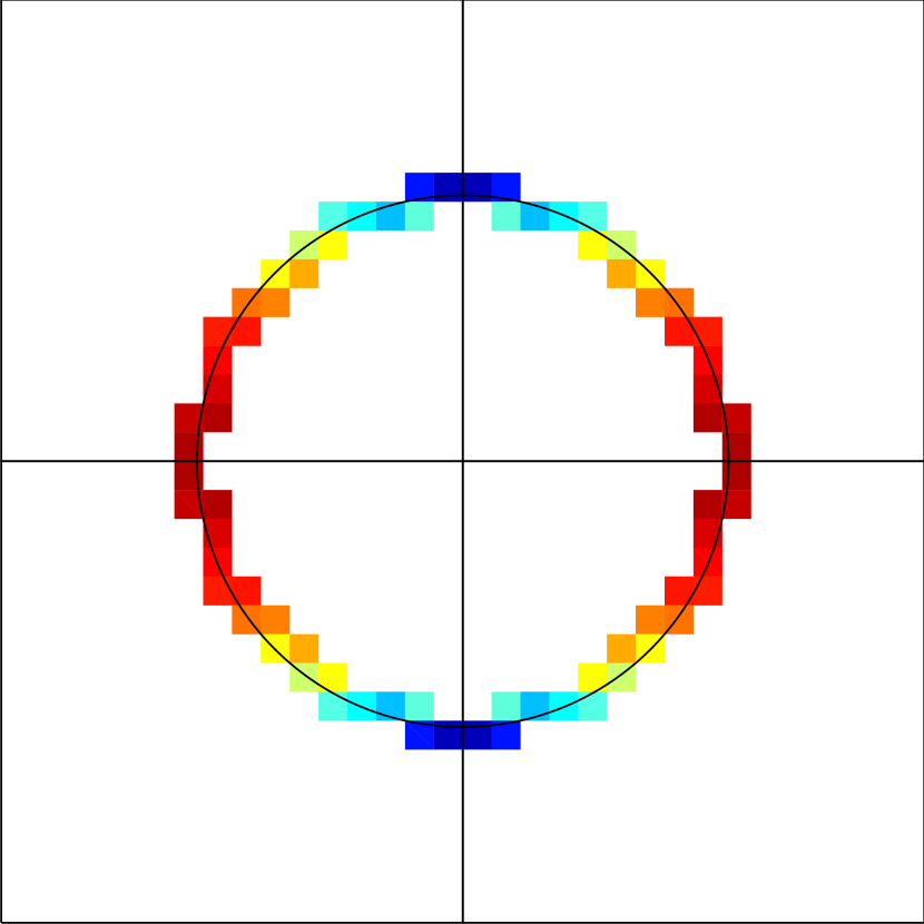
(c)

Figure 4: (a) Example of the gradient ${\partial\sigma}/{\partial s^{c}}$, computed on a circular interface, where $\sigma$ depends on the $y$ direction linearly. The dark red and dark blue colors are the most positive and negative values respectively. The $x$ (b) and $y$ (c) components of $\mathbf{G}$.

To illustrate the importance of the choice of the tangent vector, consider an intermediate value of the surface force, $\mathbf{G}$, defined as

$$G_{x}=\frac{\partial\sigma}{\partial s^{c}}\text{sgn}(t_{x}),$$ (28)

$$G_{y}=\frac{\partial\sigma}{\partial s^{c}}\text{sgn}(t_{y}).$$ (29)

Figure 4(a), (b) and (c) show an examples of ${\partial\sigma}/{\partial s^{c}}$, $G_{x}$ and $G_{y}$ respectively, computed in all interfacial cells, where we impose a positive uniform gradient of the surface tension in the $y$ direction. In figure 4(a), ${\partial\sigma}/{\partial s^{c}}$ changes sign in the first and third quadrant at the angles, defined from the positive $x$ axis, of $\pi/4$ and $5\pi/4$, respectively. At these points the direction of the columns used in gradient computation changes. Hence, the two neighboring cells have opposite sign of ${\partial\sigma}/{\partial s^{c}}$. However, once we include the correct sign of the tangent vector components and consider each component separately, as in equations (28) and (29), this inconsistency in the sign is corrected; see Figure 4(b) and (c) for illustration.

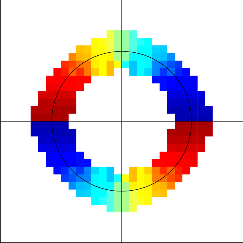
(a)

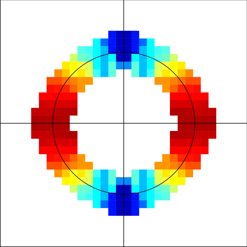
(b)

Figure 5: The $x$ (a) and $y$ (b) component of $\mathbf{G}$, with values around the interfacial cells defined by averaging the neighboring cells.

The complete surface force defined in equation (25), given in the component form, is

$$F_{x}=G_{x}|t_{x}|\,\delta_{s},$$ (30)

$$F_{y}=G_{y}|t_{y}|\,\delta_{s}.$$ (31)

where $\delta_{s}=||\nabla\chi||_{2}$. In the CSF method [25], we need to know $\mathbf{G}$ in the cells around the interface, i.e. in all the cells where $||\nabla\chi||_{2}$ is nonzero. We proceed by using the same approach as for defining the curvature in the cells around the interface [28], i.e. the values in the cells neighboring the interfacial cells are defined by averaging the values in the direct neighbors that already have the curvature value defined. This procedure is repeated twice, insuring that the curvature values for the corner neighbors to the interfacial cells are defined as well. We use an identical approach for defining the $x$ and $y$ components of $\mathbf{G}$ in the cells around the interface which are subsequently used in equations (30) and (31). Figure 5 shows the result of this procedure for the same example of the surface gradient as discussed in Figure 4.

3.2.2 Surface force in 3D

The implementation of the surface gradient in 3D extends the 2D implementation by considering the second tangential direction as stated in equation (22). Equivalently as in 2D, we first define the column values $\tilde{\sigma}^{c}$ of the surface tension $\sigma$. This part of the algorithm is identical to the 2D part, with the addition of one more direction. After the column values, $\tilde{\sigma}^{c}$, are defined, we compute the gradients along the two components orthogonal to the columns: for example, if the columns are constructed in the $z$ direction, see Figure 6, then the derivatives along the interface are computed in the $x$ and $y$ directions as

$$\left(\frac{\partial\sigma}{\partial s^{z}_{1}}\right)_{i,j} =\frac{\tilde{\sigma}_{i+1,j}^{z}-\tilde{\sigma}_{i-1,j}^{z}}{2\Delta\sqrt{1+h_{x}^{2}}},$$ (32)

$$\left(\frac{\partial\sigma}{\partial s^{z}_{2}}\right)_{i,j} =\frac{\tilde{\sigma}_{i,j+1}^{z}-\tilde{\sigma}_{i,j-1}^{z}}{2\Delta\sqrt{1+h_{y}^{2}}}.$$

As previously discussed in 2D, the direction, $c$, in which the columns are constructed, is chosen based on the interface orientation, where $c$ is the same as the direction of the largest component of the interface normal vector.

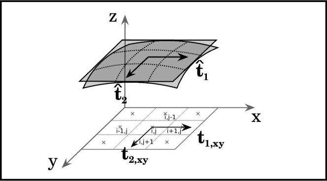
Figure 6: A stencil used for computing surface gradient in the column containing the cell $\mathcal{C}_{i,j}$, with a tangent plane defined by the vectors $\hat{\mathbf{t}}_{1}$ and $\hat{\mathbf{t}}_{2}$. Vectors $\hat{\mathbf{t}}_{1,xy}$ and $\hat{\mathbf{t}}_{2,xy}$ are the projections of $\hat{\mathbf{t}}_{1}$ and $\hat{\mathbf{t}}_{2}$ onto the $xy$-plane respectively.

Next part of the surface gradient computation is the choice of the tangent vectors, $\hat{\mathbf{t}}_{d}$, which are computed so that they satisfy $\hat{\mathbf{t}}_{d}\cdot\hat{\mathbf{n}}=0$. Among all the possibilities for $\hat{\mathbf{t}}_{d}$, we choose the two whose projections onto the coordinate plane, defined by all points with $c$ coordinate equal to zero, are parallel to the axes. Figure 6 illustrates this procedure by an example where the columns are constructed in the $z$ direction and the projections of the tangent vectors $\hat{\mathbf{t}}_{1}$ and $\hat{\mathbf{t}}_{2}$ onto the $x$-$y$ plane are parallel to the $x$ and $y$ axes and denoted by $\hat{\mathbf{t}}_{1,xy}$ and $\hat{\mathbf{t}}_{2,xy}$, respectively. In this particular example, the tangent vectors will be of the form

$$\hat{\mathbf{t}}_{1}=(t_{1x},0,t_{1z}),$$ (33)

$$\hat{\mathbf{t}}_{2}=(0,t_{2y},t_{2z}).$$ (34)

The signs of the components of the tangential vectors are chosen so that their projections onto the coordinate plane point in the positive direction of the coordinate axes (see e.g. Figure 6).

Finally, we compute the surface force, $\textbf{F}_{st}=(F_{x},F_{y},F_{z})$. In the case such that the columns are constructed in the $z$ direction, the components of $\textbf{F}_{st}$ are

$$F_{x} =\frac{\partial\sigma}{\partial s^{z}_{1}}t_{1x},$$ (35)

$$F_{y} =\frac{\partial\sigma}{\partial s^{z}_{2}}t_{2y},$$ (36)

$$F_{z} =\frac{\partial\sigma}{\partial s^{z}_{1}}t_{1z}+\frac{\partial\sigma}{\partial s^{z}_{2}}t_{2z}.$$ (37)

Similarly as in the 2D case, in order to use the CSF formulation, the components of the tangential force need to be defined in the cells around the interface. This is done equivalently as in 2D, using the neighbor averaging procedure, see Section 3.2.1. However, in 3D, there is one extra step due to one of the components containing an addition of two terms, e.g. as in equation (37). In order to illustrate this, consider the general form of the $x$ component of the tangential force

$$F_{x}=\begin{cases}(\partial\sigma/\partial s^{x}_{1})t_{1x}+(\partial\sigma/\partial s^{x}_{2})t_{2x}&\mbox{ if }c=x,\\ (\partial\sigma/\partial s^{y}_{1})t_{1x}&\mbox{ if }c=y,\\ (\partial\sigma/\partial s^{z}_{1})t_{1x}&\mbox{ if }c=z.\end{cases}$$ (38)

Similarly as in 2D, the differences in the sign in the derivatives, $\partial\sigma/\partial s^{c}_{d}$, may arise from the choice of the column directions. We proceed by defining the intermediate value of the surface force, $\mathbf{G}$. The components of $\mathbf{G}$ are computed equivalently as in 2D, except for the $c$ component which is defined as

$$G_{c}=\frac{(\partial\sigma/\partial s^{c}_{1})t_{1c}+(\partial\sigma/\partial s^{c}_{2})t_{2c}}{\sqrt{t_{1c}^{2}+t_{2c}^{2}}},$$ (39)

where $c$ is the direction of the columns. Now we can carry out the averaging procedure for each component of $\mathbf{G}$. Finally, the component of the force in the direction $c$ is

$$F_{c}=G_{c}|t_{1c}|\delta_{s}+G_{c}|t_{2c}|\delta_{s}.$$ (40)

The other components are computed equivalently as in the 2D case.

4 Results

4.1 Surface gradient computation

We first present the validation of our methodology for computing the surface gradient in 2D geometry where we can compute the gradient exactly. The simplest geometry that we consider is a flat perturbed interface, i.e. let the interface be a function of $x$ as

$$h\left(x\right)=h_{0}+\varepsilon\cos(2\pi x).$$ (41)

Let the surface tension be a function of the interface position as

$$\sigma\left(h\right)=1+\sigma_{h}h\left(x\right),$$ (42)

Figure 7 shows the interface profile and surface tension at the interface, for $h_{0}=0.5$, $\varepsilon=0.05$, and $\sigma_{h}=10^{-2}$ in a computational domain of $1\times 1$, with symmetry boundary conditions imposed on all sides.

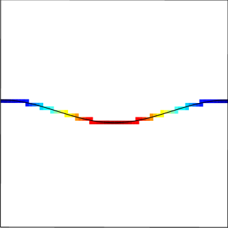
Figure 7: The setup of the perturbed interface with surface tension dependent on the interface profile $h\left(x\right)=h_{0}+\varepsilon\cos(2\pi x)$. The color represents the surface tension at the interface, with dark red and dark blue being the maximum and minimum values respectively.

In this case, apart from using the definition of the surface gradient given in equation (21), we can also compute the exact surface gradient using the chain rule as

$$\nabla_{s}\sigma=\frac{\sigma_{h}h_{x}}{\sqrt{1+h_{x}^{2}}}\,\hat{\mathbf{t}},$$ (43)

where the unit tangent vector, $\hat{\mathbf{t}}$, is defined to point in the positive $x$ direction as

$$\hat{\mathbf{t}}=\left(1,-h_{x}\right)/\sqrt{1+h_{x}^{2}},$$ (44)

Note that the numerator in equation (43), $\sigma_{h}h_{x}$, is equivalent to the numerator of equation (26); hence, we can compare their computed values to the exact ones directly. We present the errors associated with computing $\sigma_{h}h_{x}$ and $h_{x}$, separately, as well as each component of the surface gradient in equation (43). We test the convergence as a function of the mesh size, $\Delta$, using $L_{1}$ and $L_{\infty}$ norms to define $E_{1}$ and $E_{\infty}$ errors respectively as

$$E_{1}(f)=\frac{\sum\limits_{j}^{N}|f_{\text{approx}}-f_{\text{exact}}|}{N},$$ (45)

$$E_{\infty}(f)=\max{|f_{\text{approx}}-f_{\text{exact}}|},$$ (46)

where the summation is over all interfacial cells and $N$ is the number of interfacial cells. The interface position in each cell can influence the errors obtained in constructing the columns for the computation of both surface gradients, $\partial\sigma/\partial s^{y}$, and the derivative of the height function, $h_{x}$. To avoid this error bias, we average the errors from 100 simulations where $h_{0}$ was modified to $\tilde{h_{0}}=h_{0}+h_{r}$, where $h_{r}$ is a random number in the interval $[0,\Delta]$ with uniform distribution.

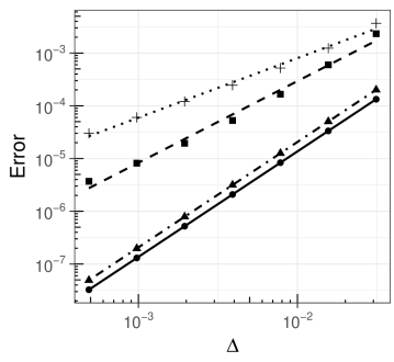
Figure 8: The computed errors for $E_{1}(\sigma_{h}h_{x})$ $({\color[rgb]{0,0,0}\bullet})$, $E_{\infty}(\sigma_{h}h_{x})$ $({\color[rgb]{0,0,0}\blacktriangle})$, $E_{1}(h_{x})$ ( $\blacksquare$ ), and $E_{\infty}(h_{x})$ $({\color[rgb]{0,0,0}+})$. The order of convergence for $\sigma_{h}h_{x}$ for both $E_{1}$ ( ) and $E_{\infty}$ (     ) errors is $2$, and the order of convergence for $h_{x}$ for $E_{1}$ (   ) and $E_{\infty}$ (     ) errors is $1.55$ and $1.13$, respectively. The symbols represent the errors from the computations and the lines show the linear fits.

We initialize the surface tension, $\sigma$, directly as a function of $x$, i.e. $\sigma\left(h\right)=1+\sigma_{h}(\tilde{h_{0}}+\varepsilon\cos(2\pi x))$. Figure 8 shows the convergence of the computed $\sigma_{h}h_{x}$ as a function of mesh refinement. As shown, the order of convergence is $2$ for both $E_{1}$ and $E_{\infty}$ errors. In this test case, the interfacial value of the surface tension $\tilde{\sigma}^{y}$ is computed in the $y$ direction for all cells. Figure 8 also shows the order of convergence of $h_{x}$, computed using height functions (see A.1), that is $1.55$ and $1.13$ for $E_{1}$ and $E_{\infty}$ errors, respectively. The lower order of convergence is contributed to the errors in initializing the volume fractions, and their convergence to the prescribed initial condition.

Next we investigate the accuracy of the computed surface gradient

$$\nabla_{s}\sigma\left(\mathbf{x}\right)=(\nabla_{s}\sigma)_{x}\,\hat{i}+(\nabla_{s}\sigma)_{y}\,\hat{j},$$

where $\left((\nabla_{s}\sigma)_{x},(\nabla_{s}\sigma)_{x}\right)=\left(G_{x}|t_{x}|,G_{y}|t_{y}|\right)$. Figure 9 compares the $x$ and $y$ components of the surface gradient with the exact solution. As shown, the $x$ component converges with order $1.9$ and $1.5$ for $E_{1}$ and $E_{\infty}$ errors, respectively, and the $y$ component converges with order $1.7$ and $1.4$ for $E_{1}$ and $E_{\infty}$ errors, respectively. The difference in the order of convergence is due to the interface orientation being in the horizontal direction and the gradient being imposed in the $x$ direction. Hence, the columns are always constructed in the $y$ direction, and the derivative along the interface is computed as ${\partial\sigma}/{\partial s^{x}}$, which captures the gradient in the horizontal direction more accurately.

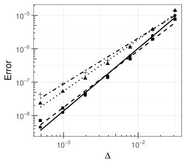
Figure 9: The computed errors for $E_{1}((\nabla_{s}\sigma)_{x})$ $({\color[rgb]{0,0,0}\bullet})$, $E_{\infty}((\nabla_{s}\sigma)_{x})$ $({\color[rgb]{0,0,0}\blacktriangle})$, $E_{1}((\nabla_{s}\sigma)_{y})$ ( $\blacksquare$ ), and $E_{\infty}((\nabla_{s}\sigma)_{y})$ $({\color[rgb]{0,0,0}+})$. The order of convergence for $(\nabla_{s}\sigma)_{x}$ is $1.9$ and $1.5$ for $E_{1}$ ( ) and $E_{\infty}$ (     ) errors respectively, and the order of convergence for $(\nabla_{s}\sigma)_{y}$ is $1.7$ and $1.4$ for $E_{1}$ (   ) and $E_{\infty}$ (     ) errors respectively. The symbols represent the errors from the computations and the lines show the linear fits.

Next we test the convergence for a more general interfacial geometry where the interfacial values of $\tilde{\sigma}^{c}$ are computed using columns in both $x$ and $y$ directions (see Section 3). We consider a circle of radius $a=0.25$ positioned at $(0.5,0.5)$ in a $1\times 1$ domain with an imposed temperature distribution

$$T(x,y)=\Delta T\left(x+y\right),$$ (47)

where $\Delta T$ is a constant. We assume that the thermal diffusivity is equal for the fluid inside and outside of the circle, i.e. $k_{1}=k_{2},C_{p1}=C_{p2},\rho_{1}=\rho_{2},\mu_{1}=\mu_{2},$ where the subscripts $1$ and $2$ denote surrounding and the fluid inside of the drop, respectively. Figure 10 shows the setup with color representing the temperature field. Here we choose $\Delta T=0.1$, $k_{1}=1$, $C_{p1}=1$ and $\rho_{1}=1$.

\begin{overpic}[width=173.44534pt]{temperature_sketch_xy.eps} \put(5.0,70.0){$\rho_{1},\mu_{1}$} \put(5.0,60.0){$k_{1},C_{p1}$} \put(60.0,45.0){$a$ } \end{overpic}

Figure 10: The initial setup of a circular drop with an imposed uniform temperature gradient. The color shows the temperature with dark blue and dark red being the minimum and maximum values respectively.

For simplicity, we assume that the surface tension is a linear function of temperature, i.e. $\sigma\left(T\right)=1+\sigma_{T}T,$ where we let $\sigma_{T}=-0.1$. We set the velocity to zero, and knowing that the interface is exactly circular, we can compute exact surface gradient from the definition

$$\nabla_{s}\sigma =\nabla\sigma-\hat{\mathbf{n}}\left(\hat{\mathbf{n}}\cdot\nabla\sigma\right),$$ (48)

$$=\frac{\sigma_{T}\Delta T}{a^{2}}\left\langle a^{2}-x^{2}\mp x\sqrt{a^{2}-x^{2}},x^{2}\mp x\sqrt{a^{2}-x^{2}}\right\rangle,$$ (49)

$$=\frac{\sigma_{T}\Delta T}{a^{2}}\left\langle y^{2}\mp y\sqrt{a^{2}-y^{2}},a^{2}-y^{2}\mp y\sqrt{a^{2}-y^{2}}\right\rangle$$ (50)

Equations (49) and (50) give the surface gradient as a function of $x$ and $y$, respectively.

We initialize the temperature following two approaches, and discuss their performance. First approach is to define the interface as a function of $x$ and $y$ depending on the more favorable interface orientation as follows

$$T(x,y)=\begin{cases}\Delta T\left(x\pm\sqrt{a^{2}-x^{2}}\right)&\mbox{if }|x|<|y|,\\ \Delta T\left(y\pm\sqrt{a^{2}-y^{2}}\right)&\mbox{otherwise},\end{cases}$$ (51)

where $x$ and $y$ are coordinates of the cell centers. Second approach is to use positions of the centroid of the interface contained in each cell to initialize the temperature by equation (47). We show below that the second approach leads to more accurate results.

We compare the computed surface gradient with the exact solution by considering $E_{1}$ and $E_{\infty}$ errors defined in equations (45) and (46), respectively. Similarly as in the previous example, in order to eliminate the dependence of the errors on the interface position in the cell, the center of the drop is positioned randomly in the interval $[0,\Delta]\times[0,\Delta]$, and the errors are averaged over $100$ random realizations. Figure 11 shows the convergence to the exact solution for the $x$ and $y$ components of the gradient. The convergence of $E_{1}$ error is $0.85$ and $0.86$ for the $x$ and $y$ components, respectively.

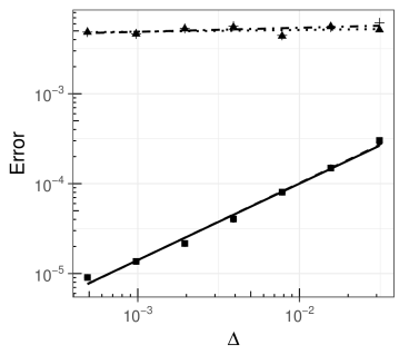
Figure 11: The computed error for $E_{1}((\nabla_{s}\sigma)_{x})$ $({\color[rgb]{0,0,0}\bullet})$, $E_{\infty}((\nabla_{s}\sigma)_{x})$ $({\color[rgb]{0,0,0}\blacktriangle})$, $E_{1}((\nabla_{s}\sigma)_{y})$ ( $\blacksquare$ ), and $E_{\infty}((\nabla_{s}\sigma)_{y})$ $({\color[rgb]{0,0,0}+})$. The order of convergence for $(\nabla_{s}\sigma)_{x}$ is $0.85$ and $0.019$ $E_{1}$ ( ) and $E_{\infty}$ (     ) errors respectively, and the order of convergence for $(\nabla_{s}\sigma)_{y}$ is $0.86$ and $0.045$ for $E_{1}$ (   ) and $E_{\infty}$ (     ) errors, respectively. The symbols represent the errors from the computations, and the lines show the linear fit of those points.

The slow convergence of $E_{\infty}$ error is due to the errors in initializing the temperature at the lines $|x|=|y|$ from equation (51), demonstrated later.

In order to reduce the influence of the initialization of $T$ on the convergence, we also compute the convergence of $L_{1}$ norm of each component of the surface gradient

$$L_{1}\left(f\right)=\frac{1}{N}\sum_{i}^{N}|f_{i}|,$$ (52)

where $f_{i}$ is the $x$ or $y$ component of the surface gradient, and $N$ is the number of interfacial points.

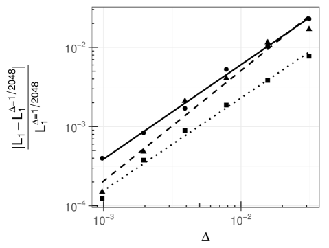
Figure 12: The computed errors for $L_{1}((\nabla_{s}\sigma)_{x})$ $({\color[rgb]{0,0,0}\bullet})$, $L_{1}((\nabla_{s}\sigma)_{y})$ $({\color[rgb]{0,0,0}\blacktriangle})$, and $L_{1}(T)$ ( $\blacksquare$ ). The order of convergence for $(\nabla_{s}\sigma)_{x}$ and $(\nabla_{s}\sigma)_{y}$ is $1.2$ ( ) and $1.4$ (   ), respectively. The order of convergence of $T(x,y)$ at the interface is $1.2$ (     ). The symbols represent the errors from the computations and the lines show the linear fit of those points.

Figure 12 shows $L_{1}$ norm for the $x$ and $y$ components of the surface gradient and the order of convergence of the temperature $T(x,y)$ in the interfacial points as a function of the mesh size, $\Delta$. We find the order of convergence of the $x$ and $y$ components of the surface gradient to be $1.2$ and $1.4$. The order of convergence of $T(x,y)$ along the interface is $1.2$. This indicates that the order of convergence of the surface gradient is limited by the order of convergence of the initial temperature at the interface.

Figure 13(a) shows the distribution of errors at the circular interface for one random realization. The largest errors appear around the lines $|x|=|y|$. Based on this we conclude that the lack of convergence of $E_{\infty}$ error is caused by the initialization of the temperature which changes the dependence on $x$ or $y$ variable at the lines $|x|=|y|$.

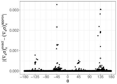
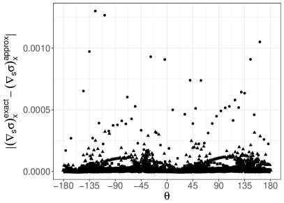
(a)                                                    (b)

Figure 13: Errors of the $x$ component of the surface gradient at the interfacial cells for $\Delta=a/8$ $({\color[rgb]{0,0,0}\bullet})$, $a/32$ $({\color[rgb]{0,0,0}\blacktriangle})$, $a/128$ ( $\blacksquare$ ), and $a/512$ $({\color[rgb]{0,0,0}+})$. Initializing the temperature using (a) equation (51) and (b) equation (53). $\theta$ is defined to be zero at the positive $x$ axis and increasing counterclockwise.

In order to initialize the temperature more accurately at the interface we use the centroid of the interface segment contained in each cell, $(x_{c},y_{c})$. Then the initial temperature is given by

$$T(x,y)=\Delta T\left(x_{c}+y_{c}\right).$$ (53)

This reduces the errors from initializing the temperature at the lines $|x|=|y|$ compared to using equation (51). Here, we also explore a different way of approximating interfacial temperature, and use surface area weighted average instead of volume fraction weighted average (see Section 3). The volume weighted average gives the temperature at the center of the mass of the fluid phase in the column, whereas the surface area weighted average gives the temperature at the center of the interface in the column. Hence, the latter is consistent with the initialization of the temperature using equation (53).

Figure 13(b) shows the errors of the $x$ component of the surface gradient at the interfacial cells if the temperature is initialized using equation (53). The errors are still largest around $|x|=|y|$, however those are the usual “weak” spots of the height function construction. Figure 14 shows the improvement in the convergence to the exact solution using $L_{1}$ and $L_{\infty}$ norm for the $x$ and $y$ components of the surface gradient as a function of mesh refinement. The order of convergence for $L_{1}$ norm is $0.94$ and $0.89$ for the $x$ and $y$ components of the surface gradient, respectively, and the order of convergence for $L_{\infty}$ norm is $0.65$ and $0.58$ for the $x$ and $y$ components of the surface gradient, respectively. Hence, the second approach of initializing the temperature (using equation (53)) improves the convergence of the $L_{\infty}$ norm significantly.

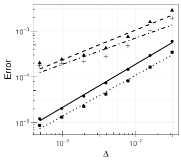
Figure 14: The computed errors for $E_{1}((\nabla_{s}\sigma)_{x})$ $({\color[rgb]{0,0,0}\bullet})$, $E_{\infty}((\nabla_{s}\sigma)_{x})$ $({\color[rgb]{0,0,0}\blacktriangle})$, $E_{1}((\nabla_{s}\sigma)_{y})$ ( $\blacksquare$ ), and $E_{\infty}((\nabla_{s}\sigma)_{y})$ $({\color[rgb]{0,0,0}+})$. The order of convergence for for $(\nabla_{s}\sigma)_{x}$ is $0.94$ ( ) and $0.65$ (   ) for $E_{1}$ and $E_{\infty}$ errors, respectively, and the order of convergence for for $(\nabla_{s}\sigma)_{y}$ is $0.89$ (     ) and $0.58$ (     ), respectively. The symbols represent the errors from the computations, and the lines show the linear fit of those points.

4.2 Drop migration

We further test our numerical implementation using a classical problem of the thermocapillary drop migration (see the reviews [4, 31]). A drop or a bubble placed in a fluid with an imposed temperature gradient moves due to the variation in the surface tension as a function of temperature. Several authors use this problem for benchmarking their numerical algorithms for a temperature dependent surface tension [19, 32, 33]. We show the comparison of our numerical results with the available work in the literature. We also show the comparison with the analytical solution of the drop terminal velocity by Young et al. [34]. Young et al. [34] show that the nondimensional velocity of the drop in an unbounded domain for an axysimmetric geometry in the limit of small Ma and Ca numbers can be approximated as

$$v^{*}_{ygb}=\frac{\mu_{1}}{\sigma_{T}a\Delta T}\frac{2}{(2+k_{r})(2+3\mu_{r})},$$ (54)

where $\mu_{1}$ is the viscosity of the surrounding fluid, $\sigma_{T}$ is the (constant) gradient of the surface tension with respect to the temperature, $a$ is the drop/bubble radius, $\Delta T$ is the imposed temperature gradient, and $k_{r}$ and $\mu_{r}$ are the thermal conductivity and viscosity ratios, respectively, for the drop/bubble compared to the surrounding fluid.

\begin{overpic}[width=195.12767pt]{temperature_sketch_new.eps} \put(40.0,3.0){\color[rgb]{1,1,1}$T^{*}=T^{*}_{1}$} \put(39.0,93.0){\color[rgb]{1,1,1}$T^{*}=T^{*}_{2}$} \put(5.0,60.0){$\rho_{1},\mu_{1}$} \put(5.0,50.0){$k_{1},C_{p_{1}}$} \put(60.0,45.0){$a$ } \end{overpic}

Figure 15: The initial setup of the drop migration problem. The color represents the linear temperature distribution with imposed temperatures $T^{*}_{1}$ and $T^{*}_{2}$ at the horizontal boundaries.

Figure 15 shows the considered setup: a drop or a bubble of radius $a$ is placed in an ambient fluid, with a linear temperature gradient imposed in the $y$ direction. The temperature at the top and the bottom boundaries is set to constant values and a zero heat flux boundary condition is imposed at the left and right boundaries. The boundary conditions for the flow are no-slip and no penetration at the top and bottom boundaries and symmetry at the left and right boundaries.

We solve equations (10) and (15) and consider the following scales

$$p_{0}=\frac{\mu_{1}U_{0}}{a},\,\,\,\,\,t_{r}=\frac{a}{U_{0}},\,\,\,\,\,U_{0}=\frac{\sigma_{T}a\Delta T}{\mu_{1}}\,\,\,\,\,T_{0}=a\Delta T,$$

where the subscript $1$ denotes the properties of the ambient fluid. The surface tension at the interface between the drop and the ambient fluid is assumed to depend linearly on temperature as given by equation (20), which rescaled using the scales above yields

$$\sigma^{*}=1+\text{Ca}\left(T^{*}-T_{R}^{*}\right).$$ (55)

Next we present the comparison of our results with the available studies in the literature.

We start by comparing our results with the ones by Ma and Bothe [19]. The material properties are $\rho_{1}=500\frac{kg}{m^{3}},\,\mu_{1}=0.024\,Pa\cdot s,\,\sigma_{0}=10^{-2}\frac{N}{m},\,\sigma_{T}=2\times 10^{-3}\frac{N}{mK},\,k_{1}=2.4\times 10^{-6}\frac{W}{mK},\,C_{p_{1}}=10^{-4}\frac{J}{kgK},\,\Delta T=200\frac{K}{m},\,T_{2}=290\,K,\,a=1.44\times 10^{-3}\,m.$ The ratio of the material properties between the ambient fluid and the drop is $2$. These physical properties give nondimensional parameters $\text{Re}=\text{Ma}=0.72,\,\text{Ca}=0.0576$, and the velocity scale $U_{0}=0.024\,\frac{m}{s}$. Figure 16 shows the computed velocity field in the drop and the surrounding fluid. The surface tension gradient drives the flow from low surface tension region (top) to high surface tension region (bottom). This creates the flow inside the drop and as a result the drop moves in the positive $y$ direction. The drop velocity is computed using the following definition of the centroid velocity

$$v_{c}^{*}=\frac{\sum\limits_{i,j}v^{*}_{i,j}\chi_{i,j}\,(\Delta_{i,j}^{*})^{2}}{\sum\limits_{i,j}\chi_{ij}\,(\Delta_{i,j}^{*})^{2}}$$

where $v^{*}_{i,j}$ is the $y$ component of the cell-center velocity.

Figure 16: The velocity field in the drop and the surrounding fluid.

Figure 17 shows the computed velocity of the drop compared to the results in Ma and Bothe [19]. In this test case, the computational domain is a square box with a side length equal to four times the drop radius; the drop is initially placed at the center of the domain. As shown, our results are in agreement with the previously obtained simulations in Ma and Bothe [19].

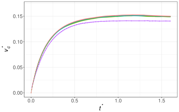
Figure 17: Drop migration velocity for $\text{Re}=\text{Ma}=0.72$ and $\text{Ca}=0.0576$ for $\Delta=$ $1/64$ ( ), $1/256$ ( ), and $1/256$ ( ) compared with the result given in [19] ( ) for 2D simulations.

Next, we carry out another comparison for smaller value of Re and Ca numbers and when $\text{Ma}=0$; we choose $\text{Re}=\text{Ca}=0.066$ in accordance with the results presented in [33] for the VOF method. The computational box is a rectangle of size $10a\times 15a$. The density of the ambient fluid is set to $\rho_{1}^{*}=0.2$, and viscosity is $\mu_{1}^{*}=0.1$. The ratio of the physical properties of the drop to the ambient fluid is set to $1$. The surface tension is $\sigma_{0}^{*}=0.1$ at the reference temperature $T_{R}^{*}=0$, with $\sigma_{T}^{*}=-0.1$. The temperature gradient is set to $\Delta T^{*}=0.1\bar{3}$, which is fixed by setting $T_{1}^{*}$ = 0 and $T_{2}^{*}=1$. The drop is initially centered horizontally at $3a$ from the bottom wall. Figure 18 shows the comparison of our method with the results in [33], along with temporal convergence of our method. Compared to the results by Herrmann et al. [33], our results do not exhibit oscillations, which agrees with the asymptotic solution of constant rise velocity. Another difference is that our terminal velocity converges to a smaller value with decreasing time step. However, the timestep used in the results of Herrmann et al. [33] is not specified in their paper.

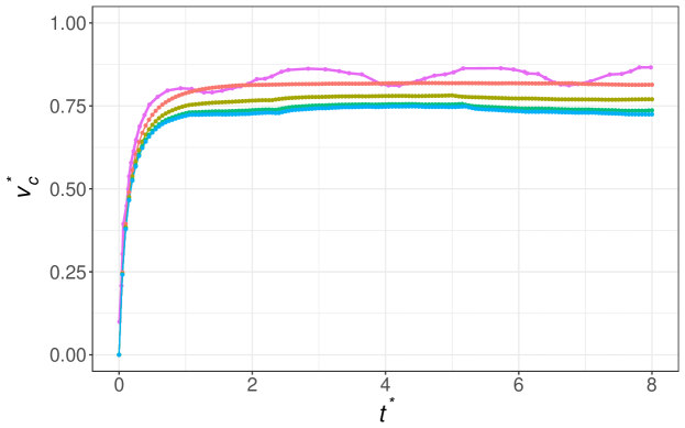
Figure 18: Convergence of the migration velocity as a function of the time step for $\Delta t=$ $10^{-4}$ ( ), $5\times 10^{-6}$ ( ), $10^{-5}$ ( ), and $5\times 10^{-6}$ ( ) compared with the results in the results[33] ( ) for 2D simulation, for $\text{Re}=\text{Ca}=0.066$ and $\text{Ma}=0$. The velocity is rescaled by $v^{*}_{ygb}$.

We also test the convergence to the analytical solution obtained in the limit of Ma and Re approaching zero and in the unbounded domain, where the terminal velocity approaches $v^{*}_{ygb}$ value given in equation (54). Figure 19 shows the terminal velocity of a droplet for a 2D simulation as a function of a distance from the wall for $\text{Re}=\text{Ma}=2.5\times 10^{-3}$ and $\text{Ca}=1.25\times 10^{-3}$. The terminal velocity converges to a value lower than $v^{*}_{ygb}$ due to the difference in the geometry. We next show that our 3D result in fact converges to this analytical solution.

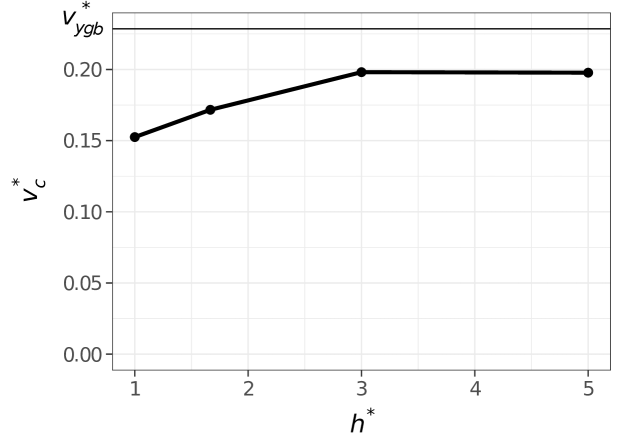
Figure 19: Convergence of the terminal velocity with increased distance from the wall, $h^{*}$, for $\text{Re}=\text{Ma}=2.5\times 10^{-3}$ and $\text{Ca}=1.25\times 10^{-3}$ for 2D simulations.

We perform similar tests for the 3D simulations. Figure 20 shows the migration velocity for $\text{Re}=\text{Ma}=0.72$ and $\text{Ca}=0.0576$. The parameters and the domain size are equivalent to the simulation results shown in Figure 17. The results also show that the oscillations in the computed velocity decay with mesh refinement and the terminal velocity converges to a higher value compared to the 2D case. However, this value is still smaller than $v^{*}_{ygb}$ due to the small domain size and relatively large Re and Ma numbers.

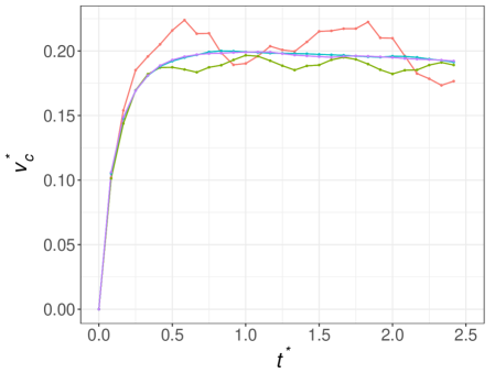
Figure 20: Convergence of the migration velocity in a 3D simulation with mesh refinement for $\Delta=$ $1/16$ (  ), $1/32$ ( ), and $1/64$ ( ), and $1/128$ ( ); $\text{Re}=\text{Ma}=0.72$ and $\text{Ca}=0.0576$.

Figure 21 shows the terminal velocity of a droplet for a 3D simulation as a function of a distance from the wall for $\text{Re}=\text{Ma}=2.5\times 10^{-3}$ and $\text{Ca}=10^{-3}$. As shown, the terminal velocity approaches the analytical value $v^{*}_{ygb}$.

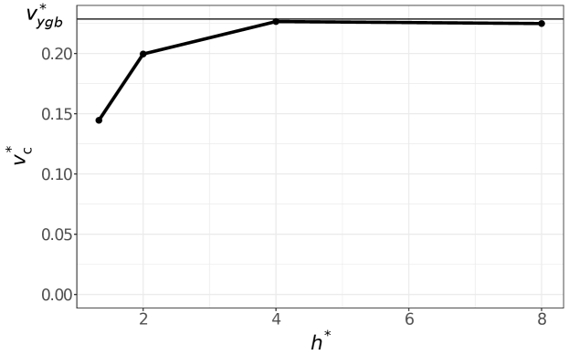
Figure 21: Convergence of the terminal velocity with increased distance from the wall, $h^{*}$, for $\text{Re}=\text{Ma}=2.5\times 10^{-3}$ and $\text{Ca}=10^{-3}$ for 3D simulations.

In this section we have shown the comparison of our method with existing literature and with a limiting analytical solution. Our method shows the convergence to the analytical value of the terminal velocity. Furthermore, the trend of the solution as well as the time needed to reach the terminal velocity are consistent with the previously reported results.

4.3 Coalescence and non-coalescence of sessile drops

Next we demonstrate the performance of our numerical methods through an example of the coalescence behavior of sessile drops with different surface tension. We model the experiments of the coalescence of two droplets with different alcohol concentrations by Karpitschka et. al. [35, 36, 37]. In their experimental study, they show three coalescence regimes depending on the surface tension difference between the two droplets: immediate coalescence, delayed coalescence, and non-coalescence. They identify a key parameter that governs the transition between the delayed and non-coalescence regimes: specific Marangoni number M $=3\Delta\sigma/(2{\bar{\sigma}}\theta^{2})$ [37], where $\Delta\sigma$ is the difference in the surface tension between the two drops and ${\bar{\sigma}}$ is the average of the surface tension of two drops. They determine a threshold Marangoni number M${}_{t}\approx 2\pm 0.2$ experimentally for the transition between the delayed coalescence and non-coalescence regimes.

Here we show that our numerical simulations also reveal the three regimes in agreement with the experimental observations in [35, 36]. From the numerical simulation point of view, this problem involves a level of difficulty: unlike temperature, the concentration should remain strictly confined to the liquid phase and should not leak out to the ambient phase. To avoid this difficulty, we combine our variable surface tension methodology with the numerical technique already implemented in the original version of gerris[28] which prevents the concentration from leaking out of the liquid domain into the ambient phase.

Figure 22: A schematic of the drop coalescence problem.

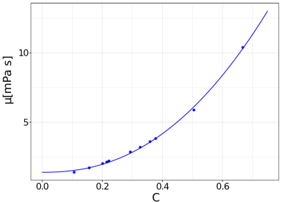
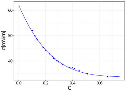
(a)                                               (b)

Figure 23: Viscosity (a) and surface tension (a) of the mixture of 1,2-Butanediol and water as a function of alcohol concentration. Points represent the data from Karpitschka and Riegler [35], and the lines show the fit of the points.

We model the 2D problem since the dominant flow dynamics in the problem is in the region connecting the two droplets, where the surface tension gradient is the strongest, and in this region we can ignore the out of plane curvatures. Initially, the drops have the shape of a circular segment with the base radius $R_{b}$ and a contact angle $\theta$, and are connected by an overlap of $0.25R_{b}$ (see Figure 22). The drops have equal base radius $R_{b}$ and we assume that their densities are equal. The viscosity depends on the alcohol concentration $C$, where we use a nonlinear fit to the data given in [35] of the form

$$\mu\left(C\right)=\mu_{1}+a_{\mu}\left(\mu_{2}-\mu_{1}\right)\left(1-C\right)^{n_{\mu}},$$ (56)

shown in Figure 23(a). Drops are composed of the mixture of the 1,2-Butanediol and water, but they differ in the concentrations of alcohol. Figure 23(b) shows the surface tension dependence on the concentration of 1,2-Butanediol in water. Similarly as for the viscosity, we fit this data to a function of the form

$$\sigma\left(C\right)=\sigma_{1}+a_{\sigma}\left(\sigma_{2}-\sigma_{1}\right)\left(1-C\right)^{n_{\sigma}},$$ (57)

Parameters $a$ and $n$ are determined from the fit.

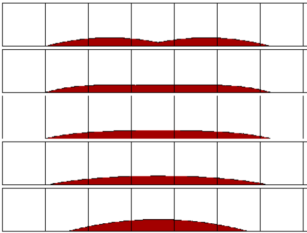
Figure 24: Evolution of two drops with equal alcohol concentration, i.e. no surface tension difference, at times $t=0\,s$, $t=0.02\,s$, $t=0.04\,s$, $t=0.1\,s$ and $t=1\,s$ from top to bottom. The color shows the concentration of alcohol. Each box is equivalent to $2\,mm$.

We first show a simulation of two drops, with equal surface tension. We consider the case where the concentration of alcohol is $45$%, and the base radii of the circular segments are both $R_{b}=3\,mm$. Along with a no-slip boundary condition at the substrate, we also impose a $\theta=15^{\circ}$ contact angle. For the contact angle implementation in gerris and related numerical discussion the reader is referred to [29, 38]. Figure 24 shows the evolution of the interface at different times. The droplets coalesce immediately, fully merge after $0.1\,s$, and assume an equilibrium shape of one large circular segment at a later time. The color represents the concentration of alcohol, which is contained inside of the fluid and zero in the surrounding.

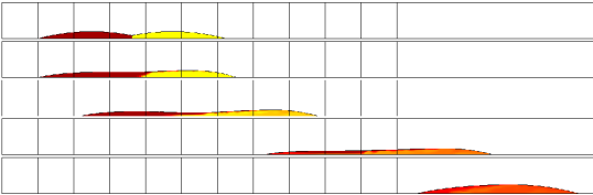
Figure 25: Evolution of two drops with small surface tension difference at times $t=0\,s$, $t=0.1\,s$, $t=1\,s$, $t=5\,s$, and $t=10\,s$ from top to bottom. The color shows the concentration of alcohol. Each box is equivalent to $2\,mm$.

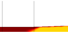
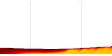
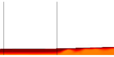
Figure 26: Closeup of the neck region between the two drops shown in Figure 25, at times $t=0.1,\ s$, $t=1\,s$, and $t=5,\ s$ from left to right. The color shows the concentration of alcohol.

Next we examine the case where $\text{M}\approx 1.2<\text{M}_{t}$. Figure 25 shows the simulations of this intermediate regime where droplets coalescence is delayed. Here, we set drop $1$ to $45$% and drop $2$ to $35$% of alcohol. The connected drops move toward higher surface tension due to the Marangoni induced flow until the concentrations are mixed, resulting in a smaller gradient in the surface tension. Figure 26 shows closeup images of the neck region between the two drops corresponding to the three panels in the middle shown in Figure 25. In this figure, we show the flow mixing dynamics which leads to the decrease of the surface tension difference in the neck region, resulting in a consequent full coalescence of the two drops.

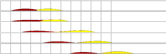
Figure 27: Non-coalescence of drops at times $t=0\,s$, $t=0.1\,s$, $t=1\,s$, $t=2\,s$, and $t=6\,s$ from top to bottom. The color shows the concentration of alcohol. Each box is equivalent to $2\,mm$.

Figure 28: Closeup of the neck region between the two drops shown in Figure 27, at times $t=0.1\,s$, $t=1\,s$, and $t=2\,s$ from left to right. The color shows the concentration of alcohol.

Next we consider a case in the non-coalescence regime. We set drop $1$ to $45$% and drop $2$ to $33$% of alcohol. Figure 27 shows the simulation results for $\text{M}\approx 1.8\approx\text{M}_{t}$. In this case, the Marangoni induced flow initially pushes the fluid from drop $1$ towards drop $2$. However, this results in the thinning of the connecting neck between the drops (at $t=1\,s$), and the fluid cannot pass from drop $1$ to drop $2$ anymore. Figure 28 shows closeup images of the neck region between the two drops corresponding to the middle three panels shown in Figure 27. Compared to the previous case where droplets coalescence is delayed (M $\approx 1.2$), the behavior of the mixing of the fluids in the neck region is prevented by the thinning of the neck. Hence these droplets do not coalesce, but instead they move together with a constant velocity $u_{d}$ on the substrate in the direction of the higher surface gradient.

This quasi-steady behavior is also observed in the experiments by Karpitschka and Riegler [36]. Figure 29(a) shows the velocity of the points at the interface after the quasi-steady state is reached as a function of the distance from the bridge region, $D_{b}$. The points to the left of the bridge region have a velocity $\approx 2u_{d}$ (solid line). At the bridge region the interface is close to the solid substrate and the velocity becomes close to zero due to the no-slip boundary condition. In the region close to the bridge in drop $2$, the velocity has a jump and reaches the maximum value due to the Marangoni effect resulting from a high surface tension gradient at the neck region. Away from the bridge, the velocity is again comparable to $u_{d}$. This behavior is in qualitative agreement with the experimental observation by Karpitschka and Riegler [36, 37]. To provide more insight into the flow through the neck region, in Figure 29(b) we present the alcohol concentration at the interface as a function of the distance from the bridge region, $D_{b}$. As shown, a localized and steady state surface tension gradient is established through the neck region. This Marangoni effect can counteract the capillary effect that would otherwise result in the coalescence and can therefore sustain the non-coalescence and the movement of drops temporarily.

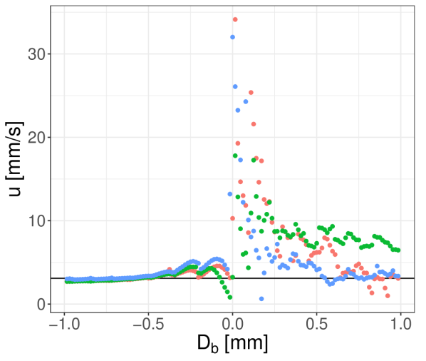
(a)

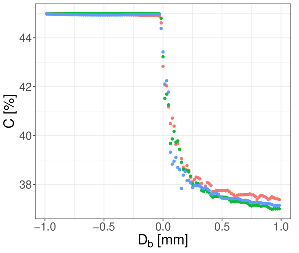
(b)

Figure 29: The $x$ component of the velocity field at the interface interfacial points (a) and the concentration of alcohol at the interfacial points (b) for the non-coalescent drops for the example shown in Figure 27. The color shows different times, with red, green and blue being $t=4\,s$, $t=5\,s$, and $t=6\,s$, respectively.

5 Conclusions

We have developed a new numerical methodology for including variable surface tension in a VOF based Navier-Stokes solver. The method handles both temperature or concentration dependent surface tension variations. We employ a height function inspired formulation to compute surface gradients and the resulting stresses at the interface (Marangoni forces) in a more general numerical framework. We show the robustness and accuracy of our developed method by studying the convergence of the computation of the surface gradient for multiple geometries and the convergence of the terminal velocity for the classical problem of the drop migration with an imposed constant temperature gradient. The drop migration simulation results are in agreement with the available theoretical and numerical results. We also show that our method produces results consistent with experimental data in the case of concentration dependent surface tension. Our numerical implementation extends to adaptively refined meshes which improves the computational efficiency for Marangoni induced flows that require a high resolution around the interface.

The presented approach represents a first attempt for implementing a general variable surface tension in the VOF method. As presented here, our method can subsequently be used directly for surface tension dependence on the surfactant concentration. This includes implementing the solution to the surfactant transport equation for soluble and insoluble surfactants. Our methodology can provide tools for developing more robust and accurate numerical simulations for two-phase flows with surfactants. Surfactant flows have many applications, e.g. in chemical industry, pharmaceuticals and technology [39], and their understanding will have far reaching effects in many areas.

The numerical verifications and validations with available literature demonstrate the efficiency and applicability of our methodology. Our numerical approach is implemented in an adaptive mesh refinement framework, which now makes detailed numerical simulations that incorporate the effects of tangential (Marangoni) stresses feasible. This is particularly relevant for a number of flow problems where Marangoni effect may play a crucial role, such as the evolution of thin films on nanoscale, where Marangoni effects may result either from concentration gradients (mixture of two fluids) or thermal gradients due to internal or external sources. Our future research will continue in this direction.

Appendix A Appendix

A.1 Height functions

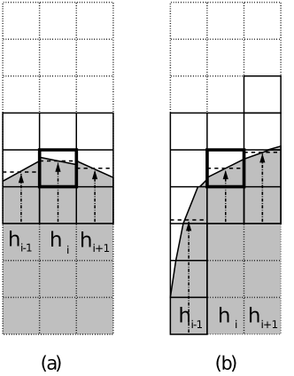
Figure 30: Height function computation with compact stencil constructed independently for each column. (a) Stencil for a slightly curved interface. (b) Asymmetric stencil, where each column requires different number of cells. From [23].

An accurate computation of interface normals and curvature in the VOF method can be achieved using the height function method [40]. In this method, height functions are defined in each interfacial cell as a sum of the volume fractions in fluid column constructed of interfacial cells in vertical or horizontal orientation. Figure 30 shows columns with vertical orientation used for calculating height functions implemented in Gerris solver [23]; the solid lines show the stencil size required to calculate the curvature in the cell marked by the bold lines. The height function for the the column $i$ is

$$h_{i}=\sum\limits_{k}\chi_{i,k},$$ (58)

where the index $k$ includes all interfacial cells in the columns. The number of cells used for construction of the columns is optimized based on the each column, i.e. there is no fixed stencil size, as illustrated in Figure 30. Figure 30(a) shows a symmetric stencil where only three cells are required for calculating height function in each column. Figure 30(b) shows an asymmetric stencil where each column requires including different number of cells.

In 2D, the height function can be calculated in either $x$ or $y$ direction, depending on the orientation of the interface. Here, we will present the discretization for height function for columns in the $y$ direction (as in Figure 30). For heights collected in the $x$ direction the equations are equivalent with derivatives of height function with respect to $x$ replaced by the derivatives with respect to $y$. The curvature of the interface is calculated from the height functions as

$$\kappa=\frac{h_{xx}}{\left(1+h_{x}^{2}\right)^{3/2}},$$ (59)

where the derivatives of the height functions in equation (59) are calculated using a second order central difference

$$h_{x}=\frac{h_{i+1}-h_{i-1}}{2\Delta},$$ (60)

$$h_{xx}=\frac{h_{i+1}-2h_{i}+h_{i-1}}{\Delta^{2}},$$ (61)

where $\Delta$ is the cell size. In 3D, e.g. if the columns are computed in $z$ direction, the curvature is

$$\kappa=\frac{h_{xx}+h_{yy}+h_{xx}h_{y}^{2}+h_{yy}h_{x}^{2}-2h_{xy}h_{x}h_{y}}{\left(1+h_{x}^{2}+h_{y}^{2}\right)^{3/2}}.$$ (62)

A.2 Algorithm

Algorithm 1 shows the pseudocode for approximating the interfacial value of the surface tension $\tilde{\sigma}$ in each column.

for Each component $c\in\{x,y,z\}\equiv\{0,1,2\}$  do

       for All interfacial cells $\mathcal{C}$ do

             Set $V\leftarrow\chi\left(\mathcal{C}\right)$, $\tilde{\sigma}^{c}\leftarrow V\sigma\left(\mathcal{C}\right)$;

             for Each direction $d\in\{2c,2c+1\}$ do

                   Set $\mathcal{N}\leftarrow$ neighboring cell of $\mathcal{C}$ in direction $d$;

                   while $0<\chi\left(\mathcal{N}\right)<1$ do

                         Set $v_{d}\leftarrow\chi\left(\mathcal{C}\right)$, $\tilde{\sigma}^{c}\leftarrow\tilde{\sigma}^{c}+v_{d}\sigma\left(\mathcal{N}\right)$, $V\leftarrow V+v_{d}$ ;

                         Set $\mathcal{N}\leftarrow$ neighboring cell of $\mathcal{N}$ in direction $d$;

                        

                   end while

                  

             end for

            if  $\{v_{2c},v_{2c+1}\}\supset\{0,1\}$  then

                   Set $\tilde{\sigma}^{c}\left(\mathcal{C}\right)\leftarrow\tilde{\sigma}^{c}/V$;

                  

            else

                   Return inconsistent $\tilde{\sigma}^{c}\left(\mathcal{C}\right)$ ;

                  

             end if

            

       end for

      

end for

Algorithm 1 Defining interfacial values $\tilde{\sigma}$ for each column direction.

References

- Scriven and Sternling [1960] L. E. Scriven, C. V. Sternling, The Marangoni effects, Nature 187 (1960) 186–188.
- Farahi et al. [2004] R. H. Farahi, A. Passian, T. L. Ferrell, T. Thundat, Microfluidic manipulation via Marangoni forces, Appl. Phys. Lett. 85 (2004) 4237–4239.
- Kundan et al. [2015] A. Kundan, J. L. Plawsky, P. C. Wayner, D. F. Chao, R. J. Sicker, B. J. Motil, T. Lorik, L. Chestney, J. Eustace, J. Zoldak, Thermocapillary phenomena and performance limitations of a wickless heat pipe in microgravity, Phys. Rev. Lett. 114 (2015) 146105–5.
- Subramanian et al. [2002] R. S. Subramanian, R. Balasubramaniam, G. Wozniak, Fluid mechanics of bubbles and drops, in: R. Monti (Ed.), Physics of Fluids in Microgravity, Taylor and Francis, 2002, pp. 149–177.
- Trice et al. [2008] J. Trice, D. Thomas, C. Favazza, R. Sureshkumar, R. Kalyanaraman, Novel Self-Organization Mechanism in Ultrathin Liquid Films: Theory and Experiment, Phys. Rev. Lett. 101 (2008) 017802–4.
- Dong and Kondic [2016] N. Dong, L. Kondic, Instability of nanometric fluid films on a thermally conductive substrate, Phys. Rev. Fluids 1 (2016) 063901–16.
- Davis [1987] S. Davis, Thermocapillary instabilities, Ann. Rev. Fluid Mech. 19 (1987) 403–435.
- Craster and Matar [2009] R. Craster, O. Matar, Dynamics and stability of thin liquid films, Rev. Mod. Phys. 81 (2009) 1131–1198.
- Muradoglu and Tryggvason [2014] M. Muradoglu, G. Tryggvason, Simulations of soluble surfactants in 3D multiphase flow, J. Comput. Phys. 274 (2014) 737–757.
- Xu et al. [2006] J.-J. Xu, Z. Li, J. Lowengrub, H. Zhao, A level-set method for interfacial flows with surfactant, J. Comput. Phys. 212 (2006) 590–616.
- Teigen et al. [2011] K. E. Teigen, P. Song, J. Lowengrub, A. Voigt, A diffuse-interface method for two-phase flows with soluble surfactants, J. Comput. Phys. 230 (2011) 375 – 393.
- Blanchette et al. [2009] F. Blanchette, L. Messio, J. W. M. Bush, The influence of surface tension gradients on drop coalescence, Phys. Fluids 21 (2009) 072107–10.
- Blanchette and Shapiro [2012] F. Blanchette, A. M. Shapiro, Drops settling in sharp stratification with and without Marangoni effects, Phys. Fluids 24 (2012) 042104–17.
- Lai et al. [2008] M.-C. Lai, Y.-H. Tseng, H. Huang, An immersed boundary method for interfacial flows with insoluble surfactant, J. Comput. Phys. 227 (2008) 7279–7293.
- Booty and Siegel [2010] M. R. Booty, M. Siegel, A hybrid numerical method for interfacial fluid flow with soluble surfactant, J. Comput. Phys. 229 (2010) 3864–3883.
- Schranner and Adams [2016] F. S. Schranner, N. A. Adams, A conservative interface-interaction model with insoluble surfactant, J. Comput. Phys. 327 (2016) 653–677.
- Drumright-Clarke and Renardy [2004] M. A. Drumright-Clarke, Y. Renardy, The effect of insoluble surfactant at dilute concentration on drop breakup under shear with inertia, Phys. Fluids 16 (2004) 14–21.
- James and Lowengrub [2004] A. J. James, J. Lowengrub, A surfactant-conserving volume-of-fluid method for interfacial flows with insoluble surfactant, J. Comput. Phys. 201 (2004) 685–722.
- Ma and Bothe [2011] C. Ma, D. Bothe, Direct numerical simulation of thermocapillary flow based on the Volume of Fluid method, Int. J. Multiphase Flow 37 (2011) 1045–1058.
- Francois and Swartz [2010] M. M. Francois, B. K. Swartz, Interface curvature via volume fractions, heights, and mean values on nonuniform rectangular grids, J. Comput. Phys. 229 (2010) 527–540.
- López and Hernández [2010] J. López, J. Hernández, On reducing interface curvature computation errors in the height function technique, J. Comput. Phys. 229 (2010) 4855–4868.
- Alexeev et al. [2005] A. Alexeev, T. Gambaryan-Roisman, P. Stephan, Marangoni convection and heat transfer in thin liquid films on heated walls with topography: Experiments and numerical study, Phys. Fluids 17 (2005) 062106–13.
- Popinet [2009] S. Popinet, An accurate adaptive solver for surface-tension-driven interfacial flows, J. Comput. Phys. 228 (2009) 5838–5866.
- Popinet [2003] S. Popinet, Gerris: a tree-based adaptive solver for the incompressible Euler equations in complex geometries, J. Comput. Phys. 190 (2003) 572–600.
- Brackbill et al. [1992] J. U. Brackbill, D. B. Kothe, C. Zemach, A continuum method for modeling surface tension, J. Comput. Phys. 100 (1992) 335–354.
- Landau and Lifshitz [1987] L. D. Landau, E. M. Lifshitz, Fluid mechanics, 2nd, volume 6, Pergamon Press, Oxford, 1987.
- Levich and Krylov [1969] V. G. Levich, V. S. Krylov, Surface-tension-driven phenomena, Annu. Rev. Fluid Mech. 1 (1969) 293–316.
- Popinet [1999] S. Popinet, Gerris Flow Solver, 1999. URL: http://gfs.sourceforge.net/wiki/index.php.
- Afkhami and Bussmann [2008] S. Afkhami, M. Bussmann, Height functions for applying contact angles to 2D VOF simulations, Int. J. Numer. Meth. Fluids 57 (2008) 453–472.
- Aulisa et al. [2007] E. Aulisa, S. Manservisi, R. Scardovelli, S. Zaleski, Interface reconstruction with least-squares fit and split advection in three-dimensional Cartesian geometry, J. Comput. Phys. 225 (2007) 2301–2319.
- Wozniak et al. [1988] G. Wozniak, J. Siekmann, J. Srulijes, Thermocapillary bubble and drop dynamics under reduced gravity-survey and prospects, Zeitschrift für Flugwissenschaften und Weltraumforschung 12 (1988) 137–144.
- Nas and Tryggvason [2003] S. Nas, G. Tryggvason, Thermocapillary interaction of two bubbles or drops, Int. J. Multiphase Flow 29 (2003) 1117–1135.
- Herrmann et al. [2008] M. Herrmann, J. M. Lopez, P. Brady, M. Raessi, Thermocapillary motion of deformable drops and bubbles, in: Proceedings of the Summer program, Stanford University, Center for Turbulence Research, 2008, pp. 155–170.
- Young et al. [1959] N. O. Young, J. S. Goldstein, M. J. Block, The motion of bubbles in a vertical temperature gradient, J. Fluid Mech. 6 (1959) 350–356.
- Karpitschka and Riegler [2010] S. Karpitschka, H. Riegler, Quantitative experimental study on the transition between fast and delayed coalescence of sessile droplets with different but completely miscible liquids, Langmuir 26 (2010) 11823–11829.
- Karpitschka and Riegler [2012] S. Karpitschka, H. Riegler, Noncoalescence of sessile drops from different but miscible liquids: Hydrodynamic analysis of the twin drop contour as a self-stabilizing traveling wave, Phys. Rev. Lett. 109 (2012) 066103–5.
- Karpitschka and Riegler [2014] S. Karpitschka, H. Riegler, Sharp transition between coalescence and non-coalescence of sessile drops, J. Fluid Mech. 743 (2014) R1.
- Afkhami et al. [2009] S. Afkhami, S. Zaleski, M. Bussmann, A Mesh-Dependent Model for Applying Dynamic Contact Angles to VOF Simulations, J. Comput. Phys. 228 (2009) 5370–5389.
- Rosen and Kunjappu [2012] M. J. Rosen, J. T. Kunjappu, Surfactants and interfacial phenomena, John Wiley & Sons, 2012.
- Cummins et al. [2005] S. J. Cummins, M. M. Francois, D. B. Kothe, Estimating curvature from volume fractions, Comput. Struct. 83 (2005) 425–434.