Group Sparsity Residual Constraint for Image Denoising

Abstract

Group-based sparse representation has shown great potential in image denoising. However, most existing methods only consider the nonlocal self-similarity (NSS) prior of noisy input image. That is, the similar patches are collected only from degraded input, which makes the quality of image denoising largely depend on the input itself. However, such methods often suffer from a common drawback that the denoising performance may degrade quickly with increasing noise levels. In this paper we propose a new prior model, called group sparsity residual constraint (GSRC). Unlike the conventional group-based sparse representation denoising methods, two kinds of prior, namely, the NSS priors of noisy and pre-filtered images, are used in GSRC. In particular, we integrate these two NSS priors through the mechanism of sparsity residual, and thus, the task of image denoising is converted to the problem of reducing the group sparsity residual. To this end, we first obtain a good estimation of the group sparse coefficients of the original image by pre-filtering, and then the group sparse coefficients of the noisy image are used to approximate this estimation. To improve the accuracy of the nonlocal similar patch selection, an adaptive patch search scheme is designed. Furthermore, to fuse these two NSS prior better, an effective iterative shrinkage algorithm is developed to solve the proposed GSRC model. Experimental results demonstrate that the proposed GSRC modeling outperforms many state-of-the-art denoising methods in terms of the objective and the perceptual metrics.

I Introduction

As a classical problem in low level vision, image denoising has been widely studied over the last half century due to its practical significance. The goal of image denoising is to estimate the clean image X from its noisy observation $\textbf{\emph{Y}}=\textbf{\emph{X}}+\textbf{\emph{V}}$, where V is additive white Gaussian noise (AWGN). In the past three decades, extensive studies have been conducted on developing various methods for image denoising [1, 2, 3, 4, 5, 67, 6, 7, 8, 64, 9, 10, 11, 40, 60, 35, 36, 61, 63, 68]. Due to the ill-posed nature of image denoising, it has been widely recognized that the prior knowledge of images plays a key role in enhancing the performance of image denoising methods. A variety of image prior models have been developed, such as transform based [1, 2, 3], total variation based [4, 5], sparse representation based [6, 7] and nonlocal self-similarity based ones [8, 9, 10, 64].

Transform based methods assume that natural images can be sparsely represented by some fixed basis (e.g., wavelet). Motivated by the fact, many wavelet shrinkage based methods have been proposed [1, 2, 3]. For instance, Chang $\emph{et al}.$ [1] proposed a method called Bayes shrink algorithm to model the wavelet transform coefficients as a generalized Gaussian distribution. Remenyi $\emph{et al}.$ [3] attempted to use 2D scale mixing complex-value wavelet transform to improve denoising performance. In the total variation based methods [4, 5], the image gradient is modeled as Laplacian distribution for image denoising.

Instead of modeling image statistics in some transform domain (e.g., gradient domain, wavelet domain), sparse representation based prior assumes that image patch can be precisely modeled as a sparse linear combination of basic elements. These elements, called atoms, compose a dictionary [6, 11, 12, 13]. The seminal work of KSVD dictionary [11] has not only confirmed promising denoising performance, but also been successfully used in various image processing and computer vision tasks [14, 15, 16, 65]. Nonetheless, there exist two main issues for typical patch-based sparse representation methods. First, it is computationally expensive to learn an off-the-shelf dictionary; second, this kind of sparse representation model usually neglects the correlation between sparsely-coded patches.

Recently, a flurry of methods have exploited nonlocal self-similarity (NSS) prior based on the fact that natural images contain a large number of mutually similar patches at different locations. The seminal work of nonlocal means (NLM) [8] utilized the NSS prior to implement a form of the weighted filtering for image denoising. Since then, a flurry of nonlocal regularization methods were proposed to solve various image inverse problems [17, 18, 19, 20, 21]. By contrast with the local regularization based methods (e.g., total variation method [4]), nonlocal regularization based methods can effectively generate sharper image edges and preserve more image details. However, there are still lots of image details and structures that cannot be accurately recovered. One important reason is that the above nonlocal regularization terms rely on the weighted graph [22], and thus it is unavoidable that the weighted manner leads to disturbance and inaccuracy [23].

Inspired by the success of the NSS prior, recent studies [10, 9, 24, 25, 26, 27, 71, 72, 40, 59, 56, 63, 64] have revealed that structured or group sparsity can provide more promising performance for noise removal. For instance, Dabov $\emph{et al}.$ [9] proposed block matching and 3-D (BM3D) method to combine NSS prior and transform domain filtering, which is still one of the state-of-the-art denoising methods. Marial $\emph{et al}.$ [10] further advanced the idea of NSS by group sparse coding. Some other methods [26, 59, 27, 71, 72] also have achieved highly competitive denoising results based on low rank property of the matrix formed by nonlocal similar patches in a natural image.

Though group sparsity has verified its great success in image denoising, most existing group-based sparse representation methods only consider the NSS prior of the noisy input. For example, LPG-PCA [40] utilized nonlocal noisy similar patches as data samples to estimate statistical parameters for PCA training. NLGBT [63] extracted the nonlocal similar patches from a noisy image and performed an iterative theresholding procedure to enforce group sparsity in the graph-based transform (GBT) domain. In SSC-GSM [25], the nonlocal similar patches are extracted from a noisy image by simultaneous sparse coding (SSC) and the group sparsity meets Gaussian scale mixture (GSM). However, such methods often suffer from a common drawback that the denoising performance may degrade quickly with increasing noise levels.

With the above question kept in mind, this paper proposes a new prior model for image denoising, called group sparse residual constraint (GSRC). Different from the previous group-based sparse representation denoising methods that only consider the single NSS prior of the noisy input, two kinds of NSS prior are (i.e., NSS prior of noisy and pre-filtered images) exploited for image denoising. The contribution of this paper is as follows. First, to enhance the performance of group-based sparse representation denoising methods, the group sparsity residual is proposed, and thus the problem of image denoising is transformed into one that reduces the group sparsity residual. Second, to reduce the residual, we first obtain some good estimation of the group sparse coefficients of the original image by pre-filtering and then the group sparse coefficients of the noisy image are used to approximate this estimation. Third, we design an adaptive patch search scheme to improve the accuracy of the nonlocal similar patch selection. Fourth, to fuse these two NSS priors better, we present an effective iterative shrinkage algorithm to solve the proposed GSRC model. Experimental results show that the proposed GSRC modeling outperforms many current state-of-the-art schemes such as BM3D [9] and WNNM [27].

The reminder of this paper is organized as follows. Section II provides a brief survey of the related work. Section III presents the modeling of group sparsity residual constraint (GSRC), adaptive patch search scheme, and discusses the main difference among the proposed GSRC method, the BM3D method [9], the NCSR method [19] and most existing NSS prior-based denoising methods. Section IV introduces the iterative shrinkage algorithm for solving the GSRC model. Section V presents the experimental results. Finally, Section VI concludes this paper. The preliminary work has appeared in [39].

II Related Work

Image denoising is a classical ill-posed inverse problem where the goal is to restore a latent clean image from its noisy observation. It has been widely recognized that the statistical modeling of natural image priors is crucial to the success of image denoising. Many image prior models have been developed in literature to characterize the statistical feature of natural images.

Early models mainly consider the prior on level of pixels, such as the local structures used in Tikhonov regularization [28] and total variation (TV) regularization [4, 5]. These methods are effective in removing the noise artifacts but smear out details and tend to over-smooth the images.

Another popular prior is based on image patch, which has shown promising performance in image denoising [2, 6, 7, 11]. The well-known work is sparse representation based model, which has been successfully exploited for image denoising [6, 7, 11]. Sparse representation based model assumes that each patch of an image can be precisely represented by a sparse coefficient vector whose entries are mostly zero or close to zero based on a basis set called a dictionary. The dictionary is usually learned from a natural image dataset and the representative dictionary learning (DL) based methods (e.g., ODL [12] and task driven DL [13]) have been proposed and applied to image denoising and other image processing tasks.

Image patches that have similar patterns can be spatially far from each other and thus can be gathered in the whole image. The nonlocal self-similarity (NSS) prior characterizes the repetitiveness of textures and structures reflected by natural images within nonlocal regions, which can be exploited to retain the edges and the sharpness effectively. The seminal work of nonlocal means (NLM) denoising [8] has motivated a wide range of studies on NSS and a flurry of NSS methods (e.g., BM3D [9], LSSC [10] and NCSR [19]) have been proposed and applied to image denoising tasks.

Low rank modeling based methods have been widely used and achieved great success in image or video denoising [71, 72, 26, 59, 27]. A representative work was proposed by Ji $\emph{et al}.$ [26], to remove the flaws (e.g., noise, scratches and lines) in a video, the damaged pixels are first detected and demarcated as missing. The similar patches are grouped, satisfying that the patches in each group have similar underlying structure and carry out a low rank matrix approximately for each group. Finally, the matrix completion is conducted by each group to restore the image. Since the traditional low rank models tend to over-shrink the rank components and treat different rank components equally, Gu $\emph{et al}.$ [59, 27] proposed the weighted nuclear norm minimization (WNNM) model for image denoising, which can achieve state-of-the-art denoising performance.

Recently, deep learning based techniques for image denoising have been attracting considerable attentions due to its favorable denoising performance [32, 34, 37, 38, 58, 62]. For instance, Jain $\emph{et al}.$ [32] proposed to use convolutional neural networks (CNNs) for image denoising and claimed that CNNs have similar or even better representation power than Markov random field (MRF) model [33]. In [34], the multi-layer perceptron (MLP) was successfully exploited for image denoising. Chen $\emph{et al}.$ [62] proposed a trainable nonlinear reaction diffusion (TNRD) model for image denoising, which learned a modified fields of experts [66] image prior by unfolding a fixed number of gradient descent inference steps. Zhang $\emph{et al}.$ [37] investigated the construction of feed-forward denoising convolutional neural networks (Dn-CNN) to embrace the progress in very deep architecture, learning algorithm and regularization method into image denoising. Liu $\emph{et al}.$ [38] considered the denoising problem as recursive image filtering via a hybrid neural network.

III Modeling of group sparsity residual constraint

III-A Group-based Sparse Representation

Recent studies have revealed that structured or group sparsity can offer more promising performance for image restoration [10, 9, 24, 25, 26, 59, 70, 27, 56, 57, 69]. Since the unit of our proposed sparse representation model is group, this subsection will give briefs to introduce how to construct the groups. To be concrete, image X with size N is divided into n overlapped patches $\textbf{\emph{x}}_{i}$ of size $\sqrt{b}\times\sqrt{b},i=1,2,...,n$. Then for each exemplar patch $\textbf{\emph{x}}_{i}$, its most similar $k$ patches are selected from an $L\times L$ sized searching window to form a set ${\textbf{\emph{S}}}_{i}$ (For the details of similar patch selection operator, please see subsection III-D ). After this, all the patches in ${\textbf{\emph{S}}}_{i}$ are stacked into a matrix ${\textbf{\emph{X}}}_{i}\in\Re^{{b}\times{k}}$, which contains every element of ${\textbf{\emph{S}}}_{i}$ as its column, i.e., ${\textbf{\emph{X}}}_{i}=\{{\textbf{\emph{x}}}_{i,1},{\textbf{\emph{x}}}_{i,2},...,{\textbf{\emph{x}}}_{i,k}\}$. The matrix ${\textbf{\emph{X}}}_{i}$ consisting of all the patches with similar structures is called as a group, where ${\textbf{\emph{x}}_{i,k}}$ denotes the $k$-th similar patch (column form) of the $i$-th group. Finally, similar to patch-based sparse representation [6, 7, 11], given a dictionary ${\textbf{\emph{D}}}_{i}$, which is often learned from each group, such as DCT, PCA-based dictionary, each group ${\textbf{\emph{X}}}_{i}$ can be sparsely represented as ${\textbf{\emph{B}}}_{i}={{\textbf{\emph{D}}}_{i}}^{-1}\textbf{\emph{X}}_{i}$ and solved by the following $\ell_{p}$-norm minimization problem,

$${{\textbf{\emph{B}}}_{i}}=\arg\min_{{\textbf{\emph{B}}}_{i}}\{||{\textbf{\emph{X}}}_{i}-{\textbf{\emph{D}}}_{i}{{\textbf{\emph{B}}}_{i}}||_{F}^{2}+\lambda_{i}||{{\textbf{\emph{B}}}_{i}}||_{p}\}$$ (1)

where $||\bullet||_{F}^{2}$ denotes the Frobenious norm, $\lambda_{i}$ is the regularization parameter, and $p$ characterizes the sparsity of ${{\textbf{\emph{B}}}_{i}}$. Then the whole image X can be represented by the set of group sparse codes ${{\textbf{\emph{B}}}_{i}}$. Fig. 1 shows the difference between sparsity and group sparsity.

In image denoising, the goal is to exploit group-based sparse representaion model to recover ${\textbf{\emph{X}}}_{i}$ from noisy observation ${\textbf{\emph{Y}}}_{i}$ and solve the following minimization problem,

$${{\textbf{\emph{A}}}_{i}}=\arg\min_{{\textbf{\emph{A}}}_{i}}\{||{\textbf{\emph{Y}}}_{i}-{\textbf{\emph{D}}}_{i}{{\textbf{\emph{A}}}_{i}}||_{F}^{2}+\lambda_{i}||{{\textbf{\emph{A}}}_{i}}||_{p}\}$$ (2)

Once all group sparse codes ${{\textbf{\emph{A}}}_{i}}$ are achieved, the latent clean image can be reconstructed as $\hat{\textbf{\emph{X}}}={\textbf{\emph{D}}}{\textbf{\emph{A}}}$, where A includes the set of group sparse codes ${{\textbf{\emph{A}}}_{i}}$. Although group sparsity has demonstrated its effectiveness in image denoising, most existing group-based sparse representation denoising methods only use the NSS prior of noisy image for noise removal (e.g., Eq. (2)), What’s more, the denoising performance may degrade quickly with increasing noise levels, making it challenging to recover the latent clean image directly from its noisy observation.

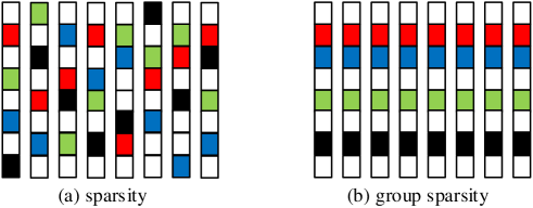
Figure 1: Comparison between sparsity (where columns are sparse, but do not alignment) and group sparsity (where columns are sparse and aligned).

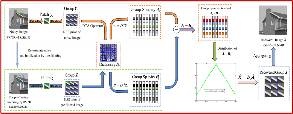
Figure 2: Flowchart of image denoising by group sparsity residual constraint (GSRC) model.

III-B Group Sparsity Residual Constraint

Let us revisit Eq. (1) and Eq. (2), due to the influence of noise, it is very difficult to estimate the true group sparse code B from noisy image Y. In other words, the group sparse code A obtained by solving Eq. (2) is expected to be close enough to the true group sparse code B of the original image X in Eq. (1). As a consequence, the quality of image denoising largely depends on the level of the group sparsity residual, which is defined as the difference between group sparse code A and true group sparse code B,

$${{\textbf{\emph{R}}}}={{\textbf{\emph{A}}}}-{{\textbf{\emph{B}}}}$$ (3)

Therefore, to reduce the group sparsity residual R and boost the accuracy of A, we propose a new prior model to image denoising, called group sparse residual constraint (GSRC) [39], and thus Eq. (2) can be rewritten as

$${{\textbf{\emph{A}}}_{i}}=\arg\min_{{\textbf{\emph{A}}}_{i}}\{||{\textbf{\emph{Y}}}_{i}-{\textbf{\emph{D}}}_{i}{{\textbf{\emph{A}}}_{i}}||_{F}^{2}+\lambda_{i}||{{\textbf{\emph{A}}}_{i}}-{{\textbf{\emph{B}}}_{i}}||_{p}\}$$ (4)

However, it can be seen that the true group sparse code B and $p$ are unknown since the original image X is not available. Therefore, we will discuss how to obtain B and $p$. In addition, one important issue of the proposed GSRC based image denoising is the selection of the dictionary. To adapt to the local image structures, instead of learning an over-complete dictionary for each group ${{\textbf{\emph{Y}}}}_{i}$ as in [10], we learn the principle component analysis (PCA) based dictionary [19] for each group ${{\textbf{\emph{Y}}}}_{i}$.

III-C Estimation of the Unknown Group Sparse Code

Eq. (3) shows that by reducing the group sparsity residual R, we could improve the performance of image denoising. In general, the original image X is not available in practice, and thus the true group sparse code B is unknown. However, the true group sparse code B can be estimated based on prior knowledge of the original image X we have. For example, if we have many example images similar to the original image X, then a good estimation of B could be learned from the example image set. However, under many practical situations, the example image set is simply and unsuitable.

The strategy of pre-filtering is a popular means to image denoising. The basic idea is similar to many denoising algorithms such as BM3D [9] where a first stage pilot denoising is exploited before going to the second stage of the actual denoising. In past few years, a variety of image denoising methods based on pre-filtering have been developed, such as LPG-PCA [40], TID [41], SOS [42], and aGMM [43] methods, etc.

Based on the above analysis, we first apply pre-filtering (e.g., BM3D [9], EPLL [44]) to noisy image Y, and then the initialization result of pre-filtering is defined as Z. Since the pre-filtering has an ideal denoising performance, Z could be regarded as a good approximation of the original image X. Therefore, in this paper the group sparse code B is achieved by the pre-filtering Z. The flowchart of the proposed GSRC is illustrated in Fig. 2. Specifically, to reduce the group sparsity residual, we first obtain a good estimation of the group sparse coefficients of the original image by pre-filtering Z and then the group sparse coefficients of noisy input image are used to approximate this estimate.

III-D Adaptive Patch Search Scheme

$k$ Nearest Neighbors ($k$NN) method [45] has been widely used to nonlocal similar patch selection. Given a noisy reference patch and a target dataset, the aim of $k$NN is to find the $k$ most similar patches. However, since the given reference patch is noisy, $k$NN has a drawback that some of the $k$ selected patches may not be truly similar to given reference patch. For instance, the noisy similar patches via $k$NN and the clean patches matched with these noisy similar patch indexes are shown in Fig. 3(a) and Fig. 3(b), respectively. It can be seen that the 7-th patch (red box) is obviously deviating from given reference patch (green box) in Fig. 3(b). Since the pre-filtered image is regarded as a good estimation of the original image, in this paper we first adopt pre-filtering result as the target image to fetch the $k$ most similar patch indexes. Fig. 3(c) shows the similar patches of BM3D-based pre-filtered image searched by $k$NN and Fig. 3(d) shows the clean patches matched with the pre-filtered image similar patch indexes. It can be seen that the similar patch selection of the pre-filtered image is more accurate than that of the noisy image. Therefore, to obtain an effective similar patch indexes via $k$NN, an adaptive patch search scheme is designed. We define the following formula,

$$\partial={\rm SSIM}({{\textbf{\emph{Z}}}},{\hat{{\textbf{\emph{X}}}}}^{\ell+1})-{\rm SSIM}({{\textbf{\emph{Z}}}},{\hat{{\textbf{\emph{X}}}}}^{\ell})$$ (5)

where SSIM represents structural similarity [46] and ${\hat{{\textbf{\emph{X}}}}}^{\ell}$ represents the $\ell$-th iteration denoising result. We empirically define that if $\partial<\tau$, ${\hat{{\textbf{\emph{X}}}}}^{\ell+1}$ is regarded as target image to fetch the $k$ similar patch indexes, otherwise Z is regarded as target image. Z is the pre-filtered image and $\tau$ is a small constant.

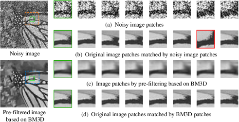
Figure 3: Patch selection between noisy image and pre-filtered image based on BM3D via $k$NN method (where green box represents the reference patch).

III-E Discussion

This subsection will provide detailed discussion about the main difference among the proposed GSRC method, the BM3D mehod[9], the NCSR method [19] and most existing NSS prior-based denoising methods.

• It can be seen that the proposed GSRC method is similar to BM3D method, both of them are two stage-based denoising methods. Nonetheless, the BM3D is based on filtering method (e.g., DST, DCT), while the proposed GSRC is based on sparse coding method, along with dictionary learning. Compared with the analytically designed dictionaries (e.g., DCT/wavelet dictionary), dictionaries learned from image patch/group have an advantage of being better adapted to image local structures [6, 11], and thus could enhance the sparsity which leads to better performance. Moreover, in the second stage of BM3D, they are mixing up the pre-filtered image group with the noisy image group unmannerly, and the Winner filtering is utilized. However, we propose a new prior model, called group sparsity residual constraint (GSRC). Unlike the BM3D method, we do not mix up the pre-filtering image group with the noisy image group, instead, we adopt an iterative shrinkage algorithm [49] to solve the proposed GSRC model, which can better integrate these two NSS priors of noisy and pre-filtered images (Section IV for more details).

• Natural images often possess similar repetitive patterns, i.e., a large number of nonlocal redundancies [8]. By searching many nonlocal patches similar to given reference patch, NCSR [19] first obtained good estimates of the sparse coding coefficients of the original image by the principle of NLM, and then centralized the sparse coding coefficients of the observed image to those estimates to improve the performance of denoising. However, due to the fact that NLM depends on the weighted graph [22], it is unavoidable that the weighted manner leads to disturbance and inaccuracy [23]. It is worth mentioning that the proposed GSRC model does not involve in the weighted graph. In addition, NCSR is actually a patch-based sparse representation method, which usually neglects the relationships among similar patches [24, 72].

• NSS prior has shown great success in image denoising. Most existing denoising methods only exploit the NSS prior of noisy image [10, 19, 25, 26, 59, 27, 47], and few methods use the NSS prior from natural images [48]. Actually, different from the most existing NSS prior-based denoising methods, in this work we consider two kinds of NSS prior, i.e., NSS priors of noisy and pre-filtered images. Experimental results show that the proposed GSRC scheme outperforms many state-of-the-art methods, such as BM3D [9] and WNNM [27] (See Section V for more details).

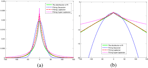
Figure 4: The distribution of the group sparsity residual R for image lena with $\sigma$=30 and fitting Gaussian, Laplacian and hyper-Laplacian distribution in (a) linear and (b) log domain, respectively (pre-filtering based on BM3D [9]).

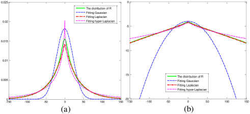
Figure 5: The distribution of the group sparsity residual R for image House with $\sigma$=50 and fitting Gaussian, Laplacian and hyper-Laplacian distribution in (a) linear and (b) log domain, respectively (pre-filtering based on EPLL [44]).

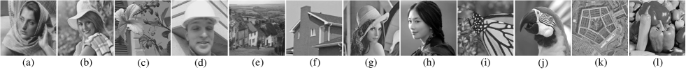
Figure 6: The 12 test images for denoising experiments. (a) Barbara; (b) Elaine; (c) flower; (d) foreman; (e) Hill; (f) House; (g) lena; (h) lin; (i) Monarch; (j) Parrot; (k) pentagon; (l) peppers.

IV Algorithm of GSRC

IV-A Setting of the Parameter $p$

In Eq. (4), except for estimating B, we also need to set the value of $p$. Here we perform some experiments to investigate the statistical property of the group sparsity residual R, where R represents the set of ${{\textbf{\emph{R}}}}_{i}={{\textbf{\emph{A}}}}_{i}-{{\textbf{\emph{B}}}}_{i}$. In these experiments, two images lena and House are used as examples, where Gaussian white noise is added to the images lena and House with standard deviation $\sigma$= 30 (pre-filtering based on BM3D) and $\sigma$= 50 (pre-filtering based on EPLL), respectively. We plot the histogram of R as well as the fitting Gaussian, Laplacian and hyper-Laplacian distribution of R in Fig. 4(a) and Fig. 5(a). To better observe the fitting of the tails, we also plot these distributions in the log domain in Fig. 4(b) and Fig. 5(b). It can be seen that the histogram of R can be well characterized by the Laplacian distribution. Therefore, we set $p=1$ and the $\ell_{1}$-norm is adopted to regularize each group sparsity residual ${{\textbf{\emph{R}}}_{i}}$, and Eq. (4) can be rewritten as

$${{\textbf{\emph{A}}}_{i}} =\arg\min_{{\textbf{\emph{A}}}_{i}}\{||{\textbf{\emph{Y}}}_{i}-{\textbf{\emph{D}}}_{i}{{\textbf{\emph{A}}}_{i}}||_{F}^{2}+\lambda_{i}||{{\textbf{\emph{A}}}_{i}}-{{\textbf{\emph{B}}}_{i}}||_{1}\}$$ (6)

$$=\arg\min_{\tilde{\boldsymbol{\alpha}}_{i}}\{||\tilde{{\textbf{\emph{y}}}}_{i}-\tilde{{\textbf{\emph{D}}}}_{i}{\tilde{\boldsymbol{\alpha}}_{i}}||_{2}^{2}+\lambda_{i}||{\tilde{\boldsymbol{\alpha}}_{i}}-{\tilde{\boldsymbol{\beta}}_{i}}||_{1}\}$$

where $\tilde{{\textbf{\emph{y}}}}_{i},{\tilde{\boldsymbol{\alpha}}_{i}}$, and ${\tilde{\boldsymbol{\beta}}_{i}}$ denote the vectorization of the matrix ${{\textbf{\emph{Y}}}_{i}},{{\textbf{\emph{A}}}_{i}}$ and ${{\textbf{\emph{B}}}_{i}}$, respectively. Each column $\tilde{{\textbf{\emph{d}}}}_{j}$ of the matrix $\tilde{{\textbf{\emph{D}}}}_{i}=[\tilde{{\textbf{\emph{d}}}}_{1},\tilde{{\textbf{\emph{d}}}}_{2},...,\tilde{{\textbf{\emph{d}}}}_{J}]$ denotes the vectorization of the rank-one matrix, where $J$ denotes the number of dictionary atoms.

IV-B Iterative Shrinkage Algorithm to Solve the Proposed GSRC Model

For fixed ${\tilde{\boldsymbol{\beta}}_{i}},\lambda_{i}$, Eq. (6) is convex and can be solved efficiently. We adopt an iterative shrinkage algorithm in [49] to solve Eq. (6). In the $\ell+1$-iteration, the proposed shrinkage operator can be calculated as

$${\tilde{\boldsymbol{\alpha}}_{i}}^{\ell+1}={{{\textbf{\emph{S}}}}_{\lambda_{i}}}({\tilde{{\textbf{\emph{D}}}}_{i}}^{-1}{{\hat{\tilde{{\textbf{\emph{x}}}}}}_{i}}^{\ell}-{{\tilde{\boldsymbol{\beta}}_{i}}})+{{\tilde{\boldsymbol{\beta}}_{i}}}$$ (7)

where ${{{\textbf{\emph{S}}}}_{\lambda_{i}}}(\cdot)$ is the soft-thresholding operator, ${{\hat{\tilde{{\textbf{\emph{x}}}}}}_{i}}$ represents the vectorization of the $i$-th reconstructed group ${{\hat{{\textbf{\emph{X}}}}}_{i}}$. In fact, according to Eq. (7), one can observe that these two NSS priors can be better integrated into this surrogate algorithm. The above shrinkage operator follows the standard surrogate algorithm, from which more details can be seen in [49].

IV-C Adaptive Group Sparsity Regularization Parameter Setting

The parameter $\lambda_{i}$ for each group that balances the fidelity term and the regularization term should be adaptively determined for better denoising performance. In this subsection, inspired by [1], we propose a more robust method for computing $\lambda_{i}$ of Eq. (6) by formulating the group sparse estimation as a Maximum A-Posterior (MAP) estimation problem. For a given ${{\textbf{\emph{B}}}_{i}}$, the optimal solution of Eq. (6) is ${\hat{{{\textbf{\emph{R}}}}}}_{i}=\arg\max\limits_{{\textbf{\emph{R}}}_{\emph{i}}}\rm log\ \emph{P}({{\textbf{\emph{R}}}_{\emph{i}}}|{\textbf{\emph{Y}}}_{\emph{i}})$. By Bayes’ formula, it is equivalent to

$${\hat{{{\textbf{\emph{R}}}}}}_{i} =\arg\max_{{\textbf{\emph{R}}}_{\emph{i}}}\{\rm log\ \emph{P}({{\textbf{\emph{R}}}_{\emph{i}}}|{\textbf{\emph{Y}}}_{\emph{i}})\}$$ (8)

$$=\arg\min\limits_{{\textbf{\emph{R}}}_{\emph{i}}}\{-\rm log\ \emph{P}({\textbf{\emph{Y}}}_{\emph{i}}|{{\textbf{\emph{R}}}_{\emph{i}}})-\rm log\ \emph{P}({{\textbf{\emph{R}}}_{\emph{i}}})\}$$

The log-likelihood term $\rm log\ \emph{P}({{\textbf{\emph{R}}}_{\emph{i}}}|{\textbf{\emph{Y}}}_{\emph{i}})$ is characterized by the statistics of noise V, which is assumed to be additive white Gaussian noise with standard deviation $\sigma$, and thus we have

$$\emph{P}({\textbf{\emph{Y}}}_{\emph{i}}|{{\textbf{\emph{R}}}_{\emph{i}}})=\emph{P}({\textbf{\emph{Y}}}_{\emph{i}}|{{\textbf{\emph{A}}}_{\emph{i}}},{{\textbf{\emph{B}}}_{\emph{i}}}) ={\rm exp}(-\frac{1}{2{\sigma}^{2}}||{\textbf{\emph{Y}}}_{\emph{i}}-{{\textbf{\emph{D}}}_{\emph{i}}}{{\textbf{\emph{A}}}_{\emph{i}}}||_{F}^{2})$$ (9)

where ${{\textbf{\emph{R}}}_{\emph{i}}}$ and ${{\textbf{\emph{B}}}_{\emph{i}}}$ are assumed to be independent. Since the group sparsity residual ${{\textbf{\emph{R}}}_{\emph{i}}}$ can be well characterized by the Laplacian distribution from Fig. 4 and Fig. 5. Thus, the prior distribution $\emph{P}({{\textbf{\emph{R}}}_{\emph{i}}})$ is characterized by an i.i.d Laplacian distribution,

$$\emph{P}({{\textbf{\emph{R}}}_{\emph{i}}})=\frac{c}{\sqrt{2}\sigma_{\emph{i}}}\rm exp(-\frac{\emph{c}\sqrt{2}|{{\textbf{\emph{R}}}_{\emph{i}}}|}{\sigma_{\emph{i}}})$$ (10)

Then we substitute Eq. (9) and Eq. (10) into Eq. (8), and thus we can readily derive the desired regularization parameter $\lambda_{i}$ for each group,

$$\lambda_{i}=\frac{c*2\sqrt{2}{\sigma}^{2}}{\sigma_{i}}$$ (11)

where $\sigma_{i}$ denotes the estimated variance of each group sparsity residual ${\textbf{\emph{R}}}_{i}$, and $c$ is a small constant.

TABLE I: Group sparsity residual constraint for image denoising.

Input:  Noisy image Y.

$\rm\textbf{Initialization:}\ {\hat{{\textbf{\emph{X}}}}}={{\textbf{\emph{Y}}}},{{\textbf{\emph{Z}}}},\emph{c},\emph{k},\emph{b},\emph{L},\sigma,\tau,\gamma,\delta$;

For $\ell=1,2,...,K$ do

Iterative regularization ${{\textbf{\emph{Y}}}}^{\ell+1}={\hat{\textbf{\emph{X}}}}^{\ell}+\delta({{\textbf{\emph{Y}}}}-{\hat{\textbf{\emph{X}}}}^{\ell})$;

Re-estimate $\sigma^{\ell+1}$ computing by Eq. (12);

If   $\ell=1$

Similar patch indexes selection based on Z.

Else

If   ${\rm SSIM}({{\textbf{\emph{Y}}}}^{\ell+1},{{\textbf{\emph{Z}}}})-{\rm SSIM}({{\textbf{\emph{Y}}}}^{\ell},{{\textbf{\emph{Z}}}})<\tau$

Similar patch indexes selection based on ${{\textbf{\emph{Y}}}}^{\ell+1}$.

Else

Similar patch indexes selection based on Z.

End if

End if

For each patch ${{\textbf{\emph{y}}}}_{i}$ and ${{\textbf{\emph{z}}}}_{i}$ do

Find a group ${{{\textbf{\emph{Y}}}}_{i}}^{\ell+1}$ via $k$NN.

Find a group ${{{\textbf{\emph{Z}}}}_{i}}^{\ell+1}$ via $k$NN.

Constructing dictionary ${{{\textbf{\emph{D}}}}_{i}}^{\ell+1}$ by ${{{\textbf{\emph{Y}}}}_{i}}^{\ell+1}$ by PCA operator.

Update ${{{\textbf{\emph{B}}}}_{i}}^{\ell+1}$ computing by ${{\textbf{\emph{B}}}}_{i}={{{\textbf{\emph{D}}}}_{i}}^{-1}{{\textbf{\emph{Z}}}}_{i}$.

Update ${\lambda_{i}}^{t+1}$ computing by Eq. (11).

Update ${{{\textbf{\emph{A}}}}_{i}}^{\ell+1}$ computing by Eq. (7).

Get the estimation ${{{\textbf{\emph{X}}}}_{i}}^{\ell+1}$ =${{{\textbf{\emph{D}}}}_{i}}^{\ell+1}$${{{\textbf{\emph{A}}}}_{i}}^{\ell+1}$.

End for

Aggregate ${{{\textbf{\emph{X}}}}_{i}}^{\ell+1}$ to form the recovered image ${\hat{{\textbf{\emph{X}}}}}^{\ell+1}$.

End for

Output: ${\hat{\textbf{\emph{X}}}}^{\ell+1}$.

With the solution ${{\textbf{\emph{A}}}_{i}}$ in Eq. (7), the clean group ${{\textbf{\emph{X}}}_{i}}$ can be reconstructed as ${{\hat{\textbf{\emph{X}}}}_{i}}={{\textbf{\emph{D}}}_{i}}{{\textbf{\emph{A}}}_{i}}$. Then the latent clean image ${{\hat{\textbf{\emph{X}}}}}$ can be reconstructed by aggregating all the groups $\{{{\textbf{\emph{X}}}_{i}}\}$. In practical, we could perform the above denoising procedures for better results by several iterations. In the $\ell$-th iteration, the iterative regularization strategy [50] is used to update the estimation of noise variance. Then the standard deviation of noise in $\ell$-th iteration is adjusted as

$${\sigma^{\ell}}=\gamma*\sqrt{({\sigma^{2}-||{{\textbf{\emph{Y}}}}-{\hat{{\textbf{\emph{X}}}}}^{\ell}||_{2}^{2}})}$$ (12)

where $\gamma$ is a constant. The complete description of the proposed method for image denoising based on GSRC model is exhibited in Table I.

V Experimental Results

In this section, extensive experimental results are presented to evaluate the denoising performance of the proposed GSRC. For the test images, we use two different test datasets for thorough evaluation. One is a test dataset containing 200 natural images from Berkeley segmentation dataset (BSD200) [51] and the other one contains 12 images which are shown in Fig. 6. We consider two versions of pre-filtering: (1) a pre-filtered image Z generated by the BM3D method [9], denoted as GSRC-BM3D; (2) a pre-filtered image Z generated by the EPLL method [44], denoted as GSRC-EPLL. To evaluate the quality of denoised image, both PSNR and SSIM [46] metrics are used.

V-A Parameter Setting

Parameters used in the algorithm are empirically chosen in consideration of the noise levels in order to achieve relatively good performance. The basic parameter setting is as follows: the searching window $L\times L$ is set to be $30\times 30$. The size of patch $\sqrt{b}\times\sqrt{b}$ is set to be $6\times 6$, $7\times 7$, $8\times 8$ and $9\times 9$ for $\sigma\leq 20$, $20<\sigma\leq 50$, $50<\sigma\leq 75$ and $75<\sigma\leq 100$, respectively. The searching matched patches $k$ is set to be 60, 80, 90 for $\sigma\leq 50$, $50<\sigma\leq 75$ and $75<\sigma\leq 100$, respectively. The detailed setting of the involved parameters $c$, $\delta$, $\gamma$ and $\tau$ are shown in Table II. We run denoising experiments for a large range of noise standard deviations ($\sigma$= 20, 30, 40, 50, 75 and 100).

TABLE II: The detailed involved parameters setting of $c,\delta,\gamma,\tau$.

Noise level	GSRC-BM3D				GSRC-EPLL
$\sigma$	c	$\delta$	$\gamma$	$\tau$	c	$\delta$	$\gamma$	$\tau$
$\sigma\leq 20$	0.2	0.2	0.7	1e-4	0.3	0.1	0.5	5e-4
$20<\sigma\leq 30$	0.4	0.1	0.5	7e-4	0.3	0.1	0.5	5e-4
$30<\sigma\leq 40$	0.2	0.2	0.7	6e-5	0.3	0.1	0.5	6e-4
$40<\sigma\leq 50$	0.5	0.1	0.4	6e-5	0.5	0.1	0.4	4e-4
$50<\sigma\leq 75$	0.9	0.1	0.3	6e-5	0.9	0.1	0.3	1e-4
$75<\sigma\leq 100$	1	0.1	0.3	2e-4	0.9	0.1	0.3	2e-4

TABLE III: PSNR (dB) values of denoising results for four competing state-of-the-art image denosing methods. Top Left: BM3D [9]; Top Right: EPLL [44]; Bottom Left: GSRC-BM3D; Bottom Right: GSRC-EPLL.

$\sigma$	20		30		40		50		75		100
Barbara	31.24	29.85	29.08	27.58	27.26	25.99	26.42	24.86	24.53	23.00	23.20	21.89
	31.65	31.56	29.50	29.42	27.92	27.85	26.80	26.54	24.80	24.52	23.57	23.42
Elaine	32.51	32.16	30.52	30.15	28.95	28.73	27.96	27.63	25.93	25.60	24.48	24.16
	32.63	32.65	30.61	30.66	29.09	29.14	28.07	28.02	26.14	26.11	24.74	24.67
flower	30.01	30.01	27.97	27.95	26.48	26.55	25.49	25.51	23.82	23.59	22.66	22.39
	30.47	30.41	28.28	28.32	26.92	26.93	25.92	25.89	24.17	24.16	22.94	22.89
foreman	34.54	33.67	32.75	31.70	31.29	30.28	30.36	29.20	28.07	27.24	26.51	25.91
	34.81	34.82	33.34	33.34	32.00	32.13	31.06	31.04	29.12	29.12	27.75	27.77
Hill	30.20	30.12	28.41	28.28	27.11	27.04	26.28	26.10	24.71	24.50	23.62	23.47
	30.29	30.28	28.45	28.47	27.24	27.23	26.35	26.29	24.82	24.78	23.82	23.78
House	33.77	32.99	32.09	31.24	30.65	29.89	29.69	28.79	27.51	26.70	25.87	25.21
	34.08	34.03	32.63	32.54	31.47	31.45	30.43	30.45	28.48	28.53	26.95	26.97
lena	31.52	31.25	29.46	29.18	27.82	27.78	26.90	26.68	25.17	24.75	23.87	23.46
	31.87	31.83	29.76	29.78	28.31	28.30	27.31	27.22	25.56	25.52	24.39	24.41
lin	32.83	32.62	30.95	30.67	29.52	29.32	28.71	28.26	26.96	26.36	26.00	25.05
	33.06	33.03	31.18	31.13	29.85	29.86	28.93	28.90	27.19	27.17	25.99	25.97
Monarch	30.35	30.49	28.36	28.36	26.72	26.89	25.82	25.78	23.91	23.73	22.52	22.24
	31.07	31.10	28.83	28.88	27.43	27.45	26.38	26.41	24.43	24.49	23.06	23.09
Parrot	32.32	32.00	30.33	30.00	28.64	28.60	27.88	27.53	25.94	25.56	24.60	24.08
	32.64	32.58	30.75	30.68	29.38	29.33	28.35	28.29	26.33	26.31	24.94	24.96
pentagon	28.23	27.96	26.41	26.06	25.10	24.79	24.21	23.83	22.59	22.18	21.45	21.12
	28.61	28.57	26.63	26.60	25.35	25.30	24.42	24.39	22.89	22.83	21.81	21.73
peppers	30.49	30.46	28.66	28.66	27.26	27.35	26.17	26.35	24.43	24.49	23.17	23.25
	30.72	30.72	28.81	28.84	27.51	27.56	26.53	26.56	24.67	24.70	23.44	23.46
Average	31.50	31.13	29.58	29.15	28.07	27.77	27.16	26.71	25.30	24.81	23.96	23.52
	31.83	31.80	29.90	29.89	28.54	28.54	27.55	27.50	25.72	25.69	24.45	24.43

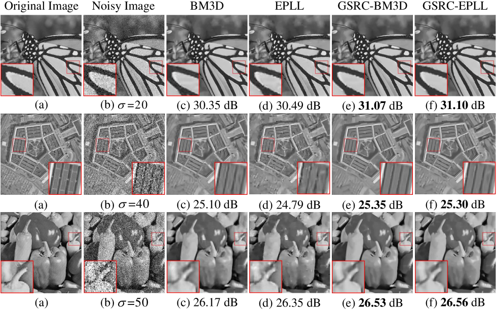
Figure 7: Denoising results of BM3D, EPLL, GSRC-BM3D and GSRC-EPLL on test image $\emph{Monarch},\emph{pentagon}$ and peppers with $\sigma=20,40$ and 50, respectively. (a) Original image; (b) Noisy Image; (c) Pre-filtering BM3D [9] results. (d) Pre-filtering EPLL [44] results; (e) GSRC-BM3D results; (f) GSRC-EPLL results.

TABLE IV: PSNR (dB) Comparison of NCSR [19], GID [52], LINC [53], MS-EPLL [54], AST-NLS [55], WNNM [27], GSRC-BM3D and GSRC-EPLL.

	$\sigma=20$								$\sigma=30$
	NCSR	GID	LINC	MS-	AST-	WNNM	GSRC-	GSRC-	NCSR	GID	LINC	MS-	AST-	WNNM	GSRC-	GSRC-
				EPLL	NLS		BM3D	EPLL				EPLL	NLS		BM3D	EPLL
Barbara	31.10	29.81	31.70	30.07	31.43	31.60	31.65	31.56	28.68	27.35	29.53	27.72	29.13	29.68	29.50	29.42
Elaine	32.39	31.23	32.59	32.50	32.45	32.55	32.63	32.65	30.25	28.98	30.39	30.53	30.32	30.75	30.61	30.66
flower	30.05	29.12	30.30	30.10	30.28	30.34	30.47	30.41	27.86	27.01	28.13	28.05	28.20	28.26	28.29	28.32
foreman	34.42	33.08	34.76	34.09	34.55	34.73	34.81	34.82	32.61	30.92	32.93	32.34	32.79	33.00	33.34	33.34
Hill	30.03	29.06	30.14	30.20	30.22	30.27	30.29	30.29	28.15	27.05	28.29	28.41	28.37	28.41	28.45	28.47
House	33.81	32.68	33.82	33.27	33.87	34.01	34.08	34.03	32.01	30.50	32.26	31.71	32.26	32.52	32.63	32.54
lena	31.48	30.33	31.80	31.48	31.63	31.72	31.87	31.83	29.32	28.36	29.82	29.46	29.50	29.45	29.76	29.78
lin	32.66	31.74	33.04	32.80	32.84	33.00	33.06	33.03	30.65	29.63	31.03	30.96	30.83	31.07	31.18	31.13
Monarch	30.52	29.75	30.64	30.59	30.84	31.10	31.07	31.11	28.38	27.68	28.74	28.49	28.70	28.91	28.83	28.88
Parrot	32.25	31.24	32.50	32.21	32.42	32.66	32.64	32.58	30.20	29.33	30.64	30.29	30.37	30.78	30.75	30.68
pentagon	28.27	27.39	28.43	27.99	28.49	28.49	28.61	28.57	26.27	25.32	26.42	26.05	26.57	26.67	26.63	26.60
peppers	30.35	29.78	30.50	30.60	30.61	30.70	30.72	30.72	28.41	27.86	28.79	28.85	28.75	28.84	28.81	28.84
Average	31.45	30.43	31.69	31.32	31.64	31.76	31.83	31.80	29.40	28.33	29.75	29.41	29.65	29.86	29.90	29.89
	$\sigma=40$								$\sigma=50$
	NCSR	GID	LINC	MS-	AST-	WNNM	GSRC-	GSRC-	NCSR	GID	LINC	MS-	AST-	WNNM	GSRC-	GSRC-
				EPLL	NLS		BM3D	EPLL				EPLL	NLS		BM3D	EPLL
Barbara	27.25	25.77	27.77	26.05	27.41	27.86	27.92	27.85	26.13	24.52	26.27	25.06	26.43	26.83	26.80	26.54
Elaine	28.91	27.67	28.96	29.13	28.69	29.05	29.09	29.14	27.68	26.54	27.73	27.98	27.68	28.08	28.07	28.02
flower	26.35	25.60	26.79	26.64	26.75	26.85	26.92	26.93	25.31	24.42	25.47	25.56	25.77	25.80	25.92	25.89
foreman	31.52	29.61	31.31	31.05	31.29	31.54	32.00	32.13	30.41	28.64	30.33	30.04	30.46	30.75	31.06	31.04
Hill	26.91	25.87	26.84	27.18	27.05	27.29	27.24	27.23	26.01	25.05	26.03	26.28	26.16	26.14	26.35	26.29
House	30.79	29.02	31.00	30.47	30.91	31.31	31.47	31.46	29.61	27.76	29.87	29.47	30.13	30.32	30.43	30.45
lena	28.00	26.98	28.13	28.05	28.00	28.43	28.31	28.30	26.94	25.82	26.94	26.97	27.08	27.26	27.31	27.22
lin	29.27	28.44	29.94	29.68	29.39	29.78	29.85	29.86	28.23	27.50	28.85	28.69	28.50	28.83	28.93	28.90
Monarch	26.81	26.32	27.14	27.06	27.20	27.47	27.43	27.45	25.73	25.28	25.88	25.93	26.12	26.18	26.38	26.41
Parrot	28.77	28.01	29.26	28.94	28.87	29.33	29.38	29.33	27.67	26.79	28.23	27.90	27.92	28.15	28.35	28.29
pentagon	24.93	23.95	24.96	24.75	25.22	25.41	25.35	25.30	23.94	22.81	23.85	23.81	24.31	24.46	24.42	24.39
peppers	27.09	26.47	27.39	27.57	27.37	27.70	27.51	27.56	26.02	25.48	26.47	26.55	26.36	26.56	26.53	26.56
Average	28.05	26.97	28.29	28.05	28.18	28.50	28.54	28.55	26.97	25.88	27.16	27.02	27.24	27.44	27.55	27.50
	$\sigma=75$								$\sigma=100$
	NCSR	GID	LINC	MS-	AST-	WNNM	GSRC-	GSRC-	NCSR	GID	LINC	MS-	AST-	WNNM	GSRC-	GSRC-
				EPLL	NLS		BM3D	EPLL				EPLL	NLS		BM3D	EPLL
Barbara	24.06	22.43	24.04	23.19	24.40	24.79	24.80	24.52	22.70	21.40	22.39	22.11	23.19	23.26	23.57	23.42
Elaine	25.34	24.54	25.42	25.99	25.51	25.94	26.14	26.11	23.77	23.21	23.92	24.52	23.94	24.54	24.74	24.67
flower	23.50	22.72	23.30	23.68	23.87	23.88	24.17	24.16	22.22	20.69	21.96	22.50	22.50	22.70	22.94	22.89
foreman	28.18	26.71	28.11	28.14	28.54	28.48	29.12	29.12	26.55	25.33	26.55	26.84	27.32	27.39	27.75	27.77
Hill	24.43	23.62	24.13	24.72	24.42	24.70	24.82	24.79	23.27	22.75	23.21	23.74	23.33	23.63	23.82	23.78
House	27.16	25.23	27.56	27.45	28.06	28.25	28.48	28.53	25.49	22.38	26.11	25.99	26.52	26.68	26.95	26.97
lena	25.02	23.78	25.12	25.11	25.32	25.38	25.56	25.52	23.63	22.43	23.67	23.91	24.17	24.08	24.39	24.41
lin	26.22	25.50	26.86	26.91	26.72	26.94	27.19	27.17	24.85	24.14	25.23	25.63	25.42	25.67	25.99	25.97
Monarch	23.67	22.77	23.91	23.92	24.11	24.31	24.43	24.49	22.10	20.73	22.13	22.44	22.68	22.95	23.06	23.09
Parrot	25.45	24.87	26.20	25.92	25.93	26.32	26.33	26.31	23.94	23.54	24.48	24.38	24.61	24.85	24.94	24.96
pentagon	22.04	21.31	22.26	22.19	22.49	22.65	22.89	22.83	20.92	19.53	21.05	21.15	21.24	21.56	21.81	21.73
peppers	24.07	23.44	24.44	24.74	24.47	24.61	24.67	24.70	22.68	22.09	22.83	23.51	23.18	23.19	23.44	23.46
Average	24.93	23.91	25.11	25.16	25.32	25.52	25.72	25.69	23.51	22.35	23.63	23.89	24.01	24.21	24.45	24.43

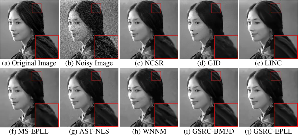
Figure 8: Denoising images of lin by different methods ($\sigma=30$). (a) Original image; (b) Noisy image; (c) NCSR [19] (PSNR= 30.65dB, SSIM=0.8632); (d) GID [52] (PSNR= 29.63dB, SSIM=0.8287); (e) LINC [53] (PSNR= 31.03dB, SSIM=0.8670); (f) MS-EPLL [54] (PSNR= 30.96dB, SSIM=0.8688); (g) AST-NLS [55] (PSNR= 30.83dB, SSIM=0.8465); (h) WNNM [27] (PSNR= 31.07dB, SSIM=0.8657); (i) GSRC-BM3D (PSNR= 31.18dB, SSIM =0.8743); (j) GSRC-EPLL (PSNR = 31.13dB, SSIM=0.8704).

V-B Performance Comparison with the State-of-the-Art Methods

In this subsection, we validate the performance of the proposed GSRC and compare it with recently proposed state-of-the-art denoising methods, including BM3D [9], EPLL [44], NCSR [19], GID [52], LINC [53], MS-EPLL [54], AST-NLS [55] and WNNM [27]. For all the competing methods, the source codes are obtained from the original authors. We used the default parameters in their software packages.

First, we compare GSRC-BM3D, GSRC-EPLL with BM3D and EPLL method, respectively. In Table III, we report the PSNR results for different noise variances for the 12 test images in Fig. 6. It can be seen that GSRC-BM3D, GSRC-EPLL are significantly better than BM3D and EPLL with an average gain of about 0.40dB and 0.79dB, respectively. The visual quality comparisons in the case of $\sigma=20,40$ and 50 for test images Monarch, pentagon and peppers are provided in Fig. 7, respectively. It can be found out that the over-smooth phenomena and undesirable artifacts are generated by BM3D and EPLL methods, respectively. In contrast, the proposed GSRC not only reduces most of the artifacts, but also provides better denoising performance on both edges and textures than BM3D and EPLL methods. Therefore, these results validate the usefulness of the proposed GSRC model through the pre-filtering BM3D and EPLL.

Second, to further verify the performance of the proposed GSRC in image denoising, we compare it with six representative algorithms: NCSR [19], GID [52], LINC [53], MS-EPLL [54], AST-NLS [55] and WNNM [27]. Gaussian white noise with standard deviation $\sigma$=20, 30, 40, 50, 75 and 100 is added to the 12 test images. The PSNR results by the competing denoising methods are shown in Table IV. It can be seen that the proposed GSRC has achieved highly competitive denoising performance to other leading methods. Based on the pre-filtering BM3D [9], the proposed GSRC achieves 0.61dB, 1.68dB, 0.39dB, 0.52dB, 0.32dB and 0.11dB improvement on average over NCSR, GID, LINC, MS-EPLL, AST-NLS and WNNM, respectively. Meanwhile, based on the pre-filtering EPLL [44], the proposed GSRC achieves 0.59dB, 1.66dB, 0.37dB, 0.50dB, 0.30dB and 0.09dB improvement on average over NCSR, GID, LINC, MS-EPLL, AST-NLS and WNNM, respectively. The visual comparisons of the competing methods at noise level 30 and 75 are shown in Fig. 8 and Fig. 9, respectively.

TABLE V: Average PSNR (dB) results of different denoising algorithms for Gaussian denoising with noise level 20, 30, 40, 50, 75 and 100 on BSD200 dataset [51].

$\sigma$	20	30	40	50	75	100
NCSR [19]	29.89	27.92	26.58	25.65	24.04	23.00
GID [52]	28.87	27.00	25.87	24.97	23.37	22.20
LINC [53]	29.92	27.94	26.61	25.64	23.98	22.91
MS-EPLL [54]	29.95	28.02	26.73	25.84	24.29	23.27
AST-NLS [55]	29.98	28.02	26.68	25.80	24.20	23.17
WNNM [27]	30.11	28.17	26.88	25.96	24.42	23.37
GSRC-BM3D	30.12	28.15	26.89	26.01	24.49	23.49
GSRC-EPLL	30.11	28.17	26.91	26.00	24.48	23.49

TABLE VI: Average PSNR (dB) results of APS and No-APS scheme on 12 test images.

Pre-filtering	BM3D
$\sigma$	20	30	40	50	75	100
No-APS	31.71	29.74	28.38	27.37	25.56	24.25
APS	31.83	29.90	28.54	27.55	25.72	24.45
Pre-filtering	EPLL
$\sigma$	20	30	40	50	75	100
No-APS	31.71	29.80	28.42	27.36	25.55	24.26
APS	31.80	29.89	28.55	27.50	25.69	24.43

To further demonstrate our performance, we comprehensively evaluate the proposed GSRC on 200 test images from the BSD dataset [51]. Table V lists the average PSNR comparison results for a collection of 200 test images among eight competing methods at six noise levels ($\sigma$=20, 30, 40, 50, 75 and 100). The visual comparisons of the denoising methods for test images 130066 and 223004 with $\sigma=50$ and 100 are shown in Fig. 10 and Fig. 11, respectively. Obviously, one can observe that the proposed GSRC achieves very competitive denoising performance compared to WNNM.

In addition, we apply the proposed GSRC to some real noisy images. Fig. 12 shows the denoised images yielded by BM3D and our approach. It can be seen that the proposed GSRC can not only reduce the noise effectively, but also preserve the finer details. The results indicate the feasibility of the proposed GSRC for some practical image denoising tasks.

TABLE VII: Average run time (s) on the 12 test images (size: $256\times 256$) with different methods.

Methods	NCSR [19]	GID [52]	LINC [53]	MS-EPLL [54]	AST-NLS [55]	WNNM [27]	GSRC-BM3D	GSRC-EPLL
Average Time (s)	348	346	257	191	459	202	72	148

To sum up, it can be easily found that BM3D, EPLL, NCSR, GID, LINC, MS-EPLL, AST-NLS and WNNM still generate some undesirable artifacts and some details are lost. By contrast, the proposed GSRC is able to preserve the sharp edges and suppress undesirable artifacts more effectively than other competing methods. Such experimental findings clearly demonstrate that the GSRC model is a stronger prior for the class of photographic images containing large variations in edges/textures.

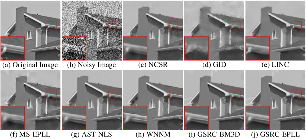
Figure 9: Denoising images of House by different methods ($\sigma=75$). (a) Original image; (b) Noisy image; (c) NCSR [19] (PSNR= 27.16dB, SSIM =0.7749); (d) GID [52] (PSNR= 25.23dB, SSIM=0.7052); (e) LINC [53] (PSNR= 27.56dB, SSIM=0.7850); (f) MS-EPLL [54] (PSNR= 27.45dB, SSIM=0.7738); (g) AST-NLS [55] (PSNR= 28.06dB, SSIM=0.7720); (h) WNNM [27] (PSNR= 28.25dB, SSIM=0.7883); (i) GSRC-BM3D (PSNR= 28.48dB, SSIM=0.7992); (j) GSRC-EPLL (PSNR = 28.53dB, SSIM=0.7998).

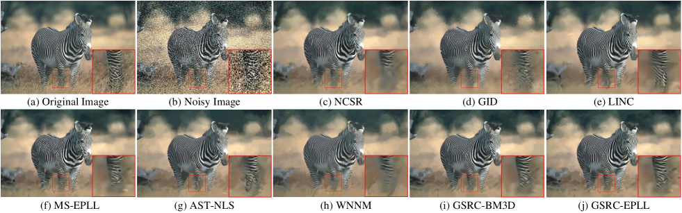
Figure 10: Denoising images of 130066 by different methods ($\sigma=50$). (a) Original image; (b) Noisy image; (c) NCSR [19] (PSNR= 25.69dB, SSIM=0.7800); (d) GID [52] (PSNR= 25.40dB, SSIM=0.7152); (e) LINC [53] (PSNR= 26.51dB, SSIM=0.7938); (f) MS-EPLL [54] (PSNR= 25.67dB, SSIM=0.7833); (g) AST-NLS [55] (PSNR= 26.27dB, SSIM=0.7715); (h) WNNM [27] (PSNR= 26.43dB, SSIM=0.7888); (i) GSRC-BM3D (PSNR= 26.69dB, SSIM=0.7937); (j) GSRC-EPLL (PSNR = 26.62dB, SSIM=0.7908).

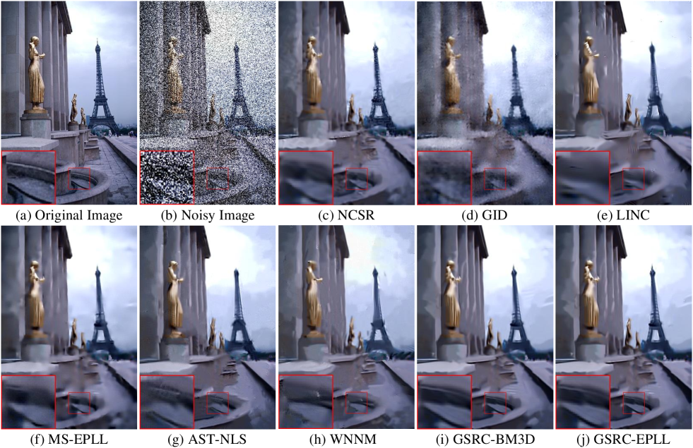
Figure 11: Denoising images of 223004 by different methods ($\sigma=100$). (a) Original image; (b) Noisy image; (c) NCSR [19] (PSNR= 23.73dB, SSIM=0.6882); (d) GID [52] (PSNR= 22.66dB, SSIM=0.5997); (e) LINC [53] (PSNR= 23.68dB, SSIM=0.6756); (f) MS-EPLL [54] (PSNR= 24.21dB, SSIM=0.6869); (g) AST-NLS [55] (PSNR= 24.24dB, SSIM=0.6861); (h) WNNM [27] (PSNR= 24.48dB, SSIM=0.7025); (i) GSRC-BM3D (PSNR= 24.70dB, SSIM =0.7182); (j) GSRC-EPLL (PSNR = 24.67dB, SSIM=0.7157).

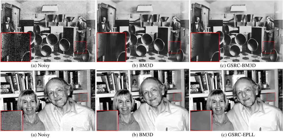
Figure 12: Visual comparisons of denoising results on real noisy images with unknown noise characteristics.

V-C Comparison between APS and No-APS Scheme

In this subsection, in order to demonstrate the designed adaptive patch selection (APS) scheme effectively, we compare it with No-APS scheme. Table VI shows the average PSNR results of APS and No-APS schemes on 12 test images. It can be seen that the average PSNR results of APS scheme are better than No-APS. Therefore, the proposed APS scheme can boost the accuracy of nonlocal similar patch selection under the task of image denoising.

V-D Computational Cost

Efficiency is another key factor in evaluating an algorithm. We then compare the speed of the proposed GSRC and six representative algorithms. All experiments are conducted under the Matlab 2012b environment on a machine with Intel (R) Core (TM) i3-4150 with 3.56Hz CPU and 4GB memory. The average run time (s) of the competing methods on the 12 test images (size: 256$\times$256) is shown in Table VII. Denoising 12 test images, NCSR, GID, LINC, MS-EPLL, AST-NLS and WNNM take, on average, roughly 348s, 346s, 257s, 191s, 459s and 202s, respectively. For the test images, the proposed GSRC requires only 72s and 148s on average based pre-filtering BM3D and EPLL, respectively. Obviously, it can be seen that that the proposed GSRC used less computation time than these representative methods. Note that the run time of the proposed GSRC includes the pre-filtering process.

VI Conclusion

In this paper, we proposed a novel prior model named group sparsity residual constraint (GSRC) that exploited two kinds of nonlocal self-similar (NSS) prior and explored its application into image denoising. To boost the performance of group sparse-based image denoising, the group sparsity residual was proposed, which is defined as the difference between the group sparse code of noisy image and the group sparse code of the original image. Therefore, the problem of image denoising was translated into one that reduces the group sparsity residual. Since the original image was unknown, to reduce the group sparsity residual, we first obtained some good estimation of the group sparse coefficients of the original image by pre-filtering and then the group sparse coefficients of the noisy image were used to approximate the estimation. To enhance the accuracy of nonlocal similar patches selection, an adaptive patch search scheme was designed. In addition, to fuse these two NSS priors better, an iterative shrinkage algorithm was adopted to solve the GSRC model. Extensive experimental results have shown that the proposed GSRC can not only leads to visible PSNR improvements over many state-of-the-art methods such as BM3D and WNNM, but also preserves the image local structures, suppresses undesirable artifacts and results in a competitive speed. In the future, we will extend the proposed GSRC to other applications such as image deblurring, image super-resolution and image deblocking.

References

- [1] Chang S G, Yu B, Vetterli M. Adaptive wavelet thresholding for image denoising and compression[J]. IEEE transactions on image processing, 2000, 9(9): 1532-1546.
- [2] Starck J L, Cand s E J, Donoho D L. The curvelet transform for image denoising[J]. IEEE Transactions on image processing, 2002, 11(6): 670-684.
- [3] Remenyi N, Nicolis O, Nason G, et al. Image denoising with 2D scale-mixing complex wavelet transforms[J]. IEEE Transactions on Image Processing, 2014, 23(12): 5165-5174.
- [4] Rudin L I, Osher S, Fatemi E. Nonlinear total variation based noise removal algorithms[J]. Physica D: Nonlinear Phenomena, 1992, 60(1-4): 259-268.
- [5] Chambolle A. An algorithm for total variation minimization and applications[J]. Journal of Mathematical imaging and vision, 2004, 20(1): 89-97.
- [6] Elad M, Aharon M. Image denoising via sparse and redundant representations over learned dictionaries[J]. IEEE Transactions on Image processing, 2006, 15(12): 3736-3745.
- [7] Protter M, Elad M. Image sequence denoising via sparse and redundant representations[J]. IEEE Transactions on Image Processing, 2009, 18(1): 27-35.
- [8] Buades A, Coll B, Morel J M. A non-local algorithm for image denoising[C]//Computer Vision and Pattern Recognition, 2005. CVPR 2005. IEEE Computer Society Conference on. IEEE, 2005, 2: 60-65.
- [9] Dabov K, Foi A, Katkovnik V, et al. Image denoising by sparse 3-D transform-domain collaborative filtering[J]. IEEE Transactions on image processing, 2007, 16(8): 2080-2095.
- [10] Mairal J, Bach F, Ponce J, et al. Non-local sparse models for image restoration[C]//Computer Vision, 2009 IEEE 12th International Conference on. IEEE, 2009: 2272-2279.
- [11] Aharon M, Elad M, Bruckstein A. -SVD: An algorithm for designing overcomplete dictionaries for sparse representation[J]. IEEE Transactions on signal processing, 2006, 54(11): 4311-4322.
- [12] Mairal J, Bach F, Ponce J, et al. Online dictionary learning for sparse coding[C]//Proceedings of the 26th annual international conference on machine learning. ACM, 2009: 689-696.
- [13] Mairal J, Bach F, Ponce J. Task-driven dictionary learning[J]. IEEE transactions on pattern analysis and machine intelligence, 2012, 34(4): 791-804.
- [14] Zhang Q, Li B. Discriminative K-SVD for dictionary learning in face recognition[C]//Computer Vision and Pattern Recognition (CVPR), 2010 IEEE Conference on. IEEE, 2010: 2691-2698.
- [15] Mairal J, Elad M, Sapiro G. Sparse representation for color image restoration[J]. IEEE Transactions on image processing, 2008, 17(1): 53-69.
- [16] Jiang Z, Lin Z, Davis L S. Label consistent K-SVD: Learning a discriminative dictionary for recognition[J]. IEEE Transactions on Pattern Analysis and Machine Intelligence, 2013, 35(11): 2651-2664.
- [17] Dong W, Zhang L, Shi G, et al. Image deblurring and super-resolution by adaptive sparse domain selection and adaptive regularization[J]. IEEE Transactions on Image Processing, 2011, 20(7): 1838-1857.
- [18] Jung M, Bresson X, Chan T F, et al. Nonlocal Mumford-Shah regularizers for color image restoration[J]. IEEE transactions on image processing, 2011, 20(6): 1583-1598.
- [19] Dong W, Zhang L, Shi G, et al. Nonlocally centralized sparse representation for image restoration[J]. IEEE Transactions on Image Processing, 2013, 22(4): 1620-1630.
- [20] Zha Z, Liu X, Zhang X, et al. Compressed sensing image reconstruction via adaptive sparse nonlocal regularization[J]. The Visual Computer, 2016: 1-21.
- [21] Elmoataz A, Lezoray O, Bougleux S. Nonlocal discrete regularization on weighted graphs: a framework for image and manifold processing[J]. IEEE transactions on Image Processing, 2008, 17(7): 1047-1060.
- [22] Peyr G. Image processing with nonlocal spectral bases[J]. Multiscale Modeling & Simulation, 2008, 7(2): 703-730.
- [23] Zhang X, Burger M, Bresson X, et al. Bregmanized nonlocal regularization for deconvolution and sparse reconstruction[J]. SIAM Journal on Imaging Sciences, 2010, 3(3): 253-276.
- [24] Zhang J, Zhao D, Gao W. Group-based sparse representation for image restoration[J]. IEEE Transactions on Image Processing, 2014, 23(8): 3336-3351.
- [25] Dong W, Shi G, Ma Y, et al. Image restoration via simultaneous sparse coding: Where structured sparsity meets gaussian scale mixture[J]. International Journal of Computer Vision, 2015, 114(2-3): 217-232.
- [26] Ji H, Liu C, Shen Z, et al. Robust video denoising using low rank matrix completion[C]//Computer Vision and Pattern Recognition (CVPR), 2010 IEEE Conference on. IEEE, 2010: 1791-1798.
- [27] Gu S, Xie Q, Meng D, et al. Weighted nuclear norm minimization and its applications to low level vision[J]. International journal of computer vision, 2017, 121(2): 183-208.
- [28] Engl H W, Kunisch K, Neubauer A. Convergence rates for Tikhonov regularisation of non-linear ill-posed problems[J]. Inverse problems, 1989, 5(4): 523.
- [29] Simoncelli E P, Adelson E H. Noise removal via Bayesian wavelet coring[C]//Image Processing, 1996. Proceedings., International Conference on. IEEE, 1996, 1: 379-382.
- [30] Do M N, Vetterli M. The contourlet transform: an efficient directional multiresolution image representation[J]. IEEE Transactions on image processing, 2005, 14(12): 2091-2106.
- [31] Donoho D L. De-noising by soft-thresholding[J]. IEEE transactions on information theory, 1995, 41(3): 613-627.
- [32] Jain V, Seung S. Natural image denoising with convolutional networks[C]//Advances in Neural Information Processing Systems. 2009: 769-776.
- [33] Li S Z. Markov random field modeling in image analysis[M]. Springer Science & Business Media, 2009.
- [34] Burger H C, Schuler C J, Harmeling S. Image denoising: Can plain neural networks compete with BM3D?[C]//Computer Vision and Pattern Recognition (CVPR), 2012 IEEE Conference on. IEEE, 2012: 2392-2399.
- [35] Shao L, Yan R, Li X, et al. From heuristic optimization to dictionary learning: A review and comprehensive comparison of image denoising algorithms[J]. IEEE Transactions on Cybernetics, 2014, 44(7): 1001-1013.
- [36] Liu L, Chen L, Chen C L P, et al. Weighted joint sparse representation for removing mixed noise in image[J]. IEEE transactions on cybernetics, 2017, 47(3): 600-611.
- [37] Zhang K, Zuo W, Chen Y, et al. Beyond a gaussian denoiser: Residual learning of deep cnn for image denoising[J]. IEEE Transactions on Image Processing, 2017.
- [38] Liu S, Pan J, Yang M H. Learning recursive filters for low-level vision via a hybrid neural network[C]//European Conference on Computer Vision. Springer International Publishing, 2016: 560-576.
- [39] Zha Z, Liu X, Zhou Z, et al. Image denoising via group sparsity residual constraint[C]//Acoustics, Speech and Signal Processing (ICASSP), 2017 IEEE International Conference on. IEEE, 2017: 1787-1791.
- [40] Zhang L, Dong W, Zhang D, et al. Two-stage image denoising by principal component analysis with local pixel grouping[J]. Pattern Recognition, 2010, 43(4): 1531-1549.
- [41] Luo E, Chan S H, Nguyen T Q. Adaptive image denoising by targeted databases[J]. IEEE Transactions on Image Processing, 2015, 24(7): 2167-2181.
- [42] Romano Y, Elad M. Boosting of image denoising algorithms[J]. SIAM Journal on Imaging Sciences, 2015, 8(2): 1187-1219.
- [43] Luo E, Chan S H, Nguyen T Q. Adaptive Image Denoising by Mixture Adaptation[J]. IEEE Transactions on Image Processing, 2016, 25(10): 4489-4503.
- [44] Zoran D, Weiss Y. From learning models of natural image patches to whole image restoration[C]//Computer Vision (ICCV), 2011 IEEE International Conference on. IEEE, 2011: 479-486.
- [45] Larose D T. K-nearest neighbor algorithm[J]. Discovering Knowledge in Data: An Introduction to Data Mining, 2005: 90-106.
- [46] Wang Z, Bovik A C, Sheikh H R, et al. Image quality assessment: from error visibility to structural similarity[J]. IEEE transactions on image processing, 2004, 13(4): 600-612.
- [47] Zhang J, Zhao D, Xiong R, et al. Image restoration using joint statistical modeling in a space-transform domain[J]. IEEE Transactions on Circuits and Systems for Video Technology, 2014, 24(6): 915-928.
- [48] Xu J, Zhang L, Zuo W, et al. Patch group based nonlocal self-similarity prior learning for image denoising[C]//Proceedings of the IEEE international conference on computer vision. 2015: 244-252.
- [49] Daubechies I, Defrise M, De Mol C. An iterative thresholding algorithm for linear inverse problems with a sparsity constraint[J]. Communications on pure and applied mathematics, 2004, 57(11): 1413-1457.
- [50] Osher S, Burger M, Goldfarb D, et al. An iterative regularization method for total variation-based image restoration[J]. Multiscale Modeling & Simulation, 2005, 4(2): 460-489.
- [51] Arbelaez P, Maire M, Fowlkes C, et al. Contour detection and hierarchical image segmentation[J]. IEEE transactions on pattern analysis and machine intelligence, 2011, 33(5): 898-916.
- [52] Talebi H, Milanfar P. Global image denoising[J]. IEEE Transactions on Image Processing, 2014, 23(2): 755-768.
- [53] Niknejad M, Rabbani H, Babaie-Zadeh M. Image restoration using Gaussian mixture models with spatially constrained patch clustering[J]. IEEE Transactions on Image Processing, 2015, 24(11): 3624-3636.
- [54] Papyan V, Elad M. Multi-scale patch-based image restoration[J]. IEEE Transactions on image processing, 2016, 25(1): 249-261.
- [55] Liu H, Xiong R, Zhang J, et al. Image denoising via adaptive soft-thresholding based on non-local samples[C]//Proceedings of the IEEE Conference on Computer Vision and Pattern Recognition. 2015: 484-492.
- [56] Zha Z, Liu X, Huang X, et al. Analyzing the group sparsity based on the rank minimization methods[J]. arXiv preprint arXiv:1611.08983, 2016.
- [57] Li X, He H, Wang R, et al. Single image superresolution via directional group sparsity and directional features[J]. IEEE Transactions on Image Processing, 2015, 24(9): 2874-2888.
- [58] Mao X, Shen C, Yang Y B. Image restoration using very deep convolutional encoder-decoder networks with symmetric skip connections[C]//Advances in Neural Information Processing Systems. 2016: 2802-2810.
- [59] Gu S, Zhang L, Zuo W, et al. Weighted nuclear norm minimization with application to image denoising[C]//Proceedings of the IEEE Conference on Computer Vision and Pattern Recognition. 2014: 2862-2869.
- [60] Dai T, Song C B, Zhang J P, et al. PMPA: A patch-based multiscale products algorithm for image denoising[C]//Image Processing (ICIP), 2015 IEEE International Conference on. IEEE, 2015: 4406-4410.
- [61] Dai T, Lu W, Wang W, et al. Entropy-based bilateral filtering with a new range kernel[J]. Signal Processing, 2017, 137: 223-234.
- [62] Chen Y, Pock T. Trainable nonlinear reaction diffusion: A flexible framework for fast and effective image restoration[J]. IEEE transactions on pattern analysis and machine intelligence, 2017, 39(6): 1256-1272.
- [63] Hu W, Li X, Cheung G, et al. Depth map denoising using graph-based transform and group sparsity[C]//Multimedia Signal Processing (MMSP), 2013 IEEE 15th International Workshop on. IEEE, 2013: 001-006.
- [64] Wang Q, Zhang X, Wu Y, et al. Non-Convex Weighted Lp Minimization based Group Sparse Representation Framework for Image Denoising[J]. arXiv preprint arXiv:1704.01429, 2017.
- [65] Lun D P K. Robust fringe projection profilometry via sparse representation[J]. IEEE Transactions on Image Processing, 2016, 25(4): 1726-1739.
- [66] Roth S, Black M J. Fields of experts[J]. International Journal of Computer Vision, 2009, 82(2): 205-229.
- [67] Wen B, Ravishankar S, Bresler Y. Structured overcomplete sparsifying transform learning with convergence guarantees and applications[J]. International Journal of Computer Vision, 2015, 114(2-3): 137-167.
- [68] Wen B, Ravishankar S, Bresler Y. FRIST flipping and rotation invariant sparsifying transform learning and applications[J]. Inverse Problems, 2017, 33(7).
- [69] Dong W, Shi G, Li X, et al. Color-Guided Depth Recovery via Joint Local Structural and Nonlocal Low-Rank Regularization[J]. IEEE Transactions on Multimedia, 2017, 19(2): 293-301.
- [70] Liu J, Yang W, Zhang X, et al. Retrieval compensated group structured sparsity for image super-resolution[J]. IEEE Transactions on Multimedia, 2017, 19(2): 302-316.
- [71] Wen B, Li Y, Bresler Y. When sparsity meets low-rankness: Transform learning with non-local low-rank constraint for image restoration[C]//Acoustics, Speech and Signal Processing (ICASSP), 2017 IEEE International Conference on. IEEE, 2017: 2297-2301.
- [72] Dong W, Shi G, Li X. Nonlocal image restoration with bilateral variance estimation: A low-rank approach[J]. IEEE transactions on image processing, 2013, 22(2): 700-711.