Lagrange-Flux schemes and the entropy property

Abstract

The Lagrange-Flux schemes are Eulerian finite volume schemes that make use of an approximate Riemann solver in Lagrangian description with particular upwind convective fluxes. They have been recently designed as variant formulations of Lagrange-remap schemes that provide better HPC performance on modern multicore processors, see [De Vuyst et al., OGST 71(6), 2016]. Actually Lagrange-Flux schemes show several advantages compared to Lagrange-remap schemes, especially for multidimensional problems: they do not require the computation of deformed Lagrangian cells or mesh intersections as in the remapping process. The paper focuses on the entropy property of Lagrange-Flux schemes in their semi-discrete in space form, for one-dimensional problems and for the compressible Euler equations as example. We provide pseudo-viscosity pressure terms that ensure entropy production of order $O(|\Delta u|^{3})$, where $|\Delta u|$ represents a velocity jump at a cell interface. Pseudo-viscosity terms are also designed to vanish into expansion regions as it is the case for rarefaction waves.

1 Introducing Lagrange-flux schemes

Let us consider here the compressible Euler equations for two-dimensional problems. Denoting $\rho,\ \bm{u}=(u_{i})_{i},$ $i\in\{1,2\}$, $p$ and $E$ the density, velocity, pressure and specific total energy respectively, the mass, momentum and energy conservation equations are

$$\partial_{t}U_{\ell}+\nabla\cdot(\bm{u}\,U_{\ell})+\nabla\cdot\bm{\pi}_{\ell}=0,\quad\ell=1,\dots,4,$$ (1)

where $U=(\rho,(\rho u_{i})_{i},\rho E)$, $\bm{\pi}_{1}=\vec{0}$, $\bm{\pi}_{2}=(p,0)^{T}$, $\bm{\pi}_{3}=(0,p)^{T}$ and $\bm{\pi}_{4}=p\bm{u}$. For the sake of simplicity, we will use a perfect gas equation of state $p=(\gamma-1)\rho e$ with $e=E-\frac{1}{2}|\bm{u}|^{2}$ the internal energy and $\gamma\in(1,3]$ the ratio of specific heats at constant volume. The speed of sound $c>0$ is such that $c^{2}=\frac{\partial p}{\partial\rho}|_{s}=\frac{\gamma p}{\rho}$. The specific entropy $s$ is given by $s=p/\rho^{\gamma}$. It is known that the quantity $\eta(U):=-\rho\log(s)$ is a mathematical convex entropy for the system and we look for physical weak entropy solutions $U$ that satisfy the inequality

$$\partial_{t}\eta(U)+\partial_{x}(\eta(U)u)\leq 0$$

in the sense of distributions GR96 .

Lagrange-Flux schemes have been derived in FDV16 ; ECCOMAS2016 ; PONCET2016 from cell-centered Lagrange-remap schemes (see also GASC ). Collocated Lagrangian solvers have been proposed a decade ago by Després-Mazeran DESPRES and by Maire et al. MAIRE . By making the time step $\Delta t$ tend to zero in Lagrange-remap schemes, it can be shown that this leads to the semi-discrete-in-space finite volume scheme (with standard notations):

$$\frac{d(U_{\ell})_{K}}{dt}=-\frac{1}{|K|}\ \sum_{A\subset\partial K}|A|\,(U_{\ell})_{A}^{upw}\,(\bm{u}_{A}\cdot\nu_{A})-\frac{1}{|K|}\sum_{A\subset\partial K}|A|\,((\bm{\pi}_{\ell})_{A}\cdot\nu_{A})$$ (2)

for each $\ell=1,...,4$. In (2), the notation $K$ stands for a generic control volume, $A$ is an edge of $K$, $\nu_{A}$ is the outward normal unit vector at the edge $A$, $(\bm{u}_{A}\cdot\nu_{A})$ is the normal fluid velocity at the edge $A$ and $U_{A}^{upw}$ is the state at the edge $A$, computed by some upwinding process. We get a classical finite volume method in the form

$$\frac{dU_{K}}{dt}=-\frac{1}{|K|}\,\sum_{A\subset\partial K}|A|\ \Phi_{A}$$

with a numerical flux $\Phi_{A}$ whose components are

$$(\Phi_{\ell})_{A}=(U_{\ell})_{A}^{upw}\,(\bm{u}_{A}\cdot\nu_{A})+(\bm{\pi}_{\ell})_{A}\cdot\nu_{A}.$$ (3)

Normal interface velocity $(\bm{u}_{A}\cdot\bm{\nu}_{A})$ and pressure $p_{A}$ can be computed by any approximate Riemann solver in the Lagrangian frame (Lagrangian HLL solver FDV16 for example) or derived using a pseudo-viscosity approach. One can observe the simplicity of expression (3) which is naturally consistent with the physical flux, and the way pressure terms and convective terms are treated in a separate way.

Lagrange-Flux schemes have been since successfully extended to multi-material hydrodynamics problems considering low-diffusive interface capturing schemes FDV2016b .

2 The discrete entropy property

In this section, we look for a discrete entropy property for particular Lagrange-Flux schemes in their spatial semi-discrete form. For simplicity, we shall consider one-dimensional formulations of the compressible Euler equations. The vector of conservative variables is $U=(\rho,\rho u,\rho E)$. We deal with conservative semi-discrete schemes in the form

$$\frac{dU_{j}}{dt}=-\frac{1}{|I_{j}|}\left(\Phi_{j+1/2}-\Phi_{j-1/2}\right)$$ (4)

for numerical fluxes in the form

$$\Phi_{j+1/2}=U_{j+1/2}^{upw}\,u_{j+1/2}^{\star}+(0,\,p_{j+1/2}^{\star},\,q_{j+1/2}^{\star})^{T}.$$ (5)

for each interval $I_{j}=(x_{j-1/2},x_{j+1/2})$, $x_{j+1/2}=(j+1/2)h$, where $h$ is the constant space step, $u_{j+1/2}^{\star}$ and $p_{j+1/2}^{\star}$ are interface velocity and pressure respectively, and $q_{j+1/2}^{\star}$ is consistent with the quantity $q=pu$ (not necessarily equal to $p_{j+1/2}^{\star}u_{j+1/2}^{\star}$). Finally we will look for convected interface states $U_{j+1/2}^{upw}$ in the form

$$U_{j+1/2}^{upw}=U_{j,+}\ 1_{(u_{j+1/2}^{\star}\geq 0)}+U_{j+1,-}\ 1_{(u_{j+1/2}^{\star}<0)}.$$

The interface quantities $u_{j+1/2}^{\star}$, $p_{j+1/2}^{\star}$ and $q_{j+1/2}^{\star}$ as well as $U_{j,+}$ and $U_{j+1,-}$ have to be determined in order to get the discrete entropy property. The construction requires the analysis of a 1D cell-centered Lagrangian scheme first.

2.1 Lagrange step (semi-discrete version)

We here follow ideas from Braeunig in the recent paper JPB2016 . Each cell is splitted up into two half-cells (denoted by $I_{j,+}$ and $I_{j,-}$ for the cell $j$) where the Euler equations are solved in each half-cell. Let us focus on the right half cell $I_{j,+}$ of $I_{j}$. Euler equations are discretized in the Lagrangian frame as follows: first, the length of the half-cell $I_{j,+}$ evolves according to the geometric conservation law $\frac{dh_{j,+}}{dt}=0$. The fluid mass $m_{j,+}$ in the half-cell $I_{j,+}$ stays constant according to the mass conservation law:

$$\frac{dm_{j,+}}{dt}=\frac{d(h_{j,+}\rho_{j,+})}{dt}=0.$$

Momentum and total energy conservation equations are written

$$m_{j,+}\frac{du_{j,+}}{dt}=-\left(p_{j+1/2}^{\star}-p_{j}\right),\ \quad m_{j,+}\frac{dE_{j,+}}{dt}=-\left(q_{j+1/2}^{\star}-q_{j}\right)$$

with $E_{j,+}=\frac{1}{2}(u_{j,+})^{2}+e_{j,+}$. From the momentum equation, one can easily get a balance equation for the kinetic energy

$$m_{j,+}\frac{d(u_{j,+})^{2}/2}{dt}=-u_{j,+}\left(p_{j+1/2}^{\star}-p_{j}\right)$$

and then for the internal energy

$$m_{j,+}\frac{de_{j,+}}{dt}+\left(q_{j+1/2}^{\star}-q_{j}\right)-u_{j,+}\left(p_{j+1/2}^{\star}-p_{j}\right)=0.$$ (6)

Of course, from the continuous partial differential equation $\rho D_{t}e+p\partial_{x}u=0$, we would like to reach a semi-discrete differential equation in the form

$$m_{j,+}\frac{de_{j,+}}{dt}+\tilde{p}_{j,+}\left(u_{j+1/2}^{\star}-u_{j}\right)=0$$ (7)

for some pseudo-pressure $\tilde{p}_{j,+}$ to be defined. By identification between (6) and (7), this leads to the following compatibility relation

$$\tilde{p}_{j,+}\left(u_{j+1/2}^{\star}-u_{j}\right)+u_{j,+}\left(p_{j+1/2}^{\star}-p_{j}\right)=q_{j+1/2}^{\star}-q_{j}.$$ (8)

Similarly, into the left half-cell of cell $(j+1)$, we would get the compatibility relation

$$\tilde{p}_{j+1,-}\left(u_{j+1}-u_{j+1/2}^{\star}\right)+u_{j+1,-}\left(p_{j+1}-p_{j+1/2}^{\star}\right)=q_{j+1}-q_{j+1/2}^{\star}.$$ (9)

At “initial time”, it is natural to consider $u_{j,-}=u_{j,+}=u_{j}$ for piecewise constant first-order discretizations. We will then consider this choice in the sequel. So we recall the two compatibility relations subject to this choice:

$$\tilde{p}_{j,+}\left(u_{j+1/2}^{\star}-u_{j}\right)+u_{j}\left(p_{j+1/2}^{\star}-p_{j}\right)=q_{j+1/2}^{\star}-q_{j},$$ (10)

$$\tilde{p}_{j+1,-}\left(u_{j+1}-u_{j+1/2}^{\star}\right)+u_{j+1}\left(p_{j+1}-p_{j+1/2}^{\star}\right)=q_{j+1}-q_{j+1/2}^{\star}.$$ (11)

First, doing the difference between (11) and (10), we get an expression for $q_{j+1/2}^{\star}$, depending on $u_{j+1/2}^{\star}$, $p_{j+1/2}^{\star}$, $\tilde{p}_{j,+}$ and $\tilde{p}_{j+1,-}$ (still to be determined). Summing up (10) and (11) leads to a new compatibility relation

$$\boxed{\tilde{p}_{j,+}\left(u_{j+1/2}^{\star}-u_{j}\right)+\tilde{p}_{j+1,-}\left(u_{j+1}-u_{j+1/2}^{\star}\right)=p_{j+1/2}^{\star}\left(u_{j+1}-u_{j}\right)}$$ (12)

that links the different local nonconservative products “$p\Delta u$”. The question now is to know how to define $u_{j+1/2}^{\star}$, $p_{j+1/2}^{\star}$, $\tilde{p}_{j,+}$ and $\tilde{p}_{j+1,-}$ in order to satisfy (12) and achieve local entropy production in each half cell. There are (of course) several candidates for that. The following result provides a simple choice for these quantities, in the spirit of pseudo-viscosity terms.

Theorem 2.1

Consider the centered interface velocity

$$u_{j+1/2}^{\star}=\frac{u_{j}+u_{j+1}}{2}$$ (13)

and the half cell pressure

$$\tilde{p}_{j,+}=\frac{p_{j}+p_{j+1/2}^{\star}}{2}-\alpha\,(\rho c)_{j}\,\left(u_{j+1/2}^{\star}-u_{j}\right)_{-}-\beta\,\rho_{j}\,|u_{j+1/2}^{\star}-u_{j}|\left(u_{j+1/2}^{\star}-u_{j}\right)_{-}$$ (14)

with the notation $x_{-}=\min(0,x)$, for some pseudo-viscosity constants $\alpha$ and $\beta$ (with a similar symmetric expression for $p_{j+1,-}$). Then

1. From the compatibility relation (12) we get the unique admissible value for the interface pressure $p_{j+1/2}^{\star}$:

   $$p_{j+1/2}^{\star}=\frac{\tilde{p}_{j,+}+\tilde{p}_{j+1,-}}{2}$$ (15)

2. We get the following half-cell entropy production

   $$m_{j,+}\frac{de_{j,+}}{dt}+\frac{p_{j}+p_{j+1/2}^{\star}}{2}(u_{j+1/2}^{\star}-u_{j})=\pi_{j,+}$$ (16)

   with

   $$\pi_{j,+}=\alpha\,(\rho c)_{j}\,[(u_{j+1/2}^{\star}-u_{j})_{-}]^{2}+\beta\,\rho_{j}\,|u_{j+1/2}^{\star}-u_{j}|\,[(u_{j+1/2}^{\star}-u_{j})_{-}]^{2}\geq 0.$$ (17)

   For large velocity jumps $|u_{j+1}-u_{j}|$, we have

   $$\pi_{j,+}=O(|u_{j+1}-u_{j}|^{3}).$$

The proof of Theorem 1 is elementary and thus not detailed.

Remark 1

1. Expressions (16) and (17) show that $\dfrac{ds_{j,+}}{dt}\geq 0$ or equivalently

   $$\frac{d}{dt}(-m_{j,+}\log(s_{j,+}))\leq 0.$$ (18)

   The order $O(|\Delta u|^{3})$ for $\pi_{j,+}$ is the theoretically expected magnitude of entropy production.

2. Remark that for expansion regions like rarefaction fans, we have $\pi_{j,+}=0$, meaning that there is not artificial viscosity in this case.

3. Dimensionless pseudo-viscosity constants $\alpha$ and $\beta$ are free parameters let to the user. If we try to connect $p_{j+1/2}^{\star}$ to a mean pressure returned by some approximate Riemann solvers (like HLL Lagrange or acoustic solver, see Toro09 ), then one finds that $\alpha=\frac{1}{2}$ and $\beta$ should be of order $1$.

4. Of course, because we have entropy production into each half cell $I_{j,+}$ and $I_{j,-}$, we have also entropy production in the whole cell $I_{j}$.

5. Because of the two distinct evolutions on each half-cells, a full space-time explicit discretization would involve a CFL condition less than $\frac{1}{2}$ as a necessary stability condition.

2.2 Remap step

If the Lagrangian scheme above is fully discretized, of course after a time step $\Delta t^{n}$ we have a discrete updated solution $U^{n+1,L}(.)$ defined on a deformed Lagrangian mesh (the superscript $L$ stands for “Lagrange”). A remapping process is needed to remap the discrete solution on the reference Eulerian (fixed) mesh.

The remapping step is nothing else but a conservative projection of the conservative quantities defined in the deformed Lagrangian mesh onto the reference (Eulerian) mesh. For a first-order accurate remapping procedure, we have only to perform averages on piecewise constant functions. For any convex function $\eta$, using Jensen’s inequality, we have

$$\eta(U_{j}^{n+1})=\eta\left(\frac{1}{|I_{j}|}\int_{I_{j}}U^{n+1,L}(x)\,dx\right)\ \leq\ \frac{1}{|I_{j}|}\int_{I_{j}}\eta(U^{n+1,L}(x))\,dx.$$ (19)

As soon as the time step $\Delta t^{n}$ is chosen in order not to create unexpected inverted cells (according to some “material” CFL-like condition), formula (19) also leads to the following entropy inequality in conservative form

$$\eta(U_{j}^{n+1})\leq\eta(U_{j}^{n+1,L})-\frac{\Delta t^{n}}{|I_{j}|}\left(\Psi_{j+1/2}^{n+1,L}-\Psi_{j-1/2}^{n+1,L}\right)$$ (20)

with the numerical entropy flux

$$\Psi_{j+1/2}^{n+1,L}=\eta(U_{j,+}^{n+1,L})\,(u_{j+1/2}^{\star,n})_{+}+\eta(U_{j+1,-}^{n+1,L})\,(u_{j+1/2}^{\star,n})_{-}$$

which is consistent with the physical entropy flux $\Psi=\eta u$.

2.3 Back to the semi-discrete Eulerian Lagrange-Flux scheme

Following the construction of the Lagrange-flux schemes presented in FDV16 , we now consider the Lagrange-remap scheme described in the two above subsections and observe what happens when $\Delta t^{n}$ tends to 0. We get a semi-discrete Lagrange-flux scheme written in the form (4),(5). From (20), at the limit $\Delta t^{n}\rightarrow 0$ we get the semi-discrete entropy inequality

$$\frac{d}{dt}\eta(U_{j})+\frac{1}{|I_{j}|}\left(\Psi_{j+1/2}-\Psi_{j-1/2}\right)\leq 0$$

with the numerical entropy flux

$$\Psi_{j+1/2}=\eta(U_{j,+})\,(u_{j+1/2}^{\star})_{+}\,+\,\eta(U_{j+1,-})\,(u_{j+1/2}^{\star})_{-}.$$ (21)

2.4 Discussion

1. The analysis calls for the use of entropy balances in half-cells for achieving a discrete entropy property. This is quite similar to the use of subcell evolutions in the framework of cell-centered Lagrangian schemes proposed in the GLACE scheme by Després-Mazeran DESPRES or the EUCCLHYD scheme by Maire et al. MAIRE .

2. The entropy result in this paper is obtained for a Lagrange-flux scheme only in its semi-discretized form. We are aware that, for a full-discretized entropy inequality result, we have to pay attention about time discretization. In our opinion, some variables have to be treated in an implicit way to achieve a full discrete entropy inequality.

3. Other choices than (13), (14) and (15) can be derived to get (12), but are not discussed in the present paper.

4. The choice of interface velocity (13) is somewhat surprising because it is a centered discretization, and does not connect to the interface velocity returned by an approximate Riemann solver like HLL-Lagrange or the Lagrangian acoustic solver. Of course, one can add an additional artificial viscosity term into (13) for even-better stability, but we may lose the theoretical property that $\pi_{j,+}\geq 0$.

5. It is clear that, for a full discretized Lagrange-flux scheme, the positivity of the density variable will be preserved during time iterations under suitable CFL condition. The issue of the positivity preservation for the internal energy will be discussed in a future paper.

3 Numerical experiments

As an example, we show how the Lagrange-flux scheme in its full discretized, first order and pure explicit form behaves on the reference one-dimensional Sod’s shock tube problem of left state $(\rho,u,p)_{L}=(1,0,1)$ and right state $(\rho,u,p)_{R}=(0.125,0,0.1)$. For pseudo-viscosity coefficients, we use $\alpha=\frac{1}{2}$ and $\beta=\frac{\gamma+1}{2}$. A uniform grid mesh made of $N$ cells is used with step size $h=\frac{1}{N}$. Computations are performed under the CFL condition $\frac{1}{4}$. We also compute the entropy production defined as

$$\Pi_{j}^{n,n+1}=\eta(U_{j}^{n+1})-\eta(U_{j}^{n})+\frac{\Delta t^{n}}{h}\left(\Psi_{j+1/2}^{n}-\Psi_{j-1/2}^{n}\right)$$

with the numerical entropy flux (21). For Figure 1 we use $N=400$ mesh cells and for Figure 2 we use $N=4000$ cells. For each figure, we show the discrete solution at final time $T=0.23$ including density, velocity, pressure and entropy dissipation profiles. During the simulation, one can observe a very slight entropy dissipation defect at the top of the rarefaction fan, otherwise $\Pi_{j}^{n,n+1}$ has the right sign elsewhere.

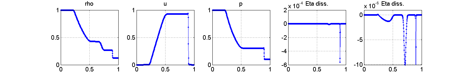
Figure 1: Sod’s 1D shock tube problem discrete solution at time $T=0.23$. Number of cells: 400.

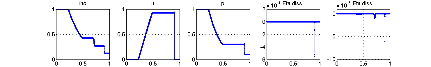
Figure 2: Sod’s 1D shock tube problem discrete solution at time $T=0.23$. Number of cells: 4000.

4 Concluding remarks and perspectives

In this paper, we have justified the new family of Lagrange-flux schemes from the point of view of the discrete entropy stability property. We have found pseudo-viscosity terms that return an entropy production at the right order of magnitude for a semi-discretized version of Lagrange-Flux schemes. Even if further analysis is needed (multidimensional extension, analysis of the full space-time discretized scheme), we believe that Lagrange-flux schemes are very promising because of their generic formulation, simplicity of implementation, simple expressions of numerical fluxes, flexibility for achieving higher-order accuracy, HPC performance (see the references below), and flexibility for multiphysics coupling.

- (1) Braeunig, J.P.: Reducing the entropy production in a collocated Lagrange-Remap scheme. Journal of Computational Physics 314, 127–144 (2016)
- (2) De Vuyst, F., Béchereau, M., Gasc, M., Motte, R., Peybernes, M., Poncet, R.: Stable and accurate low-diffusive interface capturing advection schemes (2016). URL https://arxiv.org/abs/1605.07091. ArXiv Preprint arXiv:1605.07091v1
- (3) De Vuyst, F., Gasc, T., Motte, R., Peybernes, M., Poncet, R.: Lagrange-Flux Eulerian schemes for compressible multimaterial flows. In: Proc. of the ECCOMAS Congress 2016, VII Eur. Congress on Comp. Meth. in Appl. Sci. and Eng., Crete Island, Greece, pp. 1165–1178 (2016)
- (4) De Vuyst, F., Gasc, T., Motte, R., Peybernes, M., Poncet, R.: Lagrange-Flux schemes: Reformulating second-order accurate Lagrange-Remap schemes for better node-based HPC performance. Oil and Gas Science and Technology journal (OGST) 71(6) (2016)
- (5) Després, B., Mazeran, C.: Lagrangian Gas Dynamics in two dimensions and Lagrangian systems. Archive for Rational Mechanics and Analysis 178, 327–372 (2005)
- (6) Gasc., T.: Modèles de performance pour l’adaptation des méthodes numériques aux architectures multi-cœurs vectorielles. Application aux schémas Lagrange-projection en hydrodynamique compressible. PhD dissertation, ENS Paris-Saclay, Université Paris-Saclay (2016)
- (7) Godlewski, E., Raviart, P.A.: Numerical approximation of hyperbolic systems of conservation laws, Applied Mathematical Sciences, vol. 118. Springer-Verlag, New York (1996)
- (8) Maire, P.H., Abgrall, R., Breil, J., Ovadia, J.: A cell-centered Lagrangian scheme for two-dimensional compressible flow problems. SIAM J. on Sci. Comp. 29, 1781–1824 (2007)
- (9) Poncet, R., Peybernes, M., Gasc, T., De Vuyst, F.: Performance modeling of a compressible hydrodynamics solver on multicore CPUs, Advances in parallel computing, vol. 27: Parallel Computing: on the road to Exascale. IOS Press Ebook, New York (2016)
- (10) Toro, E.F.: Riemann solvers and numerical methods for Fluid Dynamics. Springer (2009)