The independent loss model with ordered insertions for the evolution of CRISPR spacers

Abstract

Today, the CRISPR (clustered regularly interspaced short palindromic repeats) region within bacterial and archaeal genomes is known to encode an adaptive immune system. We rely on previous results on the evolution of the CRISPR arrays, which led to the ordered independent loss model, introduced by Kupczok and Bollback (2013). When focusing on the spacers (between the repeats), new elements enter a CRISPR array at rate $\theta$ at the leader end of the array, while all spacers present are lost at rate $\rho$ along the phylogeny relating the sample. Within this model, we compute the distribution of distances of spacers which are present in all arrays in samples of size $n=2$ and $n=3$. We use these results to estimate the loss rate $\rho$ from spacer array data.

1 Introduction

The CRISPR Cas system is a widespread microbial adaptive defense mechanism against viruses and plasmids (Marraffini, 2015; Rath et al., 2015), that likely originated in archaea and spread to bacteria via horizontal transfer (Makarova et al., 2011a). The Clustered Regulary Interspaced Short Palindromic Repeats (CRISPR) have already been described in 1987 by Ishino et al. (1987). Later it turned out that the unique sequences between these repeats, so called spacers, are of foreign origin (Bolotin et al., 2005) and serve as an immunological memory passed to the offspring. New spacers are acquired and inserted at the leader end of the array (Barrangou et al., 2007), such that the order of spacers represents the chronological infection history of the bacterial population. Together with CRISPR associated (cas) genes these spacers can provide resistance against phages and plasmids by targeting molecular scissors to the corresponding sequences in the invading DNA (Barrangou et al., 2007).

The most prominent cas gene is Cas9, which recently led to a revolution in genome engineering (Doudna and Charpentier, 2014; Hsu et al., 2014). With the CRISPR-Cas9 enzyme mechanism an uncomplicated and cheap technology to alter the genome of potentially any organism is now available. Due to the precise targeting via engineered spacer sequences this system is speeding up the pace of research and gives rise to applications with incredible impact and opportunities in a variety of fields (Doudna and Charpentier, 2014). As just one among many examples, the concept of gene drive (Burt, 2003) in combination with the precision of CRISPR-Cas9 may enable us to alter the genetics of entire populations (Esvelt et al., 2014; Oye et al., 2014).

Here we will focus on the evolution of natural CRISPR-Cas systems and their spacer arrays in microbial genomes. CRISPR systems have been classified into different types and subtypes, with different sets of accompanying cas genes (Makarova et al., 2011b, 2015). A single genome can contain different types of CRISPR and the rates at which new spacers are inserted and old spacers are lost vary between the systems (Horvath et al., 2008). This suggests that different types may have different evolutionary dynamics and functions beyond defense, e.g. in regulation of gene expression (Westra et al., 2014). As another example, Lopez-Sanchez et al. (2012) suggest that CRISPR may control the diversity of mobile genetic elements in Streptococcus agalactiae.

So far we just got a glimpse of the ecological and evolutionary impact of CRISPR cas systems. In particular, the benefit of possessing a CRISPR system and the parameter regime where they are maintained (Levin, 2010; Weinberger et al., 2012), as well as the coevolutionary dynamics of bacteria containing CRISPR loci and phages (Koskella and Brockhurst, 2014; Han and Deem, 2017) have been considered. However many ecological and evolutionary aspects of CRISPR cas systems, as the frequent horizontal transfer of the whole system, are still not understood (Rath et al., 2015). Not only the evolution of the whole CRISPR system but the evolving and adapting spacer array itself is of interest. The spacer array represents snippets of previous phage/plasmid exposure that can help to disentangle the interplay between bacterial and viral populations (Childs et al., 2014; Sun et al., 2015). Since resistance is inherited by the offspring via the acquired spacer sequences, at least some CRISPR systems blur the distinction between Darwinian and Lamarckian modes of evolution (Koonin and Wolf, 2016). Modeling the evolution of spacer arrays will help to identify differences between CRISPR types and interpret the observed pattern of spacer insertion and deletion.

In 2013, Kupczok and Bollback introduced probabilistic models for the evolution of CRISPR spacer arrays. They concluded that a model with ordered spacer insertions and independent losses best describes the dynamics of spacer array evolution. In this model unique new spacers are inserted at the leader end and each spacer gets lost independently at a constant rate; see also Definition 2.1 below. Later, the model has been extended to conclude that there is no evidence for frequent recombination within the spacer arrays (Kupczok et al., 2015). In Kupczok and Bollback (2013) the constructed estimators for spacer insertion and deletion rates assume that no phylogenetic information is available. In contrast, in this paper we assume that the genealogy is known or has been reconstructed adequately, e.g. based on the cas genes in front of the spacer array. Given such a genealogy we look at distances between equal spacers, i.e. spacers that appear in more than one array. Kupczok and Bollback (2013) also considered an unordered independent loss model, where the order of spacers is irrelevant. In pangenome analysis (Mira et al., 2010; Vernikos et al., 2014), this model is known as the infinitely many genes model (Baumdicker et al., 2010) and has led to methods to jointly estimate gene gain and loss rates based on the frequency of genes in the sample (Baumdicker et al., 2012). These methods can directly be applied in our setting to jointly infer the rates of spacer insertion and deletion from (unordered) spacer frequencies. Here we compute the distribution of distances of (ordered) spacers, which are present in all arrays in samples of size $n=2$ and $n=3$. We show that including the order of spacer arrays by looking at equal spacer distances in a sample of arrays allows to decouple estimation of spacer insertion and spacer loss rate.

The paper is organized as follows: In Section 2, we introduce the ordered independent loss model. In Section 3, we compute the distribution of equal spacer distances of samples of size $n=2$ and $n=3$. As a by-product, we find sufficient statistics useful for the estimation of the loss rate. These are employed in Section 4 where we give maximum likelihood estimators and perform simulations in order to show their accuracy.

2 Model

The following model for the evolution of spacers in the CRISPR-system is based on work by Kupczok and Bollback (2013). Since this model was called the ordered model with independent losses, we follow this terminology here.

Definition 2.1 (The ordered independent loss model along a single line).

Let $\mathcal{S}=(S_{t})_{t\geq 0}$ be a Markov jump process with state space $E=[0,1]^{\mathbb{N}}$ and the following dynamics: If $S(t)=s=(s_{1},s_{2},\dots)$, it jumps to

$$(U,s_{1},s_{2},\dots) \text{ at rate }\theta\text{ for some independent, uniform $U\in[0,1]$},$$

$$(s_{1},\dots,s_{i-1},s_{i+1},s_{i+2},\dots) \text{ at rate }\rho\text{ for each $i=1,2,\dots$}$$

The first type is called a gain-event (or insertion event), while the latter is called a loss-event (or deletion event). We refer to $S$ as the independent loss model with ordered gains, or as the ordered independent loss model, for short.

A simple result is the following, which is clear from the definition of $\mathcal{S}$.

Lemma 2.2 (Equilibrium of $S$).

Let $(U_{1},U_{2},\dots)\in E$ be a sequence of independent, $U([0,1])$-distributed random variables. Then, the distribution $\pi$ of $(U_{1},U_{2},\dots)$ is an equilibrium of $\mathcal{S}$ from Definition 2.1.

Remark 2.3 (More equilibria).

We note that $\pi$ is not the only equilibrium of the process. For example, let $N\sim\text{Poi}(\theta/\rho)$ and, conditioned on $N$, let $(V_{1},\dots,V_{N})$ be independent and $U([0,1])$-distributed, and $V_{N+1}=V_{N+2}=\cdots=1$. Then, the distribution of $(V_{1},V_{2},\dots)$ is stationary for $S$ as well.
Indeed, let $N_{t}:=\sup\{n:U_{1},\dots,U_{n}\notin S(0)\}$. Then, $\mathcal{N}=(N_{t})_{t\geq 0}$ is a death-immigration process with immigration rate $\theta$ and, if it is in state $n$, death rate $n\rho$. For this process, it is well-known that $N_{t}\xRightarrow{t\to\infty}N$; hence, necessarily, $V_{1},\dots,V_{N}$ are independent and uniform draws from $[0,1]$ for a stationary distribution. However, $V_{N+1},V_{N+2},\dots$ are states also found in $S(0)$, so if $S(0)=(1,1,\dots)$, then $S_{N_{t}+k}(t)=1$ for all $t$ and $k$ by construction.

In order to formulate our results, we require the ordered independent loss model not only along a single line, but also along an ultra-metric tree. For this, we introduce some notation.

Remark 2.4 (Ultrametric trees; tree-indexed processes).

1. Recall that a tree $\mathbbm{T}$ with leaves $\mathbbm{L}\subseteq\mathbbm{T}$ is called ultra-metric if $d(\ell_{1},\ell_{3})\leq\max(d(\ell_{1},\ell_{2}),d(\ell_{2},\ell_{3}))$ for all $\ell_{1},\ell_{2},\ell_{3}\in\mathbbm{L}$. Here, $d(.,.)$ denotes the graph distance and $\ell\in\mathbbm{T}$ is a leaf if $\mathbbm{T}\setminus\{\ell\}$ only has a single connected component. Note that for such an ultra-metric tree there is a unique $r\in\mathbbm{T}$ (called the root) such that $d(r,\ell)$ does not depend on $\ell\in\mathbbm{L}$. In addition, there is an order on $\mathbbm{T}$ such that $s\leq t$ iff $s\in[r,t]$, where $[r,t]$ is the unique path from $r$ to $t$. Then, we also say that $s$ is ancestor of $t$. Using this order the most recent common ancestor $s\wedge t\in\mathbbm{T}$ of $s$ and $t$ is the largest element in $\mathbbm{T}$ which is ancestor of both, $s$ and $t$.

2. Usually, a Markov process $X=(X_{t})_{t\geq 0}$ has the property that $(X_{t})_{t\geq s}$ is independent of $(X_{t})_{t\leq s}$ conditional on $X_{s}$. Moreover, we call a Markov-process time-homogeneous if there is a family of transition kernels $(p_{s}(.,.))_{s\geq 0}$ such that

   $$\mathbf{P}(X_{t}\in A|X_{r}=x)=p_{t-r}(x,A)\text{ for all }r\leq t.$$ (2.1)

   If a Markov-process is piecewise constant, it is usually called a Markov jump process. If it is time-homogeneous, it follows from (2.1) that the waiting time to the next jump has an exponential distribution. Its parameter depends on the current state and is usually referred to as the rate of the exponential distribution. We call a tree-indexed process $X=(X_{t})_{t\in\mathbbm{T}}$ time-homogeneous Markov if (2.1) holds for all $r,t\in\mathbbm{T}$ with $r\leq t$, where $t-r:=d(r,t)$, and, conditional on the value of the process at a node, the processes in the two descending subtrees are independent. For more work on Markov processes indexed by trees, see e.g. Benjamini and Peres (1994).

Definition 2.5 (The ordered independent loss model along an ultrametric tree).

Let $\mathbbm{T}$ be an ultra-metric tree with root $r\in\mathbbm{T}$. The $\mathbbm{T}$-indexed time-homogeneous Markov process $\mathcal{S}=(S_{t})_{t\in\mathbbm{T}}$ with $S_{r}\sim\pi$ (recall from Lemma 2.2) and transition kernels given through gain and loss events as in Definition 2.1, is denoted the ordered independent loss model (along $\mathbbm{T}$).

Remark 2.6.

Note that it is straightforward to formulate the presented results for non-ultrametric trees. However, since the formulas simplify significantly for ultrametric trees, we assume that $\mathbb{T}$ is ultrametric.

In the sequel, we fix the ultra-metric tree $\mathbbm{T}$, its set of leaves $\mathbbm{L}$ and the process $\mathcal{S}$ from Definition 2.5. Recall that $S_{t}\in[0,1]^{\mathbbm{N}}$ and we will use the shorthand notation

$$S_{t,i}:=(S_{t})_{i}.$$

Moreover, we will identify the vector $S_{t}$ with the set of its entries, i.e. $S_{t}=\{S_{t,i}:i=1,2,\dots\}$. Note that all entries of $S_{t}$ are different almost surely.

Definition 2.7 (Equal spacers).

For $\mathbbm{K}\subseteq\mathbbm{L}$ and $\ell\in\mathbbm{K}$, define recursively

$$E^{\ell,\mathbbm{K}}_{0} :=E^{\ell,\mathbbm{K},(\mathbbm{L})}_{0}:=0,$$

$$E^{\ell,\mathbbm{K}}_{n+1} :=E^{\ell,\mathbbm{K},(\mathbbm{L})}_{n+1}:=\min\Big{\{}i>E^{\ell,\mathbbm{K}}_{n}:S_{\ell,i}\in\bigcap_{k\in\mathbbm{K}}S_{k}\setminus\Big{(}\bigcup_{k^{\prime}\in\mathbbm{L}\setminus\mathbbm{K}}S_{k^{\prime}}\Big{)}\Big{\}},\qquad n=1,2,\dots$$

Here, $E^{\ell,\mathbbm{K}}_{n}$ is the spacer position in $\ell$ of the $n$th spacer which is also contained in all $S_{k},k\in\mathbbm{K}$, but in none of $S_{k^{\prime}},k^{\prime}\in\mathbbm{L}\setminus\mathbbm{K}$.

An illustration of the process from Definition 2.5 and the corresponding equal spacers are shown in Figure 2.1.

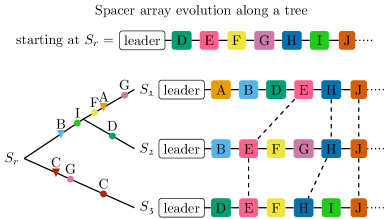
Figure 2.1: Illustration of the ordered independent loss model along a tree from Definition 2.5. New spacers (A-C) are inserted at the leader position at rate $\theta$ along the branches, marked by $\blacktriangledown$. Present spacers (A-J $\cdots$) are lost at rate $\rho$, marked by $\bullet$. Dashed lines connect the first three equal spacers shared between all arrays. Here $\mathbbm{L}=\{\mathfrak{1},\mathfrak{2},\mathfrak{3}\}$ and from Definition 2.7 we get, $E_{1}^{\mathfrak{2},\mathbbm{L}}=E_{1}^{\mathfrak{3},\mathbbm{L}}=2$, $E_{1}^{\mathfrak{1},\mathbbm{L}}=E_{2}^{\mathfrak{3},\mathbbm{L}}=4$, $E_{2}^{\mathfrak{1},\mathbbm{L}}=E_{2}^{\mathfrak{2},\mathbbm{L}}=5$ and $E_{3}^{\mathfrak{1},\mathbbm{L}}=E_{3}^{\mathfrak{2},\mathbbm{L}}=E_{3}^{\mathfrak{3},\mathbbm{L}}=6$.

3 Results

3.1 Trees with two leaves $|\mathbbm{L}|=2$

In the special case that $\mathbbm{L}$ consists of only two points, we denote these leaves by $\mathfrak{1}$ and $\mathfrak{2}$. In addition, we set $d(\mathfrak{1},\mathfrak{2})=2T$ for some $T\geq 0$ and define the following random variables:

$$V_{i} :=E_{i}^{\mathfrak{1},\{\mathfrak{1},\mathfrak{2}\}},\qquad W_{i}:=E_{i}^{\mathfrak{2},\{\mathfrak{1},\mathfrak{2}\}},\qquad i=1,2,\dots,$$

i.e. $V_{i}$ is the $i$th element of $S_{\mathfrak{1}}$ which is also contained in $S_{\mathfrak{2}}$ and $W_{i}$ is the $i$th element of $S_{\mathfrak{2}}$ which is also contained in $S_{\mathfrak{1}}$.

Theorem 1 (Distribution of equal spacer sequence in two leaves).

Let $(A,B),(A_{1},B_{1}),(A_{2},B_{2}),\dots$ be iid pairs of random variables with joint distribution

$$\mathbb{P}(A=a,B=b) =\binom{a+b}{a}\cdot\frac{e^{-\rho T}}{2-e^{-\rho T}}\cdot\bigg{(}\frac{1-e^{-\rho T}}{2-e^{-\rho T}}\bigg{)}^{a+b}$$ (3.1)

In addition, let $C_{\mathfrak{1}},C_{\mathfrak{2}}$ be iid Poisson distributed r.v. with parameter $\frac{\theta}{\rho}(1-e^{-\rho T})$. Then,

$$(V_{1},W_{1}),(V_{2}-V_{1},W_{2}-W_{1}),(V_{3}-V_{2},W_{3}-W_{2}),\dots$$

are independent with

$$(V_{1},W_{1})\sim(C_{\mathfrak{1}}+A_{1},C_{\mathfrak{2}}+B_{1}),\qquad(V_{i}-V_{i-1},W_{i}-W_{i-1})\sim(A_{i},B_{i}),\qquad i=2,3,\dots$$

Remark 3.1 ($A$ and $B$ are geometrically distributed).

1. In the sequel, we will use the identity

   $$\sum_{b=0}^{\infty}\binom{a+b}{a}x^{b}=\frac{1}{(1-x)^{a+1}},\qquad i=0,1,2,\dots$$ (3.2)

   for $|x|<1$ on several occasions. It can easily be proven by induction.

2. For the distribution of $(A,B)$ from (3.1), we note that both, $A$ and $B$ are geometrically distributed with parameter $e^{-\rho T}$. (We come back to this observation in Remark 3.3.)
   Indeed: For

   $$x=\frac{1-e^{-\rho T}}{2-e^{-\rho T}}=1-\frac{1}{2-e^{-\rho T}},$$ (3.3)

   we have that

   $$\mathbbm{P}(A=a) =\frac{e^{-\rho T}}{2-e^{-\rho T}}\sum_{b=0}^{\infty}\binom{a+b}{a}x^{a+b}=\frac{e^{-\rho T}}{2-e^{-\rho T}}\frac{1}{1-x}\Big{(}\frac{x}{1-x}\Big{)}^{a}=e^{-\rho T}(1-e^{-\rho T})^{a}.$$

   So, we have shown that $A$ has the desired distribution. Symmetry then gives the same for $B$.

Before we come to the proof of Theorem 1, we state the sampling formula which results from Theorem 1.

Corollary 3.2 (Sampling formula for equal spacer sequence in two leaves).

The joint distribution of $(V_{1},V_{2},\dots,V_{m},W_{1},W_{2},\dots,W_{m})$ is given by

$$\mathbbm{P}( V_{1}=v_{1},\dots,V_{m}=v_{m},W_{1}=w_{1},\dots,W_{m}=w_{m})$$

$$=\bigg{(}\Big{(}\frac{\theta}{\rho}(1-e^{-\rho T})\Big{)}^{v_{1}+w_{1}}e^{-2\frac{\theta}{\rho}(1-e^{-\rho T})}\,\frac{e^{-\rho T}}{2-e^{-\rho T}}$$

$$\qquad\cdot\sum_{v=0}^{v_{1}}\sum_{w=0}^{w_{1}}\binom{v+w}{v}\frac{1}{(v_{1}-v)!(w_{1}-w)!}\frac{1}{(\frac{\theta}{\rho}(2-e^{-\rho T}))^{v+w}}\bigg{)}$$

$$\qquad\qquad\cdot\bigg{(}\prod_{i=2}^{m}\binom{\Delta v_{i}+\Delta w_{i}}{\Delta v_{i}}\bigg{)}\cdot\bigg{(}\frac{e^{-\rho T}}{2-e^{-\rho T}}\bigg{)}^{m-1}\cdot\bigg{(}\frac{1-e^{-\rho T}}{2-e^{-\rho T}}\bigg{)}^{\sum_{i=2}^{m}\Delta v_{i}+\Delta w_{i}}$$

for $m=1,2,\dots$, where $\Delta v_{i}:=v_{i}-v_{i-1},\Delta w_{i}:=w_{i}-w_{i-1},i=2,3,\dots$

Proof.

By the independence from Theorem 1 and the distribution given in (3.1), the only thing which remains to be proven is that

$$\mathbbm{P}(V_{1}=v_{1},W_{1}=w_{1}) =\Big{(}\frac{\theta}{\rho}(1-e^{-\rho T})\Big{)}^{v_{1}+w_{1}}e^{-2\frac{\theta}{\rho}(1-e^{-\rho T})}\,\frac{e^{-\rho T}}{2-e^{-\rho T}}$$

$$\qquad\qquad\qquad\cdot\sum_{a=0}^{v_{1}}\sum_{b=0}^{w_{1}}\binom{a+b}{a}\frac{1}{(v_{1}-a)!(w_{1}-b)!}\frac{1}{(\frac{\theta}{\rho}(2-e^{-\rho T}))^{a+b}}.$$

From Theorem 1, we know that $(V_{1},W_{1})\sim(C_{\mathfrak{1}}+A,C_{\mathfrak{2}}+B)$, where the distribution of $(A,B)$ is as in (3.1) and $C_{\mathfrak{1}}$ and $C_{\mathfrak{2}}$ are independent and Poisson distributed with mean $z:=\frac{\theta}{\rho}(1-e^{-\rho T})$. Hence, with $x$ from (3.3),

$$\mathbbm{P}( V_{1}=v_{1},W_{1}=w_{1})=\sum_{a=0}^{v_{1}}\sum_{b=0}^{w_{1}}\mathbbm{P}(A=a,C_{\mathfrak{1}}=v_{1}-a,B=b,C_{\mathfrak{2}}=w_{1}-b)$$

$$=\sum_{a=0}^{v_{1}}\sum_{b=0}^{w_{1}}\mathbbm{P}(A=a,B=b)\cdot\mathbbm{P}(C_{\mathfrak{1}}=v_{1}-a)\cdot\mathbbm{P}(C_{\mathfrak{2}}=w_{1}-b)$$

$$=\sum_{v=0}^{v_{1}}\sum_{w=0}^{w_{1}}\binom{a+b}{a}\frac{e^{-\rho T}}{2-e^{-\rho T}}x^{a+b}\frac{z^{v_{1}+w_{1}-(a+b)}}{(v_{1}-a)!(w_{1}-b)!}e^{-2z}$$

$$=z^{v_{1}+w_{1}}\frac{e^{-2z}e^{-\rho T}}{2-e^{-\rho T}}\sum_{a=0}^{v_{1}}\sum_{b=0}^{w_{1}}\binom{a+b}{a}\frac{1}{(v_{1}-a)!(w_{1}-b)!}\Big{(}\frac{x}{z}\Big{)}^{a+b}.$$

Plugging in $x$ and $z$ gives the result. ∎

Proof of Theorem 1.

For the leaves $\mathfrak{1}$ and $\mathfrak{2}$, recall that $\mathfrak{1}\wedge\mathfrak{2}$ denotes their MRCA (most recent common ancestor) and $d(\mathfrak{1},\mathfrak{1}\wedge\mathfrak{2})=T$. Let $C_{\mathfrak{1}}(C_{\mathfrak{2}})$ be the number of gain-events between $\mathfrak{1}\wedge\mathfrak{2}$ and $\mathfrak{1}$ ($\mathfrak{2}$), which don’t get lost until $\mathfrak{1}$ (until $\mathfrak{2}$). Then, by construction, $C_{\mathfrak{1}}$ and $C_{\mathfrak{2}}$ are independent (since they depend on independent gain events) and Poisson distributed with mean

$$\int_{0}^{T}\theta e^{-\rho t}dt=\frac{\theta}{\rho}(1-e^{-\rho T}).$$

For $(S_{\mathfrak{1},C_{\mathfrak{1}}+i})_{i=1,2,\dots}$ and $(S_{\mathfrak{2},C_{\mathfrak{2}}+i})_{i=1,2,\dots}$, i.e. the spacers after the just mentioned gain-events, we note that, by construction,

$$\{S_{\mathfrak{1},C_{\mathfrak{1}}+i}:i=1,2,\dots\}\cup\{S_{\mathfrak{2},C_{\mathfrak{2}}+i}:i=1,2,\dots\}\subseteq S_{\mathfrak{1}\wedge\mathfrak{2}}.$$

Moreover, we have that (by independence of loss-events at all positions) the events

$$(\{s\in S_{\mathfrak{1}}\},\{s\in S_{\mathfrak{2}}\})_{s\in S_{\mathfrak{1}\wedge\mathfrak{2}}}$$

are independent with

$$\mathbbm{P}(s\in S_{\mathfrak{1}})=\mathbbm{P}(s\in S_{\mathfrak{2}})=e^{-\rho T}$$

for all $s\in S_{\mathfrak{1}\wedge\mathfrak{2}}$. Equivalently, we find that independently for all $s\in S_{\mathfrak{1}\wedge\mathfrak{2}}$,

$$p_{1} :=\mathbbm{P}(s\in S_{\mathfrak{1}}\setminus S_{\mathfrak{2}})=e^{-\rho T}(1-e^{-\rho T}),$$ (3.4)

$$p_{2} :=\mathbbm{P}(s\in S_{\mathfrak{2}}\setminus S_{\mathfrak{1}})=e^{-\rho T}(1-e^{-\rho T}),$$

$$p_{3} :=\mathbbm{P}(s\notin S_{\mathfrak{2}}\cup S_{\mathfrak{1}})=(1-e^{-\rho T})^{2},$$

$$p_{4} :=\mathbbm{P}(s\in S_{\mathfrak{2}}\cap S_{\mathfrak{1}})=e^{-2\rho T}.$$

Moving along $S_{\mathfrak{1}\wedge\mathfrak{2}}$, toss a four-sided die, numbered $1,\dots,4$. If it comes up 1, keep the spacer in $\mathfrak{1}$ but not in $\mathfrak{2}$; if it comes up 2, keep it in $\mathfrak{2}$ but not in $\mathfrak{1}$; if it comes up 3, neither keep it in $\mathfrak{1}$ nor in $\mathfrak{2}$; if it comes up 4, keep it in both, $\mathfrak{1}$ and $\mathfrak{2}$. Then, we need to compute the joint distribution of the number of die rolls $A$ with 1 and $B$ with 2 before the first 4 (which indicates an equal spacer). Letting $K$ be the first die roll with 4, we have that

$$\mathbbm{P} (A=a,B=b)=\sum_{k=a+b+1}^{\infty}\mathbbm{P}(A=a,B=b,K=k)$$

$$=\sum_{k=a+b+1}^{\infty}\mathbbm{P}(K=k)\mathbbm{P}(A=a,B=b|K=k)$$

$$=\sum_{k=a+b+1}^{\infty}p_{4}(1-p_{4})^{k-1}\binom{k-1}{a+b}\binom{a+b}{a}\left(\frac{p_{1}}{1-p_{4}}\right)^{a}\left(\frac{p_{2}}{1-p_{4}}\right)^{b}\left(\frac{p_{3}}{1-p_{4}}\right)^{k-1-(a+b)}$$

$$=\binom{a+b}{a}p_{1}^{a}p_{2}^{b}p_{4}\sum_{k=a+b+1}^{\infty}\binom{k-1}{a+b}p_{3}^{k-1-(a+b)}$$

$$=\binom{a+b}{a}p_{1}^{a}p_{2}^{b}p_{4}\sum_{k=0}^{\infty}\binom{a+b+k}{a+b}p_{3}^{k}$$

$$=\binom{a+b}{a}\frac{p_{4}}{1-p_{3}}\Big{(}\frac{p_{1}}{1-p_{3}}\Big{)}^{a+b}$$

$$=\binom{a+b}{a}\frac{e^{-2\rho T}}{1-(1-e^{-\rho T})^{2}}\Big{(}\frac{e^{-\rho T}(1-e^{-\rho T})}{1-(1-e^{-\rho T})^{2}}\Big{)}^{a+b}$$

$$=\binom{a+b}{a}\frac{e^{-\rho T}}{2-e^{-\rho T}}\Big{(}\frac{1-e^{-\rho T}}{2-e^{-\rho T}}\Big{)}^{a+b}$$

since $p_{1}=p_{2}$, where we have used (3.2) in the second to last equality. Before the first equal spacer, we have for $(V_{1},W_{1})$ the sum of new and old spacers, while for $(V_{i},W_{i}),i\geq 1$, we only have old spacers. Since loss events of spacers in $\mathfrak{1}\wedge\mathfrak{2}$ are independent, the result follows. ∎

Remark 3.3 ($\Delta V_{i}$ and $\Delta W_{i}$ are geometrically distributed).

We have seen in the proof of Theorem 1 that the distribution of $(\Delta V_{i},\Delta W_{i})$ for $i=2,3,\dots$ can be obtained by rolling a die with probabilities $p_{1},\dots,p_{4}$ given by (3.4) and counting the number of occurrences of 1 and 2 before the first 4. For the marginal distribution of $\Delta V_{i}$, we are asking for the number of occurrences of 1 before the first 4. Clearly, this is geometrically distributed with success probability $p_{4}/(p_{1}+p_{4})=e^{-\rho T}$. See also the formal calculation in Remark 3.1.

3.2 Trees with three leaves $|\mathbbm{L}|=3$

In the special case that $\mathbbm{L}$ consists of three points, denoted $\mathfrak{1},\mathfrak{2}$ and $\mathfrak{3}$, we define the following random variables:

$$X_{i} :=E_{i}^{\mathfrak{1},\{\mathfrak{1},\mathfrak{2},\mathfrak{3}\}},\qquad Y_{i}:=E_{i}^{\mathfrak{2},\{\mathfrak{1},\mathfrak{2},\mathfrak{3}\}},\qquad Z_{i}:=E_{i}^{\mathfrak{3},\{\mathfrak{1},\mathfrak{2},\mathfrak{3}\}},\qquad i=0,1,2,\dots,$$

i.e. $X_{i}$ is the $i$th element of $S_{\mathfrak{1}}$ which is also contained in both, $S_{\mathfrak{2}}$ and $S_{\mathfrak{3}}$, $Y_{i}$ is the $i$th element of $S_{\mathfrak{2}}$ which is also contained in $S_{\mathfrak{1}}$ and $S_{\mathfrak{3}}$, and $Z_{i}$ is the $i$th element of $S_{\mathfrak{3}}$ which is also contained in $S_{\mathfrak{1}}$ and $S_{\mathfrak{2}}$. In between $X_{i}$ and $X_{i+1}$, for example, we find spacers of three classes: those, which are only in $S_{\mathfrak{1}}$, i.e. in $S_{\mathfrak{1}}\setminus(S_{\mathfrak{2}}\cup S_{\mathfrak{3}})$, those which are shared with $S_{\mathfrak{2}}$, i.e. in $S_{\mathfrak{1}}\cap S_{\mathfrak{2}}\setminus S_{\mathfrak{3}}$, and those shared with $S_{\mathfrak{3}}$, i.e. in $S_{\mathfrak{1}}\cap S_{\mathfrak{3}}\setminus S_{\mathfrak{2}}$. Recalling the notation from Definition 2.7, we write for $\mathbbm{K}\subseteq\mathbbm{L}=\{\mathfrak{1},\mathfrak{2},\mathfrak{3}\}$

$$F_{i}^{\mathbbm{K}} :=\#\{E_{i}^{k,\mathbbm{L}},E_{i}^{k,\mathbbm{L}}\!\!+\!1,\dots,E_{i+1}^{k,\mathbbm{L}}\}\cap\{E_{n}^{k,\mathbbm{K}}:n=1,2,\dots\},\qquad i=0,1,2,...$$

where the right hand side does not depend on which $k\in\mathbbm{K}$ we choose, because the order is not altered by losses. In words, $F_{i}^{\mathbbm{K}}$ is the number of spacers within $S_{k}$, which are between the $i$th and $(i+1)$st spacer shared among $\mathfrak{1},\mathfrak{2},\mathfrak{3}$ and that appear in all elements of $\mathbbm{K}$, but in no element of $\mathbbm{L}\setminus\mathbbm{K}$. As an example, we can rewrite

$$F_{i}^{\{\mathfrak{1}\}} =\#\{S_{\mathfrak{1},X_{i}},S_{\mathfrak{1},X_{i}+1},\dots,S_{\mathfrak{1},X_{i+1}}\}\cap(S_{\mathfrak{1}}\setminus(S_{\mathfrak{2}}\cup S_{\mathfrak{3}})),$$

$$F_{i}^{\{\mathfrak{1},\mathfrak{2}\}} =\#\{S_{\mathfrak{1},X_{i}},S_{\mathfrak{1},X_{i}+1},\dots,S_{\mathfrak{1},X_{i+1}}\}\cap((S_{\mathfrak{1}}\cap S_{\mathfrak{2}})\setminus S_{\mathfrak{3}}),$$

$$=\#\{S_{\mathfrak{2},Y_{i}},S_{\mathfrak{2},Y_{i}+1},\dots,S_{\mathfrak{2},Y_{i+1}}\}\cap((S_{\mathfrak{1}}\cap S_{\mathfrak{2}})\setminus S_{\mathfrak{3}}).$$

Note that $X_{i+1}-X_{i}=F_{i}^{\mathfrak{1}\setminus(\mathfrak{2},\mathfrak{3})}+F_{i}^{(\mathfrak{1}\cup\mathfrak{2})\setminus\mathfrak{3}}+F_{i}^{(\mathfrak{1}\cup\mathfrak{3})\setminus\mathfrak{2}}+1$ by construction, $i=0,1,2,\dots$

Since there is exactly one tree topology of a tree with three leaves, we will pick an ultra-metric tree, where $\mathfrak{1}$ and $\mathfrak{2}$ are closer relatives than $\mathfrak{1}$ and $\mathfrak{3}$ (and therefore also closer than $\mathfrak{2}$ and $\mathfrak{3}$). So, $T,T^{\prime}$ denote the distances from $\mathfrak{1}$ to $\mathfrak{3}$ and from $\mathfrak{1}$ to $\mathfrak{2}$, respectively, with $T\geq T^{\prime}$. See Figure 3.1 for an illustration of the tree topology.

Figure 3.1: The tree topology for three leaves is chosen such that $\mathfrak{1},\mathfrak{2}$ are closer related than $\mathfrak{1},\mathfrak{3}$ and $\mathfrak{2},\mathfrak{3}$.

Theorem 2 (Distribution of equal spacer sequence in three leaves).

For $\mathbbm{L}=\{\mathfrak{1},\mathfrak{2},\mathfrak{3}\}$, let $(A^{\mathbbm{K}})_{\emptyset\subsetneq\mathbbm{K}\subsetneq\mathbbm{L}},(A_{1}^{\mathbbm{K}})_{\emptyset\subsetneq\mathbbm{K}\subsetneq\mathbbm{L}},(A_{2}^{\mathbbm{K}})_{\emptyset\subsetneq\mathbbm{K}\subsetneq\mathbbm{L}},\dots$ be iid tuples of random variables with joint distribution

$$P(A^{\{\mathfrak{1}\}}=a,A^{\{\mathfrak{2}\}}=b,A^{\{\mathfrak{3}\}}=c,A^{\{\mathfrak{1},\mathfrak{2}\}}=d,A^{\{\mathfrak{1},\mathfrak{3}\}}=e,A^{\{\mathfrak{2},\mathfrak{3}\}}=f)$$ (3.5)

$$=\binom{a+b+c+d+e+f}{a,b,c,d,e,f}\Big{(}\frac{(1-e^{-\rho T})(1-e^{-\rho T^{\prime}})}{r}\Big{)}^{a+b}\Big{(}\frac{1-2e^{-\rho T}+e^{-\rho(T+T^{\prime})})}{r}\Big{)}^{c}$$

$$\qquad\qquad\qquad\qquad\qquad\qquad\cdot\Big{(}\frac{e^{-\rho T^{\prime}}(1-e^{-\rho T})}{r}\Big{)}^{d}\Big{(}\frac{e^{-\rho T}(1-e^{-\rho T^{\prime}})}{r}\Big{)}^{e+f}\frac{e^{-\rho T}e^{-\rho T^{\prime}}}{r}$$

with

$$r:=3-e^{-\rho T^{\prime}}-e^{-\rho T}(2-e^{-\rho T^{\prime}}).$$

In addition, let

$$C^{\{\mathfrak{1}\}}\stackrel{{\scriptstyle d}}{{=}}\text{Poi}\left(\frac{\theta}{\rho}(1-e^{-\rho T^{\prime}})(1+e^{-\rho T^{\prime}}-e^{-\rho T})\right), C^{\{\mathfrak{1},\mathfrak{2}\}}\stackrel{{\scriptstyle d}}{{=}}\text{Poi}\left(\frac{\theta}{\rho}(1-e^{-\rho(T-T^{\prime})})e^{-2\rho T^{\prime}}\right),$$

$$C^{\{\mathfrak{2}\}}\stackrel{{\scriptstyle d}}{{=}}\text{Poi}\left(\frac{\theta}{\rho}(1-e^{-\rho T^{\prime}})(1+e^{-\rho T^{\prime}}-e^{-\rho T})\right), C^{\{\mathfrak{1},\mathfrak{3}\}}=0,$$

$$C^{\{\mathfrak{3}\}}\stackrel{{\scriptstyle d}}{{=}}\text{Poi}\left(\frac{\theta}{\rho}(1-e^{-\rho T})\right), C^{\{\mathfrak{2},\mathfrak{3}\}}=0$$

be independent. Then,

$$(F_{0}^{\mathbbm{K}})_{\emptyset\subsetneq\mathbbm{K}\subsetneq\mathbbm{L}},(F_{1}^{\mathbbm{K}})_{\emptyset\subsetneq\mathbbm{K}\subsetneq\mathbbm{L}},(F_{2}^{\mathbbm{K}})_{\emptyset\subsetneq\mathbbm{K}\subsetneq\mathbbm{L}},\dots$$

are independent with

$$(F_{0}^{\mathbbm{K}})_{\emptyset\subsetneq\mathbbm{K}\subsetneq\mathbbm{L}} \stackrel{{\scriptstyle d}}{{=}}(C^{\mathbbm{K}}+A^{\mathbbm{K}})_{\emptyset\subsetneq\mathbbm{K}\subsetneq\mathbbm{L}},$$

$$(F_{i}^{\mathbbm{K}})_{\emptyset\subsetneq\mathbbm{K}\subsetneq\mathbbm{L}} \stackrel{{\scriptstyle d}}{{=}}(A_{i}^{\mathbbm{K}})_{\emptyset\subsetneq\mathbbm{K}\subsetneq\mathbbm{L}},\qquad i=1,2,...$$

Remark 3.4 (Old and new spacers).

1. In the proof of the Theorem, we will divide the spacers into old spacers, which were already present in $\mathfrak{1}\wedge\mathfrak{2}\wedge\mathfrak{3}$, the most recent common ancestor of $\mathfrak{1},\mathfrak{2}$ and $\mathfrak{3}$, and new spacers, which were gained after $\mathfrak{1}\wedge\mathfrak{2}\wedge\mathfrak{3}$. As in the proof of Theorem 1, we will argue that every old spacer has a chance to be kept until $\mathfrak{1},\mathfrak{2}$ and $\mathfrak{3}$. Here, we have to keep in mind that losses in $\mathfrak{1}$ and $\mathfrak{2}$ are not independent due to the chosen tree topology.

2. Although we formulate Theorem 2 analogously to Theorem 1 for two leaves, there are some conceptual differences. In particular, in the case of two leaves, $\mathfrak{1}$ and $\mathfrak{2}$, it is clear that only after the first equal spacers we can be sure that spacers are old in the sense that they are also contained in $\mathfrak{1}\wedge\mathfrak{2}$. In the case of three leaves, $\mathfrak{1},\mathfrak{2}$ and $\mathfrak{3}$, and the tree-topology from above, we know that the number of new spacers shared between $\mathfrak{1},\mathfrak{3}$, and between $\mathfrak{2},\mathfrak{3}$, is zero (since $C^{\{\mathfrak{1},\mathfrak{3}\}}=C^{\{\mathfrak{2},\mathfrak{3}\}}=0$). Hence, if the first spacer in $(S_{\mathfrak{1}}\cap S_{\mathfrak{3}})\cup(S_{\mathfrak{2}}\cap S_{\mathfrak{3}})$ arises, we know that subsequent spacers must be old. In particular, $(S_{\mathfrak{1},1},\dots,S_{\mathfrak{1},X_{1}}),(S_{\mathfrak{2},1},\dots,S_{\mathfrak{2},Y_{1}}),(S_{\mathfrak{3},1},\dots,S_{\mathfrak{3},Z_{1}})$ contain some information about which spacers are new and old, which cannot be gathered from $F^{\{\mathfrak{1}\}}_{1},F^{\{\mathfrak{2}\}}_{1},F^{\{\mathfrak{3}\}}_{1}$.

Proof of Theorem 2.

For the leaves $\mathfrak{1}$ and $\mathfrak{2}$, we denote their MRCA by $\mathfrak{1}\wedge\mathfrak{2}$ and $d(\mathfrak{1},\mathfrak{1}\wedge\mathfrak{2})=T^{\prime}$.

Let $C_{\mathfrak{1}}(C_{\mathfrak{2}})$ be the number of gain-events between $\mathfrak{1}\wedge\mathfrak{2}$ and $\mathfrak{1}$ ($\mathfrak{2}$), which don’t get lost until $\mathfrak{1}$ (until $\mathfrak{2}$). Then, by construction, $C_{\mathfrak{1}}$ and $C_{\mathfrak{2}}$ are independent (since they depend on independent gain events) and Poisson distributed with mean

$$\int_{0}^{T^{\prime}}\theta e^{-\rho t}dt=\frac{\theta}{\rho}(1-e^{-\rho T^{\prime}}).$$

For $(S_{\mathfrak{1},C_{\mathfrak{1}}+i})_{i=1,2,\dots}$ and $(S_{\mathfrak{2},C_{\mathfrak{2}}+i})_{i=1,2,\dots}$, i.e. the spacers after the just mentioned gain-events, we note that, by construction,

$$\{S_{\mathfrak{1},C_{\mathfrak{1}}+i}:i=1,2,\dots\}\cup\{S_{\mathfrak{2},C_{\mathfrak{2}}+i}:i=1,2,\dots\}\subseteq S_{\mathfrak{1}\wedge\mathfrak{2}}.$$

We take the same route as in the proof of Theorem 1. First, consider the new spacers, i.e. spacers gained after $\mathfrak{1}\wedge\mathfrak{2}\wedge\mathfrak{3}$. Note that there are no new spacers in $F_{0}^{\{\mathfrak{1},\mathfrak{3}\}},F_{0}^{\{\mathfrak{2},\mathfrak{3}\}}$ (hence we set $C^{\{\mathfrak{1},\mathfrak{3}\}}=C^{\{\mathfrak{2},\mathfrak{3}\}}=0$). Since gain-events follow a Poisson process, the number of new spacers in $(F_{0}^{\mathbbm{K}})_{\emptyset\subsetneq\mathbbm{K}\subsetneq L}$ are independent and have a Poisson distribution which is uniquely determined by their mean. As an example, consider $F_{0}^{\{\mathfrak{1}\}}$, here, we have to take into account spacers gained between $\mathfrak{1}\wedge\mathfrak{2}\wedge\mathfrak{3}$ and $\mathfrak{1}\wedge\mathfrak{2}$, which are kept in $\mathfrak{1}$ but lost in $\mathfrak{2}$, and spacers gained between $\mathfrak{1}\wedge\mathfrak{2}$ and $\mathfrak{1}$, which are not lost until $\mathfrak{1}$. We compute

$$\theta\int_{0}^{T-T^{\prime}}e^{-\rho s}ds\cdot e^{-\rho T^{\prime}}(1-e^{-\rho T^{\prime}})+\theta\int_{0}^{T^{\prime}}e^{-\rho s}ds=\frac{\theta}{\rho}(1-e^{-\rho T^{\prime}})\big{(}(1-e^{-\rho(T-T^{\prime})})e^{-\rho T^{\prime}}+1\big{)}$$

for the mean of $F_{0}^{\{\mathfrak{1}\}}$, which corresponds to $C^{\{\mathfrak{1}\}}$ above. The rates of all other classes of new spacers are obtained accordingly.

Moving along the spacers in $S_{\mathfrak{1}\wedge\mathfrak{2}\wedge\mathfrak{3}}$, we now distinguish the new spacers into eight cases (spacers kept only in $\mathfrak{1}$, only in $\mathfrak{2}$, only in $\mathfrak{3}$, only in $\mathfrak{1}$ and $\mathfrak{2}$, only in $\mathfrak{1}$ and $\mathfrak{3}$, only in $\mathfrak{2}$ and $\mathfrak{3}$, kept in none and kept in all). We count the number of die rolls with a $1,2,\dots,6$ until the first $8$ appears. The probabilities for the die are defined analogous to (3.4) as

$$q_{1} :=P(s\in S_{\mathfrak{1}}\setminus(S_{\mathfrak{2}}\cup S_{\mathfrak{3}}))=e^{-\rho T}(1-e^{-\rho T^{\prime}})(1-e^{-\rho T})$$

$$q_{2} :=P(s\in S_{\mathfrak{2}}\setminus(S_{\mathfrak{1}}\cup S_{\mathfrak{3}}))=e^{-\rho T}(1-e^{-\rho T^{\prime}})(1-e^{-\rho T})$$

$$q_{3} :=P(s\in S_{\mathfrak{3}}\setminus(S_{\mathfrak{1}}\cup S_{\mathfrak{2}}))=e^{-\rho T}(1-2e^{-\rho T}+e^{-\rho(T+T^{\prime})})$$

$$q_{4} :=P(s\in(S_{\mathfrak{1}}\cap S_{\mathfrak{2}})\setminus S_{\mathfrak{3}})=e^{-\rho T}e^{-\rho T^{\prime}}(1-e^{-\rho T})$$

$$q_{5} :=P(s\in(S_{\mathfrak{1}}\cap S_{\mathfrak{3}})\setminus S_{\mathfrak{2}})=e^{-\rho T}e^{-\rho T}(1-e^{-\rho T^{\prime}})$$

$$q_{6} :=P(s\in(S_{\mathfrak{2}}\cap S_{\mathfrak{3}})\setminus S_{\mathfrak{1}})=e^{-\rho T}e^{-\rho T}(1-e^{-\rho T^{\prime}})$$

$$q_{7} :=P(s\notin S_{\mathfrak{1}}\cup S_{\mathfrak{2}}\cup S_{\mathfrak{3}})=(1-e^{-\rho T})(1-2e^{-\rho T}+e^{-\rho(T+T^{\prime})})$$

$$q_{8} :=P(s\in S_{\mathfrak{1}}\cap S_{\mathfrak{2}}\cap S_{\mathfrak{3}})=e^{-\rho T}e^{-\rho T}e^{-\rho T^{\prime}}.$$

Then we can write (3.5) as (note that $r=e^{\rho T}(1-q_{7})$)

$$=\binom{a+b+c+d+e+f}{a,b,c,d,e,f}\Big{(}\frac{q_{1}}{1-q_{7}}\Big{)}^{a}\Big{(}\frac{q_{2}}{1-q_{7}}\Big{)}^{b}\Big{(}\frac{q_{3}}{1-q_{7}}\Big{)}^{c}\Big{(}\frac{q_{4}}{1-q_{7}}\Big{)}^{d}\Big{(}\frac{q_{5}}{1-q_{7}}\Big{)}^{e}\Big{(}\frac{q_{6}}{1-q_{7}}\Big{)}^{f}\frac{q_{8}}{1-q_{7}}$$

$$=\binom{a+b+c+d+e+f}{a,b,c,d,e,f}\Big{(}\frac{q_{1}}{1-q_{7}}\Big{)}^{a+b}\Big{(}\frac{q_{3}}{1-q_{7}}\Big{)}^{c}\Big{(}\frac{q_{4}}{1-q_{7}}\Big{)}^{d}\Big{(}\frac{q_{5}}{1-q_{7}}\Big{)}^{e+f}\frac{q_{8}}{1-q_{7}}$$

$$=\binom{a+b+c+d+e+f}{a,b,c,d,e,f}\Big{(}\frac{(1-e^{-\rho T})(1-e^{-\rho T^{\prime}})}{r}\Big{)}^{a+b}\Big{(}\frac{1-2e^{-\rho T}+e^{-\rho(T+T^{\prime})})}{r}\Big{)}^{c}$$

$$\qquad\qquad\qquad\qquad\qquad\qquad\cdot\Big{(}\frac{e^{-\rho T^{\prime}}(1-e^{-\rho T})}{r}\Big{)}^{d}\Big{(}\frac{e^{-\rho T}(1-e^{-\rho T^{\prime}})}{r}\Big{)}^{e+f}\frac{e^{-\rho(T+T^{\prime})}}{r}.$$

Again, before the first equal spacer, we split $(F_{0}^{\mathbbm{K}})_{\emptyset\subsetneq\mathbbm{K}\subsetneq\mathbbm{L}}$ into the sum of new and old spacers, while for $(F_{i}^{\mathbbm{K}})_{\emptyset\subsetneq\mathbbm{K}\subsetneq\mathbbm{L}},i\geq 1$, we only have old spacers. Since loss events of spacers in $\mathfrak{1}\wedge\mathfrak{2}\wedge\mathfrak{3}$ are independent, the result follows. ∎

As in Corollary 3.2, it is straight-forward to translate the last Theorem into a sampling formula, i.e. a formula for the distribution of the family of random variables

$$(F_{0}^{\mathbbm{K}})_{\emptyset\subsetneq\mathbbm{K}\subsetneq\mathbbm{L}},(F_{1}^{\mathbbm{K}})_{\emptyset\subsetneq\mathbbm{K}\subsetneq\mathbbm{L}},(F_{2}^{\mathbbm{K}})_{\emptyset\subsetneq\mathbbm{K}\subsetneq\mathbbm{L}},\dots$$

3.3 Trees with $n$ leaves $|\mathbbm{L}|=n$

For the general case with $n$ leaves the distribution of equal spacer sequences is based on a recursion along the tree $\mathbb{T}$, which we introduce in Definition 3.5. Throughout this section, we fix the tree $\mathbb{T}$.

Definition 3.5 (Survival function).

Let $\mathbb{T}$ be a binary tree with root $r$, a set of leaves $\mathbb{L}$ and internal vertices $\mathbb{V}$, including $r$. Recall that there is a semi-order on $\mathbb{T}$ such that $r$ is the smallest element, and $\mathbb{L}$ is the set of maximal elements. For an internal branch point $t\in\mathbb{V}$, we denote by $t_{+}$ and $t^{+}$ two points infinitesimally close to $t$, pointing in the two directions in $\mathbb{T}$ leading to bigger elements. The survival function $p:\mathbb{T}\rightarrow[0,1]$ is defined by

$$\frac{\partial p(t)}{\partial t} =\rho\,p(t) \text{ for }t\in\mathbb{T}\setminus(\mathbb{L}\cup\mathbb{V})$$

$$p(t) =1-((1-p(t_{+}))(1-p(t^{+}))) \text{ for }t\in\mathbb{V}\phantom{\setminus(\mathbb{L}\cup\mathbb{V})}$$

using the initial condition $p(t)=1\text{ for }t\in\mathbb{L}.$ In addition, we set $q(t):=1-p(t),t\in\mathbb{T}$.

Roughly speaking, $p(t)$ is the probability that a spacer present at $t\in\mathbb{T}$ is present in at least one of the leaves of the subtree starting in $t$. Analogously, $q(t)$ is the probability that a spacer present in $t$ is lost in the whole subtree starting in $t$. This is formalized in the next Proposition.

Proposition 3.6 (probability to loose a spacer along all paths from $t$ to the leaves).

Let $\mathcal{S}$ be defined as in Definition 2.5. Then, for a spacer $s\in S_{t}$ the probability to be absent in all $l\in\mathbb{L}$, i.e. to get lost along each path from $t$ to $\mathbb{L}$, is

$$\mathbf{P}\Big{[}s\notin\bigcup\limits_{l\in\mathbb{L}}S_{l}|s\in S_{t}\Big{]}=q(t).$$ (3.6)

Proof.

The result follows directly from the definition of $p$. Note, however, that if $p(t_{+})$ and $p(t^{+})$ are the probabilities to lose a spacer at least once in the subtree of $t_{+}$ and $t^{+}$, the probability to not lose it at all on the subtree of $t$ is $(1-p(t_{+}))(1-p(t^{+}))$. This explains the form of $p(t)$ for $t\in\mathbb{V}$. See also Proposition 5.2 in Baumdicker et al. (2010). ∎

For $n>3$ the tree topology may differ between trees of the same size. It is hence more involved to compute the distribution of spacer sequences for a given tree $\mathbbm{T}$. To formulate the result for the general distribution of equal spacer sequences in $n$ leaves we need further notation.

Definition 3.7.

For a tree $\mathbb{T}$ with root $r$, $n-2$ further internal vertices $v\in\mathbb{V}$, and a set of $n$ leaves, $l\in\mathbb{L}=\{\mathfrak{1},...,\mathfrak{n}\}$, we define for any $\mathbb{K}\subseteq\mathbb{L}$ (we use the semi-order $\leq$ also set-valued, meaning that $t\leq\mathbb{K}$ means $t\leq l$ for all $l\in\mathbb{K}$)

$$v_{\mathbbm{K}} :=\sup\{t\in\mathbb{T}:t\leq\mathbb{K}\} \mathbbm{K}$$ is the MRCA of all leaves in ,

$$\mathbb{T}_{\mathbb{K}} :=\{t\in\mathbb{T}:v_{\mathbb{K}}\leq t\leq\mathbb{K}\} \mathbb{K}$$ is the subtree spanning ,

$$\mathbb{T}_{\mathbb{K}}^{r} :=\{t\in\mathbb{T}:r\leq t\leq\mathbb{K}\} [r,v_{\mathbb{K}})$$ is the same subtree, but including .

For $$v\in\mathbb{V}$$, set

$$\mathbb{T}^{v} :=\{t\in\mathbb{T}:t\geq v\}, v$$ the subtree above ,

$$\mathbb{T}^{v}_{\mathbb{K}} :=\mathbb{T}^{v}\cap\mathbb{T}_{\mathbb{K}}^{r},$$ and

$$v_{\downarrow} :=\max\{w\in\mathbb{V}:w<v\} v v\in\mathbb{V} v\neq r.$$ the internal vertex prior to for ,

Moreover, let $\mathbb{S}\subseteq\mathbb{T}$ be a subtree. We define its length by $\lambda(\mathbb{S})$. Note that $\mathbb{T}\setminus\mathbb{S}$ is a forest, which again consists of trees. So, we identify $\mathbb{T}\setminus\mathbb{S}$ with this set of trees. For such a tree $\mathbb{S}^{\prime}\in\mathbb{T}\setminus\mathbb{S}$, we set

$$q^{\ast}(\mathbb{S}^{\prime}):=q(\inf\{t\in\mathbb{S}^{\prime}\}),$$

which – from Proposition 3.6 – is the probability that a spacer present at the root of $\mathbb{S}^{\prime}$ is absent in all leaves of $\mathbb{S}^{\prime}$.

Theorem 3 (The distribution of equal spacer sequences in $n$ leaves).

For $\mathbbm{L}=\{\mathfrak{1},\mathfrak{2},\dots,\mathfrak{n}\}$, let $\mathcal{M}:=\mathcal{P}(\mathbb{L})\setminus\{\mathbb{L}\}$ be the set of true subsets of $\mathbb{L}$. Let $(A^{\mathbbm{K}})_{\emptyset\subsetneq\mathbbm{K}\subsetneq\mathbbm{L}},(A_{1}^{\mathbbm{K}})_{\emptyset\subsetneq\mathbbm{K}\subsetneq\mathbbm{L}},(A_{2}^{\mathbbm{K}})_{\emptyset\subsetneq\mathbbm{K}\subsetneq\mathbbm{L}},\dots$ be iid tuples of random variables with joint distribution

$$P((A^{\mathbbm{K}}=a^{\mathbbm{K}})_{\mathbbm{K}\in\mathcal{M}})=p(r)^{-(1+\sum\limits_{\mathbbm{K}\in\mathcal{M}}a^{\mathbbm{K}})}e^{-\rho\lambda(\mathbbm{L})}\binom{\sum\limits_{\mathbbm{K}\in\mathcal{M}}a^{\mathbbm{K}}}{(a^{\mathbbm{K}})_{\mathbbm{K}\in\mathcal{M}}}\cdot\prod_{\mathbb{K}\in\mathcal{M}}(p_{\mathbb{K}}^{r})^{a_{\mathbbm{K}}}$$ (3.7)

with

$$p_{\mathbb{K}}^{v}=e^{-\rho\lambda(\mathbb{T}^{v}_{\mathbbm{K}})}\prod\limits_{\mathbb{S}\in\mathbbm{T}^{v}\setminus\mathbbm{T}^{v}_{\mathbbm{K}}}q^{\ast}(\mathbb{S}),$$

the probability that a spacer gained at $v\in\mathbb{V}$ is present in $\mathbb{K}$ but absent in $\mathbb{L}\setminus\mathbb{K}$. In addition, let

$$C^{\mathbbm{K}}\stackrel{{\scriptstyle d}}{{=}}\text{Poi}\left(\frac{\theta}{\rho}\sum_{v\in(r;v_{\mathbb{K}}]\cap\mathbb{V}}(1-e^{-\rho d(v,v\downarrow)})p_{\mathbb{K}}^{v}\right)$$

be independent. Then,

$$(F_{0}^{\mathbbm{K}})_{\emptyset\subsetneq\mathbbm{K}\subsetneq\mathbbm{L}},(F_{1}^{\mathbbm{K}})_{\emptyset\subsetneq\mathbbm{K}\subsetneq\mathbbm{L}},(F_{2}^{\mathbbm{K}})_{\emptyset\subsetneq\mathbbm{K}\subsetneq\mathbbm{L}},\dots$$

are independent with

$$(F_{0}^{\mathbbm{K}})_{\emptyset\subsetneq\mathbbm{K}\subsetneq\mathbbm{L}} \stackrel{{\scriptstyle d}}{{=}}(C^{\mathbbm{K}}+A^{\mathbbm{K}})_{\emptyset\subsetneq\mathbbm{K}\subsetneq\mathbbm{L}},$$

$$(F_{i}^{\mathbbm{K}})_{\emptyset\subsetneq\mathbbm{K}\subsetneq\mathbbm{L}} \stackrel{{\scriptstyle d}}{{=}}(A_{i}^{\mathbbm{K}})_{\emptyset\subsetneq\mathbbm{K}\subsetneq\mathbbm{L}},\qquad i=1,2,...$$

Proof.

We use the same reasoning as in the proof of Theorem 2. Moving along the old spacers in $S_{r}$ that are present in the root of $\mathbbm{T}$, we have to distinguish $2^{n}-1$ cases, one for each $\mathbbm{K}\in\mathcal{M}$. The number $a^{\mathbbm{K}}$ corresponds to the number of spacers that have been lost in all $l\in\mathbbm{L}\setminus\mathbbm{K}$ and kept otherwise. The probability for a single spacer $s\in S_{r}$ to end up in the correct subset of $\mathbbm{L}$ is given by

$$P(s\in\bigcap\limits_{k\in\mathbbm{K}}S_{k}\setminus\bigcup\limits_{l\in\mathbbm{L}\setminus\mathbbm{K}}S_{l}|s\in S_{r})=p_{\mathbb{K}}^{r}$$

Just as in Theorem 2 we are not interested in the spacers $s\notin\bigcup\limits_{l\in\mathbbm{L}}S_{l}$ that have been lost in all leaves and

$$P(s\in\bigcup\limits_{l\in\mathbbm{L}}S_{l}|s\in S_{r})=p(r).$$

Finally we wait until the corresponding $2^{n}-1$-sided die falls on the side for an equal spacer with probability

$$P(s\in\bigcap\limits_{l\in\mathbbm{L}}S_{l}|s\in S_{r})=e^{-\rho\lambda(\mathbbm{L})}.$$

To set everything together we count all possible combinations that end up in $(A^{\mathbbm{K}}=a^{\mathbbm{K}})_{\mathbbm{K}\in\mathcal{M}}$. This gives the multinomial coefficent in equation (3.7) and we are done.

For new spacers that have been gained along $\mathbbm{T}$ note that the number of new spacers found in $\mathbbm{K}$ and $\mathbbm{K}^{\prime}\neq\mathbbm{K}$ are independent Poisson random variables. Hence, we can first calculate the expected number of new spacers in $S_{v}$ that are gained between the two ancestral nodes $v_{\downarrow}$ and $v$ of $\mathbbm{K}$. The probability that a spacer arises between $v_{\downarrow}$ and $v$, and is still present in $v$, is

$$\int_{0}^{d(v,v_{\downarrow})}\theta e^{-\rho t}dt=\frac{\theta}{\rho}(1-e^{\rho d(v,v_{\downarrow})})$$

To complete the result sum over all $v\in(r,v_{\mathbbm{K}}]\cap\mathbb{V}$ and multiply the summand with the probabilty

$$P(s\in\bigcap\limits_{k\in\mathbbm{K}}S_{k}\setminus\bigcup\limits_{l\in\mathbbm{L}\setminus\mathbbm{K}}S_{l}|s\in S_{v})=p_{\mathbb{K}}^{v}$$

∎

4 Estimating parameters

Our main results, Theorems 1 and 2, are directly applicable for maximum likelihood estimation of gain and loss parameters. However, some care must be taken in order to produce reliable results. In practice, several difficulties arise for a direct application:

1. There is only a finite number of spacers:
   In our model, we assume that the observed equal spacers $i=1,...,m$ are a finite subset of an infinite number of joint spacers. Using (simulated or real) data, the number of spacers is limited. In particular, under the ordered independent loss model we can compute the likelihood restricted to the first $m$ equal spacers common to everyone. In contrast, in reality the number of equal spacers is a poisson distributed random variable $M$. The model could account for this fact by assuming a finite number of spacers in the ancestral species, but in this case we would lose the regenerative property.

2. The phylogeny must be given in advance:
   While Kupczok and Bollback (2013) estimate the phylogeny (precisely, the time to the MRCA in a sample of size two) together with the spacer insertion/deletion ratio, we assume that the true phylogeny of the spacer arrays is known. In practice this phylogeny needs to be inferred from data, e.g. from a multiple alignment of the cas-genes or of conserved genomic regions.

3. There are more than three leaves:
   Theorems 1 and 2 give likelihoods only for trees with two and three leaves, respectively. If one wants to study larger samples, the corresponding full likelihood is computationally expensive. In order to directly apply our results, we will only use sample sizes of at most three in the sequel.

Often, insertion and loss rates can only be estimated relative to each other, e.g. by estimating the ratio of both rates, see e.g. Baumdicker et al. (2012). In contrast, for the ordered CRISPR spacer arrays, we can estimate the spacer loss rate $\rho$ without any information about the insertion rate $\theta$, if we restrict ourselves to spacers older than the first common spacer; see Theorem 1 and Theorem 2. Having estimated $\rho$, the gene gain rate can e.g. be estimated by observing that the average number of spacers is $\theta/\rho$ in an equilibrium situation; see Remark 2.3.

In the following, we focus on the first step of estimating $\rho$ from the spacer arrays $S_{\mathfrak{1}},S_{\mathfrak{2}}$ in the case of a sample of size 2 and from $S_{\mathfrak{1}},S_{\mathfrak{2}},S_{\mathfrak{3}}$ in the case of a sample of size 3.

4.1 Estimating $\rho$ based on samples of size two

Turning to the statistical problem of estimating $\rho$, we will use the notion of an exponential family. Recall that a family of distributions $\mathbbm{P}_{\rho}$ is called a $k$-parameter exponential family, if, for some $\mathbb{N}^{m}$-valued $X\sim\mathbbm{P}_{\rho}$, it has the form

$$\mathbbm{P}_{\rho}(X=x)=h(x)\exp(\sum\limits_{i=1}^{k}c_{i}(\rho)t_{i}(x)-d(\rho)),$$

for some functions $h$, $c=(c_{1},...,c_{k}),t=(t_{1},...,t_{k})$ and $d$. Notice that $t$ is called the (minimal) sufficient statistics for $(\mathbbm{P}_{\rho})_{\rho}$, i.e. maximum likelihood inference about $\rho$ depends on $x$ only through $t(x)$.

Assume we have two spacer arrays. To estimate the spacer deletion rate using a maximum likelihood approach rate we define:

Definition 4.1 (number of (un)equal spacers in samples of size $n=2$).

Let $S_{\mathfrak{1}},S_{\mathfrak{2}}$ be given. Calculate

$$M:=|S_{\mathfrak{1}}\cap S_{\mathfrak{2}}|,$$

the total number of equal spacers in $\mathfrak{1}$ and $\mathfrak{2}$ and

$$D=\sum_{i=2}^{M}(V_{i}-V_{i-1})+(W_{i}-W_{i-1})=V_{M}-V_{1}+W_{M}-W_{1}$$

with $V_{i}:=E_{i}^{\mathfrak{1},\{\mathfrak{1},\mathfrak{2}\}}\text{and }W_{i}:=E_{i}^{\mathfrak{2},\{\mathfrak{1},\mathfrak{2}\}}.$

Theorem 4 (Sufficient statistics and maximum likelihood estimator for $\rho$).

a) Let $m\geq 2$. The joint distribution of $\Delta V_{i}:=V_{i}-V_{i-1},\Delta W_{i}:=W_{i}-W_{i-1}$, $i=2,\dots,m$ only depends on $\rho$ and is a single-parameter exponential family with

$$t(\Delta v_{2},\dots,\Delta v_{m},\Delta w_{2},\dots,\Delta w_{m})=\sum_{i=2}^{m}\Delta v_{i}+\Delta w_{i}=(v_{m}-v_{1})+(w_{m}-w_{1}).$$

b) Let $D$ and $M$ be fixed to $d,m\geq 0$ respectively. Then, the maximum likelihood estimator of $\rho$ is given by

$$\rho^{\ast}=\mathop{argmax}\limits_{\rho}\left[(M-1)\log\bigg{(}\frac{e^{-\rho T}}{2-e^{-\rho T}}\bigg{)}+D\log\bigg{(}\frac{1-e^{-\rho T}}{2-e^{-\rho T}}\bigg{)}\right]$$ (4.1)

and can be computed explicitly:

$$\rho^{\ast}=-\frac{\log p^{\ast}}{T}\qquad\text{with}\qquad p^{\ast}=\bigg{(}1+\frac{d}{2(m-1)}\bigg{)}^{-1}$$ (4.2)

Proof.

a) Using Theorem 1, we write $\underline{\Delta v}:=(\Delta v_{2},\dots,\Delta v_{m})$ and $\underline{\Delta w}:=(\Delta w_{2},\dots,\Delta w_{m})$, such that

$$\mathbbm{P}( \underline{\Delta V}=\underline{\Delta v},\underline{\Delta W}=\underline{\Delta w})$$

$$=\bigg{(}\prod_{i=2}^{m}\binom{\Delta v_{i}+\Delta w_{i}}{\Delta v_{i}}\bigg{)}\cdot\bigg{(}\frac{e^{-\rho T}}{2-e^{-\rho T}}\bigg{)}^{m-1}\cdot\bigg{(}\frac{1-e^{-\rho T}}{2-e^{-\rho T}}\bigg{)}^{\sum_{i=2}^{m}\Delta v_{i}+\Delta w_{i}}$$

$$=h(\underline{\Delta v},\underline{\Delta w})\exp(c(\rho)t(\underline{\Delta v},\underline{\Delta w})-d(\rho))$$

with

$$h(\underline{\Delta v},\underline{\Delta w}) :=\prod_{i=2}^{m}\binom{\Delta v_{i}+\Delta w_{i}}{\Delta v_{i}},$$

$$c(\rho) =\log\bigg{(}\frac{1-e^{-\rho T}}{2-e^{-\rho T}}\bigg{)},$$

$$d(\rho) =-(m-1)\log\bigg{(}\frac{e^{-\rho T}}{2-e^{-\rho T}}\bigg{)}$$

and $t$ from above.

b) Formula (4.1) follows directly from Corollary 3.2. Further, we compute for $p=e^{-\rho T}$

$$\frac{d}{dp} (M-1)\log\Big{(}\frac{p}{2-p}\Big{)}+D\log\Big{(}\frac{1-p}{2-p}\Big{)}=(M-1)\Big{(}\frac{1}{p}+\frac{1}{2-p}\Big{)}+D\Big{(}\frac{1}{2-p}-\frac{1}{1-p}\Big{)}$$

$$=\frac{1}{2-p}\Big{(}\frac{2(M-1)}{p}-\frac{D}{1-p}\Big{)}=\frac{1}{p(1-p)(2-p)}\bigg{(}2(M-1)(1-p)-pD\bigg{)}.$$

Hence, the maximum likelihood estimator is

$$p^{\ast}=\frac{2(M-1)}{2(M-1)+D}=\bigg{(}1+\frac{D}{2(M-1)}\bigg{)}^{-1}.$$

∎

Remark 4.2 (Assuming independence leads to the same estimator for $n=2$).

Recall from Remark 3.1 that $V_{i}-V_{i-1}$ (as well as $W_{i}-W_{i-1}$) is geometrically distributed with success parameter $p/(2-p)$ for $p=e^{-\rho T}$. Moreover, $V_{M}-V_{1}$ (as well as $W_{M}-W_{1}$) has a negative binomial distribution with parameters $M-1$ and $p$. Assuming that $V_{M}-V_{1}$ and $W_{M}-W_{1}$ are independent (which is clearly false in our model), $D$ has a negative binomial distribution with parameters $2(M-1)$ and $p$. A simple calculation shows that the maximum likelihood estimator of $p$ is again given by $p^{\ast}$ from (4.2). Therefore, the maximum likelihood estimator for $\rho$ in the case of a sample of size 2 can also be obtained by assuming independence of $V_{M}-V_{1}$ and $W_{M}-W_{1}$.

4.2 Estimating $\rho$ based on samples of size three

For $n=3$, we again obtain an exponential family, since $((F_{i}^{\mathbbm{K}})_{\emptyset\subsetneq\mathbbm{K}\subsetneq\mathbbm{L}})_{i=1,2,...}$ are independent and identically distributed according to (3.5).

Theorem 5 (Sufficient statistics for $\rho$).

Let $m\geq 1$. The joint distribution of $((F_{i}^{\mathbbm{K}})_{\emptyset\subsetneq\mathbbm{K}\subsetneq\mathbbm{L}})_{i=1,...,m}$ is a 4-parameter exponential family with

$$t_{1} =\sum_{i=1}^{m}F_{i}^{\{\mathfrak{1}\}}+F_{i}^{\{\mathfrak{2}\}},\quad t_{2}=\sum_{i=1}^{m}F_{i}^{\{\mathfrak{3}\}},\quad t_{3}=\sum_{i=1}^{m}F_{i}^{\{\mathfrak{1},\mathfrak{2}\}},\quad t_{4}=\sum_{i=1}^{m}F_{i}^{\{\mathfrak{1},\mathfrak{3}\}}+F_{i}^{\{\mathfrak{2},\mathfrak{3}\}},$$

$$c_{1}(\rho) =\log\Big{(}\frac{(1-e^{-\rho T})(1-e^{-\rho T^{\prime}})}{3-e^{-\rho T^{\prime}}-e^{-\rho T}(2-e^{-\rho T^{\prime}})}\Big{)}, c_{2}(\rho)=\log\Big{(}\frac{1-2e^{-\rho T}+e^{-\rho(T+T^{\prime})})}{3-e^{-\rho T^{\prime}}-e^{-\rho T}(2-e^{-\rho T^{\prime}})}\Big{)},$$

$$c_{3}(\rho) =\log\Big{(}\frac{e^{-\rho T^{\prime}}(1-e^{-\rho T})}{3-e^{-\rho T^{\prime}}-e^{-\rho T}(2-e^{-\rho T^{\prime}})}\Big{)}, c_{4}(\rho)=\log\Big{(}\frac{e^{-\rho T}(1-e^{-\rho T^{\prime}})}{3-e^{-\rho T^{\prime}}-e^{-\rho T}(2-e^{-\rho T^{\prime}})}\Big{)},$$

$$d(\rho) =-m\log\Big{(}\frac{e^{-\rho(T+T^{\prime})}}{3-e^{-\rho T^{\prime}}-e^{-\rho T}(2-e^{-\rho T^{\prime}})}\Big{)}.$$

Analogous to the case of two spacer arrays we can use the results of Theorem 2 and 5 to build an estimator based on three spacer arrays.

Definition 4.3 (loss rate estimation in samples of size $n=3$).

Let $S_{\mathfrak{1}},S_{\mathfrak{2}},S_{\mathfrak{3}}$ be given, and denote the time to the MRCA from $\mathfrak{1}$ and $\mathfrak{3}$ ($\mathfrak{1}$ and $\mathfrak{2}$) by $T$ ($T^{\prime}$) with $T\geq T^{\prime}$. Calculate

$$M:=|S_{\mathfrak{1}}\cap S_{\mathfrak{2}}\cap S_{\mathfrak{3}}|,$$

the total number of equal spacers in $\mathfrak{1},\mathfrak{2}$ and $\mathfrak{3}$ and

$$D_{1} :=\sum_{i=1}^{M}F_{i}^{\{\mathfrak{1}\}}+F_{i}^{\{\mathfrak{2}\}},\qquad D_{2} :=\sum_{i=1}^{M}F_{i}^{\{\mathfrak{3}\}},$$

$$D_{3} :=\sum_{i=1}^{M}F_{i}^{\{\mathfrak{1},\mathfrak{2}\}},\qquad D_{4} :=\sum_{i=1}^{M}F_{i}^{\{\mathfrak{1},\mathfrak{3}\}}+F_{i}^{\{\mathfrak{2},\mathfrak{3}\}}.$$

then, set (compare with (3.5))

$$\rho^{\ast} =\mathop{argmax}\limits_{\rho}\Big{(}-(M-1)\rho(T+T^{\prime})+D_{1}\log\big{(}(1-e^{-\rho T})(1-e^{-\rho T^{\prime}}\big{)}$$

$$\qquad\qquad\qquad\qquad\qquad+D_{2}\log\big{(}1-2e^{-\rho T}+e^{-\rho(T+T^{\prime})})\big{)}$$

$$\qquad\qquad\qquad\qquad\qquad+D_{3}\log\big{(}e^{-\rho T^{\prime}}(1-e^{-\rho T})\big{)}$$

$$\qquad\qquad\qquad\qquad\qquad+D_{4}\log\big{(}e^{-\rho T}(1-e^{-\rho T^{\prime}})\big{)}$$

$$\qquad\qquad\qquad\qquad\qquad-(M-1+D_{1}+D_{2}+D_{3}+D_{4})\log(3-e^{-\rho T^{\prime}}-e^{-\rho T}(2-e^{-\rho T^{\prime}})).$$

Maximizing the right hand side of the last expression is hardly done explicitly. We therefore rely on numerical optimization in our applications.

4.3 Comparison of estimation methods

We used simulated data in order to compare our estimates based on

1. the exact likelihoods based on equal spacers from Definition 4.1 for $n=2$ and Definition 4.3 for $n=3$, (darkgray boxes in Figure 4.1) and

2. the software panicmage, which is based on Baumdicker et al. (2012) and uses the spacer frequency spectrum in order to simultaneously estimate $\theta$ and $\rho$ (lightgray boxes in Figure 4.1).

In the simulations, we consider gains and losses in equilibrium, i.e. the root of the tree has a Poisson number of spacers with mean $\theta/\rho$. For the trees relating the leaves, we take the coalescent as a null model, i.e. pairs of lines all coalesce independent from each other at constant rate $1$ independently of $\rho$; see e.g. Wakeley (2008). This has the advantage that we can use results from Baumdicker et al. (2012) in order to interpret our results. For example, we know that in a sample of size $n=2$ (and $n=3$), the number of spacers common to both arrays (previously called $M$) has expectation $\frac{\theta}{\rho(1+2\rho)}$ (and $\frac{\theta}{\rho(1+2\rho)(2+2\rho)}$). We simulated $1000$ replicates. For each replicate a new coalescent tree was drawn. Throughout all simulations we set $\theta=100\rho$, such that the number of spacers in an array is Poisson distributed with mean $100$.

.

\begin{overpic}[width=195.12767pt,trim=28.45274pt 28.45274pt 28.45274pt 28.45274pt,clip]{2vspm_n2_100_bpplot.pdf} \put(-10.0,45.0){\rotatebox{90.0}{$\hat{\rho}/\rho$}} \end{overpic}

(a) $n=2$

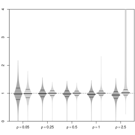
(b) $n=3$

Figure 4.1: Box-Percentile plots (Esty and Banfield, 2003) of estimated deletion rates $\hat{\rho}$ divided by true parameter $\rho$. The estimates are based on two-way comparisons (left boxes, darkgray) and the spacer frequency spectrum (right boxes, lightgray) for different deletion rates $\rho$. We use $\theta=100\rho$ in all cases. (a) Estimates based on a sample of size $n=2$; see Definition 4.1. (b) Estimates based on a sample of size $n=3$; see Definition 4.3

As Figure 4.1 shows, both estimation procedures give accurate results (in the sense that the estimator $\hat{\rho}$ is close to $\rho$, or $\hat{\rho}/\rho\approx 1$ in many cases), but there are some differences. Since the equal spacer likelihood methods are based on extensions of geometric distributions, the resulting estimators are (slightly) biased. In contrast, the likelihood based on the spacer frequency spectrum can be calculated from independent Poisson random variables (Baumdicker et al., 2010) and the corresponding estimator is thus unbiased. Concerning the variance of the estimators, the equal spacer likelihood methods give a slightly larger variance of the estimators for small $\rho$ (for $n=2,\rho\leq 0.25$, Fig. 4.1(a); and for $n=3,\rho\leq 0.5$, Fig. 4.1(b)). This might be due to the fact that this estimation procedure only takes spacers after the first common spacer into account. However, after the first equal spacer, most spacers are equal for low $\rho$, such that there is less signal in the data, making estimation of $\rho$ more difficult. Note that for larger loss rates (for $n=2,\rho\geq 0.5$, Fig. 4.1(a); and for $n=3,\rho\geq 1$, Fig. 4.1(b)), the estimate from panicmage has a much higher variance. This might be due to the fact that panicmage cannot estimate $\theta$ and $\rho$ separately and the likelihood surface is flat in one direction in the $\theta/\rho$-plane.

5 Discussion

The ordered independent loss model for CRISPR spacer evolution paves the way for various statistical applications based on equal spacers. However, when comparing the estimates for the spacer deletion rate with the unordered model in small sample sizes and limited deletion rates, the extra information of the order of spacers does not seem to produce more reliable results; see Figure 4.1. Nevertheless, this extra information will prove to be useful in further applications. In particular, since spacers are ordered by time of their insertion in each array, we can see which spacers in the arrays were present in the nodes of the phylogeny. If a spacer is present in a specific node in the phylogeny, all subsequent spacers were inserted before and hence must also be present within this node. This information is only available in the ordered model and will help to understand phenomena such as non-constant insertion rates or horizontal transfer.

The ordered independent loss model, as presented above, assumes constant insertion and deletion rates. The separate estimation of spacer insertion and deletion rates allows to investigate each mechanism independently. Besides selective effects, the insertion of spacers is more strongly dependent on the environment of the population than the random deletion of spacers is. The insertion might hence be time-dependent (Hynes et al., 2016b). In contrast, it is more reasonable to assume that the deletion of a neutral spacer occurs at constant rate. To test this hypothesis in future statistical work, we therefore aim at methods based on equal spacer distances. This will allow us to infer deletion rate variation between different branches in the given phylogeny, different CRISPR-Cas systems or positions in the spacer array.

To apply the presented approach to genmic data, the CRISPR spacer arrays and a reconstructed phylogeny are necessary. In addition the equal spacers among all the CRISPR arrays need to be identified. There are several CRISPR prediction tools that can be used to scan for spacer arrays in genomic data (Bland et al., 2007; Edgar, 2007; Grissa et al., 2007a). For archaeal and bacterial reference genomes predicted spacers are available online (Grissa et al., 2007b). While a typical array has less than 20 spacers, there are also arrays with several hundred spacers.

The ordered independent loss model will be useful to study the evolutionary ecology of CRISPR-Cas systems. For an extensive review of the evolution and ecology of CRISPR we refer the reader to Westra et al. (2016). Here we will highlight the role of spacer deletions in CRISPR-enhanced gene drives and metagenomic studies concerning CRISPR. Gene drive is the dependency of the offspring distribution of an individual on its genetic background. As such, this concept in concert with CRISPR can be used for the artificial alterations of natural populations (Burt, 2003; Hynes et al., 2016b). However, Unckless et al. (2017) argue that in natural populations resistance to a gene drive will likely occur. As a counter measure, different improvements of the CRISPR gene drive have been proposed (Esvelt et al., 2014). One suggestion is to use a CRISPR gene drive with more than one spacer, such that resistance can not evolve so easily. The effect of losing spacers in such a gene drive should be considered carefully before using any designed CRISPR system in natural populations. The same is true for the idea to ”vaccinate” bacteria possessing CRISPR via defective phage and plasmid sequences (Hynes et al., 2014, 2016a). Since any artificial CRISPR spacer insertion is transmitted to the offspring we should assess the fixation probabilities and extinction times of vaccinated bacterial strains before releasing them into natural environments.

To better understand the dynamics of CRISPR and the corresponding phages in natural populations metagenomic studies have been used. Using the sequenced CRISPR spacer arrays, the ancestral environment of the population can be inferred (Sun et al., 2015). In addition, different lineages can be distinguished, even for highly related bacterial strains (Kunin et al., 2008). Since the ordered independent loss model is based on a genealogical tree connecting the individuals, it cannot directly be used for metagenomic data. Nonetheless, the model provides a theoretical framework to have a more detailed look at the evolutionary pattern in the spacer array. In particular, the often observed conservation of old spacers at the trailer-end of the array is of interest (Weinberger et al., 2012). In the ordered independent loss model conservation of spacers correspond to small equal spacer distances, i.e. a low spacer deletion rate $\rho$. For large loss rates the number of spacers between equal spacers rises until finally all observed spacers differ. In a non-neutral setting with selection simulations of CRISPR arrays and the viral population show that the distances between equal spacers still increase for high spacer deletion rates. To which amount the CRISPR trailer-end is conserved due to selective forces compared to the effect of a low deletion rate remains a future challenge.

Acknowledgments

We thank Omer Alkhnbashi and Rolf Backofen for fruitful discussion and two anonymous referees for their constructive comments and hints. We thank an anonymous referee to encourage us to give our most general result, Theorem 3. This research was supported by the DFG through the priority program SPP1590. In particular, FB is funded in parts through Pf672/9-1.

Bibliography

Bibliography

• Barrangou et al. (2007) Barrangou, R., Fremaux, C., Deveau, H., Richards, M., Boyaval, P., Moineau, S., Romero, D.A., Horvath, P., 2007. CRISPR provides acquired resistance against viruses in prokaryotes. Science 315, 1709–1712.
• Baumdicker et al. (2010) Baumdicker, F., Hess, W., Pfaffelhuber, P., 2010. The diversity of a distributed genome in bacterial populations. The Annals of Applied Probability 20, 1567–1606.
• Baumdicker et al. (2012) Baumdicker, F., Pfaffelhuber, P., Hess, W., 2012. The infinitely many genes model for the distributed genome of bacteria. Genome Biology and Evolution 4, 443–456.
• Benjamini and Peres (1994) Benjamini, I., Peres, Y., 1994. Markov chains indexed by trees. The Annals of Probability 22, 219–243.
• Bland et al. (2007) Bland, C., Ramsey, T.L., Sabree, F., Lowe, M., Brown, K., Kyrpides, N.C., Hugenholtz, P., 2007. CRISPR Recognition Tool (CRT): a tool for automatic detection of clustered regularly interspaced palindromic repeats. BMC Bioinformatics 8, 209.
• Bolotin et al. (2005) Bolotin, A., Quinquis, B., Sorokin, A., Dusko Ehrlich, S., 2005. Clustered regularly interspaced short palindrome repeats (CRISPRs) have spacers of extrachromosomal origin. Microbiology 151, 2551–2561.
• Burt (2003) Burt, A., 2003. Site-specific selfish genes as tools for the control and genetic engineering of natural populations. Proceedings of the Biological Sciences B 270, 921–928.
• Childs et al. (2014) Childs, L.M., England, W.E., Young, M.J., Weitz, J.S., Whitaker, R.J., 2014. Crispr-induced distributed immunity in microbial populations. PloS one 9, e101710.
• Doudna and Charpentier (2014) Doudna, J.A., Charpentier, E., 2014. The new frontier of genome engineering with crispr-cas9. Science 346.
• Edgar (2007) Edgar, R.C., 2007. PILER-CR: fast and accurate identification of CRISPR repeats. BMC Bioinformatics 8, 1–6.
• Esty and Banfield (2003) Esty, W.W., Banfield, J.D., 2003. The Box-Percentile Plot. Journal of Statistical Software 8, 1–14.
• Esvelt et al. (2014) Esvelt, K.M., Smidler, A.L., Catteruccia, F., Church, G.M., 2014. Concerning RNA-guided gene drives for the alteration of wild populations. eLife 3, e03401.
• Grissa et al. (2007a) Grissa, I., Vergnaud, G., Pourcel, C., 2007a. CRISPRFinder: a web tool to identify clustered regularly interspaced short palindromic repeats. Nucleic Acids Research 35, W52–W57.
• Grissa et al. (2007b) Grissa, I., Vergnaud, G., Pourcel, C., 2007b. The CRISPRdb database and tools to display CRISPRs and to generate dictionaries of spacers and repeats. BMC Bioinformatics 8, 172.
• Han and Deem (2017) Han, P., Deem, M.W., 2017. Non-classical phase diagram for virus bacterial coevolution mediated by clustered regularly interspaced short palindromic repeats. Journal of The Royal Society Interface 14.
• Horvath et al. (2008) Horvath, P., Romero, D.A., Coûté-Monvoisin, A.C., Richards, M., Deveau, H., Moineau, S., Boyaval, P., Fremaux, C., Barrangou, R., 2008. Diversity, activity, and evolution of CRISPR loci in Streptococcus thermophilus. Journal of Bacteriology 190, 1401–1412.
• Hsu et al. (2014) Hsu, P., Lander, E., Zhang, F., 2014. Development and Applications of CRISPR-Cas9 for Genome Engineering. Cell 157, 1262–1278.
• Hynes et al. (2016a) Hynes, A.P., Labrie, S.J., Moineau, S., 2016a. Programming Native CRISPR Arrays for the Generation of Targeted Immunity. mBio 7, e00202–16.
• Hynes et al. (2016b) Hynes, A.P., Lemay, M.L., Moineau, S., 2016b. Applications of CRISPR-Cas in its natural habitat. Current Opinion in Chemical Biology 34, 30–36.
• Hynes et al. (2014) Hynes, A.P., Villion, M., Moineau, S., 2014. Adaptation in bacterial CRISPR-Cas immunity can be driven by defective phages. Nature Communications 5, 1–6.
• Ishino et al. (1987) Ishino, Y., Shinagawa, H., Makino, K., Amemura, M., Nakata, A., 1987. Nucleotide sequence of the iap gene, responsible for alkaline phosphatase isozyme conversion in Escherichia coli, and identification of the gene product. Journal of Bacteriology 169, 5429–5433.
• Koonin and Wolf (2016) Koonin, E.V., Wolf, Y.I., 2016. Just how Lamarckian is CRISPR-Cas immunity: the continuum of evolvability mechanisms. Biology Direct 11, 9.
• Koskella and Brockhurst (2014) Koskella, B., Brockhurst, M.A., 2014. Bacteria-phage coevolution as a driver of ecological and evolutionary processes in microbial communities. FEMS Microbiology Reviews 38, 916–931.
• Kunin et al. (2008) Kunin, V., He, S., Warnecke, F., Peterson, S.B., Garcia Martin, H., Haynes, M., Ivanova, N., Blackall, L.L., Breitbart, M., Rohwer, F., McMahon, K.D., Hugenholtz, P., 2008. A bacterial metapopulation adapts locally to phage predation despite global dispersal. Genome Research 18, 293–7.
• Kupczok and Bollback (2013) Kupczok, A., Bollback, J.P., 2013. Probabilistic models for CRISPR spacer content evolution. BMC Evolutionary Biology 13, 54.
• Kupczok et al. (2015) Kupczok, A., Landan, G., Dagan, T., 2015. The contribution of genetic recombination to CRISPR array evolution. Genome Biology and Evolution 7, 1925–1939.
• Levin (2010) Levin, B.R., 2010. Nasty viruses, costly plasmids, population dynamics, and the conditions for establishing and maintaining crispr-mediated adaptive immunity in bacteria. PLoS genetics 6, e1001171.
• Lopez-Sanchez et al. (2012) Lopez-Sanchez, M.J., Sauvage, E., Da Cunha, V., Clermont, D., Ratsima Hariniaina, E., Gonzalez-Zorn, B., Poyart, C., Rosinski-Chupin, I., Glaser, P., 2012. The highly dynamic CRISPR1 system of Streptococcus agalactiae controls the diversity of its mobilome. Molecular Microbiology 85, 1057–1071.
• Makarova et al. (2011a) Makarova, K.S., Aravind, L., Wolf, Y.I., Koonin, E.V., 2011a. Unification of cas protein families and a simple scenario for the origin and evolution of crispr-cas systems. Biology Direct 6, 38.
• Makarova et al. (2011b) Makarova, K.S., Haft, D.H., Barrangou, R., Brouns, S.J.J., Charpentier, E., Horvath, P., Moineau, S., Mojica, F.J.M., Wolf, Y.I., Yakunin, A.F., van der Oost, J., Koonin, E.V., 2011b. Evolution and classification of the CRISPR–Cas systems. Nature Reviews Microbiology 9, 467–477.
• Makarova et al. (2015) Makarova, K.S., Wolf, Y.I., Alkhnbashi, O.S., Costa, F., Shah, S.A., Saunders, S.J., Barrangou, R., Brouns, S.J.J., Charpentier, E., Haft, D.H., Horvath, P., Moineau, S., Mojica, F.J.M., Terns, R.M., Terns, M.P., White, M.F., Yakunin, A.F., Garrett, R.A., van der Oost, J., Backofen, R., Koonin, E.V., 2015. An updated evolutionary classification of CRISPR-Cas systems. Nature Reviews Microbiology 13, 722–736.
• Marraffini (2015) Marraffini, L.A., 2015. CRISPR-Cas immunity in prokaryotes. Nature 526, 55–61.
• Mira et al. (2010) Mira, A., Martín-Cuadrado, A.B., D’Auria, G., Rodríguez-Valera, F., 2010. The bacterial pan-genome: a new paradigm in microbiology. International Microbiology: The Official Journal of the Spanish Society for Microbiology 13, 45–57.
• Oye et al. (2014) Oye, K.A., Esvelt, K., Appleton, E., Catteruccia, F., Church, G., Kuiken, T., Lightfoot, S.B.Y., McNamara, J., Smidler, A., Collins, J.P., 2014. Regulating gene drives. Science 345.
• Rath et al. (2015) Rath, D., Amlinger, L., Rath, A., Lundgren, M., 2015. The CRISPR-Cas immune system: Biology, mechanisms and applications. Biochimie 117, 119–128.
• Sun et al. (2015) Sun, C.L., Thomas, B.C., Barrangou, R., Banfield, J.F., 2015. Metagenomic reconstructions of bacterial CRISPR loci constrain population histories. The ISME Journal 10, 1–13.
• Unckless et al. (2017) Unckless, R.L., Clark, A.G., Messer, P.W., 2017. Evolution of Resistance Against CRISPR/Cas9 Gene Drive. Genetics 205.
• Vernikos et al. (2014) Vernikos, G., Medini, D., Riley, D.R., Tettelin, H., 2014. Ten years of pan-genome analyses. Current Opinion in Microbiology 23C, 148–154.
• Wakeley (2008) Wakeley, J., 2008. Coalescent Theory: An Introduction. Roberts & Company.
• Weinberger et al. (2012) Weinberger, A.D., Wolf, Y.I., Lobkovsky, A.E., Gilmore, M.S., Koonin, E.V., 2012. Viral diversity threshold for adaptive immunity in prokaryotes. mBio 3, e00456–12.
• Westra et al. (2014) Westra, E.R., Buckling, A., Fineran, P.C., 2014. CRISPR–Cas systems: beyond adaptive immunity. Nature Reviews Microbiology 12, 317–326.
• Westra et al. (2016) Westra, E.R., Dowling, A.J., Broniewski, J.M., van Houte, S., 2016. Evolution and Ecology of CRISPR. Annual Review of Ecology, Evolution, and Systematics 47, 307–331.