Thermal and nonthermal scaling of the Casimir-Polder interaction
in a black hole spacetime

Abstract

We study the Casimir-Polder force arising between two identical two-level atoms and mediated by a massless scalar field propagating in a black-hole background. We study the interplay of Hawking radiation and Casimir-Polder forces and find that, when the atoms are placed near the event horizon, the scaling of the Casimir-Polder interaction energy as a function of interatomic distance displays a transition from a thermallike character to a nonthermal behavior. We corroborate our findings for a quantum field prepared in the Boulware, Hartle-Hawking, and Unruh vacua. Our analysis is consistent with the nonthermal character of the Casimir-Polder interaction of two-level atoms in a relativistic accelerated frame [J. Marino et al., Phys. Rev. Lett. 113, 020403 (2014)], where a crossover from thermal scaling, consistent with the Unruh effect, to a nonthermal scaling has been observed. The two crossovers are a consequence of the noninertial character of the background where the field mediating the Casimir interaction propagates. While in the former case the characteristic crossover length scale is proportional to the inverse of the surface gravity of the black hole, in the latter it is determined by the inverse of the proper acceleration of the atoms.

I Introduction

The relationship between quantum theory and the gravitational field is a very special one oup . While standard quantum (field) theory is formulated on a fixed background, gravity is described by a dynamical spacetime. This difference is the major obstacle for a consistent quantization.

Black holes are assumed to play a key role in the search for a quantum theory of gravity. This is because they obey laws which are closely analogous to the laws of thermodynamics. The interpretation of these laws necessarily invokes quantum theory because classically a black hole cannot radiate and thus cannot be attributed a temperature. Using the formalism of quantum field theory on a classical dynamical spacetime (see e.g. birrel ; frolov ), Hawking has shown that black holes radiate with a temperature proportional to $\hbar$, which in the case of a Schwarzschild black hole is given by $T=\hbar c^{3}/8\pi k_{\rm B}GM$ hawking .

The interpretation and consequences of this temperature are still subject of investigations; see, for example, Jerusalem for a recent review. If this radiation were exactly thermal and if the black hole evaporated completely, any initial (quantum) state would evolve into the same final thermal state, in violation of the unitary time evolution of ordinary quantum theory. This “information-loss problem” can eventually only be solved within a final theory of quantum gravity.

Besides particle creation, an important effect in black-hole spacetimes is vacuum polarization frolov . A similar effect in flat spacetime occurs in the presence of nontrivial boundaries – the Casimir effect casimir ; plunien ; grib ; bordag ; book ; Milonni . The physical reality of this effect has been empirically confirmed in a variety of experiments L07 . In its classic formulation, the Casimir effect is the attraction of two neutral conducting plates at zero temperature as a result of a quantum pressure induced by vacuum fluctuations. Even before, Casimir and Polder have investigated the attraction between an atom and a perfectly conducting wall as well as between two atoms CP48 . Both Casimir and Casimir-Polder forces have been explored in the presence of boundary conditions and nontrivial backgrounds which can modify the quantization conditions of the field modes and accordingly the structure of correlations in the quantum vacuum. See also Ref. farina for a recent study of the Casimir-Polder interaction in graphene.

In this paper, we address the Casimir-Polder interaction between two atoms. When embedded in a quantum vacuum, they experience a force as a result of local dipoles spontaneously induced on them by correlated zero-point vacuum fluctuations. We consider this interaction in a black-hole spacetime and thus present a situation in which the quantum aspects of black holes and the quantum aspects of the standard Casimir-Polder force are intertwined. In this respect, we also remark the existence of a number of previous studies on the gravitation interaction of the Casimir energy milton .

A useful technique, widely employed in the literature, is a method developed by Dalibard, Dupont-Roc, and Cohen-Tannoudji (DDC) in order to separate in perturbation theory the distinct contributions of vacuum fluctuations and radiation reaction to radiative shifts of atomic energy levels cohen2 . The method was originally formulated to treat a small system coupled to a reservoir cohen3 ; in this case, it was shown that two types of physical processes contribute to the evolution of an observable, those where the fluctuation of the reservoir polarizes the system and those where it is the system itself that polarizes the reservoir. If the system is a quantized field, we call the former vacuum fluctuations and the latter radiation reaction contributions.

In second order perturbation theory, the aforementioned method has been successfully applied to computing space-dependent radiative shifts of atoms in front of a reflecting plate – also known as atom-plate Casimir force Rizzuto . Moreover, it has also been employed to investigate the radiative processes of entangled atoms in Minkowski spacetime ng1 and also in the presence of an event horizon ng2 ; ng3 .

However, only recently the method by DDC has been extended to fourth order in perturbation theory for atoms linearly coupled to a scalar field marino ; noto , as necessary to compute the Casimir-Polder force between two polarizable, neutral atoms in their respective ground states.

Outline of results

(i) Casimir-Polder interaction in a black-hole spacetime – We examine the Casimir-Polder interaction between two identical two-level atoms in a Schwarzschild spacetime, linearly coupled with the quantum fluctuations of a scalar field prepared in the Boulware, Hartle-Hawking, and Unruh vacuum states. Similar computations have already been performed with a different atomic configuration, considering an electromagnetic field and employing the method of equal-time spatial vacuum field fluctuations bh . In this paper, we explore a broader variety of parameters, considering the interplay of the interatomic distance, energy level spacing of the atoms, and the surface gravity of the black hole. In particular, we highlight the regimes where the Casimir-Polder force exhibits a nonthermal scaling with the interatomic distance; indeed, while for certain choices of parameters, the Casimir interaction displays a thermal character linked to its Hawking temperature, at large enough interatomic separations, and close to the black-hole horizon, the noninertial character of the background metric modifies the scaling of the force in a nonthermal fashion.

We derive these results calculating the vacuum fluctuation and radiation reaction contributions to the Casimir-Polder interaction at fourth order in perturbation theory in the atom-field coupling strength (see for a derivation  noto ). The vacuum fluctuation term can be interpreted as the fluctuations of the zero-point field inducing local dipoles on the atoms, which leads to a coupling between the atoms, while the radiation reaction term reflects the opposite mechanism: when one of the atom experiences quantum fluctuations, it polarizes the remainder of the system (the field and the other atom). The associated expressions for the radiative energy level shifts (Eqs. (3-4) below and Refs. marino ; noto ) provide a set of general formulae to compute Casimir-Polder forces from first principles without resorting to specific phenomenological models.

(ii) Analogy with the Casimir-Polder interaction of two relativistic uniformly accelerated atoms – We discuss the analogy with a similar phenomenology encountered in Ref. marino (also notice similar studies in rizzutoUnruh ), where the large-distance scaling of the Casimir interaction among two relativistic uniformly accelerated atoms was studied. Close to the event horizon, the Schwarzschild metric takes the form of the Rindler line element, and we find that the characteristic exponent of the algebraic scaling discussed in marino is perfectly mirrored in the large interatomic separation scaling of the Casimir force close to the black hole. The nonthermal correction to the Casimir interaction is imprinted by the noninertial character of the background metric which becomes sizeable at distances larger than the inverse of the surface gravity of the black hole, that is, larger than $4GM/c^{2}$.

The organization of the paper is as follows. In Sec. II, we setup our system and discuss the identification of vacuum fluctuations and radiation reaction corrections at fourth order in perturbation theory to the radiative energy shifts of the atoms. In Sec. III, we calculate the Casimir-Polder interaction energy for static atoms outside a Schwarzschild black hole and compare it with analogous results for relativistically uniformly accelerated atoms marino . Conclusions and final remarks are given in Sec. IV. In the Appendix, we present the correlation functions for a scalar field in Schwarzschild spacetime.

In this paper, we use units such that $\hbar=c=k_{B}=1$, but include some remarks on the dependence of the results on such constants. We employ the convention that the Minkowski signature is given by $\eta_{\alpha\beta}=-1,\alpha=\beta=1,2,3$, $\eta_{\alpha\beta}=1,\alpha=\beta=0$ and $\eta_{\alpha\beta}=0,\alpha\neq\beta$.

II The model and the method

In the following, we consider two identical two-level atoms interacting with a quantum massless scalar field. The atoms move along different world lines in a four-dimensional Schwarzschild spacetime,

$$ds^{2}=g_{00}dt^{2}-{g^{-1}_{00}}dr^{2}-r^{2}(d\theta^{2}+\sin^{2}\theta d\phi^{2}),$$ (1)

where $g_{00}=\left(1-r_{s}/r\right)$ and $r_{s}=2GM$ is the Schwarzschild radius. Eq. (1) describes the gravitational field outside a spherically symmetric body of mass $M$ in spherical coordinates $(r,\theta,\phi)$. The collapse of an electrically neutral, static star endowed with spherical symmetry produces a spherical black hole of mass $M$ with external gravitational field, described by the Schwarzschild line element (1), and with the event horizon of the black hole being located at the Schwarzschild radius $r_{s}$.

Our goal is to compute the Casimir-Polder force between the two atoms mediated by a massless scalar field propagating in a spacetime described by the metric (1). We employ a general method for the computation of Casimir-Polder interaction energy from first principles. The approach we use is the DDC formalism up to fourth order in perturbation theory, following closely Refs. marino ; noto . In particular, we consider the contribution to the interaction energy coming from the interplay between vacuum fluctuations and radiation reaction among the two identical two-level atoms linearly coupled with the scalar field. We assume that both atoms are moving along different stationary trajectories $x^{\mu}(\tau_{i})=(t(\tau_{i}),{\bf x}(\tau_{i}))$, where $\tau_{i}$ denotes the proper time of atom $i$ ($i=A,B$). The Hamiltonian of the system reads Rizzuto

$$H(t) = \omega_{0}\,\sigma_{3}^{A}\,\frac{d\tau_{A}}{dt}+\omega_{0}\,\sigma_{3}^{B}\,\frac{d\tau_{B}}{dt}+\sum_{{\bf k}}\,\omega_{{\bf k}}\,a^{\dagger}_{{\bf k}}(t)a_{{\bf k}}(t)$$ (2)

$$+ \lambda\sigma_{2}^{A}\,\varphi(x_{A}(\tau_{A}))\,\frac{d\tau_{A}}{dt}+\lambda\sigma_{2}^{B}\,\varphi(x_{B}(\tau_{B}))\,\frac{d\tau_{B}}{dt},$$

where $d\tau/dt=\sqrt{g_{00}}$, and $t$ is the Schwarzschild coordinate time. In Eq. (2), $\sigma_{3}^{j}=1/2\left(|e_{j}\rangle\langle e_{j}|-|g_{j}\rangle\langle g_{j}|\right)$, $j=A,B$, $\omega_{{\bf k}}=|{\bf k}|$, $a^{\dagger}_{{\bf k}},a_{{\bf k}}$ are the usual creation and annihilation operators of the scalar field quanta with momentum $\bf k$. The states $|g_{A}\rangle$, $|g_{B}\rangle$ and $|e_{A}\rangle$, $|e_{B}\rangle$ denote the ground and excited states of isolated atoms with energies $-\omega_{0}/2$ and $\omega_{0}/2$, respectively. One can write $\sigma_{2}^{j}=(i/2)(\sigma_{-}^{j}-\sigma_{+}^{j})$, $j=A,B$, where $\sigma_{\pm}^{j}$ are the usual atomic raising and lowering operators, satisfying the algebra: $[\sigma_{3}^{i},\sigma_{\pm}^{j}]=\pm\sigma_{\pm}^{i}\delta^{ij}$ and $[\sigma_{+}^{i},\sigma_{-}^{j}]=2\sigma_{3}^{i}\delta^{ij}$. Finally, $\lambda$ is the light-matter coupling strength.

A brief comment on the units employed in this work is in order. Here the field $\varphi$ has the usual mass dimension, while $\lambda$ is dimensionless. If we reinsert $\hbar$, $\varphi^{2}$ has dimension of mass over length, while $\lambda^{2}$ has dimension of mass times length.

The DDC approach allows us to identify two different contributions in the expectation value of a given atomic observable cohen2 ; cohen3 ; the first is generally refered to as vacuum fluctuation (vf) term and it accounts for the response of the atom to zero-point quantum fluctuations of the field, while the other term accounts for the backreaction on the atom, as a result of its interaction with the field – it is the radiation reaction (rr). Here, we do not give a detailed treatment of the DDC formalism, since it has been discussed to full extent in the papers cited above; we will directly present, instead, the final outcome of the derivation of a fourth-order perturbative computation ($\lambda$ is the small parameter) of the vf and rr contributions to the radiative correction of the atomic bare energy, $\omega_{0}$, of a given atom marino ; noto . In particular, in order to extract the Casimir-Polder interaction, the part of energy shift of interest is the contribution at fourth order in the atom-field interaction that depends on the interatomic distance (since the other fourth-order terms are just renormalizations of the bare energy $\omega_{0}$).

We focus, for instance, on the radiative shift to the level $|\alpha\rangle$ of atom $A$, and we take the average of field operators in the vacuum state of the quantum field $|0\rangle$ as well as the expectation value of atomic operators in the state $|\nu\rangle$ of atom $B$. After a lengthy algebra, we find the following expression for the vacuum-fluctuation and radiation-reaction contributions to the energy level shift of atom $A$ in the state $|\alpha\rangle$:

$$(\delta E)^{A}_{\alpha,\textrm{vf}} = \frac{i\lambda^{4}}{4}\,\int_{t_{0}}^{t}dt^{\prime}\,\int_{t_{0}}^{t^{\prime}}dt^{\prime\prime}\,\int_{t_{0}}^{t^{\prime\prime}}dt^{\prime\prime\prime}\,D[x_{A}(\tau_{A}(t)),x_{B}(\tau_{B}^{\prime\prime\prime}(t^{\prime\prime\prime})))]\Delta[x_{A}(\tau_{A}^{\prime}(t^{\prime})),x_{B}(\tau_{B}^{\prime\prime}(t^{\prime\prime})))]\,$$ (3)

$$\times \,\chi^{A}_{\alpha}[\tau_{A}(t),\tau_{A}^{\prime}(t^{\prime})]\,\chi^{B}_{\beta}[\tau_{B}^{\prime\prime}(t^{\prime\prime}),\tau_{B}^{\prime\prime\prime}(t^{\prime\prime\prime})]\frac{d\tau_{A}}{dt}\frac{d\tau_{A}^{\prime}}{dt^{\prime}}\frac{d\tau_{B}^{\prime\prime}}{dt^{\prime\prime}}\frac{d\tau_{B}^{\prime\prime\prime}}{dt^{\prime\prime\prime}}$$

and

$$(\delta E)^{A}_{\alpha,\textrm{rr}} = -\frac{i\lambda^{4}}{4}\,\int_{t_{0}}^{t}dt^{\prime}\,\int_{t_{0}}^{t^{\prime}}dt^{\prime\prime}\,\int_{t_{0}}^{t^{\prime\prime}}dt^{\prime\prime\prime}\,\Delta[x_{A}(\tau_{A}(t)),x_{B}(\tau_{B}^{\prime}(t^{\prime})))]\Delta[x_{A}(\tau_{A}^{\prime\prime\prime}(t^{\prime\prime\prime})),x_{B}(\tau_{B}^{\prime\prime}(t^{\prime\prime})))]\,$$ (4)

$$\times \,C^{A}_{\alpha}[\tau_{A}(t),\tau_{A}^{\prime\prime\prime}(t^{\prime\prime\prime})]\,\chi^{B}_{\beta}[\tau_{B}^{\prime}(t^{\prime}),\tau_{B}^{\prime\prime}(t^{\prime\prime})]\frac{d\tau_{A}}{dt}\frac{d\tau_{B}^{\prime}}{dt^{\prime}}\frac{d\tau_{B}^{\prime\prime}}{dt^{\prime\prime}}\frac{d\tau_{A}^{\prime\prime\prime}}{dt^{\prime\prime\prime}}.$$

In all equations above, we make use of the following definitions:

$$\chi^{kl}_{\nu}(t,t^{\prime}):=\langle\nu|[\sigma_{2}^{k,f}(\tau_{k}(t)),\sigma_{2}^{l,f}(\tau_{l}(t^{\prime}))]|\nu\rangle,$$ (5)

($\chi^{kk}_{\nu}\equiv\chi^{k}_{\nu}$) $k,l=A,B$, is the atomic susceptibility of the atom in the state $|\nu\rangle$, and

$$C^{kl}_{\nu}(t,t^{\prime}):=\langle\nu|[\sigma_{2}^{k,f}(\tau_{k}(t)),\sigma_{2}^{l,f}(\tau_{l}(t^{\prime}))]|\nu\rangle,$$ (6)

($C^{kk}_{\nu}\equiv C^{k}_{\nu}$) is the symmetric correlation function of the atom in the state $|\nu\rangle$. (The suffix $f$ indicates that we are in the interacton picture where we have the free evolution of the atomic observables.)

The explicit forms of these quantities are given by

$$\chi^{ab}_{\nu}(t,t^{\prime}) = \sum_{\nu^{\prime}}\biggl{[}{\cal A}^{ab}(\nu,\nu^{\prime})\,e^{i\Delta\nu(\tau_{a}(t)-\tau_{b}^{\prime}(t^{\prime}))}$$ (7)

$$- \,{\cal A}^{ba}(\nu,\nu^{\prime})\,e^{-i\Delta\nu(\tau_{a}(t)-\tau_{b}^{\prime}(t^{\prime}))}\biggr{]},$$

and

$$C^{ab}_{\nu}(t,t^{\prime}) = \sum_{\nu^{\prime}}\biggl{[}{\cal A}^{ab}(\nu,\nu^{\prime})\,e^{i\Delta\nu(\tau_{a}(t)-\tau_{b}^{\prime}(t^{\prime}))}$$ (8)

$$+ \,{\cal A}^{ba}(\nu,\nu^{\prime})\,e^{-i\Delta\nu(\tau_{a}(t)-\tau_{b}^{\prime}(t^{\prime}))}\biggr{]},$$

where $\Delta\nu:=\omega_{0}(\nu-\nu^{\prime})$ (the summation over $\nu^{\prime}$ is over the product state basis or, in the case of one atom, over $|g\rangle,|e\rangle$), and we have conveniently introduced the function ${\cal A}_{ab}^{ij}(\nu,\nu^{\prime})$ defined as

$${\cal A}^{ab}(\nu,\nu^{\prime})=\langle\nu|\sigma_{2}^{a,f}(0)|\nu^{\prime}\rangle\langle\nu^{\prime}|\sigma_{2}^{b,f}(0)|\nu\rangle.$$ (9)

For the field variables, one has

$$D(x(\tau),x(\tau^{\prime}))=\langle 0|\{\varphi^{f}(x(\tau)),\varphi^{f}(x(\tau^{\prime}))\}|0\rangle,$$ (10)

which is the symmetric correlation function of the scalar field (also known as Hadamard’s elementary function) and

$$\Delta(x(\tau),x(\tau^{\prime}))=\langle 0|[\varphi^{f}(x(\tau)),\varphi^{f}(x(\tau^{\prime}))]|0\rangle,$$ (11)

which is the response function of the field (or Pauli-Jordan function).

The physical interpretation of Eqs. (3) and (4) can be read from the type of response or correlation functions entering these expressions. Regarding $\delta E_{vf}$, the field fluctuates around the two atoms $A$ and $B$ ($D_{AB}$), and they respond with a local polarization $\chi^{A}$ and $\chi^{B}$, which results in the transmission of a quantum of the field between them (response field, $\Delta_{AB}$), or in other words, the medium among them gets polarized. Regarding $\delta E_{rr}$, the atom $A$ fluctuates ($C^{A}$), and polarizes the remaining components of the system: the atom $B$ ($\chi^{B}$) and the field ($\Delta_{AB}$).

III Casimir-Polder interaction

We consider the two atoms prepared in their respective ground states, static and at fixed Schwarzschild radial coordinates $r_{A}$ and $r_{B}$ outside the black hole. The world lines are given respectively by $x^{\mu}(\tau_{i})=(\tau_{i}/\sqrt{g_{00(r_{i})}},r_{i},\theta_{i},\phi_{i})$, $i=A,B$, and $g_{00}(r)=1-2GM/r$ (the angular coordinates $\theta_{i},\phi_{i}$ are constants). In order to employ the formulae (3) and (4), one should use the associated correlation functions of the scalar field. The correlation functions of a massless scalar field in Schwarzschild spacetime for each one of the possible vacua (Boulware, Hartle-Hawking, Unruh) discussed in the literature is briefly outlined in the Appendix (where we present the computation of the correlations functions relevant to extract $\Delta$ and $D$). For further details, we refer to Ref. frolov .

III.1 Boulware vacuum

The Boulware vacuum has a close similarity to the concept of an empty state at large radii. It is the appropriate choice of vacuum state for quantum fields in the vicinity of an isolated, cold neutron star; the Boulware vacuum is relevant to the exterior region of a massive body that is just outside its Schwarzschild radius boul ; sciama .

The associated symmetric correlation function is given by

$$D^{B}(x_{i}(t),x_{j}(t^{\prime})) = \frac{1}{16\pi^{2}}\sum_{l=0}^{\infty}(2l+1)P_{l}(\hat{r}_{i}\cdot\hat{r}_{j})\int_{0}^{\infty}\,\frac{d\omega}{\omega}\,\Biggl{\{}e^{-i\omega(t-t^{\prime})}\left[\overrightarrow{R}_{\omega l}(r_{i})\overrightarrow{R}^{*}_{\omega l}(r_{j})+\overleftarrow{R}_{\omega l}(r_{i})\overleftarrow{R}^{*}_{\omega l}(r_{j})\right]$$ (12)

$$+ \,e^{i\omega(t-t^{\prime})}\left[\overrightarrow{R}_{\omega l}(r_{j})\overrightarrow{R}^{*}_{\omega l}(r_{i})+\overleftarrow{R}_{\omega l}(r_{j})\overleftarrow{R}^{*}_{\omega l}(r_{i})\right]\Biggr{\}},$$

where the addition theorem for the spherical harmonics was used hilbert , $\hat{r}_{i}$ and $\hat{r}_{j}$ (with $i,j=A,B$) are two unit vectors with spherical coordinates $(\theta_{i},\phi_{i})$ and $(\theta_{j},\phi_{j})$, respectively, $P_{l}$ is the Legendre polynomial of degree $l$ abram and the radial functions $\overrightarrow{R}$ and $\overleftarrow{R}$ are introduced in the Appendix. The response function is given by

$$\Delta^{B}(x_{i}(t),x_{j}(t^{\prime})) = \frac{1}{16\pi^{2}}\sum_{l=0}^{\infty}(2l+1)P_{l}(\hat{r}_{i}\cdot\hat{r}_{j})\int_{0}^{\infty}\,\frac{d\omega}{\omega}\,\Biggl{\{}e^{-i\omega(t-t^{\prime})}\left[\overrightarrow{R}_{\omega l}(r_{i})\overrightarrow{R}^{*}_{\omega l}(r_{j})+\overleftarrow{R}_{\omega l}(r_{i})\overleftarrow{R}^{*}_{\omega l}(r_{j})\right]$$ (13)

$$- e^{i\omega(t-t^{\prime})}\left[\overrightarrow{R}_{\omega l}(r_{j})\overrightarrow{R}^{*}_{\omega l}(r_{i})+\overleftarrow{R}_{\omega l}(r_{j})\overleftarrow{R}^{*}_{\omega l}(r_{i})\right]\Biggr{\}}.$$

In this way, using ${\cal A}^{AA}(\nu,\nu^{\prime})={\cal A}^{BB}(\nu,\nu^{\prime})=1/4$, with $|\nu\rangle=|g\rangle$ being the atomic ground state $|g\rangle$ (the only contribution in the summation over $\nu^{\prime}$ appearing in the atomic correlation functions comes from the excited state $|\nu^{\prime}\rangle=|e\rangle$), one has, for the vacuum fluctuation contribution

$$(\delta E)^{A}_{g,\textrm{vf}} = \frac{i\lambda^{4}}{2^{14}\pi^{4}}\,g_{00}(r_{A})g_{00}(r_{B})\int_{0}^{\infty}\,\frac{d\omega}{\omega}\int_{0}^{\infty}\,\frac{d\omega^{\prime}}{\omega^{\prime}}\int_{t_{0}}^{t}dt^{\prime}\,\int_{t_{0}}^{t^{\prime}}dt^{\prime\prime}\,\int_{t_{0}}^{t^{\prime\prime}}dt^{\prime\prime\prime}$$ (14)

$$\times \,\left[e^{-i\omega(t-t^{\prime\prime\prime})}B(\omega,r_{A},r_{B})+e^{i\omega(t-t^{\prime\prime\prime})}B(\omega,r_{B},r_{A})\right]$$

$$\times \,\left[e^{-i\omega^{\prime}(t^{\prime}-t^{\prime\prime})}B(\omega^{\prime},r_{A},r_{B})-e^{i\omega^{\prime}(t^{\prime}-t^{\prime\prime})}B(\omega^{\prime},r_{B},r_{A})\right]$$

$$\times \,\biggl{[}e^{i\omega_{A}(t-t^{\prime})}-e^{-i\omega_{A}(t-t^{\prime})}\biggr{]}\biggl{[}e^{i\omega_{B}(t^{\prime\prime}-t^{\prime\prime\prime})}-e^{-i\omega_{B}(t^{\prime\prime}-t^{\prime\prime\prime})}\biggr{]},$$

where $\omega_{A}=-\sqrt{g_{00}(r_{A})}\,\omega_{0}$, $\omega_{B}=-\sqrt{g_{00}(r_{B})}\,\omega_{0}$. The appearance of $\sqrt{g_{00}}$ multiplying the energy gap is a consequence of the usual gravitational redshift effect. In addition, we have defined $B(\omega,r,r^{\prime})=\overrightarrow{B}(\omega,r,r^{\prime})+\overleftarrow{B}(\omega,r,r^{\prime})$, with

$$\overrightarrow{B}(\omega,r,r^{\prime}) = \sum_{l=0}^{\infty}(2l+1)P_{l}(\hat{r}\cdot\hat{r}^{\prime})\overrightarrow{R}_{\omega l}(r)\overrightarrow{R}^{*}_{\omega l}(r^{\prime}),$$

$$\overleftarrow{B}(\omega,r,r^{\prime}) = \sum_{l=0}^{\infty}(2l+1)P_{l}(\hat{r}\cdot\hat{r}^{\prime})\overleftarrow{R}_{\omega l}(r)\overleftarrow{R}^{*}_{\omega l}(r^{\prime}).$$ (15)

Regarding the radiation reaction contribution, one gets

$$(\delta E)^{A}_{g,\textrm{rr}} = -\frac{i\lambda^{4}}{2^{14}\pi^{4}}\,g_{00}(r_{A})g_{00}(r_{B})\,\int_{0}^{\infty}\,\frac{d\omega}{\omega}\int_{0}^{\infty}\,\frac{d\omega^{\prime}}{\omega^{\prime}}\int_{t_{0}}^{t}dt^{\prime}\,\int_{t_{0}}^{t^{\prime}}dt^{\prime\prime}\,\int_{t_{0}}^{t^{\prime\prime}}dt^{\prime\prime\prime}$$ (16)

$$\times \,\left[e^{-i\omega(t-t^{\prime})}B(\omega,r_{A},r_{B})-e^{i\omega(t-t^{\prime})}B(\omega,r_{B},r_{A})\right]$$

$$\times \,\left[e^{-i\omega^{\prime}(t^{\prime\prime\prime}-t^{\prime\prime})}B(\omega^{\prime},r_{A},r_{B})-e^{i\omega^{\prime}(t^{\prime\prime\prime}-t^{\prime\prime})}B(\omega^{\prime},r_{B},r_{A})\right]$$

$$\times \,\biggl{[}e^{i\omega_{A}(t-t^{\prime\prime\prime})}+e^{-i\omega_{A}(t-t^{\prime\prime\prime})}\biggr{]}\biggl{[}e^{i\omega_{B}(t^{\prime}-t^{\prime\prime})}-e^{-i\omega_{B}(t^{\prime}-t^{\prime\prime})}\biggr{]}.$$

III.1.1 Atoms far from the black hole

In order to keep the discussion transparent, let us discuss the radiative energy shifts for the asymptotic regions of interest, keeping $|{\bf x}_{A}-{\bf x}_{B}|$ fixed. First, we consider the case $r_{A},r_{B}\to\infty$. Following the discussion presented in the Appendix, one can neglect the contribution coming from $\overrightarrow{B}$. For $\overleftarrow{B}$, we get

$$\overleftarrow{B}(\omega,r,r^{\prime}) = \sum_{l=0}^{\infty}(2l+1)\,P_{l}(\hat{r}\cdot\hat{r}^{\prime})\overleftarrow{R}_{\omega l}(r)\overleftarrow{R}^{*}_{\omega l}(r^{\prime})\approx\,4\omega\,\frac{\sin\left(\omega|{\bf x}-{\bf x}^{\prime}|\right)}{|{\bf x}-{\bf x}^{\prime}|},\,\,\,r,r^{\prime}\to\infty.$$ (17)

Hence:

$$(\delta E)^{A}_{g,\textrm{vf}} \approx -\frac{i\lambda^{4}}{16}\,\int_{t_{0}}^{t}dt^{\prime}\,\int_{t_{0}}^{t^{\prime}}dt^{\prime\prime}\,\int_{t_{0}}^{t^{\prime\prime}}dt^{\prime\prime\prime}\,D^{M}(t-t^{\prime\prime\prime},{\bf x}_{A}-{\bf x}_{B})\Delta^{M}(t^{\prime}-t^{\prime\prime},{\bf x}_{A}-{\bf x}_{B})\,$$ (18)

$$\times \,\sin[\omega_{0}(t-t^{\prime})]\,\sin[\omega_{0}(t^{\prime\prime}-t^{\prime\prime\prime})],$$

and

$$(\delta E)^{A}_{g,\textrm{rr}} \approx -\frac{\lambda^{4}}{16}\,\int_{t_{0}}^{t}dt^{\prime}\,\int_{t_{0}}^{t^{\prime}}dt^{\prime\prime}\,\int_{t_{0}}^{t^{\prime\prime}}dt^{\prime\prime\prime}\,\Delta^{M}(t-t^{\prime},{\bf x}_{A}-{\bf x}_{B})\Delta^{M}(t^{\prime\prime\prime}-t^{\prime\prime},{\bf x}_{A}-{\bf x}_{B})\,$$ (19)

$$\times \,\cos[\omega_{0}(t-t^{\prime\prime\prime})]\,\sin[\omega_{0}(t^{\prime}-t^{\prime\prime})],$$

where we have used the fact that $\omega_{A}\approx\omega_{B}\approx-\,\omega_{0}$ for $r_{A},r_{B}\to\infty$. In the above expressions, we have used the definitions

$$D^{M}(t-t^{\prime},{\bf x}-{\bf x}^{\prime}) = \frac{1}{4\pi^{2}}\int_{0}^{\infty}d\omega\,\frac{\sin\left(\omega|{\bf x}-{\bf x}^{\prime}|\right)}{|{\bf x}-{\bf x}^{\prime}|}\,\left(e^{-i\omega(t-t^{\prime})}+e^{i\omega(t-t^{\prime})}\right)$$ (20)

$$= -\frac{1}{4\pi^{2}}\left\{\frac{1}{(t-t^{\prime}-i\epsilon)^{2}-|{\bf x}-{\bf x}^{\prime}|^{2}}+\frac{1}{(t-t^{\prime}+i\epsilon)^{2}-|{\bf x}-{\bf x}^{\prime}|^{2}}\right\},$$

and

$$\Delta^{M}(t-t^{\prime},{\bf x}-{\bf x}^{\prime}) = \frac{1}{4\pi^{2}}\int_{0}^{\infty}d\omega\,\frac{\sin\left(\omega|{\bf x}-{\bf x}^{\prime}|\right)}{|{\bf x}-{\bf x}^{\prime}|}\,\left(e^{-i\omega(t-t^{\prime})}-e^{i\omega(t-t^{\prime})}\right)$$ (21)

$$= \frac{i}{4\pi|{\bf x}-{\bf x}^{\prime}|}\left\{\delta[(t-t^{\prime})+|{\bf x}-{\bf x}^{\prime}|]-\delta[(t-t^{\prime})-|{\bf x}-{\bf x}^{\prime}|]\right\},$$

where $D^{M}$ and $\Delta^{M}$ have now the same expressions, respectively, of the symmetric correlation and the response functions of the massless scalar field in Minkowski spacetime marino . Therefore, in the limit $r_{A},r_{B}\to\infty$, we recover the results for the scalar Casimir-Polder energy between two static atoms in Minkowski spacetime. Indeed, concerning vacuum fluctuations, one gets, in the limit $t-t_{0}\to\infty$,

$$(\delta E)^{A}_{g,\textrm{vf}} \approx -\frac{\lambda^{4}}{1024\pi^{3}\,\omega_{0}(\Delta r)^{2}}$$ (22)

$$\times \,\Bigl{[}\pi\cos(2\omega_{0}\Delta r)+f(2\omega_{0}\Delta r)\Bigr{]},$$

where $\Delta r=|{\bf x}_{A}-{\bf x}_{B}|$, and

$$f(z) = \pi\Bigl{[}-1+z\sin(z)\Bigr{]}$$ (23)

$$+ \,2\text{Ci}(z)\Bigl{[}\sin(z)-z\cos(z)\Bigr{]}$$

$$- \,2\text{Si}(z)\Bigl{[}\cos(z)+z\sin(z)\Bigr{]};$$

Ci and Si are the usual cosine and sine integrals, respectively. As for the radiation-reaction contribution, we find, in the limit $t-t_{0}\to\infty$,

$$(\delta E)^{A}_{g,\textrm{rr}}\approx-\frac{\lambda^{4}\,\cos(2\omega_{0}\Delta r)}{1024\pi^{2}\,\omega_{0}(\Delta r)^{2}}.$$ (24)

In order to derive this expression we have considered a convergence factor $e^{-\eta t^{\prime\prime}}$ (where $\eta$ is a positive infinitesimal) in the integral over $t^{\prime\prime}$. This is required, since in the limit $\eta\to 0$ the integral over $t^{\prime\prime}$ diverges, as expected for a nonrelativistic evaluation of radiative energy shifts. This occurs also in the calculation of Lamb shifts for static atoms within the DDC formalism cohen2 ; cohen3 , and we have followed an analogous regularization procedure here. In the final formulae of our computations, we accordingly present only the finite part of integrals.

The total Casimir-Polder interaction energy is the sum of the above contributions,

$$E_{\rm CP}:=(\delta E)^{A}_{g,\textrm{vf}}+(\delta E)^{A}_{g,\textrm{rr}}.$$ (25)

In the near-zone regime, $\omega_{0}\Delta r\ll 1$, the leading order is then given by the radiation-reaction contribution, specifically

$$E_{\rm CP}\bigg{|}_{\omega_{0}\Delta r\ll 1} \approx (\delta E)^{A}_{g,\textrm{rr}}\bigg{|}_{\omega_{0}\Delta r\ll 1}$$ (26)

$$\approx \,-\frac{\lambda^{4}}{1024\pi^{2}\,\omega_{0}(\Delta r)^{2}}.$$

In the far-zone regime, $\omega_{0}\Delta r\gg 1$, the leading behavior is due exclusively to the vacuum-fluctuation contribution; hence

$$E_{\rm CP}\bigg{|}_{\omega_{0}\Delta r\gg 1} \approx (\delta E)^{A}_{g,\textrm{vf}}\bigg{|}_{\omega_{0}\Delta r\gg 1}$$ (27)

$$\approx -\frac{\lambda^{4}}{512\pi^{3}\,\omega_{0}^{2}(\Delta r)^{3}}.$$

As a benchmark, notice that these $1/(\Delta r)^{2}$ and $1/(\Delta r)^{3}$ scalings of the Casimir-Polder forces in the near ($\Delta r\ll 1/\omega_{0}$) and far zones ($\Delta r\gg 1/\omega_{0}$), respectively, were found in Ref. marino for two static atoms in Minkowski spacetime.

If we want to reinsert the reduced Planck constant $\hbar$ back in these expressions, we have to notice that $\lambda$ is then dimensionful, having the dimension of a square root of mass times length. To compare it with the standard expressions for the Casimir-Polder force CP48 , one has to redefine the coupling as $\lambda^{2}=\hbar\tilde{\lambda}^{2}$, with $\tilde{\lambda}$ being dimensionless. In this way, one recovers the standard factor $\hbar$ (or $\hbar c$ if $c$ is taken into account) in the numerator of these expressions.

III.1.2 Atoms close to the black hole

We now consider the limit $r_{A},r_{B}\to 2GM$. In this situation, from the results derived in the Appendix, we have

$$\overrightarrow{B}(\omega,r,r^{\prime}) = \sum_{l=0}^{\infty}(2l+1)P_{l}(\hat{r}\cdot\hat{r}^{\prime})\overrightarrow{R}_{\omega l}(r)\overrightarrow{R}^{*}_{\omega l}(r^{\prime})$$ (28)

$$\approx \,\frac{4\omega}{\sqrt{g_{00}}}\,\frac{\sin\left[(2\omega/\kappa)\sinh^{-1}\left(\frac{\kappa(r)\Delta L}{2}\right)\right]}{\Delta L\sqrt{1+(\kappa(r)\Delta L/2)^{2}}},\,\,\,r,r^{\prime}\to 2GM,$$

where $\kappa=1/4GM$ is the surface gravity, $\kappa(r)=\kappa/\sqrt{g_{00}(r)}$, and $\Delta L=r_{s}\gamma$ ($\cos\gamma=\hat{r}_{A}\cdot\hat{r}_{B}$) is the arc distance between the atoms. In addition:

$$\overleftarrow{B}(\omega,r,r^{\prime}) = \sum_{l=0}^{\infty}(2l+1)\,P_{l}(\hat{r}\cdot\hat{r}^{\prime})\overleftarrow{R}_{\omega l}(r)\overleftarrow{R}^{*}_{\omega l}(r^{\prime})$$ (29)

$$\approx \sum_{l=0}^{\infty}\frac{(2l+1)P_{l}(\hat{r}\cdot\hat{r}^{\prime})|{\cal T}_{l}(\omega)|^{2}}{(2M)^{2}},\,\,\,r,r^{\prime}\to 2GM.$$

This last expression can be neglected in comparison with Eq. (28) at leading order in $r,r^{\prime}\to 2GM$. Therefore, for the vf contribution to the energy level shift of the atom $A$, we find

$$(\delta E)^{A}_{g,\textrm{vf}} \approx -\frac{i\lambda^{4}}{16}\,g_{00}^{2}(r)\int_{t_{0}}^{t}dt^{\prime}\,\int_{t_{0}}^{t^{\prime}}dt^{\prime\prime}\,\int_{t_{0}}^{t^{\prime\prime}}dt^{\prime\prime\prime}\,\tilde{D}^{B}(t-t^{\prime\prime\prime},d_{1},d_{2})\,\tilde{\Delta}^{B}(t^{\prime}-t^{\prime\prime},d_{1},d_{2})$$ (30)

$$\times \,\sin[|\omega_{A}|(t-t^{\prime})]\,\sin[|\omega_{A}|(t^{\prime\prime}-t^{\prime\prime\prime})],$$

and, for the rr term,

$$(\delta E)^{A}_{g,\textrm{rr}} \approx -\frac{\lambda^{4}}{16}\,g_{00}^{2}(r)\int_{t_{0}}^{t}dt^{\prime}\,\int_{t_{0}}^{t^{\prime}}dt^{\prime\prime}\,\int_{t_{0}}^{t^{\prime\prime}}dt^{\prime\prime\prime}\,\tilde{\Delta}^{B}(t-t^{\prime},d_{1},d_{2})\,\tilde{\Delta}^{B}(t^{\prime\prime\prime}-t^{\prime\prime},d_{1},d_{2})$$ (31)

$$\times \,\cos[|\omega_{A}|(t-t^{\prime\prime\prime})]\,\sin[|\omega_{A}|(t^{\prime}-t^{\prime\prime})],$$

where we have defined

$$\tilde{D}^{B}(t-t^{\prime},{\bf x}-{\bf x}^{\prime}) = \frac{(g_{00})^{-1/2}}{4\pi^{2}\Delta L\sqrt{1+(\kappa(r)\Delta L/2)^{2}}}\,\int_{0}^{\infty}d\omega\,\sin\left(\omega d_{1}\right)\,\left(e^{-i\omega(t-t^{\prime})}+e^{i\omega(t-t^{\prime})}\right)$$ (32)

$$= -\frac{d_{1}\,(g_{00})^{-1/2}}{4\pi^{2}\Delta L\sqrt{1+(\kappa(r)\Delta L/2)^{2}}}\left\{\frac{1}{(t-t^{\prime}-i\epsilon)^{2}-d_{1}^{2}}+\frac{1}{(t-t^{\prime}+i\epsilon)^{2}-d_{1}^{2}}\right\},$$

and

$$\tilde{\Delta}^{B}(t-t^{\prime},{\bf x}-{\bf x}^{\prime}) = \frac{(g_{00})^{-1/2}}{4\pi^{2}\Delta L\sqrt{1+(\kappa(r)\Delta L/2)^{2}}}\int_{0}^{\infty}d\omega\,\sin\left(\omega d_{1}\right)\,\left(e^{-i\omega(t-t^{\prime})}-e^{i\omega(t-t^{\prime})}\right)$$ (33)

$$= \,\frac{i\,(g_{00})^{-1/2}}{4\pi\Delta L\sqrt{1+(\kappa(r)\Delta L/2)^{2}}}\left\{\delta[(t-t^{\prime})+d_{1}]-\delta[(t-t^{\prime})-d_{1}]\right\},$$

with

$$d_{1}(\gamma,r)=d_{1}=\frac{2}{\kappa}\sinh^{-1}\left(\frac{\kappa(r)\Delta L}{2}\right).$$ (34)

Above we used the fact that $\omega_{A}\approx\omega_{B}$ and $r_{A}\approx r_{B}=r$ for $r_{A},r_{B}\to 2GM$ (but ${\bf\hat{r}}_{A}\neq{\bf\hat{r}}_{B}$). Therefore, proceeding with a similar calculation as the previous case one obtains the following expression for the contributions coming from the vacuum fluctuations, taking $t-t_{0}\to\infty$ in Eqs. (30) and (31),

$$(\delta E)^{A}_{g,\textrm{vf}} \approx -\frac{\lambda^{4}}{1024\pi^{3}\,|\omega_{A}|}\,\frac{g_{00}}{(\Delta L)^{2}\,(1+(\kappa(r)\Delta L/2)^{2})}$$ (35)

$$\times \,\Bigl{[}\pi\cos(2|\omega_{A}|d_{1})+f(2|\omega_{A}|d_{1})\Bigr{]}.$$

The (finite part of the) radiation-reaction contribution reads, in the limit $t-t_{0}\to\infty$,

$$(\delta E)^{A}_{g,\textrm{rr}} \approx -\frac{\lambda^{4}\,g_{00}\,\cos(2\omega_{A}d_{1})}{1024\pi^{2}\,|\omega_{A}|\,(\Delta L)^{2}(1+(\kappa(r)\Delta L/2)^{2})}.$$ (36)

For $\kappa(r)\Delta L\ll 1$ (or $\gamma\ll 2\,\sqrt{g_{00}}$), we have $d_{1}\approx\Delta L/\sqrt{g_{00}}$ and $(\Delta L)^{2}\,(1+(\kappa(r)\Delta L/2)^{2})\approx(\Delta L)^{2}$; therefore, we obtain similar results as for the case of atoms placed at $r_{A},r_{B}\to\infty$, taking into account the necessary changes coming from gravitational-redshift effects.

On the other hand, for the more realistic situation in which $\kappa(r)\Delta L\gg 1$ (or $\gamma\gg 2\,\sqrt{g_{00}}$), since $g_{00}$ is a small quantity near the event horizon, one finds that $d_{1}\approx 2\ln[\kappa(r)\Delta L]/\kappa$. Assuming the energy spacing of the atoms to be larger than the surface gravity $|\omega_{A}|/\kappa\gg 1$, one has, for the vacuum-fluctuation contribution at leading order,

$$(\delta E)^{A}_{g,\textrm{vf}}\bigg{|}_{\kappa(r)\Delta L\gg 1} \approx -\frac{\lambda^{4}\kappa^{3}}{256\pi^{3}\,|\omega_{A}|^{2}}\,\frac{1}{(\kappa(r)\Delta L)^{4}\,\ln(\kappa(r)\Delta L)}$$ (37)

$$\times \,\left(1-\frac{\pi|\omega_{A}|}{\kappa}\ln(\kappa(r)\Delta L)\right).$$

In order to derive this result, one first has to develop an asymptotic series in $|\omega_{A}|/\kappa$ and then expand in $\kappa(r)\Delta L\gg 1$. In a similar fashion, the finite part of the contribution coming from radiation reaction reads

$$(\delta E)^{A}_{g,\textrm{rr}}\bigg{|}_{\kappa(r)\Delta L\gg 1} \approx -\frac{\lambda^{4}\,\kappa^{2}}{256\pi^{2}\,|\omega_{A}|}\,\frac{1}{(\kappa(r)\Delta L)^{4}}.$$ (38)

Therefore, in the limit $r\to 2GM$ and keeping $\kappa(r)\Delta L\gg 1$ and $|\omega_{A}|/\kappa\gg 1$, the Casimir-Polder energy reads

$$E_{\rm CP} = (\delta E)^{A}_{g,\textrm{vf}}+(\delta E)^{A}_{g,\textrm{rr}}$$ (39)

$$\approx -\frac{\lambda^{4}\kappa^{3}}{256\pi^{3}\,|\omega_{A}|^{2}}\,\frac{1}{(\kappa(r)\Delta L)^{4}\,\ln(\kappa(r)\Delta L)}.$$

We emphasize that this result differs strongly from the setup with two atoms far away from the black hole as discussed in subsection III.1.1 above; the power-law scaling of the Casimir-Polder interaction energy is clearly different. We also note that the gravitational constant explicitly occurs in these expressions (through $\kappa$), in contrast to the ealier results (25) and (26).

The different scaling of the Casimir interaction energy at large distances $\kappa(r)\Delta L\gg 1$ is due to corrections proportional to $\Delta L$ in the two-point response and correlation functions, and it signals the fact that at large enough distances the strong noninertial character of the metric becomes pronounced; on the contrary, at short distances, they are negligible and the Casimir interaction is then well approximated by its expression in flat spacetime (Eq. (36) and discussion below). We believe that this characteristic scaling of the Casimir energy can have important consequences in the situation in which matter is around a body collapsing towards its Schwarzschild radius during the evolution towards a black hole.

III.2 Hartle-Hawking vacuum

The Hartle-Hawking vacuum is relevant for the physical situation in which the black hole is at equilibrium with black-body radiation at temperature $T=\kappa/(2\pi)$ sciama ; haw .

The associated symmetric correlation function is given by

$$D^{H}(x_{i}(t),x_{j}(t^{\prime})) = \frac{1}{16\pi^{2}}\sum_{l=0}^{\infty}(2l+1)P_{l}(\hat{r}_{i}\cdot\hat{r}_{j})\int_{-\infty}^{\infty}\,\frac{d\omega}{\omega}\,\Biggl{\{}e^{-i\omega(t-t^{\prime})}\left[\frac{\overrightarrow{R}_{\omega l}(r_{i})\overrightarrow{R}^{*}_{\omega l}(r_{j})}{1-e^{-2\pi\omega/\kappa}}+\frac{\overleftarrow{R}_{\omega l}(r_{i})\overleftarrow{R}^{*}_{\omega l}(r_{j})}{e^{2\pi\omega/\kappa}-1}\right]$$ (40)

$$+\,e^{i\omega(t-t^{\prime})}\left[\frac{\overrightarrow{R}_{\omega l}(r_{j})\overrightarrow{R}^{*}_{\omega l}(r_{i})}{1-e^{-2\pi\omega/\kappa}}+\frac{\overleftarrow{R}_{\omega l}(r_{j})\overleftarrow{R}^{*}_{\omega l}(r_{i})}{e^{2\pi\omega/\kappa}-1}\right]\Biggr{\}},$$

where again we have employed the addition theorem for spherical harmonics, while for the response function, we have

$$\Delta^{H}(x_{1}i(t),x_{j}(t^{\prime})) = \frac{1}{16\pi^{2}}\sum_{l=0}^{\infty}(2l+1)P_{l}(\hat{r}_{i}\cdot\hat{r}_{j})\int_{-\infty}^{\infty}\,\frac{d\omega}{\omega}\,\Biggl{\{}e^{-i\omega(t-t^{\prime})}\left[\frac{\overrightarrow{R}_{\omega l}(r_{i})\overrightarrow{R}^{*}_{\omega l}(r_{j})}{1-e^{-2\pi\omega/\kappa}}-\frac{\overleftarrow{R}_{\omega l}(r_{i})\overleftarrow{R}^{*}_{\omega l}(r_{j})}{e^{2\pi\omega/\kappa}-1}\right]$$ (41)

$$-\,e^{i\omega(t-t^{\prime})}\left[\frac{\overrightarrow{R}_{\omega l}(r_{j})\overrightarrow{R}^{*}_{\omega l}(r_{i})}{1-e^{-2\pi\omega/\kappa}}-\frac{\overleftarrow{R}_{\omega l}(r_{j})\overleftarrow{R}^{*}_{\omega l}(r_{i})}{e^{2\pi\omega/\kappa}-1}\right]\Biggr{\}}.$$

In this way one has, for the vacuum fluctuation contribution:

$$(\delta E)^{A}_{g,\textrm{vf}} = \frac{i\lambda^{4}}{2^{14}\pi^{4}}\,g_{00}(r_{A})g_{00}(r_{B})\,\int_{-\infty}^{\infty}\,\frac{d\omega}{\omega}\int_{-\infty}^{\infty}\,\frac{d\omega^{\prime}}{\omega^{\prime}}\int_{t_{0}}^{t}dt^{\prime}\,\int_{t_{0}}^{t^{\prime}}dt^{\prime\prime}\,\int_{t_{0}}^{t^{\prime\prime}}dt^{\prime\prime\prime}$$ (42)

$$\times \,\left[e^{-i\omega(t-t^{\prime\prime\prime})}H^{+}(\omega,r_{A},r_{B})+e^{i\omega(t-t^{\prime\prime\prime})}H^{+}(\omega,r_{B},r_{A})\right]$$

$$\times \,\left[e^{-i\omega^{\prime}(t^{\prime}-t^{\prime\prime})}H^{-}(\omega^{\prime},r_{A},r_{B})-e^{i\omega^{\prime}(t^{\prime}-t^{\prime\prime})}H^{-}(\omega^{\prime},r_{B},r_{A})\right]$$

$$\times \,\biggl{[}e^{i\omega_{A}(t-t^{\prime})}-e^{-i\omega_{A}(t-t^{\prime})}\biggr{]}\biggl{[}e^{i\omega_{B}(t^{\prime\prime}-t^{\prime\prime\prime})}-e^{-i\omega_{B}(t^{\prime\prime}-t^{\prime\prime\prime})}\biggr{]},$$

where we have defined $H^{\pm}(\omega,r,r^{\prime})=\overrightarrow{H}(\omega,r,r^{\prime})\pm\overleftarrow{H}(\omega,r,r^{\prime})$, with

$$\overrightarrow{H}(\omega,r,r^{\prime}) = \sum_{l=0}^{\infty}(2l+1)P_{l}(\hat{r}\cdot\hat{r}^{\prime})\,\overrightarrow{R}_{\omega l}(r)\overrightarrow{R}^{*}_{\omega l}(r^{\prime})\left(1+\frac{1}{e^{2\pi\omega/\kappa}-1}\right)$$

$$\overleftarrow{H}(\omega,r,r^{\prime}) = \sum_{l=0}^{\infty}(2l+1)P_{l}(\hat{r}\cdot\hat{r}^{\prime})\frac{\overleftarrow{R}_{\omega l}(r)\overleftarrow{R}^{*}_{\omega l}(r^{\prime})}{e^{2\pi\omega/\kappa}-1}.$$ (43)

Regarding the radiation reaction, one gets instead

$$(\delta E)^{A}_{g,\textrm{rr}} = -\frac{i\lambda^{4}}{2^{14}\pi^{4}}\,g_{00}(r_{A})g_{00}(r_{B})\,\int_{-\infty}^{\infty}\,\frac{d\omega}{\omega}\int_{-\infty}^{\infty}\,\frac{d\omega^{\prime}}{\omega^{\prime}}\int_{t_{0}}^{t}dt^{\prime}\,\int_{t_{0}}^{t^{\prime}}dt^{\prime\prime}\,\int_{t_{0}}^{t^{\prime\prime}}dt^{\prime\prime\prime}$$ (44)

$$\times \,\left[e^{-i\omega(t-t^{\prime})}H^{-}(\omega,r_{A},r_{B})-e^{i\omega(t-t^{\prime})}H^{-}(\omega,r_{B},r_{A})\right]$$

$$\times \,\left[e^{-i\omega^{\prime}(t^{\prime\prime\prime}-t^{\prime\prime})}H^{-}(\omega^{\prime},r_{A},r_{B})-e^{i\omega^{\prime}(t^{\prime\prime\prime}-t^{\prime\prime})}H^{-}(\omega^{\prime},r_{B},r_{A})\right]$$

$$\times \,\biggl{[}e^{i\omega_{A}(t-t^{\prime\prime\prime})}+e^{-i\omega_{A}(t-t^{\prime\prime\prime})}\biggr{]}\biggl{[}e^{i\omega_{B}(t^{\prime}-t^{\prime\prime})}-e^{-i\omega_{B}(t^{\prime}-t^{\prime\prime})}\biggr{]}.$$

III.2.1 Atoms far from the black hole

Let us evaluate the radiative energy shifts for the atom $A$ in its ground state $|g\rangle$ in the asymptotic regions of interest, keeping $|{\bf x}_{A}-{\bf x}_{B}|$ fixed. For $r_{A},r_{B}\to\infty$ and using the results discussed above, one gets

$$(\delta E)^{A}_{g,\textrm{vf}} \approx -\frac{i\lambda^{4}}{16}\,\int_{t_{0}}^{t}dt^{\prime}\,\int_{t_{0}}^{t^{\prime}}dt^{\prime\prime}\,\int_{t_{0}}^{t^{\prime\prime}}dt^{\prime\prime\prime}\,D_{\beta}^{M}(t-t^{\prime\prime\prime},{\bf x}_{A}-{\bf x}_{B})\Delta^{M}(t^{\prime}-t^{\prime\prime},{\bf x}_{A}-{\bf x}_{B})\,$$ (45)

$$\times \,\sin[\omega_{0}(t-t^{\prime})]\,\sin[\omega_{0}(t^{\prime\prime}-t^{\prime\prime\prime})],$$

while $(\delta E)^{A}_{g,\textrm{rr}}$ is given by Eq. (19). Note that the radiation reaction does not get any Planckian factor, since any information on the distribution function of particles is contained in the symmetric correlation function (compare with Eq. (4)). In the above expression, $D_{\beta}^{M}$ is the thermal correlation function of the massless scalar field in Minkowski spacetime:

$$D_{\beta}^{M}(t-t^{\prime},{\bf x}-{\bf x}^{\prime}) = \frac{1}{4\pi^{2}}\int_{-\infty}^{\infty}d\omega\,\frac{\sin\left(\omega|{\bf x}-{\bf x}^{\prime}|\right)}{|{\bf x}-{\bf x}^{\prime}|}\,\frac{\left(e^{-i\omega(t-t^{\prime})}+e^{i\omega(t-t^{\prime})}\right)}{e^{\beta\omega}-1}$$ (46)

$$= \,\sum_{k=-\infty}^{\infty}D^{M}(t+ik\beta,{\bf x};t^{\prime},{\bf x}^{\prime})$$

$$= \,\frac{1}{4\pi\beta\,|{\bf x}-{\bf x}^{\prime}|}\,\left\{\coth\left[\frac{\pi[|{\bf x}-{\bf x}^{\prime}|-(t-t^{\prime})]}{\beta}\right]+\coth\left[\frac{\pi[|{\bf x}-{\bf x}^{\prime}|+(t-t^{\prime})]}{\beta}\right]\right\}.$$

In the limit $r_{A},r_{B}\to\infty$ one must recover the results for the scalar Casimir-Polder energy between two static atoms at a finite temperature $\beta^{-1}=\kappa/2\pi$, which in the present case is just the usual Hawking temperature of the black hole. Hence, after taking the limit $t-t_{0}\to\infty$ of Eqs. (44),(45), one finds by straightforward integration that the contributions of vacuum fluctuations to the Casimir-Polder interaction energy are given by

$$(\delta E)^{A}_{g,\textrm{vf}} \approx \frac{\lambda^{4}}{2048\pi^{4}\beta\omega_{0}^{2}(\Delta r)^{2}}\,\left\{4\pi^{2}+2\pi\beta\omega_{0}\left[\pi\coth\left(\frac{\beta\omega_{0}}{2}\right)-i\Phi\left(e^{-\frac{4\pi\Delta r}{\beta}},1,\frac{i\beta\omega_{0}}{2\pi}\right)\right.\right.$$ (47)

$$+ \,\left.\left.i\Phi\left(e^{-\frac{4\pi\Delta r}{\beta}},1,-\frac{i\beta\omega_{0}}{2\pi}\right)\right]+\beta^{2}\omega_{0}^{2}\left[-\psi^{(1)}\left(\frac{i\beta\omega_{0}}{2\pi}\right)-\psi^{(1)}\left(-\frac{i\beta\omega_{0}}{2\pi}\right)\right.\right.$$

$$+ \,\left.\left.\Phi\left(e^{-\frac{4\pi\Delta r}{\beta}},2,\frac{i\beta\omega_{0}}{2\pi}\right)+\Phi\left(e^{-\frac{4\pi\Delta r}{\beta}},2,-\frac{i\beta\omega_{0}}{2\pi}\right)\right]\right\},$$

whereas the radiation-reaction contribution is given by expression (24). In the expression above, we have introduced

$$\Phi(z,s,a)=\sum_{n=0}^{\infty}\frac{z^{n}}{(a+n)^{s}},$$

$|z|<1$ and $a\neq 0,-1,-2,\cdots$, the Lerch transcendent, and

$$\psi^{(n)}(z)=\frac{d^{n+1}}{dz^{n+1}}\ln\Gamma[z],$$

the polygamma function abram ($\Gamma(z)$ is the usual gamma function). For $a\gg 1$, one has, from the definition of the Lerch transcendent:

$$\Phi(z,s,a) = \sum_{n=0}^{\infty}\frac{z^{n}}{a^{s}}\left(1-s\frac{n}{a}+\frac{s(s+1)}{2}\frac{n^{2}}{a^{2}}+\cdots\right),$$ (48)

$$\approx \,\frac{a^{-s}}{1-z}-s\left[\frac{z\,a^{-s-1}}{(z-1)^{2}}\right]$$

$$- \,\frac{s(s+1)}{2}\left[\frac{z(z+1)a^{-s-2}}{(z-1)^{3}}\right].$$

In addition, one has the asymptotic formulae ($z\gg 1$)

$$\psi^{(1)}(z)=\frac{1}{z}+\frac{1}{2z^{2}}+\cdots$$ (49)

and $\coth z=1+2(e^{-2z}+e^{-4z}+\cdots)$. Such results allow us to express the Casimir-Polder energy in the limit $\beta\omega_{0}\gg 1$ (low temperature): we find

$$(\delta E)^{A}_{g,\textrm{vf}} \approx \frac{\lambda^{4}}{1024\pi^{2}\beta\omega_{0}^{2}(\Delta r)^{2}}$$ (50)

$$\times \,\left[\beta\omega_{0}-4\coth\left(\frac{2\pi\Delta r}{\beta}\right)\right],$$

where we have kept only the leading-order terms in the asymptotic expansion; in the limit $2\pi\Delta r/\beta\ll 1$, one has

$$E_{\rm CP} \approx -\frac{\lambda^{4}}{512\pi^{3}\omega_{0}^{2}(\Delta r)^{3}},$$ (51)

which coincides with the leading order from (50), since the radiation-reaction contribution is negligible compared to the vacuum-fluctuation contribution. This expression is the far-zone Casimir-Polder energy of two static atoms in Minkowski spacetime at distances where thermal corrections are subleading since they are parametrically small in $\Delta r/\beta\ll 1$. The benchmark case for this results is found again in Ref. marino . On the other hand, in the limit $2\pi\Delta r/\beta\gg 1$, thermal corrections affect the scaling of the Casimir-Polder force, the reaction radiation term provides again a contribution of the same order of the vacuum fluctuation one, and therefore we find

$$E_{\rm CP} \approx -\frac{\lambda^{4}}{256\pi^{2}\beta\omega_{0}^{2}(\Delta r)^{2}},$$ (52)

which agrees once again with the thermal Casimir force computed in Minkowski space time marino , at the Hawking temperature $T=\kappa/2\pi$.

III.2.2 Atoms close to the black hole

With $r_{A},r_{B}\to 2GM$ and again using results from above, one has, at leading order in $r,r^{\prime}\to 2GM$:

$$(\delta E)^{A}_{g,\textrm{vf}} \approx -\frac{i\lambda^{4}}{16}\,g_{00}^{2}(r)\int_{t_{0}}^{t}dt^{\prime}\,\int_{t_{0}}^{t^{\prime}}dt^{\prime\prime}\,\int_{t_{0}}^{t^{\prime\prime}}dt^{\prime\prime\prime}\,\tilde{D}^{H}(t-t^{\prime\prime\prime},d_{1},d_{2})\,\tilde{\Delta}^{B}(t^{\prime}-t^{\prime\prime},d_{1},d_{2})$$ (53)

$$\times \,\sin[|\omega_{A}|(t-t^{\prime})]\,\sin[|\omega_{A}|(t^{\prime\prime}-t^{\prime\prime\prime})],$$

with $(\delta E)^{A}_{g,\textrm{rr}}$ given by Eq. (31), and

$$\tilde{D}^{H}(t-t^{\prime},{\bf x}-{\bf x}^{\prime}) = \frac{(g_{00})^{-1/2}}{4\pi^{2}\Delta L\sqrt{1+(\kappa(r)\Delta L/2)^{2}}}\,\int_{-\infty}^{\infty}d\omega\,\sin\left(\omega d_{1}\right)\,\frac{\left(e^{-i\omega(t-t^{\prime})}+e^{i\omega(t-t^{\prime})}\right)}{e^{\beta\omega}-1}$$ (54)

$$= \frac{(g_{00})^{-1/2}}{4\pi\beta\Delta L\sqrt{1+(\kappa(r)\Delta L/2)^{2}}}\left\{\coth\left[\frac{\pi[d_{1}-(t-t^{\prime})]}{\beta}\right]+\coth\left[\frac{\pi[d_{1}+(t-t^{\prime})]}{\beta}\right]\right\},$$

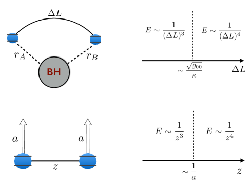
Figure 1: (Color online) The Casimir-Polder interaction between two atoms placed close to a black-hole horizon, displays the same non-thermal scaling behaviour as a function of the interatomic distance occurring for two relativistically uniformly accelerated atoms in a flat spacetime marino (Rindler metric). The characteristic crossover distance is in the former case proportional to the inverse of the surface gravity $\kappa$, while in the second case to the inverse of the proper acceleration $a$. Instead of the thermal scaling ($1/(\Delta L)^{2}$ or $1/z^{2}$) expected from the thermal Hawking/Unruh radiation, the Casimir interaction decreases faster to zero at large distances ($1/(\Delta L)^{4}$ or $1/z^{4}$) as a result of further distance-dependent contributions coming from the non-inertial character of the background metric. For short distances ($\Delta L\ll\sqrt{g_{00}}/\kappa$ or $z\ll 1/a$), the Casimir interatomic interaction is, instead, at leading order equivalent to its zero-temperature expression.

with $\tilde{\Delta}^{B}$ given by expression (33). Also in this case, there is no signature of the thermal distribution function in the expression for the radiation-reaction contribution. From these quantities, it is easy to see that the radiation-reaction contribution is once again given by expression (36) in this limit. On the other hand, for the vacuum-fluctuation contribution, one has (in the limit $t-t_{0}\to\infty$)

$$(\delta E)^{A}_{g,\textrm{vf}} \approx \frac{\lambda^{4}}{2048\pi^{4}\beta|\omega_{A}|^{2}}\frac{g_{00}}{(\Delta L)^{2}\,(1+(\kappa(r)\Delta L/2)^{2})}\,\left\{4\pi^{2}+2\pi\beta|\omega_{A}|\left[\pi\coth\left(\frac{\beta|\omega_{A}|}{2}\right)-i\Phi\left(e^{-\frac{4\pi d_{1}}{\beta}},1,\frac{i\beta|\omega_{A}|}{2\pi}\right)\right.\right.$$ (55)

$$+ \,\left.\left.i\Phi\left(e^{-\frac{4\pi d_{1}}{\beta}},1,-\frac{i\beta|\omega_{A}|}{2\pi}\right)\right]+\beta^{2}|\omega_{A}|^{2}\left[-\psi^{(1)}\left(\frac{i\beta|\omega_{A}|}{2\pi}\right)-\psi^{(1)}\left(-\frac{i\beta|\omega_{A}|}{2\pi}\right)\right.\right.$$

$$+ \,\left.\left.\Phi\left(e^{-\frac{4\pi d_{1}}{\beta}},2,\frac{i\beta|\omega_{A}|}{2\pi}\right)+\Phi\left(e^{-\frac{4\pi d_{1}}{\beta}},2,-\frac{i\beta|\omega_{A}|}{2\pi}\right)\right]\right\}.$$

As above, in the limit $\beta\omega_{A}\gg 1$, the Casimir-Polder energy is given by the vacuum-fluctuation contribution,

$$E_{\rm CP}\approx(\delta E)^{A}_{g,\textrm{vf}} \approx \frac{\lambda^{4}}{1024\pi^{2}\beta|\omega_{A}|^{2}}\frac{g_{00}}{(\Delta L)^{2}\,(1+(\kappa(r)\Delta L/2)^{2})}$$ (56)

$$\times \,\left[\beta|\omega_{A}|-4\coth\left(\frac{2\pi d_{1}}{\beta}\right)\right].$$

For $\kappa(r)\Delta L\ll 1$, we obtain the same results as above (considering gravitational-redshift effects), namely the vacuum-fluctuation contribution to the Casimir-Polder interaction near the event horizon exhibits, at the lowest order in $\kappa(r)\Delta L$, a scaling with the interatomic distance, characteristic of the finite temperature case. However, when $\kappa(r)\Delta L\gg 1$, one gets

$$(\delta E)^{A}_{g,\textrm{vf}}\approx\frac{\lambda^{4}\,\kappa^{2}}{256\pi^{2}|\omega_{A}|}\frac{1}{(\kappa(r)\Delta L)^{4}}-\frac{\lambda^{4}\kappa^{4}}{256\pi^{4}|\omega_{A}|^{2}}\frac{\beta}{(\kappa(r)\Delta L)^{4}}.$$ (57)

Hence, taking into account the radiation reaction contribution given by Eq. (38), one has that

$$E_{CP}\approx-\frac{\lambda^{4}\kappa^{4}}{256\pi^{4}|\omega_{A}|^{2}}\frac{\beta}{(\kappa(r)\Delta L)^{4}}.$$ (58)

The scaling of the Casimir energy (58) is in line with the conclusions of Ref. marino where the scaling of the Casimir-Polder force has been computed for two uniformly relativistic accelerating atoms. In particular, for interatomic distances larger than the typical length scale $1/\kappa(r)$, where the metric (and accordingly the field correlation functions) displays a strong noninertial character, the thermal scaling is deformed, and a novel scaling form for the Casimir-Polder interaction energy sets in. In close parallel, in Ref. marino it has been shown that this non-thermal scaling, $1/z^{4}$, of the Casimir interaction as a function of the interatomic distance $z$, occurs at distances larger than $\sim 1/a$, with $a$ the proper acceleration of the two atoms. The feature of having analogue scalings and the acceleration replaced by the surface gravity is expected on the basis of the equivalence of the Rindler metric with the Schwarzschild one, when the atoms are located close to the black hole horizon. The interpretation follows again the features discussed in the case of the Boulware vacuum: On the top of a thermal scaling regulated by the Hawking temperature $T$, additional factors depending on interatomic distance enter the Casimir interaction to implement the noninertial character of the background metric. Once again, this is a direct consequence of a change in the scaling of response ($\Delta$) and correlation functions ($D$), which is provoked by curvature corrections to the correlation functions at large enough distances where gravity effects are more pronounced.

The analogy between the nonthermal character of Casimir interaction in a Rindler and Schwarzschild background constitutes the central result of our work, and we summarize a comparison between these two cases in Fig. 1.

III.3 Unruh vacuum

The Unruh vacuum state is the adequate choice of vacuum state relevant for the gravitational collapse of a massive body sciama ; unruh . At spatial infinity, this vacuum depicts an outgoing flux of black-body radiation at the black-hole temperature.

By inserting Eq. (65) from the Appendix in Eqs. (10) and (11) one obtains the associated symmetric and response correlation functions, respectively. Not surprisingly, we obtain similar results as above within the same asymptotic limits. For instance, for $r_{A},r_{B}\to\infty$, one can easily prove that $(\delta E)^{A}_{g,\textrm{vf}}$ is given by Eq. (18), whereas $(\delta E)^{A}_{g,\textrm{rr}}$ is given by expression (19). In other words, one obtains the same results as in the Boulware vacuum at spatial infinity. In turn, with $r_{A},r_{B}\to 2GM$, one has that $(\delta E)^{A}_{g,\textrm{vf}}$ and $(\delta E)^{A}_{g,\textrm{rr}}$ are given, respectively, by Eqs. (53) and (31). That is, one obtains the same results as in the Hartle-Hawking vacuum near the event horizon.

IV Conclusions and Perspectives

We have discussed the contributions of vacuum fluctuations and radiation reaction to the Casimir-Polder forces between two identical atoms in Schwarzschild spacetime. We have shown how the distance-dependent radiative shifts of atoms in their ground states are modified when the atoms are placed near and far away from the black hole as well as when the quantum field is prepared in the Boulware, Hartle-Hawking, and Unruh vacuum states. Our findings generalize, in particular, the mechanism discussed in Ref. marino for two uniformly relativistic accelerated atoms: The Casimir-Polder interaction exhibits a transition between different scaling behaviors (thermal and nonthermal like) at a characteristic length associated with the mass of the black hole. This effect is pronounced close to the event horizon, and it originates from the noninertial character of the background metric, which provides further distance-dependent corrections to the otherwise expected thermal (at Hawking temperature) scaling of the Casimir interaction energy. Furthermore, close to the black hole, where the Schwarzschild metric takes the form of the Rindler line element, we find the same qualitative scaling as was found in Ref. marino for two relativistically uniformly accelerated two-level atoms.

There have been several investigations of quantum electrodynamic effects in a curved spacetime. Indeed, there is a number of discussions of the behavior of a scalar field (such as the Higgs particle) in the vicinity of strong gravitational sources onofrio1 . In turn, Ref. referee considers the Higgs self-interaction in a perturbed FRW metric. On the other hand, proposals highlighting the potential of spectroscopic measurements near the surface of white dwarfs and neutron stars can be found in Refs. onofrio2 . In a similar spirit, radiative shifts of matter surrounding a black hole might be significantly altered by the qualitative distance-dependent corrections discussed in this work. In this way the present results provide an indirect confirmation of corrections to the scaling of Casimir-Polder forces in accelerated backgrounds.

The formulae for the vacuum fluctuation and radiation reaction terms at fourth order in perturbation theory constitute a promising tool to compute Casimir interactions for ground-state atoms in other more complicated settings.

It would be interesting to generalize our results to other situations where quantum aspects of the gravitational field are of relevance. The first example is the study of gedanken experiments like the one discussed in UW82 , in which a box is lowered towards the event horizon. Quantum effects are there important to guarantee the validity of the Generalized Second Law of black hole mechanics. The second example is the Kerr black hole (see e.g. wheeler ). In contrast to a Schwarzschild black hole, it has a region called ergosphere in which static observers cannot exist. The calculation of Casimir-Polder energies near or in this region are of interest, but could also be of astrophysical relevance because observed black holes (such as the supermassive black hole with $4.3\times 10^{6}M_{\odot}$ in the center of the Milky Way) all have accretion disks of matter around them. Finally, the behavior of Casimir-Polder forces near cosmological horizons (de Sitter case) or in situations with both cosmological and black hole horizons (Schwarzschild-de Sitter case) GH77 ; FGK could turn out to be of conceptual interest. All of this would boost out knowledge about the intriguing features that appear when quantum theory and gravitational physics are intertwined.

acknowlegements

CK and JM thank Bill Unruh for an interesting discussion. JM thanks A. Noto, R. Passante, L. Rizzuto, S. Spagnolo for collaboration and discussions on closely related research topics. This work was partially supported by ‘Conselho Nacional de Desenvolvimento Cientifico e Tecnológico’ (CNPq, Brazil). JM acknowledges support from the Alexander von Humboldt foundation.

Appendix A Correlation functions of the scalar field in Schwarzschild spacetime

Here we present the correlation function of the quantum scalar field in Schwarzschild spacetime (for more details we refer the reader to frolov ; candelas and references cited therein). The Lagrangian density is given by

$$S=\frac{1}{2}\,\int d^{4}x\,\sqrt{-g}\,g^{\alpha\beta}\varphi_{,\alpha}\varphi_{,\beta}.$$ (59)

In the exterior region of Schwarzschild spacetime, a complete set of normalized basis functions for the massless scalar field is

$$u_{\omega lmn}(x)=\frac{1}{\sqrt{4\pi\omega}}\,R^{(n)}_{\omega l}(r)Y_{lm}\,e^{-i\omega t},$$ (60)

where the label $n$ distinguishes between modes incoming from past null infinity ${\cal J}^{-}$ (hereafter denoted by $n=\leftarrow$) and modes going out from the past horizon ${\cal H}^{-}$ (hereafter denoted by $n=\rightarrow$). One has the asymptotic forms:

$$\overrightarrow{R}_{\omega l}(r) \sim r^{-1}\,e^{i\omega r_{*}}+\overrightarrow{{\cal R}}_{l}(\omega)\,r^{-1}\,e^{-i\omega r_{*}},\,\,\,r\to 2GM$$

$$\overrightarrow{R}_{\omega l}(r) \sim \overrightarrow{{\cal T}}_{l}(\omega)\,r^{-1}\,e^{i\omega r_{*}},\,\,\,r\to\infty$$

$$\overleftarrow{R}_{\omega l}(r) \sim \overleftarrow{{\cal T}}_{l}(\omega)\,r^{-1}\,e^{-i\omega r_{*}},\,\,\,r\to 2GM$$

$$\overleftarrow{R}_{\omega l}(r) \sim r^{-1}\,e^{-i\omega r_{*}}+\overleftarrow{{\cal R}}_{l}(\omega)\,r^{-1}\,e^{i\omega r_{*}},\,\,\,r\to\infty,$$ (61)

where $r_{*}=r+2GM\ln(r/2GM-1)$ is the Regge-Wheeler tortoise coordinate, and ${\cal R}$ and ${\cal T}$ are the usual reflection and transmission coefficients, respectively, with the following properties

$$\overrightarrow{{\cal T}}_{l}(\omega) = \overleftarrow{{\cal T}}_{l}(\omega)={\cal T}_{l}(\omega),$$

$$|\overrightarrow{{\cal R}}_{l}(\omega)| = |\overleftarrow{{\cal R}}_{l}(\omega)|,$$

$$1-|\overrightarrow{{\cal R}}_{l}(\omega)|^{2} = 1-|\overleftarrow{{\cal R}}_{l}(\omega)|^{2}=|{\cal T}_{l}(\omega)|^{2},$$

$$\overrightarrow{{\cal R}}_{l}^{*}(\omega){\cal T}_{l}(\omega) = -{\cal T}^{*}_{l}(\omega)\overleftarrow{{\cal R}}_{l}(\omega).$$ (62)

The positive frequency Wightman functions associated with the Boulware vacuum $|0_{B}\rangle$, the Hartle-Hawking vacuum $|0_{H}\rangle$, and the Unruh vacuum $|0_{U}\rangle$ are given, respectively, by

$$\langle 0_{B}|\varphi(x)\varphi(x^{\prime})|0_{B}\rangle = \sum_{lm}\,\int_{0}^{\infty}\,\frac{d\omega}{4\pi\omega}\,e^{-i\omega(t-t^{\prime})}Y_{lm}(\theta,\phi)Y^{*}_{lm}(\theta^{\prime},\phi^{\prime})$$ (63)

$$\times \,\left[\overrightarrow{R}_{\omega l}(r)\overrightarrow{R}^{*}_{\omega l}(r^{\prime})+\overleftarrow{R}_{\omega l}(r)\overleftarrow{R}^{*}_{\omega l}(r^{\prime})\right],$$

$$\langle 0_{H}|\varphi(x)\varphi(x^{\prime})|0_{H}\rangle = \sum_{lm}\,\int_{-\infty}^{\infty}\,\frac{d\omega}{4\pi\omega}\,\Biggl{[}e^{-i\omega(t-t^{\prime})}Y_{lm}(\theta,\phi)Y^{*}_{lm}(\theta^{\prime},\phi^{\prime})\frac{\overrightarrow{R}_{\omega l}(r)\overrightarrow{R}^{*}_{\omega l}(r^{\prime})}{1-e^{-2\pi\omega/\kappa}}$$ (64)

$$+ e^{i\omega(t-t^{\prime})}Y^{*}_{lm}(\theta,\phi)Y_{lm}(\theta^{\prime},\phi^{\prime})\frac{\overleftarrow{R}^{*}_{\omega l}(r)\overleftarrow{R}_{\omega l}(r^{\prime})}{e^{2\pi\omega/\kappa}-1}\Biggr{]},$$

and

$$\langle 0_{U}|\varphi(x)\varphi(x^{\prime})|0_{U}\rangle = \sum_{lm}\,\int_{-\infty}^{\infty}\,\frac{d\omega}{4\pi\omega}\,e^{-i\omega(t-t^{\prime})}Y_{lm}(\theta,\phi)Y^{*}_{lm}(\theta^{\prime},\phi^{\prime})$$ (65)

$$\times \,\left[\frac{\overrightarrow{R}_{\omega l}(r)\overrightarrow{R}^{*}_{\omega l}(r^{\prime})}{1-e^{-2\pi\omega/\kappa}}+\theta(\omega)\overleftarrow{R}_{\omega l}(r)\overleftarrow{R}^{*}_{\omega l}(r^{\prime})\right],$$

where $\kappa=1/4GM$ is the surface gravity of the black hole birrel .

Let us now present the mode summations in the asymptotic regions $r\to 2GM$ and $r\to\infty$. At fixed radial distances $r$ and $r^{\prime}$, the correlation function of the field in the Boulware vacuum can be written as

$$\langle 0_{B}|\varphi(x)\varphi(x^{\prime})|0_{B}\rangle = \frac{1}{16\pi^{2}}\sum_{l=0}^{\infty}\,\int_{0}^{\infty}\,\frac{d\omega}{\omega}\,e^{-i\omega(t-t^{\prime})}(2l+1)\,P_{l}(\hat{r}\cdot\hat{r}^{\prime})$$ (66)

$$\times \,\left[\overrightarrow{R}^{(1)}_{\omega l}(r)\overrightarrow{R}^{(1*)}_{\omega l}(r^{\prime})+\overleftarrow{R}^{(1)}_{\omega l}(r)\overleftarrow{R}^{(1*)}_{\omega l}(r^{\prime})\right].$$

where we have used the addition theorem for the spherical harmonics, and $\hat{r}$ and $\hat{r}^{\prime}$ are two unit vectors with spherical coordinates $(\theta,\phi)$ and $(\theta^{\prime},\phi^{\prime})$. In general, one has

$$\sum_{l=0}^{\infty}(2l+1)\,P_{l}(\hat{r}\cdot\hat{r}^{\prime})\overrightarrow{R}_{\omega l}(r)\overrightarrow{R}^{*}_{\omega l}(r^{\prime})\approx\sum_{l=0}^{\infty}\frac{(2l+1)\,P_{l}(\hat{r}\cdot\hat{r}^{\prime})|{\cal T}_{l}(\omega)|^{2}e^{i\omega(r_{*}-r^{\prime}_{*})}}{rr^{\prime}},\,\,\,r,r^{\prime}\to\infty.$$ (67)

and for ${\bf x}={\bf x}^{\prime}$ we get ($P_{l}(1)=1$):

$$\sum_{l=0}^{\infty}(2l+1)|\overrightarrow{R}_{\omega l}|^{2}\approx\sum_{l=0}^{\infty}\frac{(2l+1)|{\cal T}_{l}(\omega)|^{2}}{r^{2}},\,\,\,r\to\infty.$$ (68)

In order to estimate the remaining sum, it is an important benchmark to recall that the above correlation function should agree at large radii with the correlation function of the scalar field in the Minkowski vacuum. Therefore, for $r,r^{\prime}\to\infty$, one gets

$$\sum_{l=0}^{\infty}(2l+1)\,P_{l}(\hat{r}\cdot\hat{r}^{\prime})\overleftarrow{R}_{\omega l}(r)\overleftarrow{R}^{*}_{\omega l}(r^{\prime})$$ (69)

$$\approx 4\omega\,\frac{\sin\left(\omega|{\bf x}-{\bf x}^{\prime}|\right)}{|{\bf x}-{\bf x}^{\prime}|},\,\,\,r,r^{\prime}\to\infty,$$

and in conclusion, for ${\bf x}={\bf x}^{\prime}$

$$\sum_{l=0}^{\infty}(2l+1)|\overleftarrow{R}_{\omega l}|^{2}\approx 4\omega^{2},\,\,\,r\to\infty.$$ (70)

Let us evaluate the mode sums in the region $r\approx 2GM$. We begin by defining $\zeta^{2}=r/2GM-1$ and $q=4GM\omega$. With these definitions, one can prove that $\overrightarrow{R}_{\omega l}$ obeys an equation that has the following approximate form:

$$\left[\zeta^{2}\frac{d^{2}}{d\zeta^{2}}+\zeta\frac{d}{d\zeta}+\left(q^{2}-(2l\zeta)^{2}\right)\right]\overrightarrow{R}_{\omega l}(\zeta)=0,$$ (71)

where we have approximated $l(l+1)\zeta^{2}\approx(l\zeta)^{2}$ since $\zeta\sim 0$. This is just the usual Bessel differential equation whose general solution can be expressed in terms of the modified Bessel functions:

$$\overrightarrow{R}_{\omega l}\big{|}_{r\to 2GM}\sim c_{l}K_{iq}(2l\zeta)+d_{l}I_{-iq}(2l\zeta).$$ (72)

As $l\to\infty$ for fixed $\zeta$, the radial function tends to zero; $r$ lies in the region in which the effective potential for the radial function is large. Hence $d_{l}$ is an exponentially small function of $l$ for large $l$ and the second term in equation (72) may be neglected in comparison with that of the first term in (72). The coefficient $c_{l}$ may be determined by comparing the asymptotic result $z\to 0$ for $K_{\nu}(z)$ with the asymptotic solution

$$\overrightarrow{R}_{\omega l}(r)\sim e^{i\omega r_{*}}\,r^{-1}+\overrightarrow{{\cal R}}_{l}(\omega)e^{-i\omega r_{*}}\,r^{-1},\,\,\,r\to 2GM.$$

One finds that

$$c_{l}\sim\frac{e^{iq/2}\,l^{-iq}}{GM\Gamma(-iq)}.$$ (73)

Therefore, at leading order we have

$$\sum_{l=0}^{\infty}(2l+1)\,P_{l}(\hat{r}\cdot\hat{r}^{\prime})\overrightarrow{R}_{\omega l}(r)\overrightarrow{R}^{*}_{\omega l}(r^{\prime})\approx\frac{1}{GM^{2}\Gamma(iq)\Gamma(-iq)}\sum_{l}^{\infty}(2l+1)P_{l}(\cos\gamma)\,K_{iq}(2l\zeta)K_{iq}(2l\zeta^{\prime})$$

$$\approx\frac{8GM\omega\sinh(4\pi GM\omega)}{\pi GM^{2}}\int_{0}^{\infty}dl\,l\,J_{0}(l\gamma)\,K_{iq}\left(2l\sqrt{g_{00}(r)}\right)K_{iq}\left(2l\sqrt{g_{00}(r^{\prime})}\right),\,\,\,r,r^{\prime}\to 2GM$$ (74)

where $g_{00}=(1-2GM/r)$, $\cos\gamma=\hat{r}\cdot\hat{r}^{\prime}=\cos\theta\cos\theta^{\prime}+\sin\theta\sin\theta^{\prime}\cos(\phi-\phi^{\prime})$, and we have used abram

$$\Gamma(iq)\Gamma(-iq)=\frac{\pi}{q\sinh(\pi q)},$$

together with the asymptotic result:

$$P_{\nu}\left(\cos\frac{x}{\nu}\right)\approx J_{0}(x)+{\cal O}(\nu^{-1}),$$

in which $J_{\mu}(x)$ is a Bessel function of the first kind. Considering that $r\approx r^{\prime}$ (but ${\bf\hat{r}}\neq{\bf\hat{r}}^{\prime}$), one may resort to the result prud :

$$\int_{0}^{\infty}dx\,xJ_{0}(ax)[K_{iq}(2bx)]^{2}=\frac{i\pi\text{csch}(\pi q)\sin\left(2q\sinh^{-1}\left(\frac{a}{4b}\right)\right)}{a^{2}\sqrt{-\frac{16b^{2}}{a^{2}}-1}},$$

where we assume a small positive imaginary part for $a$ so that the integral converges. Therefore, as a next step we find

$$\sum_{l=0}^{\infty}(2l+1)\,P_{l}({\bf\hat{r}}\cdot{\bf\hat{r}}^{\prime})\overrightarrow{R}_{\omega l}(r)\overrightarrow{R}^{*}_{\omega l}(r^{\prime})\approx\frac{4\omega}{\sqrt{g_{00}}}\,\frac{\sin\left[(2\omega/\kappa)\sinh^{-1}\left(\frac{\kappa(r)\Delta L}{2}\right)\right]}{\Delta L\sqrt{1+(\kappa(r)\Delta L/2)^{2}}},\,\,\,r,r^{\prime}\to 2GM,$$

(75)

where $\kappa(r)=\kappa/\sqrt{g_{00}(r)}$ and $\Delta L=r_{s}\gamma$ are defined as above. For ${\bf x}={\bf x}^{\prime}$ we find

$$\sum_{l=0}^{\infty}(2l+1)\,|\overrightarrow{R}^{(1)}_{\omega l}|^{2}\approx\frac{4\omega^{2}}{g_{00}},\,\,\,r\to 2GM,$$ (76)

where we have used that prud

$$\frac{2}{\Gamma(iq)\Gamma(-iq)}\int_{0}^{\infty}dt\,t\,[K_{iq}\left(2tx\right)]^{2}=\frac{q^{2}}{4x^{2}}.$$

The other mode sum in the region $r\to 2GM$ can be easily estimated:

$$\sum_{l=0}^{\infty}(2l+1)\,P_{l}(\hat{r}\cdot\hat{r}^{\prime})\overleftarrow{R}_{\omega l}(r)\overleftarrow{R}^{*}_{\omega l}(r^{\prime})\approx\sum_{l=0}^{\infty}\frac{(2l+1)P_{l}(\hat{r}\cdot\hat{r}^{\prime})|{\cal T}_{l}(\omega)|^{2}e^{-i\omega(r_{*}-r^{\prime}_{*})}}{(2GM)^{2}},\,\,\,r,r^{\prime}\to 2GM,$$ (77)

which for ${\bf x}={\bf x}^{\prime}$ reads

$$\sum_{l=0}^{\infty}(2l+1)|\overleftarrow{R}_{\omega l}|^{2}\approx\sum_{l=0}^{\infty}\frac{(2l+1)|{\cal T}_{l}(\omega)|^{2}}{(2GM)^{2}},\,\,\,r\to 2GM.$$ (78)

References

• (1) C. Kiefer, Quantum Gravity, International Series of Monographs on Physics 155, third edition (Oxford University Press, Oxford, 2012).
• (2) N. D. Birrell and P. C. W. Davis, Quantum Fields in Curved Space (Cambridge University Press, Cambridge, 1982); L. E. Parker and D. J. Toms, Quantum Field Theory in Curved Spacetime: Quantized Fields and Gravity (Cambridge University Press, Cambridge, 2009).
• (3) V. P. Frolov and I. D. Novikov, Black Hole Physics: Basic Concepts and New Developments (Kluwer Academic Publishers, Dordrecht, 1998).
• (4) S. W. Hawking, Commun. Math. Phys. 43, 199 (1975); Erratum: ibid. 46, 206 (1976).
• (5) D. Harlow, Rev. Mod. Phys. 88, 15002 (2016).
• (6) H. B. G. Casimir, Proc. Kon. Ned. Akad. Wet. 51, 793 (1948).
• (7) G. Plunien, B. Müller, and W. Greiner, Phys. Rep. 134, 87 (1986).
• (8) A. A. Grib, S. G. Mamayev, and V. M. Mostepanenko, Vacuum Quantum Effects in Strong Fields (Friedman Laboratory Publishing, St. Petersburg, 1994).
• (9) M. Bordag, U. Mohideen, and V. M. Mostepanenko, Phys. Rep. 353, 1 (2001).
• (10) K. A. Milton,The Casimir Effect : Physical Manifestation of Zero-Point Energy (World Scientific, Singapore, 2001).
• (11) P. W. Milonni, Phys. Rep. 25, 1 (1976).
• (12) S. K. Lamoreaux, Phys. Rev. Lett. 78, 5 (1997); U. Mohideen and A. Roy, Phys. Rev. Lett. 81, 4549 (1998); G. Bressi, G. Carugno, R. Onofrio, and G. Ruoso, Phys. Rev. Lett. 88, 041804 (2002); R. S. Decca, E. Fischbach, G. L. Klimchitskaya, D. E. Krause, D. López, and V. M. Mostepanenko, Phys. Rev. D 68, 116003 (2003); G. L. Klimchitskaya, U. Mohideen, and V. M. Mostepanenko, Rev. Mod. Phys. 81, 1827 (2009).
• (13) H. B. G. Casimir and D. Polder, Phys. Rev. 73, 360 (1948).
• (14) T. Cysne, W. J. M. Kort-Kamp, D. Oliver, F. A. Pinheiro, F. S. S. Rosa, and C. Farina, Phys. Rev. A 90, 052511 (2014).
• (15) S. A. Fulling, K. A. Milton, P. Parashar, A. Romeo, K. V. Shajesh, and J. Wagner, Phys. Rev. D 76, 025004 (2007); K. A. Milton, P. Parashar, K. V. Shajesh, and J. Wagner, J. Phys. A: Math. Theor. 40, 10935 (2007); K. V. Shajesh, K. A. Milton, P. Parashar, and J. A. Wagner, J. Phys. A: Math. Theor. 41, 164058 (2008); K. A. Milton, K. V. Shajesh, S. A. Fulling, and P. Parashar, Phys. Rev. D 89, 064027 (2014).
• (16) J. Dalibard, J. Dupont-Roc, and C. Cohen-Tannoudji, J. Phys. (Paris) 43, 1617 (1982).
• (17) J. Dalibard, J. Dupont-Roc, and C. Cohen-Tannoudji, J. Phys. (Paris) 45, 637 (1984).
• (18) J. Audretsch and R. Müller, Phys. Rev. A 50, 1755 (1994); R. Passante, ibid. 57, 1590 (1998); H. Yu and S. Lu, ibid. 72, 064022 (2005); Z. Zhu, H. Yu, and S. Lu, ibid. 73, 107501 (2006); L. Rizzuto, Phys. Rev. A 76, 062114 (2007); Z. Zhu and H. Hu, Phys. Lett. B 645, 459 (2007); L. Rizzuto and S. Spagnolo, Phys. Rev. A 79, 062110 (2009); J. Zhang and H. Yu, ibid. 84, 042103 (2011).
• (19) G. Menezes and N. F. Svaiter, Phys. Rev. A 92, 062131 (2015).
• (20) G. Menezes and N. F. Svaiter, Phys. Rev. A 93, 052117 (2016).
• (21) G. Menezes, Phys. Rev. D 94, 105008 (2016).
• (22) J. Marino, A. Noto, and R. Passante, Phys. Rev. Lett. 113, 020403 (2014).
• (23) A. Noto, Non-equilibrium Casimir interactions: from dynamical to thermal effects, PhD thesis, University of Palermo and University of Montpellier (2016); J. Marino, A. Noto, R. Passante, and W. Zhou, in preparation (2017)
• (24) L. Rizzuto, et al. Phys. Rev. A 94, 012121 (2016); W. Zhou, R. Passante, and L. Rizzuto, Phys. Rev. D 94, 105025 (2016).
• (25) J. Zhang and H. Yu, Phys. Rev. A 88, 064501 (2013).
• (26) C. W. Misner, K. S. Thorne, and J. A. Wheeler, Gravitation (W. H. Freeman, San Francisco, 1973).
• (27) D. G. Boulware, Phys. Rev. D 11, 1404 (1975); ibid. 12, 350 (1975).
• (28) D. W. Sciama, P. Candelas, and D. Deutsch, Adv. Phys 30, 327 (1981).
• (29) R. Courant and D. Hilbert, Methods of Mathematical Physics (Wiley-Interscience, New York, 1962) Volume I.
• (30) M. Abramowitz and I. A. Stegun, Handbook of Mathematical Functions with Formulas, Graphs, and Mathematical Tables (Dover, New York, 1972).
• (31) J. B. Hartle and S. W. Hawking, Phys. Rev. D 13, 2188 (1976).
• (32) W. G. Unruh, Phys. Rev. D 14, 870 (1976).
• (33) P. Candelas, Phys. Rev. D 21, 2185 (1980).
• (34) A. P. Prudnikov, Yu A. Brychkov, and O. I. Marichev, Integrals and Series (Gordon and Breach, London, 1986) vols. 1 and 2.
• (35) R. Onofrio, Phys. Rev. D 82, 065008 (2010); P. O. Kazinski, Phys. Rev. D 85, 044008 (2012).
• (36) F. D. Albareti, A. L. Maroto, and F. Prada, Phys. Rev. D 95, 044030 (2017).
• (37) G. A. Wegner, R. Onofrio, Astrophys. J. 791, 125 (2014); G. A. Wegner, R. Onofrio, Eur. Phys. J. C 75, 307 (2015).
• (38) W. G. Unruh and R. M. Wald, Phys. Rev. D 25, 942 (1982).
• (39) G. W. Gibbons and S. W. Hawking, Phys. Rev. D 15, 2738 (1977).
• (40) A. Franzen, S. Gutti, and C. Kiefer, Class. Quantum Grav. 27, 015011 (2010).