Massively parallel Lattice Boltzmann codes
on large GPU clusters

Abstract

This paper describes a massively parallel code for a state-of-the art thermal Lattice Boltzmann method. Our code has been carefully optimized for performance on one GPU and to have a good scaling behavior extending to a large number of GPUs. Versions of this code have been already used for large-scale studies of convective turbulence.

GPUs are becoming increasingly popular in HPC applications, as they are able to deliver higher performance than traditional processors. Writing efficient programs for large clusters is not an easy task as codes must adapt to increasingly parallel architectures, and the overheads of node-to-node communications must be properly handled.

We describe the structure of our code, discussing several key design choices that were guided by theoretical models of performance and experimental benchmarks. We present an extensive set of performance measurements and identify the corresponding main bottlenecks; finally we compare the results of our GPU code with those measured on other currently available high performance processors. Our results are a production-grade code able to deliver a sustained performance of several tens of Tflops as well as a design and optimization methodology that can be used for the development of other high performance applications for computational physics.

1 Overview

High Performance Computing (HPC) has seen in recent years an increasingly large role played by Graphics Processing Units (GPUs), offering a performance level significantly larger than traditional processors. GPUs have many slim processing units on a single chip and perform in parallel a very large number (${\cal O}(1000)$) of operations on a correspondingly large number of operands. While not limited to such cases, this structure is obviously efficient for algorithms offering a large amount of available parallelism; in these cases it is possible to identify and concurrently schedule many operations on data items that have no dependencies among them. This is often the case for so-called stencil codes. Stencil codes are typically used to model systems defined on regular lattices; they process data elements associated to each lattice site applying some regular sequence of mathematical operations to data belonging to a fixed pattern of neighboring cells. General implementation and optimization of stencils on GPUs has been extensively studied by many authors, [1, 2, 3, 4]. This approach is appropriate also for several computational Grand Challenge applications, such as Lattice QCD (LQCD), or Computational Fluid-dynamics using the Lattice Boltzmann method (LBM). Correspondingly, a large effort has gone in recent years in porting and optimizing for GPUs codes and libraries relevant for these applications [5, 6, 7, 8].

Interesting results have been reported, exhibiting significant performance levels obtained on one or just a small number of GPUs. However, the number of very large scale computational applications heavily relying on GPUs is still limited, partly because the high performance of GPUs makes node-to-node communication bandwidth in a large machine a performance bottleneck sooner (i.e. fewer nodes) than other platforms, limiting scaling behavior on a large number of nodes.

In the last few years, we have conducted a large and systematic analysis of several properties of convective turbulence, using as our computational tool a massively parallel GPU-based LBM code; physics results have been reported elsewhere (see [9] and references therein). After an early development, see [10, 11], and in parallel with physics simulations, our code has undergone a systematic process of further refinements, improving optimization strategies, adapting to new GPU generations and exploiting improved GPU-to-GPU communications tools.

In this paper we cover the computational aspects of this work, discussing the structure of the code, the optimization strategies appropriate to boost performances on just one GPU, and the possible approaches to improve the scaling behavior of the code on a large GPU cluster; we study and analyze in details a number of issues related to state-of-the-art computing systems based on GPUs, and identify the corresponding ways-out; in other words, what we offer here is an attempt at building a sound optimization approach for GPUs; while our analysis is based on a specific (but computationally relevant) application, we trust that our results may provide useful guidance for those adapting and optimizing a wider class of computational applications for GPU-based computing.

Analyses on the best options to port LBM codes on massively parallel systems have recently appeared [12], and detailed studies have focused on the impact on performance of several memory allocation and access strategies [13, 14, 15, 16]. Comparisons of results on several multi-core processors and GPUs have also been presented in [17, 18, 19, 20]. Here we improve and extend those results, further optimizing the codes and exploiting recent improvements in GPU-to-GPU data exchange.

This paper is structured as follows: the next section describes the LBM model that we consider; the following section reviews the architecture of GPU processors and GPU-based systems. This is followed by a detailed analysis of our optimization work, divided in two successive sections, considering first the single GPU case, and then parallelization on a large number of GPUs. We then discuss our performance results, including a comparison with similar codes optimized for different CPU architectures; our conclusions and outlook end the paper. An appendix collects and annotates several critical code segments, better documenting our implementation choices.

2 Lattice Boltzmann methods

In this section, we sketchily introduce the computational method that we adopt, based on an advanced thermal Lattice Boltzmann scheme. LBM methods (see, e.g. [21] for an extended introduction) are discrete in both position and momentum spaces; they are based on the synthetic dynamics of populations sitting at the sites of a discrete lattice.

This computational method simulates the behavior of a compressible gas/fluid. The Thermal-Kinetic description of a compressible gas/fluid of variable density, $\rho$, local velocity ${\bm{u}}$, internal energy, ${\cal K}$ and subject to a local body force density, ${\bm{g}}$, is given by the following equations:

$$\partial_{t}\rho+\partial_{i}(\rho u_{i})=0$$ (1)

$$\partial_{t}(\rho u_{k})+\partial_{i}(P_{ik})=\rho g_{k}$$ (2)

$$\partial_{t}{\cal K}+\frac{1}{2}\partial_{i}q_{i}=\rho g_{i}u_{i}$$ (3)

where $P_{ik}$ and $q_{i}$ are the momentum and energy fluxes.

In the continuum, one shows that it is possible to recover these equations, starting from a continuum Boltzmann Equations and introducing a suitable shift of the velocity and temperature fields entering in the local equilibrium [22], $f^{(eq)}({\bm{\xi}};\rho,T,{\bm{u}})\rightarrow{f}^{(eq)}({\bm{\xi}};\rho,{\bar{T}},{\bm{\bar{u}}})$. The new Boltzmann formulation is then:

$$\frac{\partial f}{\partial t}+{\bm{\xi}}\cdot{\bm{\nabla}}f=-\frac{1}{\tau}(f-{\ f}^{(eq)})\;$$ (4)

$${f}^{(eq)}({\bm{\xi}};\rho,\bar{T},\bar{\bm{u}})=\frac{\rho}{(2\pi{\bar{T}})^{D/2}}e^{-|{\bm{\xi}}-{\bm{\bar{u}}}|^{2}/2{\bar{T}}},$$ (5)

and the shifted local velocity and temperature take the following form $\bar{\bm{u}}={\bm{u}}+\tau{\bm{g}},~{}~{}\bar{T}=T-\tau^{2}g^{2}/D$ ($D$ is the space dimensionality).

The discretized counterpart of the continuum description (that we use in this paper) uses a set of fields $f_{l}(x,t)$ associated to the so-called populations; the latter can be visualized as pseudo-particles moving in appropriate directions on a discrete mesh (see Figure 1). In this paper we consider a 2D LBM algorithm, that uses 37 populations (a so called D2Q37 model), recently developed in [22, 23]. The master evolution equation in the discrete world is:

$$f_{l}({\bm{x}}+{\bm{c}}_{l}{\Delta t},t+{\Delta t})-f_{l}({\bm{x}},t)=-\frac{{\Delta t}}{\tau}\left(f_{l}({\bm{x}},t)-f_{l}^{(eq)}\right);$$ (6)

subscript $l$ runs over the discrete set of velocities, ${\bm{c}}_{l}$ (see again Figure 1) and equilibrium is expressed in terms of hydrodynamical fields on the lattice, ${f}_{l}^{(eq)}={f}_{l}^{(eq)}({\bm{x}},\rho,\bar{\bm{u}},\bar{T})$.

To first approximation, the macroscopic fields are defined in terms of the lattice Boltzmann populations: $\rho=\sum_{l}f_{l}$, $\rho{\bm{u}}=\sum_{l}{\bm{c}}_{l}f_{l}$, $D\rho T=\sum_{l}\left|{\bm{c}}_{l}-{\bm{u}}\right|^{2}f_{l}$. When going into all mathematical details, one finds that shifts and renormalizations have to be applied to the averaged hydrodinamical quantities to correct for lattice discretization effects. After performing these manipulations, one recovers the correct thermo-hydrodynamical equations:

$$D_{t}\rho=-\rho{\partial_{i}}u^{(H)}_{i}$$ (7)

$$\rho D_{t}u^{(H)}_{i}=-{\partial_{i}}p-\rho g\delta_{i,3}+\nu\partial_{jj}u^{(H)}_{i}$$ (8)

$$\rho c_{v}D_{t}T^{(H)}+p{\partial_{i}}u^{(H)}_{i}=k\partial_{ii}T^{(H)}$$ (9)

where we have introduced the material derivative, $D_{t}=\partial_{t}+u_{j}^{(H)}{\partial_{j}}$, neglected viscous dissipation in the heat equation and the superscript $H$ denotes the lattice-corrected quantities; $c_{v}$ is the specific heat at constant volume for an ideal gas $p=\rho T^{(H)}$, $\nu$ and $k$ are the transport coefficients.

The LBM model considered in this paper correctly reproduces the thermo-hydrodynamical equations of motions of a fluid in two dimensions, and automatically enforces the equation of state of a perfect gas ($p=\rho T$). This is a substantial improvement over simpler LBM schemes in two or three dimensions (e.g., D2Q9 or D3Q19) that regard the fluid as incompressible, and introduce ad hoc approximations (e.g., the Boussinesq approximation) to partially model the dependence of density on temperature, relevant for convection.

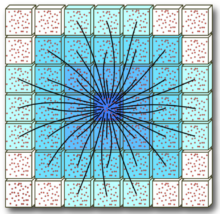
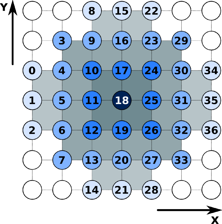
Figure 1: Left: Velocity vectors for populations in the D2Q37 model, associated to the lattice hop that they perform in the propagate phase. Right: each population is identified by an arbitrary label.

An LBM code starts with an initial assignment of the populations, in accordance with a given initial condition at $t=0$ on some spatial domain, and then iterates Eq. 6 for each point in the domain and for as many time-steps as needed; at each time step, populations hops from lattice-site to lattice-site and then incoming populations collide among one another. In this step populations mix and their values change accordingly. Boundary-conditions are enforced at the boundary of the integration domain after each time-step by appropriately modifying the population values at and close to the boundary.

From the computational point of view, the LBM approach offers a huge degree of available parallelism. Defining ${\bm{y}}={\bm{x}}+{\bm{c}}_{l}{\Delta t}$ and rewriting the main evolution equation as:

$$f_{l}({\bm{y}},t+{\Delta t})=f_{l}({\bm{y}}-{\bm{c}}_{l}{\Delta t},t)-\frac{{\Delta t}}{\tau}\left(f_{l}({\bm{y}}-{\bm{c}}_{l}{\Delta t},t)-f_{l}^{(eq)}\right)$$ (10)

one easily identifies the overall structure of the computation that evolves the system by one time step ${\Delta t}$; for each point ${\bm{y}}$ in the discrete grid one:

1. gathers from neighboring sites the values of the fields $f_{l}$ corresponding to populations drifting towards ${\bm{y}}$ with velocity ${\bm{c}}_{l}$ and then

2. performs all mathematical processing needed to compute the quantities appearing in the r.h.s. of Eq. (10), for each point in the grid.

Both steps above are completely uncorrelated for different lattice-points, so they can be computed in parallel according to any convenient schedule, as long as one makes sure that, for all grid points, step 1 is performed before step 2.

At each iteration of the loop over time, every lattice-point is processed applying in sequence the following three main kernels:

• propagate: for each lattice-site we move populations according to the pattern of Figure 1 left. This process does not perform any mathematics but only moves blocks of memory locations allocated at sparse addresses. It collects at each site all populations that will interact at the next computational phase (collide). In this step each site accesses the populations of the neighbor cells at distance up to 3 in the grid.

• bc adjusts values of the populations at the top and bottom edges of the lattice to enforce appropriate boundary conditions (e.g., a constant given temperature and zero velocity). This step is necessarily done after propagation, since the latter changes the value of the populations close to the boundary points and hence the macroscopic quantities that we must keep constant in time. At the right and left boundaries, we apply periodic boundary conditions. This is most easily done by allocating halo columns, additional storage where copies of the 3 (in our case) rightmost and leftmost columns of the lattice are placed before performing the propagate step. Points close to the right/left boundaries can then be processed as those in the bulk. If needed, boundary conditions could of course be enforced in the same way as we do for the top and bottom edges.

• collide performs all the mathematical steps associated to Eq. 10 in order to compute the population values at each lattice site at the new time step (this is called “collision”, in LBM jargon). Input data for this phase are the populations gathered by the previous propagate phase. This step is the truly floating point intensive section of the code; it uses only the population members of the site on which it operates, making the processing of different sites fully uncorrelated.

The computational price to price to pay for this very accurate physics model is that the implementation of the steps described above is much more complex than for simpler LBM models. More severe computational requirements in terms of memory bandwidth and floating-point throughput follow. Indeed, propagate implies accessing 37 neighbor cells to gather all populations, while collide requires $\approx 7000$ double-precision floating point operations per lattice point.

3 NVIDIA GPU Architectures

In this work we experiment with two recent generations of NVIDIA GPUs: the Tesla processors, C2050 and C2070, based on the GF100 GPU belonging to the Fermi generation, and the latest K20X, K40 and K80 processors, based on the Kepler architecture. The K20X uses a GK110 GPU, the K40 a GK110B GPU, and the K80 is a dual GK210 GPU. In the following we use interchangeably the name of the systems or that of the corresponding GPUs, unless ambiguities arise.

NVIDIA GPUs are multi-core processors. Processing units are called SM (Streaming Multiprocessors) on Fermi and SMX on Kepler (as they have enhanced capabilities). Each processing unit has 32 (Fermi) or 192 (Kepler) compute units called CUDA-cores in NVIDIA jargon; at each clock-cycle SMs executes multiple warps, i.e. groups of 32 operations called CUDA-threads which proceed in SIMT fashion .

At variance with CPU threads, context switches among active CUDA-threads are instantaneous due to maintaining many thread states. Typically one CUDA-thread processes one element of the data-set of the application. This helps exploit all available parallelism of the algorithm and hide latencies by switching among threads waiting for data coming from memory and threads ready to run. This structure has remained stable across both generations. Several enhancements are available in the more recent Kepler processors; for instance, Kepler has 256 32-bit registers addressable by each CUDA-thread (a $4X$ increase over Fermi) and each SMX has 65536 registers (a $2X$ increase). Kepler GPUs are also able to increase their clock frequency beyond the nominal value, if power and thermal constraints allow to do so (GPUBoost, in NVIDIA jargon).

Within each generation, minor differences occur: the C2050 and C2070 processors differ in the amount of available global memory; the K40 processor has more global memory than the K20 and slightly improves memory bandwidth and floating-point throughput; finally the K80 has two enhanced Kepler GPUs with more registers and shared memory than K20/K40 and extended GPUBoost features. The Tesla C2050 system has a peak performance of $\approx 1$ Tflops in single-precision (SP), and $\approx 500$ Gflops in double-precision (DP); on the Kepler K20 and K40, the peak SP (DP) performance is $\approx 5$ Tflops ($\approx 1.5$ Tflops), while on the K80 the aggregate performance of the two GPUs delivers a peak SP (DP) of $\approx 5.6$ Tflops ($\approx 1.9$ Tflops).

Fast access to memory strongly correlates with performance: peak bandwidth is $144$ GB/s for the C2050 and C2070 processors, and $250$ and $288$ GB/s respectively for the K20X and the K4 0;on the K80, the aggregate peak is $480$ GB/s. The memory system has an error detection and correction system (ECC) to increase reliability when running large codes. We have always used this feature, even if it slightly reduces available memory and bandwidth (e.g. on the Tesla C2050 available memory is reduced by $\approx 12\%$; for the propagate kernel measured bandwidth is reduced by $\approx 20\cdots 25$% ). For a more complete description, see [24, 25]; Table 1 summarizes just a few relevant parameters.

Table 1: Selected hardware features of the GPU systems considered in this paper: the C2050 and C2070 are based on the Fermi architecture, while the K20X, K40 and K80 follow the Kepler architecture.

	C2050 / C2070	K20X	K40	K80
GPU	GF100	GK110	GK110B	GK210	$\times$ 2
Number of SMs	16	14	15	13	$\times$ 2
Number of CUDA-cores	448	2688	2880	2496	$\times$ 2
Nominal clock frequency (MHz)	1.15	735	745	562
Nominal DP performance (Gflops)	515	1310	1430	935	$\times$ 2
Boosted clock frequency (MHz)	–	–	875	875
Boosted DP performance(Gflops)	–	–	1660	1455	$\times$ 2
Total available memory (GB)	3 / 6	6	12	12	$\times$ 2
Memory bus width (bit)	384	384	384	384	$\times$ 2
Peak mem. BW (ECC-off) (GB/s)	144	250	288	240	$\times$ 2
Max Power (Watt)	215	235	235	300

We have developed all our codes using CUDA-C [26], a GPU-specific programming language with several features intended to help exploit the parallelism available in the algorithm. A CUDA-C program consists of one or more functions that run either on the host, a standard CPU, or on a GPU. Functions with no (or limited) parallelism run on the host, while those exhibiting a large degree of data parallelism go onto the GPU. A CUDA-C program is a modified C (or C++) program including keyword extensions defining data parallel functions, called kernels. Kernel functions typically translate into a large number of threads, i.e. a large number of independent operations processing independent data items. Threads are grouped into blocks which in turn form the execution grid. The grid can be configured as a 1-, 2- or 3-dimensional array of blocks, each block is itself a 1-, 2- or 3-dimensional array of threads, running on the same SM, and sharing data through a fast shared memory. When all threads of a kernel complete their execution, the corresponding grid terminates. CUDA-threads run in parallel with CPU threads, so it is possible to overlap in time processing on the host and the accelerator. For our purposes this is useful to concurrently schedule computation and GPU-to-GPU communication.

4 Single-GPU Implementation

In this section we describe data-structures options, the overall organization of the code and optimizing features considering only one GPU. The extension to a multi-GPU cluster will be considered in the next section.

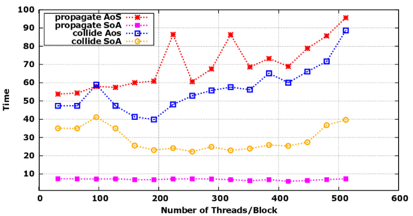
Figure 2: Execution times (arbitrary units) of the propagate and collide kernels as a function of the number of threads per block, using the AoS and SoA data layouts.

Data Structure Analysis

A major decision affecting the overall structure of the code has to do with the choice of an appropriate data organization, which has a strong impact on the ability of the system to fetch from memory all the data elements needed by the processor. In LBM popular data organizations are array of structures (AoS) or structure of arrays (SoA). With AoS, all populations associated to each lattice site are stored one after the other in memory; conversely, SoA stores data items corresponding to each population at all lattice sites one after the other. For serial computations on cache-based architectures, like traditional CPUs, the AoS scheme is preferable as it improves the locality of populations associated to each lattice point, and better suits the cache structure and hierarchy of these processors. On the other hand SoA is required for data parallelism computation typical of GPUs, since it allows to process data associated to several lattice sites in parallel and allows coalescing of memory accesses, that helps achieve high sustained memory bandwidth. This is substantiated in figure 2, showing a preliminary performance analysis of two critical kernels; propagate (a memory-bound kernel, see later for details) is at least a factor $5X$ faster using the SoA scheme, while collide (a compute-bound kernel) is roughly $2X$ faster.

Having settled for an SoA structure, we store the lattice in column-major order in the $Y$ direction (we arbitrarily select one of the two possible choices), and keep in memory two copies of the lattice. Code sections alternatively read one copy and write on the other copy; this technique is known as double-buffering. This helps maximize parallelism, allowing to map one thread per lattice site, and then processing all sites in parallel.

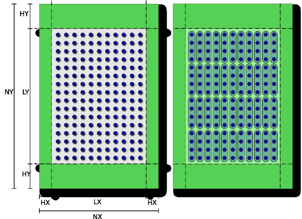
Figure 3: Left: Allocation of lattice data in global memory; green regions are the halo frames, the white area is the physical lattice. Right: sketchy view of the mapping of the lattice on CUDA thread-blocks and block-grids.

We surround the physical lattice by halo-columns and rows, see Figure 3: for a physical lattice of size $L_{x}\times L_{y}$, we allocate an array of $NX\times NY$ lattice points, $NX=H_{x}+L_{x}+H_{x}$, and $NY=H_{y}+L_{y}+H_{y}$. This makes the computation uniform for all sites and avoid thread divergences which break data-parallelism and degrade performances. The algorithm requires a halo-thickness of just 3 points, since populations move up to three sites at each time step. It is convenient to use a larger halo thickness in the $Y$ directions (Hy = 16), in order to keep data aligned (multiples of 32, the size of the warp, permit more efficient access through “coalescing”) and to maintain also cache-line alignment in multiples of 128 Bytes.

Code Organization

Our code starts on the host, and at each iteration four main steps execute: first the pbc kernel update halos, and then three kernels – propagate, bc and collide – perform the required computational tasks. Each kernel corresponds to a CUDA-C function.

For a single GPU implementation the pbc kernel updates only the left and right halos, as we enforce periodic boundary conditions along $X$; this amounts to copying data from the three right-most columns of the physical lattice to the left halo columns, and vice-versa. In this case, we move data stored at contiguous elements in memory, so we handle it by efficient CUDA-C memory-copy library functions. We make two calls to the cudaMemcpyAsync function; execution overlaps in time, substantially increasing performance.

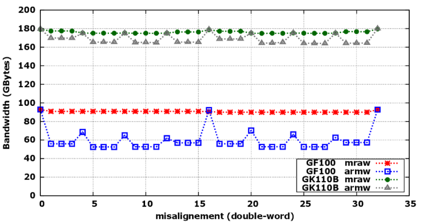
Figure 4: Performance (ECC enabled) of misaligned-read-aligned-write (mraw) and aligned-write-misaligned-read (armw) accesses on the C2050 (GF100 GPU), and K40 (GK110B GPU) systems.

The propagate and bc Kernels

The propagate kernel moves populations at each site according to the pattern shown in Figure 1. Two options are possible: i) push moves all populations of each lattice site to the appropriate neighbor sites; or ii) pull gathers populations from neighbor sites to each destination site. push performs aligned reads and misaligned writes, while the opposite happens in pull. In both cases, misaligned memory operations are needed. Figure 4 plots the measured bandwidth of a memory-copy kernel using misaligned reads and aligned writes (mraw) and vice-versa (armw). The mraw scheme is faster on both GPU generations even if the performance gain, large for the C2050 system, is smaller for the more recent K20 and K40 GPUs. This test obviously suggests to adopt the pull scheme.

For this kernel, each CUDA-block is configured as a unidimensional array of N_THREAD threads, processing data allocated at successive locations in memory, while the grid of blocks is a bi-dimensional array of ($L_{y}$/N_THREAD $\times$ $L_{x}$) blocks, see Figure 3, right. N_THREAD, in principle a free parameter, must be accurately tuned for performance: N_THREAD should be large enough because it translates in long and efficient memory access sequences. On the other hand, ($L_{y}$/N_THREAD $\times$ $L_{x}$) should also be large, because it translates into many independent sequences, so some sequence is almost always ready to execute while other are waiting for data incoming from memory. Figure 5 shows the impact of this parameter on performance, displaying the effective memory bandwidth as a function of the number of threads per block. We see that performance stabilizes to a reasonable level as long as ${\tt N\_THREAD}\geq 64$; on the C2050 processor, we reach a bandwidth of $\approx 85$ GB/s that increases to $\approx 180$ GB/s on the K40; on K20X, it is around $160$ GB/s and on one GPU of a K80 board is $\approx 150$ GB/s. These figures nicely agree with benchmark results presented in figure 4.

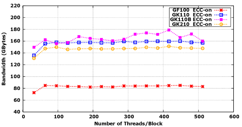
Figure 5: Performance of the propagate kernel (ECC enabled), on C2050 (GF100 GPU), K20X (GK110 GPU), K40 (GK110B GPU) systems and on one GPU of a K80 (GK210 GPU) board, vs. number of threads per block, on a lattice of $\approx 4$ million of cells.

The bc kernel enforces boundary conditions (constant temperature and zero velocity of the fluid) at the top and bottom of the lattice; it runs only on the threads corresponding to lattice sites with coordinate $y=0,1,2$ and $y=L_{y}-1,L_{y}-2,L_{y}-3$. The layout of each CUDA block is the same as for the propagate kernel, and the code uses if statements to disable threads not involved in the computation. This causes thread divergence, but, as we show later, the computational cost of the bc kernel is negligible compared to all other steps, so performance drops in this kernel have a minor global impact.

The collide Kernel

The collide kernel takes care of the collision of populations gathered by the propagate step. At each time step, each thread reads populations of each lattice site from the prv arrays, performs all needed mathematical operations and stores the resulting populations onto the nxt array. The roles of nxt and prv are swapped at each iteration. In this scheme, memory reads and writes are always sequential and properly aligned, enabling memory coalescing.

collide is a strongly compute bound routine. This is shown in Tab.  2, collecting the output of the NVIDIA nvprof execution profiler. After compilation and optimization the collide kernel executes $6472$ double-precision mathematical operations for each lattice site, but only $\approx 72\%$ are executed as more efficient Fused-Multiply-Add (FMA), slightly reducing the overall performance. Data from the table translate into an arithmetic intensity of $\approx 11$ Flops/byte; using this figure and the ALU utilization, the needed memory bandwidth is only one third of the peak available on the GPU. This confirms that the kernel is limited by arithmetic throughput, rather than memory bandwidth. The thread and block organization here is the same as for propagate, see again Figure 3 right, and the corresponding parameters should again be tuned for performance. There is tension between the gains arising from a large number of data points being processed together and the limited register space available to store the huge number of constants and intermediate results that need to be maintained inside the processor as different data blocks are processed in turn.

Table 2: Output of the NVIDIA nvprof profiler for collide on a lattice of $2048\times 1024$ sites. The table shows the number of ADD, MUL and FMA (fused Multiply-Add) operations, the total number of floating-point operations per site and the fraction of cycles in which the ALU is used (ALU Utilization).

FLOPS (Double Add)	704684032
FLOPS (Double Mul)	1530290176
FLOPS (Double FMA)	5629132825
FLOPS per site	6472
ALU Utilization	High (70%)

Going into more technical details, we use data prefetch to hide memory accesses and on Kepler all loops accessing the thread-private prefetch array have been unrolled via #pragma unroll. This allows the compiler to keep the elements of the prefetch array in registers exploiting the larger register file available on the Kepler GPUs. We experimentally searched for the best tradeoff between register spilling and device occupancy manually setting the maximum number of threads per block and the minimum number of blocks per SM. This can be done using the launch_bounds directive [26]; this handcrafted optimization step improves performances by $\approx 20\%$.

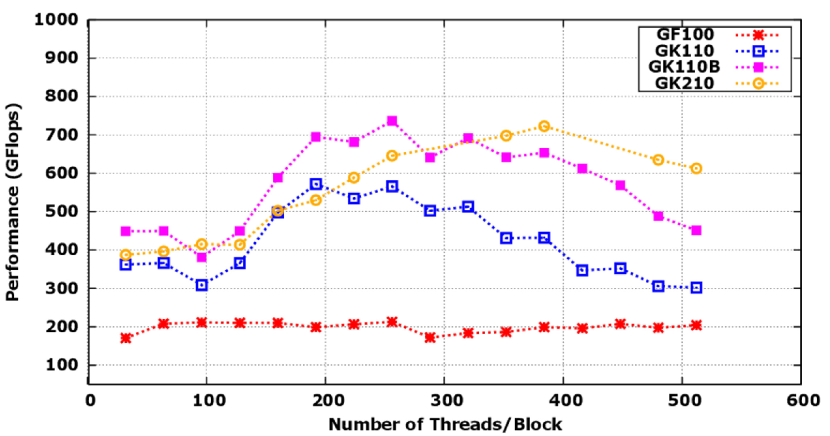
Figure 6: Performance of the collide kernel on C2050 (GF100), K20X (GK110), K40 (GK110B) systems and on one GPU of a K80 (GK210) board vs. the number of threads per block, on a lattice of $\approx 4$ million of cells.

Performance Analysis

Figure 6 shows the performance of the collide kernel as a function of the number of threads per block. On the C2050, it basically reaches a plateau for a number of threads larger than 64, and the sustained performance is $\approx 210$ GF/s, that is $\approx 40\%$ of peak. On the K20X and K40, the behavior is different: performance improves up to 256 threads per block reaching a peak value of $\approx 570$ GF/s for the K20X and $\approx 730$ GF/s for the K40, that is, respectively $\approx 43\%$ and $\approx 51\%$ of peak. Finally on one GPU of the K80 board, top performance is the same as the K40, but it is obtained with a larger value of threads per block, and performance decreases less sharply if this parameter is further increased.

As we try to use a larger number of threads, performance drops because the number of needed registers is larger than the available resources on the SMs. Indeed, as already remarked, the Kepler version of the collide kernel holds the values of the prefetch array in registers. Since the size of the register file is limited, more and more registers must be spilled to global memory if more threads per block are used. The L1 cache is too small to handle all spills and although the available device memory bandwidth for the spilling is not a bottleneck this has a negative impact on performance. The larger register file of the enhanced Kepler SMX on the Tesla K80 helps with that: this is why on this processor performance is more stable as the number of threads per block increases. In conclusion, the collide kernel is limited by memory latencies as the large amount of state per thread does not allow to run enough threads concurrently on the SMs to cover all latencies.

Further optimization steps are possible and have already been discussed in the literature, such as fusing the propagate and collide steps [14]; also, pbc can be overlapped with the execution of these steps, with some change in the scheduling of operations. The details of these optimizations depend significantly on how the lattice is split across processors in a multi-GPU implementations, so we defer this discussion to the next section.

5 Multi-GPU implementation

In this section we describe the structure and implementation of our code for a (large) multi-GPU cluster. We divide this section in three parts: we first discuss some simple theoretical model of performance that have guided our parallelization strategies; we then review the programming environment and tools available to support GPU-to-GPU communication, and finally present details of our implementation.

Modelling the impact of communications

A parallel multi-processor LBM code is in principle straightforward: one just maps regular tiles of the physical lattice on the processors; the processing load is balanced among processing elements if all domains have the same size; finally tile-to-tile communication patterns are regular and predictable and only involve (logically) nearest-neighbor processors. Still, node-to-node communications are an unavoidable overhead that may become serious, hampering performance scaling of the program, as the number of nodes increases. The amount of data to be moved is roughly proportional to the surface of each computational domain, while computing scales as the domain volume, so, in order to ensure better scaling figures, one should i) identify the domain decomposition that minimizes the surface-over-volume ratio and ii) overlap communications with parts of the computation that have no dependency with data incoming from neighbor nodes.

Simple performance models may guide actual program development. For a lattice with $N$ points in $D$ dimensions (i.e., with linear size $L=N^{1/D}$) one maps regular tiles onto $N_{p}$ processors; each tile contains points associated to all coordinate values in $D-d$ dimensions and an equal number of coordinate values in the remaining $d$ dimensions ($d\leq D$). One easily finds that the surface-over-volume ratio ($S/V$) is

$$S/V\simeq d~{}N_{p}^{1/d},$$ (11)

so in principle $d=D$ ($d=2$ in our case) should have the best scaling performance.

In practice, things are more complex for several reasons. One relevant point is that communications of data elements corresponding to borders in different directions may have widely different bandwidths. This depends on the data layout in memory, as this dictates which surface elements are stored at non-contiguous addresses, usually at fixed distance (stride) from each other. For memory-contiguous data words, a node-to-node communication involves a stream of data items from memory elements to the network interface, and then from the network interface again to contiguous memory cells. However data from sparse memory location has to be first gathered into a contiguous buffer, then transmitted and finally scattered to memory cells at sparse addresses. These access patterns may be much slower than for contiguous memory cells, so effective bandwidths may be widely different.

Consider a $2D$ lattice of $L_{x}\times L_{y}$ sites, that we partition on $N_{p}$ processing elements. Each processing element handles a tile of $(L_{x}/n_{x})\times(L_{y}/n_{y})$ sites ($n_{x}\times n_{y}=N_{p}$). Assume that transfers in the $X$ and $Y$ directions have effective (and in general different) bandwidths $B_{x}$ and $B_{y}$. The time needed to move information across all boundaries of each domain is proportional to $T_{C}$ (through a factor $S$ that counts how many bytes have to be moved for each boundary site):

$$T_{C}=\frac{L_{y}}{B_{y}n_{y}}+\frac{L_{x}}{B_{x}n_{x}},$$ (12)

We now ask what is the optimal choice for $n_{x}$ and $n_{y}$ corresponding to the minimum of Eq. 12, with $n_{x}\times n_{y}=N_{p}$. One easily finds that:

$$n_{x}=\sqrt{N_{p}}R,~{}~{}~{}~{}~{}~{}~{}n_{y}=\sqrt{N_{p}}/R$$ (13)

with $R=\sqrt{\frac{L_{x}B_{y}}{L_{y}B_{x}}}$ a factor taking into account the aspect-ratio of the lattice and the mismatch of the bandwidth values. Using these optimal choices, we further obtain:

$$T_{C}^{min}=\frac{2}{\sqrt{N_{p}}}\sqrt{\frac{L_{x}L_{y}}{B_{x}B_{y}}}.$$ (14)

Total processing time $T$ is the sum of communication time and (on-node) processing time $T_{P}$; the latter grows as the number of lattice sites handled by each processor, $T_{P}=\beta N/N_{p}$, so, $T=T_{P}+T_{C}$,

$$T=\beta\frac{N}{N_{p}}\{1+\frac{4S}{\beta}\frac{1}{\sqrt{B_{x}B_{y}}}\sqrt{N_{p}/N}\}$$ (15)

In this and in the following equations, we always write $T$ as a scaling term ($\beta N/N_{P}$) multiplied by a scale violating one (in braces). For comparison, if we tile the lattice in just one dimension (e.g., $Y$), a similar reasoning tells us that

$$T=\beta\frac{N}{N_{p}}\{1+\frac{2SL_{y}}{\beta B_{y}}N_{p}/N\}$$ (16)

which has obviously more severe asymptotic (large $N_{p}$) scaling violations.

It may be interesting to look at Eqs. 15 and 16 from the point of view of Brent’s theorem [27], that, in the framework of a PRAM model, states that

$$T\leq S_{N}+\frac{W_{N}-S_{N}}{N_{p}},$$ (17)

with $W_{N}$ the overall number of operations to be performed, and $S_{N}$ the longest path in the dependency graph of the algorithm. In our case, $W_{N}$ depends linearly on the lattice size, $W_{N}=w\times N$, with $w$ counting the number of operations to be performed on each lattice site, while $S_{N}$ is $N$ independent, $S_{N}=w$, since operations on different points of the lattice have no dependencies among them. In this case, Eq. 17 reads

$$T=w+\frac{w(N-1)}{N_{p}}=w(1+\frac{N-1}{N_{p}})\approx wN/N_{p};$$ (18)

our model (Eqs. 15 and 16) obtains the same result, apart from a correction due to communication overheads, that is not considered by Brent’s theorem since the PRAM model assumes shared-memory with uniform access time.

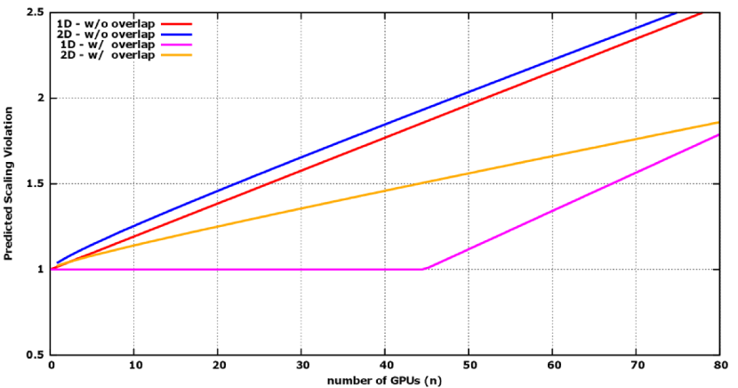
Figure 7: Scaling violations predicted by our performance model (Eqs. 15 to 20) on a lattice of $1940\times 1940$ sites, using experimentally measured single-node processing performance and node-to-node bandwidths for contiguous and non-contiguous data buffers. In 2D we use the possibly not-optimal choice $n_{x}=n_{y}$.

A further key observation is that, for each tile, all lattice points belonging to the bulk (i.e., away from the tile boundary by more than $3$ lattice points) have no dependency from data of other nodes. This suggests to overlap bulk processing and data transfer. For an 1-D tiling, the corresponding estimated processing times is

$$T=\beta\frac{N}{N_{p}}\{\max{(1-6L_{y}N_{p}/N,~{}\frac{2SL_{y}}{\beta B_{y}}N_{p}/N)}+6L_{y}N_{p}/N\}.$$ (19)

Going to 2-D tiling we need to gather not contiguous data in GPU memory for efficient node-to-node communication, which impacts overlap possibilities, or work with multiple small and less efficient node-to-node communication steps. Details of this will be explained in a later section. One is then forced to perform a communication step for non-contiguous data first (in the $Y$ direction in our case), followed by overlapped bulk computation and communication of contiguous buffers and finally by computation of border data. The corresponding estimate, that for simplicity we write only for square lattices and for the not necessarily optimal case $n_{x}=n_{y}=\sqrt{N_{p}}$, is:

$$T=\beta\frac{N}{N_{p}}\{\max{((1-12\sqrt{N_{p}/N}),~{}\frac{2S}{\beta B_{y}}\sqrt{N_{p}/N})}+\frac{2S}{\beta B_{x}}\sqrt{N_{p}/N}+12\sqrt{N_{p}/N}\}$$ (20)

Extracting accurate predictions from Eqs. 15 to 20 is made more difficult by the fact that communications bandwidths depend on the transfer direction (as already remarked) and also on buffer size. We have performed direct bandwidth measurements for relevant values of the buffer sizes (shown later, see Figure 12, where several important details of this measurement are discussed); putting those data into our model equations, we predict a pattern of scaling violations shown in Figure 7 for one typical lattice size. Several neglected factors may change the details of our predictions, so we stress again that we use our theoretical estimates for guidance only. Two main lessons emerge from our models: i) overlapping communication and computation has a strong impact on performance; if we do so to the extent made possible by system features, one can expect limited violations to scaling on reasonably-sized lattices and on a fairly large number of GPUs, and, ii) contrary to naive expectation, an 1-D tiling of the lattice may have good performances up to a reasonably large number of processors.

Based on this overall picture, we have prepared and tested several parallel versions of the code that we describe and compare in the following.

⬇

#ifdef MPI_REGULAR

cudaMemcpy ( sndbuf_h, sndbuf_d, N, cudaMemcpyDeviceToHost );

MPI_Sendrecv(

sndbuf_h, N, MPI_DATATYPE, nxt, 0,

rcvbuf_h, N, MPI_DATATYPE, prv, 0,

MPI_COMM_WORLD; MPI_STATUS_IGNORE );

cudaMemcpy ( rcvbuf_d, rcvbuf_h, N, cudaMemcpyHostToDevice );

#endif

#ifdef CUDA_AWARE_MPI

MPI_Sendrecv(

sndbuf_d, N, MPI_DATATYPE, nxt, 0,

rcvbuf_d, N, MPI_DATATYPE, prv, 0,

MPI_COMM_WORLD; MPI_STATUS_IGNORE );

#endif

Figure 8: Definition of two CUDA-codes for a bi-directional memory-copy of buffers allocated on two GPUs; the first case is a regular MPI implementation requiring to move explicitly data from GPU to host and vice-versa; the latter case uses CUDA-aware MPI allowing to call directly the MPI_Sendrecv with pointers to buffers in GPU memory as source and destination parameters.

Programming Models for Multi-GPU applications

In this sub-section we briefly overview programming models relevant for multi-GPU codes. The goal is to make code development and management easier and communications more efficient.

Large GPU clusters are widely heterogeneous computing systems: compute nodes have one or (usually) more CPUs; each CPU acts as host for a variable number of GPUs, ranging typically from 1 to 4; in the cluster that we have used for our tests each node has 2 CPUs and each CPU hosts 4 GPUs. GPUs are directly connected to their host through a PCIe interface, which has reasonably high bandwidth (several Gbytes/sec) but also long startup latency ($\geq 1\mu$sec). The network interface is also connected to one of the CPUs via PCIe. The complexity of this structure implies that what, at the application level, is a plain GPU-to-GPU communication may involve different routes, different communication strategies, and correspondingly different performances. We discuss here two key aspects of the problem, namely i) a programming environment able to specify in a unified way all different communication patterns and, ii) the ensemble of run-time support features that help maximize effective communication bandwidth for any possible pair of communication end-points.

Concerning the first point, a reasonable approach is to use the well known MPI communication libraries that currently also support GPUs; we then associate one MPI process to each GPU, so MPI libraries are able to automatically handle the transfer of data buffers from GPU to GPU in the most appropriate way. Transferred buffers must be allocated at contiguous locations on memory; however, transfers of non-contiguous buffers can also be handled automatically by MPI, using the derived vector data type: the vector data type describes how data buffers are placed in memory and the library automatically packs data into a contiguous buffer, perform the MPI communication and then unpack data at destination. Note that in regular MPI versions – i.e. without GPU support – these buffers had to be allocated on the host CPU, so each data transfer has to be preceded and followed by an explicit data move from/to GPU and its host. CUDA-aware MPI [28] improves on this, allowing to specify buffers allocated on the GPU memory as arguments of the MPI operations, making codes terser and more readable; Figure 8 compares the CUDA definitions of a function that performs a bi-directional remote memory-copy of a buffer allocated on the memory of two GPUs, using regular MPI and CUDA-aware MPI.

Armed with a clean way to specify the communication patterns needed by our program, we must now make sure that all possible steps are taken to reduce the latency of each communication, as this has a critical impact on the scaling performance of the complete code. This is done by enabling a variety of features, available in the low-level communication libraries; here we describe the most relevant points.

For GPUs attached to the same host-CPU, CUDA-IPC moves data directly across GPUs without staging on CPU-memory. This makes communication faster [17]. GPUs attached to different CPUs of the same node communicate through CPU-memory staging; here pipelining helps to shorten communication latency. For GPUs belonging to different nodes GPUDirect RDMA moves short data packets from the GPU to the network interface without any involvement of the host CPU. For longer data packets due to PCIe architectural bottlenecks, RDMA becomes less effective, see [29]. In this case, GPUDirect simplifies the operation by sharing a common staging region between the GPU and the network interface.

1-D Splitting

In this case, we divide a lattice of size $L_{x}\times L_{y}$ on $N_{p}$ GPUs tiling along just one dimension. In our case, since lattice is allocated by column-major order, we split the lattice along the $X$ dimension and then each GPU allocates a sub-lattice of size $L_{x}/N_{p}\times L_{y}$, see Figure 9.

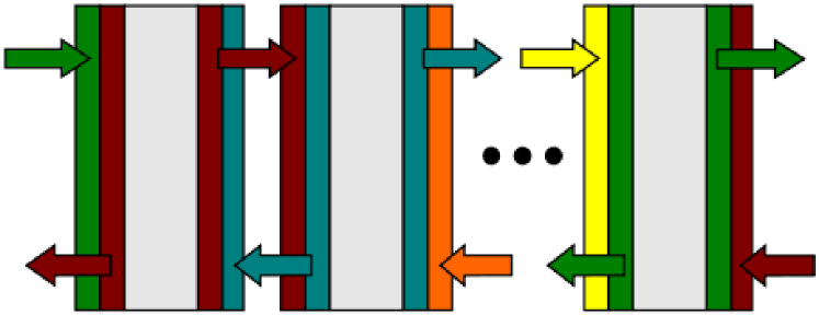
Figure 9: 1-D tiling of a lattice on $N_{p}$ GPUs virtually ordered along a ring.

This 1D tiling implies a virtual ordering of the GPUs along a ring, so each GPU is connected with a previous and a next GPU; at the beginning of each time-step, GPUs must exchange data, since cells close to the right and left edges of the sub-lattice of each GPU needs data allocated on the logically previous and next GPUs, see again Figure 9.

⬇

// Computing propagate over lattice bulk

prop_Bulk <<< dimGridB, dimBlockB, 0, stream[0] >>> ( … );

bc_Bulk <<< dimGridB, dimBlockB, 0, stream[0] >>> ( … );

collide_Bulk <<< dimGridB, dimBlockB, 0, stream[0] >>> ( … );

// Update halos

pbc_c();

// Computing propagate on left columns

prop_L <<< dimGridLR, dimBlockLR, 0, stream[1] >>> ( … );

collide_L <<< dimGridB, dimBlockB, 0, stream[1] >>> ( … );

// Computing propagate on right columns

prop_R <<< dimGridLR, dimBlockLR, 0, stream[2] >>> ( … );

collide_R <<< dimGridLR, dimBlockLR, 0, stream[2] >>> ( … );

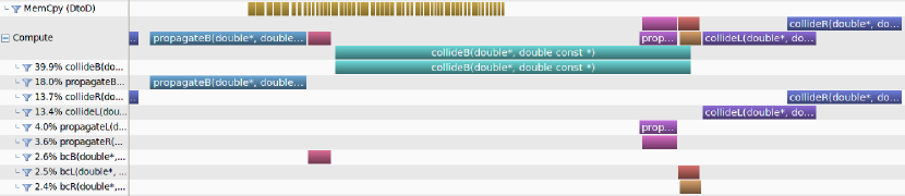
Figure 10: Sample code and timeline of a multi-GPU code executed by each MPI-process using the 1-d tiling of the lattice. Communications are performed by pbc and use CUDA-aware MPI; this step is then translated into CUDA device-to-device memory copies since this example refers to GPUs allocated on the same host; communication overlaps with the execution of the propagate, bc and collide kernels on the bulk of the lattice. After MPI communications have completed, the computational kernels acting on the right and left edges of the lattice can start; they do so as soon as GPU resources become available.

For processing, the lattice is divided in three regions: two regions of size $3\times Ly$ include the three leftmost and the three rightmost column-borders, while another region includes the central part of the lattice that we call the bulk. Processing the left and right regions can start only after the left and right halos have been updated, while processing on the bulk can start immediately and overlaps with the update of halos. Each MPI process executes a code structured as in Figure 10 top: it runs a CUDA-stream executing in sequence the propagate, bc and collide kernels on the bulk region. In parallel, the host-PC executes the pbc_c (_c stands for contiguous) function which performs MPI communications to update left and right halos with neighbor GPUs in the ring. After all data transfers are complete, two additional CUDA-streams start propagate, bc and collide on the left and right border regions.

Figure 10 bottom shows the timeline execution of the code. We directly see that an efficient implementation of pbc helps to enlarge the region in which linear scaling is possible; as we partition the lattice onto a larger and larger number of processors, the combined execution times of propagate, bc and collide reduces accordingly, while the execution time of pbc remains approximately constant. Eventually, pbc takes longer than the computational kernels, and scaling violations occur. There is no way to escape this situation asymptotically, but an efficient implementation of pbc_c delays the onset of scaling violations. We have found that the implementation of pbc_c through a sequence of CUDA-aware MPI operations gives good results; in our case, 26 populations must be moved for each boundary site, corresponding to 52 MPI operations. If the lattice is large enough in the Y direction ($\geq 512$ points) the overheads associated to separate MPI operations are negligible. For smaller lattices it may be useful to pack data in a contiguous buffer and perform just one larger MPI transfer. We discuss this further optimization in the next section, where we also consider the fusion of propagate and collide into just one CUDA kernel.

2D Splitting

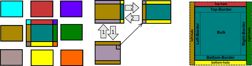
Figure 11: 2-D tiling of the lattice on $N_{p}$ GPUs. Left: diagram of the tiles and of the corresponding halos. Center: communication patterns to update halos belonging to a given tile. Righ: halo regions surrounding the tile.

Code organization using a 2-D tiling is slightly more complex. We split the lattice on a grid $n_{x}\times n_{y}$ GPUs, virtually arranged at the edges of a 2D mesh. Each GPU needs data allocated on eight neighbor GPUs, see Figure 11, left.

All needed data transfers (from adjacent and from diagonal neighbor nodes) can be done by performing a sequence (see again  Figure 11, center and right) in which first all nodes exchange data along one of the two directions, not including halo elements; when this is completed a further step in the orthogonal direction is started, including this time also halo elements.

One of the two communications steps (the one in the Y+ and Y- directions in our case) implies non-contiguous data elements. As discussed in an earlier section, communications of non contiguous buffers is automatically handled by MPI using the vector derived data type. The corresponding standard library gathers all data elements into an intermediate buffer, starts a transfer operation for the intermediate buffer and finally scatters received data items to their final destination. We tested two well-known CUDA-aware MPI libraries, OpenMPI and MVAPICH2. Results were unsatisfactory for two reasons: i) OpenMPI is affected by high overheads because of the many calls to copy all the pieces of data into the intermediate MPI buffer on the host; ii) MVAPICH2 do not use persistent intermediate MPI buffers, that are allocated and de-allocated on the GPU at each time step; the corresponding overhead in doing that is in our case too large, and it can be easily avoided using persistent allocation of communication buffers on GPU memory .

We have overcome these issues developing a custom communication library that uses persistent send and receive buffers, allocated once on the GPUs at program initialization. Every time a communication of non contiguous buffers is needed, function pbc_nc (_nc stands for non-contiguous) starts the pack kernel to gather non-contiguous data into a contiguous buffer allocated on the GPU. When this is done, an MPI communication is started, followed by a final scatter of the received data. Figure 20 in the appendix shows a simplified CUDA implementation of the pack and unpack kernels, and Figure 21 shows a sample code to handle data transfers among non contiguous buffers.

This strategy has the advantage that, for each halo update, only one MPI communication is needed. This avoids overheads associated to start MPI transfers, and keeps the size of MPI buffers large enough to minimize overheads caused by CUDA-IPC set-up. The advantages of this approach are relevant also for updating contiguous halos; for this reason we adopt it for communications in both directions.

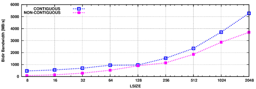
Figure 12: Measured effective bi-directional bandwidth to update contiguous and non contiguous halos as a function of the size of the lattice tile. The test has been done on two K80 systems on two remote nodes, interconnected by an Infiniband FDR network with GPUDirect RDMA enabled.

Figure 12 reflects the global result of this optimization effort, showing the effective bi-directional bandwidth measured in the update of memory-contiguous and non contiguous halos as a function of the corresponding lattice size. This test involves two K80 boards attached to two different host-CPUs interconnected through Infiniband network. We see that, as expected, non-contiguous halos have a reduced effective bandwidth, but the difference between the two cases is not too large. The data shown in Figure 12 has been used in the scaling prediction models that we have discussed before.

⬇

// Update non-contiguous halos

pbc_nc()

// Computing over bulk

prop_Bulk <<< .dimGridB, dimBlockB, 0, stream[0] >>> ( … )

collide_Bulk <<< dimGridB, dimBlockB, 0, stream[0] >>> ( … );

// Update contiguous halos

pbc_c()

// Computing propagate on left columns of the lattice

prop_L <<< dimGridLR, dimBlockLR, 0, stream[1] >>> ( … );

collide_L <<< dimGridLR, dimBlockLR, 0, stream[1] >>> ( … );

// Computing propagate on right columns of the lattice

prop_R <<< dimGridLR, dimBlockLR, 0, stream[2] >>> ( … );

collide_R <<< dimGridLR, dimBlockLR, 0, stream[2] >>> ( … );

// Computing propagate on top rows of the lattice

prop_T <<< dimGridTB, dimBlockTB, 0, stream[3] >>> ( … );

bc_T <<< dimGridTB, dimBlockTB, 0, stream[3] >>> ( … );

collide_T <<< dimGridTB, dimBlockTB, 0, stream[3] >>> ( … );

// Computing propagate on bottom rows of the lattice

prop_B <<< dimGridTB, dimBlockTB, 0, stream[4] >>> ( … );

bc_B <<< dimGridTB, dimBlockTB, 0, stream[4] >>> ( … );

collide_B <<< dimGridTB, dimBlockTB, 0, stream[4] >>> ( … );

Figure 13: Scheduling of operations for the code using 2-D tiles.

For the processing steps of the algorithm, the lattice is divided in five regions, see Figure11, right: two regions of $3Ly$ sites, including the three leftmost and the three rightmost columns, two regions of size $3L_{x}$ including the three topmost and lowermost rows and the central part of the lattice including all bulk sites. The code in Figure 13 shows how we schedule operations. We first exchange the (non-contiguous) top and bottom halos; when this operation has completed, we start processing the lattice bulk on a GPU stream, and in parallel we update the contiguous left and right halos. After all halos have been updated, we start separate GPU streams processing the left, right, top and bottom borders.

Figure 14: Execution timeline of the code using a 2-d tiling, as shown by the NVIDIA profiler. In this example, we first execute update of non-contiguous halos starting first the pack_bot kernel, and after MPI communication the unpack_tot. These operations can not overlap with other data-processing. After we start the pack_left and pack_right to pack data to update contiguous halos, and in parallel we execute the propagateCollideBulk kernel to process all sites belonging to lattice bulk. As soon as propagateCollideBulk kernel frees GPU resources, unpack_left and unpack_right kernels are executed to update contiguous halos, followed by the processing of the 4 border regions.

With this scheduling it is easy to merge propagate and collide for all points on which bc kernel does not apply, belonging to the bulk, left and right regions. On the other hand, top and bottom borders must be processed by a sequence of propagate, bc and collide kernels. Figure 22 shows the final organization of the code including these improvements, and Figure 14 shows the corresponding execution timeline as recorded by the NVIDIA profiler. The update of non-contiguous halos can not overlap (see caption for details) with other data-processing operation, because: i) MPI communications along Y direction needs to be done before starting that along the X direction to update also halos with data coming from diagonal neighbor sites, ii) and the corresponding pack and unpack kernels needs to be executed before GPU resources become busy in processing the sites of the lattice bulk. On the other hand, the update of contiguous halos fully overlaps with processing of the bulk region. Finally, unpack of received data for contiguous halos, and the processing of the 4 border regions starts as soon as GPU resources are freed by the kernel processing the bulk regions.

Table 3: Performance of our full production-ready code, measured on a lattice of $1024\times 8192$ sites. We show the execution time of each phase of the code, the performance of the propagate and collide kernels, the effective performance of the complete code (Global $P$), and the MLUPS (Million Lattice Updates per second) metric. The clock frequencies for the SMs of the K40 and K80 boards are set at the “boosted” values of $875$ MHz.

	GF100	2$\times$GF100	GK110B	2$\times$GK110B	GK210	2$\times$GK210
$T_{\mbox{prop}}$ (ms)	60.6	30.9	25.8	12.2	32.3	19.0
$T_{\mbox{bc}}$ (ms)	6.5	3.6	2.8	1.4	1.4	0.8
$T_{\mbox{coll}}$ (ms)	276.0	158.0	78.0	39.0	71.1	38.1
Propagate (GB/s)	81	155	187	376	155	261
Collide (GF/s)	197	344	696	1388	764	1544
Global $P$. (GF/s)	158	281	506	1010	519	988
MLUPS	24	43	78	156	80	153

6 Results Analysis

In this section we present results for our full production-grade codes, that consistently use all paths to performance discussed in the previous sections.

One GPU

We first examine results for just one (or two) GPUs: Table 3 collects performance results of the full production-ready code running on one host with one or two GPUs on a lattice of $1024\times 8192$ points; the main computational load is associated to the propagate and collide kernels, as expected. Memory bandwidth (relevant for propagate) is close to $55\%$ of the theoretical peak for the C2050 accelerator; it reaches $\approx 65\%$ of peak for the K40 and the K80. The Kepler processor is more efficient from the point of view of floating-point throughput, as measured by the FP performance of the collide kernel, reaching $\approx 43\%$ versus $\approx 38\%$ for the C2050 board; the K80 board exploits its larger register file and shared memory to reach $\approx 53\%$ of peak. On a dual-K40 system and on a K80 board using both GPUs, the collide kernel largely breaks the sustained double precision $1$ Tflops performance barrier; also the global performance figures of the full code, which take into account all execution phases, are satisfactory: we measure an efficiency of respectively $\approx 31\%$ and $\approx 34\%$ of the raw peak floating-point throughput.

Performance Comparison

It is interesting to compare the performance delivered by GPUs with that of other recent processors; this is done in Table 4, where we compare performance figures on GPUs systems with those of implementations of the same code developed and optimized for multi- and many-core Intel systems. We consider a dual-E5-2630 V3 system, with two eight-core Haswell V3 processors, and a 61-core Xeon-Phi processor, the latest accelerator based on the Intel MIC many-core architecture. For these architectures we have optimized the code parallelizing the execution over all available cores and using SIMD instructions within the cores; for details, see [30, 31] and [32, 33]. Performances of the propagate and collide kernels are significantly faster on the the K40 and K80 boards than on the other systems: the propagate kernel is approximately $2-3X$ faster than the dual-CPU systems, and $1.9X$ and $2.7X$ faster than the Xeon-Phi; this is also true for collide, where GPUs are $3.7X$ and $7.6X$ faster than CPUs, and $2.0X$ and $4.0X$ faster than the Xeon-Phi.

Energy Efficiency

Table 4 also shows data on energy efficiency (that we normalize to the average energy needed to process one lattice site). We estimate this quantity using published data on the Thermal Design Point (TDP), an upper bound of the power consumption of the processors; this gives only a rough estimate of the energy efficiency, also because all other sources of power consumption (host, memories, devices, …) are neglected. Taking these reservations into account, GPUs are more energy-efficient than the other processors: for instance, the K80 system is $\approx 7X$ better than the dual-CPU system and $\approx 4X$ better than the Xeon-Phi. When considering these results one must keep in mind that co-processors (GPUs and Xeon-Phi) operates with the support of a host processor: even if the latter is little used during the computation, it still draws an amount of power that is not necessarily a small fraction of the total energy budget.

Table 4: Performance comparison of the propagate and collide kernels running on several systems: a dual eight-core E5-2630 2.4 GHz (Intel Haswell V3) processor, an Intel Xeon-Phi accelerator and a K40 and K80 board. $\epsilon$ is the effective performance w.r.t. peak performance. For collide we also measure performance in Million Lattice Updates per Second (MLUPS). Finally we list the energy needed to update one lattice cell, estimating the power used by processors from published data on their Thermal Design Point (TDP).

	dual E5-2630 v3	Xeon-Phi 7120X	Tesla K40	Tesla K80
propagate (GB/s)	88	98	187	261
$\epsilon$	75%	28%	65%	54%
collide (GF/s)	222	362	696	1544
$\epsilon$	36%	30%	42%	53%
MLUPS	29	54	107	220
TDP (Watt)	2$\times$85	300	235	300
Energy ($\mu J$/site)	7.3	5.5	2.5	1.2

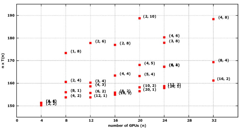
Figure 15: Benchmark results on a lattice of $3600\times 3600$ sites. For a varying number of GPUs ($n$) we plot (in arbitrary units) $n\times T(n)$ for all possible 1-D and 2-D decompositions of the lattice ( $T(n)$ is the wall-clock execution time); this product stays constant if the code enjoys perfect scalability.

Multi-GPU

We now move to consider scaling results for multi-GPU codes. Following our introductory discussion, we expect that – contrary to expectation – an 1D tiling of the lattice may be as efficient or even more efficient than a 2D tiling up to relatively large number of GPUs. We settle the question experimentally, measuring the performance of the codes described in the previous sections on several medium-size to large lattices, using all possible tilings consistent with the number of available GPUs. Our tests have been run on a GPU cluster installed at the NVIDIA Technology Center. Each node is a dual socket 10-core Ivy Bridge E5-2690 v2 at 3.00GHz, with 4 K80 GPUs. Nodes are interconnected with an Infiniband FDR network, and up to 32 GPUs are available.

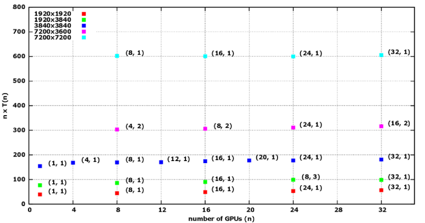
Figure 16: Measured values (in arbitrary units) of $n\times T(n)$ for the more efficient decomposition of the lattice, for several lattice sizes and for several numbers of GPUs ($n$); this product stays constant if the code enjoys perfect scalability.

Figure 15 presents a sample subset of our results, plotting $n\times T(n)$ (in arbitrary units) on a lattice of $3600\times 3600$ points for almost all possible 1-D and 2-D tilings of the lattice on $n$ GPUs. This quantity is constant if the program enjoys perfect scaling, so it is a direct measurement of scaling violations. Scaling violations are less than 10% up to 32 GPUs, and some tiling choices are clearly more efficient then others; as predicted by our model, the 1D tiling enjoys good scaling up to a reasonably large (24 in this case) number of GPUs. From this data (and from equivalent data for other lattice sizes) and for each value of $n$, we derive the best tiling choice; this is shown in Figure 16, that contains results for all lattice sizes that we have considered. We see here that scaling violations are relatively small (and of course smaller for larger lattices) on all lattices and for all $n$ that we have tested.

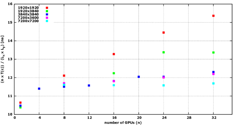
Figure 17: Measured values (in nsec) of the average time needed by one GPU to process one lattice site as a function of the number of GPUs ($n$), for the more efficient decomposition of the lattice and for several lattice sizes.

Figure 17 shows equivalent information, possibly in a more useful format: we consider again all lattices showing $T_{s}$, the time (in nsec) required to handle one lattice point by one GPU: we see an abrupt (and expected) transition as we move from 1 GPU to more GPUs, then a large plateau for large lattices and gentle scaling violations for the smaller lattices.

For physics users, the ultimate metric is the relative speed up and the effective performance as a function of $n$; this is shown in Figure 18, that wraps up our results.

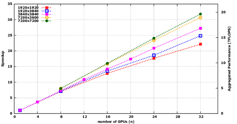
Figure 18: Aggregate performance of the code for the best lattice tiling as a function of the number of GPUs, for several lattice sizes. Results are shown as speedup values (left) or effective sustained performance (Tflops, right).

Performance increases smoothly for all lattices and number of GPUs: performance is not ideal but the bottom line of this analysis is that our codes run efficiently on up to at least 32 GPUs for physics relevant lattice sizes, with a sustained performance in the range of tens of Tflops.

Overview of Physics Results

We finally mention that the codes described in this paper have been used to perform extensive studies of thermally-driven turbulence in 2D systems. In Figure 19 we show the temperature maps of a simulation of the Rayleigh-Taylor instability at several stages during time evolution. This picture refers to a sample lattice of $2048\times 4096$ cells. Detailed physics results are in [34, 35, 36].

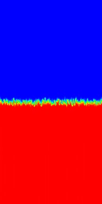
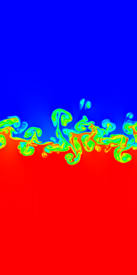
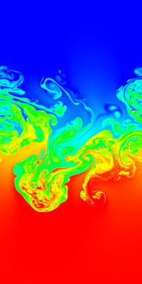
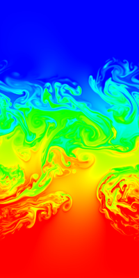
Figure 19: Temperature maps (red: highest temperature, blue: lowest temperature) of a simulation of a Rayleigh-Taylor instability on a lattice of $2048\times 4096$ cells at several stages of its time evolution.

7 Conclusions and Outlook

This paper presents a detailed account of the development and optimization of a production-grade Lattice Boltzmann code on two recent generations of GPUs. The strategies we have adopted are based on a quantitative approach that uses specific benchmarks and simple theoretical models as a guide to efficient implementation choices. We believe that the methodology that has guided our main design decisions can be helpful to develop GPU codes for other scientific applications.

We have obtained excellent sustained performance. This result admittedly builds on a carefully handcrafted adjustment of key kernels in the code, that takes into account the architecture of the target processor; however the effort of writing the corresponding CUDA-C code remains within reasonable limits.

Our results build on the excellent floating point performance of GPUs and on the capability of the memory-interface to support a large fraction of the peak bandwidth if one pays appropriate attention to the memory access patterns.

When going to a large multi-GPU implementation, node-to-node communication quickly become a serious bottleneck, so an optimization effort is needed both at the level of the algorithm and of the communication tools; algorithmic optimizations strictly depend on the application, while for the second point the CUDA-aware supports available on MPI libraries has significant benefits.

For problem sizes relevant for physics, fairly large systems (e.g. 32 GPUs) have very good strong scaling results, and the aggregated performance is not too far from $\approx 20$ Tflops.

Take-away lessons, applicable to different applications and beyond the obvious fact that as much parallelism as possible must be exposed, are:

1. performance depends sharply on the number of used threads; this has a big impact on the computing structure of the code which, in the case of GPUs, must have a high level of data vectorization;

2. good data allocation strategies help the memory controller coalesce memory requests; for GPUs the SoA scheme is preferred; this may require a complete or partial rewriting of existing applications since many codes use the AoS scheme which better fits the cache structure of traditional CPUs;

3. data transfers in and out of the accelerator must be minimized and overlapped with computation. Currently this is a serious limit to strong scalability for applications running on GPU clusters. CUDA-aware MPI library implementations, enabling specific GPU supports (CUDA-IPC and GPUDirect RDMA) provide significant advantages.

A number of programming frameworks have been introduced recently, with the aim to help programmers to write “portable” codes. Some of these like OpenCL use a language approach like CUDA, but they target a wider range of accelerator architectures. Other frameworks, e.g., OpenMP4 and OpenACC, use directives, allowing programmers to annotate regions of codes where parallelism can be exploited, so they can be automatically mapped and optimized by a compiler for several target parallel architectures. These environments are still immature in some respects: i) they do not reach yet the same level of performance as codes written using specific languages for the target accelerator, or ii) they support efficiently just a limited subset of architectures, leaving the portability issues partially solved. We are currently investigating the advantages of these frameworks for LBM code developments; for preliminary results see [37, 38, 39, 40, 41].

Appendix A Code Listings

⬇

// Pack non-contiguous buffer in a contiguous buffer

__global__ void pack(data_t *f, data_t *sndBuf){

int idx_c, idx_nc;

idx_c = ( blockIdx.y * blockDim.y * blockDim.x ) +

( threadIdx.y * blockDim.x ) +

( threadIdx.x );

idx_nc = ( blockIdx.y * blockDim.y * NY ) +

( threadIdx.y * NY ) +

( threadIdx.x );

if( threadIdx.x < blockDim.x )

sndBuf[ idx_c ] = f[ idx_nc ];

}

// Unpack a contiguous buffer in a non-contiguous buffer

__global__ void unpack(data_t *rcvBuf, data_t *f){

int idx_c, idx_nc;

idx_c = ( blockIdx.y * blockDim.y * blockDim.x ) +

( threadIdx.y * blockDim.x ) +

( threadIdx.x );

idx_nc = ( blockIdx.y * blockDim.y * NY ) +

( threadIdx.y * NY ) +

( threadIdx.x );

if( threadIdx.x < blockDim.x )

f[ idx_nc ] = rcvBuf[ idx_c ];

}

Figure 20: CUDA implementation of the pack and unpack kernels. pack starts a CUDA grid, and each thread reads a data item from a lattice site and stores it into an array at consecutive address. unpack does the opposite.

⬇

// send/receive buffer allocation

cudaMalloc((void **) &sndTopBuf, LY*HX*sizeof(data_t));

cudaMalloc((void **) &rcvBotBuf, LY*HX*sizeof(data_t));

cudaMalloc((void **) &sndBotBuf, LY*HX*sizeof(data_t));

cudaMalloc((void **) &rcvTopBuf, LY*HX*sizeof(data_t));

// function to transfer non-contiguous borders

void pbc_nc() {

// Pack top non-contiguous border

pack <<<dimGrid, dimBlock>>> (src_p, sndTopBuf);

// Wait the end of pack-kernel

cudaDeviceSynchronize();

// Exchange the contiguous buffer using CUDA-aware MPI

MPI_Sendrecv(

sndTopBuf, LY*HX, MPI_DOUBLE, mpi_left, 0,

rcvBotBuf, LY*HX, MPI_DOUBLE, mpi_right, 0,

MPI_COMM_WORLD, MPI_STATUS_IGNORE

);

// Unpack data on bottom halo

unpack <<< dimGrid, dimBlock >>> (rcvBotBuf, dst_p);

// Pack bottom non-contiguous border

pack <<<dimGrid, dimBlock>>> (src_p, sndBotBuf);

// Wait the end of pack-kernel

cudaDeviceSynchronize();

// Exchange the contiguous buffer using CUDA-aware MPI

MPI_Sendrecv(

sndBotBuf, LY*HX, MPI_DOUBLE, mpi_left, 0,

rcvTopBuf, LY*HX, MPI_DOUBLE, mpi_right, 0,

MPI_COMM_WORLD, MPI_STATUS_IGNORE

);

// Unpack data on bottom halo

unpack <<< dimGrid, dimBlock >>> (rcvTopBuf, dst_p);

// Wait end of unpack kernel

cudaDeviceSynchronize();

}

Figure 21: Sample code to handle data transfers among non contiguous buffers. Two buffers sndBuf and rcvBuf are persistently allocated on the GPU. Function pbc_nc performs the transfers of the data associated to the left and right halos. Real code we use is more complex because we overlaps the two transfers as much as possible running pack and unpack kernels on separate streams, and using asynchronous MPI operations. Execution of this function has to be completed before starting operations on lattice bulk and update of contiguous halos to ensure that halos are correctly updated.

⬇

// update non-contiguous halos

pbc_nc( f2_soa_d );

// pack right/left borders

pack_right <<< …, stream[1] >>> ( … );

pack_left <<< …, stream[2] >>> ( … );

// run propagateAndCollide over Bulk

propagateCollideBulk <<< …, stream[0] >>> ( … );

// wait end of pack right borders

cudaStreamSynchronize(stream[1]);

// perform MPI operations

MPI_Sendrecv( );

// wait end of pack left borders

cudaStreamSynchronize(stream[2]);

MPI_Sendrecv( );

// unpack right/left halos

unpack_left <<< …, stream[1] >>> ( … );

unpack_right <<< …, stream[2] >>> ( … );

// wait end of unpack right/left halos

// (required before starting processing left, right, top and bottom borders)

cudaStreamSynchronize(stream[1]);

cudaStreamSynchronize(stream[2]);

// process left/right borders

propagateCollideL <<< …, stream[1] >>> ( … );

propagateCollideR <<< …, stream[2] >>> ( … );

// process top/bottom borders

if (uppermost-rank){

propagateT <<< …, stream[3] >>> ( … );

bcT <<< …, stream[3] >>> ( … );

collideT <<< …, stream[3] >>> ( … );

} else {

propagateCollideT <<< …, stream[3] >>> ( … );

}

if (lowermost-rank){

propagateB <<< …, stream[4] >>> ( … );

bcB <<< …, stream[4] >>> ( … );

collideB <<< …, stream[4] >>> ( … );

} else {

propagateCollideB <<< …, stream[4] >>> ( … );

}

cudaDeviceSynchronize();

Figure 22: Overall organization of the code for a 2-D tiling of the lattice, fusing the propagate and collide kernels in one step. The code first update non contiguous halos calling function pbc_nc explained in Figure 21. After this is fully completed, starts pack of left and right borders on two GPU streams, and in parallel starts execution of propagateCollideBulk kernel processing lattice bulk. As MPI operations complete, data are unpacked on left and right halos, and we start processing of left, right, top and bottom borders. For left and right borders, we apply kernels propagateCollideL and propagateCollideR computing propagate and collide phases in one step. For top and bottom borders, we apply in sequence propgate, bc and collide kernels is the GPU is associated to a tile at top and bottom region of the lattice. Otherwise we only run propagateCollideT and propagateCollideB.

References

- [1] N. Maruyama, T. Aoki, Optimizing stencil computations for nvidia kepler gpus, in: International Workshop on High-Performance Stencil Computations, 2014, pp. 1–7.
- [2] A. Vizitiu, L. Itu, L. Lazar, C. Suciu, Double precision stencil computations on kepler gpus, in: System Theory, Control and Computing (ICSTCC), 2014 18th International Conference, 2014, pp. 123–127. doi:10.1109/ICSTCC.2014.6982402.
- [3] J. Holewinski, L.-N. Pouchet, P. Sadayappan, High-performance code generation for stencil computations on gpu architectures, in: Proceedings of the 26th ACM International Conference on Supercomputing, ICS ’12, ACM, New York, NY, USA, 2012, pp. 311–320. doi:10.1145/2304576.2304619.
- [4] A. Vizitiu, L. Itu, C. Niţă, C. Suciu, Optimized three-dimensional stencil computation on fermi and kepler gpus, in: High Performance Extreme Computing Conference (HPEC), 2014 IEEE, 2014, pp. 1–6. doi:10.1109/HPEC.2014.7040968.
- [5] C. Bonati, G. Cossu, M. D’Elia, P. Incardona, QCD simulations with staggered fermions on GPUs, Computer Physics Communications 183 (4) (2012) 853–863. doi:10.1016/j.cpc.2011.12.011.
- [6] M. A. Clark, R. Babich, K. Barros, R. C. Brower, C. Rebbi, Solving Lattice QCD systems of equations using mixed precision solvers on GPUs, Comput. Phys. Commun. 181 (2010) 1517–1528. doi:10.1016/j.cpc.2010.05.002.
- [7] J. Tölke, Implementation of a lattice boltzmann kernel using the compute unified device architecture developed by nvidia, Computing and Visualization in Science 13 (1) (2008) 29–39. doi:10.1007/s00791-008-0120-2.
- [8] M. Bernaschi, M. Fatica, S. Melchionna, S. Succi, E. Kaxiras, A flexible high-performance lattice boltzmann gpu code for the simulations of fluid flows in complex geometries, Concurrency and Computation: Practice and Experience 22 (1) (2010) 1–14. doi:10.1002/cpe.1466.
- [9] P. Ripesi, L. Biferale, S. F. Schifano, R. Tripiccione, Evolution of a double-front rayleigh-taylor system using a graphics-processing-unit-based high-resolution thermal lattice-boltzmann model, Physical Review E - Statistical, Nonlinear, and Soft Matter Physics 89 (4). doi:10.1103/PhysRevE.89.043022.
- [10] L. Biferale, F. Mantovani, M. Pivanti, M. Sbragaglia, A. Scagliarini, S. F. Schifano, F. Toschi, R. Tripiccione, Lattice Boltzmann fluid-dynamics on the QPACE supercomputer, Procedia Computer Science 1 (1) (2010) 1075–1082, ICCS 2010. doi:10.1016/j.procs.2010.04.119.
- [11] L. Biferale, F. Mantovani, M. Pivanti, F. Pozzati, M. Sbragaglia, A. Scagliarini, S. F. Schifano, F. Toschi, R. Tripiccione, A multi-gpu implementation of a d2q37 lattice boltzmann code, in: R. Wyrzykowski, J. Dongarra, K. Karczewski, J. Waśniewski (Eds.), Parallel Processing and Applied Mathematics: 9th International Conference, PPAM 2011, Torun, Poland, September 11-14, 2011. Revised Selected Papers, Part I, Lecture Notes in Computer Science, Springer Berlin Heidelberg, Berlin, Heidelberg, 2012, pp. 640–650. doi:10.1007/978-3-642-31464-3\_65.
- [12] G. Wellein, T. Zeiser, G. Hager, S. Donath, On the single processor performance of simple lattice Boltzmann kernels, Computers & Fluids 35 (8–9) (2006) 910–919, proceedings of the First International Conference for Mesoscopic Methods in Engineering and Science. doi:10.1016/j.compfluid.2005.02.008.
- [13] T. Pohl, M. Kowarschik, J. Wilke, K. Iglberger, U. Rüde, Optimization and profiling of the cache performance of parallel lattice boltzmann codes, Parallel Processing Letters 13 (04) (2003) 549–560. doi:10.1142/S0129626403001501.
- [14] M. Wittmann, T. Zeiser, G. Hager, G. Wellein, Comparison of different propagation steps for the lattice boltzmann method, CoRR abs/1111.0922.
- [15] A. G. Shet, S. H. Sorathiya, S. Krithivasan, A. M. Deshpande, B. Kaul, S. D. Sherlekar, S. Ansumali, Data structure and movement for lattice-based simulations, Phys. Rev. E 88 (2013) 013314. doi:10.1103/PhysRevE.88.013314.
- [16] A. G. Shet, K. Siddharth, S. H. Sorathiya, A. M. Deshpande, S. D. Sherlekar, B. Kaul, S. Ansumali, On vectorization for lattice based simulations, International Journal of Modern Physics C 24. doi:10.1142/S0129183113400111.
- [17] J. Kraus, M. Pivanti, S. F. Schifano, R. Tripiccione, M. Zanella, Benchmarking GPUs with a parallel Lattice-Boltzmann code, in: Computer Architecture and High Performance Computing (SBAC-PAD), 25th International Symposium on, IEEE, 2013, pp. 160–167. doi:10.1109/SBAC-PAD.2013.37.
- [18] L. Biferale, F. Mantovani, M. Pivanti, F. Pozzati, M. Sbragaglia, A. Scagliarini, S. F. Schifano, F. Toschi, R. Tripiccione, Optimization of Multi-Phase Compressible Lattice Boltzmann Codes on Massively Parallel Multi-Core Systems, Procedia Computer Science 4 (2011) 994–1003, proceedings of the International Conference on Computational Science, ICCS 2011. doi:10.1016/j.procs.2011.04.105.
- [19] L. Biferale, F. Mantovani, M. Pivanti, F. Pozzati, M. Sbragaglia, A. Scagliarini, S. F. Schifano, F. Toschi, R. Tripiccione, An optimized d2q37 lattice boltzmann code on gp-gpus, Computers & Fluids 80 (2013) 55 – 62. doi:10.1016/j.compfluid.2012.06.003.
- [20] M. Pivanti, F. Mantovani, S. F. Schifano, R. Tripiccione, L. Zenesini, An optimized lattice boltzmann code for BlueGene/Q, in: R. Wyrzykowski, J. Dongarra, K. Karczewski, J. Waśniewski (Eds.), Parallel Processing and Applied Mathematics: 10th International Conference, PPAM 2013, Warsaw, Poland, September 8-11, 2013, Revised Selected Papers, Part II, Lecture Notes in Computer Science, Springer Berlin Heidelberg, Berlin, Heidelberg, 2014, pp. 385–394. doi:10.1007/978-3-642-55195-6\_36.
- [21] S. Succi, The Lattice-Boltzmann Equation, Oxford university press, Oxford, 2001.
- [22] M. Sbragaglia, R. Benzi, L. Biferale, H. Chen, X. Shan, S. Succi, Lattice Boltzmann method with self-consistent thermo-hydrodynamic equilibria, Journal of Fluid Mechanics 628 (2009) 299–309. doi:10.1017/S002211200900665X.
- [23] A. Scagliarini, L. Biferale, M. Sbragaglia, K. Sugiyama, F. Toschi, Lattice Boltzmann methods for thermal flows: Continuum limit and applications to compressible Rayleigh–Taylor systems, Physics of Fluids (1994-present) 22 (5) (2010) 055101. doi:10.1063/1.3392774.
-
[24]
Nvidia,
fermi.
URL http://www.nvidia.com/content/PDF/fermi_white_papers/NVIDIA_Fermi_Compute_Architecture_Whitepaper.pdf -
[25]
Nvidia,
kepler gk110.
URL http://www.nvidia.com/content/PDF/kepler/NVIDIA-Kepler-GK110-Architecture-Whitepaper.pdf -
[26]
Nvidia cuda c
programming guide.
URL http://docs.nvidia.com/cuda/cuda-c-programming-guide - [27] R. P. Brent, The parallel evaluation of general arithmetic expressions, J. ACM 21 (2) (1974) 201–206. doi:10.1145/321812.321815.
-
[28]
An
introduction to cuda-aware mpi.
URL http://developer.nvidia.com/content/introduction-cuda-aware-mpi -
[29]
Benchmarking
gpudirect rdma on modern server platforms.
URL http://devblogs.nvidia.com/parallelforall/benchmarking-gpudirect-rdma-on-modern-server-platforms - [30] F. Mantovani, M. Pivanti, S. F. Schifano, R. Tripiccione, Performance issues on many-core processors: A d2q37 lattice boltzmann scheme as a test-case, Computers & Fluids 88 (2013) 743 – 752. doi:10.1016/j.compfluid.2013.05.014.
- [31] F. Mantovani, M. Pivanti, S. F. Schifano, R. Tripiccione, Exploiting parallelism in many-core architectures: Lattice boltzmann models as a test case, Journal of Physics: Conference Series 454 (1). doi:10.1088/1742-6596/454/1/012015.
- [32] G. Crimi, F. Mantovani, M. Pivanti, S. F. Schifano, R. Tripiccione, Early Experience on Porting and Running a Lattice Boltzmann Code on the Xeon-phi Co-Processor, Procedia Computer Science 18 (2013) 551–560. doi:10.1016/j.procs.2013.05.219.
- [33] G. Bortolotti, M. Caberletti, G. Crimi, A. Ferraro, F. Giacomini, M. Manzali, G. Maron, M. Pivanti, D. Salomoni, S. F. Schifano, R. Tripiccione, M. Zanella, Computing on knights and kepler architectures, Journal of Physics: Conference Series 513 (5) (2014) 052032.
- [34] L. Biferale, F. Mantovani, M. Sbragaglia, A. Scagliarini, F. Toschi, R. Tripiccione, Second-order closure in stratified turbulence: Simulations and modeling of bulk and entrainment regions, Physical Review E 84 (1) (2011) 016305. doi:10.1103/PhysRevE.84.016305.
- [35] L. Biferale, F. Mantovani, M. Sbragaglia, A. Scagliarini, F. Toschi, R. Tripiccione, Reactive Rayleigh-Taylor systems: Front propagation and non-stationarity, EPL 94 (5) (2011) 54004. doi:10.1209/0295-5075/94/54004.
- [36] A. Scagliarini, L. Biferale, F. Mantovani, M. Pivanti, F. Pozzati, M. Sbragaglia, S. F. Schifano, F. Toschi, R. Tripiccione, Front propagation in Rayleigh-Taylor systems with reaction, in: Journal of Physics: Conference Series, Vol. 318, IOP Publishing, 2011, pp. 1–10. doi:10.1088/1742-6596/318/9/092024.
- [37] E. Calore, S. F. Schifano, R. Tripiccione, A Portable OpenCL Lattice Boltzmann Code for Multi-and Many-core Processor Architectures, Procedia Computer Science 29 (2014) 40–49. doi:10.1016/j.procs.2014.05.004.
- [38] E. Calore, S. F. Schifano, R. Tripiccione, On portability, performance and scalability of an mpi opencl lattice boltzmann code, in: L. Lopes, J. Žilinskas, A. Costan, R. G. Cascella, G. Kecskemeti, E. Jeannot, M. Cannataro, L. Ricci, S. Benkner, S. Petit, V. Scarano, J. Gracia, S. Hunold, S. L. Scott, S. Lankes, C. Lengauer, J. Carretero, J. Breitbart, M. Alexander (Eds.), Euro-Par 2014: Parallel Processing Workshops: Euro-Par 2014 International Workshops, Porto, Portugal, August 25-26, 2014, Revised Selected Papers, Part II, Lecture Notes in Computer Science, Springer International Publishing, Cham, 2014, pp. 438–449. doi:10.1007/978-3-319-14313-2\_37.
- [39] E. Calore, J. Kraus, S. F. Schifano, R. Tripiccione, Accelerating lattice boltzmann applications with openacc, in: L. J. Träff, S. Hunold, F. Versaci (Eds.), Euro-Par 2015: Parallel Processing: 21st International Conference on Parallel and Distributed Computing, Vienna, Austria, August 24-28, 2015, Proceedings, Lecture Notes in Computer Science, Springer Berlin Heidelberg, Berlin, Heidelberg, 2015, pp. 613–624. doi:10.1007/978-3-662-48096-0\_47.
- [40] J. Kraus, M. Schlottke, A. Adinetz, D. Pleiter, Accelerating a c++ cfd code with openacc, in: Accelerator Programming using Directives (WACCPD), 2014 First Workshop on, 2014, pp. 47–54. doi:10.1109/WACCPD.2014.11.
- [41] E. Calore, A. Gabbana, J. Kraus, S. F. Schifano, R. Tripiccione, Performance and portability of accelerated lattice boltzmann applications with openacc, Concurrency and Computation: Practice and Experiencedoi:10.1002/cpe.3862.