Incremental computation of block triangular matrix exponentials with application to option pricing

Abstract

We study the problem of computing the matrix exponential of a block triangular matrix in a peculiar way: Block column by block column, from left to right. The need for such an evaluation scheme arises naturally in the context of option pricing in polynomial diffusion models. In this setting a discretization process produces a sequence of nested block triangular matrices, and their exponentials are to be computed at each stage, until a dynamically evaluated criterion allows to stop. Our algorithm is based on scaling and squaring. By carefully reusing certain intermediate quantities from one step to the next, we can efficiently compute such a sequence of matrix exponentials.

Key words

Matrix exponential, block triangular matrix, polynomial diffusion models, option pricing

1 Introduction

We study the problem of computing the matrix exponential for a sequence of nested block triangular matrices. In order to give a precise problem formulation, consider a sequence of block upper triangular matrices $G_{0},G_{1},G_{2},\dotsc$ of the form

$$G_{n}=\begin{bmatrix}G_{0,0}&G_{0,1}&\cdots&G_{0,n}\\ &G_{1,1}&\cdots&G_{1,n}\\ &&\ddots&\vdots\\ &&&G_{n,n}\\ \end{bmatrix}\in{\mathbb{R}}^{d_{n}\times d_{n}},$$ (1)

where all diagonal blocks $G_{n,n}$ are square. In other words, the matrix $G_{i}$ arises from $G_{i-1}$ by appending a block column (and adjusting the size). We aim at computing the sequence of matrix exponentials

$$\exp(G_{0}),\;\exp(G_{1}),\;\exp(G_{2}),\;\dotsc.$$ (2)

One could, of course, simply compute each of the exponentials (2) individually using standard techniques (see [11] for an overview). However, the sequence of matrix exponentials (2) inherits the nested structure from the matrices $G_{n}$ in (1), i.e., $\exp(G_{n-1})$ is a leading principle submatrix of $\exp(G_{n})$. In effect only the last block column of $\exp(G_{n})$ needs to be computed and the goal of this paper is to explain how this can be achieved in a numerically safe manner.

In the special case where the spectra of the diagonal blocks $G_{n,n}$ are separated, Parlett’s method [13] yields – in principle – an efficient computational scheme: Compute $F_{0,0}\mathrel{\mathop{:}}=\exp(G_{0,0})$ and $F_{1,1}\mathrel{\mathop{:}}=\exp(G_{1,1})$ separately, then the missing (1,2) block of $\exp(G_{1})$ is given as the unique solution $X$ to the Sylvester equation

$$G_{0,0}X-XG_{1,1}=F_{0,0}G_{0,1}-G_{0,1}F_{1,1}.$$

Continuing in this manner all the off-diagonal blocks required to compute (2) could be obtained from solving Sylvester equations. However, it is well known (see chapter 9 in [8]) that Parlett’s method is numerically safe only when the spectra of the diagonal blocks are well separated, in the sense that all involved Sylvester equations are well conditioned. Since we consider the block structure as fixed, imposing such a condition would severely limit the scope of applications; it is certainly not met by the application we discuss below.

A general class of applications for the described incremental computation of exponentials arises from the matrix representations of a linear operator $\mathcal{G}:V\to V$ restricted to a sequence of nested, finite dimensional subspaces of a given infinite dimensional vector space $V$. More precisely, one starts with a finite dimensional subspace $V_{0}$ of $V$ with a basis $\mathcal{B}_{0}$. Successively, the vector space $V_{0}$ is extended to $V_{1}\subseteq V_{2}\subseteq\cdots\subseteq V$ by generating a sequence of nested bases $\mathcal{B}_{0}\subseteq\mathcal{B}_{1}\subseteq\mathcal{B}_{2}\subseteq\cdots$. Assume that $\mathcal{G}V_{n}\subseteq V_{n}$ for all $n=0,1,\dotsc$, and consider the sequence of matrix representations $G_{n}$ of $\mathcal{G}$ with respect to $\mathcal{B}_{n}$. Due to the nestedness of the bases, $G_{n}$ is constructed from $G_{n-1}$ by adding the columns representing the action of $\mathcal{G}$ to $\mathcal{B}_{n}\setminus\mathcal{B}_{n-1}$. As a result, we obtain a sequence of matrices structured as in (1).

A specific example for the scenario outlined above arises in computational finance, when pricing options based on polynomial diffusion models; see [6]. As we explain in more detail in section 3, in this setting $\mathcal{G}$ is the generator of a stochastic differential equation (SDE), and $V_{n}$ are nested subspaces of multivariate polynomials. Some pricing techniques require the computation of certain conditional moments that can be extracted from the matrix exponentials (2). While increasing $n$ allows for a better approximation of the option price, the value of $n$ required to attain a desired accuracy is usually not known a priori. Algorithms that choose $n$ adaptively can be expected to rely on the incremental computation of the whole sequence (2).

Exponentials of block triangular matrices have also been studied in other contexts. For two-by-two block triangular matrices, Dieci and Papini study conditioning issues in [4], and a discussion on the choice of scaling parameters for using Padé approximants to exponential function in [3]. In the case where the matrix is also block-Toeplitz, a fast exponentiation algorithm is developed in [2].

The rest of this paper is organized as follows. In section 2 we give a detailed description of our algorithm for incrementally computing exponentials of block triangular matrices as in (1). In section 3 we discuss polynomial diffusion models, and some pricing techniques which necessitate the use of such an incremental algorithm. Finally, numerical results are presented in section 4.

2 Incremental scaling and squaring

Since the set of conformally partitioned block triangular matrices forms an algebra, and $\exp(G_{n})$ is a polynomial in $G_{n}$, the matrix $\exp(G_{n})$ has the same block upper triangular structure as $G_{n}$, that is,

$$\exp(G_{n})=\begin{bmatrix}\exp(G_{0,0})&\ast&\cdots&\ast\\ &\exp(G_{1,1})&\ddots&\vdots\\ &&\ddots&\ast\\ &&&\exp(G_{n,n})\\ \end{bmatrix}\in{\mathbb{R}}^{d_{n}\times d_{n}}.$$

As outlined in the introduction, we aim at computing $\exp(G_{n})$ block column by block column, from left to right. Our algorithm is based on the scaling and squaring methodology, which we briefly summarize next.

2.1 Summary of the scaling and squaring method

The scaling and squaring method uses a rational function to approximate the exponential function, and typically involves three steps. Denote by $r_{k,m}(z)=\frac{p_{k,m}(z)}{q_{k,m}(z)}$ the $(k,m)$-Padé approximant to the exponential function, meaning that the numerator is a polynomial of degree $k$, and the denominator is a polynomial of degree $m$. These Padé approximants are very accurate close to the origin, and in a first step the input matrix $G$ is therefore scaled by a power of two, so that $\lVert 2^{-s}G\rVert$ is small enough to guarantee an accurate approximation $r_{k,m}(2^{-s}G)\approx\exp(2^{-s}G)$.

The second step consists of evaluating the rational approximation $r_{k,m}(2^{-s}G)$, and, finally, an approximation to $\exp(G)$ is obtained in a third step by repeatedly squaring the result, i.e.,

$$\exp(G)\approx r_{k,m}(2^{-s}G)^{2^{s}}.$$

Different choices of the scaling parameter $s$, and of the approximation degrees $k$ and $m$ yield methods of different characteristics. The choice of these parameters is critical for the approximation quality, and for the computational efficiency, see [8, chapter 10].

In what follows we describe techniques that allow for an incremental evaluation of the matrix exponential of the block triangular matrix (1), using scaling and squaring. These techniques can be used with any choice for the actual underlying scaling and squaring method, defined through the parameters $s$, $k$, and $m$.

2.2 Tools for the incremental computation of exponentials

Before explaining the algorithm, we first introduce some notation that is used throughout. The matrix $G_{n}$ from (1) can be written as

$$G_{n}=\left[\begin{array}[]{ccc|c}G_{0,0}&\cdots&G_{0,n-1}&G_{0,n}\\ &\ddots&\vdots&\vdots\\ &&G_{n-1,n-1}&G_{n-1,n}\\ \hline\cr&&&G_{n,n}\\ \end{array}\right]=\mathrel{\mathop{:}}\begin{bmatrix}G_{n-1}&g_{n}\\ 0&G_{n,n}\end{bmatrix}$$ (3)

where $G_{n-1}\in\mathbb{R}^{d_{n-1}\times d_{n-1}}$, $G_{n,n}\in\mathbb{R}^{b_{n}\times b_{n}}$, so that $g_{n}\in{\mathbb{R}}^{d_{n-1}\times b_{n}}$. Let $s$ be the scaling parameter, and $r=\frac{p}{q}$ the rational function used in the approximation (for simplicity we will often omit the indices $k$ and $m$). We denote the scaled matrix by $\tilde{G}_{n}\mathrel{\mathop{:}}=2^{-s}G_{n}$ and we partition it as in (3).

The starting point of the algorithm consists in computing the Padé approximant of the exponential $\exp(G_{0})=\exp(G_{0,0})$, using a scaling and squaring method. Then, the sequence of matrix exponentials (2) is incrementally computed by reusing at each step previously obtained quantities. So more generally, assume that $\exp(G_{n-1})$ has been approximated by using a scaling and squaring method. The three main computational steps for obtaining the Padé approximant of $\exp(G_{n})$ are (i) evaluating the polynomials $p(\tilde{G}_{n})$, $q(\tilde{G}_{n})$, (ii) evaluating $p(\tilde{G}_{n})^{-1}q(\tilde{G}_{n})$, and (iii) repeatedly squaring it. We now discuss each of these steps separately, noting the quantities to keep at every iteration.

2.2.1 Evaluating $p(\tilde{G}_{n})$, $q(\tilde{G}_{n})$ from $p(\tilde{G}_{n-1})$, $q(\tilde{G}_{n-1})$

Similarly to (3), we start by writing $P_{n}\mathrel{\mathop{:}}=p(\tilde{G}_{n})$ and $Q_{n}\mathrel{\mathop{:}}=q(\tilde{G}_{n})$ as

$$P_{n}=\begin{bmatrix}P_{n-1}&p_{n}\\ 0&P_{n,n}\end{bmatrix},\quad Q_{n}=\begin{bmatrix}Q_{n-1}&q_{n}\\ 0&Q_{n,n}\end{bmatrix}.$$

In order to evaluate $P_{n}$, we first need to compute monomials of $\tilde{G}_{n}$, which for $l=1,\dotsc,k$, can be written as

$$\tilde{G}_{n}^{l}=\begin{bmatrix}\tilde{G}_{n-1}^{l}&\sum_{j=0}^{l-1}\tilde{G}_{n-1}^{j}\tilde{g}_{n}\tilde{G}_{n,n}^{l-j-1}\\ &\tilde{G}_{n,n}^{l}\end{bmatrix}.$$

Denote by $X_{l}\mathrel{\mathop{:}}=\sum_{j=0}^{l-1}\tilde{G}_{n-1}^{j}\tilde{g}_{n}\tilde{G}_{n,n}^{l-j-1}$ the upper off diagonal block of $\tilde{G}_{n}^{l}$, then we have the relation

$$X_{l}=\tilde{G}_{n-1}X_{l-1}+\tilde{g}_{n}\tilde{G}_{n,n}^{l-1},\quad\text{for }l=2,\cdots,k,$$

with $X_{1}\mathrel{\mathop{:}}=\tilde{g}_{n}$, so that all the monomials $\tilde{G}_{n}^{l}$, $l=1,\dotsc,k$, can be computed in ${\mathcal{O}}(b_{n}^{3}+d_{n-1}b_{n}^{2}+d_{n-1}^{2}b_{n})$. Let $p(z)=\sum_{l=0}^{k}\alpha_{l}z^{l}$ be the numerator polynomial of $r$, then we have that

$$P_{n}=\begin{bmatrix}P_{n-1}&\sum_{l=0}^{k}\alpha_{l}X_{l}\\ &p(\tilde{G}_{n,n})\end{bmatrix},$$ (4)

which can be assembled in ${\mathcal{O}}(b_{n}^{2}+d_{n-1}b_{n})$, since only the last block column needs to be computed. The complete evaluation of $P_{n}$ is summarized in Algorithm 1.

Algorithm 1 Evaluation of $P_{n}$, using $P_{n-1}$

0:  $G_{n-1},G_{n,n},g_{n},P_{n-1}$, Padé coefficients $\alpha_{l},l=0,\cdots,k$.

0:  $P_{n}$.

1:  $\tilde{g}_{n}\leftarrow 2^{-s}g_{n}$, $\tilde{G}_{n,n}\leftarrow 2^{-s}G_{n,n}$, $\tilde{G}_{n-1}\leftarrow 2^{-s}G_{n-1}$

2:  $X_{1}\leftarrow\tilde{g}_{n}$

3:  for $l=2,3,\cdots,k$ do

4:     Compute $\tilde{G}_{n,n}^{l}$

5:     $X_{l}=\tilde{G}_{n-1}X_{l-1}+\tilde{g}_{n}\tilde{G}_{n,n}^{l-1}$

6:  end for

7:  $X_{0}\leftarrow\mathbf{0}_{d_{n-1}\times b_{n}}$

8:  Compute off diagonal block of $P_{n}$: $\sum_{l=0}^{k}\alpha_{l}X_{l}$.

9:  Compute $p(\tilde{G}_{n,n})=\sum_{l=0}^{k}\alpha_{l}\tilde{G}_{n,n}^{l}$

10:  Assemble $P_{n}$ as in $\eqref{eq:P_n}$

Similarly, one computes $Q_{n}$ from $Q_{n-1}$, using again the matrices $X_{l}$.

2.2.2 Evaluating $Q_{n}^{-1}P_{n}$

With the matrices $P_{n}$, $Q_{n}$ at hand, we now need to compute the rational approximation $Q_{n}^{-1}P_{n}$. We assume that $Q_{n}$ is well conditioned, in particular non-singular, which is ensured by the choice of the scaling parameter and of the Padé approximation, see, e.g., [9]. We focus on the computational cost. For simplicity, we introduce the notation

$$\tilde{F}_{n}=\begin{bmatrix}\tilde{F}_{0,0}&\cdots&\tilde{F}_{0,n}\\ &\ddots&\vdots\\ &&\tilde{F}_{n,n}\\ \end{bmatrix}\mathrel{\mathop{:}}=Q_{n}^{-1}P_{n},\quad F_{n}=\begin{bmatrix}F_{0,0}&\cdots&F_{0,n}\\ &\ddots&\vdots\\ &&F_{n,n}\\ \end{bmatrix}\mathrel{\mathop{:}}=\tilde{F}_{n}^{2^{s}},$$

and we see that

$$\begin{split}\tilde{F}_{n}&=Q_{n}^{-1}P_{n}=\begin{bmatrix}Q_{n-1}^{-1}&-Q_{n-1}^{-1}q_{n}Q_{n,n}^{-1}\\ 0&Q_{n,n}^{-1}\end{bmatrix}\begin{bmatrix}P_{n-1}&p_{n}\\ 0&P_{n,n}\end{bmatrix}\\ &=\begin{bmatrix}\tilde{F}_{n-1}&Q_{n-1}^{-1}(p_{n}-q_{n}Q_{n,n}^{-1}P_{n,n})\\ 0&Q_{n,n}^{-1}P_{n,n}\end{bmatrix}.\end{split}$$ (5)

To solve the linear system $Q_{n,n}^{-1}P_{n,n}$ we compute an LU decomposition with partial pivoting for $Q_{n,n}$, requiring ${\mathcal{O}}(b_{n}^{3})$ operations. This LU decomposition is saved for future use, and hence we may assume that we have available the LU decompositions for all diagonal blocks from previous computations:

$$\Pi_{l}Q_{l,l}=L_{l}U_{l},\quad l=0,\dotsc,n-1.$$ (6)

Here, $\Pi_{l}\in\mathbb{R}^{b_{l}\times b_{l}},$ $l=0,\dotsc,n-1$ are permutation matrices; $L_{l}\in\mathbb{R}^{b_{l}\times b_{l}},$ $l=0,\dotsc,n-1$ are lower triangular matrices and $U_{l}\in\mathbb{R}^{b_{l}\times b_{l}},$ $l=0,\dotsc,n-1$ are upper triangular matrices.

Set $Y_{n}\mathrel{\mathop{:}}=p_{n}-q_{n}Q_{n,n}^{-1}P_{n,n}\in{\mathbb{R}}^{d_{n-1}\times b_{n}}$, and partition it as

$$Y_{n}=\begin{bmatrix}Y_{0,n}\\ \vdots\\ Y_{n-1,n}\\ \end{bmatrix}.$$

Then we compute $Q_{n-1}^{-1}Y_{n}$ by block backward substitution, using the decompositions of the diagonal blocks. The total number of operations for this computation is hence ${\mathcal{O}}(d_{n-1}^{2}b_{n}+d_{n-1}b_{n}^{2})$, so that the number of operations for computing $\tilde{F}_{n}$ is ${\mathcal{O}}(b_{n}^{3}+d_{n-1}^{2}b_{n}+d_{n-1}b_{n}^{2})$. Algorithm 2 describes the complete procedure to compute $\tilde{F}_{n}$.

Algorithm 2 Evaluation of $\tilde{F}_{n}=Q_{n}^{-1}P_{n}$

0:  $Q_{n},P_{n}$ and quantities (6)

0:  $\tilde{F}_{n}=Q_{n}^{-1}P_{n}$ and LU decomposition of $Q_{n,n}$.

1:  Compute $\Pi_{n}Q_{n,n}=L_{n}U_{n}$ and keep it for future use (6)

2:  Compute $\tilde{F}_{n,n}\mathrel{\mathop{:}}=Q_{n,n}^{-1}P_{n,n}$

3:  $Y_{n}=p_{n}-q_{n}Q_{n,n}^{-1}P_{n,n}$

4:  $\tilde{F}_{n-1,n}=U_{n-1}^{-1}L_{n-1}^{-1}\Pi_{n-1}Y_{n-1,n}$

5:  for $l=n-2,n-3,\cdots,0$ do

6:     $\tilde{F}_{l,n}=U_{l}^{-1}L_{l}^{-1}\Pi_{l}(Y_{l,n}-\sum_{j=l+1}^{n-1}Q_{l,j}\tilde{F}_{j,n})$

7:  end for

8:  Assemble $\tilde{F}_{n}$ as in (5)

2.2.3 The squaring phase

Having computed $\tilde{F}_{n}$, which we write as

$$\tilde{F}_{n}=\begin{bmatrix}\tilde{F}_{n-1}&\tilde{f}_{n}\\ &\tilde{F}_{n,n}\end{bmatrix},$$

we now need to compute $s$ repeated squares of that matrix, i.e.,

$$\tilde{F}_{n}^{2^{l}}=\begin{bmatrix}\tilde{F}_{n-1}^{2^{l}}&\sum_{j=0}^{l-1}\tilde{F}_{n-1}^{2^{l-1+j}}\tilde{f}_{n}\tilde{F}_{n,n}^{2^{j}}\\ &\tilde{F}_{n,n}^{2^{l}}\end{bmatrix},\quad l=1,\dotsc,s,$$ (7)

so that $F_{n}=\tilde{F}_{n}^{2^{s}}$. Setting $Z_{l}\mathrel{\mathop{:}}=\sum_{j=0}^{l-1}\tilde{F}_{n-1}^{2^{l-1+j}}\tilde{f}_{j}\tilde{F}_{n,n}^{2^{j}}$, we have the recurrence

$$Z_{l}=\tilde{F}_{n-1}^{2^{l-1}}Z_{l-1}+Z_{l-1}\tilde{F}_{n,n}^{2^{l-1}},$$

with $Z_{0}\mathrel{\mathop{:}}=\tilde{f}_{n}$. Hence, if we have stored the intermediate squares from the computation of $F_{n-1}$, i.e.,

$$\tilde{F}_{n-1}^{2^{l}},\quad l=1,\dotsc,s$$ (8)

we can compute all the quantities $Z_{l}$, $l=1,\dotsc,s$ in ${\mathcal{O}}(d_{n-1}^{2}b_{n}+d_{n-1}b_{n}^{2})$, so that the total cost for computing $F_{n}$ (and the intermediate squares of $\tilde{F}_{n}$) is ${\mathcal{O}}(d_{n-1}^{2}b_{n}+d_{n-1}b_{n}^{2}+b_{n}^{3})$. Again, we summarize the squaring phase in the following algorithm.

Algorithm 3 Evaluation of $F_{n}=\tilde{F}_{n}^{2^{s}}$

0:  $\tilde{F}_{n-1},\tilde{f}_{n},\tilde{F}_{n,n}$, quantities (8).

0:  $F_{n}$ and updated intermediates.

1:  $Z_{0}\leftarrow\tilde{f}_{n}$

2:  for $l=1,2,\cdots,s$ do

3:     Compute $\tilde{F}_{n,n}^{2^{l}}$

4:     $Z_{l}=\tilde{F}_{n-1}^{2^{l-1}}Z_{l-1}+Z_{l-1}\tilde{F}_{n,n}^{2^{l-1}}$

5:     Assemble $\tilde{F}_{n}^{2^{l}}$ as in (7) and save it

6:  end for

7:  $F_{n}\leftarrow\tilde{F}_{n}^{2^{s}}$

2.3 Overall Algorithm

Using the techniques from the previous section, we now give a concise description of the overall algorithm. We assume that the quantities listed in equations (6) and (8) are stored in memory, with a space requirement of ${\mathcal{O}}(d_{n-1}^{2})$.

In view of this, we assume that $F_{n-1}$ and the aforementioned intermediate quantities have been computed. Algorithm 4 describes the overall procedure to compute $F_{n}$, and to update the intermediates; we continue to use the notation introduced in (3).

Algorithm 4 Computation of $F_{n}\approx\exp(G_{n})$, using $F_{n-1}$

0:  Block column $g_{n}$, diagonal block $G_{n,n}$, quantities (6), and (8).

0:  $F_{n}$, and updated intermediates.

1:  Extend $P_{n-1}$ to $P_{n}$ using Algorithm 1, and form analogously $Q_{n}$

2:  Compute $\tilde{F}_{n}$ using Algorithm 2

3:  Evaluate $F_{n}=\tilde{F}_{n}^{2^{s}}$ using Algorithm 3

As explained in the previous section, the number of operations for each step in Algorithm 4 is ${\mathcal{O}}(d_{n-1}^{2}b_{n}+d_{n-1}b_{n}^{2}+b_{n}^{3})$, using the notation at the beginning of section 2.2. If $F_{n}$ were simply computed from scratch, without the use of the intermediates, the number of operations for scaling and squaring would be ${\mathcal{O}}((d_{n-1}+b_{n})^{3})$. In the typical situation where $d_{n-1}\gg b_{n}$, the dominant term in the latter complexity bound is $d_{n-1}^{3}$, which is absent from the complexity bound of Algorithm 4.

In order to solve our original problem, the computation of the sequence $\exp(G_{0})$, $\exp(G_{1})$, $\exp(G_{2})$, $\dotsc$, we use Algorithm 4 repeatedly; the resulting procedure is shown in Algorithm 5.

Algorithm 5 Approximation of $\exp(G_{0}),\exp(G_{1}),\dotsc$

0:  Padé approximation parameters $k$, $m$, and $s$

0:  $F_{0}\approx\exp(G_{0})$, $F_{1}\approx\exp(G_{1}),\dotsc$

1:  Compute $F_{0}$ using scaling and squaring, store intermediates for Algorithm 4

2:  for $n=1,2,\dotsc$ do

3:     Compute $F_{n}$ from $F_{n-1}$ using Algorithm 4

4:     if termination criterion is satisfied then

5:        return  

6:     end if

7:  end for

We now derive a complexity bound for the number of operations spent in Algorithm 5. For simplicity of notation we consider the case where all diagonal blocks are of equal size, i.e., $b_{k}\equiv b\in{\mathbb{N}}$, so that $d_{k}=(k+1)b$. At iteration $k$ the number of operations spent within Algorithm 4 is thus ${\mathcal{O}}(k^{2}b^{3})$. Assume that the termination criterion used in Algorithm 5 effects to stop the procedure after the computation of $F_{n}$. The overall complexity bound for the number of operations until termination is ${\mathcal{O}}(\sum_{k=0}^{n}k^{2}b^{3})={\mathcal{O}}(n^{3}b^{3})$, which matches the complexity bound of applying scaling and squaring only to $G_{n}\in{\mathbb{R}}^{(n+1)b\times(n+1)b}$, which is also ${\mathcal{O}}((nb)^{3})$.

In summary the number of operations needed to compute $F_{n}$ by Algorithm 5 is asymptotically the same as applying the same scaling and squaring setting only to compute $\exp(G_{n})$, while Algorithm 5 incrementally reveals all exponentials $\exp(G_{0})$, $\dotsc$, $\exp(G_{n})$ in the course of the iteration, satisfying our requirements outlined in the introduction.

2.4 Adaptive scaling

In Algorithms 4 and 5 we have assumed that the scaling power $s$ is given as input parameter, and that it is fixed throughout the computation of $\exp(G_{0}),\dotsc,\exp(G_{n})$. This is in contrast to what is usually intented in the scaling and squaring method, see Section 2.1. On the one hand $s$ must be sufficiently large so that $r_{k,m}(2^{-s}G_{l})\approx\exp(2^{-s}G_{l})$, for $0\leq l\leq n$. If, on the other hand, $s$ is chosen too large, then the evaluation of $r_{k,m}(2^{-s}G_{l})$ may become inaccurate, due to overscaling. So if $s$ is fixed, and the norms $\lVert G_{l}\rVert$ grow with increasing $l$, as one would normally expect, an accurate approximation cannot be guaranteed for all $l$.

Most scaling and squaring designs hence choose $s$ in dependence of the norm of the input matrix [11, 7, 9]. For example, in the algorithm of Higham described in [9], it is the smallest integer satisfying

$$\lVert 2^{-s}G_{l}\rVert_{1}\leq\theta\approx 5.37....$$ (9)

In order to combine our incremental evaluation techniques with this scaling and squaring design, the scaling power $s$ must thus be chosen dynamically in the course of the evaluation. Assume that $s$ satisfies the criterion (9) at step $l-1$, but not at step $l$. We then simply discard all accumulated data structures from Algorithm 4, increase $s$ to match the bound (9) for $G_{l}$, and start Algorithm 5 anew with the repartitioned input matrix

$$G_{n}=\left[\begin{array}[]{ccc|c|c|c}G_{0,0}&\cdots&G_{0,l}&G_{0,l+1}&\cdots&G_{0,n}\\ &\ddots&\vdots&\vdots&&\vdots\\ &&G_{l,l}&G_{l,l+1}&\cdots&G_{l,n}\\ \hline\cr&&&G_{l+1,l+1}&\cdots&G_{l+1,n}\\ &&&&\ddots&\vdots\\ &&&&&G_{n,n}\\ \end{array}\right]=\underbrace{\left[\begin{array}[]{c|c|c|c}\hat{G}_{0,0}&\hat{G}_{0,1}&\cdots&\hat{G}_{0,n-l}\\ \hline\cr&\hat{G}_{1,1}&\cdots&\hat{G}_{1,n-l}\\ &&\ddots&\vdots\\ &&&\hat{G}_{n-l,n-l}\\ \end{array}\right]}_{=\mathrel{\mathop{:}}\hat{G}_{n-l}}.$$ (10)

The procedure is summarized in Algorithm 6.

Algorithm 6 Approximation of $\exp(G_{0}),\exp(G_{1}),\dotsc$ with adaptive scaling

0:  Padé approximation parameters $k$, $m$, norm bound $\theta$.

0:  $F_{0}\approx\exp(G_{0})$, $F_{1}\approx\exp(G_{1}),\dotsc$

1:  $s\leftarrow\max\{0,\log(\lVert G_{0}\rVert_{1})\}$

2:  Compute $F_{0}$ using scaling and squaring, store intermediates for Algorithm 4

3:  for $l=1,2,\dotsc$ do

4:     if  $\lVert G_{l}\rVert_{1}>\theta$  then

5:        Repartition $G_{n}=\hat{G}_{n-l}$ as in (10)

6:        Restart algorithm with $\hat{G}_{n-l}$.

7:     end if

8:     Compute $F_{l}$ from $F_{l-1}$ using Algorithm 4

9:     if termination criterion is satisfied then

10:        return  

11:     end if

12:  end for

It turns out that the computational overhead induced by this restarting procedure is quite modest. In the notation introduced for the complexity discussion in Section 2.3, the number of operations for computing $\exp(G_{n})$ by Higham’s scaling and squaring method is ${\mathcal{O}}(\log(\lVert G_{n}\rVert_{1})(nb)^{3})$. Since there are at most $\log(\lVert G_{n}\rVert_{1})$ restarts in Algorithm 6, the total number of operations for incrementally computing all exponentials $\exp(G_{0}),\dotsc,\exp(G_{n})$ can be bounded by a function in ${\mathcal{O}}(\log(\lVert G_{n}\rVert_{1})^{2}(nb)^{3})$. We assess the actual performance of Algorithm 6 in Section 4.

In our application from option pricing it turns out that the norms of the matrices $G_{l}$ do not grow dramatically (see Sections 3.2 and 3.3) and quite accurate approximations to all the matrix exponentials can be computed even if the scaling factor is fixed (see Section 4.2).

3 Option pricing in polynomial models

The main purpose of this section is to explain how certain option pricing techniques require the sequential computation of matrix exponentials for block triangular matrices. The description will necessarily be rather brief; we refer to, e.g., the textbook [5] for more details.

Because we are evaluating at initial time $t=0$, the price of a certain option expiring at time $\tau>0$ consists of computing an expression of the form

$$e^{-r\tau}\mathbb{E}[f(X_{\tau})],$$ (11)

where $(X)_{0\leq t\leq\tau}$ is a $d$-dimensional stochastic process modelling the price of financial assets over the time interval $[0,\tau]$, $f:\mathbb{R}^{d}\to\mathbb{R}$ is the so-called payoff function and $r$ represents a fixed interest rate. In the following, we consider stochastic processes described by an SDE of the form

$$dX_{t}=b(X_{t})dt+\Sigma(X_{t})dW_{t},$$ (12)

where $W$ denotes a $d$-dimensional Brownian motion, $b:\mathbb{R}^{d}\mapsto\mathbb{R}^{d}$, and $\Sigma:\mathbb{R}^{d}\mapsto\mathbb{R}^{d\times d}$.

3.1 Polynomial diffusion models

During the last years, polynomial diffusion models have become a versatile tool in financial applications, including option pricing. In the following, we provide a short summary and refer to the paper by Filipović and Larsson [6] for the mathematical foundations.

For a polynomial diffusion process one assumes that the coefficients of the vector $b$ in (12) and the matrix $A:=\Sigma\Sigma^{T}$ satisfy

$$A_{ij}\in\text{Pol}_{2}(\mathbb{R}^{d}),\qquad b_{i}\in\text{Pol}_{1}(\mathbb{R}^{d})\quad\text{for}\quad i,j=1,\ldots,d.$$ (13)

Here, $\text{Pol}_{n}(\mathbb{R}^{d})$ represents the set of $d$-variate polynomials of total degree at most $n$, that is,

$$\text{Pol}_{n}(\mathbb{R}^{d}):=\Big{\{}\sum_{0\leq|\textbf{k}|\leq n}\alpha_{\textbf{k}}x^{\bf{k}}|x\in\mathbb{R}^{d},\alpha_{\textbf{k}}\in\mathbb{R}\Big{\}},$$

where we use multi-index notation: $\mathbf{k}=(k_{1},\dots,k_{d})\in\mathbb{N}_{0}^{d}$, $|\mathbf{k}|:=k_{1}+\dots+k_{d}$ and $x^{\bf{k}}:=x_{1}^{k_{1}}\dots x_{d}^{k_{d}}$. In the following, $\text{Pol}(\mathbb{R}^{d})$ represents the set of all multivariate polynomials on $\mathbb{R}^{d}$.

Associated with $A$ and $b$ we define the partial differential operator $\mathcal{G}$ by

$$\mathcal{G}f=\frac{1}{2}\operatorname{Tr}(A\nabla^{2}f)+b^{T}\nabla f.$$ (14)

which represents the so called generator for (12), see [12]. It can be directly verified that (13) implies that $\text{Pol}_{n}(\mathbb{R}^{d}$) is invariant under $\mathcal{G}$ for any $n\in\mathbb{N}$, that is,

$$\mathcal{G}\text{Pol}_{n}(\mathbb{R}^{d})\subseteq\text{Pol}_{n}(\mathbb{R}^{d}).$$ (15)

Remark 3.1.

In many applications, one is interested in solutions to $\eqref{SDE}$ that lie on a state space $E\subseteq\mathbb{R}^{d}$ to incorporate, for example, nonnegativity. This problem is largely studied in [6], where existence and uniqueness of solutions to (12) on several types of state spaces $E\subseteq\mathbb{R}^{d}$ and for large classes of $A$ and $b$ is shown.

Let us now fix a basis of polynomials $\mathcal{H}_{n}=\{h_{1},\dots,h_{N}\}$ for $\text{Pol}_{n}(\mathbb{R}^{d})$, where $N=\dim\text{Pol}_{n}(\mathbb{R}^{d})=\binom{n+d}{n}$, and write

$$H_{n}(x)=(h_{1}(x),\dots,h_{N}(x))^{T}.$$

Let $G_{n}$ denote the matrix representation with respect to $\mathcal{H}$ of the linear operator $\mathcal{G}$ restricted to $\text{Pol}_{n}(\mathbb{R}^{d})$. By definition,

$$\mathcal{G}p(x)=H_{n}(x)^{T}G_{n}\vec{p}.$$

for any $p\in\text{Pol}_{n}(\mathbb{R}^{d})$ with coordinate vector $\vec{p}\in{\mathbb{R}}^{N}$ with respect to $\mathcal{H}_{n}$. By Theorem 3.1 in [6], the corresponding polynomial moment can be computed from

$$\mathbb{E}[p(X_{\tau})]=H_{n}(X_{0})^{T}e^{\tau G_{n}}\vec{p}.$$ (16)

The setting discussed above corresponds to the scenario described in the introduction. We have a sequence of subspaces

$$\text{Pol}_{0}(\mathbb{R}^{d})\subseteq\text{Pol}_{1}(\mathbb{R}^{d})\subseteq\text{Pol}_{2}(\mathbb{R}^{d})\subseteq\cdots\subseteq\text{Pol}(\mathbb{R}^{d})$$

and the polynomial preserving property (15) implies that the matrix representation $G_{n}$ is block upper triangular with $n+1$ square diagonal blocks of size

$$1,d,\binom{1+d}{2},\ldots,\binom{n+d-1}{n}.$$

In the rest of this section we introduce two different pricing techniques that require the incremental computation of polynomial moments of the form (16).

3.2 Moment-based option pricing for Jacobi models

The Jacobi stochastic volatility model is a special case of a polynomial diffusion model and it is characterized by the SDE

$$dY_{t}=(r-V_{t}/2)dt+\rho\sqrt{Q(V_{t})}dW_{1t}+\sqrt{V_{t}-\rho^{2}Q(V_{t})}dW_{2t},$$

$$dV_{t}=\kappa(\theta-V_{t})dt+\sigma\sqrt{Q(V_{t})}dW_{1t},$$

where

$$Q(v)=\frac{(v-v_{\min})(v_{\max}-v)}{(\sqrt{v_{\max}}-\sqrt{v_{\min}})^{2}},$$

for some $0\leq v_{\min}<v_{\max}$. Here, $W_{1t}$ and $W_{2t}$ are independent standard Brownian motions and the model parameters satisfy the conditions $\kappa\geq 0$, $\theta\in[v_{\min},v_{\max}]$, $\sigma>0$, $r\geq 0$, $\rho\in[-1,1]$. In their paper, Ackerer et al. [1] use this model in the context of option pricing where the price of the asset is specified by $S_{t}\mathrel{\mathop{:}}=e^{Y_{t}}$ and $V_{t}$ represents the squared stochastic volatility. In the following, we briefly introduce the pricing technique they propose and explain how it involves the incremental computation of polynomial moments.

Under the Jacobi model with the discounted payoff function $f$ of an European claim, the option price (11) at initial time $t=0$ can be expressed as

$$\sum_{n\geq 0}f_{n}l_{n},$$ (17)

where $\{f_{n},n\geq 0\}$ are the Fourier coefficients of $f$ and $\{l_{n},n\geq 0\}$ are Hermite moments. As explained in [1], the Fourier coefficients can be conveniently computed in a recursive manner. The Hermite moments are computed using (16). Specifically, consider the monomial basis of $\text{Pol}_{n}({\mathbb{R}}^{2})$:

$$H_{n}(y,v)\mathrel{\mathop{:}}=(1,y,v,y^{2},yv,v^{2},\dots,y^{n},y^{n-1}v,\dots,v^{n})^{T}.$$ (18)

Then

$$l_{n}=H_{n}(Y_{0},V_{0})^{T}e^{\tau G_{n}}\vec{h}_{n},$$ (19)

where $\vec{h}_{n}$ contains the coordinates with respect to (18) of

$$\frac{1}{\sqrt{n!}}h_{n}\left(\frac{y-\mu_{w}}{\sigma_{w}}\right),$$

with real parameters $\sigma_{w},\mu_{w}$ and the $n$th Hermite polynomial ${h}_{n}$.

Truncating the sum (17) after a finite number of terms allows one to obtain an approximation of the option price. Algorithm 7 describes a heuristic to selecting the truncation based on the absolute value of the summands, using Algorithm 5 for computing the required moments incrementally.

Algorithm 7 Option pricing for the European call option under the Jacobi stochastic volatility model

0:  Model and payoff parameters, tolerance $\epsilon$

0:  Approximate option price

1:  $n=0$

2:  Compute $l_{0}$, $f_{0}$; set $\text{Price}=l_{0}f_{0}$.

3:  while $|l_{n}f_{n}|>\epsilon\cdot\text{Price}$ do

4:     $n=n+1$

5:      Compute $\exp(\tau G_{n})$ using Algorithm 4.

6:     Compute Hermite moment $l_{n}$ using (19).

7:     Compute Fourier coefficient $f_{n}$ as described in [1].

8:     $\text{Price}=\text{Price}+l_{n}f_{n}$;

9:  end while

As discussed in Section 2, a norm estimate for $G_{n}$ is instrumental for choosing a priori the scaling parameter in the scaling and squaring method. The following lemma provides such an estimate for the model under consideration.

Lemma 3.2.

Let $G_{n}$ be the matrix representation of the operator $\mathcal{G}$ defined in (14), with respect to the basis (18) of $\mathrm{Pol}_{n}(\mathbb{R}^{2})$. Define

$$\alpha:=\frac{\sigma(1+v_{\min}v_{\max}+v_{\max}+v_{\min})}{2(\sqrt{v_{\max}}-\sqrt{v_{\min}})^{2}}.$$

Then the matrix 1-norm of $G_{n}$ is bounded by

$$n(r+\kappa+\kappa\theta-\sigma\alpha)+\frac{1}{2}n^{2}(1+|\rho|\alpha+2\sigma\alpha).$$

Proof.

The operator $\mathcal{G}$ in the Jacobi model takes the form

$$\mathcal{G}f(y,v)=\frac{1}{2}\operatorname{Tr}(A(v)\nabla^{2}f(y,v))+b(v)^{\top}\nabla f(y,v),$$

where

$$b(v)=\begin{bmatrix}r-v/2\\ \kappa(\theta-v)\end{bmatrix},\quad A(v)=\begin{bmatrix}v&\rho\sigma Q(v)\\ \rho\sigma Q(v)&\sigma^{2}Q(v)\end{bmatrix}.$$

Setting $S\mathrel{\mathop{:}}=(\sqrt{v_{\max}}-\sqrt{v_{\min}})^{2}$, we consider the action of the generator $\mathcal{G}$ on a basis element $y^{p}v^{q}$:

$$\mathcal{G}y^{p}v^{q}= y^{p-2}v^{q+1}p\frac{p-1}{2}-y^{p-1}v^{q+1}p\Big{(}\frac{1}{2}+\frac{q\rho\sigma}{S}\Big{)}+y^{p-1}v^{q}p\Big{(}r+q\rho\sigma\frac{v_{\max}+v_{\min}}{S}\Big{)}$$

$$-y^{p-1}v^{q-1}\frac{pq\rho\sigma v_{\max}v_{\min}}{S}-y^{p}v^{q}q\Big{(}\kappa+\frac{q-1}{2}\frac{\sigma^{2}}{S}\Big{)}$$

$$-y^{p}v^{q-2}q\frac{q-1}{2}\frac{\sigma^{2}v_{\max}v_{\min}}{S}+y^{p}v^{q-1}q\Big{(}\kappa\theta+\frac{q-1}{2}\sigma^{2}\frac{v_{\max}+v_{\min}}{S}\Big{)}.$$

For the matrix 1-norm of $G_{n}$, one needs to determine the values of $(p,q)\in\mathcal{M}:=\{(p,q)\in\mathbb{N}_{0}\times\mathbb{N}_{0}|p+q\leq n\}$ for which the $1$-norm of the coordinate vector of $\mathcal{G}y^{p}v^{q}$ becomes maximal. Taking into account the nonnegativity of the involved model parameters and replacing $\rho$ by $|\rho|$, we obtain an upper bound as follows:

$$p\frac{p-1}{2}+p\Big{(}\frac{1}{2}+\frac{q|\rho|\sigma}{S}\Big{)}+p\Big{(}r+q|\rho|\sigma\frac{v_{\max}+v_{\min}}{S}\Big{)}+\frac{pq|\rho|\sigma v_{\max}v_{\min}}{S}$$

$$+q\Big{(}\kappa+\frac{q-1}{2}\frac{\sigma^{2}}{S}\Big{)}+q\frac{q-1}{2}\frac{\sigma^{2}v_{\max}v_{\min}}{S}+q\Big{(}\kappa\theta+\frac{q-1}{2}\sigma^{2}\frac{v_{\max}+v_{\min}}{S}\Big{)}$$

$$= pr+q\kappa(\theta+1)+\frac{1}{2}p^{2}+2pq|\rho|\alpha+q(q-1)\sigma\alpha$$

$$\leq n(r+\kappa+\kappa\theta)+\frac{1}{2}n^{2}+2pq|\rho|\alpha+n(n-1)\sigma\alpha.$$

This completes the proof, noting that the maximum of $pq$ on $\mathcal{M}$ is bounded by $n^{2}/4$ over $\mathcal{M}$. ∎

The result of Lemma 3.2 predicts that the norm of $G_{n}$ grows, in general, quadratically. This prediction is confirmed numerically for parameter settings of practical relevance.

3.3 Moment-based option pricing for Heston models

The Heston model is another special case of a polynomial diffusion model, characterized by the SDE

$$dY_{t}=(r-V_{t}/2)d_{t}+\rho\sqrt{V_{t}}dW_{1t}+\sqrt{V_{t}}\sqrt{1-\rho^{2}}dW_{2t},$$

$$dV_{t}=\kappa(\theta-V_{t})dt+\sigma\sqrt{V_{t}}dW_{1t},$$

with model parameters satisfying the conditions $\kappa\geq 0$, $\theta\geq 0$, $\sigma>0$, $r\geq 0$, $\rho\in[-1,1]$. As before, the asset price is modeled via $S_{t}\mathrel{\mathop{:}}=e^{Y_{t}}$, while $V_{t}$ represents the squared stochastic volatility.

Lasserre et al. [10] developed a general option pricing technique based on moments and semidefinite programming (SDP). In the following we briefly explain the main steps and in which context an incremental computation of moments is needed. In doing so, we restrict ourselves to the specific case of the Heston model and European call options.

Consider the payoff function $f(y)\mathrel{\mathop{:}}=(e^{y}-e^{K})^{+}$ for a certain log strike value $K$. Let $\nu(dy)$ be the $Y_{\tau}$-marginal distribution of the joint distribution of the random variable $(Y_{\tau},V_{\tau})$. Define the restricted measures $\nu_{1}$ and $\nu_{2}$ as $\nu_{1}=\nu|_{(-\infty,K]}$ and $\nu_{2}=\nu|_{[K,\infty)}$. By approximating the exponential in the payoff function with a Taylor series truncated after $n$ terms, the option price (11) can be written as a certain linear function $L$ in the moments of $\nu_{1}$ and $\nu_{2}$, i.e.,

$$\mathbb{E}[f(Y_{\tau})]=L(n,\nu_{1}^{0},\cdots,\nu_{1}^{n},\nu_{2}^{0},\cdots,\nu_{2}^{n}),$$

where $\nu_{i}^{m}$ represents the $m$th moment of the $i$th measure.

A lower / upper bound of the option price can then be computed by solving the optimization problems

$$SDP_{n}\mathrel{\mathop{:}}=\left\{\begin{array}[]{ll}\min/\max&L(n,\nu_{1}^{0},\cdots,\nu_{1}^{n},\nu_{2}^{0},\cdots,\nu_{2}^{n})\\ \text{subject to }&\nu_{1}^{j}+\nu_{2}^{j}=\nu^{j},\quad j=0,\cdots,n\\ &\nu_{1}\text{ is a Borel measure on }(-\infty,K],\\ &\nu_{2}\text{ is a Borel measure on }[K,\infty).\\ \end{array}\right.$$ (24)

Two SDP arise when writing the last two conditions in (24) via moment and localizing matrices, corresponding to the so-called truncated Stieltjes moment problem.

Formula (16) is used in this setting to compute the moments $\nu^{j}$. Increasing the relaxation order $n$ iteratively allows us to find sharper bounds (this is trivial because increasing $n$ adds more constraints). One stops as soon as the bounds are sufficiently close. Algorithm 8 summarizes the resulting pricing algorithm.

Algorithm 8 Option pricing for European options based on SDP and moments relaxation

0:  Model and payoff parameters, tolerance $\epsilon$

0:  Approximate option price

1:  $n=1$, $\mathrm{gap}=1$

2:  while $\mathrm{gap}>\epsilon$ do

3:     Compute $\exp(\tau G_{n})$ using Algorithm 4

4:     Compute moments of order $n$ using (16)

5:     Solve corresponding $SDP_{n}$ to get $LowerBound$ and $UpperBound$

6:     $\mathrm{gap}=|UpperBound-LowerBound|$

7:     $n=n+1$

8:  end while

The following lemma extends the result of Lemma 3.2 to the Heston model.

Lemma 3.3.

Let $G_{n}$ be the matrix representation of the operator $\mathcal{G}$ introduced above with respect to the basis (18) of $\mathrm{Pol}_{n}(\mathbb{R}^{2})$. Then the matrix 1-norm of $G_{n}$ is bounded by

$$n(r+\kappa+\kappa\theta-\frac{\sigma^{2}}{2})+\frac{1}{2}n^{2}(1+|\rho|\frac{\sigma}{2}+\sigma^{2}).$$

Proof.

Similar to the proof of Lemma 3.2. ∎

4 Numerical experiments

We have implemented the algorithms described in this paper in Matlab and compare them with Higham’s scaling and squaring method from [9], which typically employs a diagonal Padé approximation of degree $13$ and is referred to as “expm” in the following. The implementation of our algorithms for block triangular matrices, Algorithm 5 (fixed scaling parameter), and Algorithm 6 (adaptive scaling parameter), is based on the same scaling and squaring design and are referred to as “incexpm’ in the following. All experiments were run on a standard laptop (Intel Core i5, 2 cores, 256kB/4MB L2/L3 cache) using a single computational thread.

4.1 Random block triangular matrices

We first assess run time and accuracy on a randomly generated block upper triangular matrix $G_{n}\in{\mathbb{R}}^{2491\times 2491}$. There are $46$ diagonal blocks, of size varying between $20$ and $80$. The matrix is generated to have a spectrum contained in the interval $[-80,-0.5]$, and a well conditioned eigenbasis $X$ ($\kappa_{2}(X)\approx 100)$.

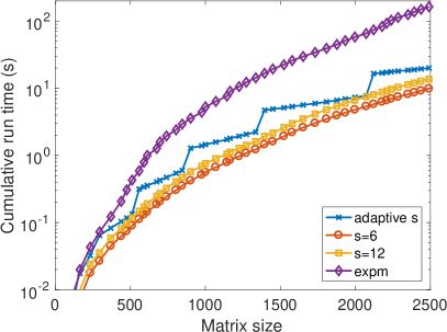
Figure 1: Comparison of incexpm and expm for a random block triangular matrix. Left: Cumulative run time for computing the leading portions. Right: Relative error of incexpm w.r.t. expm.

Figure 1 (left) shows the wall clock time for the incremental computation of all the leading exponentials. Specifically, given $0\leq l\leq n$, each data point shows the time vs. $d_{l}=b_{0}+\cdots+b_{l}$ needed for computing the $l+1$ matrix exponentials $\exp(G_{0}),\exp(G_{1}),\dotsc,\exp(G_{l})$ when using

• expm (by simply applying it to each matrix separately);

• incexpm with the adaptive scaling strategy from Algorithm 6;

• incexpm with fixed scaling power $6$ (scaling used by expm for $G_{0}$);

• incexpm with fixed scaling power $12$ (scaling used by expm for $G_{n}$).

As expected, incexpm is much faster than naively applying expm to each matrix separately; the total times for $l=n$ are also displayed in Table 1. For reference we remark that the run time of Matlab’s expm applied only the final matrix $G_{n}$ is $13.65$s, which is very close to the run time of incexpm with scaling parameter set to $12$ (see Section 2.3 for a discussion of the asymptotic complexity). Indeed, a closer look at the runtime profile of incexpm reveals that the computational overhead induced by the more complicated data structures is largely compensated in the squaring phase by taking advantage of the block triangular matrix structure, from which Matlab’s expm does not profit automatically. It is also interesting to note that the run time of the adaptive scaling strategy is roughly only twice the run time for running the algorithm with a fixed scaling parameter $6$, despite its worse asymptotic complexity.

Table 1: Run time and relative error attained by expm and incexpm on a random block triangular matrix of size $2491$.

Algorithm	Time (s)	Rel. error
expm	163.60
incexpm (adaptive)	20.01	3.27e-15
incexpm ($s=6$)	9.85	2.48e-13
incexpm ($s=12$)	13.70	6.17e-14

The accuracy of the approximations obtained by incexpm is shown on the right in Figure 1. We assume expm as a reference, and measure the relative distance between these two approximations, i.e.,

$$\frac{\lVert\texttt{expm}(G_{l})-\texttt{incexpm}(G_{l})\rVert_{F}}{\lVert\texttt{expm}(G_{l})\rVert_{F}},$$

at each iteration $l$ (quantities smaller than the machine precision are set to $u$ in Figure 1, for plotting purpose). One notes that the approximations of the adaptive strategy remain close to expm throughout the sequence of computations. An observed drop of the error down to $u$ for this strategy corresponds to a restart in Algorithm 6; the approximation at this step is exactly the same as the one of expm. Even for the fixed scaling parameters $6$ and $12$, the obtained approximations are quite accurate.

4.2 Application to option pricing

We now show results for computing option prices using Algorithm 7 for the set of parameters

$$v_{0}=0.04,\quad x_{0}=0,\quad\sigma_{w}=0.5,\quad\mu_{w}=0,\quad\kappa=0.5,\quad\theta=0.04,\quad\sigma=0.15,$$

$$\rho=-0.5,\quad v_{\text{min}}=0.01,\quad v_{\text{max}}=1,\quad r=0,\quad\tau=1/4,\quad k=\log(1.1).$$

We use the tolerance $\epsilon=10^{-3}$ for stopping Algorithm 7.

We explore the use of different algorithms for the computation of the matrix exponentials in line 5 of Algorithm 7: incexpm with adaptive scaling, incexpm with fixed scaling parameter $s=7$ (corresponding to the upper bound from Lemma 3.2 for $n=60$), and expm. Similar to Figure 1, the observed cumulative run times and errors are shown in Figure 2. Again, incexpm is observed to be significantly faster than expm (except for small matrix sizes) while delivering the same level of accuracy. Both incexpm run times are also close to the run time of Matlab’s expm applied only to the final matrix $\tau G_{n}$ ($4.64$s).

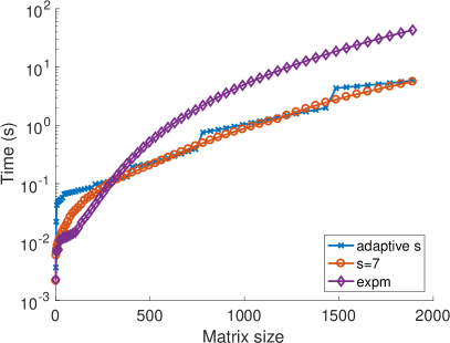
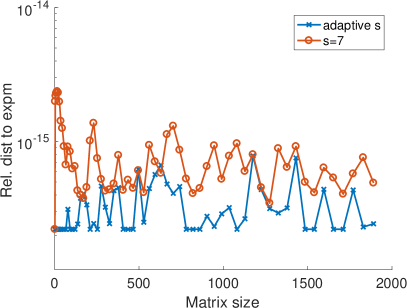
Figure 2: Comparison of incexpm and expm for the block upper triangular matrices arising in the context of the Jacobi model in Algorithm 7. Left: Cumulative run time for computing the leading portions. Right: Relative error of incexpm w.r.t. expm.

Table 2: Total run time and option price errors for the Jacobi model for $n=61$.

Algorithm	Time (s)	Rel. price error
expm	42.97	1.840e-03
incexpm (adaptive)	5.84	1.840e-03
incexpm ($s=7$)	5.60	1.840e-03

Table 2 displays the impact of the different algorithm on the overall Algorithm 7, in terms of execution time and accuracy. Concerning accuracy, we computed the relative error with respect to a reference option price computed by considering a truncation order $n=100$. It can be observed that there is no difference in accuracy for the three algorithms.

Remark 4.1.

The block triangular matrices $G_{n}$ arising from the generator in the Jacobi model actually exhibit additional structure. They are quite sparse and the diagonal blocks are in fact permuted triangular matrices (this does not hold for polynomial diffusion models in general, though). For example, for $n=2$ the matrix $G_{2}$ in the Jacobi model is explicitly given by

$$G_{2}=\left[\begin{array}[]{c|cc|ccc}0&r&\kappa\theta&0&-\frac{\rho\sigma v_{\text{max}}v_{\text{min}}}{S}&-\frac{\sigma^{2}v_{\text{max}}v_{\text{min}}}{S}\\ \hline\cr&0&0&2r&\kappa\theta&0\\ &-\frac{1}{2}&-\kappa&1&r+\frac{\rho\sigma(v_{\text{max}}+v_{\text{min}})}{S}&2\kappa\theta+\frac{\sigma^{2}(v_{\text{max}}+v_{\text{min}})}{S}\\ \hline\cr&&&0&0&0\\ &&&-1&-\kappa&0\\ &&&0&-\frac{1}{2}-\frac{\rho\sigma}{S}&-2\kappa-\frac{\sigma^{2}}{S}\\ \end{array}\right],$$

for $S\mathrel{\mathop{:}}=(\sqrt{v_{\max}}-\sqrt{v_{\min}})^{2}$.

While the particular structure of the diagonal blocks is taken into account automatically by expm and incexpm when computing the LU decompositions of the diagonal blocks, it is not so easy to benefit from the sparsity. Starting from sparse matrix arithmetic, the matrix quickly becomes denser during the evaluation of the initial rational approximation, and in particular during the squaring phase. In all our numerical experiments we used a dense matrix representation throughout.

We repeated the experiments above for the Heston instead of the Jacobi model, that is, we investigated the impact of using our algorithms for computing the matrix exponentials in Algorithm 8. We found that the results for computing the matrix exponentials themselves look very similar to those for the Jacobi model (Figure 2), both in terms of run time and accuracy, so we refrain from giving further details here. There is, however, a notable difference. The evaluation of the stopping criterion requires the solution of two SDPs, which quickly becomes a computational challenge, eventually completely dominating the time needed for the computation of the matrix exponentials.

5 Summary and future work

We have presented techniques for scaling and squaring algorithms that allow for the incremental computation of block triangular matrix exponentials. We combined these techniques with an adaptive scaling strategy that allows for both fast and accurate computation of each matrix exponential in this sequence (Algorithm 6). For our application in polynomial diffusion models, the run time can be further reduced by using fixed scaling parameter, determined through the estimation techniques in Lemmas 3.2 and 3.3.

We observed in our numerical experiments that accurate approximations to these matrix exponentials can be obtained even for quite small, fixed scaling parameters. For the case of two-by-two block triangular matrices, the results of Dieci and Papini [3, 4] support this finding, but an extension of these results to cover a more general setting would be appreciable.

References

- [1] Damien Ackerer, Damir Filipović, and Sergio Pulido. The Jacobi stochastic volatility model. Swiss Finance Institute Research Paper, (16-35), 2016.
- [2] D. A. Bini, S. Dendievel, G. Latouche, and B. Meini. Computing the exponential of large block-triangular block-Toeplitz matrices encountered in fluid queues. Linear Algebra Appl., 502:387–419, 2016.
- [3] Luca Dieci and Alessandra Papini. Padé approximation for the exponential of a block triangular matrix. Linear Algebra Appl., 308(1-3):183–202, 2000.
- [4] Luca Dieci and Alessandra Papini. Conditioning of the exponential of a block triangular matrix. Numer. Algorithms, 28(1-4):137–150, 2001.
- [5] Robert J. Elliott and P. Ekkehard Kopp. Mathematics of Financial Markets. Springer Finance. Springer-Verlag, New York, second edition, 2005.
- [6] Damir Filipović and Martin Larsson. Polynomial diffusions and applications in finance. Finance and Stochastics, pages 1–42, 2016.
- [7] Stefan Güttel and Yuji Nakatsukasa. Scaled and squared subdiagonal Padé approximation for the matrix exponential. SIAM J. Matrix Anal. Appl., 37(1):145–170, 2016.
- [8] Nicholas J. Higham. Functions of Matrices. Society for Industrial and Applied Mathematics (SIAM), Philadelphia, PA, 2008.
- [9] Nicholas J. Higham. The scaling and squaring method for the matrix exponential revisited. SIAM Rev., 51(4):747–764, 2009.
- [10] J. B. Lasserre, T. Prieto-Rumeau, and M. Zervos. Pricing a class of exotic options via moments and SDP relaxations. Math. Finance, 16(3):469–494, 2006.
- [11] Cleve Moler and Charles Van Loan. Nineteen dubious ways to compute the exponential of a matrix, twenty-five years later. SIAM Rev., 45(1):3–49, 2003.
- [12] Bernt Øksendal. Stochastic Differential Equations. Universitext. Springer-Verlag, Berlin, sixth edition, 2003.
- [13] B. N. Parlett. A recurrence among the elements of functions of triangular matrices. Linear Algebra Appl., 14(2):117–121, 1976.