Study on the ${\Upsilon}(1S)$ ${\to}$ $B_{c}D_{s}$ decay

Abstract

The branching ratio and direct $CP$ asymmetry of the ${\Upsilon}(1S)$ ${\to}$ $B_{c}D_{s}$ weak decay are estimated with the perturbative QCD approach firstly. It is found that (1) The direct $CP$-violating asymmetry is close to zero. (2) the branching ratio ${\cal B}r({\Upsilon}(1S){\to}B_{c}D_{s})$ ${\gtrsim}$ $10^{-10}$ might be measurable at the future experiments.

I Introduction

The ${\Upsilon}(1S)$ meson is the ground $S$-wave spin-triplet bottomonium (bound state of $b\bar{b}$) with the well-established quantum number of $I^{G}J^{PC}$ $=$ $0^{-}1^{--}$ pdg . Its mass, $m_{{\Upsilon}(1S)}$ $=$ $9460.30{\pm}0.26$ MeV pdg , is less than the kinematic open-bottom threshold. Phenomenologically, the dominated ${\Upsilon}(1S)$ hadronic decay through the $b\bar{b}$ pairs annihilation into three gluons, with branching ratio ${\cal B}r({\Upsilon}(1S){\to}ggg)$ $=$ $(81.7{\pm}0.7)\%$ pdg , is suppressed by the Okubo-Zweig-Iizuka rule o ; z ; i . The partial width of the ${\Upsilon}(1S)$ electromagnetic decay through the $b\bar{b}$ pairs annihilation into a virtual photon, $(3+R){\Gamma}_{{\ell}^{+}{\ell}^{-}}$, is proportional to $Q_{b}^{2}$, where $Q_{b}$ $=$ $-1/3$ is the electric charge of the bottom quark in the unit of ${|}e{|}$, $R$ is the ratio of the inclusive production cross section of hadrons to the ${\mu}^{+}{\mu}^{-}$ pair production cross section, and ${\Gamma}_{{\ell}^{+}{\ell}^{-}}$ is the partial width of the pure leptonic ${\Upsilon}(1S)$ ${\to}$ ${\ell}^{+}{\ell}^{-}$ decay. Besides, the ${\Upsilon}(1S)$ meson can also decay via the weak interactions within the standard model, although the branching ratio is very small, about $2/{\tau}_{B}{\Gamma}_{{\Upsilon}(1S)}$ ${\sim}$ ${\cal O}(10^{-8})$ pdg , where ${\tau}_{B}$ and ${\Gamma}_{{\Upsilon}(1S)}$ are the lifetime of the $B_{u,d,s}$ meson and the total width of the ${\Upsilon}(1S)$ meson, respectively. In this paper, we will study the ${\Upsilon}(1S)$ ${\to}$ $B_{c}D_{s}$ weak decays with the perturbative QCD (pQCD) approach pqcd1 ; pqcd2 ; pqcd3 . The motivation is listed as follows.

From the experimental point of view, (1) over $10^{8}$ ${\Upsilon}(1S)$ data samples were accumulated by the Belle detector at the KEKB $e^{+}e^{-}$ asymmetric energy collider 1212.5342 . It is hopefully expected that more and more upsilon data samples will be collected with great precision at the forthcoming SuperKEKB and the running upgraded LHC. A large amount of ${\Upsilon}(1S)$ data samples offer a realistic possibility to search for the ${\Upsilon}(1S)$ weak decays which in some cases might be detectable. Theoretical studies on the ${\Upsilon}(1S)$ weak decays are necessary to give a ready reference. (2) For the ${\Upsilon}(1S)$ ${\to}$ $B_{c}D_{s}$ weak decay, the back-to-back final states with opposite electric charges have definite momentums and energies in the center-of-mass frame of the ${\Upsilon}(1S)$ meson. In addition, identification of either a single flavored $D_{s}$ or $B_{c}$ meson is free from the low double-tagging efficiency zpc62.271 , and can provide an unambiguous evidence of the ${\Upsilon}(1S)$ weak decay. Of course, it should be noticed that small branching ratios for the ${\Upsilon}(1S)$ weak decays make the observation extremely challenging, and any evidences of an abnormally large production rate of either a single $D_{s}$ or $B_{c}$ meson might be a hint of new physics zpc62.271 .

From the theoretical point of view, the ${\Upsilon}(1S)$ weak decays permit one to crosscheck parameters obtained from the $b$-flavored hadron decays, to further explore the underlying dynamical mechanism of the heavy quark weak decay, and to test various phenomenological approaches. In recent several years, many attractive methods have been developed to evaluate hadronic matrix elements (HME) where the local quark-level operators are sandwiched between the initial and final hadron states, such as pQCD pqcd1 ; pqcd2 ; pqcd3 , the QCD factorization qcdf2 and the soft and collinear effective theory scet1 ; scet2 ; scet3 ; scet4 , which could give reasonable explanation for many measurements on the nonleptonic $B_{u,d}$ decays. The ${\Upsilon}(1S)$ ${\to}$ $B_{c}D_{s}$ weak decay is favored by the color factor due to the external $W$ emission topological structure, and by the Cabibbo-Kobayashi-Maskawa (CKM) factors ${|}V_{cb}V_{cs}^{\ast}{|}$, so it should have a large branching ratio. However, as far as we know, there is no theoretical investigation on the ${\Upsilon}(1S)$ ${\to}$ $B_{c}D_{s}$ weak decay at the moment. In this paper, we will predict the branching ratio and direct $CP$-violating asymmetry of the ${\Upsilon}(1S)$ ${\to}$ $B_{c}D_{s}$ weak decay with the pQCD approach to confirm whether it is possible to search for this process at the future experiments.

This paper is organized as follows. In section II, we present the theoretical framework and the amplitude for the ${\Upsilon}(1S)$ ${\to}$ $B_{c}D_{s}$ decay. Section III is devoted to numerical results and discussion. Finally, we conclude with a summary in the last section.

II theoretical framework

II.1 The effective Hamiltonian

Using the operator product expansion and renormalization group equation, the effective Hamiltonian responsible for the ${\Upsilon}(1S)$ ${\to}$ $B_{c}D_{s}$ weak decay is written as 9512380

$${\cal H}_{\rm eff}\,=\,\frac{G_{F}}{\sqrt{2}}\,\Big{\{}V_{cb}V_{cs}^{\ast}\sum\limits_{i=1}^{2}C_{i}({\mu})\,Q_{i}({\mu})-V_{tb}V_{ts}^{\ast}\sum\limits_{j=3}^{10}C_{j}({\mu})\,Q_{j}({\mu})\Big{\}}+{\rm H.c.},$$ (1)

where $G_{F}$ $=$ $1.166{\times}10^{-5}\,{\rm GeV}^{-2}$ pdg is the Fermi coupling constant; the CKM factors are expressed as a power series in the Wolfenstein parameter ${\lambda}$ ${\sim}$ $0.2$ pdg ,

$$V_{cb}V_{cs}^{\ast} = +A{\lambda}^{2}-\frac{1}{2}A{\lambda}^{4}-\frac{1}{8}A{\lambda}^{6}(1+4A^{2})+{\cal O}({\lambda}^{8}),$$ (2)

$$V_{tb}V_{ts}^{\ast} = -V_{cb}V_{cs}^{\ast}-A{\lambda}^{4}({\rho}-i{\eta})+{\cal O}({\lambda}^{8}).$$ (3)

The Wilson coefficients $C_{i}(\mu)$ summarize the physical contributions above the scale of ${\mu}$, and have been reliably evaluated to the next-to-leading logarithmic order. The local operators are defined as follows.

$$Q_{1} = [\bar{c}_{\alpha}{\gamma}_{\mu}(1-{\gamma}_{5})b_{\alpha}][\bar{s}_{\beta}{\gamma}^{\mu}(1-{\gamma}_{5})c_{\beta}],$$ (4)

$$Q_{2} = [\bar{c}_{\alpha}{\gamma}_{\mu}(1-{\gamma}_{5})b_{\beta}][\bar{s}_{\beta}{\gamma}^{\mu}(1-{\gamma}_{5})c_{\alpha}],$$ (5)

$$Q_{3} = \sum\limits_{q}[\bar{s}_{\alpha}{\gamma}_{\mu}(1-{\gamma}_{5})b_{\alpha}][\bar{q}_{\beta}{\gamma}^{\mu}(1-{\gamma}_{5})q_{\beta}],$$ (6)

$$Q_{4} = \sum\limits_{q}[\bar{s}_{\alpha}{\gamma}_{\mu}(1-{\gamma}_{5})b_{\beta}][\bar{q}_{\beta}{\gamma}^{\mu}(1-{\gamma}_{5})q_{\alpha}],$$ (7)

$$Q_{5} = \sum\limits_{q}[\bar{s}_{\alpha}{\gamma}_{\mu}(1-{\gamma}_{5})b_{\alpha}][\bar{q}_{\beta}{\gamma}^{\mu}(1+{\gamma}_{5})q_{\beta}],$$ (8)

$$Q_{6} = \sum\limits_{q}[\bar{s}_{\alpha}{\gamma}_{\mu}(1-{\gamma}_{5})b_{\beta}][\bar{q}_{\beta}{\gamma}^{\mu}(1+{\gamma}_{5})q_{\alpha}],$$ (9)

$$Q_{7} = \sum\limits_{q}\frac{3}{2}Q_{q}\,[\bar{s}_{\alpha}{\gamma}_{\mu}(1-{\gamma}_{5})b_{\alpha}][\bar{q}_{\beta}{\gamma}^{\mu}(1+{\gamma}_{5})q_{\beta}],$$ (10)

$$Q_{8} = \sum\limits_{q}\frac{3}{2}Q_{q}\,[\bar{s}_{\alpha}{\gamma}_{\mu}(1-{\gamma}_{5})b_{\beta}][\bar{q}_{\beta}{\gamma}^{\mu}(1+{\gamma}_{5})q_{\alpha}],$$ (11)

$$Q_{9} = \sum\limits_{q}\frac{3}{2}Q_{q}\,[\bar{s}_{\alpha}{\gamma}_{\mu}(1-{\gamma}_{5})b_{\alpha}][\bar{q}_{\beta}{\gamma}^{\mu}(1-{\gamma}_{5})q_{\beta}],$$ (12)

$$Q_{10} = \sum\limits_{q}\frac{3}{2}Q_{q}\,[\bar{s}_{\alpha}{\gamma}_{\mu}(1-{\gamma}_{5})b_{\beta}][\bar{q}_{\beta}{\gamma}^{\mu}(1-{\gamma}_{5})q_{\alpha}],$$ (13)

where $Q_{1,2}$, $Q_{3,{\cdots},6}$, and $Q_{7,{\cdots},10}$ are usually called as the tree operators, QCD penguin operators, and electroweak penguin operators, respectively; ${\alpha}$ and ${\beta}$ are color indices; $q$ denotes all the active quarks at the scale of ${\mu}$ ${\sim}$ ${\cal O}(m_{b})$, i.e., $q$ $=$ $u$, $d$, $s$, $c$, $b$.

II.2 Hadronic matrix elements

To obtain the decay amplitudes, the remaining works are to calculate the hadronic matrix elements of local operators as accurately as possible. Based on the $k_{T}$ factorization theorem npb366 and the Lepage-Brodsky approach for exclusive processes prd22 , HME can be written as the convolution of hard scattering subamplitudes containing perturbative contributions with the universal wave functions reflecting the nonperturbative contributions with the pQCD approach, where the transverse momentums of quarks are retained and the Sudakov factors are introduced, in order to regulate the endpoint singularities and provide a naturally dynamical cutoff on nonperturbative contributions. Usually, the decay amplitude can be factorized into three parts: the hard effects incorporated into the Wilson coefficients $C_{i}$, the process-dependent scattering amplitudes $T$, and the universal wave functions ${\Phi}$, i.e.,

$${\int}dx\,db\,C_{i}(t)\,T(t,x,b)\,{\Phi}(x,b)e^{-S},$$ (14)

where $t$ is a typical scale, $x$ is the longitudinal momentum fraction of the valence quark, $b$ is the conjugate variable of the transverse momentum, and $e^{-S}$ is the Sudakov factor.

II.3 Kinematic variables

The light cone kinematic variables in the ${\Upsilon}(1S)$ rest frame are defined as follows.

$$p_{{\Upsilon}} = p_{1}\,=\,\frac{m_{1}}{\sqrt{2}}(1,1,0),$$ (15)

$$p_{B_{c}} = p_{2}\,=\,(p_{2}^{+},p_{2}^{-},0),$$ (16)

$$p_{D_{s}} = p_{3}\,=\,(p_{3}^{-},p_{3}^{+},0),$$ (17)

$$k_{i} = x_{i}\,p_{i}+(0,0,\vec{k}_{iT}),$$ (18)

$${\epsilon}_{\Upsilon}^{\parallel} = \frac{1}{\sqrt{2}}(1,-1,0),$$ (19)

where $x_{i}$ and $\vec{k}_{iT}$ are the longitudinal momentum fraction and transverse momentum of the valence quark, respectively; ${\epsilon}_{\Upsilon}^{\parallel}$ is the longitudinal polarization vector of the ${\Upsilon}(1S)$ meson. The notation of momentum is showed in Fig.1(a). There are some relations among these kinematic variables.

$$p_{i}^{\pm} = (E_{i}\,{\pm}\,p)/\sqrt{2},$$ (20)

$$s = 2\,p_{2}{\cdot}p_{3},$$ (21)

$$t = 2\,p_{1}{\cdot}p_{2}=2\,m_{1}\,E_{2},$$ (22)

$$u = 2\,p_{1}{\cdot}p_{3}=2\,m_{1}\,E_{3},$$ (23)

$$p=\frac{\sqrt{[m_{1}^{2}-(m_{2}+m_{3})^{2}]\,[m_{1}^{2}-(m_{2}-m_{3})^{2}]}}{2\,m_{1}},$$ (24)

where $p$ is the common momentum of the final $B_{c}$ and $D_{s}$ states; $m_{1}$ $=$ $m_{{\Upsilon}(1S)}$, $m_{2}$ $=$ $m_{B_{c}}$ and $m_{3}$ $=$ $m_{D_{s}}$ denote the masses of the ${\Upsilon}(1S)$, $B_{c}$ and $D_{s}$ mesons, respectively.

II.4 Wave functions

The HME of diquark operators squeezed between the vacuum and ${\Upsilon}(1S)$, $B_{c}$, $D_{s}$ mesons are defined as follows.

$${\langle}0{|}b_{i}(z)\bar{b}_{j}(0){|}{\Upsilon}(p_{1},{\epsilon}_{\parallel}){\rangle}\,=\,\frac{1}{4}f_{\Upsilon}{\int}dk_{1}\,e^{-ik_{1}{\cdot}z}\Big{\{}\!\!\not{\epsilon}_{\parallel}\Big{[}m_{1}\,{\phi}_{\Upsilon}^{v}(k_{1})-\!\!\not{p}_{1}\,{\phi}_{\Upsilon}^{t}(k_{1})\Big{]}\Big{\}}_{ji},$$ (25)

$${\langle}B_{c}^{+}(p_{2}){|}\bar{c}_{i}(z)b_{j}(0){|}0{\rangle}\,=\,\frac{i}{4}f_{B_{c}}{\int}dk_{2}\,e^{ik_{2}{\cdot}z}\,\Big{\{}{\gamma}_{5}\Big{[}\!\!\not{p}_{2}+m_{2}\Big{]}{\phi}_{B_{c}}(k_{2})\Big{\}}_{ji},$$ (26)

$${\langle}D_{s}^{-}(p_{3}){|}\bar{s}_{i}(z)c_{j}(0){|}0{\rangle}\ =\ \frac{i}{4}f_{D_{s}}{\int}_{0}^{1}dk_{3}\,e^{ik_{3}{\cdot}z}\Big{\{}{\gamma}_{5}\Big{[}\!\!\not{p}_{3}+m_{3}\Big{]}{\Phi}_{D_{s}}(k_{3})\Big{\}}_{ji},$$ (27)

where $f_{\Upsilon}$, $f_{B_{c}}$, $f_{D_{s}}$ are decay constants.

There are several phenomenological models for the $D_{s}$ meson wave functions (for example, Eq.(30) in Ref.prd78lv ). In this paper, we will take the model favored by Ref.prd78lv via fitting with measurements on the $B$ ${\to}$ $DP$ decays.

$${\phi}_{D_{s}}(x,b)=6\,x\bar{x}\,\Big{\{}1+C_{D}(1-2\,x)\Big{\}}\,{\exp}\Big{\{}-\frac{1}{2}\,w^{2}\,b^{2}\Big{\}},$$ (28)

where $\bar{x}$ $=$ $1$ $-$ $x$; $x$ and $b$ are the longitudinal momentum fraction and the conjugate variable of the transverse momentum $k_{T}$ of the strange quark in the $D_{s}$ meson, respectively; the exponential term represents the $k_{T}$ distribution; $C_{D}$ $=$ $0.4{\pm}0.1$ and $w$ $=$ $0.2$ GeV prd78lv .

Due to $m_{{\Upsilon}(1S)}$ ${\simeq}$ $2m_{b}$ and $m_{B_{c}}$ ${\simeq}$ $m_{b}$ $+$ $m_{c}$, nonrelativistic quantum chromodynamics prd46 ; prd51 ; rmp77 and Schrödinger equation can be used to describe both ${\Upsilon}(1S)$ and $B_{c}$ mesons. The wave functions of an isotropic harmonic oscillator potential are given in Ref. prd92 ,

$${\phi}_{\Upsilon}^{v}(x)=A\,x\bar{x}\,{\exp}\Big{\{}-\frac{m_{b}^{2}}{8\,{\beta}_{1}^{2}\,x\,\bar{x}}\Big{\}},$$ (29)

$${\phi}_{\Upsilon}^{t}(x)=B\,(x-\bar{x})^{2}\,{\exp}\Big{\{}-\frac{m_{b}^{2}}{8\,{\beta}_{1}^{2}\,x\,\bar{x}}\Big{\}},$$ (30)

$${\phi}_{B_{c}}(x)=C\,x\bar{x}\,{\exp}\Big{\{}-\frac{\bar{x}\,m_{c}^{2}+x\,m_{b}^{2}}{8\,{\beta}_{2}^{2}\,x\,\bar{x}}\Big{\}},$$ (31)

where ${\beta}_{i}$ $=$ ${\xi}_{i}{\alpha}_{s}({\xi}_{i})$ with ${\xi}_{i}$ $=$ $m_{i}/2$; parameters $A$, $B$, $C$ are the normalization coefficients satisfying the following conditions

$${\int}_{0}^{1}dx\,{\phi}_{\Upsilon}^{v,t}(x)=1,\quad{\int}_{0}^{1}dx\,{\phi}_{B_{c}}(x)=1..$$ (32)

II.5 Decay amplitudes

The Feynman diagrams for the ${\Upsilon}(1S)$ ${\to}$ $B_{c}D_{s}$ decay are shown in Fig.1. There are two types: the emission and annihilation topologies, where diagrams containing gluon exchanges between the quarks in the same (different) mesons are entitled (non)factorizable diagrams.

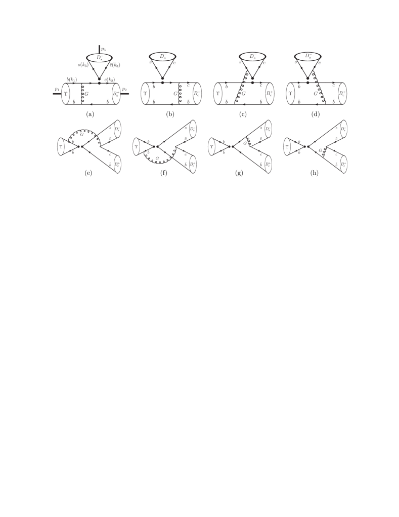
Figure 1: Feynman diagrams for the ${\Upsilon}(1S)$ ${\to}$ $B_{c}D_{s}$ decay with the pQCD approach, including the factorizable emission diagrams (a,b), the nonfactorizable emission diagrams (c,d), the nonfactorizable annihilation diagrams (e,f), and the factorizable annihilation diagrams (g,h).

By calculating these diagrams with the pQCD master formula Eq.(14), the decay amplitudes of ${\Upsilon}(1S)$ ${\to}$ $B_{c}D_{s}$ decay can be expressed as:

$${\cal A}({\Upsilon}(1S){\to}B_{c}D_{s})\ =\ \sqrt{2}\,G_{F}\,{\pi}\,f_{\Upsilon}\,f_{B_{c}}\,f_{D_{s}}\,\frac{C_{F}}{N}\,m_{{\Upsilon}}^{3}\,({\epsilon}_{\Upsilon}{\cdot}p_{D_{s}})$$ (33)

$${\times} \Big{\{}V_{cb}V_{cs}^{\ast}\,\Big{[}{\cal A}_{a+b}^{LL}\,a_{1}+{\cal A}_{c+d}^{LL}\,C_{2}\Big{]}-V_{tb}V_{ts}^{\ast}\,\Big{[}{\cal A}_{a+b}^{LL}\,(a_{4}+a_{10})$$

$$+{\cal A}_{a+b}^{SP}\,(a_{6}+a_{8})+{\cal A}_{c+d}^{LL}\,(C_{3}+C_{9})+{\cal A}_{c+d}^{SP}\,(C_{5}+C_{7})$$

$$+{\cal A}_{e+f}^{LL}\,(C_{3}+C_{4}-\frac{1}{2}C_{9}-\frac{1}{2}C_{10})+{\cal A}_{e+f}^{LR}\,(C_{6}-\frac{1}{2}C_{8})$$

$$+{\cal A}_{g+h}^{LL}\,(a_{3}+a_{4}-\frac{1}{2}a_{9}-\frac{1}{2}a_{10})+{\cal A}_{g+h}^{LR}\,(a_{5}-\frac{1}{2}a_{7})$$

$$+{\cal A}_{e+f}^{SP}\,(C_{5}-\frac{1}{2}C_{7})\Big{]}\Big{\}},$$

where $C_{F}$ $=$ $4/3$ and the color number $N$ $=$ $3$.

The parameters $a_{i}$ are defined as follows.

$$a_{i} = C_{i}+C_{i+1}/N,\quad(i=1,3,5,7,9);$$ (34)

$$a_{i} = C_{i}+C_{i-1}/N,\quad(i=2,4,5,6,10).$$ (35)

The building blocks ${\cal A}_{a+b}$, ${\cal A}_{c+d}$, ${\cal A}_{e+f}$, ${\cal A}_{g+h}$ denote the contributions of the factorizable emission diagrams Fig.1(a,b), the nonfactorizable emission diagrams Fig.1(c,d), the nonfactorizable annihilation diagrams Fig.1(e,f), the factorizable annihilation diagrams Fig.1(g,h), respectively. They are defined as

$${\cal A}_{i+j}^{k}={\cal A}_{i}^{k}+{\cal A}_{j}^{k},$$ (36)

where the subscripts $i$ and $j$ correspond to the indices of Fig.1; the superscript $k$ refers to one of the three possible Dirac structures, namely $k$ $=$ $LL$ for $(V-A){\otimes}(V-A)$, $k$ $=$ $LR$ for $(V-A){\otimes}(V+A)$, and $k$ $=$ $SP$ for $-2(S-P){\otimes}(S+P)$. The explicit expressions of these building blocks are collected in the Appendix A.

III Numerical results and discussion

In the rest frame of the ${\Upsilon}(1S)$ meson, the $CP$-averaged branching ratio and direct $CP$-violating asymmetry for the ${\Upsilon}(1S)$ ${\to}$ $B_{c}D_{s}$ weak decay are written as

$${\cal B}r({\Upsilon}(1S){\to}B_{c}D_{s})\ =\ \frac{1}{12{\pi}}\,\frac{p}{m_{{\Upsilon}}^{2}{\Gamma}_{{\Upsilon}}}\,{|}{\cal A}({\Upsilon}(1S){\to}B_{c}D_{s}){|}^{2},$$ (37)

$${\cal A}_{\rm CP}({\Upsilon}(1S){\to}B_{c}D_{s})\ =\ \frac{{\cal B}r({\Upsilon}(1S){\to}B_{c}^{+}D_{s}^{-})-{\cal B}r({\Upsilon}(1S){\to}B_{c}^{-}D_{s}^{+})}{{\cal B}r({\Upsilon}(1S){\to}B_{c}^{+}D_{s}^{-})+{\cal B}r({\Upsilon}(1S){\to}B_{c}^{-}D_{s}^{+})},$$ (38)

where the decay width ${\Gamma}_{\Upsilon}$ $=$ $54.02{\pm}1.25$ keV pdg .

The numerical values of other input parameters are listed as follows.

(1) The Wolfenstein parameters pdg : $A$ $=$ $0.814^{+0.023}_{-0.024}$, ${\lambda}$ $=$ $0.22537{\pm}0.00061$, $\bar{\rho}$ $=$ $0.117{\pm}0.021$, and $\bar{\eta}$ $=$ $0.353{\pm}0.013$, where $({\rho}+i{\eta})$ $=$ $(\bar{\rho}+i\bar{\eta})(1+{\lambda}^{2}/2+{\cdots})$.

(2) Masses of quarks pdg : $m_{c}$ $=$ $1.67{\pm}0.07$ GeV and $m_{b}$ $=$ $4.78{\pm}0.06$ GeV.

(3) Decay constants: $f_{{\Upsilon}(1S)}$ $=$ $676.4{\pm}10.7$ MeV prd92 , $f_{B_{c}}$ $=$ $489{\pm}5$ MeV fbc , and $f_{D_{s}}$ $=$ $257.5{\pm}4.6$ MeV pdg .

Finally, we get

$${\cal B}r({\Upsilon}(1S){\to}B_{c}D_{s})\ =\ (3.78^{+0.27+0.42+0.50+0.34}_{-0.26-0.38-0.25-0.32}){\times}10^{-10},$$ (39)

$${\cal A}_{\rm CP}({\Upsilon}(1S){\to}B_{c}D_{s})\ =\ (4.79^{+0.21+1.14+0.18+0.36}_{-0.20-1.00-0.44-0.39}){\times}10^{-5},$$ (40)

where the central values are obtained with the central values of input parameters; the first uncertainties come from the CKM parameters; the second uncertainties are due to the variation of mass $m_{b}$ and $m_{c}$; the third uncertainties arise from the typical scale ${\mu}$ $=$ $(1{\pm}0.1)t_{i}$, where the expressions of $t_{i}$ for different topologies are given in Eqs.(71-74); and the fourth uncertainties correspond to the variation of decay constants $f_{\Upsilon}$, $f_{B_{c}}$, $f_{D_{s}}$ and shape parameter $C_{D}$ in Eq.(28). There are some comments.

(1) It is seen from Eq.(39) that branching ratio for the ${\Upsilon}(1S)$ ${\to}$ $B_{c}D_{s}$ decay can reach up to $10^{-10}$, which might be accessible at the running LHC and forthcoming SuperKEKB. For example, the ${\Upsilon}(1S)$ production cross section in p-Pb collision is a few ${\mu}b$ with the LHCb jhep1407 and ALICE plb740 detectors at LHC. Over $10^{12}$ ${\Upsilon}(1S)$ mesons per $ab^{-1}$ data collected at LHCb and ALICE are in principle available, corresponding to a few hundreds of the ${\Upsilon}(1S)$ ${\to}$ $B_{c}D_{s}$ events.

(2) Compared the ${\Upsilon}(1S)$ ${\to}$ $B_{c}D_{s}$ decay with the ${\Upsilon}(1S)$ ${\to}$ $B_{c}{\pi}$ decay prd92 , they are both the color-favored and CKM-favored. There is only the emission topologies and only the tree operators contributing to the ${\Upsilon}(1S)$ ${\to}$ $B_{c}{\pi}$ decay. Besides the emission topologies and tree operators, there are other contributions from the annihilation topologies and penguin operators for the ${\Upsilon}(1S)$ ${\to}$ $B_{c}D_{s}$ decay. In addition, there is another important factor, the decay constant $f_{D_{s}}$ $>$ $2f_{\pi}$. This might explain the fact that although the final phase spaces for the ${\Upsilon}(1S)$ ${\to}$ $B_{c}D_{s}$ decay is more compact than those for the ${\Upsilon}(1S)$ ${\to}$ $B_{c}{\pi}$ decay, there is still the relation, ${\cal B}r({\Upsilon}(1S){\to}B_{c}D_{s})$ $>$ ${\cal B}r({\Upsilon}(1S){\to}B_{c}{\pi})$ with the pQCD approach.

(3) It is shown from Eq.(40) that the direct $CP$ asymmetry for the ${\Upsilon}(1S)$ ${\to}$ $B_{c}D_{s}$ decay is close to zero. The fact should be so. As it is well known, the magnitude of direct $CP$ asymmetry is proportional to the sine of weak phase difference. First and foremost, the weak phase difference between the CKM factors $V_{cb}V_{cs}^{\ast}$ and $V_{tb}V_{ts}^{\ast}$ are suppressed by the factor of ${\lambda}^{2}$. Secondly, compared with the tree contributions appearing with $V_{cb}V_{cs}^{\ast}$, the penguin and annihilation contributions always accompanied with $V_{tb}V_{ts}^{\ast}$ are suppressed by the small Wilson coefficients.

(4) As it is well known, due to mass $m_{B_{c}}$ $>$ $m_{{\Upsilon}(1S)}/2$, the momentum transition in the ${\Upsilon}(1S)$ ${\to}$ $B_{c}D_{s}$ decay may be not large enough. One might question whether the pQCD approach is applicable and whether the perturbative calculation is reliable. Therefore, it is necessary to check what percentage of the contributions comes from the perturbative region. The contributions to branching ratio from different region of ${\alpha}_{s}/{\pi}$ are showed in Fig.(2). One can clearly see from Fig.(2) that more than 90% contributions to branching ratio come from the ${\alpha}_{s}/{\pi}$ ${\leq}$ $0.3$ region, and the contributions from nonperturbative region with large ${\alpha}_{s}/{\pi}$ are highly suppressed. One important reason is that assisting with the typical scale in Eqs.(71-74), the quark transverse momentum is retained and the Sudakov factor is introduced to effectively suppress the nonperturbative contributions within the pQCD approach pqcd1 ; pqcd2 ; pqcd3 .

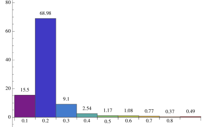
Figure 2: The contributions to the branching ratio from different region of ${\alpha}_{s}/{\pi}$ (horizontal axises), where the numbers over histogram denote the percentage of the corresponding contributions.

(5) There are many uncertainties on our results. Other factors, such as the contributions of higher order corrections to HME, relativistic effects and so on, which are not considered here, deserve the dedicated study. Our results just provide an order of magnitude estimation.

IV Summary

The ${\Upsilon}(1S)$ weak decay is legal within the standard model. With the potential prospects of the ${\Upsilon}(1S)$ at high-luminosity dedicated heavy-flavor factories, the ${\Upsilon}(1S)$ ${\to}$ $B_{c}D_{s}$, weak decays are studied with the pQCD approach. It is found that with the nonrelativistic wave functions for ${\Upsilon}(1S)$ and $B_{c}$ mesons, branching ratios ${\cal B}r({\Upsilon}(1S){\to}B_{c}D_{s})$ ${\gtrsim}$ $10^{-10}$, which might be measurable in future experiments. The direct $CP$-violating asymmetry for the ${\Upsilon}(1S)$ ${\to}$ $B_{c}D_{s}$ decay is close to zero because of the tiny weak phase difference.

Appendix A The building blocks of decay amplitudes

For the sake of simplicity, we decompose the decay amplitude Eq.(33) into some building blocks ${\cal A}_{i}^{k}$, where the subscript $i$ on ${\cal A}_{i}^{k}$ corresponds to the indices of Fig.1; the superscript $k$ on ${\cal A}_{i}^{k}$ refers to one of the three possible Dirac structures ${\Gamma}_{1}{\otimes}{\Gamma}_{2}$ of the four-quark operator $(\bar{q}_{1}{\Gamma}_{1}q_{2})(\bar{q}_{1}{\Gamma}_{2}q_{2})$, namely $k$ $=$ $LL$ for $(V-A){\otimes}(V-A)$, $k$ $=$ $LR$ for $(V-A){\otimes}(V+A)$, and $k$ $=$ $SP$ for $-2(S-P){\otimes}(S+P)$. The explicit expressions of ${\cal A}_{i}^{k}$ are written as follows.

$${\cal A}_{a}^{LL} = {\int}_{0}^{1}dx_{1}{\int}_{0}^{1}dx_{2}{\int}_{0}^{\infty}b_{1}db_{1}{\int}_{0}^{\infty}b_{2}db_{2}\,{\phi}_{\Upsilon}^{v}(x_{1})\,{\phi}_{B_{c}}(x_{2})$$ (41)

$$E_{a}(t_{a})\,{\alpha}_{s}(t_{a})\,H_{ab}({\alpha}_{e},{\beta}_{a},b_{1},b_{2})\,\Big{\{}x_{2}+r_{3}^{2}\bar{x}_{2}+r_{2}r_{b}\Big{\}},$$

$${\cal A}_{a}^{SP} = -2\,r_{3}\,{\int}_{0}^{1}dx_{1}{\int}_{0}^{1}dx_{2}{\int}_{0}^{\infty}b_{1}db_{1}{\int}_{0}^{\infty}b_{2}db_{2}\,{\phi}_{\Upsilon}^{v}(x_{1})\,{\phi}_{B_{c}}(x_{2})$$ (42)

$$E_{a}(t_{a})\,{\alpha}_{s}(t_{a})\,H_{ab}({\alpha}_{e},{\beta}_{a},b_{1},b_{2})\,\Big{\{}r_{b}+r_{2}\bar{x}_{2}\Big{\}},$$

$${\cal A}_{b}^{LL} = {\int}_{0}^{1}dx_{1}{\int}_{0}^{1}dx_{2}{\int}_{0}^{\infty}b_{1}db_{1}{\int}_{0}^{\infty}b_{2}db_{2}\,{\phi}_{B_{c}}(x_{2})\,E_{b}(t_{b})\,{\alpha}_{s}(t_{b})$$ (43)

$$H_{ab}({\alpha}_{e},{\beta}_{b},b_{2},b_{1})\,\Big{\{}{\phi}_{\Upsilon}^{v}(x_{1})\Big{[}2\,r_{2}\,r_{c}-r_{2}^{2}\,x_{1}-r_{3}^{2}\,\bar{x}_{1}\Big{]}$$

$$+{\phi}_{\Upsilon}^{t}(x_{1})\Big{[}2\,r_{2}\,x_{1}-r_{c}\Big{]}\Big{\}},$$

$${\cal A}_{b}^{SP} = -2\,r_{3}\,{\int}_{0}^{1}dx_{1}{\int}_{0}^{1}dx_{2}{\int}_{0}^{\infty}b_{1}db_{1}{\int}_{0}^{\infty}b_{2}db_{2}\,{\phi}_{B_{c}}(x_{2})\,E_{b}(t_{b})\,{\alpha}_{s}(t_{b})$$ (44)

$$H_{ab}({\alpha}_{e},{\beta}_{b},b_{2},b_{1})\,\Big{\{}{\phi}_{\Upsilon}^{v}(x_{1})\,(2\,r_{2}-r_{c})-{\phi}_{\Upsilon}^{t}(x_{1})\,\bar{x}_{1}\Big{\}},$$

$${\cal A}_{c}^{LL} = \frac{1}{N}{\int}_{0}^{1}dx_{1}{\int}_{0}^{1}dx_{2}{\int}_{0}^{1}dx_{3}{\int}_{0}^{\infty}db_{1}{\int}_{0}^{\infty}b_{2}db_{2}{\int}_{0}^{\infty}b_{3}db_{3}\,{\delta}(b_{1}-b_{2})$$ (45)

$${\phi}_{B_{c}}(x_{2})\,{\phi}_{D_{s}}(x_{3},b_{3})\,E_{c}(t_{c})\,{\alpha}_{s}(t_{c})\,H_{cd}({\alpha}_{e},{\beta}_{c},b_{2},b_{3})\,\Big{\{}{\phi}_{\Upsilon}^{v}(x_{1})$$

$$\Big{[}\frac{s\,(x_{1}-\bar{x}_{3})}{m_{1}^{2}}\,+2\,r_{2}^{2}\,(x_{1}-x_{2})\Big{]}+{\phi}_{\Upsilon}^{t}(x_{1})\,r_{2}\,(x_{2}-x_{1})\Big{\}},$$

$${\cal A}_{c}^{SP} = -\frac{1}{N}\,r_{3}{\int}_{0}^{1}dx_{1}{\int}_{0}^{1}dx_{2}{\int}_{0}^{1}dx_{3}{\int}_{0}^{\infty}db_{1}{\int}_{0}^{\infty}b_{2}db_{2}{\int}_{0}^{\infty}b_{3}db_{3}\,{\alpha}_{s}(t_{c})$$ (46)

$${\delta}(b_{1}-b_{2})\,{\phi}_{B_{c}}(x_{2})\,{\phi}_{D_{s}}(x_{3},b_{3})\,E_{c}(t_{c})\,H_{cd}({\alpha}_{e},{\beta}_{c},b_{2},b_{3})$$

$$\Big{\{}{\phi}_{\Upsilon}^{v}(x_{1})\,r_{2}\,(\bar{x}_{3}-x_{2})+{\phi}_{\Upsilon}^{t}(x_{1})\,(x_{1}-\bar{x}_{3})\Big{\}},$$

$${\cal A}_{d}^{LL} = \frac{1}{N}{\int}_{0}^{1}dx_{1}{\int}_{0}^{1}dx_{2}{\int}_{0}^{1}dx_{3}{\int}_{0}^{\infty}db_{1}{\int}_{0}^{\infty}b_{2}db_{2}{\int}_{0}^{\infty}b_{3}db_{3}\,{\delta}(b_{1}-b_{2})$$ (47)

$${\phi}_{B_{c}}(x_{2})\,{\phi}_{D_{s}}(x_{3},b_{3})\,E_{d}(t_{d})\,{\alpha}_{s}(t_{d})\,H_{cd}({\alpha}_{e},{\beta}_{d},b_{2},b_{3})\,\Big{\{}{\phi}_{\Upsilon}^{v}(x_{1})$$

$$\Big{[}\frac{s\,(x_{3}-x_{2})}{m_{1}^{2}}-r_{3}\,r_{c}\Big{]}+{\phi}_{\Upsilon}^{t}(x_{1})\,r_{2}\,(x_{2}-x_{1})\Big{\}},$$

$${\cal A}_{d}^{SP} = -\frac{1}{N}\,r_{3}{\int}_{0}^{1}dx_{1}{\int}_{0}^{1}dx_{2}{\int}_{0}^{1}dx_{3}{\int}_{0}^{\infty}db_{1}{\int}_{0}^{\infty}b_{2}db_{2}{\int}_{0}^{\infty}b_{3}db_{3}\,{\alpha}_{s}(t_{d})$$ (48)

$${\delta}(b_{1}-b_{2})\,{\phi}_{B_{c}}(x_{2})\,{\phi}_{D_{s}}(x_{3},b_{3})\,E_{d}(t_{d})\,H_{cd}({\alpha}_{e},{\beta}_{d},b_{2},b_{3})$$

$$\Big{\{}{\phi}_{\Upsilon}^{v}(x_{1})\,r_{2}\,(r_{c}/r_{3}+x_{2}-x_{3})+{\phi}_{\Upsilon}^{t}(x_{1})\,(x_{3}-x_{1}-r_{c}/r_{3})\Big{\}},$$

$${\cal A}_{e}^{LL} = \frac{1}{N}{\int}_{0}^{1}dx_{1}{\int}_{0}^{1}dx_{2}{\int}_{0}^{1}dx_{3}{\int}_{0}^{\infty}b_{1}db_{1}{\int}_{0}^{\infty}b_{2}db_{2}{\int}_{0}^{\infty}db_{3}\,{\delta}(b_{2}-b_{3})$$ (49)

$${\phi}_{B_{c}}(x_{2})\,{\phi}_{D_{s}}(x_{3},b_{3})\,E_{e}(t_{e})\,{\alpha}_{s}(t_{e})\,H_{ef}({\alpha}_{a},{\beta}_{e},b_{1},b_{2})\,\Big{\{}{\phi}_{\Upsilon}^{v}(x_{1})$$

$$\Big{[}\frac{s\,(x_{1}-\bar{x}_{3})}{m_{1}^{2}}+2\,r_{2}^{2}\,(x_{1}-x_{2})+r_{2}\,r_{3}\,(x_{2}-\bar{x}_{3})\Big{]}-r_{b}\,{\phi}_{\Upsilon}^{t}(x_{1})\Big{\}},$$

$${\cal A}_{e}^{LR} = \frac{1}{N}{\int}_{0}^{1}dx_{1}{\int}_{0}^{1}dx_{2}{\int}_{0}^{1}dx_{3}{\int}_{0}^{\infty}b_{1}db_{1}{\int}_{0}^{\infty}b_{2}db_{2}{\int}_{0}^{\infty}db_{3}\,{\delta}(b_{2}-b_{3})$$ (50)

$${\phi}_{B_{c}}(x_{2})\,{\phi}_{D_{s}}(x_{3},b_{3})\,E_{e}(t_{e})\,{\alpha}_{s}(t_{e})\,H_{ef}({\alpha}_{a},{\beta}_{e},b_{1},b_{2})\,\Big{\{}{\phi}_{\Upsilon}^{v}(x_{1})$$

$$\Big{[}\frac{s\,(x_{2}-x_{1})}{m_{1}^{2}}+2\,r_{3}^{2}\,(\bar{x}_{3}-x_{1})+r_{2}\,r_{3}\,(x_{2}-\bar{x}_{3})\Big{]}+r_{b}\,{\phi}_{\Upsilon}^{t}(x_{1})\Big{\}},$$

$${\cal A}_{e}^{SP} = \frac{1}{N}{\int}_{0}^{1}dx_{1}{\int}_{0}^{1}dx_{2}{\int}_{0}^{1}dx_{3}{\int}_{0}^{\infty}b_{1}db_{1}{\int}_{0}^{\infty}b_{2}db_{2}{\int}_{0}^{\infty}db_{3}\,{\delta}(b_{2}-b_{3})$$ (51)

$${\phi}_{B_{c}}(x_{2})\,{\phi}_{D_{s}}(x_{3},b_{3})\,E_{e}(t_{e})\,{\alpha}_{s}(t_{e})\,H_{ef}({\alpha}_{a},{\beta}_{e},b_{1},b_{2})$$

$$\Big{\{}{\phi}_{\Upsilon}^{v}(x_{1})\,r_{b}\,(r_{2}+r_{3})+{\phi}_{\Upsilon}^{t}(x_{1})\Big{[}r_{2}\,(x_{2}-x_{1})+r_{3}\,(\bar{x}_{3}-x_{1})\Big{]}\Big{\}},$$

$${\cal A}_{f}^{LL} = \frac{1}{N}{\int}_{0}^{1}dx_{1}{\int}_{0}^{1}dx_{2}{\int}_{0}^{1}dx_{3}{\int}_{0}^{\infty}b_{1}db_{1}{\int}_{0}^{\infty}b_{2}db_{2}{\int}_{0}^{\infty}db_{3}\,{\delta}(b_{2}-b_{3})$$ (52)

$${\phi}_{B_{c}}(x_{2})\,{\phi}_{D_{s}}(x_{3},b_{3})\,E_{f}(t_{f})\,{\alpha}_{s}(t_{f})\,H_{ef}({\alpha}_{a},{\beta}_{e},b_{1},b_{2})\,\Big{\{}{\phi}_{\Upsilon}^{v}(x_{1})$$

$$\Big{[}\frac{s\,(\bar{x}_{1}-x_{2})}{m_{1}^{2}}+2\,r_{3}^{2}\,(x_{3}-x_{1})+r_{2}\,r_{3}\,(\bar{x}_{3}-x_{2})\Big{]}-r_{b}\,{\phi}_{\Upsilon}^{t}(x_{1})\Big{\}},$$

$${\cal A}_{f}^{LR} = \frac{1}{N}{\int}_{0}^{1}dx_{1}{\int}_{0}^{1}dx_{2}{\int}_{0}^{1}dx_{3}{\int}_{0}^{\infty}b_{1}db_{1}{\int}_{0}^{\infty}b_{2}db_{2}{\int}_{0}^{\infty}db_{3}\,{\delta}(b_{2}-b_{3})$$ (53)

$${\phi}_{B_{c}}(x_{2})\,{\phi}_{D_{s}}(x_{3},b_{3})\,E_{f}(t_{f})\,{\alpha}_{s}(t_{f})\,H_{ef}({\alpha}_{a},{\beta}_{e},b_{1},b_{2})\,\Big{\{}{\phi}_{\Upsilon}^{v}(x_{1})$$

$$\Big{[}\frac{s\,(x_{1}-x_{3})}{m_{1}^{2}}+2\,r_{2}^{2}\,(x_{2}-\bar{x}_{1})+r_{2}\,r_{3}\,(\bar{x}_{3}-x_{2})\Big{]}+r_{b}\,{\phi}_{\Upsilon}^{t}(x_{1})\Big{\}},$$

$${\cal A}_{f}^{SP} = \frac{1}{N}{\int}_{0}^{1}dx_{1}{\int}_{0}^{1}dx_{2}{\int}_{0}^{1}dx_{3}{\int}_{0}^{\infty}b_{1}db_{1}{\int}_{0}^{\infty}b_{2}db_{2}{\int}_{0}^{\infty}db_{3}\,{\delta}(b_{2}-b_{3})$$ (54)

$${\phi}_{B_{c}}(x_{2})\,{\phi}_{D_{s}}(x_{3},b_{3})\,E_{f}(t_{f})\,{\alpha}_{s}(t_{f})\,H_{ef}({\alpha}_{a},{\beta}_{e},b_{1},b_{2})$$

$$\Big{\{}{\phi}_{\Upsilon}^{v}(x_{1})\,r_{b}\,(r_{2}+r_{3})+{\phi}_{\Upsilon}^{t}(x_{1})\Big{[}r_{2}\,(x_{2}-\bar{x}_{1})+r_{3}\,(x_{1}-x_{3})\Big{]}\Big{\}},$$

$${\cal A}_{g}^{LL} = {\cal A}_{g}^{LR}={\int}_{0}^{1}dx_{2}{\int}_{0}^{1}dx_{3}{\int}_{0}^{\infty}b_{2}db_{2}{\int}_{0}^{\infty}b_{3}db_{3}\,{\phi}_{B_{c}}(x_{2})\,{\phi}_{D_{s}}(x_{3},b_{3})$$ (55)

$$E_{f}(t_{g})\,{\alpha}_{s}(t_{g})\,H_{gh}({\alpha}_{a},{\beta}_{g},b_{2},b_{3})\,\Big{\{}x_{2}+r_{3}\,\bar{x}_{2}\,(r_{3}-2\,r_{2})\Big{\}},$$

$${\cal A}_{h}^{LL} = {\cal A}_{h}^{LR}={\int}_{0}^{1}dx_{2}{\int}_{0}^{1}dx_{3}{\int}_{0}^{\infty}b_{2}db_{2}{\int}_{0}^{\infty}b_{3}db_{3}\,{\phi}_{B_{c}}(x_{2})\,{\phi}_{D_{s}}(x_{3},b_{3})$$ (56)

$$E_{h}(t_{h})\,{\alpha}_{s}(t_{h})\,H_{gh}({\alpha}_{a},{\beta}_{h},b_{3},b_{2})\,\Big{\{}\bar{x}_{3}+r_{2}\,x_{3}\,(r_{2}-2\,r_{3})$$

$$+r_{b}\,(r_{3}-2\,r_{2})\Big{\}},$$

where the mass ratio $r_{i}$ $=$ $m_{i}/m_{1}$; $\bar{x}_{i}$ $=$ $1$ $-$ $x_{i}$; variable $x_{i}$ is the longitudinal momentum fraction of the valence quark; $b_{i}$ is the conjugate variable of the transverse momentum $k_{i{\perp}}$; and ${\alpha}_{s}(t)$ is the QCD coupling at the scale of $t$.

The function $H_{i}$ are defined as follows.

$$H_{ab}({\alpha}_{e},{\beta},b_{i},b_{j}) = K_{0}(\sqrt{-{\alpha}_{e}}b_{i})\Big{\{}{\theta}(b_{i}-b_{j})K_{0}(\sqrt{-{\beta}}b_{i})I_{0}(\sqrt{-{\beta}}b_{j})+(b_{i}{\leftrightarrow}b_{j})\Big{\}},$$ (57)

$$H_{cd}({\alpha}_{e},{\beta},b_{2},b_{3}) = \Big{\{}{\theta}(-{\beta})K_{0}(\sqrt{-{\beta}}b_{3})+\frac{{\pi}}{2}{\theta}({\beta})\Big{[}iJ_{0}(\sqrt{{\beta}}b_{3})-Y_{0}(\sqrt{{\beta}}b_{3})\Big{]}\Big{\}}$$ (58)

$${\times} \Big{\{}{\theta}(b_{2}-b_{3})K_{0}(\sqrt{-{\alpha}_{e}}b_{2})I_{0}(\sqrt{-{\alpha}_{e}}b_{3})+(b_{2}{\leftrightarrow}b_{3})\Big{\}},$$

$$H_{ef}({\alpha}_{a},{\beta},b_{1},b_{2}) = \Big{\{}{\theta}(-{\beta})K_{0}(\sqrt{-{\beta}}b_{1})+\frac{{\pi}}{2}{\theta}({\beta})\Big{[}iJ_{0}(\sqrt{{\beta}}b_{1})-Y_{0}(\sqrt{{\beta}}b_{1})\Big{]}\Big{\}}$$ (59)

$$\!\!\!\!\!\!\!\!\!\!\!\!\!\!\!\!\!\!\!\!\!\!\!\!{\times}\frac{{\pi}}{2}\Big{\{}{\theta}(b_{1}-b_{2})\Big{[}iJ_{0}(\sqrt{{\alpha}_{a}}b_{1})-Y_{0}(\sqrt{{\alpha}_{a}}b_{1})\Big{]}J_{0}(\sqrt{{\alpha}_{a}}b_{2})+(b_{1}{\leftrightarrow}b_{2})\Big{\}},$$

$$H_{hg}({\alpha}_{a},{\beta},b_{i},b_{j}) = \frac{{\pi}^{2}}{4}\Big{\{}iJ_{0}(\sqrt{{\alpha}_{a}}b_{j})-Y_{0}(\sqrt{{\alpha}_{a}}b_{j})\Big{\}}$$ (60)

$${\times} \Big{\{}{\theta}(b_{i}-b_{j})\Big{[}iJ_{0}(\sqrt{{\beta}}b_{i})-Y_{0}(\sqrt{{\beta}}b_{i})\Big{]}J_{0}(\sqrt{{\beta}}b_{j})+(b_{i}{\leftrightarrow}b_{j})\Big{\}},$$

where $J_{0}$ and $Y_{0}$ ($I_{0}$ and $K_{0}$) are the (modified) Bessel function of the first and second kind, respectively; ${\alpha}_{e}$ (${\alpha}_{a}$) is the gluon virtuality of the emission (annihilation) diagrams; the subscript of the quark virtuality ${\beta}_{i}$ corresponds to the indices of Fig.1. The definition of the particle virtuality is listed as follows.

$${\alpha}_{e} = \bar{x}_{1}^{2}m_{1}^{2}+\bar{x}_{2}^{2}m_{2}^{2}-\bar{x}_{1}\bar{x}_{2}t,$$ (61)

$${\alpha}_{a} = x_{2}^{2}m_{2}^{2}+\bar{x}_{3}^{2}m_{3}^{2}+x_{2}\bar{x}_{3}s,$$ (62)

$${\beta}_{a} = m_{1}^{2}-m_{b}^{2}+\bar{x}_{2}^{2}m_{2}^{2}-\bar{x}_{2}t,$$ (63)

$${\beta}_{b} = m_{2}^{2}-m_{c}^{2}+\bar{x}_{1}^{2}m_{1}^{2}-\bar{x}_{1}t,$$ (64)

$${\beta}_{c} = x_{1}^{2}m_{1}^{2}+x_{2}^{2}m_{2}^{2}+\bar{x}_{3}^{2}m_{3}^{2}$$ (65)

$$- x_{1}x_{2}t-x_{1}\bar{x}_{3}u+x_{2}\bar{x}_{3}s,$$

$${\beta}_{d} = x_{1}^{2}m_{1}^{2}+x_{2}^{2}m_{2}^{2}+x_{3}^{2}m_{3}^{2}-m_{c}^{2}$$ (66)

$$- x_{1}x_{2}t-x_{1}x_{3}u+x_{2}x_{3}s,$$

$${\beta}_{e} = x_{1}^{2}m_{1}^{2}+x_{2}^{2}m_{2}^{2}+\bar{x}_{3}^{2}m_{3}^{2}-m_{b}^{2}$$ (67)

$$- x_{1}x_{2}t-x_{1}\bar{x}_{3}u+x_{2}\bar{x}_{3}s,$$

$${\beta}_{f} = \bar{x}_{1}^{2}m_{1}^{2}+x_{2}^{2}m_{2}^{2}+\bar{x}_{3}^{2}m_{3}^{2}-m_{b}^{2}$$ (68)

$$- \bar{x}_{1}x_{2}t-\bar{x}_{1}\bar{x}_{3}u+x_{2}\bar{x}_{3}s,$$

$${\beta}_{g} = x_{2}^{2}m_{2}^{2}+m_{3}^{2}+x_{2}s,$$ (69)

$${\beta}_{h} = \bar{x}_{3}^{2}m_{3}^{2}+m_{2}^{2}+\bar{x}_{3}s-m_{b}^{2}.$$ (70)

The typical scale $t_{i}$ and the Sudakov factor $E_{i}$ are defined as follows, where the subscript $i$ corresponds to the indices of Fig.1.

$$t_{a(b)} = {\max}(\sqrt{-{\alpha}_{e}},\sqrt{-{\beta}_{a(b)}},1/b_{1},1/b_{2}),$$ (71)

$$t_{c(d)} = {\max}(\sqrt{-{\alpha}_{e}},\sqrt{{|}{\beta}_{c(d)}{|}},1/b_{2},1/b_{3}),$$ (72)

$$t_{e(f)} = {\max}(\sqrt{{\alpha}_{a}},\sqrt{{|}{\beta}_{e(f)}{|}},1/b_{1},1/b_{2}),$$ (73)

$$t_{g(h)} = {\max}(\sqrt{{\alpha}_{a}},\sqrt{{\beta}_{g(h)}},1/b_{2},1/b_{3}),$$ (74)

$$E_{i}(t)=\left\{\begin{array}[]{lll}{\exp}\{-S_{{\Upsilon}(1S)}(t)-S_{B_{c}}(t)\},&{}&i=a,b\\ {\exp}\{-S_{{\Upsilon}(1S)}(t)-S_{B_{c}}(t)-S_{D_{s}}(t)\},&&i=c,d,e,f\\ {\exp}\{-S_{B_{c}}(t)-S_{D_{s}}(t)\},&&i=g,h\end{array}\right.$$ (75)

$$S_{{\Upsilon}(1S)}(t) = s(x_{1},p_{1}^{+},1/b_{1})+2{\int}_{1/b_{1}}^{t}\frac{d{\mu}}{\mu}{\gamma}_{q},$$ (76)

$$S_{B_{c}}(t) = s(x_{2},p_{2}^{+},1/b_{2})+2{\int}_{1/b_{2}}^{t}\frac{d{\mu}}{\mu}{\gamma}_{q},$$ (77)

$$S_{D_{s}}(t) = s(x_{3},p_{3}^{+},1/b_{3})+2{\int}_{1/b_{3}}^{t}\frac{d{\mu}}{\mu}{\gamma}_{q},$$ (78)

where ${\gamma}_{q}$ $=$ $-{\alpha}_{s}/{\pi}$ is the quark anomalous dimension; the explicit expression of $s(x,Q,1/b)$ can be found in the appendix of Ref.pqcd1 .

References

- (1) K. Olive et al. (Particle Data Group), Chin. Phys. C 38, 090001 (2014).
- (2) S. Okubo, Phys. Lett. 5, 165 (1963).
- (3) G. Zweig, CERN-TH-401, 402, 412 (1964).
- (4) J. Iizuka, Prog. Theor. Phys. Suppl. 37-38, 21 (1966).
- (5) C. Patrignani, T. Pedlar, and J. Rosner, Annu. Rev. Nucl. Part. Sci. 63, 21 (2013).
- (6) H. Li, Phys. Rev. D 52, 3958 (1995).
- (7) C. Chang, H. Li, Phys. Rev. D 55, 5577 (1997).
- (8) T. Yeh, H. Li, Phys. Rev. D 56, 1615 (1997).
- (9) J. Brodzicka et al. (Belle Collaboration), Prog. Theor. Exp. Phys. 2012, 04D001.
- (10) M. Sanchis-Lozano, Z. Phys. C 62, 271 (1994).
- (11) M. Beneke et al., Nucl. Phys. B 591, 313 (2000).
- (12) C. Bauer et al., Phys. Rev. D 63, 114020 (2001).
- (13) C. Bauer, D. Pirjol, I. Stewart, Phys. Rev. D 65, 054022 (2002).
- (14) C. Bauer et al., Phys. Rev. D 66, 014017 (2002).
- (15) M. Beneke et al., Nucl. Phys. B 643, 431 (2002).
- (16) G. Buchalla, A. Buras, M. Lautenbacher, Rev. Mod. Phys. 68, 1125, (1996).
- (17) S. Catani, M. Ciafaloni, and F. Hautmann, Nucl. Phys. B 366, 135 (1991).
- (18) G. Lepage, S. Brodsky, Phys. Rev. D 22, 2157 (1980).
- (19) R. Li, C. Lü, H. Zou, Phys. Rev. D 78, 014018 (2008).
- (20) G. Lepage et al., Phys. Rev. D 46, 4052 (1992).
- (21) G. Bodwin, E. Braaten, G. Lepage, Phys. Rev. D 51, 1125 (1995).
- (22) N. Brambilla et al., Rev. Mod. Phys. 77, 1423 (2005).
- (23) J. Sun et al., Phys. Rev. D 92, 074028 (2015).
- (24) T. Chiu, T. Hsieh, C. Huang, K. Ogawa, Phys. Lett. B 651, 171 (2007).
- (25) R. Aaij et al. (LHCb Collaboration), JHEP 1407, 094 (2014).
- (26) B. Abelev et al. (ALICE Collaboration), Phys. Lett. B 740, 105 (2015).