KIC 4150611: a rare multi-eclipsing quintuple with a hybrid pulsator

Abstract

Aims. We present the results of our analysis of KIC 4150611 (HD 181469) – an interesting, bright quintuple system that includes a hybrid $\delta$ Sct/$\gamma$ Dor pulsator. Four periods of eclipses – 94.2, 8.65, 1.52 and 1.43 d – have been observed by the Kepler satellite, and three point sources (A,B, and C) are seen in high angular resolution images.

Methods. From spectroscopic observations made with the HIDES spectrograph attached to the 1.88-m telescope of the Okayama Astrophysical Observatory (OAO), for the first time we calculated radial velocities (RVs) of the component B – a pair of G-type stars – and combined them with Kepler photometry in order to obtain absolute physical parameters of this pair. We also managed to directly measure RVs of the pulsator, also for the first time. Additionally, we modelled the light curves of the 1.52 and 1.43-day pairs, and measured their eclipse timing variations (ETVs). We also performed relative astrometry and photometry of three sources seen on the images taken with the NIRC2 camera of the Keck II telescope. Finally, we compared our results with theoretical isochrones.

Results. The brightest component Aa is the hybrid pulsator, transited every 94.2 days by a pair of K/M-type stars (Ab1+Ab2), which themselves form a 1.52-day eclipsing binary. The components Ba and Bb are late G-type stars, forming another eclipsing pair with a 8.65 day period. Their masses and radii are $M_{Ba}=0.894\pm 0.010$ M_⊙, $R_{Ba}=0.802\pm 0.044$ R_⊙ for the primary, and $M_{Bb}=0.888\pm 0.010$ M_⊙, $R_{Bb}=0.856\pm 0.038$ R_⊙ for the secondary. The remaining period of 1.43 days is possibly related to a faint third star C, which itself is most likely a background object. The system’s properties are well-represented by a 35 Myr isochrone, basing on which the masses of the pulsator and the 1.52-day pair are $M_{Aa}=1.64(6)$ M_⊙, and $M_{Ab,tot}=0.90(13)$ M_⊙, respectively. There are also hints of additional bodies in the system.

1 Introduction

Stellar astrophysics experiences a renaissance thanks to new, highly-stabilized spectrographs and very high precision photometry from space-borne observatories like CoRoT, Kepler, or MOST. The fields that, apart from extrasolar planets, benefited the most are probably asteroseismology (e.g. numerous discoveries of solar-type oscillations, or hybrid $\delta$ Sct/$\gamma$ Dor pulsators), and eclipsing binaries (e.g. high-precision light curves of thousands of objects, precise eclipse timing, multi-eclipsing systems, etc.). The former allows us to look into the stellar interiors and study the structure of a star, while the latter brings directly measured, absolute physical parameters of the studied objects. Therefore, targets that combine both are extremely important for the modern astrophysical research.

Another interesting field, which is still relatively poorly studied, are multiple systems, especially those with the order of 5 or more. This is mainly due to low number of known systems, which decreases rapidly with the number of components. The current version of the Multiple Star Catalog (MSC; Tokovinin, 1997) lists $>$1000 triples, and 220 quadruples, but only 35 quintuples, 13 sextuples, and two septuples (the largest multiplicity order we know). There are many open questions regarding the formation, dynamical interactions, or even the abundance of such systems in the Galaxy.

In this work we present our results of a study of an object observed by the Kepler satellite, that combines all the aforementioned properties – pulsations, eclipses, and high-order multiplicity. It is, therefore, one of the most interesting targets in the field of the original Kepler mission. Since its pulsations have been studied by several authors, here we focus on the motion of the components (astrometry, radial velocities, eclipse timing variations) and the absolute parameters, in order to infer the evolutionary status and multiplicity of the system.

1.1 The target

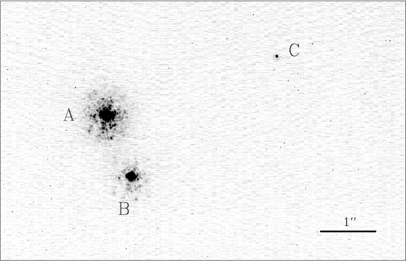
Figure 1: Portion of a raw image of KIC 4150611, taken on 2014-07-07 with the NIRC2 camera in the Hcont filter. Three point sources are clearly visible. Those marked by A and B are components of the well-known visual binary ADS 12310 AB. North is up, and East is left.

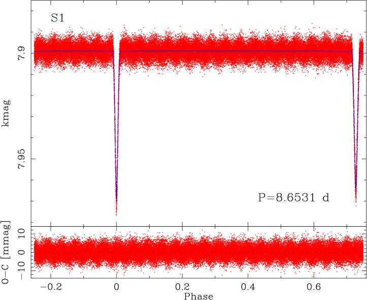
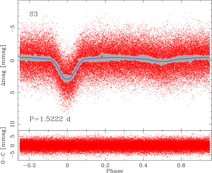
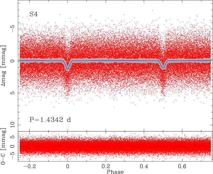
Figure 2: The S1 (top), S3 (middle), and S4 (bottom) light curves, representing three out of four periods of eclipses observed in the KIC 4150611 system. Red dots are the observations (S1) or residuals of previous fits cleaned from pulsations (S3 and S4). Grey symbols are bins of 200 points in phase domain. Blue lines are the JKTEBOP models. Please note the change of the spread of residuals of each fit (lower panels). The respective parameters are listed in Table 3.

Table 1: Basic literature information on KIC 4150611

Parameter	Value	Reference
$\alpha_{\mathrm{ICRS}}$ (J2000)	$19^{\mathrm{h}}18^{\mathrm{m}}58\aas@@fstack{s}209$	1
$\delta_{\mathrm{ICRS}}$ (J2000)	$+39^{\circ}16^{\prime}01\aas@@fstack{\prime\prime}687$	1
$\mu_{\alpha}$ (mas/yr)	$-6.949(35)$	1
$\mu_{\delta}$ (mas/yr)	$-5.962(38)$	1
$\varpi$ (mas)	7.73(46)	1
Sp. Type	F1 V mA9	2
Observed magnitudes:
$B$	8.29	3
$V$	8.00	3
Kepler	7.899	4
$J$	7.185(39)	5
$H$	7.029(38)	5
$K$	6.945(24)	5

References: (1) Gaia DR1 (Gaia Collaboration, 2016);
(2) Niemczura et al. (2015); (3) Simbad (Wenger et al., 2000); (4) Kepler Input Catalog; (5) 2MASS (Skrutskie et al., 2006)

Having the observed magnitudes of 7.899 in the Kepler band and 8.00 in Johnson’s $V$, the KIC 4150611 (a.k.a. KOI 3156, HD 181469, HIP 94924, ADS 12310 AB, WDS J19190+3916AB) is one of the brightest objects listed in the Kepler Eclipsing Binaries Catalog (KEBC; Prša et al., 2011; Slawson et al., 2011; Kirk et al., 2016). It is usually classified as having a late-A spectral type. Its basic properties are summarised in Table 1.

According to the Washington Double Star catalogue, (WDS; Mason et al., 2001), it is a visual binary, discovered by F. Struve (no particular reference is given). The WDS currently holds 20 position measurements, with first one dated back to 1831, and the last one taken in 2015. During this time, the separation between the components A and B changed from $\sim$1$\aas@@fstack{\prime\prime}$8 to $\sim$1$\aas@@fstack{\prime\prime}$12, and the position angle from $\sim$206^∘ to $\sim$203^∘.

The eclipses were first noted in the KEBC, where three periods are currently given: 1.5222786(19), 8.6530923(36) and 94.1982(7) d. The second value was first found in Prša et al. (2011), and is incorrectly attributed to the brighter component in the WDS. Additional eclipses were reported later by Slawson et al. (2011), and also by Orosz (2015). Multiple eclipse periods are first given by Rowe et al. (2015), who claim four values: 0.7611224(29), 1.4342003(58), 8.6530988(66), and 94.22454(40) d, which can be found in the Kepler Object of Interest (KOI) data base. The first one is obviously half of the 1.522 d value from KEBC, while the second one (1.434 d) does not appear there.

KIC 4150611 was first found to be a spectroscopic binary by Molenda-Żakowicz et al. (2011), but they acquired only three spectra, and did not relate the spectral lines to any particular component, nor gave the orbital solution. They were also the first to mention this object in relation to pulsations. Shortly after it was identified as containing a hybrid $\delta$ Sct/$\gamma$ Dor pulsator by Uytterhoeven et al. (2011). Shibahashi & Kurtz (2012) studied the $\delta$ Sct pulsations, and used their new Fourier-transform-based formalism to obtain a radial velocity (RV) curve of the pulsating component, with the orbital period of $94.09\pm 0.11$ d. Later, Balona (2014) reconstructed a somewhat different RV curve, with $P=94.3\pm 0.1$ d, using a different approach. Finally, Niemczura et al. (2015) performed spectral analysis and obtained atmospheric parameters of the pulsator, showing that it is a rapidly-rotating star ($v\sin(i)=128\pm 5$ km/s) of spectral type F1 V mA9 ($T_{eff}=7400\pm 100$ K).

2 Data and methodology

2.1 Keck II/NIRC2 adaptive optics imaging

Table 2: The log and results of Keck II/NIRC2 observations. We show the date, filters (combination of two wheels), total number of exposures ($N_{exp}$), integration time per exposure ($t_{int}$), and number of co-adds per exposure. In the lower part of the table we show angular separations ($\rho$) and position angles ($\theta$) of stars B and C relatively to A, and their magnitude differences.

MJD	Date	Filter	$N_{exp}$	$t_{int}$	Co-adds	PI
		combination		[s]
56458.61442	2013-06-15	PK50_1.5+Br$\gamma$	15	1.0	5	Marcy
56845.42700	2014-07-07	PK50_1.5+Kcont	6	12.5	25	Knutson
56845.43081		PK50_1.5+Jcont	6	12.5	50
56845.43408		PK50_1.5+Hcont	6	12.5	50
57643.28633a	2016-09-11	PK50_1.5+Kcont	5	12.5	25	Baranec
57677.24852	2016-10-15	PK50_1.5+Kcont	8b	30/60	30/60	Baranec
57677.25537		K+clear	3c	1.81/18.1	10/100
MJD	$\rho_{AB}$	$\theta_{AB}$	$\rho_{AC}$	$\theta_{AC}$	$\Delta mag_{AB}$	$\Delta mag_{AC}$
	[mas]	[∘]	[mas]	[∘]	[mag]	[mag]
56458.61442	1151.51(39)	203.279(16)	3279.7(3.8)	287.794(71)	1.087(5)	5.00(13)
56845.42700	1146.17(11)	203.503(12)	3266.48(33)	288.002(13)	1.104(5)	5.139(47)
56845.43081	1146.24(9)	203.509(13)	3267.28(67)	287.987(15)	1.368(7)	5.266(55)
56845.43408	1146.42(8)	203.515(11)	3267.47(69)	287.990(15)	1.133(7)	5.168(22)
57643.28633a	1131.76(20)	203.053(36)	3226(12)	287.862(47)	1.099(7)	5.3(2)
57677.24852	1134.30(22)	203.490(22)	3242.38(52)	288.284(20)	1.125(5)	5.180(30)
57677.25537	1134.67(39)	203.468(22)	3243.17(87)	288.290(26)	1.052(2)	5.053(34)

^a Observations with bad AO correction. Results were not used in the further analysis.
^b The first two frames are composed of 30 co-adds (1 s each), while the following six are composed of 60 co-adds (also 1 s).
^c The first frame is composed of 10 co-adds (0.181 s each), while the following two are composed of 100 co-adds (also 0.181 s).

In the Keck Observatory Archive (KOA) we have found high-angular-resolution images of KIC 4150611, obtained with the NIRC2 camera, which is fed by the natural guide star adaptive optics (NGS AO; Wizinowich et al., 2000) on the Keck II telescope. These observations were taken on 2013 June 15 (filter: Br$\gamma$; program ID: U078N2; PI: Marcy) and 2014 July 07 (filters: Jcont, Hcont, Kcont; program ID: C191N2; PI: Knutson). We have supplemented these data with our own observations, performed on 2016 September 11 in the Kcont filter, and 2016 October 15 in filters Kcont and K. Unfortunately, on our first night the conditions were bad, which caused a poor AO correction. All observations were done in the “narrow” mode, which gives the field of view of $\sim$10${}^{\prime}\times 10^{\prime}$. As usual for infra-red observations, dithering was performed in order to remove the flux of the sky in further processing. Table 2 shows the observing log for AO imaging.

Except for the Br$\gamma$ data, from the KOA we downloaded raw frames, and we reduced and analysed them by ourselves with a combination of IRAF and Python-based routines. Under IRAF we applied corrections for bad pixel, flat field, and sky flux. Because there are no master flats for the -cont filters available from the NIRC2 website, we took our own calibrations for Kcont and Hcont, while for the Jcont band we had to look in the KOA for appropriate calibrations. In case of Br$\gamma$ frames, we used the calibrated ones, available in KOA directly. All data were then corrected for distortion. This was done with a freely-available, dedicated Python script which was prepared to follow the prescription described in Yelda et al. (2010) and Service et al. (2016), and which utilizes distortion maps that are available on line. Note, that the maps for observations taken after 2015 April differ from those from before that date. Therefore we used different maps for the KOA (from 2013 and 2014) and our own data (2016).

The images show three point sources: two bright ones, the A and B components that form the visual binary ADS 12310 AB, and a faint one (C), located approximately 3 arcsec NW from the bright pair (Figure 1). This star was out of the field of view of some 2013 data, due to dithering. We rejected such frames from our analysis.

For all three sources we performed relative astro- and photometric measurements. The positions of stars on the chip ($x,y$) were measured by fitting a 2D Gaussian to the core of the star’s point spread function (PSF). They were then translated to distances along the chip’s axes in angular scale ($\Delta\hat{x}$,$\Delta\hat{y}$), and later, to relative angular separations and position angles ($\rho$, $\theta$). For this we used the pixel scale and rotation angle values given on the same website as the distortion script, coming from Yelda et al. (2010) and Service et al. (2016). They are: $9.952\pm 0.002$ mas/pix and $0\aas@@fstack{\circ}252\pm 0\aas@@fstack{\circ}009$ for data taken before, and $9.971\pm 0.004$ mas/pix and $0\aas@@fstack{\circ}262\pm 0\aas@@fstack{\circ}020$ for data taken after 2015 April. Please note that we did not de-rotate the images, only applied the correction to the measurements of $\theta$.

Finally, we applied corrections for the atmospheric refraction, using the method described in Hełminiak (2009), assuming monochromatic refraction at the effective wavelength of a given filter, and calculating the refractive index $n$ with the method of Mathar (2004, 2007). For the atmospheric conditions (outside temperature, air pressure and humidity) we either used the values listed in the headers of files downloaded from KOA, or (for our own observations) we checked them in the KOA Ancillary Weather Data service. These corrections were, however, smaller than the measurement errors.

The instrumental fluxes were also measured by fitting a 2D Gaussian, but the photometry was done on frames not corrected for distortion. To obtain the magnitude differences we simply translated the flux ratios using the standard formula $\Delta mag=-2.5\log(F_{2}/F_{1})$.

All individual measurements were averaged, and $rms/\sqrt{N_{exp}}$ was taken as the uncertainty. The results are shown in Table 2. Very large errors for 2016 September measurements are caused by poor AO correction. That night, the star C was extremely difficult to detect, therefore its measurements are highly uncertain, and we did not use them in the further analysis. Also, due to short integration times and narrow bandwidth of the filter, this star was barely detectable on the Br$\gamma$ images. These measurements also have relatively large error bars.

The main purpose of our own AO observations was: (1) to determine if the star C is gravitationally bound to the AB pair, and (2) if it shows eclipses. These are discussed in further sections of this paper.

2.2 Kepler photometry and light curve analysis

Table 3: Results of the JKTEBOP fit to the S1, S3, and S4 curves, and absolute magnitudes in the Kepler band.

Curve	S1	S3	S4
$P_{ecl}$ (d)	8.6530941(16)	1.43420486(12)	1.5222468(25)
$T_{0}$ (JD-2454900)	61.00508(17)	60.76059(7)	60.8799(14)
$e$	0.374(7)	0.0(fix)	0.0(fix)
$\omega$ (∘)	13.0(2.6)	—	—
$r_{1}$	0.0373(21)	0.328(18)	0.093(16)
$r_{2}$	0.0398(17)	0.212(38)	0.071(18)
$i$ (∘)	89.28(14)	88.5${}^{+0.5}_{-6.4}$	88.8${}^{+1.2}_{-2.6}$
$J$	0.943(42)	0.111(22)	0.934(16)
$L_{2}/L_{1}$	1.07(17)	0.046(26)	0.5${}^{+0.7}_{-0.3}$
$L_{3}/L_{tot}$	0.8579(45)	0.9936(9)	0.997(2)
$L_{1}/L_{tot}$	0.06865(61)	0.00612(87)	0.0020(14)
$L_{2}/L_{tot}$	0.07245(60)	0.00028(16)	0.0010${}_{-0.0008}^{+0.0011}$
$Kmag_{1}$ (mag)b	5.25(13)	7.87(20)	9.09(77)
$Kmag_{2}$ (mag)b	5.19(19)	11.22(62)	9.84${}^{-1.20}_{+0.88}$
$rms_{LC}$ (mmag)	3.13	2.30/0.21c	1.86/0.09c

^a From the periodogram analysis. ^b From the observed magnitude of the whole system (7.899 mag)
and Gaia DR1 distance ($129.4\pm 7.7$ pc). ^c For the unbinned and binned curve, respectively.

In this study we make use of the Q0-Q17 Kepler mission photometry, publicly available from the KEBC website. We used the de-trended relative flux measurements $f_{dtr}$, that were later transformed into magnitude difference $\Delta m=-2.5\log(f_{dtr})$, and finally the KEBC value of $k_{mag}$ was added. We call the resulting light curve (LC) the stage 0 (S0) curve. Due to the amount of data and limited computational resources, only long-cadence data were used in the LC analysis.

Before the light curve (LC) analysis, we filtered out the eclipses of the F1-type star, applying the following ephemerides: $2544840.707336+E\times 94.226$ d, which are slightly different than those given in the KEBC, but in agreement with Balona (2014) or Rowe et al. (2015). With this procedure we also removed several eclipses that occurred in the component B, and which coincided with the 94-day period. We called this resulting light curve the stage 1 (S1) curve. The main variability in this curve are the eclipses with 8.65-day period.

For all the LC fits we used version 28 (v28) of the code JKTEBOP (Southworth et al., 2004a, b), which is based on the EBOP program (Popper & Etzel, 1981). We fitted for the period $P$, primary (deeper) eclipse mid-time $T_{0}$, eccentricity $e$, periastron longitude $\omega$, inclination $i$, ratio of fluxes $L_{2}/L_{1}$, ratio of central surface brightnesses $J$, sum of the fractional radii $r_{1}+r_{2}$ (in units of major semi-axis $a$), their ratio $k$, and fractional amount of the third light $L_{3}/L_{tot}$. With several other sources of brightness variation (pulsations, additional eclipses), the S1 curve can be treated as affected by a correlated (red) noise. Therefore, for reliable error estimation, we applied the residual-shifts (RS) method. The best fit was done on the complete Q0-Q17 long-cadence light curve, but, due to amount of data, for the error estimation we worked on single-quarter LCs. Our approach is common for all Kepler targets from our program and is described in details in Hełminiak et al. (2016).

We first made the fit for the 8.65-day pair to the S1 curve, and run the RS to calculate the uncertainties for this system. We then took the residuals and run a Lomb-Scargle (LS) periodogram in order to identify additional periods.

We found a number of peaks related to pulsations, as well as a period of eclipses of 1.434205 d (see Sect. 3.5). We run the JKTEBOP once again with this period fixed, only to correct for these eclipses and improve the identification of frequencies of pulsation. The residuals of this intermediate JKTEBOP fit we call the stage 2 (S2) curve. We made another periodogram run on it, and we identified the most prominent pulsation periods (Sect. 3.1). We then removed the pulsations from the residuals of the S1 curve, and obtained the stage 3 (S3) curve, in which the main variability are the eclipses of the 1.43-day period. The final JKTEBOP fit for this period, the second one with proper error calculations, was done on the S3 curve. The residuals of this fit to S3 we call the stage 4 (S4) curve, in which we can see eclipses with the 1.52-day period. The last JKTEBOP run was done on the S4 curve.

Because the pulsations were mainly removed, the phase-folded S3 and S4 curves show a significantly smaller noise than the residuals of S1. We treated S3 and S4 as showing no correlated noise, and used a bootstrap approach to calculate the uncertainties.

We present the results of JKTEBOP fits to curves S1, S3, and S4 in Table 3 and Figure 2. Apart from the parameters given directly by JKTEBOP, we also calculated the fractional fluxes of each component and used them together with the apparent magnitude of the system to calculate individual apparent magnitudes in the Kepler band ($kmag$). Then, using the known distance, and assuming it is the same for all three pairs, we estimated the absolute ones ($Kmag$). The distance modulus is $Kmag-kmag=-5.56\pm 0.13$ mag. Zero extinction is assumed. The sum of the individual fractional fluxes also allows us to estimate the contribution from the remaining component A to be 84.95 per cent and its absolute magnitude $Kmag_{A}=2.52(13)$ mag (assuming that the total light in the Kepler LC comes only from seven stars: the pulsator and components of three shorter-period EBs).

2.3 HIDES spectroscopy and radial velocities

Figure 3: Cross-correlation function of KIC 4150611, from the spectrum taken on July 27, 2014. Two sharp peaks correspond to the G-type stars forming the 8.65-day binary (components Ba+Bb), the broad one is due to the F1-type star (component Aa). Velocities not shifted to the Solar system barycentre.

We observed the target as part of our program of spectroscopic monitoring of bright Kepler eclipsing binaries (Hełminiak et al., 2015, 2016, 2017). We used the 1.88-m telescope of the Okayama Astrophysical Observatory (OAO-1.88), with the HIgh-Dispersion Echelle Spectrograph (HIDES; Izumiura, 1999), fed through a 2$\aas@@fstack{\prime\prime}$7 diameter circular fibre (Kambe et al., 2013). Light from both visually separated components was collected. The instrument set-up, observational strategy, and spectroscopic data reduction scheme are described in details in Hełminiak et al. (2016).

Between July 2014 and October 2016, we obtained 17 high resolution ($R\sim 50000$) spectra. Despite four eclipsing periods were detected in Kepler data, velocities corresponding to only two of them could be measured – of a pair of G-type stars on a 8.65-day orbit, and of the F1-type pulsator on the 94.2-day orbit. The peculiar cross-correlation function (CCF) is shown in Figure 3. It is composed of two sharp peaks, that belong to the components of the G-type binary, and a very broad one, coming from the fast rotator of spectral type F1. This contaminator introduces additional systematic variation to the RV measurements of the other two components visible in spectra, and is the probable source of systematic uncertainties that dominate the error budget of their orbital fit.

For calculation of the RVs of the G-type pair we decided to use our own implementation of the TODCOR technique (Zucker & Mazeh, 1994), which finds velocities $v_{1}$ and $v_{2}$ of two stars simultaneously. Individual RV errors were estimated with a bootstrap approach (Hełminiak et al., 2012).

The RVs of the F1-type star (component A) were measured from the position of the $H_{\beta}$ line (4861.363 Å). We chose this line due to the fact that the Balmer series are the dominant features in the spectra, and $H_{\beta}$ lays in a spectral range that is significantly less affected by lines from the G-type pair and tellurics than, for example, $H_{\alpha}$. It is also in the centre of its echelle order, and the SNR around it is significantly higher than around lines at shorter wavelengths, like $H_{\gamma}$ or $H_{\delta}$. We measured its position by fitting a Gaussian to its core under IRAF’s task splot. As the measurement error, we assume a conservative value of 0.1 Å, which corresponds to $\sim$6 km/s at this wavelength. The orbital fit later showed that these errors were in fact overestimated.

2.4 RV orbital fits

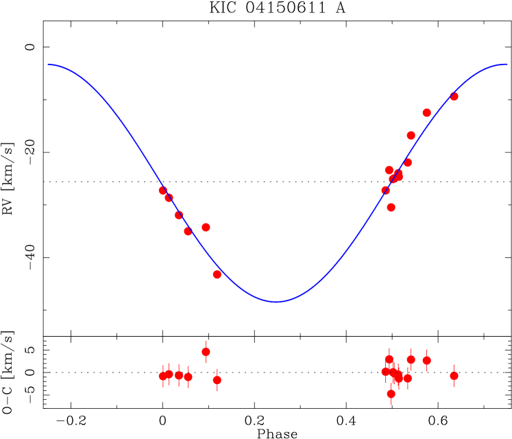
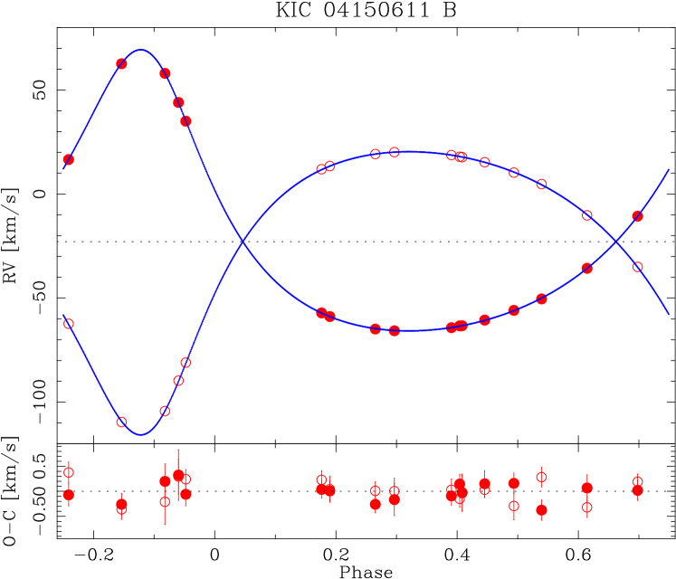
Figure 4: Radial velocity curves of the components A (left) and B (right) of KIC 4150611, phase folded with their orbital periods. The best-fitting models are plotted with blue lines. Filled circles on the right panel refer to the primary Ba, and open ones to the secondary Bb. Phases 0 are set for the eclipse mid-times (the deeper one in case of B).

Table 4: Results of the V2FIT fits to the RV measurements of the F1-type pulsator (component A), and the G-type pair (component B).

Parameter	Component A	Component B
Type of fit	SB1	SB2
$P$ (d)	94.226(fix)	8.6530941(fix)
$T_{p}$ (JD-2454900)	105.5(1.0)	60.0781(28)
$K_{1}$ (km/s)	22.6(2.2)	67.55(19)
$K_{2}$ (km/s)	—	68.04(21)
$e$	0.0(fix)	0.374(fix)
$\omega$ (∘)	—	12.91(17)
$\gamma$ (km/s)	-25.86(62)	-22.882(38)
$a_{1}\sin(i)$ (R⊙)	42.1(4.0)	10.714(32)
$a_{2}\sin(i)$ (R⊙)	—	10.792(34)
$f(m)$ (M⊙)	0.113(33)	—
$M_{1}\sin^{3}(i)$ (M⊙)	—	0.894(10)
$M_{2}\sin^{3}(i)$ (M⊙)	—	0.887(10)
$rms_{1}$ (km/s)	2.19	0.18
$rms_{1}$ (km/s)	—	0.23

The RV orbits were found with the code V2FIT (Konacki et al., 2010), which fits a single or double-keplerian orbit with a Levenberg-Marquardt algorithm. We performed two orbital fits to the measured RVs. First for the 8.65-day pair (component B), treated as a double-lined spectroscopic binary (SB2), and second for the F1-type pulsator on a 94.2-day orbit (component A) treated as a single-lined spectroscopic binary (SB1). In the SB2 fit we fixed the period and eccentricity to the values found with JKTEBOP. We fitted for velocity amplitudes ($K_{1},K_{2}$), longitude of pericentre ($\omega$), systemic velocity ($\gamma$), and moment of the pericentre passage ($T_{p}$). With V2FIT it is possible also to fit for the difference between systemic velocities of two components ($\gamma_{2}-\gamma_{1}$), but we initially found it undistinguishable from zero.

In the SB1 fit, we set the period to the value that we used to filter out the eclipses, 94.226 d, and also kept it fixed. When set free, the result was nearly the same, but did not reproduce the moments of eclipses very well. Other parameters were essentially the same in both cases. We also kept $e$ fixed, as it was initially found indifferent from zero; i.e. we found $e<0.17$. This agrees with Shibahashi & Kurtz (2012), who found it smaller than 0.12, and with Balona (2014), who gives the value of 0.043, which is undetectable in our data. Other parameters were essentially the same, no matter if $e$ was fixed, or fitted for. In the final fit, we were only looking for $K$, $\gamma$ and $T_{p}$, which for circular orbits is defined as the moment of the first quadrature (highest value of RV). The value of $\gamma$ in this case should be taken with some caution, as it depends on the exact reference wavelength that was used in RV measurement. This, however, has no impact on the velocity amplitude.

Results of both fits are summarised in Table 4. Observed and modelled RV curves are shown in Figure 4. Uncertainties were estimated with a bootstrap procedure, which properly accounts for possible systematics. The individual RV measurement errors were re-scaled, so the final reduced $\chi^{2}$ is close to 1.

2.5 Eclipse timing variations

Two of our LCs – the S3 and S4 curves – were also checked for the eclipse timing variations (ETVs). The 8.65-day eccentric binary (our S1 curve) has been analysed by Borkovits et al. (2016), who did not detect any significant signal.

We used the radio-pulsar-style approach, presented in Kozłowski et al. (2011). In this method, a template LC is created by fitting a trigonometric (harmonic) series to a complete set of photometric data. Then, the whole set of photometric data is divided to a number of subsets. Their number is arbitrary, but for this study we set it to 200. For each subset, the phase/time shift is found by fitting the template curve with a least-squares method. This approach is well suited for large photometric data sets, especially those obtained in a regular cadence, like from the Kepler satellite.

3 Results

3.1 The hybrid pulsator and its motion

Figure 5: Left: An LS periodogram of the residuals of the LC fit of KIC 4150611, with the second period of eclipses (1.43421 d) removed. Peaks representing $\delta$ Sct and $\gamma$ Dor pulsations of the component Aa are seen at frequencies $>$16 and $\sim$2.6 d^-1, respectively. Middle: Zoom on the frequencies around the highest peak of the $\gamma$ Dor pulsations. The arrow marks the 23-rd harmonic of the 8.65-d period (23/8.653094 d^-1). Right: Zoom on the frequencies corresponding to the rotation period. Their structure suggest differential rotation and/or that they come from two stars.

In the residuals of the first fit we see several periodicities, which are even clearer in the S2 curve. The most prominent are the $\delta$ Scuti type pulsations of the F1-type star (highest peak at 20.243 d^-1), also reported by Shibahashi & Kurtz (2012) and Balona (2014), and the $\gamma$ Dor type pulsations (highest peak at 2.6064 d^-1). The $\delta$ Sct and $\gamma$ Dor pulsations have similar amplitudes, and the star meets the criteria of being a hybrid pulsator (Bradley et al., 2015). The corresponding periodogram is presented in Figure 5. A zoom on the $\gamma$ Dor area reveals a peak that coincides with the 23-rd harmonic of the 8.65-days orbital period. This mode is clearly seen in the phase-folded S1 curve (Fig. 2; top), but it is rather a coincidence than a pulsation mode induced in one of the G-type stars during close periastron passages, as it takes place in “heartbeat” (HB) stars (Beck et al., 2014). No such oscillations have been observed in main sequence stars of this type, and in the HB stars they usually have a declining amplitude. The exact frequency $f_{23}=2.6578921$ 1/d correspondst to the period of 0.376238 d. Multiplied by 23, it gives 8.653474 d, which is close to but significantly different than $P_{B}=8.6530941(16)$ d. The S1 curve phase folded with the period of 8.653474 d looks much worse than with the best-fitting period.

Another small but clearly seen group of peaks can be found at frequencies around 0.185 d^-1, shown on a zoom in Fig. 5. They most likely come from rotation of one of the components (probably the pair B), and their complicated structure reveals that the rotation is differential, and/or that they may be coming from two stars.

Both Shibahashi & Kurtz (2012) and Balona (2014) used the pulsations to detect the orbital motion of the F1-type component with the 94.2-day period. They used different approaches, which resulted in different values of $a\sin(i)$ and the predicted velocity amplitude $K$. Shibahashi & Kurtz (2012) used the split of periodogram peaks of pulsation in the frequency domain, caused by the orbital motion, but Balona (2014) argues that such side-lobes of the main peaks may be obscured or distorted by other, independent pulsation modes of similar frequencies. He also notes that amplitude variations may also generate side lobes in the frequency domain, and decided to work with all frequencies, and look for time delay.

Closer inspection of both results is actually confusing. Shibahashi & Kurtz (2012) clearly miscalculated (or made a typo in) the values of $a_{1}\sin(i)$ from their Table 4, giving them close to 1.2 AU, while the value expected from their RV amplitudes ($K\simeq 23.5$ km/s) would be rather 0.2 AU. Similar value can be deduced from Figure 15 of Balona (2014), but in his Table 3, he gives $a_{1}\sin(i)=0.140$, and a (properly) corresponding $K=16.2$ km/s. This solution is in agreement with his measurements of pulsation time delay, presented later in Figure 16.

Thanks to our direct RV measurements, and the orbital solution (Table 4), we can clarify the situation. Our value of $K_{1}=22.6\pm 2.2$ km/s agrees better with the one of Shibahashi & Kurtz (2012), and the corresponding $a_{1}\sin(i)$ is almost exactly 0.2 AU ($0.196\pm 0.019$). The value that can be deduced from Balona’s Figure 15 is therefore correct.

3.2 Astrometry of the AB pair

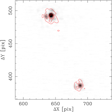
Figure 6: Portion of distortion-corrected images in Br$\gamma$ from 2013-06-15 (halftone) and Kcont from 2016-10-15 (red contours). Images are shifted to match positions of the component B. The centres of the component’s A PSF are misplaced by $\sim$2 pix (nearly 20 mas, or 2.6 AU at the distance to the system).

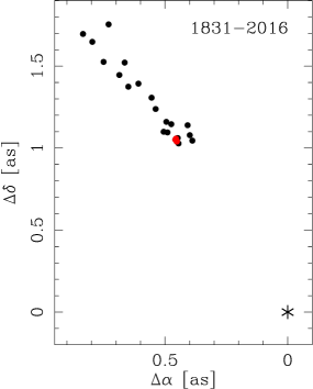
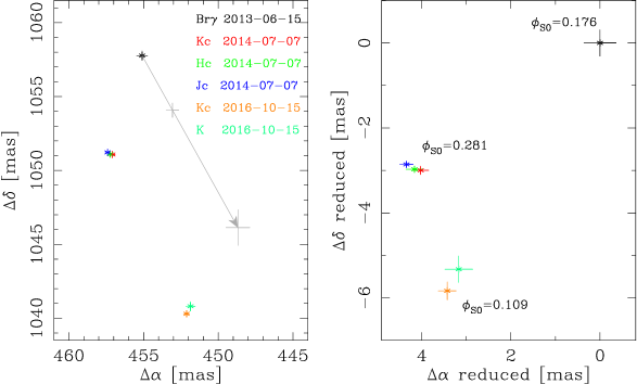
Figure 7: Astrometry of star A relatively to star B. Left: All data available from the WDS (black) and results from this work (red), on $\Delta\alpha/\Delta\delta$ plane, reconstructed from $\rho$ and $\theta$. The star B is set in (0,0) and marked with an asterisk. One can see a gradual movement with an average rate of 1.9(2) mas/yr and 3.5(3) mas/yr in $\alpha$ and $\delta$ respectively. Middle: Zoom onto our results, showing Keck II/NIRC2 observations (both archival and ours). Each measurement (date, filter) is denoted with a different colour. The grey arrow and crosses show the vector of the gradual orbital movement since 2013-06-15 and predicted relative positions in dates of other observations (with uncertainties). Right: Same measurements, but corrected for the gradual motion, and shifted, so the first Keck point is in (0,0). Labels $\phi_{S0}$ show phases of the 94.2-day orbit, according to the ephemeris used to clean the S0 curve from eclipses (Sect. 2.2). The data are clearly inconsistent with a $P=94.2$ d, $\hat{a}\simeq 1.55$ mas, $i\simeq 90^{\circ}$ orbit.

From the existence of eclipses with the 94.2-day period we know that the inclination of this orbit is close to $90^{\circ}$ ($\sin(i)\simeq 1$), so the true $a_{1}$ is close to 0.2 AU. At the distance to the system, this corresponds to the projected angular value of the major semi-axis $\hat{a}_{1}\simeq 1.55$ mas. This means that we can expect a peak-to-peak astrometric displacement of $\sim$3 mas of star A relatively to B, which should be measurable (Neuhäuser et al., 2007; Röll et al., 2008; Hełminiak et al., 2009, and the errors in Table 2). Comparison of two images, taken in 2013 and 2016, presented on the Figure 6, shows that we see a real relative motion between the two stars. The difference of $\sim$20 mas ($\sim$2.6 AU) can not be explained by the improper distortion correction (this would increase individual errors), nor the atmospheric refraction (measurements from observations in different filters from the same night are in agreement, the scale of refraction is much smaller).

In Figure 7 we show the measurements of the position of A relatively to B on the $\Delta\alpha/\Delta\delta$ plane. The left panel shows all data available from the WDS (starting from year 1831). Unfortunately the uncertainties are not given or can not be estimated in most cases. Nevertheless, one can easily note that in 185 years the two stars approached each other, moving with the average speed of 5.26(56)$\times$10^-3 mas/d or 1.9(2) mas/yr in $\alpha$, and 9.55(95)$\times$10^-3 mas/d or 3.5(3) mas/yr in $\delta$. This seems to be the orbital motion, as the measured proper motion is over 2 times larger. One can deduce that in $\sim$200 yr the two stars will pass very close to each other. The orbital period is most likely of the order of single thousands of years. Assuming $P_{AB}\sim 1000$ yr, and taking the estimates of total masses of A and B ($m_{AB,tot}\simeq 4.32$ M_⊙; see next Sections), we can estimate the physical major semi-axis to be $\sim$165 AU, or $\sim$1.28 asec in angular units, at the distance to the system ($129.4\pm 7.7$ pc). This suggests a high-inclination orbit and/or significant eccentricity.

The middle panel of Fig. 7 depicts only our Keck II/NIRC2 astrometry of star A relatively to B. The orbital displacement, predicted for the time span of observations, is plotted over. One can see that the measurements do not lay on the orbital motion path, and their spread is much larger than 3 mas (predicted for the 94.2-day orbit). The orbital motion seems to be dominant here, therefore, in the right panel of the same Figure, we show our measurements corrected for the orbital motion, and shifted to have the first point in (0,0). The spread of the data is still larger than 3 mas, and the points still do not lay along a single line, which would be expected for $i\simeq 90^{\circ}$. Moreover, when orbital phases are calculated (from the ephemeris given in Sect. 2.2), it turns out that all Keck observations were done in phases 0.1$-$0.3 (as labelled). If only the 94.2-day orbit was responsible for the observed positions, one would expect all the measurements to be well within $\sim$1.5 mas. A possible explanation is another body orbiting one of the components, but it is impossible to say which one, from the relative astrometry alone. It is difficult to estimate the parameters of the putative orbit, because the orientation of the one with $P=94.2$ d is unknown, and we only have precise measurements from three epochs. More high-precision astrometric data, from AO or interferometric, are needed to properly model all possible orbits. One should also keep in mind, that the long-term, gradual motion of A relatively to B (or vice versa) that we found from archival data, is quite uncertain. The archival astrometry from the WDS is not precise enough, and in most cases the uncertainties are not available. Nevertheless, it shows that the relative position of B vs. A has not changed much for nearly two centuries, so our results can not be explained by different proper motion and/or parallax of the two components. We also do not see any significant variations in the RV residuals.

3.3 Absolute parameters of KIC 4150611 B

Table 5: Absolute parameters of the components of KIC 4150611 B.

Parameter	Value	$\pm$
$M_{Ba}$ (M⊙)	0.894	0.010
$M_{Bb}$ (M⊙)	0.888	0.010
$R_{Ba}$ (R⊙)	0.802	0.044
$R_{Bb}$ (R⊙)	0.856	0.038
$a$ (R⊙)	21.508	0.075
$\log(g_{Ba})$	4.581	0.048
$\log(g_{Bb})$	4.522	0.038
$v_{syn,Ba}$ (km/s)a	4.69	0.26
$v_{syn,Bb}$ (km/s)a	5.00	0.20
$\tau_{syn}$ (Myr)b	56.51	0.24
$\tau_{cir}$ (Gyr)b	31.21	0.09

^a Rotation velocities, under the assumption of pseudo-synchronisation. ^b Time scales of spin-orbit synchronisation, and circulation of the orbit.

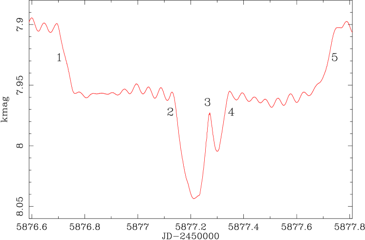
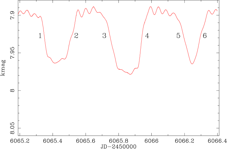
Figure 8: Examples of two kinds of eclipses of the F1-type pulsator. Left: A “deep” eclipse. One star transits the pulsator between moments 1 and 5, while the other only from 2 to 4. They eclipse each other in 3. Right: A triple eclipse. One star transits the pulsator between moments 1 and 2, and later between 5 and 6. The other star transits between 3 and 4. The wave-like modulation comes from pulsations. Note the same vertical scale on both panels. The exact depths vary slightly from one event to the other. Short-cadence data are shown.

Absolute values of stellar parameters of the components of the 8.65-day pair were calculated with the JKTABSDIM procedure, available together with the JKTEBOP. This simple code combines several spectroscopic and LC parameters (i.e.: $P,K_{1,2},i,e,r_{1,2}$) to derive a set of stellar absolute dimensions ($M_{1,2},R_{1,2},a$), and related quantities ($v_{syn1,2},\log(g_{1,2})$). Using formalism of the theory of tidal interactions, it also predicts the time scales of spin-orbit synchronisation ($\tau_{syn}$), and circularisation of the orbit ($\tau_{cir}$). If desired, the JKTABSDIM also calculates radiative properties ($L_{1,2}/L_{\odot},M_{bol1,2}$) and distance, but requires both effective temperatures, multi-colour photometry, and $E(B-V)$ as input. Due to lack of such data, we did not attempt to estimate the distance, but instead rely on the Gaia parallax (Gaia Collaboration, 2016).

The parameters are presented in Table 5. Indices ‘$Ba$’ and ‘$Bb$’ are used instead of ‘1’ and ‘2’. We reached $\sim$1.1 per cent precision in masses, and 4.6-5.5 per cent precision in radii. The latter is hampered by additional photometric variability in the system, presence of the (dominant) third light, and the fact that in JKTEBOP analysis we did not use spectroscopic flux ratios, which help to constrain the ratio of the radii. From the parameters from Tables 4, 3, and 5, one can see that the components of the studied pair are nearly identical, both being smaller, and slightly less massive than the Sun, and the more massive component (here, the primary Ba) seems to be smaller. All the important ratios – mass, radii, and fractional fluxes – agree with unity within errors. The contribution to the total system’s flux from this binary is 14.12(45) per cent, with 6.86(6) and 7.25(6) per cent individual contributions from the primary and secondary, respectively.

3.4 The 94.2 and 1.52-day periods.

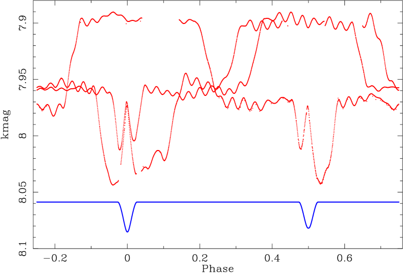
Figure 9: Three “deep” eclipses of the F1-type pulsator (red points, short-cadence data) phase folded with the period of the 1.52-day pair. The model curve of this pair is shown in blue (scaled and shifted for clarity). The brightening events in the “deep” eclipses coincide with the eclipses of the 1.52-day par, proving that this is the system revolving around the pulsator.

In Section 3.1 we discussed the orbital motion of the component A (F1-type pulsator) with the 94.2-day period. As it was mentioned before, the related eclipses have quite peculiar shapes, which is due to the binary character of the object revolving around this star. Those eclipses come in two shapes: “triple” with three small dips, or “deep” with one long drop in brightness, which deepens in its central part. Examples of a “triple” and a “deep” eclipse are shown in Figure 8.

The “triple” eclipse occurs when one star passes quickly in front of the pulsator, then is followed by a transit of the other star, and again by a passage of the first one, which this time is moving in the opposite direction. In the “deep” event, the first star starts to transit the pulsator, but the change of the observed direction (due to its orbital motion) occurs when it is still in front of the pulsator, therefore this transit is relatively long. During this eclipse the second star also transits the pulsator, which is the cause of the deeper part of the event, when larger area of the eclipsed component is obscured. Note also that during this deeper part there is a small brightening. It happens when the two transiting stars eclipse each other, and the obscured area of the star behind them is smaller. It is therefore easy to associate these brightening events with eclipses that occur with one of the other periods. They coincide with the 1.52-day period (see curve S4), meaning that this is the eclipsing pair that revolves around the F1-type star on the 94.2-day orbit. Figure 9 shows three “deep” eclipses (short-cadence data) phase-folded with the ephemeris for the S4 curve from Table 3. The brightenings occur exactly at phases 0.0 and 0.5.

Since we have recorded the orbital motion of the pulsator, we also attempted to do it for the 1.52-day pair, using the ETVs. This is however very difficult, as the eclipses are shallower than the $rms$ of the curve. The expected signal has the amplitude $A_{Ab}$ of the order of single minutes, but the errors of measurements themselves and their spread have larger values. Therefore we could not detect the signal securely, even though the period is known. We can only determine the detection limit of $A_{Ab}<283$ s ($rms$ of the ETVs), which translates into the limit of RV amplitude of the centre of mass $K_{Ab}<66$ km/s (from Eq. 8 in Hełminiak et al., 2016). Together with the RV amplitude of the pulsator itself ($K_{Aa}=22.6\pm 2.2$ km/s), we can determine the limit for ratio of masses: $q_{A}\equiv(M_{Ab1}+M_{Ab2})/M_{Aa}=K_{Aa}/K_{Ab}\ga 0.34$.

3.5 The 1.43-day period and the star C

Figure 10: A piece of the LS periodogram of the residuals of the JKTEBOP fit to the S1 curve around the value of 1.5222786 d, as given in the KEBC (marked with dashed vertical line). Instead of this value, we found a peak at 1.43420486 d. The LC phase-folded with this period (and cleared from pulsations) is the S3 curve (middle panel of Fig. 2).

The last period, not discussed so far, is the 1.4342 d, which is the period of the most prominent brightness variation in the S3 curve (Fig. 2). Because it was not listed in the KEBC, we were not aware of its existence, until we run the periodogram on the residuals of the JKTEBOP fit to the S1 curve. We were looking for the 1.52-day period, instead we noted the peak at $\sim$1.43 (Figure 10).

It is difficult to associate it with any of the two bright visual components. The Kepler pixel mask of the target is elongated and relatively large (due to the brightness), therefore covers several nearby faint stars, but changes from quarter to quarter and the common area is small. Because the eclipses are seen in all quarters, the source must be close to the bright visual pair. Therefore we suspect that the third star seen in the AO images is also an eclipsing binary, and 1.4342 d is its orbital period.

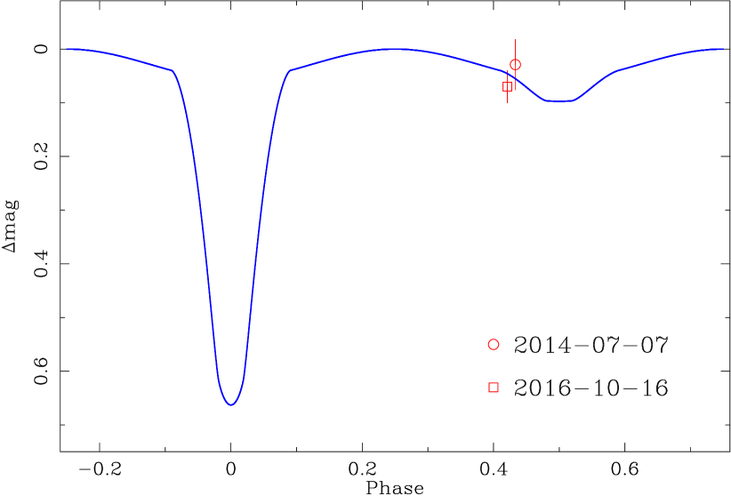
Figure 11: Photometric measurements of the star C, relatively to star A in Kcont (red symbols) as a function of the orbital phase of the S3 curve. Plotted over is the model S3 curve, corrected for the third light. The two measurements are shifted by 5.11 mag to match the model curve at the phases of observations. The unfortunate timing of the runs did not allow us to verify if the star C is the S3 eclipsing binary, even if the expected secondary eclipse is deeper in Kcont than in the Kepler band.

In order to confirm that, we performed photometric measurements on the archival and our own AO observations. We found out that the data from 2014 July 7 were taken during the beginning of the secondary eclipse, which helped us choose the observing set-up for our own observations. Before our run, we performed preliminary photometric measurements, and found that the lowest $rms$ is reached in Hcont and Kcont filters. We decided to observe in Kcont, using exactly the same settings as in 2014, because the expected brightness variation was larger than for Hcont (for eclipsing binaries composed of stars of significantly different $T_{eff}$, the longer the wavelength the deeper is the secondary eclipse). Additionally, in October we decided to observe the target also in the K (clear) filter. This set-up is more convenient and time efficient that the previous one, which includes a neutral density filter, and requires longer integrations and calibrations.

Unfortunately, the night of 2016-09-11, when the model predicted maximum brightness of the S3 curve, the conditions were too poor, and quality photometric measurements of the star C were impossible. To make matters worse, the orbital phase during the other night (2016-10-15) was almost exactly the same as in 2014, so no significant brightness variation is observed (Fig. 11). Therefore, with our current data, we can not confirm that the star C is the eclipsing pair with the period of 1.4342 d, but we can not exclude it either. Additional observations are required, and they should optimally be taken with the K+clear set-up.

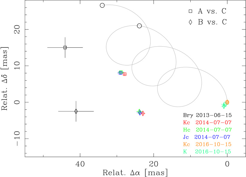
Figure 12: Astrometric measurements of stars A (squares) and B (diamonds) relatively to C. Measurements are shifted so that the one in Kcont from 2016 October is on (0,0). Each measurement (date, filter) is denoted with a different colour. The grey line shows the apparent motion on the sky over the course of the observations, expected from the parallax and proper motion values from Gaia DR1, and if the star C was a steady background object. Black circles mark the moments of archival observations (2013 June and 2014 July). These measurements show that the star C is probably not bound gravitationally with the AB pair, but may have a measurable proper motion. The difference in observed paths of stars A and B comes from their relative measurements, discussed in Sect. 3.1.

We also attempt to verify if the star C is bound to the AB system. In Figure 12 we show how the measured positions of stars A and B relatively to C change over time (grey line), assuming that C is a distant background object that has no measurable proper motion. Our measurements do not lay on the path predicted by the parallax and proper motion of KIC 4150611 from Gaia DR1, but they also do not agree with C being gravitationally bound to AB. We already discussed the possible systematics in Sect. 3.1. We conclude that C is most likely a background object, but has a measurable proper motion of few mas/year.

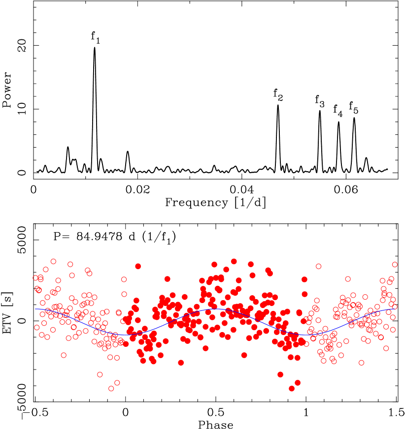
Figure 13: Top: An LS periodogram (in frequency domain) of the ETVs of the S3 curve. Five most prominent frequencies are marked. They were also detected by FREDEC. Bottom: The ETVs (red points) phase-folded with the period corresponding to the highest peak of the periodogram. The best-fitting sine function is plotted over (blue line). The data are repeated at phases $<0.0$ and $>1.0$ for clarity.

Table 6: Frequencies identified in the LS periodogram and by FREDEC in the ETVs of the S3 curve, including their false alarm probability (FAP) and ratios (last column). High-order ratios of $f_{3}:f_{1}$ and $f_{5}:f_{1}$ can be accidental and should be treated with caution.

$n$	$f_{n}$	$P_{n}=1/f_{n}$	FAP	$f_{n}:f_{1}$
	(1/d)	(d)
1	0.011771	84.9478	1.79$\times 10^{-8}$	1:1
2	0.046988	21.2818	2.02$\times 10^{-6}$	$\sim$4:1
3	0.054928	18.2057	7.06$\times 10^{-5}$	$\sim$14:3
4	0.058641	17.0523	1.06$\times 10^{-4}$	$\sim$5:1
5	0.061626	16.2271	3.23$\times 10^{-4}$	$\sim$21:4

FREDEC FAP of the whole quintuple: 1.06$\times 10^{-4}$.

Finally, we have checked the ETVs of S3, obtained as described in Section 2.5. After removing 3 outliers, we run an LS periodogram on our 197 measurements. Their mean separation is $\sim$7.35 d, therefore we looked for periods longer than 14.7 days. We detected 5 candidate peaks, with the strongest one at $P\sim 85$ d. We immediately noticed that frequencies of at least two others are multiples of the strongest one. To confirm the significance of the set of frequencies we found, we run a multi-frequency periodogram with the FREquency DEComposer algorithm (FREDEC; Baluev, 2013a, b). We found that this combination of peaks is statistically significant, with all having false alarm probability below 0.05%. These results are presented in Table 6 and Figure 13.

In Fig. 13 we also show our ETVs phase-folded with the 85-day period, and the best-fitting sine function. Despite the large scatter, the modulation with the amplitude of 804$\pm$85 s is clearly seen, even if it is lower than the $rms$ of the fit (1281 s). The amplitudes of other periods are no larger than 500 s, and when fitted for, the $rms$ drops only to 1200 s. It is difficult to assess if these four frequencies are physically real, or just some sort of artefacts in the data. With current sampling, each subset of $\sim$7.35 d covers about 5 orbital periods of the EB. Given the observed depth (or shallowness) of the eclipses, this seems to be a feasibility limit of the method we used – individual ETV measurement errors are quite large already. With longer sampling (e.g. 100 subsets, 14.7 d mean cadence), the ETV errors are obviously smaller. The 85 d period is still very well visible, but the other four become shorter than the approximate Nyquist cut-off ($\sim$29.4 d) and their secure detection is impossible. We then treat only the longest period as realistic.

However, assuming so, and that the modulation is caused by another body orbiting the EB, the observed amplitude can be translated into an unrealistic value of the mass function $f(M)\simeq 77.5$ M_⊙. Such a configuration would be difficult to explain. Therefore, the ETVs we observe for the S3 curve are rather not caused by another body. They might possibly reflect a different phenomenon, occurring on one of the stars of the whole KIC 4150611 system, like evolution of spots, which we know exist on the Ba+Bb pair, because we see the rotational period in the periodogram in Fig. 5. They may also be a result of a systematic factor we did not take into account.

3.6 Comparison with isochrones

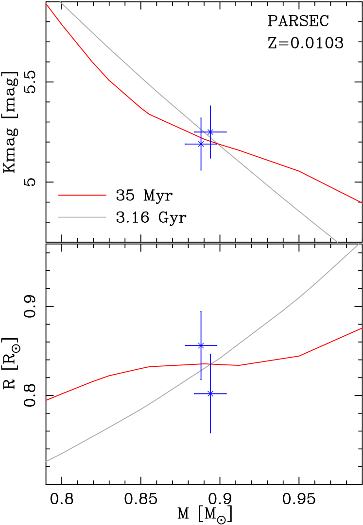
Figure 14: Comparison of our results for the G-type eclipsing pair with theoretical PARSEC $Z=0.0103$ isochrones on mass vs. absolute Kepler magnitude (top) and radius (bottom) planes. A good agreement is found for ages of 35 Myr (red line) and 3.16 Gyr (grey line). Stellar parameters predicted for the F1-type pulsator favour the former age.

We compare our results, i.e. masses, radii and absolute magnitude, with the theoretical PARSEC isochrones (Bressan et al., 2012), that include calculation of absolute magnitudes in the Kepler photometric band. The estimate of iron abundance from Niemczura et al. (2015) is $\log\epsilon(\mathrm{Fe})=7.33\pm 0.10$. Assuming the customary logarithmic abundances scale, with $\log\epsilon(\mathrm{H})=12$, and solar iron abundance of $\log\epsilon(\mathrm{Fe})_{\odot}=7.50\pm 0.04$ (Asplund et al., 2009), we get the value of $[Fe/H]=-0.17\pm-0.11$. We assume that this represents also the metallicity $[M/H]$ of KIC 4150611, and use PARSEC isochrones for this $[M/H]$ value, which translates into $Z\simeq 0.0103$ for this set.

Comparison of our results for Ba+Bb with the models on the $M/R$ and $M/Kmag$ planes shows a good agreement with the 35 Myr isochrone (Figure 14). For the estimated absolute magnitude of the pulsating star Aa ($2.52\pm 0.13$ mag), we can find its theoretical mass, radius, $\log(g)$, and temperature – 1.64(6) M_⊙, 1.376(13) R_⊙, 4.38(1) dex, and 8440(280) K, respectively. This is in disagreement with Niemczura et al. (2015), who give 3.8(2) dex and 7400(100) K, but it may be at least partially explained by uncertainties in the metallicity and age determinations, or the influence of additional flux on the spectral analysis. This may also be a hint for the existence of additional, relatively bright source in the system, i.e. that the pulsator constitutes less than $\sim$85 per cent of the total flux. In such situation the isochrone-predicted $T_{eff}$ would be lower.

Another relatively good fit is found for a 3.16 Gyr isochrone, but in such case the component Aa would be an F5-F6 type star ($5000<T_{eff}<6600$ K), and this is in strong disagreement with any spectral type estimation for this star. It would also have a mass of 1.32–1.36 M_⊙. We find this scenario to be unlikely for a $\delta$ Sct pulsator, and adopt 35 Myr as the age of the system.

Taking our isochrone-based estimation of the mass of the star Aa, and the mass function value derived from the RVs (0.113$\pm$0.033 M_⊙), we can estimate that the total mass of the Ab1+Ab2 pair is 0.90(13) M_⊙ (assuming $\sin^{3}(i)\simeq 1$). It is in a reasonable agreement with masses predicted by the isochrone from our $Kmag$ estimates, which are 0.44$\pm$0.13 and 0.32${}^{+0.21}_{-0.06}$ M_⊙ for the primary and secondary, respectively (total of 0.77${}^{+0.25}_{-0.14}$ M_⊙). The agreement would be slightly better if the component Aa was fainter (cooler and less massive), which may be another hint for an additional flux in the Kepler LC.

At the assumed age of 35 Myr, the PARSEC isochrone predicts that the Ab1+Ab2 pair would be still in pre-main-sequence stage, with radii of 0.61$\pm$0.09 and 0.52${}^{+0.14}_{-0.05}$ R_⊙. It is therefore plausible that this pair is still very active, and responsible for the relatively weak X-ray emission detected by ROSAT (Voges et al., 2000). Taking the isochrone-predicted masses and the orbital period 1.5222468(25) d, we can estimate the major semi-axis of the orbit: $a_{Ab}=5.11^{+0.55}_{-0.31}$ R_⊙. This leads to fractional radii of $r_{Ab1}=0.119_{-0.021}^{+0.019}$ and $r_{Ab2}=0.102^{+0.033}_{-0.017}$. They are in agreement with the results of the JKTEBOP fit to the S4 curve (Table 3). The ETV signal of this pair, produced by the orbital motion around the component Aa with $P=94.226$ d, would be $\sim$180-210 s, which is below our detection limit.

From the isochrones, we can also estimate effective temperatures of Ba and Bb, to be 5680 and 5640 K, respectively. This is consistent with the observed G spectral type. The age of 35 Myr suggests that this pair has not reached the state of pseudo-synchronisation yet. The theoretical time scale for its masses and period is $\tau_{syn}\simeq 57$ Myr (as calculated by JKTABSDIM). Therefore, the peaks in the periodogram at frequencies 0.18-0.19 d^-1 (Fig. 5) can be explained by a super-synchronous rotation of one or both components. In a pseudo-synchronous case, the frequency would be $\sim 0.11$ d^-1 ($P_{rot}\simeq 8.7$ d).

3.7 Galactic kinematics

To verify the young age of the system, we checked its Galactic velocity. Using the known parallax and proper motion (Tab. 1) and our value of the systemic velocity $v_{\gamma}$ for the component B (the more reliable one, we have calculated the spatial motion components: $U=2.52\pm 0.28$, $V=-23.29\pm 0.16$ and $W=-2.49\pm 0.13$ km/s (no correction for the solar movement has been done). These values put KIC 4150611 well within the thin disk, probably in a moving group called Coma Berenices or “local” (Nordström et al., 2004; Famaey et al., 2005; Seabroke & Gilmore, 2007). Famaey et al. (2005) have shown that ages of stars from this group vary from several to few hundreds of Myr. This confirms our “young” isochrone age of 35 Myr, and makes the “old” one (3.16 Gyr) even less probable.

4 Summary and future prospects

Figure 15: A mobile diagram showing the structure of the KIC 4150611 multiple system. The secure quintuple configuration is drawn with solid lines, orbital periods and spectral types (or their estimates) are shown. Our uncertainty of the character and membership of source C to the system is represented by dotted lines and question marks on its branch. The putative additional body on an orbit around either star A or B, discussed in Sect. 3.2, is not shown.

In Figure 15 we present the configuration of the multiple system KIC 4150611. The orbital periods and spectral types (at the “ends” of each branch) are given to the best of our knowledge. The uncertain character of the source C is taken into account. The additional body that could explain the AB pair astrometric measurements (Sect. 3.2) is not shown.

By analysing the eclipses seen in the Kepler light curve, HIDES radial velocities and AO observations from the Keck II telescope, we obtained a consistent image of a bright, interesting multiple system KIC 4150611. We managed to directly measure physical parameters of two of the components (Ba and Bb), which allowed us to find that this is a relatively young system. From its age we inferred properties of three other component (Aa, Ab1 and Ab2). Our results are still incomplete though.

Detailed analysis of the currently available data still leaves some open questions:

1. What is the 1.43-d eclipsing binary?

   The faint star C seems to be a good candidate, but we can not confirm it. We lack photometry taken during the primary (deep) eclipse. Sufficient observations do not have to be made with AO facilities, but good seeing conditions and a relatively large mirror is necessary to resolve the star from the AB pair, and obtain sufficient SNR of the target. If the star C is not the 1.43-d eclipsing binary, then another source must exist in the vicinity of the AB pair.

2. What is the proper motion of the system?

   The star C seems to be a distant background object, so a good reference point for astrometric measurements of the AB pair, but our measurements do not match the Gaia DR1 results. The faintness of C suggests a large distance, so a very slow proper motion would be expected. The discrepancy may be caused by an incorrect determination of $\mu_{\alpha}$ and $\mu_{\delta}$. Hopefully, this will be clarified with future data releases from Gaia.

3. Where does the 85-day period in ETVs come from?

   The signal in our ETVs of the 1.43-d binary is clear and statistically significant, but it leads to an improbable physical configuration (very high mass function). It is thus not clear if this modulation is an artefact, or has a physical origin, like evolution of spots. Confirmation would come from further timing measurements, but the source has to be resolved from the bright components A and B. This will only be possible if the star C is the 1.43-d binary. Other periods we found in the ETVs also require confirmation.

4. What is the true number of components?

   We presented several hints suggesting that another body may exist in the system. First, the isochrone-predicted properties (like temperature of Aa or masses of Ab1+Ab2) would be more consistent with observational constraints if the pulsator was fainter than what we found from our JKTEBOP fits. Second, as mentioned above, the 1.43-day period may not originate from the (seemingly unrelated) star C. Finally, our relative astrometry of A and B show a motion that can not be explained with the 94.2-day orbit. To verify this, more quality AO observations are required, including coronagraphic images of the surroundings of stars A and B. Precise ($\sim$1 mas level) astrometry from speckle observations, and optical or infra-red interferometers, is also welcome. Confirmation of the existence of another body would make KIC 4150611 a sextuple, or, still possibly, a septuple, which would be only the third known case.

Intriguing is the fact that in the system we see four periods of eclipses, with at least three coming from the system itself. The triple sub-system A may have two co-planar or nearly co-planar orbits (94.2 and 1.52 days), as it is observed in other objects with similar architecture, e.g. KOI-126 (Carter et al., 2011), HD 181068 (Derekas et al., 2011; Borkovits et al., 2012), or KIC 2856960 (Lee et al., 2013). The pairs with other two periodicities (8.65 and 1.43 days) do not, however, need to share the same orientation. Their inclinations are only calculated relatively to the plane of the sky, so the true orientations of their orbital angular momenta can still be very different. Astrometric detection of the 94.2-d motion, and complete modelling of the orbits and eclipses in the component A, will give valuable information about the distribution of momenta in this sub-system, giving important insight into the history of formation of this (young!) object.

KIC 4150611 is one of the most interesting astrophysical discoveries of the Kepler mission, and we believe it deserves further attention. Additional insight into the evolutionary status and structure of the Aa component may come from detailed asteroseismic studies of its pulsations. Please note that Shibahashi & Kurtz (2012) and Balona (2014) focus only on its orbital motion, and use only the $\delta$ Sct pulsations, while Uytterhoeven et al. (2011) only give the classification as a hybrid. A proper asteroseismic study is still missing.

We would also like to encourage the community to perform new AO observations, in order to answer the questions described above.

Appendix A RV measurements

In Table 7 we present single measurements of RVs of components Aa, Ba, and Bb. For Aa, for every observation, we initially assumed equal uncertainties of 6 km/s. For Ba and Bb they were obtained from our TODCOR runs. Final measurement uncertainties $\epsilon$, given in the Table, are scaled to have the reduced $\chi^{2}$ of the fit close to 1.

Table 7: Radial velocity measurements used in this work.

HJD	$v_{Aa}$	$\epsilon_{Aa}$	$(O-C)_{Aa}$	$v_{Ba}$	$\epsilon_{Ba}$	$(O-C)_{Ba}$	$v_{Bb}$	$\epsilon_{Bb}$	$(O-C)_{Bb}$
-2450000	(km/s)	(km/s)	(km/s)	(km/s)	(km/s)	(km/s)	(km/s)	(km/s)	(km/s)
6866.212043	-23.37	2.34	2.92	-57.133	0.168	0.038	11.881	0.182	0.231
6866.979087	-25.09	2.34	0.05	-64.910	0.170	-0.260	19.199	0.180	0.010
6867.251395	-24.92	2.34	-0.19	-65.725	0.323	-0.165	20.110	0.258	0.004
6868.065963	-23.97	2.34	-0.47	-64.250	0.187	-0.092	18.723	0.215	0.031
6868.184130	-24.64	2.34	-1.31	-63.338	0.198	0.146	17.865	0.173	-0.148
6870.002952	-21.93	2.34	-1.30	-35.688	0.265	0.067	-10.252	0.201	-0.320
6913.990303	-27.24	2.34	-0.81	-10.650	0.202	0.019	-35.018	0.155	0.192
7062.376385	-12.46	2.34	2.67	62.588	0.215	-0.260	-109.603	0.201	-0.359
7111.244355	-34.25	2.34	4.59	-55.916	0.207	0.159	10.253	0.272	-0.294
7148.151220	-27.23	2.34	0.17	16.566	0.220	-0.073	-62.343	0.210	0.376
7302.007666	-43.21	2.34	-1.69	-50.414	0.203	-0.375	4.748	0.196	0.285
7526.176108	-30.46	2.34	-4.74	-60.580	0.268	0.151	15.270	0.157	0.032
7530.264186	-16.78	2.34	2.86	57.936	0.350	0.198	-104.312	0.447	-0.210
7539.110077	-9.35	2.34	-0.74	43.984	0.508	0.325	-89.638	0.345	0.294
7669.010773	-28.63	2.34	-0.38	34.977	0.230	-0.060	-81.013	0.198	0.240
7671.067542	-31.93	2.34	-0.63	-58.882	0.200	0.008	13.425	0.259	0.042
7672.956861	-35.00	2.34	-0.99	-63.287	0.369	-0.025	17.751	0.361	-0.038