Stability of stationary inverse transport equation in diffusion scaling

Ke Chen Mathematics Department, University of Wisconsin-Madison, 480 Lincoln Dr., Madison, WI 53705 USA. ke@math.wisc.edu Qin Li Mathematics Department, University of Wisconsin-Madison, 480 Lincoln Dr., Madison, WI 53705 USA. qinli@math.wisc.edu  and  Li Wang Department of Mathematics, Computational and Data-Enabled Science and Engineering Program, State University of New York at Buffalo, 244 Mathematics Building, Buffalo, NY 14206 USA. lwang46@buffalo.edu
Abstract.

We consider the inverse problem of reconstructing the optical parameters for stationary radiative transfer equation (RTE) from velocity-averaged measurement. The RTE often contains multiple scales characterized by the magnitude of a dimensionless parameter—the Knudsen number (𝖪𝗇𝖪𝗇\mathsf{Kn}). In the diffusive scaling (𝖪𝗇1much-less-than𝖪𝗇1\mathsf{Kn}\ll 1), the stationary RTE is well approximated by an elliptic equation in the forward setting. However, the inverse problem for the elliptic equation is acknowledged to be severely ill-posed as compared to the well-posedness of inverse transport equation, which raises the question of how uniqueness being lost as 𝖪𝗇0𝖪𝗇0\mathsf{Kn}\rightarrow 0. We tackle this problem by examining the stability of inverse problem with varying 𝖪𝗇𝖪𝗇\mathsf{Kn}. We show that, the discrepancy in two measurements is amplified in the reconstructed parameters at the order of 𝖪𝗇p(p=1 or2)superscript𝖪𝗇𝑝𝑝1 or2\mathsf{Kn}^{p}~{}(p=1\text{ or}~{}2), and as a result lead to ill-posedness in the zero limit of 𝖪𝗇𝖪𝗇\mathsf{Kn}. Our results apply to both continuous and discrete settings. Some numerical tests are performed in the end to validate these theoretical findings.

All three authors thank the two anonymous referees for the very careful reading of the paper. It leads to significant improvement. The work of K.C. and Q. L. is supported in part by a start-up fund of Q.L. from UW-Madison and National Science Foundation under the grant DMS-1619778. The work of L.W. is supported in part by a start-up fund from SUNY Buffalo and the National Science Foundation under the grant DMS-1620135.

1. Introduction

In this paper, we study the stability of inverse stationary radiative transfer equation (RTE) in different regimes. RTE is a stereotype kinetic equation that describes the dynamics of photon particles in materials with various optical properties [12]. The optical properties are characterized by two parameters—the scattering coefficient and absorption coefficient. Generally speaking, we denote f(x,v)𝑓𝑥𝑣f(x,v) the distribution of particles at location x𝑥x moving with velocity v𝑣v, and it obeys:

vxf=k(x,v,v)f(x,v)dvσ(x,v)f.𝑣subscript𝑥𝑓𝑘𝑥𝑣superscript𝑣𝑓𝑥superscript𝑣differential-dsuperscript𝑣𝜎𝑥𝑣𝑓v\cdot\nabla_{x}f=\int k(x,v,v^{\prime})f(x,v^{\prime})\mathrm{d}{v^{\prime}}-\sigma(x,v)f\,.

Here xΩd𝑥Ωsuperscript𝑑x\in\Omega\subset\mathbb{R}^{d} with d=2,3𝑑23d=2,3 depending on the dimension of the problem, and v𝕊d1𝑣superscript𝕊𝑑1v\in\mathbb{S}^{d-1}, the unit sphere in dsuperscript𝑑\mathbb{R}^{d}. It indicates that the particles move with fixed speed (unified to 111) and therefore has one fewer dimension than x𝑥x. k(x,v,v)𝑘𝑥𝑣superscript𝑣k(x,v,v^{\prime}) is termed the scattering coefficient, representing the probability of particles that move in direction vsuperscript𝑣v^{\prime} changing to direction v𝑣v. dvd𝑣\mathrm{d}{v} has the normalized unit measure. σ(x,v)𝜎𝑥𝑣\sigma(x,v) is the total absorption coefficient that represents certain amount of photon particles being absorbed and scattered by the material. The boundary condition is typically imposed as Dirichlet type. We separate the “out-going” and “in-coming” part of boundary by defining:

Γ±={(x,v):xΩ,±vnx>0},subscriptΓplus-or-minusconditional-set𝑥𝑣formulae-sequence𝑥Ωplus-or-minus𝑣subscript𝑛𝑥0\Gamma_{\pm}=\{(x,v):x\in\partial\Omega\,,\pm v\cdot n_{x}>0\}\,, (1)

where nxsubscript𝑛𝑥n_{x} is the normal direction pointing out of ΩΩ\Omega at point xΩ𝑥Ωx\in\partial\Omega. In this way, ΓsubscriptΓ\Gamma_{-} collects all boundary coordinates that represent particles coming into the domain where Γ+subscriptΓ\Gamma_{+} collects the opposite. It is on the first set we impose Dirichlet boundary condition:

f|Γ=ϕ(x,v).evaluated-at𝑓subscriptΓitalic-ϕ𝑥𝑣f|_{\Gamma_{-}}=\phi(x,v)\,. (2)

The well-posedness is summarized from [16] and the solution is proved to be unique with full Dirichlet data.

Although the investigation of RTE is already enormous and generally acknowledged to be well-understood a long time ago, the inverse stationary RTE still attracted lots of attention in the past decade. The new life of RTE lies in the booming of medical techniques and a vast of medical images that require mathematical interpretation. In diffuse optical tomography, for example, near infra-red light (NIR) are sent into biological tissues, and by measuring the outgoing photon current at the surfaces of the tissues, scientists expect to “invert” the problem for the optical properties of the tissue. Mathematically that means one adjusts the incoming data f|Γevaluated-at𝑓subscriptΓf|_{\Gamma_{-}}, and measure a certain form of the out-going data f|Γ+evaluated-at𝑓subscriptΓf|_{\Gamma_{+}} seeking for k(x,v,v)𝑘𝑥𝑣superscript𝑣k(x,v,v^{\prime}) and σ(x,v)𝜎𝑥𝑣\sigma(x,v). Technically it is equivalent to seek for scattering coefficient k(x,v,v)𝑘𝑥𝑣superscript𝑣k(x,v,v^{\prime}) and absorption coefficient defined as

σa(x,v)=σ(x,v)𝕊n1k(x,v,v)dv,subscript𝜎𝑎𝑥𝑣𝜎𝑥𝑣subscriptsuperscript𝕊𝑛1𝑘𝑥𝑣superscript𝑣differential-dsuperscript𝑣\sigma_{a}(x,v)=\sigma(x,v)-\int_{\mathbb{S}^{n-1}}k(x,v,v^{\prime})\mathrm{d}{v^{\prime}}\,, (3)

which represents the probability of particles being absorbed by the material only. A vast literature has addressed the problem from various perspectives. The well-posedness of the inverse problem in a generic setting with σa(x)subscript𝜎𝑎𝑥\sigma_{a}(x) independent of v𝑣v was addressed in a pioneering paper [15], and the uniqueness based on gauge-invarience when σa(x,v)subscript𝜎𝑎𝑥𝑣\sigma_{a}(x,v) presents v𝑣v dependence was shown in [31]. The idea was to decompose the albedo operator according to the singularities. Another approach is to linerize the equation before applying inverse Born series, and show the convergence of the series [26]. The results on the stability of the “inverse” dates back to [33] and was made systematic in [6, 7, 9]. Many papers concern the time-dependent case and the associated stability analysis has also been conducted [21, 30, 14], and also [5] for a review.

Aside from the analytical studies, various numerical techniques are explored accordingly. Numerical treatments could be separated into two categories depending on whether linearization is conducted, both on the original physical domain, or via Green’s function representation [25, 26]. Either way, the resulting numerical problem is typically not well-posed: it is either under-determined or over-determined. The ill-posedness may be inherited from the continuous problem or due, in part, to the lack of data in experiments. The latter reason induces a purely numerical problem that can often be handled via optimization along with some regularization technique. Examples include the standard L2subscript𝐿2L_{2} regularization [1] for the smallness, TV regularization [32] for the least variance, H1subscript𝐻1H_{1} norm for some regularity, and L1subscript𝐿1L_{1} regularization [28] for sparsity, or Tikhonov type on each element in the inverse Born series [26]. The optimization techniques are borrowed accordingly, and efficiency and memory cost for both the Jacobian-type method and the Gradient based method have been compared. The way to set the regularization coefficient, on the other hand, is usually guided by the tolerance on the error [18, 17] and convergence speed.

One very interesting phenomenon associated with inverse stationary transport equation is its connection to the diffusion limit. It has been longly known in the area [29, 2, 3] that the diffusion approximation could serve as a substitute under certain scaling, and instead of inverting the transport equation, one studies the Calderón-like problems. That is, recovering the diffusion and attenuation coefficients 1σs1subscript𝜎𝑠\frac{1}{\sigma_{s}} and σasubscript𝜎𝑎\sigma_{a} in the following equation

Cx(1σsxu)+σau=0,xΩformulae-sequence𝐶subscript𝑥1subscript𝜎𝑠subscript𝑥𝑢subscript𝜎𝑎𝑢0𝑥Ω-C\nabla_{x}\cdot\left(\frac{1}{\sigma_{s}}\nabla_{x}u\right)+\sigma_{a}u=0,\qquad x\in\Omega (4)

using the Dirichlet boundary condition u|Ωevaluated-at𝑢Ωu|_{\partial\Omega} and the measurement of flux at boundaries un|Ωevaluated-at𝑢𝑛Ω\frac{\partial u}{\partial n}|_{\partial\Omega}. Here σssubscript𝜎𝑠\sigma_{s} and σasubscript𝜎𝑎\sigma_{a} are parameters derived from σ𝜎\sigma and k𝑘k from the RTE equation and C𝐶C is a constant that only depends on the dimension. The ill-posedness of the Calderón problem has been shown [19, 20] and its failure in capturing RTE based phenomenon in some scenario has been demonstrated [3], or in a similar problem on diffusion approximation in recovering the doping profile in the Boltzmann-Poisson system [13].

Despite the popularity of both problems, to the best knowledge of the authors, there has not been much study on exploring the connections between the two [4]. Specifically, some questions need to be addressed, such as: when and to what extent can diffusion approximation be used for RTE-based inverse problem? Will such approximation affect the stability in the inverse problem? Considering one type is ill-posed while the other one is well-posed, what is lost when such approximation is performed? In this paper, we make a first attempt to tackle these questions. In particular, we adopt a linearized framework (detailed in the next section), and study the well-posedness and the stability issues when passing to the diffusion limit for three different scenarios: recovering absorption coefficient, and recovering scattering coefficient in both critical and subcritical cases. We would like to mention that there are works on the change of stability with respect to certain parameters in the equation. In [8, 10] the authors particularly studied the stability of the inversion with respect to the modulation frequency in time-harmonic setting, and found that the increasing of the frequency brings more details in the recovery. In [27] the authors studied the stability of recovering acoustic equation.

We emphasize that the current paper concentrates on the illposedness as the transport equation approaches the diffusion regime (losing the stability). Except one special example in 1D (Theorem 5), we assume injectivity in our results. This is not a bizarre assumption as injectivity is shown for the associated nonlinear version of the problem [15]. Indeed, injectivity and stability are two separate issues in inverse problem: the former one concerns the uniqueness in recovery whereas the latter measures the accuracy in recovery when small perturbation in measurement is allowed. In terms of the spectral theory, the injectivity requires that the spectrum is away from zero, and stability studies the whole span of the spectrum. While stability naturally being the next step after injectivity, it is not uncommon that stability can be studied by assuming injectivity. As pointed out in [5], stability is studied in the setting of isotropic source and angularly averaged measurements while the uniqueness is not available [9, 8, 10].

The rest of paper is organized as follows. We present some preliminaries in the next section, including the derivation of the diffusion equation from the RTE and the set-up of the inverse problem in full generality. Section 3 and 4 are devoted to the three scenarios described above respectively. In all three cases, we utilize the linearization approach, study the well-posedness of the problem in both regimes, and examine the change of stability while passing to the diffusion limit. We also introduce a distinguishability parameter to indicate the stability and we justify that the inverse problem becomes more and more indistinguishable in the diffusion limit. Numerical tests are exploited to demonstrate the statements on the properties.

2. Preliminaries

Some preliminaries are collected in this section. The first subsection demonstrates the derivation of the diffusion equation from the RTE in the forward problem and the second subsection sets up the inverse problem we study in a general framework. For the conciseness of the paper we assume σs(x)subscript𝜎𝑠𝑥\sigma_{s}(x) and σa(x)subscript𝜎𝑎𝑥\sigma_{a}(x) do not have v𝑣v dependence.

2.1. Diffusion limit

The diffusion limit sets in when scattering is strong and absorption is weak. The equation in the dimensionless form reads:

{vxf=1𝖪𝗇σsf𝖪𝗇σaf,f|Γ=ϕ(x,v),cases𝑣subscript𝑥𝑓1𝖪𝗇subscript𝜎𝑠𝑓𝖪𝗇subscript𝜎𝑎𝑓otherwiseevaluated-at𝑓subscriptΓitalic-ϕ𝑥𝑣otherwise\begin{cases}v\cdot\nabla_{x}f=\frac{1}{\mathsf{Kn}}\sigma_{s}\mathcal{L}f-\mathsf{Kn}\sigma_{a}f\,,\\ f|_{\Gamma_{-}}=\phi(x,v)\,,\end{cases} (5)

where \mathcal{L} is the collision operator and in the velocity independent case it writes as:

f=f(x,v)dvf=ff.𝑓𝑓𝑥superscript𝑣differential-dsuperscript𝑣𝑓delimited-⟨⟩𝑓𝑓\mathcal{L}f=\int f(x,v^{\prime})\mathrm{d}{v^{\prime}}-f=\langle f\rangle-f\,. (6)

Here we have re-grouped the gain term and loss term in the collision for the ease of later presentation. A more general collision takes the form f=k(v,v)(f(x,v)f(x,v))dv𝑓𝑘superscript𝑣𝑣𝑓𝑥superscript𝑣𝑓𝑥𝑣differential-dsuperscript𝑣\mathcal{L}f=\int k(v^{\prime},v)(f(x,v^{\prime})-f(x,v))\mathrm{d}{v}^{\prime}, but our analysis in the rest of the paper can be easily adapted to this case. We therefore keep it in the simplest form, and assume that σssubscript𝜎𝑠\sigma_{s} has no v𝑣v dependence. There are two key features of the collision operator:

  • Mass conservation: [f]dv=0delimited-[]𝑓differential-d𝑣0\int\mathcal{L}[f]\mathrm{d}{v}=0. If we apply this property to the original equation, immediately we see that vfdv𝑣𝑓differential-d𝑣\int vf\mathrm{d}{v} is a divergence free field if σa=0subscript𝜎𝑎0\sigma_{a}=0;

  • One dimensional Null space: By setting [f]=0delimited-[]𝑓0\mathcal{L}[f]=0, one gets f=f𝑓delimited-⟨⟩𝑓f=\langle f\rangle, meaning that f𝑓f is a constant in velocity domain. We denote it as Null={ρ(x)}Null𝜌𝑥{\rm Null}\,\mathcal{L}=\{\rho(x)\}, the collection of functions that depend on x𝑥x only. This property is unique for RTE compared to other linear kinetic equation and it is the main reason that the asymptotic limit only consist of a scalar equation instead of a system.

As 𝖪𝗇0𝖪𝗇0\mathsf{Kn}\to 0, the equation falls into the diffusion limit and we have the following theorem:

Theorem 1.

Suppose f𝑓f solves (5). As 𝖪𝗇0𝖪𝗇0\mathsf{Kn}\to 0, f(x,v)𝑓𝑥𝑣f(x,v) converges to ρ(x)𝜌𝑥\rho(x), which solves the diffusion equation:

{Cx(1σsxρ)σaρ=0,ρ|Ω=ξf,cases𝐶subscript𝑥1subscript𝜎𝑠subscript𝑥𝜌subscript𝜎𝑎𝜌0otherwiseevaluated-at𝜌Ωsubscript𝜉𝑓otherwise\begin{cases}C\nabla_{x}\cdot\left(\frac{1}{\sigma_{s}}\nabla_{x}\rho\right)-\sigma_{a}\rho=0\,,\\ \rho|_{\partial\Omega}=\xi_{f}\,,\end{cases} (7)

Here C𝐶C is a constant depending on the dimension of the problem. The boundary condition is determined by:

ξf(x0)=fzl.subscript𝜉𝑓subscript𝑥0subscriptsuperscript𝑓𝑙𝑧\xi_{f}(x_{0})=f^{l}_{z\to\infty}\,.

with flsuperscript𝑓𝑙f^{l} solving

{vzzfl=σs[fl],z[0,)fl|z=0=ϕ(x0,v).casesformulae-sequencesubscript𝑣𝑧subscript𝑧superscript𝑓𝑙subscript𝜎𝑠delimited-[]superscript𝑓𝑙𝑧0otherwiseevaluated-atsuperscript𝑓𝑙𝑧0italic-ϕsubscript𝑥0𝑣otherwise\begin{cases}v_{z}\partial_{z}f^{l}=\sigma_{s}\mathcal{L}[f^{l}]\,,\quad z\in[0,\infty)\\ f^{l}|_{z=0}=\phi(x_{0},v)\,.\end{cases}
Proof.

The proof follows the standard asymptotic expansion with boundary layer analysis. In the zero limit of 𝖪𝗇𝖪𝗇\mathsf{Kn}, the distribution in the interior will stabilize whereas the boundary condition ϕitalic-ϕ\phi being away from the equilibrium function will prevent the solution converging near the boundary. To separate the two, we first expand the solution:

f(x,v)=fbd+fin,𝑓𝑥𝑣subscript𝑓bdsubscript𝑓inf(x,v)=f_{\text{bd}}+f_{\text{in}}\,, (8)

where fbdsubscript𝑓bdf_{\text{bd}} is the solution adjacent to boundary accounting for the boundary layer, while finsubscript𝑓inf_{\text{in}} characterizes the interior away from the layer. We study finsubscript𝑓inf_{\text{in}} first. As 𝖪𝗇0𝖪𝗇0\mathsf{Kn}\rightarrow 0, we apply the standard asymptotic expansion technique and write:

fin=f0+𝖪𝗇f1+𝖪𝗇2f2+.subscript𝑓insubscript𝑓0𝖪𝗇subscript𝑓1superscript𝖪𝗇2subscript𝑓2f_{\text{in}}=f_{0}+\mathsf{Kn}f_{1}+\mathsf{Kn}^{2}f_{2}+\cdots\,. (9)

Here we only consider the expansion away from the boundary layer so that fbdsubscript𝑓bdf_{\text{bd}} is negligible. Inserting the expansion in the equation (5) and equate like powers of 𝖪𝗇𝖪𝗇\mathsf{Kn}:

  • 𝒪(1)𝒪1\mathcal{O}(1)

    f0=0subscript𝑓00\mathcal{L}f_{0}=0. This immediately indicates that f0Nullsubscript𝑓0Nullf_{0}\in{\rm Null}\,\mathcal{L}. With the form given in (6), NullNull{\rm Null}\,\mathcal{L} consists functions that are constants in v𝑣v domain, and thus f0(x,v)=ρ(x)subscript𝑓0𝑥𝑣𝜌𝑥f_{0}(x,v)=\rho(x).

  • 𝒪(𝖪𝗇)𝒪𝖪𝗇\mathcal{O}(\mathsf{Kn})

    vxf0=σs[f1]𝑣subscript𝑥subscript𝑓0subscript𝜎𝑠delimited-[]subscript𝑓1v\cdot\nabla_{x}f_{0}=\sigma_{s}\mathcal{L}[f_{1}]. This indicates that f1=1(vxf0)subscript𝑓1superscript1𝑣subscript𝑥subscript𝑓0f_{1}=\mathcal{L}^{-1}\left(v\cdot\nabla_{x}f_{0}\right). \mathcal{L} is not a one-to-one map unless the domain is confined in NullNullsuperscriptperpendicular-to{\rm Null}\,\mathcal{L}^{\perp}, and the inverse on \mathcal{L} is pseudo-inverse. Considering the form of \mathcal{L} in (6), then Null={f:fdv=0}Nullsuperscriptperpendicular-toconditional-set𝑓𝑓differential-d𝑣0{\rm Null}\,\mathcal{L}^{\perp}=\{f:\int f\mathrm{d}{v}=0\}, and thus f1=vσsxρsubscript𝑓1𝑣subscript𝜎𝑠subscript𝑥𝜌f_{1}=-\frac{v}{\sigma_{s}}\cdot\nabla_{x}\rho.

  • 𝒪(𝖪𝗇2)𝒪superscript𝖪𝗇2\mathcal{O}(\mathsf{Kn}^{2})

    vxf1=σs[f2]σaf0𝑣subscript𝑥subscript𝑓1subscript𝜎𝑠delimited-[]subscript𝑓2subscript𝜎𝑎subscript𝑓0v\cdot\nabla_{x}f_{1}=\sigma_{s}\mathcal{L}[f_{2}]-\sigma_{a}f_{0}. Here we integrate the equation with respect to v𝑣v. The second term will vanish and the left hand side becomes:

    vx(vσsxρ)dv=σaρCx(1σsxρ)=σaρ.formulae-sequence𝑣subscript𝑥𝑣subscript𝜎𝑠subscript𝑥𝜌d𝑣subscript𝜎𝑎𝜌𝐶subscript𝑥1subscript𝜎𝑠subscript𝑥𝜌subscript𝜎𝑎𝜌\int v\cdot\nabla_{x}\left(-\frac{v}{\sigma_{s}}\cdot\nabla_{x}\rho\right)\mathrm{d}{v}=-\sigma_{a}\rho\quad\Rightarrow\quad C\nabla_{x}\cdot\left(\frac{1}{\sigma_{s}}\nabla_{x}\rho\right)=\sigma_{a}\rho\,. (10)

    Here the constant C𝐶C depends on the dimension of the velocity space.

Summarizing up the analysis we obtain fin(x,v)f0(x,v)=ρ(x)subscript𝑓in𝑥𝑣subscript𝑓0𝑥𝑣𝜌𝑥f_{\text{in}}(x,v)\to f_{0}(x,v)=\rho(x) that solves the diffusion equation (7).

We then need to provide ρ𝜌\rho a correct boundary condition and this comes from the treatment of fbdsubscript𝑓bdf_{\text{bd}}. For this we follow  [11]. At each point xΩ𝑥Ωx\in\partial\Omega, we perform tangential approximation and by stretching coordinates we can locally change the problem into a half space problem. More specifically, let x0Ωsubscript𝑥0Ωx_{0}\in\partial\Omega and nxsubscript𝑛𝑥n_{x} the normal direction pointing out of the domain, we denote z=nx(xx0)𝖪𝗇𝑧subscript𝑛𝑥𝑥subscript𝑥0𝖪𝗇z=-\frac{n_{x}\cdot(x-x_{0})}{\mathsf{Kn}}. For every fixed point x=x0nxy(y[0,))𝑥subscript𝑥0subscript𝑛𝑥𝑦𝑦0x=x_{0}-n_{x}y(y\in[0,\infty)) away from the layer along the ray pointing into the domain, z𝑧z\to\infty as 𝖪𝗇0𝖪𝗇0\mathsf{Kn}\to 0. After moving the coordinate frame to x0subscript𝑥0x_{0} with nxsubscript𝑛𝑥n_{x} direction, z=0𝑧0z=0 stands for boundary point and z=𝑧z=\infty is mapped to the interior. Then along z𝑧z direction the equation reads, in the leading order of 𝖪𝗇𝖪𝗇\mathsf{Kn}:

{vzzf=σs[f],z[0,)f|z=0=ϕ(x0,v).casesformulae-sequencesubscript𝑣𝑧subscript𝑧𝑓subscript𝜎𝑠delimited-[]𝑓𝑧0otherwiseevaluated-at𝑓𝑧0italic-ϕsubscript𝑥0𝑣otherwise\begin{cases}v_{z}\partial_{z}f=\sigma_{s}\mathcal{L}[f]\,,\quad z\in[0,\infty)\\ f|_{z=0}=\phi(x_{0},v)\,.\end{cases} (11)

It is a half space problem in z𝑧z with boundary condition given only at z=0𝑧0z=0. The problem is proved to have a unique solution and is computed in [23] and the infinite data on z𝑧z will be a constant in v𝑣v direction, which will be used to serve as the Dirichlet boundary condition for ρ𝜌\rho, meaning:

ρ(x0)=fz.𝜌subscript𝑥0subscript𝑓𝑧\rho(x_{0})=f_{z\to\infty}\,.

This is done at each grid point along the boundary and we end up with the boundary condition for xΩ𝑥Ωx\in\partial\Omega, denoted by ξf[ϕ](x)subscript𝜉𝑓delimited-[]italic-ϕ𝑥\xi_{f}[\phi](x) (or ξf(x)subscript𝜉𝑓𝑥\xi_{f}(x) for short). ∎

Remark 1.

The proof here is formal and is not specific on certain norm. In fact with general geometry and boundary condition it is believed to be correct but not proved yet. In 2-D physical domain and 1-D velocity sphere, due to the joint force of [34, 22], it can be made rigorous in L(dxdv)subscript𝐿d𝑥d𝑣L_{\infty}(\mathrm{d}{x}\mathrm{d}{v}) norm when boundary layer is excluded, meaning that as 𝖪𝗇0𝖪𝗇0\mathsf{Kn}\to 0:

fρL(dxidv)=𝒪(𝖪𝗇2/3)0,subscriptnorm𝑓𝜌subscript𝐿dsubscript𝑥𝑖d𝑣𝒪superscript𝖪𝗇230\|f-\rho\|_{L_{\infty}(\mathrm{d}{x_{i}}\mathrm{d}{v})}=\mathcal{O}(\mathsf{Kn}^{2/3})\to 0\,, (12)

and the decay from 𝒪(𝖪𝗇)𝒪𝖪𝗇\mathcal{O}(\mathsf{Kn}) to 𝒪(𝖪𝗇2/3)𝒪superscript𝖪𝗇23\mathcal{O}(\mathsf{Kn}^{2/3}) is mainly due to the curvature correction, which is controllably small but nontrivial. Here L(dxidv)subscript𝐿dsubscript𝑥𝑖d𝑣L_{\infty}(\mathrm{d}{x_{i}}\mathrm{d}{v}) stands for Lsubscript𝐿L_{\infty} norm in the interior only. We exclude a fixed small boundary layer of 𝒪(𝖪𝗇)𝒪𝖪𝗇\mathcal{O}(\mathsf{Kn}) width.

Remark 2.

Very frequently, RTE in 3D is simplified under some symmetry assumption. Specifically, we assume it with slab plan geometry. Denote x=(x1,x2,x3)Ω=2×(0,1)𝑥subscript𝑥1subscript𝑥2subscript𝑥3Ωsuperscript201x=(x_{1},x_{2},x_{3})\in\Omega=\mathbb{R}^{2}\times(0,1) and v=(sinθcosϕ,sinθsinϕ,cosθ)𝒮2𝑣𝜃italic-ϕ𝜃italic-ϕ𝜃superscript𝒮2v=(\sin\theta\cos\phi,\sin\theta\sin\phi,\cos\theta)\in\mathcal{S}^{2}, then we assume that all parameters and conditions are homogenized along x3subscript𝑥3x_{3} direction, i.e. σa(x)=σa(x3)subscript𝜎𝑎𝑥subscript𝜎𝑎subscript𝑥3\sigma_{a}(x)=\sigma_{a}(x_{3}), σs(x)=σs(x3)subscript𝜎𝑠𝑥subscript𝜎𝑠subscript𝑥3\sigma_{s}(x)=\sigma_{s}(x_{3}), and that boundary condition is ϕ(x,v)=ϕ(x3,cosθ)italic-ϕ𝑥𝑣italic-ϕsubscript𝑥3𝜃\phi(x,v)=\phi(x_{3},\cos\theta). The stationary RTE becomes:

vxf(x,v)=σs(x3)𝖪𝗇f(x,v)𝖪𝗇σa(x3)f(x,v)𝑣subscript𝑥𝑓𝑥𝑣subscript𝜎𝑠subscript𝑥3𝖪𝗇𝑓𝑥𝑣𝖪𝗇subscript𝜎𝑎subscript𝑥3𝑓𝑥𝑣\displaystyle v\cdot\nabla_{x}f(x,v)=\frac{\sigma_{s}(x_{3})}{\mathsf{Kn}}\mathcal{L}f(x,v)-\mathsf{Kn}\sigma_{a}(x_{3})f(x,v) (13)

with:

f(x,v)=14π0π02π[f(x,v)f(x,v)]sinθdϕdθ,𝑓𝑥𝑣14𝜋superscriptsubscript0𝜋superscriptsubscript02𝜋delimited-[]𝑓𝑥superscript𝑣𝑓𝑥𝑣superscript𝜃dsuperscriptitalic-ϕdsuperscript𝜃\mathcal{L}f(x,v)=\frac{1}{4\pi}\int_{0}^{\pi}\int_{0}^{2\pi}[f(x,v^{\prime})-f(x,v)]\sin\theta^{\prime}\mathrm{d}{\phi^{\prime}}\mathrm{d}{\theta^{\prime}}\,,

and the boundary condition f|Γ=ϕ(x3,cosθ)evaluated-at𝑓subscriptΓitalic-ϕsubscript𝑥3𝜃f|_{\Gamma_{-}}=\phi(x_{3},\cos\theta). With vx=cosθx3𝑣subscript𝑥𝜃subscriptsubscript𝑥3v\cdot\nabla_{x}=\cos\theta\partial_{x_{3}}, the stationary RTE becomes:

{cosθx3f(x3,cosθ)=σs(x3)𝖪𝗇(14π0π02π(f(x3,cosθ)f(x3,cosθ))sinθdϕdθ)𝖪𝗇σa(x3)f(x3,cosθ),f|Γ=ϕ(x3,cosθ).cases𝜃subscriptsubscript𝑥3𝑓subscript𝑥3𝜃subscript𝜎𝑠subscript𝑥3𝖪𝗇14𝜋superscriptsubscript0𝜋superscriptsubscript02𝜋𝑓subscript𝑥3superscript𝜃𝑓subscript𝑥3𝜃superscript𝜃dsuperscriptitalic-ϕdsuperscript𝜃𝖪𝗇subscript𝜎𝑎subscript𝑥3𝑓subscript𝑥3𝜃otherwiseevaluated-at𝑓subscriptΓitalic-ϕsubscript𝑥3𝜃otherwise\begin{cases}\cos\theta\partial_{x_{3}}f(x_{3},\cos\theta)=\frac{\sigma_{s}(x_{3})}{\mathsf{Kn}}(\frac{1}{4\pi}\int_{0}^{\pi}\int_{0}^{2\pi}(f(x_{3},\cos\theta^{\prime})-f(x_{3},\cos\theta))\sin\theta^{\prime}\mathrm{d}{\phi^{\prime}}\mathrm{d}{\theta^{\prime}})-\mathsf{Kn}\sigma_{a}(x_{3})f(x_{3},\cos\theta)\,,\\ f|_{\Gamma_{-}}=\phi(x_{3},\cos\theta)\,.\end{cases} (14)

For simplicity, we denote x=x3(0,1)𝑥subscript𝑥301x=x_{3}\in(0,1) and make change of variable v=cosθ(1,1)𝑣𝜃11v=\cos\theta\in(-1,1) to obtain:

{vxf(x,v)=σs(x)𝖪𝗇11f(x,v)f(x,v)dv2𝖪𝗇σa(x)f(x,v),(x,v)(0,1)×[1,1],f|Γ=ϕ(x,v),casesformulae-sequence𝑣subscript𝑥𝑓𝑥𝑣subscript𝜎𝑠𝑥𝖪𝗇superscriptsubscript11𝑓𝑥superscript𝑣𝑓𝑥𝑣dsuperscript𝑣2𝖪𝗇subscript𝜎𝑎𝑥𝑓𝑥𝑣𝑥𝑣0111otherwiseevaluated-at𝑓superscriptΓitalic-ϕ𝑥𝑣otherwise\begin{cases}v\partial_{x}f(x,v)=\frac{\sigma_{s}(x)}{\mathsf{Kn}}\int_{-1}^{1}f(x,v^{\prime})-f(x,v)\frac{\mathrm{d}{v^{\prime}}}{2}-\mathsf{Kn}\sigma_{a}(x)f(x,v)\,,\quad(x,v)\in(0,1)\times[-1,1]\,,\\ f|_{\Gamma^{-}}=\phi(x,v)\,,\end{cases} (15)

where v𝑣v is often termed as direction of flight. Sending 𝖪𝗇0𝖪𝗇0\mathsf{Kn}\to 0 and follow the same asymptotic derivation in the theorem above, one obtains C=13𝐶13C=\frac{1}{3} in the zero Knudsen number limit in (10). From here on, we always refer to equation (15) as the 1-D RTE. Notice here the velocity domain is interval [1,1]11[-1,1].

2.2. Inverse problem

The inverse problem can be set up associated with a map from the input data on one portion of the boundary to the measurement on the other portion. For RTE specifically, this map is often termed the albedo operator. Depending on the data-acquisition method in the experiments, the measurement can take various forms. Here we assume that only velocity-averaged measurement is available and define the measurement operator:

f(x)=Γ+(x)vn(x)f(x,v)dv,𝑓𝑥subscriptsubscriptΓ𝑥𝑣𝑛𝑥𝑓𝑥𝑣differential-d𝑣\mathcal{M}f(x)=\int_{\Gamma_{+}(x)}v\cdot n(x)f(x,v)\mathrm{d}{v}\,, (16)

where Γ+(x)subscriptΓ𝑥\Gamma_{+}(x) is the “outgoing” semisphere at x𝑥x defined in (1). And the albedo operator reads:

𝒜𝖪𝗇(σa,σs):ϕ|Γf,\mathcal{A}_{\mathsf{Kn}}(\sigma_{a},\sigma_{s})\,:\quad\phi|_{\Gamma_{-}}\rightarrow\mathcal{M}f\,, (17)

where ϕitalic-ϕ\phi is the Dirichlet boundary condition (2) and f(x)𝑓𝑥\mathcal{M}f(x) is the intensity of light propagating out of the domain at boundary point xΩ𝑥Ωx\in\partial\Omega. Then the inverse problem is to recover σasubscript𝜎𝑎\sigma_{a} and σssubscript𝜎𝑠\sigma_{s} given the information of the map 𝒜𝖪𝗇subscript𝒜𝖪𝗇\mathcal{A}_{\mathsf{Kn}}.

On the theoretical level, one concerns about the well-posedness and stability. The well-posedness problem states the following: given the full information on the map 𝒜𝒜\mathcal{A}, can one uniquely recover σasubscript𝜎𝑎\sigma_{a} and σssubscript𝜎𝑠\sigma_{s}? The answer is positive if a velocity-resolved measurement (i.e., f|Γ+evaluated-at𝑓subscriptΓf|_{\Gamma_{+}} for any v𝑣v instead of (17)) or time-dependent measurement is available [15, 31]. The analysis is based on singularity separation. Since the albedo operator is a forward map, an explicit form can be obtained and it consists of three parts, separated according to their singular level: the most singular part is a delta function that could be used to recover σasubscript𝜎𝑎\sigma_{a} through the inverse X-ray transform, and the secondly singular term is used to recover σssubscript𝜎𝑠\sigma_{s}, leaving the third term in Lsubscript𝐿L_{\infty}. The stability problem, on the other hand, asks: if the entire map is off from the accurate one by a small amount of error (𝒜𝒜~<ϵnorm𝒜~𝒜italic-ϵ\|\mathcal{A}-\tilde{\mathcal{A}}\|<\epsilon), how accurate the recovering could be? That is, will σaσ~anormsubscript𝜎𝑎subscript~𝜎𝑎\|\sigma_{a}-\tilde{\sigma}_{a}\| remain small? The problem is examined in [7, 6, 9] using the same kind of singular decomposition.

On the numerical level, the well-posedness problem takes a slightly different form: let σs,asubscript𝜎𝑠𝑎\sigma_{s,a} be discretized at Nxsubscript𝑁𝑥N_{x} grid points, then if for each incoming data ϕdsubscriptitalic-ϕ𝑑\phi_{d}, one could take Npsubscript𝑁𝑝N_{p} measurements at the boundary, how many incoming data is needed to fully recover σs,asubscript𝜎𝑠𝑎\sigma_{s,a}? This is intrinsically the same as in the theoretical level. The stability problem, however, has two sides. One is, assume that the data obtained is exact, how much error one obtains in recovering σs,asubscript𝜎𝑠𝑎\sigma_{s,a} if 𝖠𝖠\mathsf{A} gets perturbed a little. Here 𝖠𝖠\mathsf{A} is the matrix representation of 𝒜𝒜\mathcal{A}. This amounts to analyzing the condition number of the problem. Another is that if the measurement in (17) is off by some error, how accurate will σs,asubscript𝜎𝑠𝑎\sigma_{s,a} be? The answer to that lies in analyzing the norm of 𝖠1superscript𝖠1\mathsf{A}^{-1}. The first question is aligned with theoretical stability stated above, while the second question is a pure numerical issue. Concisely, since solving the inverse problem numerically often involves inverting a matrix (or a series of matrices in the nonlinear setting), even if the problem is well-posed, the numerical error is still hard to guarantee. All these questions are indirectly or partially resolved in many papers [2, 28].

We ask a different question in this paper. Our aim is to investigate the dependence of stability and condition number for the inverse problem on the Knudsen number. It is generally acknowledged that the inverse transport problem is well-posed (for most kinds of measurements and under mild assumptions on the scattering/absorption coefficients) whereas the inverse diffusion equation as a limit is ill-posed. Considering the two sets of equations are connected by simply passing to the 𝖪𝗇0𝖪𝗇0\mathsf{Kn}\to 0 limit, is there a more explicit explanation of the loss of uniqueness?

To answer this question, we adopt a linearization framework [28]. By assuming that the to-be-recovered coefficients σasubscript𝜎𝑎\sigma_{a} and σssubscript𝜎𝑠\sigma_{s} are only slightly deviated from some given functions from a priori knowledge, we linearize the transport equation around them and write down the relationship between the unknown parameters and the map 𝒜𝒜\mathcal{A}. As a result and as will be more clear later, we only need to invert a Fredholm operator of the first kind to recover those parameters. More importantly, this Fredholm operator reveals an explicit dependence on the Knudsen number, which allow us to analyze the stability of the inversion when varying the magnitude of 𝖪𝗇𝖪𝗇\mathsf{Kn}. We would also like to point out that the measurement we took in (17) contains minimum information that no uniqueness results on the reconstruction based on the singular decomposition are available. Nevertheless, the linearization approach we take allows us to quantify the stability explicitly in 𝖪𝗇𝖪𝗇\mathsf{Kn}, and is amenable for numerical schemes. Details will be provided along the paper.

As discussed before, depending on the assumptions on the media, different scenarios could take place. We present here three examples. The following sections are respectively devoted to recovering σasubscript𝜎𝑎\sigma_{a} when σssubscript𝜎𝑠\sigma_{s} is known, and recovering σssubscript𝜎𝑠\sigma_{s} in the critical (σa=0subscript𝜎𝑎0\sigma_{a}=0) and subcritical (σa>0subscript𝜎𝑎0\sigma_{a}>0) cases, respectively. It is not our aim in this paper to give a complete analysis for all scenarios but rather to investigate the problem for the first time and nail down the techniques that could make it possible.

3. Recover Absorption Coefficient σasubscript𝜎𝑎\sigma_{a}

3.1. Inverse problem set-up

In this section, we assume that the scattering coefficient is known (and we set it as σs=1subscript𝜎𝑠1\sigma_{s}=1 for simplicity), and recover the absorption coefficient σasubscript𝜎𝑎\sigma_{a}. The equation (5) reads:

{vxf=1𝖪𝗇f𝖪𝗇σaf,(x,v)Ω×𝕊,f|Γ=ϕ.cases𝑣subscript𝑥𝑓formulae-sequenceabsent1𝖪𝗇𝑓𝖪𝗇subscript𝜎𝑎𝑓𝑥𝑣Ω𝕊evaluated-at𝑓subscriptΓabsentitalic-ϕ\begin{cases}v\cdot\nabla_{x}f&=\frac{1}{\mathsf{Kn}}\mathcal{L}f-\mathsf{Kn}\sigma_{a}f,\qquad(x,v)\in\Omega\times\mathbb{S}\,,\\ f|_{\Gamma_{-}}&=\phi.\end{cases}\, (18)

Here ϕitalic-ϕ\phi is the inflow boundary condition and the solution is denoted by f(x,v;ϕ)𝑓𝑥𝑣italic-ϕf(x,v;\phi). Experimentally suppose one could measure data at one grid point yΩ𝑦Ωy\in\partial\Omega, then the mapping becomes:

𝒜(σa):ϕf().\mathcal{A}(\sigma_{a})\,:\quad\phi\to\mathcal{M}f(\cdot)\,.

We follow a linearization framework [28] and set a background absorbing coefficient σa0(x)subscript𝜎𝑎0𝑥\sigma_{a0}(x) by assuming that the residue

σ~a(x)=σa(x)σa0(x)subscript~𝜎𝑎𝑥subscript𝜎𝑎𝑥subscript𝜎𝑎0𝑥\tilde{\sigma}_{a}(x)=\sigma_{a}(x)-\sigma_{a0}(x)\,

is much smaller than σasubscript𝜎𝑎\sigma_{a}: σ~aσamuch-less-thannormsubscript~𝜎𝑎normsubscript𝜎𝑎\|\tilde{\sigma}_{a}\|\ll\|\sigma_{a}\|. Then the linearized problem with the same inflow boundary condition reads as

{vxf0=1𝖪𝗇f0𝖪𝗇σa0f0,f0|Γ=ϕ,cases𝑣subscript𝑥subscript𝑓01𝖪𝗇subscript𝑓0𝖪𝗇subscript𝜎𝑎0subscript𝑓0otherwiseevaluated-atsubscript𝑓0subscriptΓitalic-ϕotherwise\begin{cases}v\cdot\nabla_{x}f_{0}=\frac{1}{\mathsf{Kn}}\mathcal{L}f_{0}-\mathsf{Kn}\sigma_{a0}f_{0}\,,\\ f_{0}|_{\Gamma_{-}}=\phi\,,\end{cases}\, (19)

where f0(x,v;ϕ)subscript𝑓0𝑥𝑣italic-ϕf_{0}(x,v;\phi) is the function we linearize upon. Let

f~(x,v)=f(x,v)f0(x,v)~𝑓𝑥𝑣𝑓𝑥𝑣subscript𝑓0𝑥𝑣\tilde{f}(x,v)=f(x,v)-f_{0}(x,v)

be the fluctuation, then it solves the following equation by subtracting (19) from (18)

{vxf~=1𝖪𝗇f~𝖪𝗇σa0f~𝖪𝗇σ~af0,f~|Γ=0,cases𝑣subscript𝑥~𝑓1𝖪𝗇~𝑓𝖪𝗇subscript𝜎𝑎0~𝑓𝖪𝗇subscript~𝜎𝑎subscript𝑓0otherwiseevaluated-at~𝑓subscriptΓ0otherwise\begin{cases}v\cdot\nabla_{x}\tilde{f}=\frac{1}{\mathsf{Kn}}\mathcal{L}\tilde{f}-\mathsf{Kn}\sigma_{a0}\tilde{f}-\mathsf{Kn}\tilde{\sigma}_{a}f_{0}\,,\\ \tilde{f}|_{\Gamma_{-}}=0\,,\end{cases} (20)

where we have omitted the higher order terms. The incoming boundary information ϕitalic-ϕ\phi is implicitly contained in f0subscript𝑓0f_{0}. To make use of the boundary condition and measurement, we write the adjoint problem of (19) and assign it a Delta function boundary condition:

{vxg=1𝖪𝗇g𝖪𝗇σa0g,g|Γ+=δy(x).cases𝑣subscript𝑥𝑔1𝖪𝗇𝑔𝖪𝗇subscript𝜎𝑎0𝑔otherwiseevaluated-at𝑔subscriptΓsubscript𝛿𝑦𝑥otherwise\begin{cases}-v\cdot\nabla_{x}g=\frac{1}{\mathsf{Kn}}\mathcal{L}g-\mathsf{Kn}\sigma_{a0}g\,,\\ g|_{\Gamma_{+}}=\delta_{y}(x)\,.\end{cases} (21)

Multiply the above equation by f~~𝑓\tilde{f} and subtract it from the product of (20) and g𝑔g, and integrate in both x𝑥x and v𝑣v, we get

vnf~g|Γ+dvdx=𝖪𝗇Ωσ~af0gdvdx,evaluated-at𝑣𝑛~𝑓𝑔subscriptΓd𝑣d𝑥𝖪𝗇subscriptΩsubscript~𝜎𝑎subscript𝑓0𝑔differential-d𝑣differential-d𝑥\int v\cdot n\tilde{f}g|_{\Gamma_{+}}\mathrm{d}{v}\mathrm{d}{x}=\mathsf{Kn}\int_{\Omega}\tilde{\sigma}_{a}\int f_{0}g\mathrm{d}{v}\mathrm{d}{x}\,, (22)

which defines a linear mapping from ϕitalic-ϕ\phi and δysubscript𝛿𝑦\delta_{y} with the solutions of (19) (21) to the measured data. Note that the LHS of (22) could be easily obtained by subtracting the computed flux of f0subscript𝑓0f_{0} from the measurement, i.e.,

b(δy,ϕ):=vnf~g|Γ+dvdx=f(y)f0(y),assign𝑏subscript𝛿𝑦italic-ϕevaluated-at𝑣𝑛~𝑓𝑔subscriptΓd𝑣d𝑥𝑓𝑦subscript𝑓0𝑦\displaystyle b(\delta_{y},\phi):=\int v\cdot n\tilde{f}g|_{\Gamma_{+}}\mathrm{d}{v}\mathrm{d}{x}=\mathcal{M}f(y)-\mathcal{M}f_{0}(y)\,,

and the RHS is a Fredholm operator of the first kind with known f0gdvsubscript𝑓0𝑔differential-d𝑣\int f_{0}g\mathrm{d}{v} and unknown σ~asubscript~𝜎𝑎\tilde{\sigma}_{a}. Denote

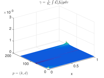
γ𝖪𝗇(x;δy,ϕ):=𝖪𝗇f0(x,v;ϕ)g(x,v;δy)dv,assignsubscript𝛾𝖪𝗇𝑥subscript𝛿𝑦italic-ϕ𝖪𝗇subscript𝑓0𝑥𝑣italic-ϕ𝑔𝑥𝑣subscript𝛿𝑦differential-d𝑣\gamma_{\mathsf{Kn}}(x;\delta_{y},\phi):=\mathsf{Kn}\int f_{0}(x,v;\phi)g(x,v;\delta_{y})\mathrm{d}{v}\,, (23)

then the map 𝒜(σ~a):ϕb(δy,ϕ):𝒜subscript~𝜎𝑎italic-ϕ𝑏subscript𝛿𝑦italic-ϕ\mathcal{A}(\tilde{\sigma}_{a}):~{}\phi\rightarrow b(\delta_{y},\phi) rewrites as

Ωγ𝖪𝗇(x;δy,ϕ)σ~a(x)dx=b(δy,ϕ).subscriptΩsubscript𝛾𝖪𝗇𝑥subscript𝛿𝑦italic-ϕsubscript~𝜎𝑎𝑥differential-d𝑥𝑏subscript𝛿𝑦italic-ϕ\int_{\Omega}\gamma_{\mathsf{Kn}}(x;\delta_{y},\phi)\tilde{\sigma}_{a}(x)\mathrm{d}{x}=b(\delta_{y},\phi)\,. (24)

Now it amounts to invert the First type Fredholm integral to recover σ~asubscript~𝜎𝑎\tilde{\sigma}_{a}.

3.2. Ill-conditioning in the diffusion limit (continuous level)

We study the stability of the inverse problem in terms of the Knudsen number in this subsection. More specifically, consider the linear mapping

γ𝖪𝗇,σ~aL2(dx)=b(δy,ϕ),withγ𝖪𝗇=𝖪𝗇f0gdv,formulae-sequencesubscriptsubscript𝛾𝖪𝗇subscript~𝜎𝑎superscript𝐿2d𝑥𝑏subscript𝛿𝑦italic-ϕwithsubscript𝛾𝖪𝗇𝖪𝗇subscript𝑓0𝑔differential-d𝑣\langle\gamma_{\mathsf{Kn}},\tilde{\sigma}_{a}\rangle_{L^{2}(\mathrm{d}{x})}=b(\delta_{y},\phi)\,,\quad\text{with}\quad\gamma_{\mathsf{Kn}}=\mathsf{Kn}\int f_{0}g\mathrm{d}{v}\,, (25)

where γ𝖪𝗇subscript𝛾𝖪𝗇\gamma_{\mathsf{Kn}} is defined in (23) with f0subscript𝑓0f_{0} and g𝑔g solving (19) and (21), respectively. We aim to understand the influence in recovering σ~asubscript~𝜎𝑎\tilde{\sigma}_{a} if a small purturbation in b(δy,ϕ)𝑏subscript𝛿𝑦italic-ϕb(\delta_{y},\phi) is introduced. In particular, we would like to check such sensitivity’s dependence on the Knudsen number 𝖪𝗇𝖪𝗇\mathsf{Kn}. To see this, we first define a distinguishability coefficient to measure the “condition number” for a given error δ𝛿\delta on data.

Definition 1.

Consider linear mapping in (25), we define the distinguishability coefficient as

κa=supσaΓδσaσ~aL(dx)σ~aL(dx),subscript𝜅𝑎subscriptsupremumsubscript𝜎𝑎subscriptΓ𝛿subscriptnormsubscript𝜎𝑎subscript~𝜎𝑎superscript𝐿d𝑥subscriptnormsubscript~𝜎𝑎subscript𝐿d𝑥\kappa_{a}=\sup_{\sigma_{a}\in\Gamma_{\delta}}\frac{\|\sigma_{a}-\tilde{\sigma}_{a}\|_{L^{\infty}(\mathrm{d}{x})}}{\|\tilde{\sigma}_{a}\|_{L_{\infty}(\mathrm{d}{x})}}\,, (26)

where

Γδ={σa:supϕL(Γ)1,yΩ|γ𝖪𝗇,σaL2(dx)b(δy,ϕ)|δ},subscriptΓ𝛿conditional-setsubscript𝜎𝑎subscriptsupremumfor-allsubscriptnormitalic-ϕsuperscript𝐿subscriptΓ1for-all𝑦Ωsubscriptsubscript𝛾𝖪𝗇subscript𝜎𝑎superscript𝐿2d𝑥𝑏subscript𝛿𝑦italic-ϕ𝛿\Gamma_{\delta}=\{\sigma_{a}:\sup_{\begin{subarray}{c}\forall\|\phi\|_{L^{\infty}(\Gamma_{-})}\leq 1,\\ \forall y\in\partial\Omega\end{subarray}}|\langle\gamma_{\mathsf{Kn}}\,,\sigma_{a}\rangle_{L^{2}(\mathrm{d}{x})}-b(\delta_{y},\phi)|\leq\delta\}\,,

and σ~asubscript~𝜎𝑎\tilde{\sigma}_{a} is the solution to (25).

As written, ΓδsubscriptΓ𝛿\Gamma_{\delta} is the collection of all possible solutions to the map given that the measurement is contaminated by δ𝛿\delta error. Noticed that both γ𝖪𝗇,σaL2(dx)subscriptsubscript𝛾𝖪𝗇subscript𝜎𝑎superscript𝐿2d𝑥\langle\gamma_{\mathsf{Kn}},\sigma_{a}\rangle_{L^{2}(\mathrm{d}{x})} and b(δy,ϕ)𝑏subscript𝛿𝑦italic-ϕb(\delta_{y},\phi) are linearly dependent on ϕitalic-ϕ\phi, we take the sup-norm to normalize in the definition of ΓδsubscriptΓ𝛿\Gamma_{\delta}. Then κasubscript𝜅𝑎\kappa_{a} measures the relative error that could be seen in the recovery — smaller κasubscript𝜅𝑎\kappa_{a} leads to better distinguishability. Recall here that the stability defined in [5] says if the two measurement are distinguished by δ𝛿\delta, i.e., 𝒜σa𝒜σ~aδnorm𝒜subscript𝜎𝑎𝒜subscript~𝜎𝑎𝛿\|\mathcal{A}\sigma_{a}-\mathcal{A}\tilde{\sigma}_{a}\|\leq\delta, then the discrepancy in parameters can be bounded as σaσ~a𝒜1𝒜(σaσ~a)=𝒜1δnormsubscript𝜎𝑎subscript~𝜎𝑎normsuperscript𝒜1norm𝒜subscript𝜎𝑎subscript~𝜎𝑎normsuperscript𝒜1𝛿\|\sigma_{a}-\tilde{\sigma}_{a}\|\leq\|\mathcal{A}^{-1}\|\|\mathcal{A}(\sigma_{a}-\tilde{\sigma}_{a})\|=\|\mathcal{A}^{-1}\|\delta, then κasubscript𝜅𝑎\kappa_{a} defined in (26) is seen as an estimate of 𝒜1normsuperscript𝒜1\|\mathcal{A}^{-1}\|.

We expect to show two things: 1) smaller error tolerance δ𝛿\delta results in better distinguishability; 2) smaller 𝖪𝗇𝖪𝗇\mathsf{Kn} drives the problem into the diffusion limit, leading to worse distinguishability. The following theorem groups the two things together.

Theorem 2.

We study the inverse problem of recovering σ~asubscript~𝜎𝑎\tilde{\sigma}_{a} in  (25). Assume the map from σ~asubscript~𝜎𝑎\tilde{\sigma}_{a} to b𝑏b is injective, given an error tolerance δ𝛿\delta on the measurement, then the distinguishability coefficient grows as δ𝛿\delta grows and 𝖪𝗇𝖪𝗇\mathsf{Kn} shrinks in the sense that there exists a constant C𝐶C such that

κaCδ𝖪𝗇2,when𝖪𝗇1.formulae-sequencesubscript𝜅𝑎𝐶𝛿superscript𝖪𝗇2whenmuch-less-than𝖪𝗇1\kappa_{a}\geq C\frac{\delta}{\mathsf{Kn}^{2}},\quad\text{when}\quad\mathsf{Kn}\ll 1\,. (27)
Proof.

Let c(x)𝑐𝑥c(x) be an arbitrary function such that vanishes in the boundary layer and

|γ𝖪𝗇,cL2(dx)|δ,subscriptsubscript𝛾𝖪𝗇𝑐superscript𝐿2d𝑥𝛿|\langle\gamma_{\mathsf{Kn}},c\rangle_{L^{2}(\mathrm{d}{x})}|\leq\delta\,, (28)

where γ𝖪𝗇subscript𝛾𝖪𝗇\gamma_{\mathsf{Kn}} is defined in (23). Then for such a c(x)𝑐𝑥c(x), one certainly has

σa(x)=σ~a(x)+c(x)Γδ.subscript𝜎𝑎𝑥subscript~𝜎𝑎𝑥𝑐𝑥subscriptΓ𝛿\sigma_{a}(x)=\tilde{\sigma}_{a}(x)+c(x)\in\Gamma_{\delta}\,.

According to Theorem 1, when 𝖪𝗇𝖪𝗇\mathsf{Kn} is small, f0subscript𝑓0f_{0} and g𝑔g approach the diffusion limit. Taking boundary layers into account, we write

f0=fL+fIg=gL+gI,formulae-sequencesubscript𝑓0subscript𝑓𝐿subscript𝑓𝐼𝑔subscript𝑔𝐿subscript𝑔𝐼f_{0}=f_{L}+f_{I}\quad g=g_{L}+g_{I}\,,

where fLsubscript𝑓𝐿f_{L} and gLsubscript𝑔𝐿g_{L} stand for the layers of the two functions, and fIsubscript𝑓𝐼f_{I} and gIsubscript𝑔𝐼g_{I} are the interior solutions. The boundary layers are supported in a thin layer (denoted as ΩLsubscriptΩ𝐿\Omega_{L}) in the vicinity of the boundary ΩΩ\partial\Omega with 𝒪(𝖪𝗇)𝒪𝖪𝗇\mathcal{O}(\mathsf{Kn}) width. The interior fIsubscript𝑓𝐼f_{I} and gIsubscript𝑔𝐼g_{I} supported on ΩI=Ω\ΩLsubscriptΩ𝐼\ΩsubscriptΩ𝐿\Omega_{I}=\Omega\backslash\Omega_{L} are well-approximated by the diffusion limit:

fI=ρf𝖪𝗇vρf+𝒪(𝖪𝗇2),gI=ρg𝖪𝗇vρg+𝒪(𝖪𝗇2),formulae-sequencesubscript𝑓𝐼subscript𝜌𝑓𝖪𝗇𝑣subscript𝜌𝑓𝒪superscript𝖪𝗇2subscript𝑔𝐼subscript𝜌𝑔𝖪𝗇𝑣subscript𝜌𝑔𝒪superscript𝖪𝗇2f_{I}=\rho_{f}-\mathsf{Kn}v\cdot\nabla\rho_{f}+\mathcal{O}(\mathsf{Kn}^{2})\,,\quad g_{I}=\rho_{g}-\mathsf{Kn}v\cdot\nabla\rho_{g}+\mathcal{O}(\mathsf{Kn}^{2})\,,

where ρf,ρgsubscript𝜌𝑓subscript𝜌𝑔\rho_{f},\rho_{g} solve the following equations:

{CΔxρf=σa0ρf,ρf|Ω=ξf(x),casesotherwise𝐶subscriptΔ𝑥subscript𝜌𝑓subscript𝜎𝑎0subscript𝜌𝑓otherwiseevaluated-atsubscript𝜌𝑓Ωsubscript𝜉𝑓𝑥\begin{cases}&C\Delta_{x}\rho_{f}=\sigma_{a0}\rho_{f},\\ &\rho_{f}|_{\partial\Omega}=\xi_{f}(x)\,,\end{cases} (29)

and

{CΔxρg=σa0ρg,ρg|Ω=ξg(x).casesotherwise𝐶subscriptΔ𝑥subscript𝜌𝑔subscript𝜎𝑎0subscript𝜌𝑔otherwiseevaluated-atsubscript𝜌𝑔Ωsubscript𝜉𝑔𝑥\begin{cases}&C\Delta_{x}\rho_{g}=\sigma_{a0}\rho_{g},\\ &\rho_{g}|_{\partial\Omega}=\xi_{g}(x)\,.\end{cases} (30)

Therefore,

γ𝖪𝗇|ΩI=𝖪𝗇fIgIdv=𝖪𝗇ρfρg+𝒪(𝖪𝗇3).evaluated-atsubscript𝛾𝖪𝗇subscriptΩ𝐼𝖪𝗇subscript𝑓𝐼subscript𝑔𝐼differential-d𝑣𝖪𝗇subscript𝜌𝑓subscript𝜌𝑔𝒪superscript𝖪𝗇3\gamma_{\mathsf{Kn}}|_{\Omega_{I}}=\mathsf{Kn}\int f_{I}g_{I}\mathrm{d}{v}=\mathsf{Kn}\rho_{f}\rho_{g}+\mathcal{O}(\mathsf{Kn}^{3})\,.

Plugging it back into (28) and using the fact c(x)=0,xΩLformulae-sequence𝑐𝑥0for-all𝑥subscriptΩ𝐿c(x)=0,\forall x\in\Omega_{L}, we obtain:

γ𝖪𝗇,cL2(dx)subscriptsubscript𝛾𝖪𝗇𝑐superscript𝐿2d𝑥\displaystyle\langle\gamma_{\mathsf{Kn}},c\rangle_{L^{2}(\mathrm{d}{x})} =\displaystyle= ΩIγ𝖪𝗇(x)c(x)dx+ΩLγ𝖪𝗇(x)c(x)dxsubscriptsubscriptΩ𝐼subscript𝛾𝖪𝗇𝑥𝑐𝑥differential-d𝑥subscriptsubscriptΩ𝐿subscript𝛾𝖪𝗇𝑥𝑐𝑥differential-d𝑥\displaystyle\int_{\Omega_{I}}\gamma_{\mathsf{Kn}}(x)c(x)\mathrm{d}x+\int_{\Omega_{L}}\gamma_{\mathsf{Kn}}(x)c(x)\mathrm{d}x (31)
similar-to\displaystyle\sim 𝖪𝗇ΩIρf(x)ρg(x)c(x)dx+𝒪(𝖪𝗇3).𝖪𝗇subscriptsubscriptΩ𝐼subscript𝜌𝑓𝑥subscript𝜌𝑔𝑥𝑐𝑥differential-d𝑥𝒪superscript𝖪𝗇3\displaystyle\mathsf{Kn}\int_{\Omega_{I}}\rho_{f}(x)\rho_{g}(x)c(x)\mathrm{d}{x}+\mathcal{O}(\mathsf{Kn}^{3})\,.

Let G(x,y)𝐺𝑥𝑦G(x,y) be the Green’s function for the operator CΔσa0𝐶Δsubscript𝜎𝑎0C\Delta-\sigma_{a0}, i.e.,

{CΔyGσa0G=δx(y),G|Ω=0.casesotherwise𝐶subscriptΔ𝑦𝐺subscript𝜎𝑎0𝐺subscript𝛿𝑥𝑦otherwiseevaluated-at𝐺Ω0\begin{cases}&C\Delta_{y}G-\sigma_{a0}G=\delta_{x}(y),\\ &G|_{\partial\Omega}=0\,.\end{cases} (32)

Then

ρf(x)=Ωξf(y)Gn(x,y)dμ(y),ρg(x)=Ωξg(y)Gn(x,y)dμ(y),formulae-sequencesubscript𝜌𝑓𝑥subscriptΩsubscript𝜉𝑓𝑦𝐺𝑛𝑥𝑦differential-d𝜇𝑦subscript𝜌𝑔𝑥subscriptΩsubscript𝜉𝑔𝑦𝐺𝑛𝑥𝑦differential-d𝜇𝑦\rho_{f}(x)=\int_{\partial\Omega}\xi_{f}(y)\frac{\partial G}{\partial n}(x,y)\mathrm{d}\mu(y),\quad\rho_{g}(x)=\int_{\partial\Omega}\xi_{g}(y)\frac{\partial G}{\partial n}(x,y)\mathrm{d}\mu(y)\,, (33)

where dμ(y)d𝜇𝑦\mathrm{d}\mu(y) is the surface measure on ΩΩ\partial\Omega. Note that one can find c(x)𝑐𝑥c(x) such that

ΩIρf(x)ρg(x)c(x)dx=𝒪(𝖪𝗇).subscriptsubscriptΩ𝐼subscript𝜌𝑓𝑥subscript𝜌𝑔𝑥𝑐𝑥differential-d𝑥𝒪𝖪𝗇\int_{\Omega_{I}}\rho_{f}(x)\rho_{g}(x)c(x)\mathrm{d}{x}=\mathcal{O}(\mathsf{Kn})\,. (34)

Indeed, using quadrature rule for (33), one has

ρf(x)=jG(x,yj)nξf(yj)wj+𝒪(𝖪𝗇),ρg(x)=jG(x,yj)nξg(yj)wj+𝒪(𝖪𝗇).formulae-sequencesubscript𝜌𝑓𝑥subscript𝑗𝐺𝑥subscript𝑦𝑗𝑛subscript𝜉𝑓subscript𝑦𝑗subscript𝑤𝑗𝒪𝖪𝗇subscript𝜌𝑔𝑥subscript𝑗𝐺𝑥subscript𝑦𝑗𝑛subscript𝜉𝑔subscript𝑦𝑗subscript𝑤𝑗𝒪𝖪𝗇\rho_{f}(x)=\sum_{j}\frac{\partial G(x,y_{j})}{\partial n}\xi_{f}(y_{j})w_{j}+\mathcal{O}(\mathsf{Kn}),\quad\rho_{g}(x)=\sum_{j}\frac{\partial G(x,y_{j})}{\partial n}\xi_{g}(y_{j})w_{j}+\mathcal{O}(\mathsf{Kn})\,.

Thus

ρfρgcdx=i,jξf(yi)ξg(yj)wiwjG(x,yi)nG(x,yj)nc(x)dx+cL(dx)𝒪(𝖪𝗇),subscript𝜌𝑓subscript𝜌𝑔𝑐differential-d𝑥subscript𝑖𝑗subscript𝜉𝑓subscript𝑦𝑖subscript𝜉𝑔subscript𝑦𝑗subscript𝑤𝑖subscript𝑤𝑗𝐺𝑥subscript𝑦𝑖𝑛𝐺𝑥subscript𝑦𝑗𝑛𝑐𝑥differential-d𝑥subscriptnorm𝑐superscript𝐿d𝑥𝒪𝖪𝗇\int\rho_{f}\rho_{g}c\mathrm{d}{x}=\sum_{i,j}\xi_{f}(y_{i})\xi_{g}(y_{j})w_{i}w_{j}\int\frac{\partial G(x,y_{i})}{\partial n}\frac{\partial G(x,y_{j})}{\partial n}c(x)\mathrm{d}{x}+\|c\|_{L^{\infty}(\mathrm{d}{x})}\mathcal{O}(\mathsf{Kn})\,, (35)

then one just need to choose c(x)𝑐𝑥c(x) such that it is perpendicular to the space spanned by {G(x,yi)nG(x,yj)n,i,j}𝐺𝑥subscript𝑦𝑖𝑛𝐺𝑥subscript𝑦𝑗𝑛for-all𝑖𝑗\{\frac{\partial G(x,y_{i})}{\partial n}\frac{\partial G(x,y_{j})}{\partial n},~{}\forall i,j\}. Plugging (34) into (31), we derive that

γ,cL2(dx)cL(dx)𝒪(𝖪𝗇2)+𝒪(𝖪𝗇3).similar-tosubscript𝛾𝑐superscript𝐿2d𝑥subscriptnorm𝑐superscript𝐿d𝑥𝒪superscript𝖪𝗇2𝒪superscript𝖪𝗇3\langle\gamma,c\rangle_{L^{2}(\mathrm{d}{x})}\sim\|c\|_{L^{\infty}(\mathrm{d}{x})}\mathcal{O}(\mathsf{Kn}^{2})+\mathcal{O}(\mathsf{Kn}^{3})\,. (36)

It is seen that to ensure |γ,cL2(dx)|<δsubscript𝛾𝑐superscript𝐿2d𝑥𝛿|\langle\gamma,c\rangle_{L^{2}(\mathrm{d}{x})}|<\delta, one simply needs

cL(dx)𝒪(δ𝖪𝗇2).similar-tosubscriptnorm𝑐superscript𝐿d𝑥𝒪𝛿superscript𝖪𝗇2\|c\|_{L^{\infty}(\mathrm{d}{x})}\sim\mathcal{O}\left(\frac{\delta}{\mathsf{Kn}^{2}}\right)\,.

Considering σ~asubscript~𝜎𝑎\tilde{\sigma}_{a} is of 𝒪(1)𝒪1\mathcal{O}(1), there exists a constant C𝐶C such that κaCδ𝖪𝗇2subscript𝜅𝑎𝐶𝛿superscript𝖪𝗇2\kappa_{a}\geq C\frac{\delta}{\mathsf{Kn}^{2}}, we finish the proof.

Remark 3.

Two immediate take-away information from the theorem:

  • When δ𝛿\delta is small, meaning that the measurement is relatively accurate, then one gets better recovery of the absorption coefficient as expected.

  • When 𝖪𝗇𝖪𝗇\mathsf{Kn} shrinks, the system approaches to the diffusion limit, and the distinguishability coefficient grows dramatically, indicating that the linearized inverse problem is highly ill-conditioned. This phenomena is aligned with the ill-posedness of the Calderón problem.

3.3. Ill-conditioning in the diffusion limit (discrete level)

In this subsection, we revisit the above observation in the discrete setting when solving the inverse problem numerically, in which case the matrix to be inverted becomes highly ill-conditioned as 𝖪𝗇𝖪𝗇\mathsf{Kn} shrinks. Let us sample Nxsubscript𝑁𝑥N_{x} quadrature points in ΩΩ\Omega: xi,i=1,,Nxformulae-sequencesubscript𝑥𝑖𝑖1subscript𝑁𝑥x_{i},i=1,\ldots,N_{x}, and their corresponding weights are denoted by wisubscript𝑤𝑖w_{i}. Suppose the measurements are collected at discrete boundary points {yk}k=1NyΩsuperscriptsubscriptsubscript𝑦𝑘𝑘1subscript𝑁𝑦Ω\{y_{k}\}_{k=1}^{N_{y}}\subset\partial\Omega, and there are ϕd,d=1,2,,Nϕformulae-sequencesubscriptitalic-ϕ𝑑𝑑12subscript𝑁italic-ϕ\phi_{d},d=1,2,\cdots,N_{\phi} different sets of incoming data where supdϕdL(Γ)1subscriptsupremum𝑑subscriptnormsubscriptitalic-ϕ𝑑subscript𝐿superscriptΓ1\sup_{d}\|\phi_{d}\|_{L_{\infty}(\Gamma^{-})}\leq 1. Then the linear system (24) can be rewritten into the form of

d=1,,Nϕ,k=1,,Ny:i=1Nxγ𝖪𝗇(xi;yk,ϕd)σ~a(xi)wi=b(yk,ϕd),\forall d=1,\cdots,N_{\phi},\quad k=1,\cdots,N_{y}:\quad\sum_{i=1}^{N_{x}}\gamma_{\mathsf{Kn}}(x_{i};y_{k},\phi_{d})\tilde{\sigma}_{a}(x_{i})w_{i}=b(y_{k},\phi_{d})\,, (37)

with

γ𝖪𝗇(xi;yk,ϕd)=𝖪𝗇f0(xi,v;ϕd)g(xi,v;δyk)dv,subscript𝛾𝖪𝗇subscript𝑥𝑖subscript𝑦𝑘subscriptitalic-ϕ𝑑𝖪𝗇subscript𝑓0subscript𝑥𝑖𝑣subscriptitalic-ϕ𝑑𝑔subscript𝑥𝑖𝑣subscript𝛿subscript𝑦𝑘differential-d𝑣\gamma_{\mathsf{Kn}}(x_{i};y_{k},\phi_{d})=\mathsf{Kn}\int f_{0}(x_{i},v;\phi_{d})g(x_{i},v;\delta_{y_{k}})\mathrm{d}{v}\,,

and f0subscript𝑓0f_{0} and g𝑔g solve (19) and (21) respectively with ϕdsubscriptitalic-ϕ𝑑\phi_{d} and δyksubscript𝛿subscript𝑦𝑘\delta_{y_{k}} as boundary condition, here δyksubscript𝛿subscript𝑦𝑘\delta_{y_{k}} is hat function centered at x=yk𝑥subscript𝑦𝑘x=y_{k}. For simplicity we use index p𝑝p to denote sub-index k𝑘k and d𝑑d. Then the linear system (37) can be further written into a compact form:

𝖠σ~𝐚=𝐛,𝖠subscript~𝜎𝐚𝐛\mathsf{A}\mathbf{\tilde{\sigma}_{a}}=\mathbf{b}\,, (38)

where 𝖠Np×Nx𝖠superscriptsubscript𝑁𝑝subscript𝑁𝑥\mathsf{A}\in\mathbb{R}^{N_{p}\times N_{x}} with entries 𝖠pi=γ𝖪𝗇(xi;yk,ϕd)wisubscript𝖠𝑝𝑖subscript𝛾𝖪𝗇subscript𝑥𝑖subscript𝑦𝑘subscriptitalic-ϕ𝑑subscript𝑤𝑖\mathsf{A}_{pi}=\gamma_{\mathsf{Kn}}(x_{i};y_{k},\phi_{d})w_{i} such that (k,d)=p𝑘𝑑𝑝(k,d)=p. σ~𝐚Nxsubscript~𝜎𝐚superscriptsubscript𝑁𝑥\mathbf{\tilde{\sigma}_{a}}\in\mathbb{R}^{N_{x}} is the discretization of σ~asubscript~𝜎𝑎\tilde{\sigma}_{a} on Nxsubscript𝑁𝑥N_{x} quadrature nodes, and data 𝐛Np𝐛superscriptsubscript𝑁𝑝\mathbf{b}\in\mathbb{R}^{N_{p}}. Here Np=Ny×Nϕsubscript𝑁𝑝subscript𝑁𝑦subscript𝑁italic-ϕN_{p}=N_{y}\times N_{\phi} denotes the total number of data points we have, and it is a product of Nϕsubscript𝑁italic-ϕN_{\phi}, the number of inflow data and Nysubscript𝑁𝑦N_{y}, the number of measurement positions. We show below that as 𝖪𝗇0𝖪𝗇0\mathsf{Kn}\to 0 the matrix 𝖠𝖠\mathsf{A} becomes more and more singular, making the inversion impossible.

Theorem 3.

Assume that 𝖠𝖠\mathsf{A} is nonsingular. When 𝖪𝗇𝖪𝗇\mathsf{Kn} is small, the condition number of matrix 𝖠T𝖠superscript𝖠𝑇𝖠\mathsf{A}^{T}\mathsf{A} scales as

κ(𝖠T𝖠)C1𝖪𝗇,for some constantC.𝜅superscript𝖠𝑇𝖠𝐶1𝖪𝗇for some constant𝐶\kappa(\mathsf{A}^{T}\mathsf{A})\geq C\frac{1}{\mathsf{Kn}}\,,\quad\text{for some constant}\quad C\,. (39)

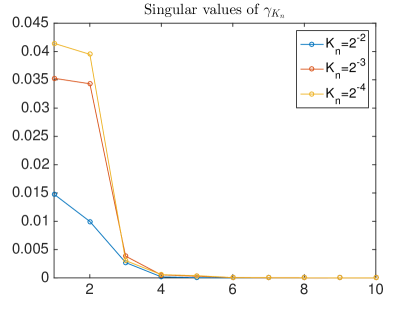
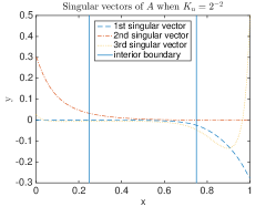
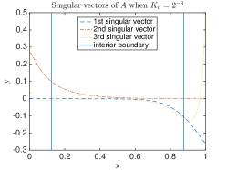
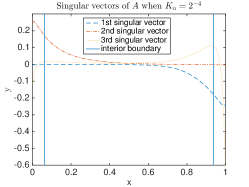
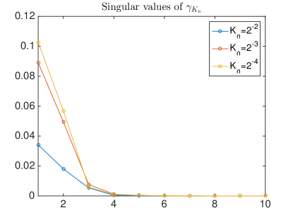
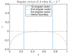
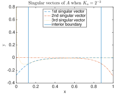
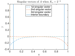
Moreover, in 1D, 𝖠𝖠\mathsf{A} is approximately low rank, in the sense that it only has no more than 3 singular values of size 𝒪(𝖪𝗇)𝒪𝖪𝗇\mathcal{O}(\mathsf{Kn}), and all the rest are of size 𝒪(𝖪𝗇3/2)𝒪superscript𝖪𝗇32\mathcal{O}(\mathsf{Kn}^{3/2}).

Proof.

We first the prove the theorem in any dimension and refine the result in 1D. According to the diffusion theory, in the zero limit of 𝖪𝗇𝖪𝗇\mathsf{Kn}, 𝖠𝖠\mathsf{A} can be decomposed into two parts:

𝖠=𝖪𝗇(𝖠L𝖠I),𝖠𝖪𝗇matrixsubscript𝖠𝐿subscript𝖠𝐼\mathsf{A}=\mathsf{Kn}\begin{pmatrix}\mathsf{A}_{L}&\mathsf{A}_{I}\end{pmatrix}\,, (40)

where 𝖠LNp×NL,(NLNx)subscript𝖠𝐿superscriptsubscript𝑁𝑝subscript𝑁𝐿much-less-thansubscript𝑁𝐿subscript𝑁𝑥\mathsf{A}_{L}\in\mathbb{R}^{N_{p}\times N_{L}},~{}(N_{L}\ll N_{x}) are the sampled points in the layer, and 𝖠INp×(NxNL)subscript𝖠𝐼superscriptsubscript𝑁𝑝subscript𝑁𝑥subscript𝑁𝐿\mathsf{A}_{I}\in\mathbb{R}^{N_{p}\times(N_{x}-N_{L})} represents the sampled points in the interior. To analyze the rank of the matrix, we rewrite 𝖠T𝖠superscript𝖠𝑇𝖠\mathsf{A}^{T}\mathsf{A} as

𝖠T𝖠=𝖪𝗇2(𝖠LT𝖠L𝖠LT𝖠I𝖠IT𝖠L𝖠IT𝖠I).superscript𝖠𝑇𝖠superscript𝖪𝗇2matrixsuperscriptsubscript𝖠𝐿𝑇subscript𝖠𝐿subscriptsuperscript𝖠𝑇𝐿subscript𝖠𝐼superscriptsubscript𝖠𝐼𝑇subscript𝖠𝐿subscriptsuperscript𝖠𝑇𝐼subscript𝖠𝐼\mathsf{A}^{T}\mathsf{A}=\mathsf{Kn}^{2}\begin{pmatrix}\mathsf{A}_{L}^{T}\mathsf{A}_{L}&\mathsf{A}^{T}_{L}\mathsf{A}_{I}\\ \mathsf{A}_{I}^{T}\mathsf{A}_{L}&\mathsf{A}^{T}_{I}\mathsf{A}_{I}\\ \end{pmatrix}\,.

When 𝖪𝗇𝖪𝗇\mathsf{Kn} is small, 𝖠I=𝖠I0+𝒪(𝖪𝗇)subscript𝖠𝐼subscriptsuperscript𝖠0𝐼𝒪𝖪𝗇\mathsf{A}_{I}=\mathsf{A}^{0}_{I}+\mathcal{O}(\mathsf{Kn}), where each row in 𝖠I0superscriptsubscript𝖠𝐼0\mathsf{A}_{I}^{0} are:

ρf(xi;ϕd)ρg(xi;yk)wi,i=1,2,Nx.formulae-sequencesubscript𝜌𝑓subscript𝑥𝑖subscriptitalic-ϕ𝑑subscript𝜌𝑔subscript𝑥𝑖subscript𝑦𝑘subscript𝑤𝑖𝑖12subscript𝑁𝑥\rho_{f}(x_{i};\phi_{d})\rho_{g}(x_{i};y_{k})w_{i},\qquad i=1,2,\cdots N_{x}\,. (41)

Therefore, 𝖠T𝖠=𝖪𝗇2𝖯+𝒪(𝖪𝗇3)superscript𝖠𝑇𝖠superscript𝖪𝗇2𝖯𝒪superscript𝖪𝗇3\mathsf{A}^{T}\mathsf{A}=\mathsf{Kn}^{2}\mathsf{P}+\mathcal{O}(\mathsf{Kn}^{3}), where

𝖯=(𝖠LT𝖠L𝖠LT𝖠I𝖠IT𝖠L𝖠I0T𝖠I0)=(000𝖠I0T𝖠I0)+(𝖠LT𝖠L𝖠LT𝖠I𝖠IT𝖠L0).𝖯matrixsuperscriptsubscript𝖠𝐿𝑇subscript𝖠𝐿subscriptsuperscript𝖠𝑇𝐿subscript𝖠𝐼superscriptsubscript𝖠𝐼𝑇subscript𝖠𝐿subscriptsuperscript𝖠0𝑇𝐼subscriptsuperscript𝖠0𝐼matrix000subscriptsuperscript𝖠0𝑇𝐼superscriptsubscript𝖠𝐼0matrixsuperscriptsubscript𝖠𝐿𝑇subscript𝖠𝐿subscriptsuperscript𝖠𝑇𝐿subscript𝖠𝐼superscriptsubscript𝖠𝐼𝑇subscript𝖠𝐿0\mathsf{P}=\begin{pmatrix}\mathsf{A}_{L}^{T}\mathsf{A}_{L}&\mathsf{A}^{T}_{L}\mathsf{A}_{I}\\ \mathsf{A}_{I}^{T}\mathsf{A}_{L}&\mathsf{A}^{0T}_{I}\mathsf{A}^{0}_{I}\end{pmatrix}=\begin{pmatrix}0&0\\ 0&\mathsf{A}^{0T}_{I}\mathsf{A}_{I}^{0}\end{pmatrix}+\begin{pmatrix}\mathsf{A}_{L}^{T}\mathsf{A}_{L}&\mathsf{A}^{T}_{L}\mathsf{A}_{I}\\ \mathsf{A}_{I}^{T}\mathsf{A}_{L}&0\\ \end{pmatrix}\,.

Since 𝖠I0T𝖠I0superscriptsubscript𝖠𝐼0𝑇superscriptsubscript𝖠𝐼0\mathsf{A}_{I}^{0T}\mathsf{A}_{I}^{0} is symmetric, it is diagonizable. Denote:

𝖠I0T𝖠I0=𝖰𝖣𝖰1,superscriptsubscript𝖠𝐼0𝑇superscriptsubscript𝖠𝐼0superscript𝖰𝖣𝖰1\mathsf{A}_{I}^{0T}\mathsf{A}_{I}^{0}=\mathsf{Q}\mathsf{D}\mathsf{Q}^{-1}\,, (42)

with 𝖰(NxNL)×(NxNL)𝖰superscriptsubscript𝑁𝑥subscript𝑁𝐿subscript𝑁𝑥subscript𝑁𝐿\mathsf{Q}\in\mathbb{R}^{(N_{x}-N_{L})\times(N_{x}-N_{L})} the collection of eigenvectors and 𝖣𝖣\mathsf{D} the diagonal matrix of eigenvalues. Then we multiply both sides by matrix 𝖷𝖷\mathsf{X} and 𝖷1superscript𝖷1\mathsf{X}^{-1} defined as below

𝖷=(𝕀00𝖰),𝖷1=(𝕀00𝖰1),formulae-sequence𝖷matrix𝕀00𝖰superscript𝖷1matrix𝕀00superscript𝖰1\mathsf{X}=\begin{pmatrix}\mathbb{I}&0\\ 0&\mathsf{Q}\\ \end{pmatrix},\quad\mathsf{X}^{-1}=\begin{pmatrix}\mathbb{I}&0\\ 0&\mathsf{Q}^{-1}\\ \end{pmatrix}\,,

we derive that

𝖷1𝖠T𝖠𝖷=𝖪𝗇2(000𝖣)+𝖪𝗇2(𝖠LT𝖠L𝖠LT𝖠I𝖰𝖰1𝖠IT𝖠L0)+𝒪(𝖪𝗇3).superscript𝖷1superscript𝖠𝑇𝖠𝖷superscript𝖪𝗇2matrix000𝖣superscript𝖪𝗇2matrixsuperscriptsubscript𝖠𝐿𝑇subscript𝖠𝐿subscriptsuperscript𝖠𝑇𝐿subscript𝖠𝐼𝖰superscript𝖰1superscriptsubscript𝖠𝐼𝑇subscript𝖠𝐿0𝒪superscript𝖪𝗇3\mathsf{X}^{-1}\mathsf{A}^{T}\mathsf{A}\mathsf{X}=\mathsf{Kn}^{2}\begin{pmatrix}0&0\\ 0&\mathsf{D}\\ \end{pmatrix}+\mathsf{Kn}^{2}\begin{pmatrix}\mathsf{A}_{L}^{T}\mathsf{A}_{L}&\mathsf{A}^{T}_{L}\mathsf{A}_{I}\mathsf{Q}\\ \mathsf{Q}^{-1}\mathsf{A}_{I}^{T}\mathsf{A}_{L}&0\\ \end{pmatrix}\,+\mathcal{O}(\mathsf{Kn}^{3})\,.

Note that the number of elements in ALsubscript𝐴𝐿A_{L} is of order 𝒪(𝖪𝗇)𝒪𝖪𝗇\mathcal{O}(\mathsf{Kn}) due to the fact that the layer length is order of 𝒪(𝖪𝗇)𝒪𝖪𝗇\mathcal{O}(\mathsf{Kn}), and its elements are order 𝒪(1)𝒪1\mathcal{O}(1) thanks to the maximal principle: the integrand function |fLgL|ϕL(Γ)δykL(dx)=𝒪(1)subscript𝑓𝐿subscript𝑔𝐿subscriptnormitalic-ϕsuperscript𝐿subscriptΓsubscriptnormsubscript𝛿subscript𝑦𝑘superscript𝐿d𝑥𝒪1|f_{L}g_{L}|\leq\|\phi\|_{L^{\infty}(\Gamma_{-})}\|\delta_{y_{k}}\|_{L^{\infty}(\mathrm{d}{x})}=\mathcal{O}(1). Therefore, we could rewrite the equation above:

𝖷1𝖠T𝖠𝖷=𝖪𝗇2(000𝖣)+𝒪(𝖪𝗇3):=𝖪𝗇2𝖣1+𝒪(𝖪𝗇3).superscript𝖷1superscript𝖠𝑇𝖠𝖷superscript𝖪𝗇2matrix000𝖣𝒪superscript𝖪𝗇3assignsuperscript𝖪𝗇2subscript𝖣1𝒪superscript𝖪𝗇3\mathsf{X}^{-1}\mathsf{A}^{T}\mathsf{A}\mathsf{X}=\mathsf{Kn}^{2}\begin{pmatrix}0&0\\ 0&\mathsf{D}\\ \end{pmatrix}+\mathcal{O}(\mathsf{Kn}^{3}):=\mathsf{Kn}^{2}\mathsf{D}_{1}+\mathcal{O}(\mathsf{Kn}^{3})\,.

By Gershgorin circle theorem, all eigenvalues lie in Gershgorin disc, meaning that |λ(𝖠T𝖠)λ(𝖪𝗇2𝖣1)|<𝒪(𝖪𝗇3)𝜆superscript𝖠𝑇𝖠𝜆superscript𝖪𝗇2subscript𝖣1𝒪superscript𝖪𝗇3|\lambda(\mathsf{A}^{T}\mathsf{A})-\lambda(\mathsf{Kn}^{2}\mathsf{D}_{1})|<\mathcal{O}(\mathsf{Kn}^{3}). Since the eigenvalues in 𝖣1subscript𝖣1\mathsf{D}_{1} can be 𝒪(1)𝒪1\mathcal{O}(1) or 0, the largest eigenvalue in 𝖠T𝖠superscript𝖠𝑇𝖠\mathsf{A}^{T}\mathsf{A} is 𝒪(𝖪𝗇2)𝒪superscript𝖪𝗇2\mathcal{O}(\mathsf{Kn}^{2}) and the smallest is 𝒪(𝖪𝗇3)𝒪superscript𝖪𝗇3\mathcal{O}(\mathsf{Kn}^{3}), the condition number of 𝖠T𝖠superscript𝖠𝑇𝖠\mathsf{A}^{T}\mathsf{A} is larger than 𝒪(1𝖪𝗇)𝒪1𝖪𝗇\mathcal{O}\left(\frac{1}{\mathsf{Kn}}\right).

Moreover, in 1D, we show in the appendix that 𝖣𝖣\mathsf{D} is indeed a low rank matrix itself with rank not exceeding 3. Therefore, there are at most 3 nonzero eigenvalues in 𝖣𝖣\mathsf{D} and all the rest are zeros. Putting this information back to 𝖠𝖠\mathsf{A}, the result directly follows.

Remark 4.

We emphasize the difference between Theorem 2 and Theorem 3. Theorem 2 is the study of κasubscript𝜅𝑎\kappa_{a}, which represents 𝒜1normsuperscript𝒜1\|\mathcal{A}^{-1}\|: it tells that suppose the measurement is different, how different could σasubscript𝜎𝑎\sigma_{a} be. However, numerically it is the condition number of 𝖠𝖠\mathsf{A} that is playing the role. If 𝖠𝖠\mathsf{A} is low rank, for example, rank k𝑘k out of an n𝑛n dimensional space, then there are infinite many σasubscript𝜎𝑎\sigma_{a} that could lead to the same measurement and the space they span is nk𝑛𝑘n-k dimensional.

Similar to the analysis on the continuous level, we immediately conclude that the ill-conditioned matrix 𝖠𝖠\mathsf{A} in 𝖪𝗇0𝖪𝗇0\mathsf{Kn}\to 0 limit leads to the fact that σasubscript𝜎𝑎\sigma_{a} is hard to be recovered accurately, which is consistent with the ill-posedness of the Calderón problem. More precisely, we have the following estimate theorem.

Theorem 4.

Define the distinguishability coefficient in the discrete setting as

κa=supσaΓδσaσ~aσ~a,subscript𝜅𝑎subscriptsupremumsubscript𝜎𝑎subscriptΓ𝛿normsubscript𝜎𝑎subscript~𝜎𝑎normsubscript~𝜎𝑎\kappa_{a}=\sup_{\sigma_{a}\in\Gamma_{\delta}}\frac{\|\sigma_{a}-\tilde{\sigma}_{a}\|}{\|\tilde{\sigma}_{a}\|}\,,

where \|\cdot\| denote vector l2superscript𝑙2l^{2}-norm and 𝖠σ~a=b𝖠subscript~𝜎𝑎𝑏\mathsf{A}\tilde{\sigma}_{a}=b, and Γδ={σa:𝖠σabδ}subscriptΓ𝛿conditional-setsubscript𝜎𝑎norm𝖠subscript𝜎𝑎𝑏𝛿\Gamma_{\delta}=\{\sigma_{a}:\|\mathsf{A}\sigma_{a}-b\|\leq\delta\}. Assume that 𝖠𝖠\mathsf{A} is nonsingular, then there exists a constant C𝐶C such that

κaCδ𝖪𝗇2+𝖪𝗇Δx.subscript𝜅𝑎𝐶𝛿superscript𝖪𝗇2𝖪𝗇Δ𝑥\kappa_{a}\geq C\frac{\delta}{\mathsf{Kn}^{2}+\mathsf{Kn}\Delta x}\,. (43)
Proof.

We again decompose 𝖠𝖠\mathsf{A} as in (40). Note that for each row of 𝖠Isubscript𝖠𝐼\mathsf{A}_{I}, we have

(𝖠I)i=f0(xi,v;ϕd)g(xi,v;yk)dvwi=ρf(xi;ϕd)ρg(xi;yk)wi+𝒪(𝖪𝗇2),subscriptsubscript𝖠𝐼𝑖subscript𝑓0subscript𝑥𝑖𝑣subscriptitalic-ϕ𝑑𝑔subscript𝑥𝑖𝑣subscript𝑦𝑘differential-d𝑣subscript𝑤𝑖subscript𝜌𝑓subscript𝑥𝑖subscriptitalic-ϕ𝑑subscript𝜌𝑔subscript𝑥𝑖subscript𝑦𝑘subscript𝑤𝑖𝒪superscript𝖪𝗇2(\mathsf{A}_{I})_{i}=\int f_{0}(x_{i},v;\phi_{d})g(x_{i},v;y_{k})\mathrm{d}{v}w_{i}=\rho_{f}(x_{i};\phi_{d})\rho_{g}(x_{i};y_{k})w_{i}+\mathcal{O}(\mathsf{Kn}^{2})\,,

where

ρf(xi;ϕd)=jG(xi,yj)nξϕd(yj)wj=G(xi,y)nξϕd(y)dy+𝒪(Δy),subscript𝜌𝑓subscript𝑥𝑖subscriptitalic-ϕ𝑑subscript𝑗𝐺subscript𝑥𝑖subscript𝑦𝑗𝑛subscript𝜉subscriptitalic-ϕ𝑑subscript𝑦𝑗subscript𝑤𝑗𝐺subscript𝑥𝑖𝑦𝑛subscript𝜉subscriptitalic-ϕ𝑑𝑦differential-d𝑦𝒪Δ𝑦\displaystyle\rho_{f}(x_{i};\phi_{d})=\sum_{j}\frac{\partial G(x_{i},y_{j})}{\partial n}\xi_{\phi_{d}}(y_{j})w_{j}=\int\frac{\partial G(x_{i},y)}{\partial n}\xi_{\phi_{d}}(y)\mathrm{d}{y}+\mathcal{O}(\Delta y)\,,
ρg(xi;yk)=jG(xi,yj)nξδyk(yj)wj=G(xi,y)nξδyk(y)dy+𝒪(Δy).subscript𝜌𝑔subscript𝑥𝑖subscript𝑦𝑘subscript𝑗𝐺subscript𝑥𝑖subscript𝑦𝑗𝑛subscript𝜉subscript𝛿subscript𝑦𝑘subscript𝑦𝑗subscript𝑤𝑗𝐺subscript𝑥𝑖𝑦𝑛subscript𝜉subscript𝛿subscript𝑦𝑘𝑦differential-d𝑦𝒪Δ𝑦\displaystyle\rho_{g}(x_{i};y_{k})=\sum_{j}\frac{\partial G(x_{i},y_{j})}{\partial n}\xi_{\delta_{y_{k}}}(y_{j})w_{j}=\int\frac{\partial G(x_{i},y)}{\partial n}\xi_{\delta_{y_{k}}}(y)\mathrm{d}{y}+\mathcal{O}(\Delta y)\,.

Here G(x,y)𝐺𝑥𝑦G(x,y) is the Green’s function defined in (32) and Δy=maxiΔyiΔ𝑦subscript𝑖Δsubscript𝑦𝑖\Delta y=\max_{i}\Delta y_{i}. Denote 𝐜=σaσ~a𝐜subscript𝜎𝑎subscript~𝜎𝑎\mathbf{c}=\mathbf{\sigma}_{a}-\mathbf{\tilde{\sigma}}_{a}, then

𝖠𝐜δ.norm𝖠𝐜𝛿\|\mathsf{A}\mathbf{c}\|\leq\delta\,. (44)

Since

𝖠𝐜=𝖪𝗇𝖠L𝐜L+𝖪𝗇𝖠I𝐜I=𝒪(𝖪𝗇2)𝐜L+𝖪𝗇𝖠I𝐜I,𝖠𝐜subscript𝖪𝗇𝖠𝐿subscript𝐜𝐿subscript𝖪𝗇𝖠𝐼subscript𝐜𝐼𝒪superscript𝖪𝗇2subscript𝐜𝐿subscript𝖪𝗇𝖠𝐼subscript𝐜𝐼\mathsf{A}\mathbf{c}=\mathsf{Kn}\mathsf{A}_{L}\mathbf{c}_{L}+\mathsf{Kn}\mathsf{A}_{I}\mathbf{c}_{I}=\mathcal{O}(\mathsf{Kn}^{2})\mathbf{c}_{L}+\mathcal{\mathsf{Kn}}\mathsf{A}_{I}\mathbf{c}_{I}\,,

and from (3.3), one can always choose 𝐜Isubscript𝐜𝐼\mathbf{c}_{I} as long as Nϕ×Ny<Nxsubscript𝑁italic-ϕsubscript𝑁𝑦subscript𝑁𝑥N_{\phi}\times N_{y}<N_{x} (just pick cIsubscript𝑐𝐼c_{I} from (35) ) such that

i=1Nxρf(xi;ϕd)ρg(xi;yk)𝐜I(xi)wi=𝒪(Δy),ϕd,yk,superscriptsubscript𝑖1subscript𝑁𝑥subscript𝜌𝑓subscript𝑥𝑖subscriptitalic-ϕ𝑑subscript𝜌𝑔subscript𝑥𝑖subscript𝑦𝑘subscript𝐜𝐼subscript𝑥𝑖subscript𝑤𝑖𝒪Δ𝑦for-allsubscriptitalic-ϕ𝑑subscript𝑦𝑘\sum_{i=1}^{N_{x}}\rho_{f}(x_{i};\phi_{d})\rho_{g}(x_{i};y_{k})\mathbf{c}_{I}(x_{i})w_{i}=\mathcal{O}(\Delta y),\quad\forall\phi_{d},~{}y_{k}\,,

we have

𝖠𝐜=𝒪(𝖪𝗇2)𝐜L+𝒪(𝖪𝗇Δy)𝐜I.𝖠𝐜𝒪superscript𝖪𝗇2subscript𝐜𝐿𝒪𝖪𝗇Δ𝑦subscript𝐜𝐼\mathsf{A}\mathbf{c}=\mathcal{O}(\mathsf{Kn}^{2})\mathbf{c}_{L}+\mathcal{O}(\mathsf{Kn}\Delta y)\mathbf{c}_{I}\,.

Therefore, the requirement (44) implies (43). ∎

4. Recover Scattering Coefficient σssubscript𝜎𝑠\sigma_{s}

In this section we discuss how to recover the scattering coefficient given σasubscript𝜎𝑎\sigma_{a}. In subsection 4.1 we set up the inverse problem, and the following two subsections are devoted to the non-injectivity in 1D and ill-conditioning in multi-dimension in the zero limit of the Knudsen number.

4.1. Inverse problem set-up

We recall the equation again:

{vxf=1𝖪𝗇σsf𝖪𝗇σaf,(x,v)Ω×𝕊,f|Γ=ϕ.cases𝑣subscript𝑥𝑓1𝖪𝗇subscript𝜎𝑠𝑓𝖪𝗇subscript𝜎𝑎𝑓𝑥𝑣Ω𝕊evaluated-at𝑓subscriptΓitalic-ϕotherwise\begin{cases}v\cdot\nabla_{x}f=\frac{1}{\mathsf{Kn}}\sigma_{s}\mathcal{L}f-\mathsf{Kn}\sigma_{a}f\,,\quad&(x,v)\in\Omega\times\mathbb{S}\,,\\ f|_{\Gamma_{-}}=\phi\,.&\\ \end{cases} (45)

Here σasubscript𝜎𝑎\sigma_{a} as known, and we make a guess for σssubscript𝜎𝑠\sigma_{s}, and linearize the equation around σs0subscript𝜎𝑠0\sigma_{s0}, assuming the deviation |σ~s|:=|σsσs0|assignsubscript~𝜎𝑠subscript𝜎𝑠subscript𝜎𝑠0|\tilde{\sigma}_{s}|:=|\sigma_{s}-\sigma_{s0}| is much smaller than σssubscript𝜎𝑠\sigma_{s}. The background solution f0subscript𝑓0f_{0} solves

{vxf0=1𝖪𝗇σs0f0𝖪𝗇σaf0,f0|Γ=ϕ.cases𝑣subscript𝑥subscript𝑓01𝖪𝗇subscript𝜎𝑠0subscript𝑓0𝖪𝗇subscript𝜎𝑎subscript𝑓0otherwiseevaluated-atsubscript𝑓0subscriptΓitalic-ϕotherwise\begin{cases}v\cdot\nabla_{x}f_{0}=\frac{1}{\mathsf{Kn}}\sigma_{s0}\mathcal{L}f_{0}-\mathsf{Kn}\sigma_{a}f_{0}\,,\\ f_{0}|_{\Gamma_{-}}=\phi\,.\end{cases} (46)

As done in the last section, we drop the higher order terms, and the fluctuation f~:=ff0assign~𝑓𝑓subscript𝑓0\tilde{f}:=f-f_{0} satisfies the following equation:

{vxf~=1𝖪𝗇σs0f~+1𝖪𝗇σ~sf0𝖪𝗇σaf~,f~|Γ=0.cases𝑣subscript𝑥~𝑓1𝖪𝗇subscript𝜎𝑠0~𝑓1𝖪𝗇subscript~𝜎𝑠subscript𝑓0𝖪𝗇subscript𝜎𝑎~𝑓otherwiseevaluated-at~𝑓subscriptΓ0otherwise\begin{cases}v\cdot\nabla_{x}\tilde{f}=\frac{1}{\mathsf{Kn}}\sigma_{s0}\mathcal{L}\tilde{f}+\frac{1}{\mathsf{Kn}}\tilde{\sigma}_{s}\mathcal{L}f_{0}-\mathsf{Kn}\sigma_{a}\tilde{f}\,,\\ \tilde{f}|_{\Gamma_{-}}=0\,.\\ \end{cases} (47)

To recover σ~ssubscript~𝜎𝑠\tilde{\sigma}_{s}, we look for the linear mapping from the incoming information ϕitalic-ϕ\phi to some computable quantity b(δy,ϕ)𝑏subscript𝛿𝑦italic-ϕb(\delta_{y},\phi) (to be determined below), i.e.,

ϕb(δy,ϕ).italic-ϕ𝑏subscript𝛿𝑦italic-ϕ\phi\rightarrow b(\delta_{y},\phi)\,.

To this end, we consider an auxiliary function g(x,v)𝑔𝑥𝑣g(x,v) that satisfies the adjoint problem:

{vxg=1𝖪𝗇σs0g𝖪𝗇σag,g|Γ+=δy(x).cases𝑣subscript𝑥𝑔1𝖪𝗇subscript𝜎𝑠0𝑔𝖪𝗇subscript𝜎𝑎𝑔otherwiseevaluated-at𝑔subscriptΓsubscript𝛿𝑦𝑥otherwise\begin{cases}-v\cdot\nabla_{x}g=\frac{1}{\mathsf{Kn}}\sigma_{s0}\mathcal{L}g-\mathsf{Kn}\sigma_{a}g\,,\\ g|_{\Gamma_{+}}=\delta_{y}(x)\,.\\ \end{cases}\, (48)

Multiply Equation (47) with g𝑔g and (48) with f~~𝑓\tilde{f} and compare these two equations, with the Green’s identity, one gets:

Γ+(y)vn(y)f~(y,v;ϕ)dv=1𝖪𝗇σ~s(x)g(x,v;δy)f0(x,v;ϕ)dvdx.subscriptsubscriptΓ𝑦𝑣𝑛𝑦~𝑓𝑦𝑣italic-ϕdifferential-d𝑣1𝖪𝗇subscript~𝜎𝑠𝑥𝑔𝑥𝑣subscript𝛿𝑦subscript𝑓0𝑥𝑣italic-ϕdifferential-d𝑣differential-d𝑥\int_{\Gamma_{+}(y)}v\cdot n(y)\tilde{f}(y,v;\phi)\mathrm{d}v=\frac{1}{\mathsf{Kn}}\int\tilde{\sigma}_{s}(x)\int g(x,v;\delta_{y})\mathcal{L}f_{0}(x,v;\phi)\mathrm{d}v\mathrm{d}x\,. (49)

Then we define:

γ𝖪𝗇(x;δy,ϕ):=1𝖪𝗇g(x,v;δy)f0(x,v;ϕ)dv,assignsubscript𝛾𝖪𝗇𝑥subscript𝛿𝑦italic-ϕ1𝖪𝗇𝑔𝑥𝑣subscript𝛿𝑦subscript𝑓0𝑥𝑣italic-ϕdifferential-d𝑣\gamma_{\mathsf{Kn}}(x;\delta_{y},\phi):=\frac{1}{\mathsf{Kn}}\int g(x,v;\delta_{y})\mathcal{L}f_{0}(x,v;\phi)\mathrm{d}{v}\,, (50)

then (49) becomes:

γ𝖪𝗇(x;δy,ϕ)σ~s(x)dx=b(δy,ϕ),subscript𝛾𝖪𝗇𝑥subscript𝛿𝑦italic-ϕsubscript~𝜎𝑠𝑥differential-d𝑥𝑏subscript𝛿𝑦italic-ϕ\int\gamma_{\mathsf{Kn}}(x;\delta_{y},\phi)\tilde{\sigma}_{s}(x)\mathrm{d}{x}=b(\delta_{y},\phi)\,, (51)

where

b(δy,ϕ)=(ff0)(y;ϕ),𝑏subscript𝛿𝑦italic-ϕ𝑓subscript𝑓0𝑦italic-ϕb(\delta_{y},\phi)=\mathcal{M}(f-f_{0})(y;\phi)\,,

which is again the difference between the measured data and computed data, given by the boundary condition ϕitalic-ϕ\phi, evaluated at y𝑦y. The inverse problem then is equivalent to the Fredholm first type problem: for all y𝑦y and ϕitalic-ϕ\phi, we prepare γ(x;δy,ϕ)𝛾𝑥subscript𝛿𝑦italic-ϕ\gamma(x;\delta_{y},\phi) and b(δy,ϕ)𝑏subscript𝛿𝑦italic-ϕb(\delta_{y},\phi), and use them to invert for σssubscript𝜎𝑠\sigma_{s}. For the ease of notation we write b(y,ϕ)𝑏𝑦italic-ϕb(y,\phi) as b(δy,ϕ)𝑏subscript𝛿𝑦italic-ϕb(\delta_{y},\phi) with δysubscript𝛿𝑦\delta_{y} representing the boundary condition for g𝑔g.

4.2. Non-injectivity in 1D

Similar to the case of recovering σasubscript𝜎𝑎\sigma_{a}, recovering σssubscript𝜎𝑠\sigma_{s} becomes harder as 𝖪𝗇𝖪𝗇\mathsf{Kn} shrinks to zero. In 1D, formulae can be made explicitly.

We first restrict our attention to the critical case by setting σa0subscript𝜎𝑎0\sigma_{a}\equiv 0. When there is no absorption, the only interaction between particles is scattering, and thus mass is preserved. We show below that in this case, the problem is non-injective in the sense that γ𝛾\gamma cannot provide enough variations to distinguish σssubscript𝜎𝑠\sigma_{s} at different x𝑥x, and that different σssubscript𝜎𝑠\sigma_{s} could lead to the same measurement provided the same data.

Proposition 1.

Given arbitrary ϕdsubscriptitalic-ϕ𝑑\phi_{d} and δysubscript𝛿𝑦\delta_{y}, let f0subscript𝑓0f_{0} solve (46) and g𝑔g solve (48). Let γ𝖪𝗇subscript𝛾𝖪𝗇\gamma_{\mathsf{Kn}} be defined in (50). Then in 1D, if σa0subscript𝜎𝑎0\sigma_{a}\equiv 0, γ𝖪𝗇subscript𝛾𝖪𝗇\gamma_{\mathsf{Kn}} is a constant independent of x𝑥x.

Proof.

Here we drop the 𝖪𝗇𝖪𝗇\mathsf{Kn} dependence in the proof as it will change the result. Denote f=1211f(x,v)dvdelimited-⟨⟩𝑓12superscriptsubscript11𝑓𝑥𝑣differential-d𝑣\langle f\rangle=\frac{1}{2}\int_{-1}^{1}f(x,v)\mathrm{d}{v}, then

ddxγ𝖪𝗇=1𝖪𝗇ddx(f0gf0g).dd𝑥subscript𝛾𝖪𝗇1𝖪𝗇dd𝑥delimited-⟨⟩subscript𝑓0delimited-⟨⟩𝑔delimited-⟨⟩subscript𝑓0𝑔\frac{\mathrm{d}}{\mathrm{d}x}\gamma_{\mathsf{Kn}}=\frac{1}{\mathsf{Kn}}\frac{\mathrm{d}}{\mathrm{d}x}(\langle f_{0}\rangle\langle g\rangle-\langle f_{0}g\rangle)\,.

Notice that

g=g+1σs0vxg,f0=f01σs0vxf0,formulae-sequence𝑔delimited-⟨⟩𝑔1subscript𝜎𝑠0𝑣subscript𝑥𝑔subscript𝑓0delimited-⟨⟩subscript𝑓01subscript𝜎𝑠0𝑣subscript𝑥subscript𝑓0g=\langle g\rangle+\frac{1}{\sigma_{s0}}v\partial_{x}g\,,\qquad f_{0}=\langle f_{0}\rangle-\frac{1}{\sigma_{s0}}v\partial_{x}f_{0}\,,

thus

ddxf0gdd𝑥delimited-⟨⟩subscript𝑓0𝑔\displaystyle\frac{\mathrm{d}}{\mathrm{d}x}\langle f_{0}g\rangle =xf0g+f0xgabsentdelimited-⟨⟩subscript𝑥subscript𝑓0𝑔delimited-⟨⟩subscript𝑓0subscript𝑥𝑔\displaystyle=\langle\partial_{x}f_{0}g\rangle+\langle f_{0}\partial_{x}g\rangle
=xf0g+1σs0xf0vxgabsentdelimited-⟨⟩subscript𝑥subscript𝑓0delimited-⟨⟩𝑔1subscript𝜎𝑠0delimited-⟨⟩subscript𝑥subscript𝑓0𝑣subscript𝑥𝑔\displaystyle=\langle\partial_{x}f_{0}\rangle\langle g\rangle+\frac{1}{\sigma_{s0}}\langle\partial_{x}f_{0}v\partial_{x}g\rangle
+f0xg1σs0xf0vxgdelimited-⟨⟩subscript𝑓0delimited-⟨⟩subscript𝑥𝑔1subscript𝜎𝑠0delimited-⟨⟩subscript𝑥subscript𝑓0𝑣subscript𝑥𝑔\displaystyle\quad+\langle f_{0}\rangle\langle\partial_{x}g\rangle-\frac{1}{\sigma_{s0}}\langle\partial_{x}f_{0}v\partial_{x}g\rangle
=ddx(f0g),absentdd𝑥delimited-⟨⟩subscript𝑓0delimited-⟨⟩𝑔\displaystyle=\frac{\mathrm{d}}{\mathrm{d}x}(\langle f_{0}\rangle\langle g\rangle)\,,

which readily implies that ddxγ𝖪𝗇=0dd𝑥subscript𝛾𝖪𝗇0\frac{\mathrm{d}}{\mathrm{d}x}\gamma_{\mathsf{Kn}}=0 .

The non-injectivity is immediate:

Theorem 5.

In 1D critical case, the inverse problem for (51) is non-injective.

Proof.

According to proposition 1, γ𝖪𝗇subscript𝛾𝖪𝗇\gamma_{\mathsf{Kn}} is a constant, and thus one can only get σ~sdxsubscript~𝜎𝑠differential-d𝑥\int\tilde{\sigma}_{s}\mathrm{d}{x}. Therefore, the variation in σ~ssubscript~𝜎𝑠\tilde{\sigma}_{s} is not recoverable, and the problem is non-injective. ∎

In the subcritical case with σa>0subscript𝜎𝑎0\sigma_{a}>0, the recovery of the scattering coefficient is very similar.

Proposition 2.

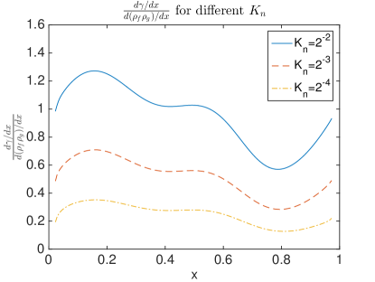
For arbitrary inflow data ϕitalic-ϕ\phi and Dirac delta function δysubscript𝛿𝑦\delta_{y}, as the Knudsen number 𝖪𝗇0𝖪𝗇0\mathsf{Kn}\rightarrow 0, ddxγ𝖪𝗇0dd𝑥subscript𝛾𝖪𝗇0\frac{\mathrm{d}}{\mathrm{d}x}\gamma_{\mathsf{Kn}}\rightarrow 0.

Proof.

Notice that

{g=v𝖪𝗇σaxg+σs0𝖪𝗇2σagf0=v𝖪𝗇σaxf0+σs0𝖪𝗇2σaf0cases𝑔absent𝑣𝖪𝗇subscript𝜎𝑎subscript𝑥𝑔subscript𝜎𝑠0superscript𝖪𝗇2subscript𝜎𝑎𝑔subscript𝑓0absent𝑣𝖪𝗇subscript𝜎𝑎subscript𝑥subscript𝑓0subscript𝜎𝑠0superscript𝖪𝗇2subscript𝜎𝑎subscript𝑓0\begin{cases}g&=\frac{v}{\mathsf{Kn}\sigma_{a}}\partial_{x}g+\frac{\sigma_{s0}}{\mathsf{Kn}^{2}\sigma_{a}}\mathcal{L}g\\ f_{0}&=-\frac{v}{\mathsf{Kn}\sigma_{a}}\partial_{x}f_{0}+\frac{\sigma_{s0}}{\mathsf{Kn}^{2}\sigma_{a}}\mathcal{L}f_{0}\\ \end{cases}

we can derive that

ddxf0gdd𝑥delimited-⟨⟩subscript𝑓0𝑔\displaystyle\frac{\mathrm{d}}{\mathrm{d}x}\langle f_{0}g\rangle =gxf0+f0xgabsentdelimited-⟨⟩𝑔subscript𝑥subscript𝑓0delimited-⟨⟩subscript𝑓0subscript𝑥𝑔\displaystyle=\langle g\partial_{x}f_{0}\rangle+\langle f_{0}\partial_{x}g\rangle
=xf0v𝖪𝗇σaxg+xf0σs0𝖪𝗇2σaggxf0σs0𝖪𝗇2σaabsentdelimited-⟨⟩subscript𝑥subscript𝑓0𝑣𝖪𝗇subscript𝜎𝑎subscript𝑥𝑔delimited-⟨⟩subscript𝑥subscript𝑓0subscript𝜎𝑠0superscript𝖪𝗇2subscript𝜎𝑎delimited-⟨⟩𝑔delimited-⟨⟩𝑔subscript𝑥subscript𝑓0subscript𝜎𝑠0superscript𝖪𝗇2subscript𝜎𝑎\displaystyle=\langle\partial_{x}f_{0}\frac{v}{\mathsf{Kn}\sigma_{a}}\partial_{x}g\rangle+\langle\partial_{x}f_{0}\rangle\frac{\sigma_{s0}}{\mathsf{Kn}^{2}\sigma_{a}}\langle g\rangle-\langle g\partial_{x}f_{0}\rangle\frac{\sigma_{s0}}{\mathsf{Kn}^{2}\sigma_{a}}
+xf0v𝖪𝗇σaxg+f0σs0𝖪𝗇2σaxgf0xgσs0𝖪𝗇2σadelimited-⟨⟩subscript𝑥subscript𝑓0𝑣𝖪𝗇subscript𝜎𝑎subscript𝑥𝑔delimited-⟨⟩subscript𝑓0subscript𝜎𝑠0superscript𝖪𝗇2subscript𝜎𝑎delimited-⟨⟩subscript𝑥𝑔delimited-⟨⟩subscript𝑓0subscript𝑥𝑔subscript𝜎𝑠0superscript𝖪𝗇2subscript𝜎𝑎\displaystyle\quad+\langle-\partial_{x}f_{0}\frac{v}{\mathsf{Kn}\sigma_{a}}\partial_{x}g\rangle+\langle f_{0}\rangle\frac{\sigma_{s0}}{\mathsf{Kn}^{2}\sigma_{a}}\langle\partial_{x}g\rangle-\langle f_{0}\partial_{x}g\rangle\frac{\sigma_{s0}}{\mathsf{Kn}^{2}\sigma_{a}}
=σs0𝖪𝗇2σaddx(f0g)σs0𝖪𝗇2σaddxf0gabsentsubscript𝜎𝑠0superscript𝖪𝗇2subscript𝜎𝑎dd𝑥delimited-⟨⟩subscript𝑓0delimited-⟨⟩𝑔subscript𝜎𝑠0superscript𝖪𝗇2subscript𝜎𝑎dd𝑥delimited-⟨⟩subscript𝑓0𝑔\displaystyle=\frac{\sigma_{s0}}{\mathsf{Kn}^{2}\sigma_{a}}\frac{\mathrm{d}}{\mathrm{d}x}(\langle f_{0}\rangle\langle g\rangle)-\frac{\sigma_{s0}}{\mathsf{Kn}^{2}\sigma_{a}}\frac{\mathrm{d}}{\mathrm{d}x}\langle f_{0}g\rangle

this is equivalent to

ddxf0g=σs0/σa𝖪𝗇2+σs0/σaddx(f0g),dd𝑥delimited-⟨⟩subscript𝑓0𝑔subscript𝜎𝑠0subscript𝜎𝑎superscript𝖪𝗇2subscript𝜎𝑠0subscript𝜎𝑎dd𝑥delimited-⟨⟩subscript𝑓0delimited-⟨⟩𝑔\frac{\mathrm{d}}{\mathrm{d}x}\langle f_{0}g\rangle=\frac{\sigma_{s0}/\sigma_{a}}{\mathsf{Kn}^{2}+\sigma_{s0}/\sigma_{a}}\frac{\mathrm{d}}{\mathrm{d}x}(\langle f_{0}\rangle\langle g\rangle)\,,

therefore we have

ddxγ𝖪𝗇=𝖪𝗇𝖪𝗇2+σs0/σaddx(f0g)0 as 𝖪𝗇0.formulae-sequencedd𝑥subscript𝛾𝖪𝗇𝖪𝗇superscript𝖪𝗇2subscript𝜎𝑠0subscript𝜎𝑎dd𝑥delimited-⟨⟩subscript𝑓0delimited-⟨⟩𝑔0 as 𝖪𝗇0\frac{\mathrm{d}}{\mathrm{d}x}\gamma_{\mathsf{Kn}}=\frac{\mathsf{Kn}}{\mathsf{Kn}^{2}+\sigma_{s0}/\sigma_{a}}\frac{\mathrm{d}}{\mathrm{d}x}(\langle f_{0}\rangle\langle g\rangle)\rightarrow 0\qquad\text{ as }~{}\mathsf{Kn}\rightarrow 0\,.

This proposition indicates that as 𝖪𝗇0𝖪𝗇0\mathsf{Kn}\to 0, whatever boundary condition we provide for f0subscript𝑓0f_{0} and g𝑔g, γ𝖪𝗇subscript𝛾𝖪𝗇\gamma_{\mathsf{Kn}} is going to be flat, and thus not able to distinguish the variation in σssubscript𝜎𝑠\sigma_{s}, making the problem more and more non-injective.

Theorem 6.

When Kundsen number 𝖪𝗇0𝖪𝗇0\mathsf{Kn}\rightarrow 0, solving linear system γ𝖪𝗇,σ~sL2(dx)=bsubscriptsubscript𝛾𝖪𝗇subscript~𝜎𝑠superscript𝐿2d𝑥𝑏\langle\gamma_{\mathsf{Kn}},\tilde{\sigma}_{s}\rangle_{L^{2}(\mathrm{d}{x})}=b is non-injective. More specifically, in the zero limit of 𝖪𝗇𝖪𝗇\mathsf{Kn}, the space spaned by the kernel γ𝖪𝗇subscript𝛾𝖪𝗇\gamma_{\mathsf{Kn}} has finite rank, impossible to reflect full information of σ~ssubscript~𝜎𝑠\tilde{\sigma}_{s}.

Proof.

The non-injectivity of the linear system directly follows from Proposition 2. Moreover, we show in below that the space that γ𝛾\gamma resides in is of low rank in the zero limit of 𝖪𝗇𝖪𝗇\mathsf{Kn}. Let the domain of x𝑥x be xlxxrsubscript𝑥𝑙𝑥subscript𝑥𝑟x_{l}\leq x\leq x_{r} and denote

f0:=ρf,g:=ρg.formulae-sequenceassigndelimited-⟨⟩subscript𝑓0subscript𝜌𝑓assigndelimited-⟨⟩𝑔subscript𝜌𝑔\langle f_{0}\rangle:=\rho_{f},\quad\langle g\rangle:=\rho_{g}\,.

As Knudsen number 𝖪𝗇𝖪𝗇\mathsf{Kn} goes to zero, ρfsubscript𝜌𝑓\rho_{f} and ρgsubscript𝜌𝑔\rho_{g} solves the diffusion equation in the leading order:

ddx(1σs0ddxρf)=σaρf,ddx(1σs0ddxρg)=σaρg,formulae-sequencedd𝑥1subscript𝜎𝑠0𝑑𝑑𝑥subscript𝜌𝑓subscript𝜎𝑎subscript𝜌𝑓dd𝑥1subscript𝜎𝑠0𝑑𝑑𝑥subscript𝜌𝑔subscript𝜎𝑎subscript𝜌𝑔\displaystyle\frac{\mathrm{d}}{\mathrm{d}x}\left(\frac{1}{\sigma_{s0}}\frac{d}{dx}\rho_{f}\right)=\sigma_{a}\rho_{f}\,,\quad\frac{\mathrm{d}}{\mathrm{d}x}\left(\frac{1}{\sigma_{s0}}\frac{d}{dx}\rho_{g}\right)=\sigma_{a}\rho_{g}\,,

with velocity averaged boundary data ξfsubscript𝜉𝑓\xi_{f} and ξgsubscript𝜉𝑔\xi_{g} at only two points: left and right end points. That is,

ρf(xl)=ξfl,ρf(xr)=ξfr;ρg(xl)=ξgl,ρf(xr)=ξgr.formulae-sequencesubscript𝜌𝑓subscript𝑥𝑙subscript𝜉subscript𝑓𝑙formulae-sequencesubscript𝜌𝑓subscript𝑥𝑟subscript𝜉subscript𝑓𝑟formulae-sequencesubscript𝜌𝑔subscript𝑥𝑙subscript𝜉subscript𝑔𝑙subscript𝜌𝑓subscript𝑥𝑟subscript𝜉subscript𝑔𝑟\rho_{f}(x_{l})=\xi_{f_{l}},~{}\rho_{f}(x_{r})=\xi_{f_{r}};\qquad\rho_{g}(x_{l})=\xi_{g_{l}},~{}\rho_{f}(x_{r})=\xi_{g_{r}}\,.

In 1D, there are two Green’s functions:

y(1σs0yG1)=σaG1,G1(x,y=xl)=1,G1(x,y=xr)=0,formulae-sequence𝑦1subscript𝜎𝑠0𝑦subscript𝐺1subscript𝜎𝑎subscript𝐺1formulae-sequencesubscript𝐺1𝑥𝑦subscript𝑥𝑙1subscript𝐺1𝑥𝑦subscript𝑥𝑟0\frac{\partial}{\partial y}\left(\frac{1}{\sigma_{s0}}\frac{\partial}{\partial y}G_{1}\right)=\sigma_{a}G_{1}\,,\quad G_{1}(x,y=x_{l})=1\,,\quad G_{1}(x,y=x_{r})=0\,,

and

y(1σs0yG2)=σaG2,G2(x,y=xl)=0,G2(x,y=xr)=1.formulae-sequence𝑦1subscript𝜎𝑠0𝑦subscript𝐺2subscript𝜎𝑎subscript𝐺2formulae-sequencesubscript𝐺2𝑥𝑦subscript𝑥𝑙0subscript𝐺2𝑥𝑦subscript𝑥𝑟1\frac{\partial}{\partial y}\left(\frac{1}{\sigma_{s0}}\frac{\partial}{\partial y}G_{2}\right)=\sigma_{a}G_{2}\,,\quad G_{2}(x,y=x_{l})=0\,,\quad G_{2}(x,y=x_{r})=1\,.

Then ρfsubscript𝜌𝑓\rho_{f} and ρgsubscript𝜌𝑔\rho_{g} can be written as

ρf=ξflG1(x)+ξfrG2(x);ρg=ξglG1(x)+ξgrG2(x).formulae-sequencesubscript𝜌𝑓subscript𝜉subscript𝑓𝑙subscript𝐺1𝑥subscript𝜉subscript𝑓𝑟subscript𝐺2𝑥subscript𝜌𝑔subscript𝜉subscript𝑔𝑙subscript𝐺1𝑥subscript𝜉subscript𝑔𝑟subscript𝐺2𝑥\rho_{f}=\xi_{f_{l}}G_{1}(x)+\xi_{f_{r}}G_{2}(x);\quad\rho_{g}=\xi_{g_{l}}G_{1}(x)+\xi_{g_{r}}G_{2}(x)\,.

As a result, ρf(x)ρg(x)span{G1(x)2,G1(x)G2(x),G2(x)2}subscript𝜌𝑓𝑥subscript𝜌𝑔𝑥spansubscript𝐺1superscript𝑥2subscript𝐺1𝑥subscript𝐺2𝑥subscript𝐺2superscript𝑥2\rho_{f}(x)\rho_{g}(x)\in\text{span}\{G_{1}(x)^{2},G_{1}(x)G_{2}(x),G_{2}(x)^{2}\}, which means that the function space of ρfρgsubscript𝜌𝑓subscript𝜌𝑔\rho_{f}\rho_{g} is of low rank (rank 3). Combining with Proposition 2, we see that:

ddxγ𝖪𝗇=𝖪𝗇𝖪𝗇2+σs0/σaddx(ρfρg),dd𝑥subscript𝛾𝖪𝗇𝖪𝗇superscript𝖪𝗇2subscript𝜎𝑠0subscript𝜎𝑎dd𝑥subscript𝜌𝑓subscript𝜌𝑔\frac{\mathrm{d}}{\mathrm{d}x}\gamma_{\mathsf{Kn}}=\frac{\mathsf{Kn}}{\mathsf{Kn}^{2}+\sigma_{s0}/\sigma_{a}}\frac{\mathrm{d}}{\mathrm{d}x}\left(\rho_{f}\rho_{g}\right)\,,

meaning ddxγ𝖪𝗇dd𝑥subscript𝛾𝖪𝗇\frac{\mathrm{d}}{\mathrm{d}x}\gamma_{\mathsf{Kn}} is low rank as well. Therefore it is impossible to recover σ~ssubscript~𝜎𝑠\tilde{\sigma}_{s} from the linear mapping γ𝖪𝗇,L2(dx)subscriptsubscript𝛾𝖪𝗇superscript𝐿2d𝑥\langle\gamma_{\mathsf{Kn}},\cdot\rangle_{L^{2}(\mathrm{d}{x})}. ∎

Remark 5.

Theorem 6 coincides with our intuition in Section 1 since when Knudsen number is small, the scattering will dominate absorption as neutron travels through the medium, and the case described here converges to the critical case.

4.3. Ill-conditioning in higher dimensions

In higher dimension, we show that the inverse problem become more and more singular as the Knudsen number approaches zero.

Recall the linear mapping in this scenario:

γ𝖪𝗇,σ~s=b(δy,ϕd),withγ𝖪𝗇=1𝖪𝗇f0gdv,formulae-sequencesubscript𝛾𝖪𝗇subscript~𝜎𝑠𝑏subscript𝛿𝑦subscriptitalic-ϕ𝑑withsubscript𝛾𝖪𝗇1𝖪𝗇subscript𝑓0𝑔differential-d𝑣\langle\gamma_{\mathsf{Kn}},\tilde{\sigma}_{s}\rangle=b(\delta_{y},\phi_{d}),\qquad\text{with}\quad\gamma_{\mathsf{Kn}}=\frac{1}{\mathsf{Kn}}\int\mathcal{L}f_{0}g\mathrm{d}{v}\,,

where f0subscript𝑓0f_{0} and g𝑔g solve (46) (48), respectively. We then investigate the sensitivity of reconstructing σ~ssubscript~𝜎𝑠\tilde{\sigma}_{s}. The main theorem states as follows.

Theorem 7.

Assume that the map from σ~ssubscript~𝜎𝑠\tilde{\sigma}_{s} to b𝑏b is injective. Given an error tolerance δ𝛿\delta on the measurement, the distinguishability coefficient in reconstructing σ~ssubscript~𝜎𝑠\tilde{\sigma}_{s} grows as δ𝛿\delta grows and 𝖪𝗇𝖪𝗇\mathsf{Kn} shrinks. Namely, there exists a constant C𝐶C such that

κs:=supσsΓδσsσ~sL(dx)σ~sL(dx)Cδ𝖪𝗇,when𝖪𝗇1,formulae-sequenceassignsubscript𝜅𝑠subscriptsupremumsubscript𝜎𝑠subscriptΓ𝛿subscriptnormsubscript𝜎𝑠subscript~𝜎𝑠superscript𝐿d𝑥subscriptnormsubscript~𝜎𝑠superscript𝐿d𝑥𝐶𝛿𝖪𝗇much-less-thanwhen𝖪𝗇1\kappa_{s}:=\sup_{\sigma_{s}\in\Gamma_{\delta}}\frac{\|\sigma_{s}-\tilde{\sigma}_{s}\|_{L^{\infty}(\mathrm{d}{x})}}{\|\tilde{\sigma}_{s}\|_{L^{\infty}(\mathrm{d}{x})}}\geq C\frac{\delta}{\mathsf{Kn}},\quad\text{when}\quad\mathsf{Kn}\ll 1\,, (52)

where

Γδ={σ:supϕL(Γ)1,yΩ|γ𝖪𝗇,σL2(dx)b(δy,ϕd)|δ}.subscriptΓ𝛿conditional-set𝜎subscriptsupremumfor-allsubscriptnormitalic-ϕsuperscript𝐿subscriptΓ1for-all𝑦Ωsubscriptsubscript𝛾𝖪𝗇𝜎superscript𝐿2d𝑥𝑏subscript𝛿𝑦subscriptitalic-ϕ𝑑𝛿\Gamma_{\delta}=\{\sigma:\sup_{\begin{subarray}{c}\forall\|\phi\|_{L^{\infty}(\Gamma_{-})}\leq 1,\\ \forall y\in\partial\Omega\end{subarray}}|\langle\gamma_{\mathsf{Kn}}\,,\sigma\rangle_{L^{2}(\mathrm{d}{x})}-b(\delta_{y},\phi_{d})|\leq\delta\}\,.
Proof.

When 𝖪𝗇𝖪𝗇\mathsf{Kn} is small, we decompose f0subscript𝑓0f_{0} and g𝑔g into a layer part that accounts for the boundary layer supported in the vicinity of the boundary ΩΩ\partial\Omega with 𝒪(𝖪𝗇)𝒪𝖪𝗇\mathcal{O}(\mathsf{Kn}) width and an interior part:

f0=fL+fI,g=gL+gI.formulae-sequencesubscript𝑓0subscript𝑓𝐿subscript𝑓𝐼𝑔subscript𝑔𝐿subscript𝑔𝐼f_{0}=f_{L}+f_{I},\quad g=g_{L}+g_{I}\,.

Decompose also γ𝖪𝗇subscript𝛾𝖪𝗇\gamma_{\mathsf{Kn}} as γ𝖪𝗇=(γ𝖪𝗇)L+(γ𝖪𝗇)Isubscript𝛾𝖪𝗇subscriptsubscript𝛾𝖪𝗇𝐿subscriptsubscript𝛾𝖪𝗇𝐼\gamma_{\mathsf{Kn}}=\left(\gamma_{\mathsf{Kn}}\right)_{L}+\left(\gamma_{\mathsf{Kn}}\right)_{I}, then we examine the interior part (γ𝖪𝗇)Isubscriptsubscript𝛾𝖪𝗇𝐼(\gamma_{\mathsf{Kn}})_{I} by means of fIsubscript𝑓𝐼f_{I} and gIsubscript𝑔𝐼g_{I}. Upon asymptotic expansion, the interior solutions fIsubscript𝑓𝐼f_{I} and gIsubscript𝑔𝐼g_{I} are approximated as follows

fIsubscript𝑓𝐼\displaystyle f_{I} =\displaystyle= ρf𝖪𝗇σs0vxρf+𝖪𝗇2f2,subscript𝜌𝑓𝖪𝗇subscript𝜎𝑠0𝑣subscript𝑥subscript𝜌𝑓superscript𝖪𝗇2subscript𝑓2\displaystyle\rho_{f}-\frac{\mathsf{Kn}}{\sigma_{s0}}v\cdot\nabla_{x}\rho_{f}+\mathsf{Kn}^{2}f_{2}\,,
gIsubscript𝑔𝐼\displaystyle g_{I} =\displaystyle= ρg+𝖪𝗇σs0vxρg+𝖪𝗇2g2,subscript𝜌𝑔𝖪𝗇subscript𝜎𝑠0𝑣subscript𝑥subscript𝜌𝑔superscript𝖪𝗇2subscript𝑔2\displaystyle\rho_{g}+\frac{\mathsf{Kn}}{\sigma_{s0}}v\cdot\nabla_{x}\rho_{g}+\mathsf{Kn}^{2}g_{2}\,,

hence,

(γ𝖪𝗇)Isubscriptsubscript𝛾𝖪𝗇𝐼\displaystyle(\gamma_{\mathsf{Kn}})_{I} =\displaystyle= 1𝖪𝗇(fIgIfIgI)1𝖪𝗇delimited-⟨⟩subscript𝑓𝐼delimited-⟨⟩subscript𝑔𝐼delimited-⟨⟩subscript𝑓𝐼subscript𝑔𝐼\displaystyle\frac{1}{\mathsf{Kn}}(\langle f_{I}\rangle\langle g_{I}\rangle-\langle f_{I}g_{I}\rangle) (53)
=\displaystyle= 1𝖪𝗇{(ρf𝖪𝗇2f2)(ρg+𝖪𝗇2g2)\displaystyle\frac{1}{\mathsf{Kn}}\left\{(\rho_{f}-\mathsf{Kn}^{2}\langle f_{2}\rangle)(\rho_{g}+\mathsf{Kn}^{2}\langle g_{2}\rangle)\right.
(ρf𝖪𝗇σs0vxρf+𝖪𝗇2f2)(ρg𝖪𝗇σs0vxρg+𝖪𝗇2g2)}\displaystyle\qquad\left.-\left\langle\left(\rho_{f}-\frac{\mathsf{Kn}}{\sigma_{s0}}v\cdot\nabla_{x}\rho_{f}+\mathsf{Kn}^{2}f_{2}\right)\left(\rho_{g}-\frac{\mathsf{Kn}}{\sigma_{s0}}v\cdot\nabla_{x}\rho_{g}+\mathsf{Kn}^{2}g_{2}\right)\right\rangle\right\}
=\displaystyle= 𝖪𝗇σs02(vxρf)(vxρg)+𝒪(𝖪𝗇2)𝖪𝗇superscriptsubscript𝜎𝑠02delimited-⟨⟩𝑣subscript𝑥subscript𝜌𝑓𝑣subscript𝑥subscript𝜌𝑔𝒪superscript𝖪𝗇2\displaystyle-\frac{\mathsf{Kn}}{\sigma_{s0}^{2}}\langle(v\cdot\nabla_{x}\rho_{f})(v\cdot\nabla_{x}\rho_{g})\rangle+\mathcal{O}(\mathsf{Kn}^{2})
=\displaystyle= 𝖪𝗇σs02Cxρfxρg+𝒪(𝖪𝗇2),𝖪𝗇superscriptsubscript𝜎𝑠02𝐶subscript𝑥subscript𝜌𝑓subscript𝑥subscript𝜌𝑔𝒪superscript𝖪𝗇2\displaystyle-\frac{\mathsf{Kn}}{\sigma_{s0}^{2}}C\nabla_{x}\rho_{f}\cdot\nabla_{x}\rho_{g}+\mathcal{O}(\mathsf{Kn}^{2})\,,

where C𝐶C is a constant depending on the dimension of the problem. Now consider c(x)𝑐𝑥c(x) such that it vanishes in the boundary layer and that

|γ𝖪𝗇,cL2(dx)|δ,subscriptsubscript𝛾𝖪𝗇𝑐superscript𝐿2d𝑥𝛿|\langle\gamma_{\mathsf{Kn}},c\rangle_{L^{2}(\mathrm{d}{x})}|\leq\delta\,,

then one certainly has

σs(x)=c(x)+σ~s(x)Γδ.subscript𝜎𝑠𝑥𝑐𝑥subscript~𝜎𝑠𝑥subscriptΓ𝛿\sigma_{s}(x)=c(x)+\tilde{\sigma}_{s}(x)\in\Gamma_{\delta}\,.

Since γ𝖪𝗇,cL2(dx)=(γ𝖪𝗇)I,cIL2(dx)=𝖪𝗇σs02Cxρfxρg,cIL2(dx)+𝒪(𝖪𝗇2)subscriptsubscript𝛾𝖪𝗇𝑐superscript𝐿2d𝑥subscriptsubscriptsubscript𝛾𝖪𝗇𝐼subscript𝑐𝐼superscript𝐿2d𝑥subscript𝖪𝗇superscriptsubscript𝜎𝑠02𝐶subscript𝑥subscript𝜌𝑓subscript𝑥subscript𝜌𝑔subscript𝑐𝐼superscript𝐿2d𝑥𝒪superscript𝖪𝗇2\langle\gamma_{\mathsf{Kn}},c\rangle_{L^{2}(\mathrm{d}{x})}=\langle(\gamma_{\mathsf{Kn}})_{I},c_{I}\rangle_{L^{2}(\mathrm{d}{x})}=\langle-\frac{\mathsf{Kn}}{\sigma_{s0}^{2}}C\nabla_{x}\rho_{f}\cdot\nabla_{x}\rho_{g},c_{I}\rangle_{L^{2}(\mathrm{d}{x})}+\mathcal{O}(\mathsf{Kn}^{2}), we immediately have

cL(dx)𝒪(δ𝖪𝗇),similar-tosubscriptnorm𝑐superscript𝐿d𝑥𝒪𝛿𝖪𝗇\|c\|_{L^{\infty}(\mathrm{d}{x})}\sim\mathcal{O}\left(\frac{\delta}{\mathsf{Kn}}\right)\,,

which implies that

κsCδ𝖪𝗇,for some constantC.subscript𝜅𝑠𝐶𝛿𝖪𝗇for some constant𝐶\kappa_{s}\geq C\frac{\delta}{\mathsf{Kn}}\,,\quad\text{for some constant}\quad C\,.

Remark 6.

Notice that in the expression (53), the leading term in γ𝛾\gamma has the structure of xρfxρgsubscript𝑥subscript𝜌𝑓subscript𝑥subscript𝜌𝑔\nabla_{x}\rho_{f}\cdot\nabla_{x}\rho_{g}, where ρfsubscript𝜌𝑓\rho_{f} and ρgsubscript𝜌𝑔\rho_{g} solve the diffusion equation with corresponding boundary condition, which has a Green’s function formation. Therefore, one can show that it is asymptotically “low rank” in the sense that one can find a nonzero c(x)𝑐𝑥c(x) such that

xρfxρgcdx=𝒪(𝖪𝗇).subscript𝑥subscript𝜌𝑓subscript𝑥subscript𝜌𝑔𝑐d𝑥𝒪𝖪𝗇\int\nabla_{x}\rho_{f}\cdot\nabla_{x}\rho_{g}c\mathrm{d}{x}=\mathcal{O}(\mathsf{Kn})\,.

Details follow the argument in the proof of Theorem 2 .

5. Numerical test

In this section, we conduct a few numerical experiments in 1D to check the conditioning of the inverse problem, and show that it degrades when 𝖪𝗇𝖪𝗇\mathsf{Kn} goes to zero, as indicated by the theory above. More specifically, we check the variation of γ(x;δy,ϕ)𝛾𝑥subscript𝛿𝑦italic-ϕ\gamma(x;\delta_{y},\phi) in x𝑥x and examine the singular values of the matrix 𝖠𝖠\mathsf{A}, whose element takes values 𝖠pi=γ(xi;δyk,ϕd)subscript𝖠𝑝𝑖𝛾subscript𝑥𝑖subscript𝛿subscript𝑦𝑘subscriptitalic-ϕ𝑑\mathsf{A}_{pi}=\gamma(x_{i};\delta_{y_{k}},\phi_{d}) with (k,d)=p𝑘𝑑𝑝(k,d)=p.

Recall the definition of γ(x;δyk,ϕd)𝛾𝑥subscript𝛿subscript𝑦𝑘subscriptitalic-ϕ𝑑\gamma(x;\delta_{y_{k}},\phi_{d}) in (23) and (50), one needs to solve the forward problems for f0subscript𝑓0f_{0} and g𝑔g with boundary conditions ϕdsubscriptitalic-ϕ𝑑\phi_{d}, and δysubscript𝛿𝑦\delta_{y}, respectively. The forward solver we adopt is the fully implicit solver [24] with Generalized minimal residual method (GMRES) under a tolerance of 1010superscript101010^{-10}. For all the examples below, the spatial domain is chosen as Ω=[0,1]Ω01\Omega=[0,1] and discretized with Nx=200subscript𝑁𝑥200N_{x}=200 uniformly distributed nodes. We also sample Nv=80subscript𝑁𝑣80N_{v}=80 grid points in the velocity domain 𝒮=[1,1]𝒮11\mathcal{S}=[-1,1]. Note that for the 𝖪𝗇𝖪𝗇\mathsf{Kn} we considered here, the spatial mesh is fine enough to resolve the boundary layers.

Now we need to decide the boundary condition f0|Γ=ϕd(x,v)evaluated-atsubscript𝑓0subscriptΓsubscriptitalic-ϕ𝑑𝑥𝑣f_{0}|_{\Gamma_{-}}=\phi_{d}(x,v) and g|Γ=δy(x)evaluated-at𝑔subscriptΓsubscript𝛿𝑦𝑥g|_{\Gamma_{-}}=\delta_{y}(x) such that we extract the most information from f0subscript𝑓0f_{0} and g𝑔g. Since f0subscript𝑓0f_{0} solves a linear equation, we can set delta functions as its inflow data, i.e.,

ϕd(0,v)=δ(vvd),vd>0,d=1,,40;ϕd(1,v)=δ(vvd),vd<0,d=41,,80.formulae-sequencesubscriptitalic-ϕ𝑑0𝑣𝛿𝑣subscript𝑣𝑑formulae-sequencesubscript𝑣𝑑0formulae-sequence𝑑140formulae-sequencesubscriptitalic-ϕ𝑑1𝑣𝛿𝑣subscript𝑣𝑑formulae-sequencesubscript𝑣𝑑0𝑑4180\phi_{d}(0,v)=\delta(v-v_{d}),\quad v_{d}>0,\quad d=1,\cdots,40\,;\qquad\phi_{d}(1,v)=\delta(v-v_{d}),\quad v_{d}<0,\quad d=41,\cdots,80\,.

The boundary condition for g𝑔g is easier to set up. Note that in 1D, there are only two boundary points, x=0𝑥0x=0 and x=1𝑥1x=1, therefore, the boundary for g𝑔g reads

δy1=δ(x0),δy2=δ(x1).formulae-sequencesubscript𝛿subscript𝑦1𝛿𝑥0subscript𝛿subscript𝑦2𝛿𝑥1\delta_{y_{1}}=\delta(x-0),\quad\delta_{y_{2}}=\delta(x-1)\,.

Then the associated matrix is of size 𝖠160×200𝖠superscript160200\mathsf{A}\in\mathbb{R}^{160\times 200}.

5.1. Recover Absorption Coefficient

The first test addresses the problem of recovering σasubscript𝜎𝑎\sigma_{a}. Here the background absorption is set to be σs=1+11.5+sin(2πx)subscript𝜎𝑠111.52𝜋𝑥\sigma_{s}=1+\frac{1}{1.5+\sin(2\pi x)} and the scattering coefficient takes the form σa0=4+12sin(4πx)subscript𝜎𝑎04124𝜋𝑥\sigma_{a0}=4+\frac{1}{2}\sin(4\pi x). Here

𝖠pi=𝖪𝗇g(xi,v;δyk)f0(x,v;ϕd)dv,p=(d,k).formulae-sequencesubscript𝖠𝑝𝑖𝖪𝗇𝑔subscript𝑥𝑖𝑣subscript𝛿subscript𝑦𝑘subscript𝑓0𝑥𝑣subscriptitalic-ϕ𝑑differential-d𝑣𝑝𝑑𝑘\mathsf{A}_{pi}=\mathsf{Kn}\int g(x_{i},v;\delta_{y_{k}})f_{0}(x,v;\phi_{d})\mathrm{d}{v},\quad p=(d,k)\,. (54)

As predicted in Theorem 3, in 1D, the matrix 𝖠𝖠\mathsf{A} is approximately low rank with rank 3, which indicates that its singular value decays to zero quickly. This is demonstrated in Fig. 1, wherein we plot the singular values for a variety of 𝖪𝗇𝖪𝗇\mathsf{Kn}. It is easy to see that only three singular values stand out, coincide with the rank 3 argument. And the difference between the first three singular values with the rest are more pronounced with smaller 𝖪𝗇𝖪𝗇\mathsf{Kn}.

Refer to caption
Figure 1. Plots of the singular values for γ𝖪𝗇subscript𝛾𝖪𝗇\gamma_{\mathsf{Kn}} in (23) (discrete form is (54)) when 𝖪𝗇=22,23𝖪𝗇superscript22superscript23\mathsf{Kn}=2^{-2},2^{-3} and 24superscript242^{-4}.

Moreover, we see in the proof of Theorem 2 (see equation (31)) that γ𝖪𝗇𝖪𝗇ρfρgsubscript𝛾𝖪𝗇𝖪𝗇subscript𝜌𝑓subscript𝜌𝑔\gamma_{\mathsf{Kn}}\approx\mathsf{Kn}\rho_{f}\rho_{g} for small 𝖪𝗇𝖪𝗇\mathsf{Kn}, which lives in a space spanned by G12subscriptsuperscript𝐺21G^{2}_{1}, G22subscriptsuperscript𝐺22G^{2}_{2} and G1G2subscript𝐺1subscript𝐺2G_{1}G_{2} with G1,2subscript𝐺12G_{1,2} standing for the Green’s functions. The plots in 2 show the first three eigenvectors of 𝖠𝖠\mathsf{A} as 𝖪𝗇0𝖪𝗇0\mathsf{Kn}\to 0.

Refer to caption
Refer to caption
Refer to caption
Figure 2. Plots of the singular vectors for 𝖠𝖠\mathsf{A} when 𝖪𝗇=22,23𝖪𝗇superscript22superscript23\mathsf{Kn}=2^{-2},2^{-3} and 24superscript242^{-4}. It can be seen that the first two eigenvectors are almost symmetric to each other.

5.2. Recover Scattering Coefficient

In the second test, we aim to recover σssubscript𝜎𝑠\sigma_{s}. Here

𝖠pi=1𝖪𝗇g(xi,v,δyk)f0(xi,v;ϕd)dv,p=(k,d).formulae-sequencesubscript𝖠𝑝𝑖1𝖪𝗇𝑔subscript𝑥𝑖𝑣subscript𝛿subscript𝑦𝑘subscript𝑓0subscript𝑥𝑖𝑣subscriptitalic-ϕ𝑑differential-d𝑣𝑝𝑘𝑑\mathsf{A}_{pi}=\frac{1}{\mathsf{Kn}}\int g(x_{i},v,\delta_{y_{k}})\mathcal{L}f_{0}(x_{i},v;\phi_{d})\mathrm{d}v,\quad p=(k,d)\,.

We first compute γ𝖪𝗇subscript𝛾𝖪𝗇\gamma_{\mathsf{Kn}} (stored in 𝖠𝖠\mathsf{A}) with σs0=1+11.5+sin(2πx)subscript𝜎𝑠0111.52𝜋𝑥\sigma_{s0}=1+\frac{1}{1.5+\sin(2\pi x)} and σa=0subscript𝜎𝑎0\sigma_{a}=0. It is seen from Proposition 1 that γ𝖪𝗇subscript𝛾𝖪𝗇\gamma_{\mathsf{Kn}} stays unchanged in x𝑥x direction, i.e., dγ𝖪𝗇dx=0dsubscript𝛾𝖪𝗇d𝑥0\frac{\mathrm{d}\gamma_{\mathsf{Kn}}}{\mathrm{d}x}=0. To show this, we plot the matrix 𝖠𝖠\mathsf{A} in Fig. 3 and see that the entire matrix is roughly flat in x𝑥x direction.

Refer to caption
Figure 3. To recover the scattering coefficient when σa=0subscript𝜎𝑎0\sigma_{a}=0, the problem is expected to be ill-posed with γ𝖪𝗇subscript𝛾𝖪𝗇\gamma_{\mathsf{Kn}} being flat in x𝑥x. We here plot γ𝖪𝗇=1𝖪𝗇[f0]gdvsubscript𝛾𝖪𝗇1𝖪𝗇delimited-[]subscript𝑓0𝑔differential-d𝑣\gamma_{\mathsf{Kn}}=\frac{1}{\mathsf{Kn}}\int\mathcal{L}[f_{0}]g\mathrm{d}{v} with 𝖪𝗇=1𝖪𝗇1\mathsf{Kn}=1, for various of ϕdsubscriptitalic-ϕ𝑑\phi_{d} and δysubscript𝛿𝑦\delta_{y} as the boundary condition for g𝑔g and f0subscript𝑓0f_{0}.

Next we consider the case when σasubscript𝜎𝑎\sigma_{a} is nontrivial: σa=24(4+12sin(4πx))subscript𝜎𝑎superscript244124𝜋𝑥\sigma_{a}=2^{-4}(4+\frac{1}{2}\sin(4\pi x)), and σs0=124(1+11.5+sin(2πx))subscript𝜎𝑠01superscript24111.52𝜋𝑥\sigma_{s0}=\frac{1}{2^{-4}}(1+\frac{1}{1.5+\sin(2\pi x)}). As predicted in Proposition 2, dγ𝖪𝗇dx𝖪𝗇dρfρgdx0similar-todsubscript𝛾𝖪𝗇d𝑥𝖪𝗇dsubscript𝜌𝑓subscript𝜌𝑔d𝑥0\frac{\mathrm{d}\gamma_{\mathsf{Kn}}}{\mathrm{d}x}\sim\mathsf{Kn}\frac{\mathrm{d}\rho_{f}\rho_{g}}{\mathrm{d}x}\to 0 as 𝖪𝗇0𝖪𝗇0\mathsf{Kn}\to 0, and this is demonstrated in Fig. 4, where we plot dγ𝖪𝗇/dxdρfρg/dxdsubscript𝛾𝖪𝗇d𝑥dsubscript𝜌𝑓subscript𝜌𝑔d𝑥\frac{\mathrm{d}\gamma_{\mathsf{Kn}}/\mathrm{d}x}{\mathrm{d}\rho_{f}\rho_{g}/\mathrm{d}x}. As 𝖪𝗇𝖪𝗇\mathsf{Kn} decreases by 1/2121/2, the ratio decrease by 1/2121/2 as well.

Refer to caption
Figure 4. dγ/dxd(ρfρg)/dxd𝛾d𝑥dsubscript𝜌𝑓subscript𝜌𝑔d𝑥\frac{\mathrm{d}\gamma/\mathrm{d}x}{\mathrm{d}(\rho_{f}\rho_{g})/\mathrm{d}x}. The plot shows that the ratio is indeed at the order 𝖪𝗇𝖪𝗇\mathsf{Kn} in the zero limit of 𝖪𝗇𝖪𝗇\mathsf{Kn}, as predicted.

In the end we test the singular value decay of 𝖠Isubscript𝖠𝐼\mathsf{A}_{I}, the interior part of 𝖠𝖠\mathsf{A}. As 𝖪𝗇0𝖪𝗇0\mathsf{Kn}\rightarrow 0, we expect that its element γ𝖪𝗇𝖪𝗇xρfxρgsubscript𝛾𝖪𝗇𝖪𝗇subscript𝑥subscript𝜌𝑓subscript𝑥subscript𝜌𝑔\gamma_{\mathsf{Kn}}\approx\mathsf{Kn}\nabla_{x}\rho_{f}\cdot\nabla_{x}\rho_{g} (see equation (53)), and thus 𝖠Isubscript𝖠𝐼\mathsf{A}_{I} is a low rank matrix. We plot the singular values Fig. 5, and as before, only the first three singular values dominates, and the rest vanishes at the order of 𝖪𝗇𝖪𝗇\mathsf{Kn}.

Refer to caption
Figure 5. To recover σssubscript𝜎𝑠\sigma_{s}, we plot the first few singular values of 𝖠𝖠\mathsf{A} in the interior with 𝖪𝗇=22,23𝖪𝗇superscript22superscript23\mathsf{Kn}=2^{-2},2^{-3} and 24superscript242^{-4}. As 𝖪𝗇0𝖪𝗇0\mathsf{Kn}\to 0, the problem becomes more and more singular.

We also show that for small 𝖪𝗇𝖪𝗇\mathsf{Kn}, γ𝖪𝗇𝖪𝗇xρfxρgsubscript𝛾𝖪𝗇𝖪𝗇subscript𝑥subscript𝜌𝑓subscript𝑥subscript𝜌𝑔\gamma_{\mathsf{Kn}}\approx\mathsf{Kn}\nabla_{x}\rho_{f}\cdot\nabla_{x}\rho_{g}, which lives in a space spanned by (xG1)2superscriptsubscript𝑥subscript𝐺12(\partial_{x}G_{1})^{2}, (xG2)2superscriptsubscript𝑥subscript𝐺22(\partial_{x}G_{2})^{2} and xG1xG2subscript𝑥subscript𝐺1subscript𝑥subscript𝐺2\partial_{x}G_{1}\partial_{x}G_{2} with G1,2subscript𝐺12G_{1,2} standing for the Green’s functions. The plots in 6 show the first three eigenvectors of 𝖠𝖠\mathsf{A} as 𝖪𝗇0𝖪𝗇0\mathsf{Kn}\to 0.

Refer to caption
Refer to caption
Refer to caption
Figure 6. Plots of the singular vectors for 𝖠Isubscript𝖠𝐼\mathsf{A}_{I} when 𝖪𝗇=22,23𝖪𝗇superscript22superscript23\mathsf{Kn}=2^{-2},2^{-3} and 24superscript242^{-4}. It can be seen that the first two eigenvectors are almost symmetric to each other.

6. Appendix

Appendix I: Rank of matrix 𝖠I0superscriptsubscript𝖠𝐼0\mathsf{A}_{I}^{0} Here we examine the rank of matrix 𝖠I0superscriptsubscript𝖠𝐼0\mathsf{A}_{I}^{0}. We show below that it has rank less than 4 in 1D, but not necessarily low rank in higher dimensions. Denote

ρ𝐟=(ρf(x1),ρf(x2),ρf(xNx)),ρ𝐠=(ρg(x1),ρg(x2),,ρg(xNx))formulae-sequencesubscript𝜌𝐟subscript𝜌𝑓subscript𝑥1subscript𝜌𝑓subscript𝑥2subscript𝜌𝑓subscript𝑥subscript𝑁𝑥subscript𝜌𝐠subscript𝜌𝑔subscript𝑥1subscript𝜌𝑔subscript𝑥2subscript𝜌𝑔subscript𝑥subscript𝑁𝑥\mathbf{\rho_{f}}=(\rho_{f}(x_{1}),\rho_{f}(x_{2}),\cdots\rho_{f}(x_{N_{x}})),\quad\mathbf{\rho_{g}}=(\rho_{g}(x_{1}),\rho_{g}(x_{2}),\cdots,\rho_{g}(x_{N_{x}}))\,

as the solutions to the discrete form of equations (29) (30):

ρ𝐟=𝖡1ξ,ρ𝐠=𝖡1δ𝐲,formulae-sequencesubscript𝜌𝐟superscript𝖡1𝜉subscript𝜌𝐠superscript𝖡1subscript𝛿𝐲\mathbf{\rho_{f}}=\mathsf{B}^{-1}\mathbf{\xi},\quad\mathbf{\rho_{g}}=\mathsf{B}^{-1}\mathbf{\delta_{y}}\,,

where 𝖡Nx×Nxsubscript𝖡𝑁𝑥𝑁𝑥\mathsf{B}_{Nx\times Nx} is the discrete version of operator Cxxσa0𝐶subscript𝑥subscript𝑥subscript𝜎𝑎0C\nabla_{x}\cdot\nabla_{x}-\sigma_{a0}. Write 𝖡1=(bij)Nx×Nxsuperscript𝖡1subscriptsubscript𝑏𝑖𝑗subscript𝑁𝑥subscript𝑁𝑥\mathsf{B}^{-1}=(b_{ij})_{N_{x}\times N_{x}}, and recall that the entries of 𝖠I0superscriptsubscript𝖠𝐼0\mathsf{A}_{I}^{0} is (41), we have

𝖠I0=((j=1Nxb1jξj(1))(j=1Nxb1jδ𝐲𝐣(𝟏))w1(j=1NxbNxjξj(1))(j=1NxbNxjδ𝐲𝐣(𝟏))wNx(j=1Nxb1jξj(2))(j=1Nxb1jδ𝐲𝐣(𝟐))w1(j=1NxbNxjξj(2))(j=1NxbNxjδ𝐲𝐣(𝟐))wNx(j=1Nxb1jξj(Np))(j=1Nxb1jδ𝐲𝐣(𝐍𝐩))w1(j=1NxbNxjξj(Np))(j=1NxbNxjδ𝐲𝐣(𝐍𝐩))wNx),superscriptsubscript𝖠𝐼0superscriptsubscript𝑗1subscript𝑁𝑥subscript𝑏1𝑗superscriptsubscript𝜉𝑗1superscriptsubscript𝑗1subscript𝑁𝑥subscript𝑏1𝑗superscriptsubscript𝛿subscript𝐲𝐣1subscript𝑤1superscriptsubscript𝑗1subscript𝑁𝑥subscript𝑏subscript𝑁𝑥𝑗superscriptsubscript𝜉𝑗1superscriptsubscript𝑗1subscript𝑁𝑥subscript𝑏subscript𝑁𝑥𝑗superscriptsubscript𝛿subscript𝐲𝐣1subscript𝑤subscript𝑁𝑥superscriptsubscript𝑗1subscript𝑁𝑥subscript𝑏1𝑗superscriptsubscript𝜉𝑗2superscriptsubscript𝑗1subscript𝑁𝑥subscript𝑏1𝑗superscriptsubscript𝛿subscript𝐲𝐣2subscript𝑤1superscriptsubscript𝑗1subscript𝑁𝑥subscript𝑏subscript𝑁𝑥𝑗superscriptsubscript𝜉𝑗2superscriptsubscript𝑗1subscript𝑁𝑥subscript𝑏subscript𝑁𝑥𝑗superscriptsubscript𝛿subscript𝐲𝐣2subscript𝑤subscript𝑁𝑥superscriptsubscript𝑗1subscript𝑁𝑥subscript𝑏1𝑗superscriptsubscript𝜉𝑗subscript𝑁𝑝superscriptsubscript𝑗1subscript𝑁𝑥subscript𝑏1𝑗superscriptsubscript𝛿subscript𝐲𝐣subscript𝐍𝐩subscript𝑤1superscriptsubscript𝑗1subscript𝑁𝑥subscript𝑏subscript𝑁𝑥𝑗superscriptsubscript𝜉𝑗subscript𝑁𝑝superscriptsubscript𝑗1subscript𝑁𝑥subscript𝑏subscript𝑁𝑥𝑗superscriptsubscript𝛿subscript𝐲𝐣subscript𝐍𝐩subscript𝑤subscript𝑁𝑥\mathsf{A}_{I}^{0}=\left(\begin{array}[]{cccc}\left(\sum_{j=1}^{N_{x}}b_{1j}\xi_{j}^{(1)}\right)\left(\sum_{j=1}^{N_{x}}b_{1j}\mathbf{\delta_{y_{j}}^{(1)}}\right)w_{1}&\cdots&\cdots&\left(\sum_{j=1}^{N_{x}}b_{N_{x}j}\xi_{j}^{(1)}\right)\left(\sum_{j=1}^{N_{x}}b_{N_{x}j}\mathbf{\delta_{y_{j}}^{(1)}}\right)w_{N_{x}}\\ \left(\sum_{j=1}^{N_{x}}b_{1j}\xi_{j}^{(2)}\right)\left(\sum_{j=1}^{N_{x}}b_{1j}\mathbf{\delta_{y_{j}}^{(2)}}\right)w_{1}&\cdots&\cdots&\left(\sum_{j=1}^{N_{x}}b_{N_{x}j}\xi_{j}^{(2)}\right)\left(\sum_{j=1}^{N_{x}}b_{N_{x}j}\mathbf{\delta_{y_{j}}^{(2)}}\right)w_{N_{x}}\\ \cdots&\cdots&\cdots&\cdots\\ \left(\sum_{j=1}^{N_{x}}b_{1j}\xi_{j}^{(N_{p})}\right)\left(\sum_{j=1}^{N_{x}}b_{1j}\mathbf{\delta_{y_{j}}^{(N_{p})}}\right)w_{1}&\cdots&\cdots&\left(\sum_{j=1}^{N_{x}}b_{N_{x}j}\xi_{j}^{(N_{p})}\right)\left(\sum_{j=1}^{N_{x}}b_{N_{x}j}\mathbf{\delta_{y_{j}}^{(N_{p})}}\right)w_{N_{x}}\end{array}\right)\,,

Here without abuse of notation, we still the denote number of interior points Nxsubscript𝑁𝑥N_{x}.

Then in 1D, since we only have two boundary points, Ny=2subscript𝑁𝑦2N_{y}=2, and ξj(l)=0superscriptsubscript𝜉𝑗𝑙0\xi_{j}^{(l)}=0 for all j1𝑗1j\neq 1 or Nxsubscript𝑁𝑥N_{x}, and l=1,2,,Nϕ𝑙12subscript𝑁italic-ϕl=1,2,\cdots,N_{\phi}. Therefore, 𝖠I0superscriptsubscript𝖠𝐼0\mathsf{A}_{I}^{0} can be simplified to

𝖠I0superscriptsubscript𝖠𝐼0\displaystyle\mathsf{A}_{I}^{0} =\displaystyle= (ξ1(1)ξ1(Nϕ)00)(b112b212bNx12b112b212bNx120)(w1wNx)matrixsuperscriptsubscript𝜉11missing-subexpressionmissing-subexpressionmissing-subexpressionmissing-subexpressionmissing-subexpressionmissing-subexpressionmissing-subexpressionmissing-subexpressionmissing-subexpressionsuperscriptsubscript𝜉1subscript𝑁italic-ϕmissing-subexpressionmissing-subexpressionmissing-subexpressionmissing-subexpressionmissing-subexpression0missing-subexpressionmissing-subexpressionmissing-subexpressionmissing-subexpressionmissing-subexpressionmissing-subexpressionmissing-subexpressionmissing-subexpressionmissing-subexpressionmissing-subexpressionmissing-subexpressionmissing-subexpression0matrixsuperscriptsubscript𝑏112superscriptsubscript𝑏212superscriptsubscript𝑏subscript𝑁𝑥12superscriptsubscript𝑏112superscriptsubscript𝑏212superscriptsubscript𝑏subscript𝑁𝑥12missing-subexpressionmissing-subexpressionmissing-subexpressionmissing-subexpressionmissing-subexpressionmissing-subexpressionmissing-subexpressionmissing-subexpressionmissing-subexpressionmissing-subexpressionmissing-subexpressionmissing-subexpression0missing-subexpressionmissing-subexpressionmatrixsubscript𝑤1missing-subexpressionmissing-subexpressionmissing-subexpressionmissing-subexpressionmissing-subexpressionmissing-subexpressionsubscript𝑤subscript𝑁𝑥\displaystyle\begin{pmatrix}\xi_{1}^{(1)}&&&\\ &\ddots&&&\\ &&\xi_{1}^{(N_{\phi})}&&\\ &&&0&&\\ &&&&\ddots&\\ &&&&&0\\ \end{pmatrix}\begin{pmatrix}b_{11}^{2}&b_{21}^{2}&\cdots&\cdots&b_{N_{x}1}^{2}\\ \vdots&\vdots&\vdots&\vdots&\vdots\\ b_{11}^{2}&b_{21}^{2}&\cdots&\cdots&b_{N_{x}1}^{2}\\ &&&&\\ &&&&\\ &&0&&\\ &&&&\end{pmatrix}\begin{pmatrix}w_{1}&&\\ &\ddots&\\ &&w_{N_{x}}\\ \end{pmatrix}
+\displaystyle+ (ξNx(1)ξNx(Nϕ)ξ1(Nϕ+1)ξ1(2Nϕ))(b11b1Nxb21b2NxbNx1bNxNxb11b1Nxb21b2NxbNx1bNxNxb11b1Nxb21b2NxbNx1bNxNxb11b1Nxb21b2NxbNx1bNxNx)(w1wNx)matrixsuperscriptsubscript𝜉subscript𝑁𝑥1missing-subexpressionmissing-subexpressionmissing-subexpressionmissing-subexpressionmissing-subexpressionmissing-subexpressionmissing-subexpressionmissing-subexpressionmissing-subexpressionsuperscriptsubscript𝜉subscript𝑁𝑥subscript𝑁italic-ϕmissing-subexpressionmissing-subexpressionmissing-subexpressionmissing-subexpressionmissing-subexpressionsuperscriptsubscript𝜉1subscript𝑁italic-ϕ1missing-subexpressionmissing-subexpressionmissing-subexpressionmissing-subexpressionmissing-subexpressionmissing-subexpressionmissing-subexpressionmissing-subexpressionmissing-subexpressionmissing-subexpressionmissing-subexpressionmissing-subexpressionsuperscriptsubscript𝜉12subscript𝑁italic-ϕmatrixsubscript𝑏11subscript𝑏1subscript𝑁𝑥subscript𝑏21subscript𝑏2subscript𝑁𝑥subscript𝑏subscript𝑁𝑥1subscript𝑏subscript𝑁𝑥subscript𝑁𝑥subscript𝑏11subscript𝑏1subscript𝑁𝑥subscript𝑏21subscript𝑏2subscript𝑁𝑥subscript𝑏subscript𝑁𝑥1subscript𝑏subscript𝑁𝑥subscript𝑁𝑥subscript𝑏11subscript𝑏1subscript𝑁𝑥subscript𝑏21subscript𝑏2subscript𝑁𝑥subscript𝑏subscript𝑁𝑥1subscript𝑏subscript𝑁𝑥subscript𝑁𝑥subscript𝑏11subscript𝑏1subscript𝑁𝑥subscript𝑏21subscript𝑏2subscript𝑁𝑥subscript𝑏subscript𝑁𝑥1subscript𝑏subscript𝑁𝑥subscript𝑁𝑥matrixsubscript𝑤1missing-subexpressionmissing-subexpressionmissing-subexpressionmissing-subexpressionmissing-subexpressionmissing-subexpressionsubscript𝑤subscript𝑁𝑥\displaystyle\begin{pmatrix}\xi_{N_{x}}^{(1)}&&&\\ &\ddots&&&\\ &&\xi_{N_{x}}^{(N_{\phi})}&&\\ &&&\xi_{1}^{(N_{\phi}+1)}&&\\ &&&&\ddots&\\ &&&&&\xi_{1}^{(2N_{\phi})}\\ \end{pmatrix}\begin{pmatrix}b_{11}b_{1N_{x}}&b_{21}b_{2N_{x}}&\cdots&\cdots&b_{N_{x}1}b_{N_{x}N_{x}}\\ \vdots&\vdots&\vdots&\vdots&\vdots\\ b_{11}b_{1N_{x}}&b_{21}b_{2N_{x}}&\cdots&\cdots&b_{N_{x}1}b_{N_{x}N_{x}}\\ b_{11}b_{1N_{x}}&b_{21}b_{2N_{x}}&\cdots&\cdots&b_{N_{x}1}b_{N_{x}N_{x}}\\ \vdots&\vdots&\vdots&\vdots&\vdots\\ b_{11}b_{1N_{x}}&b_{21}b_{2N_{x}}&\cdots&\cdots&b_{N_{x}1}b_{N_{x}N_{x}}\end{pmatrix}\begin{pmatrix}w_{1}&&\\ &\ddots&\\ &&w_{N_{x}}\\ \end{pmatrix}
+\displaystyle+ (00ξ1(Nϕ+1)ξ1(2Nϕ))(0b112b212bNx12b112b212bNx12)(w1wNx).matrix0missing-subexpressionmissing-subexpressionmissing-subexpressionmissing-subexpressionmissing-subexpressionmissing-subexpressionmissing-subexpressionmissing-subexpressionmissing-subexpression0missing-subexpressionmissing-subexpressionmissing-subexpressionmissing-subexpressionmissing-subexpressionsuperscriptsubscript𝜉1subscript𝑁italic-ϕ1missing-subexpressionmissing-subexpressionmissing-subexpressionmissing-subexpressionmissing-subexpressionmissing-subexpressionmissing-subexpressionmissing-subexpressionmissing-subexpressionmissing-subexpressionmissing-subexpressionmissing-subexpressionsuperscriptsubscript𝜉12subscript𝑁italic-ϕmatrixmissing-subexpressionmissing-subexpressionmissing-subexpressionmissing-subexpressionmissing-subexpressionmissing-subexpressionmissing-subexpressionmissing-subexpressionmissing-subexpressionmissing-subexpressionmissing-subexpressionmissing-subexpression0missing-subexpressionmissing-subexpressionmissing-subexpressionmissing-subexpressionmissing-subexpressionmissing-subexpressionmissing-subexpressionsuperscriptsubscript𝑏112superscriptsubscript𝑏212superscriptsubscript𝑏subscript𝑁𝑥12superscriptsubscript𝑏112superscriptsubscript𝑏212superscriptsubscript𝑏subscript𝑁𝑥12matrixsubscript𝑤1missing-subexpressionmissing-subexpressionmissing-subexpressionmissing-subexpressionmissing-subexpressionmissing-subexpressionsubscript𝑤subscript𝑁𝑥\displaystyle\begin{pmatrix}0&&&\\ &\ddots&&&\\ &&0&&\\ &&&\xi_{1}^{(N_{\phi}+1)}&&\\ &&&&\ddots&\\ &&&&&\xi_{1}^{(2N_{\phi})}\\ \end{pmatrix}\begin{pmatrix}&&&&\\ &&&&\\ &&0&&\\ &&&&\\ b_{11}^{2}&b_{21}^{2}&\cdots&\cdots&b_{N_{x}1}^{2}\\ \vdots&\vdots&\vdots&\vdots&\vdots\\ b_{11}^{2}&b_{21}^{2}&\cdots&\cdots&b_{N_{x}1}^{2}\\ \end{pmatrix}\begin{pmatrix}w_{1}&&\\ &\ddots&\\ &&w_{N_{x}}\\ \end{pmatrix}\,.

Then it is easy to see that each component in the summation is rank one, therefore in total the rank of 𝖠I0superscriptsubscript𝖠𝐼0\mathsf{A}_{I}^{0} does not exceed 333.

In higher dimensions, on the contrary, does not guarantee a low rank property of 𝖠I0superscriptsubscript𝖠𝐼0\mathsf{A}_{I}^{0}. To see this, let NJ={j0,j1,,jJ}{1,2,,Nx}subscript𝑁𝐽subscript𝑗0subscript𝑗1subscript𝑗𝐽12subscript𝑁𝑥N_{J}=\{j_{0},j_{1},\cdots,j_{J}\}\subset\{1,2,\cdots,N_{x}\} be the collection of indices such that ξjl0superscriptsubscript𝜉𝑗𝑙0\xi_{j}^{l}\neq 0, jNJ𝑗subscript𝑁𝐽j\in N_{J}, lfor-all𝑙\forall l, then J<Nx𝐽subscript𝑁𝑥J<N_{x}. Without loss of generality, we let δ𝐲(𝟏)==δ𝐲(𝐍ϕ)=δ𝐲𝐣𝟏superscriptsubscript𝛿𝐲1superscriptsubscript𝛿𝐲subscript𝐍italic-ϕsubscript𝛿subscript𝐲subscript𝐣1\mathbf{\delta_{y}^{(1)}}=\cdots=\mathbf{\delta_{y}^{(N_{\phi})}}=\mathbf{\delta_{y_{j_{1}}}}, δ𝐲(𝐍ϕ+𝟏)==δ𝐲𝐣𝟐superscriptsubscript𝛿𝐲subscript𝐍italic-ϕ1subscript𝛿subscript𝐲subscript𝐣2\mathbf{\delta_{y}^{(N_{\phi}+1)}}=\cdots=\mathbf{\delta_{y_{j_{2}}}}, \cdots, δ𝐲(Ny1)Nϕ+1==δ𝐲𝐣𝐍𝐲superscriptsubscript𝛿𝐲𝑁𝑦1subscript𝑁italic-ϕ1subscript𝛿subscript𝐲subscript𝐣subscript𝐍𝐲\mathbf{\delta_{y}}^{(Ny-1)N_{\phi}+1}=\cdots=\mathbf{\delta_{y_{j_{N_{y}}}}}, then

𝖠I0=𝖠1(b1j1bNxj1)+𝖠2(b1j2bNxj2)++𝖠Ny(b1jNybNxjNy),superscriptsubscript𝖠𝐼0subscript𝖠1subscript𝑏1subscript𝑗1missing-subexpressionmissing-subexpressionmissing-subexpressionmissing-subexpressionmissing-subexpressionmissing-subexpressionsubscript𝑏subscript𝑁𝑥subscript𝑗1subscript𝖠2subscript𝑏1subscript𝑗2missing-subexpressionmissing-subexpressionmissing-subexpressionmissing-subexpressionmissing-subexpressionmissing-subexpressionsubscript𝑏subscript𝑁𝑥subscript𝑗2subscript𝖠subscript𝑁𝑦subscript𝑏1subscript𝑗subscript𝑁𝑦missing-subexpressionmissing-subexpressionmissing-subexpressionmissing-subexpressionmissing-subexpressionmissing-subexpressionsubscript𝑏subscript𝑁𝑥subscript𝑗subscript𝑁𝑦\mathsf{A}_{I}^{0}=\mathsf{A}_{1}*\left(\begin{array}[]{ccc}b_{1j_{1}}&&\\ &\cdots&\\ &&b_{N_{x}j_{1}}\end{array}\right)+\mathsf{A}_{2}*\left(\begin{array}[]{ccc}b_{1j_{2}}&&\\ &\cdots&\\ &&b_{N_{x}j_{2}}\end{array}\right)+\cdots+\mathsf{A}_{N_{y}}*\left(\begin{array}[]{ccc}b_{1j_{N_{y}}}&&\\ &\cdots&\\ &&b_{N_{x}j_{N_{y}}}\end{array}\right)\,,

where

𝖠1=(𝖠𝖠𝟎)Np×Nx,𝖠2=(0𝖠𝖠𝟎)Np×Nx,𝖠Ny=(𝟎𝖠𝖠)Np×Nxformulae-sequencesubscript𝖠1subscriptmissing-subexpression𝖠𝖠missing-subexpressionmissing-subexpressionmissing-subexpressionmissing-subexpressionmissing-subexpressionmissing-subexpressionmissing-subexpressionmissing-subexpression0missing-subexpressionmissing-subexpressionmissing-subexpressionmissing-subexpressionsubscript𝑁𝑝subscript𝑁𝑥formulae-sequencesubscript𝖠2subscriptmissing-subexpression0missing-subexpressionmissing-subexpression𝖠𝖠missing-subexpressionmissing-subexpressionmissing-subexpressionmissing-subexpressionmissing-subexpression0missing-subexpressionmissing-subexpressionmissing-subexpressionmissing-subexpressionsubscript𝑁𝑝subscript𝑁𝑥subscript𝖠subscript𝑁𝑦subscriptmissing-subexpressionmissing-subexpressionmissing-subexpressionmissing-subexpressionmissing-subexpressionmissing-subexpressionmissing-subexpression0missing-subexpressionmissing-subexpressionmissing-subexpressionmissing-subexpressionmissing-subexpressionmissing-subexpressionmissing-subexpressionmissing-subexpression𝖠𝖠missing-subexpressionsubscript𝑁𝑝subscript𝑁𝑥\mathsf{A}_{1}=\left(\begin{array}[]{ccc}&\mathsf{AA}&\\ &&\\ &&\\ &\mathbf{0}&\\ &&\\ &&\end{array}\right)_{N_{p}\times N_{x}},\qquad\mathsf{A}_{2}=\left(\begin{array}[]{ccc}&0&\\ &\mathsf{AA}&\\ &&\\ &\mathbf{0}&\\ &&\\ &&\end{array}\right)_{N_{p}\times N_{x}},\qquad\cdots\mathsf{A}_{N_{y}}=\left(\begin{array}[]{ccc}&&\\ &&\\ &\mathbf{0}&\\ &&\\ &&\\ &\mathsf{AA}&\end{array}\right)_{N_{p}\times N_{x}}

and

𝖠𝖠=(b1jξj(1)b2jξj(1)bNxjξj(1)b1jξj(Nϕ)b2jξj(Nϕ)bNxjξj(Nϕ))Nϕ×Nx.𝖠𝖠subscriptsubscriptsubscript𝑏1𝑗superscriptsubscript𝜉𝑗1subscriptsubscript𝑏2𝑗superscriptsubscript𝜉𝑗1subscriptsubscript𝑏subscript𝑁𝑥𝑗superscriptsubscript𝜉𝑗1subscriptsubscript𝑏1𝑗superscriptsubscript𝜉𝑗subscript𝑁italic-ϕsubscriptsubscript𝑏2𝑗superscriptsubscript𝜉𝑗subscript𝑁italic-ϕsubscriptsubscript𝑏subscript𝑁𝑥𝑗superscriptsubscript𝜉𝑗subscript𝑁italic-ϕsubscript𝑁italic-ϕsubscript𝑁𝑥\mathsf{AA}=\left(\begin{array}[]{cccc}\sum_{b_{1j}}\xi_{j}^{(1)}&\sum_{b_{2j}}\xi_{j}^{(1)}&\cdots&\sum_{b_{N_{x}j}}\xi_{j}^{(1)}\\ \vdots&\vdots&\vdots&\vdots\\ \sum_{b_{1j}}\xi_{j}^{(N_{\phi})}&\sum_{b_{2j}}\xi_{j}^{(N_{\phi})}&\cdots&\sum_{b_{N_{x}j}}\xi_{j}^{(N_{\phi})}\end{array}\right)_{N_{\phi}\times N_{x}}\,.

Therefore, although rank(𝖠𝖠)NJrank𝖠𝖠subscript𝑁𝐽\text{rank}(\mathsf{AA})\leq N_{J}, adding them together may still give a full rank matrix 𝖠I0superscriptsubscript𝖠𝐼0\mathsf{A}_{I}^{0}.

References

  • [1] G. Abdoulaev, K. Ren, and A. Hielscher, Optical tomography as a PDE-constrained optimization problem, Inverse Problems, 21 (2005), pp. 1507–1530.
  • [2] S. Arridge, Optical tomography in medical imaging, Inverse Problems, 15 (1999), pp. R41–93.
  • [3] S. Arridge and W. Lionheart, Nonuniqueness in diffusion-based optical tomography, Opt. Lett., 23 (1998), pp. 882–884.
  • [4] S. R. Arridge and J. C. Schotland, Optical tomography: forward and inverse problems, Inverse Problems, 25 (2009), p. 123010.
  • [5] G. Bal, Inverse transport theory and applications, Inverse Problems, 25 (2009), p. 053001.
  • [6] G. Bal and A. Jollivet, Time-dependent angularly averaged inverse transport, Inverse Problems, 25 (2009), p. 075010.
  • [7]  , Stability for time-dependent inverse transport, SIAM J. Math. Anal., 42 (2010), pp. 679–700.
  • [8] G. Bal, A. Jollivet, I. Langmore, and F. Monard, Angular average of time-harmonic transport solutions, Communications in Partial Differential Equations, 36 (2011), pp. 1044–1070.
  • [9] G. Bal, I. Langmore, and F. Monard, Inverse transport with isotropic sources and angularly averaged measurement, Inverse Probl. Imaging, 2 (2008), pp. 23–42.
  • [10] G. Bal and F. Monard, Inverse transport with isotropic time-harmonic sources, SIAM Journal on Mathematical Analysis, 44 (2012), pp. 134–161.
  • [11] A. Bensoussan, J. L. Lions, and G. C. Papanicolaou, Boundary layers and homogenization of transport processes, Publications of the Research Institute for Mathematical Sciences, 15 (1979), pp. 53–157.
  • [12] K. M. Case and P. Zweifel, Linear Transport Theory, Addison-Wesley, 1967.
  • [13] Y. Cheng, I. M. Gamba, and K. Ren, Recovering doping profiles in semiconductor devices with the boltzmann-poisson model, J. Comput. Phys., 230 (2011), pp. 3391–3412.
  • [14] M. Choulli and P. Stefanov, Inverse scattering and inverse boundary value problems for the linear Boltzmann equation, Comm. P.D.E, 21 (1996), pp. 763–785.
  • [15]  , An inverse boundary value problem for the stationary transport equation, Osaka J. Math., 36 (1998), pp. 87–104.
  • [16] R. Dautray and J.-L. Lions, Mathematical analysis and numerical methods fro science and technology, Springer, Berlin, 1993.
  • [17] H. Egger and M. Schlottbom, Numerical methods for parameter identification in stationary radiative transfer, Computational Optimization and Applications, 62 (2015), pp. 67–83.
  • [18] H. Engl, M. Hanke, and A. Neubauer, Regularization of Inverse Problems, Kluwer Academic Publishers, Dordrecht, The Netherlands, 1996.
  • [19] A. Greenleaf, M. Lassas, and G. Uhlmann, On nonuniqueness for Calderón inverse problem, Mathematical Research Letters, 10 (2003), pp. 685–693.
  • [20] G.Uhlmann, Electrical impedance tomography and Calderón’s problem, Inverse Problems, 25 (2009), p. 123011.
  • [21] E. Larsen, Solution of three-dimensional inverse transport problems, Transport Theory and Stat. Phys., 17 (1988), pp. 147–167.
  • [22] Q. Li, J. Lu, and W. Sun, Validity and regularization of classical half-space equations, Journal of Statistical Physics, 166 (2017), pp. 398–433.
  • [23] Q. Li, J. Lu, and W. Sun, A convergent method for linear half-space kinetic equations, ESAIM: Mathematical Modelling and Numerical Analysis, arxiv.org/abs/1408.6630 (to appear).
  • [24] Q. Li and L. Wang, Implicit asymptotic preserving method for linear transport equation, Comm. Comput. Phys., 22 (2017), pp. 157–181.
  • [25] M. Machida, G. Y. Panasyuk, Z.-M. Wang, V. A. Markel, and J. C. Schotland, Radiative transport and optical tomography with large datasets, J. Opt. Soc. Am. A, 33 (2016), pp. 551–558.
  • [26] M. Machida and J. C. Schotland, Inverse Born series for the radiative transport equation, Inverse Problems, 31 (2015), p. 095009.
  • [27] S. Nagayasu, G. Uhlmann, and J.-N. Wang, Increasing stability in an inverse problem for the acoustic equation, Inverse Problems, 29 (2013), p. 025012.
  • [28] K. Ren, Recent developments in numerical techniques for transport-based medical imaging methods, Comm. Comput. Phys, 8 (2010), pp. 1–50.
  • [29] K. Ren, G. Bal, and A. H. Hielscher, Transport- and diffusion-based optical tomography in small domains: a comparative study, Appl. Opt., 46 (2007), pp. 6669–6679.
  • [30] V. Romanov, Stability estimates in problems of recovering the attenuation coefficient and the scattering indicatrix for the transport equation, J. Inverse Ill-Posed Probl., 4 (1996), pp. 297–305.
  • [31] P. Stefanov and A. Tamasan, Uniqueness and non-uniqueness in inverse radiative transfer, Proceedings of the American Mathematical Society, 137 (2009), pp. 2335–2344.
  • [32] J. Tang, W. Han, and B. Han, A theoretical study for RTE-based parameter identification problems, Inverse Problems, 29 (2013), p. 095002.
  • [33] J. Wang, Stability estimates of an inverse problem for the stationary transport equation, Ann. Inst. Henri Poincaré, 70 (1999), pp. 473–495.
  • [34] L. Wu and Y. Guo, Geometric correction for diffusive expansion of steady neutron transport equation, Communications in Mathematical Physics, 336 (2015), pp. 1473–1553.