A comparison of observed and simulated absorption from HI, CIV, and SiIV around z$\,\approx\,$2 star-forming galaxies suggests redshift-space distortions are due to inflows

Abstract

We study Hi and metal-line absorption around $z\approx 2$ star-forming galaxies by comparing an analysis of data from the Keck Baryonic Structure Survey to mock spectra generated from the EAGLE cosmological, hydrodynamical simulations. We extract sightlines from the simulations and compare the properties of the absorption by Hi, Civ and Siiv around simulated and observed galaxies using pixel optical depths. We mimic the resolution, pixel size, and signal-to-noise ratio of the observations, as well as the distributions of impact parameters and galaxy redshift errors. We find that the EAGLE reference model is in excellent agreement with the observations. In particular, the simulation reproduces the high metal-line optical depths found at small galactocentric distances, the optical depth enhancements out to impact parameters of 2 proper Mpc, and the prominent redshift-space distortions which we find are due to peculiar velocities rather than redshift errors. The agreement is best for halo masses $\sim 10^{12.0}$ M_⊙, for which the observed and simulated stellar masses also agree most closely. We examine the median ion mass-weighted radial gas velocities around the galaxies, and find that most of the gas is infalling, with the infall velocity depending on halo rather than stellar mass. From this we conclude that the observed redshift-space distortions are predominantly caused by infall rather than outflows.

1 Introduction

Galaxy formation theory tells us that the cycling of gas through galaxies, from accretion streams that feed star formation to the expulsion of gas by feedback from star formation and active galactic nuclei (AGN), is a key process that largely determines a galaxy’s properties. However, the cosmological simulations that are typically used to explore this process are limited by their inability to directly resolve the mechanisms responsible for expelling gas from galaxies, requiring them to resort to subgrid models. As these subgrid feedback prescriptions are typically calibrated to reproduce properties of present-day galaxies, such as their stellar masses, it is important to test the results against other observables.

In particular, the reservoir of gas around galaxies, known as the circumgalactic medium (CGM), lies in the region where inflowing and outflowing gas meets, making it an ideal test bed for simulations. Observations of intergalactic metals, which span wide ranges of ionization energies, can constrain the composition, kinematics and physical state of the CGM. By directly comparing simulations and observations, we can gain insights into the physics of the gas flows in and around galaxies. Such studies can also help interpret the observations of the CGM.

Recent studies of simulations have encountered difficulties in reproducing the observed Hi covering fractions around massive galaxies at $z\approx 2$ (Fumagalli et al., 2014; Faucher-Giguère et al., 2015; Meiksin et al., 2015). Rahmati et al. (2015) demonstrated that this tension can be alleviated by better matching the simulated galaxy redshifts and stellar masses to those of the observations, by measuring the absorption within the same velocity intervals, and by using simulations with efficient stellar and AGN feedback. Faucher-Giguère et al. (2016); Meiksin et al. (2017) also concluded that simulations employing strong feedback can reproduce the observations.

For metal line absorption, $z<1$ Ovi observations from Tumlinson et al. (2011) and Prochaska et al. (2011) have proven challenging for simulations to reproduce (Suresh et al., 2015b; Oppenheimer et al., 2016), though the correspondence is better for low ions, perhaps due to a paucity of hot gas in the models (Hummels et al., 2013; Ford et al., 2016). In general, efficient feedback is required to obtain agreement with observations at large impact parameters (Stinson et al., 2012; Hummels et al., 2013). At higher redshift, Shen et al. (2013) were able to reproduce the metal-line equivalent widths (EWs) reported by Steidel et al. (2010). Their simulations indicate that the extended absorption is mostly due to inflowing, rather than outflowing material, contrary to the model presented by Steidel et al. (2010). More recently, Suresh et al. (2015a) compared simulated Civ equivalent widths to observations from Turner et al. (2014), and found that even the most energetic wind model was unable to match the observations at 200–300 proper kpc (pkpc) scales.

Here we perform a comparison between the observations of absorption by Hi, Civ, and Siiv around $z\approx 2$ galaxies of Turner et al. (2014, hereafter T14), and the Evolution and Assembly of Galaxies and their Environments (EAGLE) simulations (Schaye et al., 2015; Crain et al., 2015). The relatively high resolution ($\epsilon\sim 1$ kpc comoving) and large cosmological volume (100 cMpc)³ of EAGLE permits the study of massive haloes while still marginally resolving the Jeans scale in the warm ($T\sim 10^{4}$ K) interstellar medium. EAGLE has been found to broadly reproduce a number of observables, including the present day galaxy stellar mass function, galaxy sizes and the Tully-Fisher relation (Schaye et al., 2015), galaxy colours (Trayford et al., 2015) and neutral gas scaling relations (Bahé et al., 2016; Crain et al., 2017), the evolution of galaxy stellar masses (Furlong et al., 2015a) and sizes (Furlong et al., 2015b), and properties of Hi absorption at $z\approx 2$–$3$ (Rahmati et al., 2015). Schaye et al. (2015), Rahmati et al. (2016) and Turner et al. (2016) found broad agreement with observations of metal-line absorption along random lines-of-sight for a variety of ions and redshifts. However, the careful like-for-like comparison by Turner et al. (2016) revealed that EAGLE produces insufficient Civ and Siiv associated with intergalactic Hi absorption at $z\approx 3.5$.

The analysis of T14 is based on data from the Keck Baryonic Structure Survey (Rudie et al., 2012; Steidel et al., 2014, KBSS), a galaxy redshift survey of 15 fields centred on hyper-luminous QSOs. T14 employed an approach known as the pixel optical depth method (Cowie & Songaila, 1998; Ellison et al., 2000; Schaye et al., 2000; Aguirre et al., 2002; Schaye et al., 2003) to measure absorption in the QSO spectra for Hi and five metal ions, accounting for saturation and contamination. A public version of the code used for this work can be found at http://github.com/turnerm/podpy. The redshifts and impact parameters from the KBSS were then used to characterize the statistical properties of the absorption around 854 galaxies with $\langle z\rangle\approx 2.3$. The pixel optical depth approach is particularly well-suited for comparison with simulations as, unlike fits to absorption lines, it can be applied quickly, automatically and uniformly to large numbers of observed and mock spectra alike.

This work builds upon a previous study by Rakic et al. (2012, 2013), who also applied the pixel optical depth technique to the KBSS data in order to measure the median Hi absorption around the galaxies, and compared the results with the OWLS simulations (Schaye et al., 2010). The authors measured a best-fit minimum halo mass of $\log_{10}M_{\rm halo}^{\rm min}/{\rm M}_{\odot}=11.6\pm 0.2$ which agrees with independent estimates from the clustering analysis of Trainor & Steidel (2012, $\log_{10}M_{\rm halo}^{\rm min}/{\rm M}_{\odot}=11.7$). They also established that galaxy redshift errors and gas peculiar velocities had to be taken into account to reproduce the observed redshift-space distortions. We expand upon the work of Rakic et al. (2013) by examining metal-line absorption due to Civ and Siiv in addition to Hi, and by comparing with the state-of-the-art EAGLE simulations. The improvements provided by EAGLE compared to the OWLS simulations include a much better match to observations of galaxies, a substantially larger volume (100 comoving Mpc instead of 25 comoving Mpc h^-1) at a similar resolution, a cosmology consistent with current constraints, and an improved hydrodynamics solver.

The structure of this paper is as follows. In § 2 we describe the simulations and our approach for generating mock spectra. In § 3 we present a direct comparison between the results from T14 and the simulations, while in § 4 we use the simulations to pinpoint the origin of the observed redshift-space distortions. Our discussion and conclusions can be found in § 5. Finally, in Appendix A we present resolution and box size tests. Throughout this work, we denote proper and comoving distances as pMpc and cMpc, respectively. Both simulations and observations use cosmological parameters determined from the Planck mission (Planck Collaboration et al., 2014), i.e. $\Omega_{\rm m}=0.307$, $\Omega_{\Lambda}=0.693$, $\Omega_{\rm b}=0.04825$, $h=0.6777$, $Y_{p}=0.24775$, and $\sigma_{8}=0.8288$.

2 Method

2.1 Simulations

Table 1: Characteristics of the EAGLE model variations used in this work. From left to right, the columns list the simulation identifiers, the box size, number of particles, initial baryonic particle mass, dark matter particle mass, comoving (Plummer-equivalent) gravitational softening, maximum physical softening, and differences with respect to the reference run.

Simulation	$L$	$N$	$m_{\rm b}$	$m_{\rm dm}$	$\epsilon_{\rm com}$	$\epsilon_{\rm prop}$	Deviations from Ref.
	[cMpc]		[M⊙]	[M⊙]	[ckpc]	[pkpc]
Ref-L100N1504	100	$2\times 1504^{3}$	$1.81\times 10^{6}$	$9.70\times 10^{6}$	2.66	0.70	Reference model
Ref-L050N0752	50	$2\times 752^{3}$	$1.81\times 10^{6}$	$9.70\times 10^{6}$	2.66	0.70	Smaller volume
Ref-L025N0376	25	$2\times 376^{3}$	$1.81\times 10^{6}$	$9.70\times 10^{6}$	2.66	0.70	Smaller volume
Ref-L025N0752	25	$2\times 752^{3}$	$2.26\times 10^{5}$	$1.21\times 10^{6}$	1.33	0.35	Higher resolution
Recal-L025N0752	25	$2\times 752^{3}$	$2.26\times 10^{5}$	$1.21\times 10^{6}$	1.33	0.35	Higher resolution,
							recalibrated feedback
NoAGN	50	$2\times 752^{3}$	$1.81\times 10^{6}$	$9.70\times 10^{6}$	2.66	0.70	No AGN feedback
WeakFB	25	$2\times 376^{3}$	$1.81\times 10^{6}$	$9.70\times 10^{6}$	2.66	0.70	Weaker stellar feedback
StrongFB	25	$2\times 376^{3}$	$1.81\times 10^{6}$	$9.70\times 10^{6}$	2.66	0.70	Stronger stellar feedback

We will compare the predictions of EAGLE, a suite of cosmological, hydrodynamical simulations, to the results of T14. The EAGLE suite was run with a substantially modified version of the $N$-body TreePM smoothed particle hydrodynamics (SPH) code GADGET 3, last described in Springel (2005). In particular, the simulations employ the updated hydrodynamics solver “Anarchy” (Dalla Vecchia, in prep.; see also Appendix A of Schaye et al. 2015 and Schaller et al. 2015) which uses, among other improvements, the pressure-entropy formulation of SPH from Hopkins (2013) and the time-step limiter from Durier & Dalla Vecchia (2012).

The simulations include subgrid models for the following physical processes: photo-heating and radiative cooling via eleven elements (hydrogen, helium, carbon, nitrogen, oxygen, neon, magnesium, silicon, sulphur, calcium and iron) from Wiersma et al. (2009a) using a Haardt & Madau (2001) UV and X-ray background; star formation from Schaye & Dalla Vecchia (2008) with the metallicity-dependent gas density threshold of Schaye (2004); stellar evolution and enrichment from Wiersma et al. (2009b); black-hole seeding and growth from Springel et al. (2005); Rosas-Guevara et al. (2015) and Schaye et al. (2015). Stochastic, thermal stellar feedback from star formation is implemented as described by Dalla Vecchia & Schaye (2012), where the injected energy depends on both the local metallicity and density. AGN feedback is also realized thermally as per Booth & Schaye (2009), but implemented stochastically (Schaye et al., 2015). The feedback in EAGLE has been calibrated to match observations of the $z=0$ galaxy stellar mass function, the galaxy–black hole mass relation, and to give reasonable sizes of disk galaxies, as explained in detail by Crain et al. (2015).

The EAGLE suite includes simulations with variations in box size, resolution, and subgrid physics. The largest run is the intermediate-resolution fiducial or reference (“Ref”) model, which uses a 100 cMpc periodic box with $1504^{3}$ particles of both dark matter and baryons (denoted L100N1504). Information about the resolution and subgrid physics for each simulation used here can be found in Table 1. In § 3 we will focus on models with the reference subgrid physics, and present convergence testing for our results in Appendix A. We note that the high-resolution simulation (Ref-L025N0752) has also been run with subgrid physics recalibrated to better match the galaxy mass function (Recal-L025N0752). The alternative models that we consider in § 4 and Appendix C are NoAGN, in which AGN feedback has been disabled; and WeakFB and StrongFB, which employ half and twice as strong stellar feedback as the reference model, respectively. These subgrid variations are described in detail and compared with observations by Crain et al. (2015).

2.2 Generating mock spectra

Mock spectra were generated using the package SPECWIZARD written by Schaye, Booth, and Theuns, which is implemented as described in Appendix A4 of Theuns et al. (1998). The spectra were given the properties of the observed Keck/HIRES spectra: a resolution of $\text{FWHM}\approx 8.5$ km s^-1 and pixels of 2.8 km s^-1 in size. We then added Gaussian noise with an S/N ratio equal to that measured in T14 (see their Table 4), which is about $\sim 70$ for Hi and $\sim 80$ for Civ and Siiv. EAGLE imposes a minimum pressure as a function of density which most commonly applies to dense particles characteristic of the multiphase ISM. Before generating mock spectra, we set the temperature of these particle to $10^{4}$ K, but we found that this does not have a significant effect on our results because the cross section of such dense absorbers is very small.

Table 2: The intensity of the UV background ($\Gamma_{\rm H\textsc{i}}$) required to match observed $\tau_{\rm H\textsc{i}}^{\rm rnd}$, and the median Hi, Civ, and Siiv optical depths for random regions from the observations (top row) and various EAGLE model variations (subsequent rows). The 1-$\sigma$ errors on the median observed optical depths were calculated by bootstrap resampling (with replacement) the QSO spectra 1000 times. For the simulations, we present the median Hi optical depths before scaling the UV background, while for Civ and Siiv the results are derived after this adjustment had been performed. We note that in Haardt & Madau (2001), the interpolated values of $\Gamma_{\rm H\textsc{i}}$ for $z=(2.01,2.24,2.48)$ are $(1.32,1.31,1.24)$ $10^{-12}$ s^-1.

Simulation	$z$	$\Gamma_{\rm H\textsc{i}}$	$\log_{10}\tau_{\rm H\textsc{i}}^{\rm rnd}$	$\log_{10}\tau_{C\textsc{iv}}^{\rm rnd}$	$\log_{10}\tau_{\rm Si\textsc{iv}}^{\rm rnd}$
		[$10^{-12}$ s-1]
T14	$2.34$	…	$-1.29^{+0.02}_{-0.02}$	$-2.95^{+0.04}_{-0.04}$	$-3.16^{+0.06}_{-0.06}$
Ref-L100N1504	$2.24$	$0.88$	$-1.43$	$-3.60$	$-4.37$
Ref-L050N0752	$2.24$	$0.90$	$-1.43$	$-3.60$	$-4.19$
Ref-L025N0376	$2.24$	$1.04$	$-1.38$	$-3.65$	$-4.37$
Ref-L025N0752	$2.24$	$0.98$	$-1.40$	$-3.64$	$-4.31$
Recal-L025N0752	$2.24$	$0.99$	$-1.39$	$-3.63$	$-4.36$
NoAGN	$2.24$	$0.91$	$-1.42$	$-3.59$	$-4.19$
WeakFB	$2.24$	$1.00$	$-1.39$	$-3.57$	$-4.29$
StrongFB	$2.24$	$1.06$	$-1.37$	$-3.85$	$-4.59$
Ref-L100N1504	$2.01$	$0.61$	$-1.56$	$-3.56$	$-4.33$
Ref-L100N1504	$2.48$	$1.27$	$-1.28$	$-3.64$	$-4.41$

There is significant uncertainty in the normalization and shape of the ionizing background radiation. Therefore, we follow standard practice (e.g., Rakic et al., 2013) and scale the strength of the ionizing background to match the observations of Hi. More specifically, taking the Haardt & Madau (2001) amplitude of the UV background ($\Gamma_{\rm H\textsc{i}}=1.31$ $10^{-12}$ s^-1 at $z=2.24$), we generate a grid of $64\times 64$ spectra covering the full 100 cMpc box, and measure the median optical depth of Hi Ly$\alpha$ after convolving the spectra with a Gaussian to achieve Keck/HIRES resolution ($\text{FWHM}\approx 8.5$ km s^-1) and adding noise. For each EAGLE simulation, the resulting median Hi optical depth, which is representative of random regions and denoted $\tau_{\rm H\textsc{i}}^{\rm rnd}$, is given in the third column of Table 2. For subsequent runs, the spectra are synthesized with $\Gamma_{\rm H\textsc{i}}$ scaled such that $\tau_{\rm H\textsc{i}}^{\rm rnd}$ matches the observed value for the sample of T14 ($\log_{10}\tau_{\rm H\textsc{i}}^{\rm rnd}=-1.29$).

In this analysis, we do not consider radiation from nearby stars or AGN. In Turner et al. (2015), we investigated the impact of stellar ionizing photons from the KBSS galaxies on the gas located at small impact parameters. According to their eq. 8, at a transverse distance of 118 pkpc (corresponding to the median impact parameter of galaxies in the two innermost bins), a high escape fraction of 10% would result in a reduction of Hi pixel optical depths by a factor of two. While the higher ionization energy metal absorption lines are likely not impacted by the stellar radiation because it drops steeply in intensity at wavelengths below 912 Å, fluctuating AGN could be an issue if the time between outbursts is smaller than the metal ion recombination timescales (Oppenheimer & Schaye, 2013; Segers et al., 2017). However, the inclusion of non-equilibrium ionization is beyond the scope of this work.

The median Civ and Siiv optical depths after scaling the ionization background are given in the fourth and fifth columns of Table 2. These are lower than the observed values: $\log_{10}\tau_{C\textsc{iv}}^{\rm rnd}\approx-3.6$ whereas $-3.0$ is observed, and $\log_{10}\tau_{\rm Si\textsc{iv}}^{\rm rnd}\approx-4.4$ whereas $-3.2$ is observed. Although the relative difference is large, these values are all very small compared with the noise. We have compared histograms of the optical depth distributions for the simulations and observations, and found that the dominant causes of this discrepancy is that the simulated spectra have more pixels with negative values (due to noise). It is therefore likely that the observations contain (small) contributions from contamination due to the presence of other ions, atmospheric lines, and are affected by continuum fitting errors, which suppress negative optical depth pixels and are not present in the simulations. Indeed, it would be surprising if we could mimic the observed noise properties to such a high precision as contamination and continuum fitting errors are not modelled at all.

To account for this, we calculate the difference between the observed and simulated median optical depths, $\Delta\tau_{Z}^{\rm rnd}$, and linearly add this difference to the simulated optical depths. In Appendix B we verify that in most cases this addition does not change the securely detected absorption. Rather, it serves to facilitate a comparison between observations and simulations for detections close to the noise level. However, we note that in the case of the lowest minimum halo masses for Siiv, all of the optical depths are very close to the detection limit, and thus the addition of $\Delta\tau_{Z}^{\rm rnd}$ does result in a significant increase in all bins.

Table 3: The median halo mass and number of galaxies for the different $M_{\rm halo}^{\rm min}$, for each box size, resolution, subgrid variation and redshift.

Simulation	$z$	Median $\log_{10}M_{\rm halo}/{\rm M}_{\odot}$					Number of galaxies
$\log_{10}M_{\rm halo}^{\rm min}/{\rm M}_{\odot}$		$10.5$	$11.0$	$11.5$	$12.0$	$12.5$	$10.5$	$11.0$	$11.5$	$12.0$	$12.5$
Ref-L100N1504	$2.24$	10.8	11.3	11.8	12.2	12.7	28112	9217	2729	689	111
Ref-L050N0752	$2.24$	10.8	11.3	11.8	12.2	12.6	3775	1242	348	78	8
Ref-L025N0376	$2.24$	10.8	11.3	11.7	12.1	…	470	161	46	10	0
Ref-L025N0752	$2.24$	10.8	11.3	11.7	12.1	…	521	167	47	10	0
Recal-L025N0752	$2.24$	10.8	11.3	11.7	12.1	…	521	165	48	10	0
NoAGN	$2.24$	10.8	11.3	11.7	12.2	12.6	3796	1236	349	80	11
WeakFB	$2.24$	10.8	11.3	11.7	12.1	…	500	162	48	10	0
StrongFB	$2.24$	10.8	11.3	11.7	12.1	…	460	156	47	10	0
Ref-L100N1504	$2.01$	10.8	11.3	11.8	12.2	12.7	29129	9873	3047	814	161
Ref-L100N1504	$2.48$	10.8	11.3	11.8	12.2	12.7	26771	8443	2402	540	87

We use the $z=2.24$ EAGLE snapshot, as it is closest to the median observed galaxy redshift of $z=2.34$. To investigate if our results our sensitive to the exact redshift used, we have repeated our study for runs at $z=2.0$ and $2.5$. In each case, the intensity of the UV background is fixed such that the median neutral hydrogen optical depth in random regions agrees with the observations. We find that the differences in median optical depths for the runs with different redshifts is negligible for both Hi and metal ions.

Dark matter halos are identified by first linking neighbouring dark matter particles using a friends-of-friends (FoF) algorithm with a linking length of 0.2 times the mean separation. We then link each baryonic particle to its nearest dark matter particle, such that baryons are connected to a FOF group if their nearest dark matter particle is, and invoke SubFind (Springel et al., 2001; Dolag et al., 2009) to identify bound structures. Here, we only consider central galaxies (the main progenitor of each FoF halo) as we are selecting by halo mass, and leave the consideration of satellite galaxies to a future work. The centre of each sub-halo is defined to be its centre of mass, and the mass $M_{\rm halo}$ is defined as the total mass within a radius where the density is 200 times the critical density of the Universe at the considered redshift. We note that although the measurement of $M_{\rm halo}$ is centred around the minimum gravitational potential of the most massive sub-halo, we find that our results are insensitive to whether we define the sub-halo centres using the centre of mass or the minimum gravitational potential.

The observations are magnitude limited ($\mathcal{R}\leq 25.5$ mag, Steidel et al. 2010) and will therefore to first order probe a minimum stellar mass, and to second order a minimum halo mass. We follow Rakic et al. (2013) and realize halo samples by drawing randomly (with replacement) from all halos in the snapshot with fixed minimum halo mass ($M_{\rm halo}^{\rm min}$) but without imposing a maximum halo mass. In practice, due to the steepness of the halo mass function, our results will be dominated by halos with masses close to $M_{\rm halo}^{\rm min}$. In this work, we present results for the range of minimum halo masses $\log_{10}M_{\rm halo}^{\rm min}/{\rm M}_{\odot}=(10.5,11.0,11.5,12.0,12.5)$. This range is centred on the minimum halo mass measured by Rakic et al. (2013) ($\log_{10}M_{\rm halo}^{\rm min}/{\rm M}_{\odot}=11.6\pm 0.2$) and Trainor & Steidel (2012) ($\log_{10}M_{\rm halo}^{\rm min}/{\rm M}_{\odot}=11.7$). We give the median halo mass as well as the number of galaxies that corresponds to a given minimum halo mass for each simulation in Table 3.

For each minimum halo mass, we generated 12,000 spectra with impact parameters ranging from 35 pkpc (the smallest in the KBSS sample) to 5.64 pMpc. Although the KBSS data has little coverage beyond 2 pMpc, we show the simulations to larger distances in order to explore some of the trends seen in the observations. As in T14, the impact parameter distribution is divided into twelve logarithmically spaced bins, and we generated 1000 spectra in each bin. The innermost bin is 0.55 dex in width, while the remaining eleven bins, starting at 0.13 pMpc, are all 0.15 dex wide. For the exact bin edge values please see Table 5 in T14.

Table 4: The fraction of galaxies per impact parameter bin (with edges $r_{1}$ and $r_{2}$) with redshifts measured from observations taken using LRIS (LR, $\Delta v\approx 150$ km s^-1), NIRSPEC (NS, $\Delta v\approx 60$ km s^-1), and MOSFIRE (MF, $\Delta v\approx 18$ km s^-1).

Bin	$r_{1}$	$r_{2}$	LR	NS	MF
#	(pMpc)	(pMpc)
1	0.04	0.13	0.23	0.15	0.62
2	0.13	0.18	0.18	0.00	0.82
3	0.18	0.25	0.36	0.09	0.55
4	0.25	0.36	0.28	0.03	0.69
5	0.36	0.50	0.34	0.07	0.59
6	0.50	0.71	0.52	0.07	0.41
7	0.71	1.00	0.48	0.03	0.49
8	1.00	1.42	0.56	0.04	0.40
9	1.42	2.00	0.71	0.05	0.24

Finally, as the observed galaxy redshifts are measured to a finite precision, a fair comparison requires that we also add errors to the LOS positions of the simulated galaxies. As discussed by T14, the measurement uncertainty on the redshift of a galaxy depends on the manner in which it is measured and on the instrument used. T14 quote uncertainties of $\Delta v\approx 150$ km s^-1 for LRIS, $\approx 60$ km s^-1 for NIRSPEC, and $\approx 18$ km s^-1 for MOSFIRE. Because the observations have focused on improving the redshift accuracy for the galaxies with smaller impact parameters, the errors are not uniform as a function of impact parameter. To capture this in the simulation, we have tabulated the fraction of galaxies with redshifts measured from each instrument as a function of impact parameter (given in Table 4). Then, in the simulations, we apply redshift errors drawn from a Gaussian distribution with $\sigma$ equal to the expected redshift error of the instrument, to the same fraction of galaxies as a function of impact parameter. For impact parameters larger than observed, we use the galaxy fractions from the final observed impact parameter bin.

3 Comparison with observations

Table 5: Typical galaxy properties for the different $M_{\rm halo}^{\rm min}$ considered, for each box size, resolution, subgrid variation and redshift. The quantities shown here are the median stellar mass and median SFR. The observed galaxies from T14 have a median stellar mass of $\log_{10}M_{\ast}/{\rm M}_{\odot}=10.2$ and median SFRs of $30$ M_⊙ yr^-1.

Simulation	$z$	Median $\log_{10}M_{\ast}/{\rm M}_{\odot}$					Median SFR [${\rm M}_{\odot}$ yr-1]
$\log_{10}M_{\rm halo}^{\rm min}/{\rm M}_{\odot}$		$10.5$	$11.0$	$11.5$	$12.0$	$12.5$	$10.5$	$11.0$	$11.5$	$12.0$	$12.5$
Ref-L100N1504	$2.24$	8.3	9.1	9.8	10.4	10.7	0.2	1.3	6.5	15.3	19.4
Ref-L050N0752	$2.24$	8.3	9.0	9.8	10.3	10.5	0.2	1.4	6.0	10.4	11.2
Ref-L025N0376	$2.24$	8.3	9.1	9.8	10.2	…	0.2	1.7	6.9	18.4	…
Ref-L025N0752	$2.24$	8.3	9.2	9.7	10.1	…	0.3	2.1	4.6	9.1	…
Recal-L025N0752	$2.24$	8.2	9.1	9.7	10.1	…	0.2	1.4	4.1	15.9	…
NoAGN	$2.24$	8.3	9.0	9.8	10.7	11.0	0.2	1.3	9.2	39.7	103.8
WeakFB	$2.24$	8.8	9.5	10.1	10.3	…	0.5	2.8	7.7	14.3	…
StrongFB	$2.24$	7.7	8.4	9.1	9.6	…	0.0	0.3	1.3	5.8	…
Ref-L100N1504	$2.01$	8.3	9.1	9.9	10.4	10.7	0.2	1.3	6.0	13.8	18.1
Ref-L100N1504	$2.48$	8.3	9.0	9.8	10.4	10.7	0.2	1.4	7.0	17.2	28.0

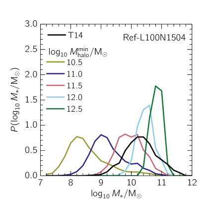
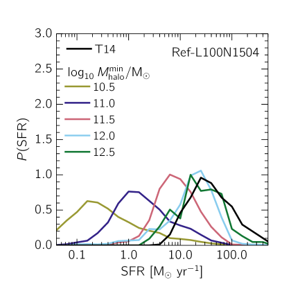
Figure 1: PDFs of galaxy stellar masses (left panel) and SFRs (right panel) for the KBSS galaxies in T14 (black lines), as well as for different $M_{\rm halo}^{\rm min}$ in the Ref-L100N1504 simulation (coloured lines). Previous measurements of the observed galaxy halo masses (Trainor & Steidel, 2012; Rakic et al., 2013) estimate $M_{\rm halo}^{\rm min}$ to be between $10^{11.5}$ and $10^{12.0}$ M_⊙ (represented by the red and cyan lines, respectively). The observed stellar masses agree very well with the simulations for these halo masses, while the observed SFRs are systematically somewhat higher than those of EAGLE by a factor of $\approx 2$.

3.1 The galaxy sample

We present the median stellar masses ($M_{\ast}$) and median star formation rates (SFRs) for each $M_{\rm halo}^{\rm min}$ sample in Table 5. We note that these are the true values measured directly from the simulations, not from virtual observations. For the observed sample, the median stellar mass is $\log_{10}M_{\ast}/{\rm M}_{\odot}=10.2$ and the median SFR is $30$ M_⊙ yr^-1. In both the observations and simulations, a Chabrier (2003) initial mass function is assumed. Furlong et al. (2015a) found that observations of the evolution of the galaxy stellar mass function are reproduced remarkably well in EAGLE. However, they noted that the normalization of the specific SFR is 0.2–0.4 dex below observations at all lookback times.

To compare directly with our galaxy sample, in Fig. 1 we present probability distribution functions (PDFs) of the stellar masses and SFRs for different minimum halo masses taken from the Ref-L100N1504 simulation, as well as from the observations. We will focus on the range of $M_{\rm halo}^{\rm min}=10^{11.5}\text{--}10^{12.0}$ M_⊙, which corresponds to median halo masses of $10^{11.8}$–$10^{12.2}$ M_⊙ (see Table 3) and agrees with the halo masses of the KBSS (Trainor & Steidel, 2012; Rakic et al., 2013). For this minimum halo mass range, we find very good agreement with the observed stellar masses, while the SFRs from the observations are systematically higher than in EAGLE (consistent with the findings of Furlong et al. 2015a), although the medians only differ by a factor of $\approx 2$ for $M_{\rm halo}^{\rm min}=10^{12.0}$ M_⊙. We conclude that performing the galaxy selection by stellar mass or SFR instead of halo mass would not significantly alter our results.

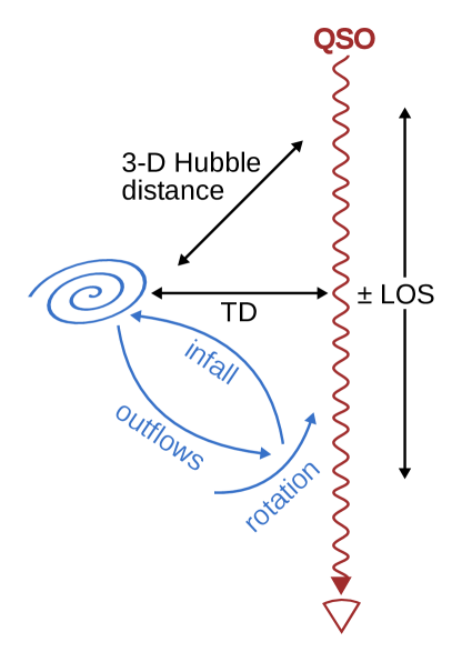
Figure 2: A schematic outlining the geometry of the observations. The blue spiral represents a galaxy, which has associated inflowing, outflowing and rotating gas, which is probed by the QSO sightline. The black lines denote the transverse distance (TD), LOS distance, and 3-D Hubble distance.

3.2 Synthesis of galaxy and quasar data

The large number of galaxies in the KBSS has provided a unique opportunity to analyze the absorption along the quasar LOS in a statistical fashion. To outline the geometry required to do so, we present a schematic of a galaxy next to a quasar sightline in Fig. 2. Note that the observational sample from T14 has 854 of such galaxies.

The galaxy is denoted by a blue spiral, and its redshift allows us to associate it with a specific region along the QSO sightline. The gas from the galaxy, which could be static, infalling, outflowing or rotating, is probed by the light from the background quasar. The velocity component of the gas tangent to the sightline will result in velocity- or redshift-space anisotropies in the absorption.

The black lines mark some quantities frequently presented in T14 and this work. The impact parameter or transverse distance (TD) is the projected distance between the galaxy and the sightline. The LOS distance, which also measures redshift and velocity, runs along the QSO sightline. Finally, the 3-D Hubble distance is simply the 3-D distance assuming pure Hubble flow.

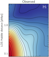
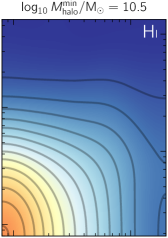
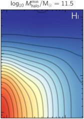
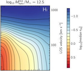
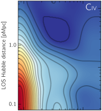
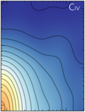
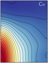
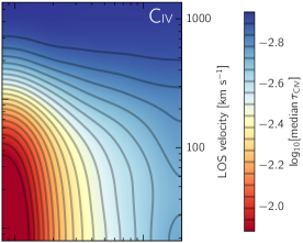
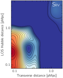
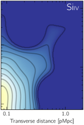
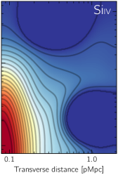
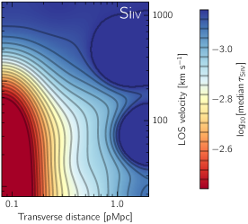
Figure 3: 2-D maps of median metal-line optical depth around galaxies, for Hi (top row), Civ (centre row) and Siiv (bottom row). The leftmost column shows the KBSS observations from T14, while the following three columns display the results from the Ref-L100N1504 EAGLE simulations, with an increasing minimum halo mass of $M_{\rm halo}^{\rm min}=10^{10.5}$, $10^{11.5}$, and $10^{12.5}$ M_⊙ from left to right. The observations have been smoothed with a Gaussian that has a $\sigma$ equal to the bin size (0.15 dex). The minimum optical depth values used in the colour scale are set to the median optical depth for random regions, which for each ion is by construction identical for the simulations and observations, while the maximum optical depth values are set by the maxima in the observations. The $p$-values, i.e. the probability that a model (with a given $M_{\rm halo}^{\rm min}$) is consistent with the observed unsmoothed data, are given in Table 6.

Table 6: $p$-values (i.e. the probability that a model, with a given $M_{\rm halo}^{\rm min}$, is consistent with the observed unsmoothed data) from Fig. 3. We measure $p$-values using data from the full maps, and for the case of Hi also for the same subset of bins used to measure halo mass as in Rakic et al. (2013). The data rule out all models with $M_{\rm halo}^{\rm min}\geq 10^{12.0}$ M_⊙, while all but the full map of Civ rule out $M_{\rm halo}^{\rm min}=10^{10.5}$ M_⊙.

$\log_{10}M_{\rm halo}^{\rm min}/{\rm M}_{\odot}$	$10.5$	$11.0$	$11.5$	$12.0$	$12.5$
Hi, full map	$0.002$	$0.059$	$0.033$	$0.000$	$0.000$
Hi, $\text{LOS}=0.71\text{--}2.83$ pMpc	$0.003$	$0.085$	$0.340$	$0.034$	$0.000$
Civ, full map	$0.063$	$0.410$	$0.326$	$0.012$	$0.000$
Siiv, full map	$0.001$	$0.000$	$0.049$	$0.011$	$0.000$

3.3 2-D optical depth maps

The primary results of T14 can be summarized by their Fig. 4, where they presented the first 2-dimensional (2-D) maps of metal-line absorption around galaxies. These maps were constructed by using the galaxy redshifts to associate each galaxy with a wavelength region in the QSO spectrum, as illustrated in Fig. 2. The recovered pixel optical depths for every galaxy were then binned by the TD and LOS distance to the galaxy, and the maps were made by taking the median pixel optical depth in each bin.

We reproduce the T14 maps of the median observed Hi, Civ and Siiv optical depths in the leftmost column of Fig. 3. T14 noted the presence of a strong enhancement of the absorption near galaxies with respect to random regions that extends $\sim 180$ pkpc in the transverse direction and $\sim\pm 240$ km s^-1 along the LOS. A second result was the detection of weak excess absorption out to a transverse distance of 2 pMpc, the maximum impact parameter probed, for Hi and Civ.

The observations are compared with simulated samples with minimum halo masses of $10^{10.5}$, $10^{11.5}$, and $10^{12.5}$ M_⊙, shown respectively in columns 2–4 of Figure 3. Although we will explore the comparison more quantitatively in the subsequent figures, we can already infer some characteristic behaviours from the 2-D maps. Primarily, we find that the strength of absorption, characterized by the pixel optical depths, by metals and Hi in the vicinity of galaxies increases with halo mass (from left to right), and that the effect is stronger for the metals. For Civ and Siiv, it appears that the $M_{\rm halo}^{\rm min}=10^{11.0}$ M_⊙ model produces too little absorption while the $M_{\rm halo}^{\rm min}=10^{12.0}$ M_⊙ produces too much, which suggests that the data agree most closely with a mass that lies within this range.

We would like to assess the goodness-of-fit of each of the models, however the $\chi^{2}$ statistic cannot be used because the errors are correlated and non-Gaussian. Instead, we compute $p$-values for each $M_{\rm halo}^{\rm min}$ considered here in the following manner. For a given realization of the simulated data, we use 10,000 bootstrap realizations of the observations (performed by bootstrapping the galaxies in each transverse bin) and determine, for each bin in the transverse and/or LOS direction, the percentile of the bootstrap realization that agrees with the simulations, where the percentiles are normalized to range from 0 to 50 (that is, if a percentile was $>50$, it was subtracted from $100$). Then, the percentiles corresponding to each LOS-impact parameter bin are divided by 100 and multiplied together to give a probability of the model. This procedure is also applied to all of the bootstrap realizations of the data, so that each realization has an associated probability. The $p$-values which we quote here are then given by the fraction of the realizations of the data that have a probability lower than that of the model. We note that if we pretend that the observations are the model, then this procedure yields $p$-values $\geqq 0.988$. We reject models with $p$-values $<0.05$.

In Table 6, we present the $p$-values for each $M_{\rm halo}^{\rm min}$, for both the full (unsmoothed) map shown in Fig 3 as well as for distances along the LOS limited to the four bins within 170–670 km s^-1 (or 0.71–2.83 pMpc for pure Hubble flow), as these bins were used in Rakic et al. (2013) to measure the halo mass from the Hi data. Rakic et al. (2013) chose this velocity range because there they found the Hi absorption to be insensitive to variations in subgrid physics models. For Hi, only the $M_{\rm halo}^{\rm min}=10^{11.0}$ M_⊙ model is consistent with the full map, but the $p$-value for $10^{11.5}$ M_⊙  (0.033) is less than a a factor of two smaller than for $M_{\rm halo}^{\rm min}=10^{11.0}$ (0.059). However, when using the restricted bin range of Rakic et al. (2013), the $M_{\rm halo}^{\rm min}=10^{11.5}$ M_⊙ model is accepted with $p=0.34$, in good agreement with Rakic et al. (2013).

Fitting to the full range of data points or the subset from Rakic et al. (2013) may, however, not be the best approach for Siiv, because most of the map is dominated by noise, as we do not detect significant absorption beyond $\sim 500$ pkpc in the transverse direction. Indeed, we find that all models are formally ruled out by the data, although the disagreement is only marginal for $M_{\rm halo}^{\rm min}=10^{11.5}$ M_⊙ ($p=0.049$). On the other hand, Civ fares much better, likely because the absorption above $\tau_{C\textsc{iv}}^{\rm rnd}$ extends out to the full impact parameter range of 2 pMpc. For the full map, we find that models with $M_{\rm halo}^{\rm min}=10^{10.5}\text{--}10^{11.5}$ M_⊙ are consistent with the Civ observations.

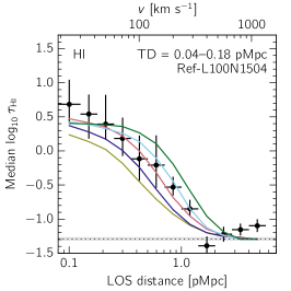
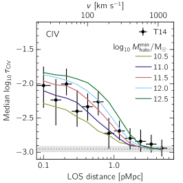
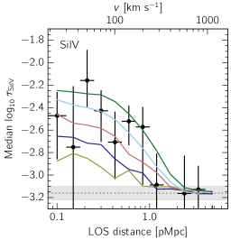
Figure 4: Cuts taken along the LOS through the maps from Fig. 3 (right column of Fig. 6 from T14). The upper horizontal axis indicates the velocity along the LOS, while the lower horizontal axis gives the corresponding physical distance assuming pure Hubble flow. The size of the transverse bin, 0.04–0.18 pMpc, was chosen to include the strong absorption in both Hi and metals. The observations from T14 are shown as black circles with 1-$\sigma$ error bars, while the simulations are denoted by the lines where each colour represents a different minimum halo mass. The horizontal dotted lines indicate $\tau_{Z}^{\rm rnd}$, and the grey region shows the 1-$\sigma$ scatter. The $p$-values for each halo mass model, based on the comparison shown here and on the cuts along the transverse direction shown in Fig. 5, are given in Table 7. Only the model with $\log_{10}M_{\rm halo}^{\rm min}/{\rm M}_{\odot}=11.5$ is consistent with all three ions.

3.4 Cuts along the LOS and transverse directions

To avoid comparing noise with noise, we confront the simulations with the regions of the 2-D maps that contain the most signal (Fig. 6 from T14). In Fig. 4 we show a cut that runs along the LOS, where the inner two impact parameter bins (ranging from 35 to 180 pkpc) were combined. From left to right, the panels show the median optical depth as a function of LOS distance for Hi, Civ and Siiv. Note that the y-axis range depends on the ion in question, and that the dynamic range is much larger for Hi than for the metal ions. The observations are shown with black circles, while the coloured curves show the simulation results for halo masses ranging from $10^{10.5}$ to $10^{12.5}$ M_⊙, in intervals of 0.5 dex.

Examining Hi in the left panel, we see that the Hi optical depths are most sensitive to halo mass at intermediate velocities ($v\approx 100$–$200$ km s^-1). For all minimum halo masses considered, the optical depths appear to be systematically lower than the $\sim 2$ innermost measurements (out to 40 km s^-1). However, we emphasize that the errors along the LOS are correlated (to scales of $\sim 10^{2}$ km s^-1, see Rakic et al. 2012) and that the observations and model agree at the 1-$\sigma$ level for all but the lowest halo masses, so this apparent discrepancy is not significant.

Turning next to the metals, we find that in contrast to Hi, the median optical depths within 60 km s^-1 of the galaxy positions are sensitive to halo mass. This halo mass dependence continues up to $\sim 600$ km s^-1 where all curves asymptote to $\tau_{Z}^{\rm rnd}$. Overall, we find that all the minimum halo masses considered here are consistent with the qualitative behaviour of the observations, which is that the metal-line absorption is strongly enhanced with respect to $\tau_{Z}^{\rm rnd}$ out to $\sim\pm 200$ km s^-1 along the LOS.

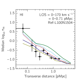
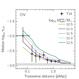
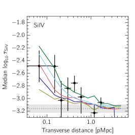
Figure 5: The same as Fig. 4, except taking a cut along the transverse direction of Fig. 3 with a width $\Delta v=\pm 170$ km s^-1 of the LOS (left-hand column of Fig. 6 in T14) The enhancement of Hi and Civ absorption out to the maximum observed impact parameter of 2 pMpc is also seen in the simulations, where it extends out to $\sim 5$ pMpc. The $p$-values resulting from a simultaneous comparison to this data plus that in Fig. 4 are given in Table 7.

Table 7: $p$-values for the models given the data shown in Figs. 4 and 5. Only the model with $M_{\rm halo}^{\rm min}=10^{11.5}$ M_⊙ is consistent with all the data.

$\log_{10}M_{\rm halo}^{\rm min}/{\rm M}_{\odot}$	$10.5$	$11.0$	$11.5$	$12.0$	$12.5$
Hi	$0.003$	$0.055$	$0.133$	$0.010$	$0.000$
Civ	$0.379$	$0.926$	$0.938$	$0.285$	$0.003$
Siiv	$0.023$	$0.035$	$0.099$	$0.068$	$0.030$

In Fig. 5 we examine cuts along the transverse direction, with a velocity width of $\pm 170$ km s^-1. This velocity cut was chosen because it corresponds to the scale on which $\tau_{\rm H\textsc{i}}$ is smooth, and because it is larger than the correlation scale (Rakic et al., 2011).

The simulations again capture the qualitative behaviour of the observations. The enhancement in the absorption decreases with the impact parameter and this gradient decreases with the distance from the galaxy. For all halo masses considered, the Hi and Civ median optical depths show enhancement above $\tau_{Z}^{\rm rnd}$ out to $\approx 5$ pMpc in EAGLE. T14 postulated that the significant excess absorption extending out to the maximum impact parameter of 2 pMpc in the observations (i.e., many virial radii away from the host galaxy) is likely due to clustering effects. Support for this argument is given by Fig. 8, which shows that the median optical depths are not fully converged for box sizes $<50$ cMpc, where clustering on $\sim$Mpc scales is not properly captured.

Finally, in Table 7 we present the $p$-values of simultaneous comparisons to the data from Figs. 4 and 5. The Hi data are consistent with $M_{\rm halo}^{\rm min}$ between $10^{11.0}$ and $10^{11.5}$ M_⊙. While the Civ data only exclude the highest minimum halo mass model, $10^{12.5}$ M_⊙, the Siiv data are consistent with $M_{\rm halo}^{\rm min}=10^{11.5}\text{--}10^{12.0}$ M_⊙. Therefore, only the model with $M_{\rm halo}^{\rm min}=10^{11.5}$ is consistent with all of the data.

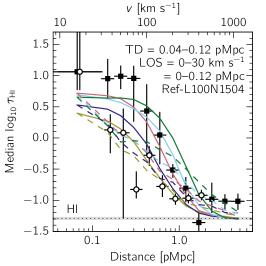
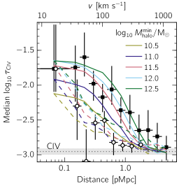
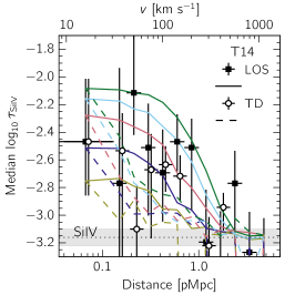
Figure 6: The median optical depth from cuts of equal size taken in the transverse direction (0.04–0.12 pMpc) and along the LOS ($\Delta v=\pm 30$ km s^-1, equivalent to 0.12 pMpc assuming pure Hubble flow), in order to study the redshift-space distortions (Fig. 5 in T14). The observed medians and 1-$\sigma$ errors are indicated in black, while the coloured lines show simulations using different $M_{\rm halo}^{\rm min}$. The filled squares and solid lines denote the median optical depths along the line-of-sight, denoted LOS, while the open circles and dashed lines indicate the transverse direction, denoted TD. The $p$-values for the models are given in Table 8.

Table 8: $p$-values for the models given the data shown in Fig. 6. While the Hi data rule out all minimum halo masses except for $M_{\rm halo}^{\rm min}=10^{11.5}$ M_⊙, the metal-line absorption data are less constraining.

$\log_{10}M_{\rm halo}^{\rm min}/{\rm M}_{\odot}$	$10.5$	$11.0$	$11.5$	$12.0$	$12.5$
Hi	$0.003$	$0.026$	$0.109$	$0.027$	$0.000$
Civ	$0.100$	$0.484$	$0.835$	$0.474$	$0.074$
Siiv	$0.219$	$0.040$	$0.316$	$0.229$	$0.143$

3.5 Redshift-space distortions

In Fig. 6 we examine redshift-space distortions, i.e., how the absorption along the LOS differs from that of the transverse direction (Fig. 5 from T14). We have plotted the median optical depths from the innermost bin (TD=0.04–0.13 pMpc, $\Delta v=\pm 30$ km s^-1) along the LOS (solid lines, filled squares for the observations) and the transverse direction (dashed lines, open circles for the observations). Note that along the LOS, this bin spans a total of 60 km s^-1, so its size is not significantly smaller than the magnitude of most redshift errors.

Fig. 6 demonstrates that the data and models show strong and comparable redshift-space distortions. The $p$-values for the comparisons are given in Table 8. The Hi data rule out all models except for $M_{\rm halo}^{\rm min}=10^{11.5}$ M_⊙, but the metal data do not provide strong constraints on the model halo mass. Although a simple “chi-by-eye” would eliminate the lowest-mass models, we reiterate that the errors are non-Gaussian and that along the LOS they are correlated.

The results for Hi in Fig. 6 can be directly contrasted with the top left panels of Fig. 7 (for points along the LOS) and Fig. 8 (for points in the transverse direction) in Rakic et al. (2013). In these figures, the authors examined the same optical depth profiles from the KBSS observations as are shown here, but using an older set of KBSS measurements with larger redshift errors, and compared the results to the OWLS simulations. They found that in the smallest transverse distance bin, the OWLS simulations significantly underestimated the highest observed Hi optical depths. The relative success of the EAGLE simulations compared to those presented in Rakic et al. (2013) can be partly attributed to the smaller redshift errors in the latest KBSS data, however even after removing redshift errors the Hi optical depths in Rakic et al. (2013) were still well below those from the observations. We conclude that the EAGLE simulations provide much better agreement to observations of Hi in absorption than was found for OWLS.

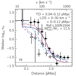
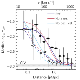
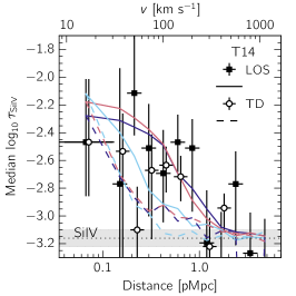
Figure 7: The same as Fig. 6, but only presenting $M_{\rm halo}^{\rm min}=10^{11.5}$ M_⊙, and comparing to models without redshift errors (red line) and without peculiar velocities (cyan line). Without redshift errors, the median optical depths decrease more steeply along the LOS, and there is also more absorption along the transverse direction for the velocity bin shown (0–30 km s^-1). Without peculiar velocities, the median optical depths along the LOS and transverse directions are almost identical, with the former still being slightly smoothed by the redshift errors. Thus, peculiar velocities are required to obtain the large observed redshift space distortions.

Table 9: $p$-values for the models given the data shown in Fig. 7. In this case, rather than computing the likelihood of the individual pixel optical depth values of a model given the data, we compute the likelihood of the difference between the LOS and TD optical depths, i.e. the magnitude of the anisotropy. We find that models in which peculiar velocities have been turned off are ruled out by the Hi and Civ data.

	Hi			Civ			Siiv
$\log_{10}M_{\rm halo}^{\rm min}/{\rm M}_{\odot}$	$11.0$	$11.5$	$12.0$	$11.0$	$11.5$	$12.0$	$11.0$	$11.5$	$12.0$
Ref	$0.022$	$0.117$	$0.182$	$0.147$	$0.352$	$0.392$	$0.033$	$0.389$	$0.180$
No z err.	$0.005$	$0.037$	$0.092$	$0.063$	$0.223$	$0.333$	$0.033$	$0.433$	$0.214$
No pec. vel.	$0.021$	$0.034$	$0.043$	$0.038$	$0.046$	$0.040$	$0.040$	$0.576$	$0.246$

4 Origin of redshift-space distortions

In this section we will exploit the simulations to probe the origin of the observed redshift-space distortions, which may be caused by gas inflows, outflows, virial motions, or galaxy redshift errors. We begin by attempting to disentangle the effects of redshift errors from gas peculiar velocities. In Fig. 7, we show the same redshift-space distortions as in Fig. 6, but we have now added a simulation without any redshift errors. As demonstrated previously in Rakic et al. (2013, see also Tummuangpak et al. 2014) we find that the removal of redshift errors increases the median optical depths at small galactocentric distances, both in the transverse direction and along the LOS. However, the effect is modest because the KBSS redshift errors are small for most galaxies (see § 2.2). Thus, it is likely that the elongation along the LOS is mostly due to differences between the peculiar velocities of the galaxy and the absorbing gas.

To test this, we have run SPECWIZARD with galaxy and gas peculiar velocities set to zero, and plot the result as the cyan lines in Fig. 7. The redshift-space distortions for the cyan lines are strongly suppressed compared to the other cases, i.e., the solid and dashed lines are much closer together, with the remaining difference due to redshift errors. Turning off peculiar velocities decreases the median optical depths along the LOS, except for the innermost bin. We note that if we exclude redshift errors and turn off peculiar velocities simultaneously, the optical depths along the LOS and in the transverse direction are nearly identical.

We know from the previous section that the models with $M_{\rm halo}^{\rm min}=10^{11.5}$ are not ruled out by the data. To check whether in the absence of redshift errors or peculiar velocities the predicted redshift space distortions are consistent with the observations, instead of computing the $p$-values using the individual pixel optical depth values, we use the difference in optical depths between the LOS and transverse directions, i.e. the magnitude of the anisotropy. The results of this calculation are presented in Table 9. While the data do not fully rule out the models without redshift errors, for Hi and Civ we find that the models without peculiar velocities do not produce redshift-space anisotropies consistent with the data. We note that the Siiv data, which are much noisier than Hi and Siiv, are inconclusive on this point. Overall, the simulations provide strong evidence that the redshift-space distortions arise due to the motion of the gas, rather than galaxy redshift errors.

Next, we can employ the simulations to explore the net direction of the gas velocity, i.e. whether we are probing infalling, outflowing or rotating gas. T14 measured a strong enhancement of the optical depths along the LOS to about $\pm 240$ km s^-1, which is close to the galaxies’ circular velocities ($\approx 217$ km s^-1). Thus, it was not previously possible to differentiate between the virial motion and outflow scenario. Other observations also do not offer conclusive evidence. On the one hand, Steidel et al. (2010) found ubiquitous outflows by using the KBSS galaxies as background sources to probe their own gas in absorption. On the other hand, large scale infall of Hi has been observed not just around galaxies in the KBSS (Rakic et al., 2012) but in other samples of Lyman break galaxies (e.g., Bielby et al., 2016). Indeed, simulations by Kawata & Rauch (2007) found that symmetric absorption features around a galaxy were produced by filamentary accretion.

In Fig. LABEL:fig:velocity, we present the gas particle radial velocities as a function of radial distance from galaxy centres. To calculate the velocities, we consider all galaxies in the simulation box above a specific mass threshold, and for each of these galaxies we calculate the radial velocity of each gas particle relative to its centre of mass. The median velocities are then weighted by, from left to right in Fig. LABEL:fig:velocity, mass, volume, and ion mass for Hi, Civ, and Siiv, respectively. We note that ion masses are calculated using the same interpolation tables that were used to generate the mock spectra.

While we have plotted the mass- and volume-weighted median gas velocities to get a picture of the behaviour of the total gas content, in order to use the results from Fig. LABEL:fig:velocity to interpret the observed redshift-space distortions, we argue that the ion mass-weighted quantities provide the most appropriate comparison. Along a single sightline that intersects various gas clouds, the pixels will be ion column density-weighted, given by the ion density multiplied by the kernel. However, a group of sightlines is also cloud cross section-weighted, since larger gas clouds are more likely to be intercepted. This effect contributes a kernel² term to the weighting, and taken together, the product of the ion density and kernel³ results in the ion mass.

In the top row of Fig. LABEL:fig:velocity, we show results for all galaxies with a minimum halo mass of $10^{11.5}$ M_⊙, while in the bottom row we use a minimum fixed stellar mass of $10^{9.5}$ M_⊙, and in each case we not only consider the reference model, but also the strong and weak feedback models (hence, the smaller L025N0376 box was used). We do so because we would like to know how the gas velocities vary with stellar mass at fixed halo mass, and vice versa. Table 5 demonstrates that for a fixed minimum halo mass, the StrongFB (WeakFB) model produces galaxies with smaller (larger) stellar masses than the reference model. It follows that at a fixed minimum stellar mass, the StrongFB (WeakFB) model galaxies reside in more (less) massive halos. Specifically for $\log_{10}M_{\ast}^{\rm min}/{\rm M}_{\odot}=9.5$, we find median $\log_{10}M_{\rm halo}/{\rm M}_{\odot}=(11.5,11.7,12.1)$ for WeakFB, Ref, and StrongFB, respectively

The first point to note in Fig. LABEL:fig:velocity is that the ion mass-weighted gas particle velocities, including the 1-$\sigma$ scatter, are mostly negative, which indicates that the net direction of the gas probed by these ions is typically towards the host galaxy (infalling). In contrast, the mass- and volume-weighted velocities are more positive, and in the latter case are mostly outflowing at the smallest radial distances. The volume-weighted velocities are most sensitive to outflows because outflows tend to be hot and diffuse with high volume-filling factors.

Next, focusing on the ion mass-weighted velocities in the top row, where we have used a fixed minimum halo mass, we find that varying the feedback model (and hence the stellar mass) has almost no effect on the gas velocities. Furthermore, in the bottom row where we have used a fixed minimum stellar mass, the gas velocities do depend on the feedback model. In particular, at fixed stellar mass the velocities decrease (become more infalling) with increasing feedback strength (and thus increasing halo mass). Since the galaxy gas accretion velocity is expected to increase with halo mass, in addition to the fact that we are seeing primarily negative velocities, this suggests that Hi, Civ and Siiv primarily trace infalling gas.

Since outflows are thought to be driven by energetic feedback from star formation and AGN, if the observed redshift-space distortions were dominated by outflowing gas, one would expect a significant difference between models with substantially different feedback physics. In Appendix C, we study how the optical depth profiles are affected by varying the feedback model, and we find only modest differences in the metal-line absorption properties. This supports the above finding, that the observed redshift-space anisotropies are dominated by virial motions and/or inflows, rather than by outflowing gas.

5 Discussion and conclusions

We have compared the circumgalactic Hi and metal-line absorption in the EAGLE cosmological hydrodynamical simulations with observations. EAGLE includes subgrid prescriptions for stellar and AGN feedback that have been calibrated to match observations of the $z\sim 0$ galaxy stellar mass function, the black hole-galaxy mass relation, and galaxy disk sizes. The fiducial EAGLE model has been run with a relatively high resolution ($\epsilon\sim 1$ pkpc at $z\approx 2$) in a cosmologically representative box size (100 cMpc).

In this work we compare the results from EAGLE to observations from T14. T14 used data from the KBSS, a spectroscopic galaxy survey in 15 QSO fields, to study the properties of the gas around 854 star-forming galaxies at $z\approx 2$. They applied the pixel optical depth technique to the QSO spectra and combined the absorption information with the positions and redshifts of the galaxies in the field to construct the first 2-D maps of metal-line absorption around galaxies.

We have used the simulations to generate mock spectra that were designed to mimic the properties of the QSO spectra from the KBSS. The galaxy impact parameter distribution and redshift errors were also matched to those of the observations. We compared the simulated and observed optical depths of Hi, Civ and Siiv as a function of transverse and LOS separation from galaxies. Our main conclusions are:

• The galaxy stellar masses from EAGLE are in very good agreement with the observations for $M_{\rm halo}^{\rm min}=10^{11.5}$–$10^{12.0}$ M_⊙(corresponding to median halo masses of $10^{11.8}$–$10^{12.2}$), which is the halo mass range inferred from observations (Trainor & Steidel, 2012; Rakic et al., 2013). The SFRs also show broad agreement, especially for $M_{\rm halo}^{\rm min}=10^{12.0}$, which matches the observed SFR PDF closely and has a median SFR only a factor of two below that of the observations (Fig. 1).

• The EAGLE simulations reproduce the observed Hi, Civ and Siiv absorption around galaxies in detail, including the redshift-space distortions. The observations are most consistent with a minimum halo mass of $10^{11.5}$ M_⊙, in agreement with Rakic et al. (2013) (Figs. 3, 4, 5).

• T14 detected enhanced median optical depths for Hi and Civ in the transverse direction out to impact parameters of 2 physical Mpc (pMpc); the maximum in their sample). The simulations are consistent with this result, and predict that this enhancement extends to $\approx 5$ pMpc (Fig. 5). This large-scale enhancement is not seen in the 25 cMpc simulation box, and we conclude that it is due to clustering (Fig. 8).

• Although redshift errors smooth optical depths along the LOS and reduce them slightly in the transverse direction, the very small redshift errors for galaxies observed with MOSFIRE ($\approx 18$ km s^-1) have a negligible effect on the results (Fig. 7).

• Gas peculiar velocities generate the significantly higher median optical depths along the LOS compared to the transverse direction (Fig. 7).

• The median ion mass-weighted radial gas velocities indicate that the bulk of the absorbing gas is flowing inward towards the galaxies, and that inflow rates increase with halo mass, but are insensitive to the strength of feedback at fixed halo mass (Fig. LABEL:fig:velocity). We also find that the optical depths do not change significantly when the stellar feedback strength is varied by a factor of two (Fig. 11), or when AGN feedback is neglected (Fig. 12). It is therefore likely that the observed enhancement of optical depths along the LOS compared to the transverse direction is not caused by outflows, but rather by infalling gas.

The results from this work are seemingly in tension with those of Steidel et al. (2010), who used the same sample of galaxies as background sources to probe their own gas in absorption , and measured ubiquitous outflows in Civ and Siiv. It is plausible that this discrepancy is due to geometrical effects, for example such “down-the-barrel” observations may be sensitive to the gas at much smaller galactocentric distances. As a caveat we mention that our conclusion that the gas is accreting is based entirely on the comparison with simulations.

It is also informative to compare these findings with those of Turner et al. (2015), who used the same KBSS dataset and found that at small galactocentric distances, Ovi traces hot, collisionally ionized, outflowing gas, in contrast to what we see in this study for Civ and Siiv. However, Ovi has a higher ionization potential than Civ and Siiv. Furthermore, Turner et al. (2015) found that the hot outflowing material can only be identified when there is no chance superposition of pixels with high Hi optical depths, while conversely, in this work we are considering all pixels close to galaxies. Taken together, the results from Turner et al. (2015) and this work imply that the two distinct gas phases inhabit the same regions around galaxies, while having different kinematics. The hot phase may be significant, but it is much more difficult to detect.

As a next step, we would like to perform an analysis similar to Turner et al. (2015) using the simulations. However, Ovi is not as straightforward to analyze in the simulations as the ions studied in this work, as it is located in the Ly$\beta$ forest and therefore suffers from strong contamination from Hi Lyman series lines. This contamination must be modelled, which we leave for a future study.

Appendix A Resolution and box size tests

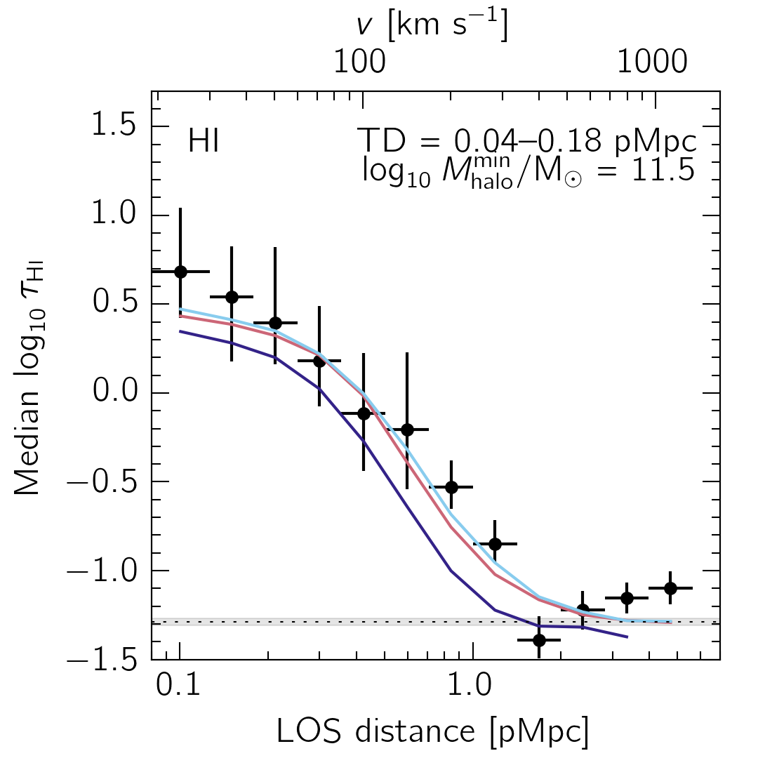
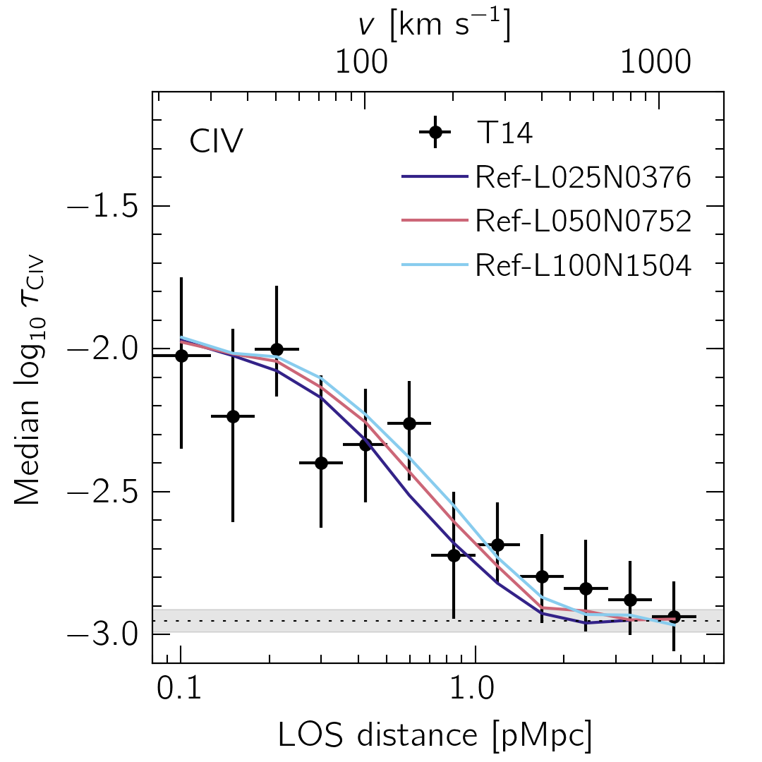
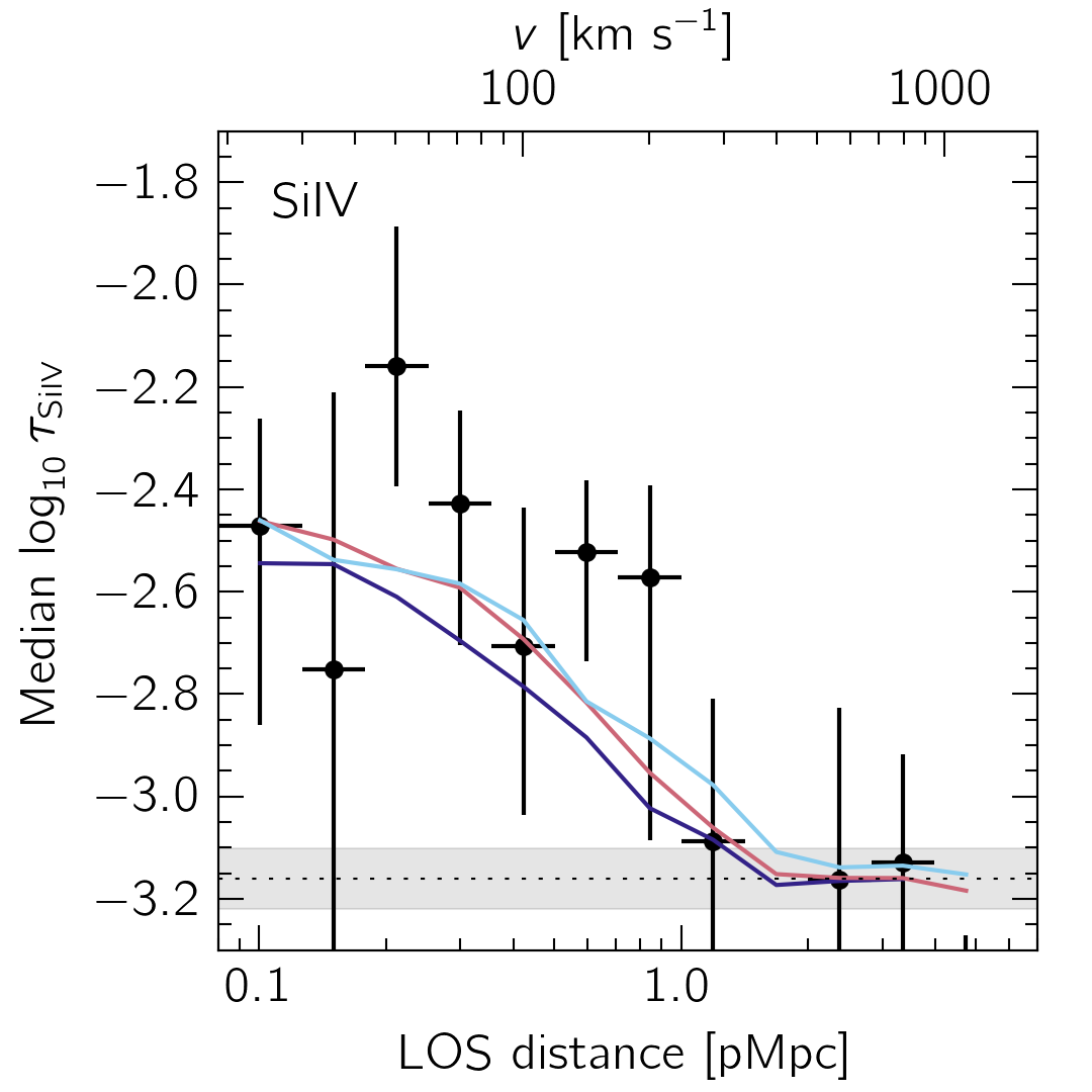
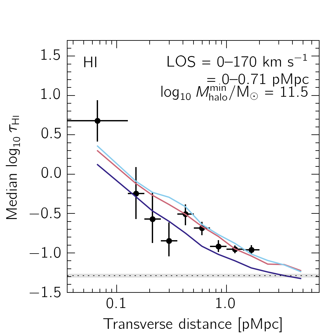
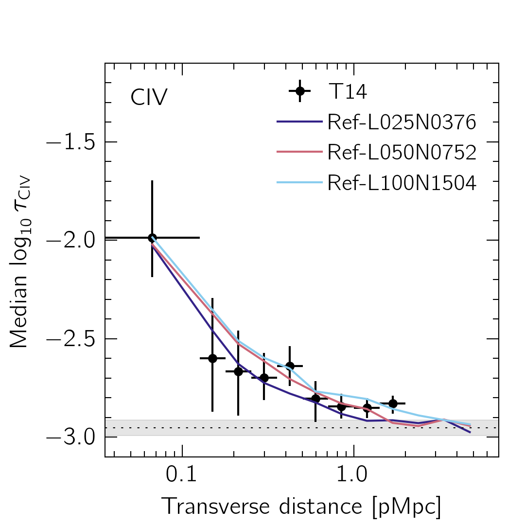
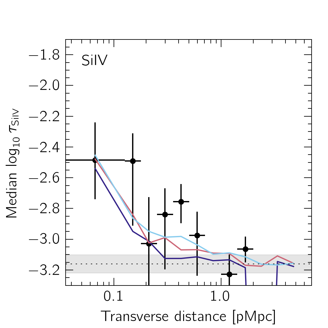
Figure 8: Convergence with respect to simulation box size, where we plot the median optical depths as a function of distance from galaxies along the LOS (top row) and in the transverse direction (bottom row). From left to right we show Hi, Civ, and Siiv for $M_{\rm halo}^{\rm min}=10^{11.5}$ M_⊙. While the optical depths from the 25 cMpc box are systematically lower than for the other runs, our fiducial simulation is converged.

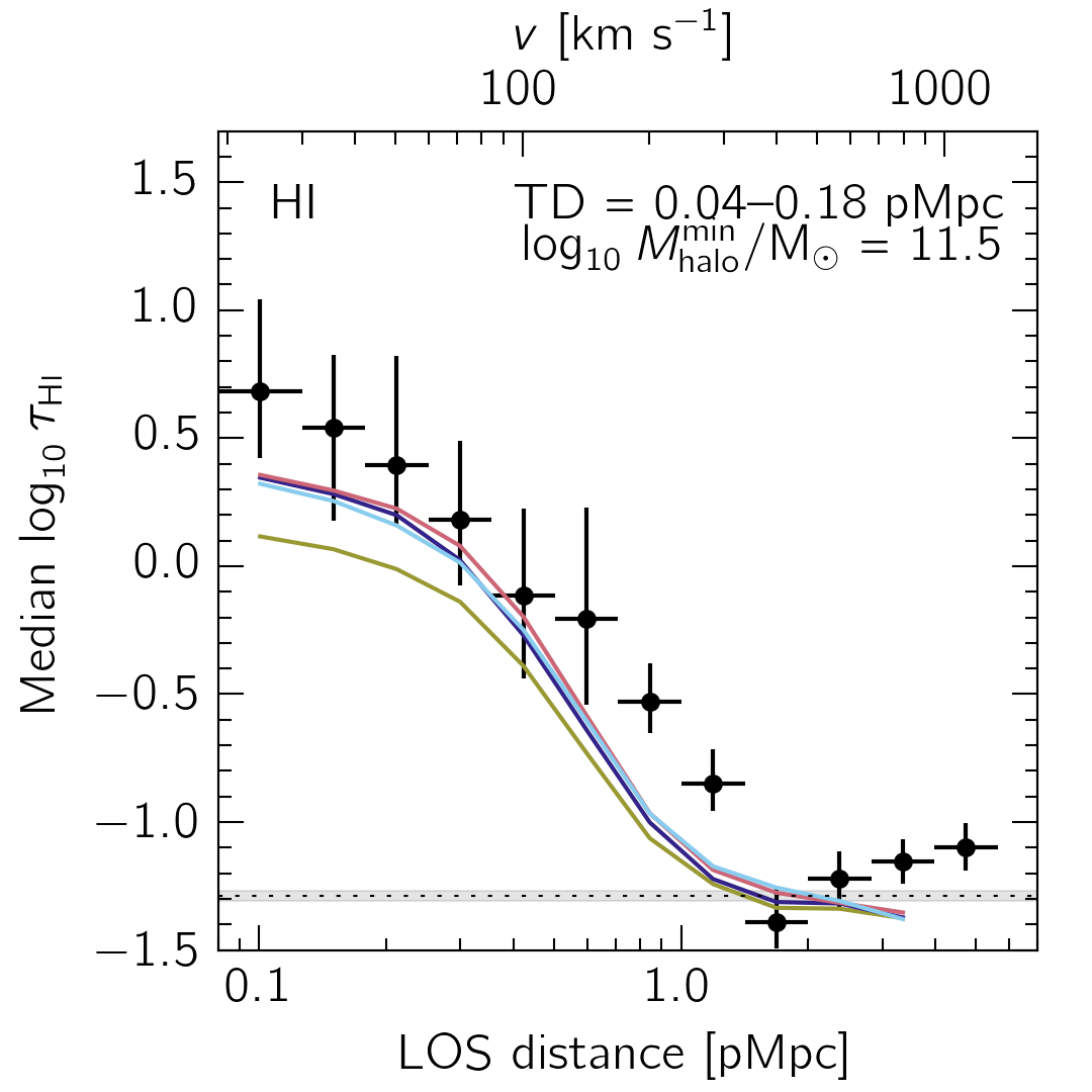
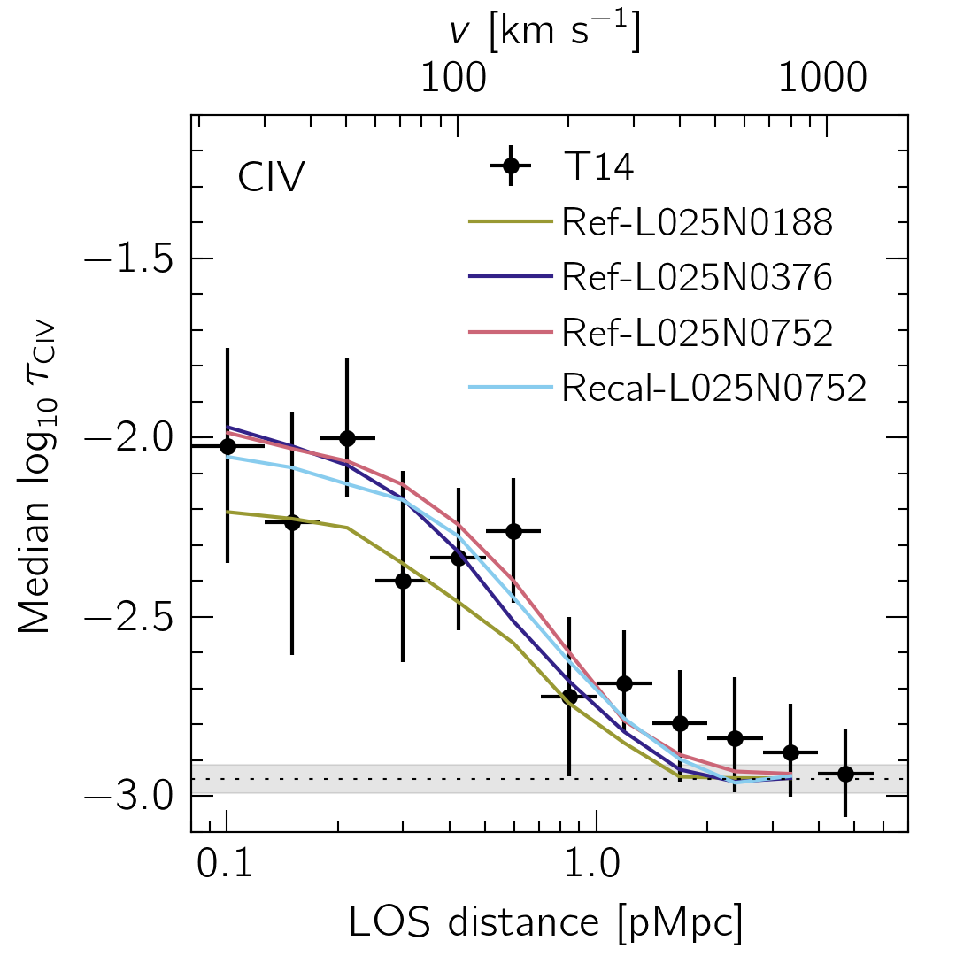
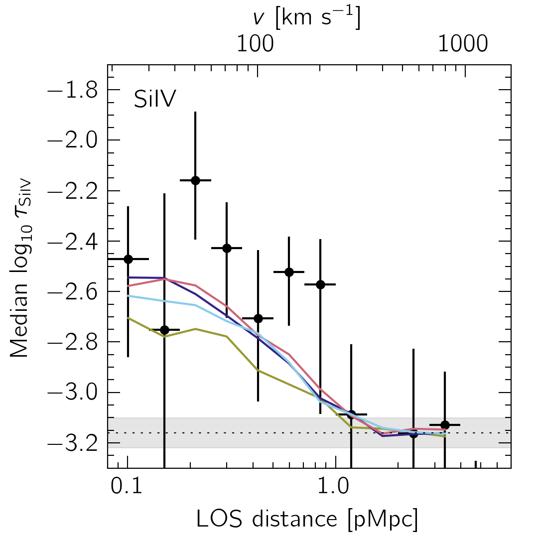
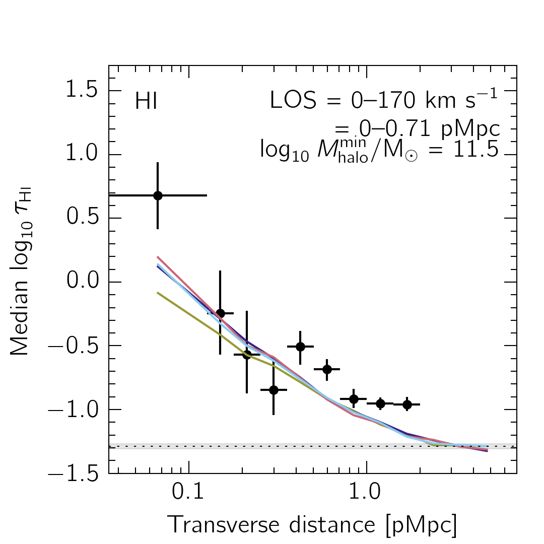
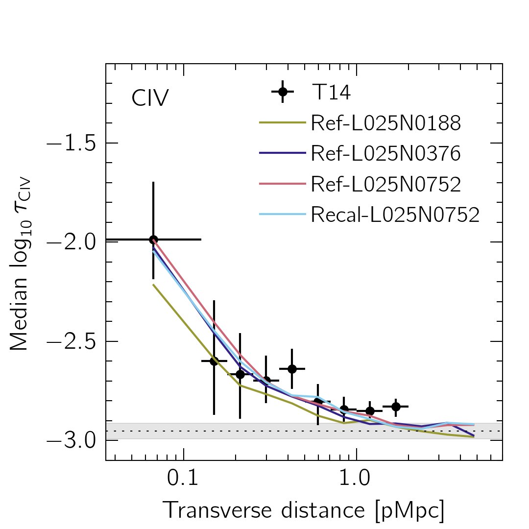
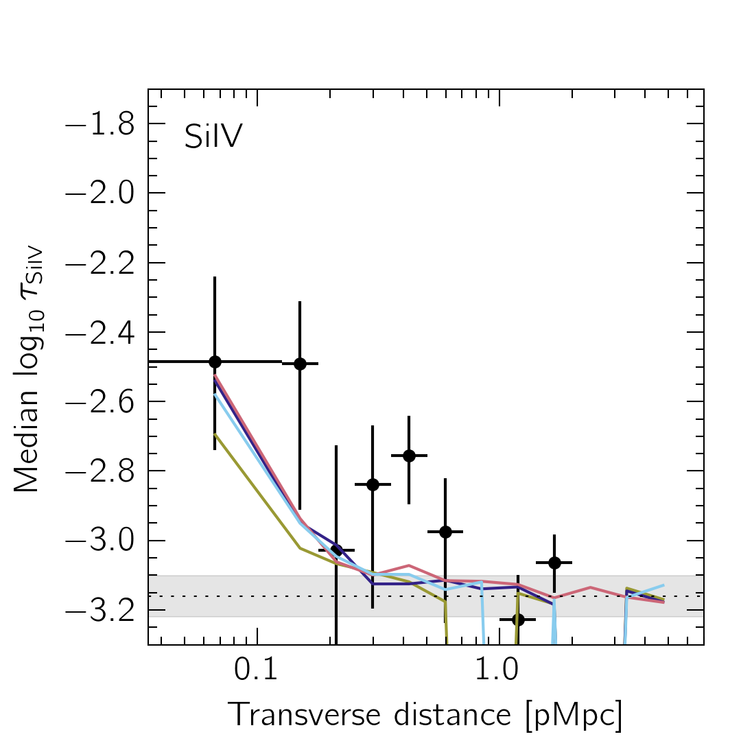
Figure 9: The same as Fig. 8, but instead presenting convergence with respect to the numerical resolution. We use the 25 cMpc box simulations showing the reference model for $188^{3}$, $376^{3}$ and $752^{3}$ particles, in addition to the recalibrated L025N0752 run. The lowest-resolution run, Ref-L025N0188, has lower median optical depths in the innermost LOS and transverse distance bins compared to realizations with higher resolutions,but the fiducial intermediate- and high- resolution runs agree, indicating that the fiducial simulation is converged.

We examine the effects of varying the simulation box size in Fig. 8, where we plot the same cuts along the LOS (top row) and transverse distance (bottom row) as were shown in Figs. 4 and 5. We show results from the fiducial model Ref-L100N1504, as well as from the reference run in the 50 and 25 cMpc boxes with the same resolution. The median optical depth profiles for the 50 and 100 cMpc runs are converged, while for the 25 cMpc box the optical depths tend to be lower, likely because the median halo masses are smaller in the 25 cMpc box (see Table 3).

To test the effects of varying resolution, we turn to the 25 cMpc box which has been realized with resolutions higher than the fiducial one used in this work. The L025N0752 simulation includes a version that has been run using the subgrid physics of the reference model (Ref-) and one that has been recalibrated to better match the $z\approx 0$ galaxy stellar mass function (Recal-). In Fig. 9 we plot the median optical depths along the LOS (top row) and transverse distance (bottom row) for these high-resolution runs as well as for our fiducial resolution ($376^{3}$ particles in the 25 cMpc box) and finally a lower resolution of $188^{3}$ particles.

We find that for all ions and halo masses, the optical depth profiles from the fiducial and high-resolution runs are in agreement, while those from the low-resolution runs are systematically lower. We can therefore conclude that our fiducial simulation is converged.

Appendix B Addition of minimum contamination level

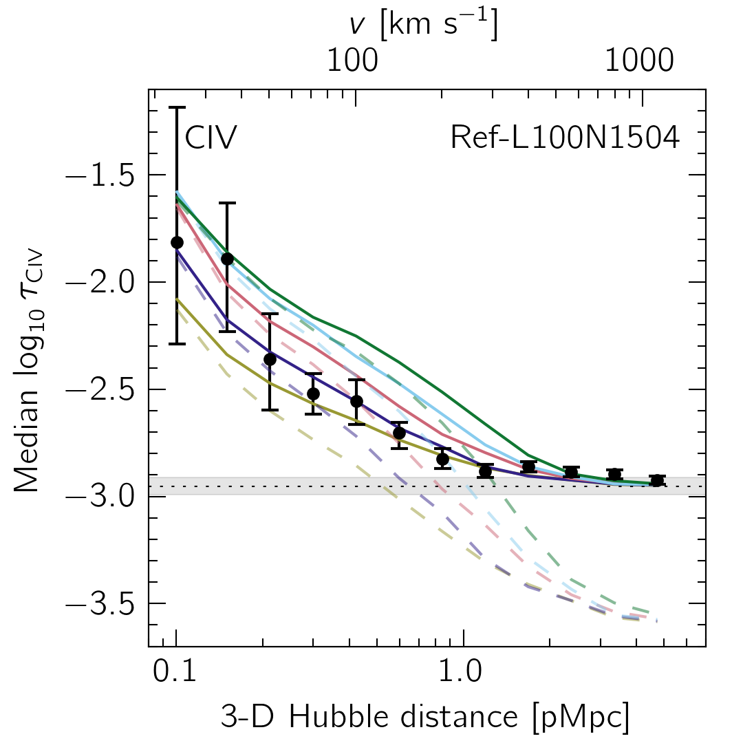
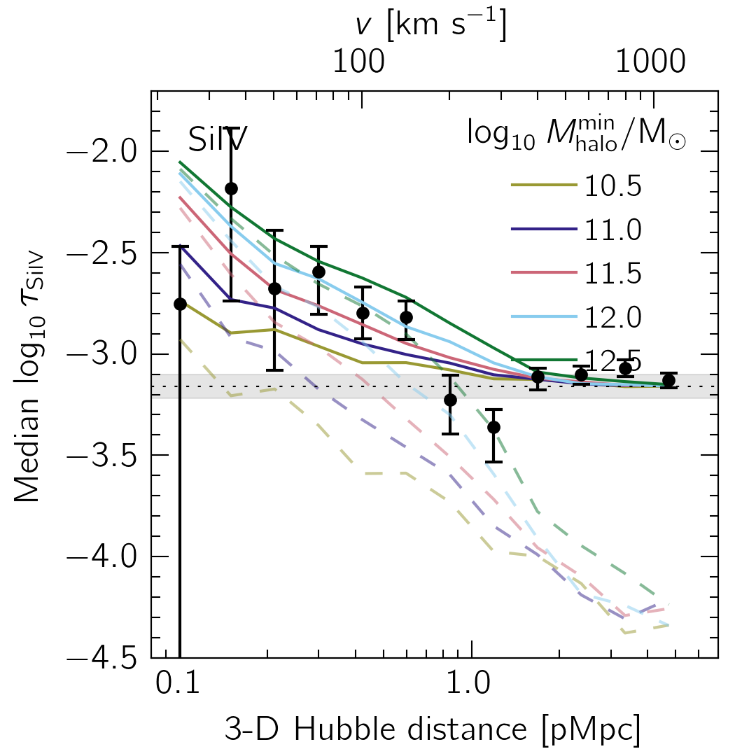
Figure 10: Median optical depths against 3-D Hubble distance, for Civ (left) and Siiv(right). As in previous figures, the filled black points denote the observations, while the simulations are represented by the lines. Here, the dashed (solid) lines show the optical depth profiles before (after) the addition of $\Delta\tau_{Z}^{\rm rnd}$. While equalizing $\tau_{Z}^{\rm rnd}$ between the observations and simulations is important for comparing the optical depths at larger distances, it does not substantially alter the well-detected signal in the innermost bins ($v\lesssim 100$ km s^-1).

In § 2, we describe how $\tau_{Z}^{\rm rnd}$, the median pixel optical depth in random regions, is lower in the simulations than in the observations, probably due to the absence of contamination in the mock spectra. For the figures in the main text, we simply add $\Delta\tau_{Z}^{\rm rnd}$, defined as the difference between simulated and observed $\tau_{Z}^{\rm rnd}$, to the simulated optical depths, primarily to facilitate comparison at larger galactocentric distances.

To quantify the impact of this procedure, in Fig. 10 we have plotted the median pixel optical depths for Civ and Siiv as a function of 3-D Hubble distance, defined as $\sqrt{b^{2}+\left(\Delta v/H\left(z\right)\right)^{2}}$, a metric that allows us to combine together both the transverse and LOS direction information. The dashed lines in Fig. 10 show the simulated median pixel optical depths before adding $\Delta\tau_{Z}^{\rm rnd}$, while the solid lines demonstrate the result of the addition.

The dashed lines demonstrate that the addition of $\Delta\tau_{Z}^{\rm rnd}$ does not significantly impact the innermost bins where the optical depths are detected with high confidence above $\tau_{Z}^{\rm rnd}$. This gives us assurance that the selected simulated galaxies are producing enough metals to reproduce the observations. Rather, the main impact of $\Delta\tau_{Z}^{\rm rnd}$ is on the slope of the optical depth profiles. With or without the addition of $\Delta\tau_{Z}^{\rm rnd}$, it is clear that the observed and simulated median optical depths exhibit the same qualitative behaviour, with values peaking in the innermost bins and decreasing with distance until they reach $\tau_{Z}^{\rm rnd}$.

Appendix C Variation of feedback models

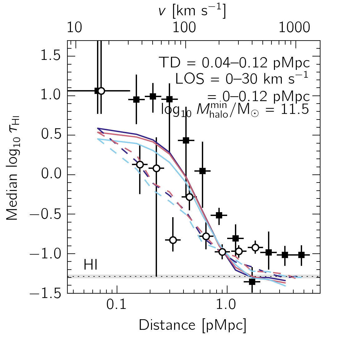
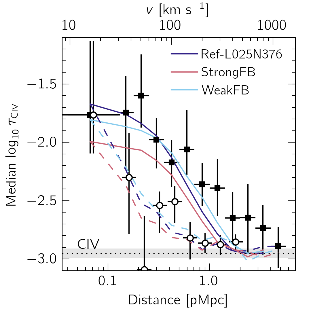
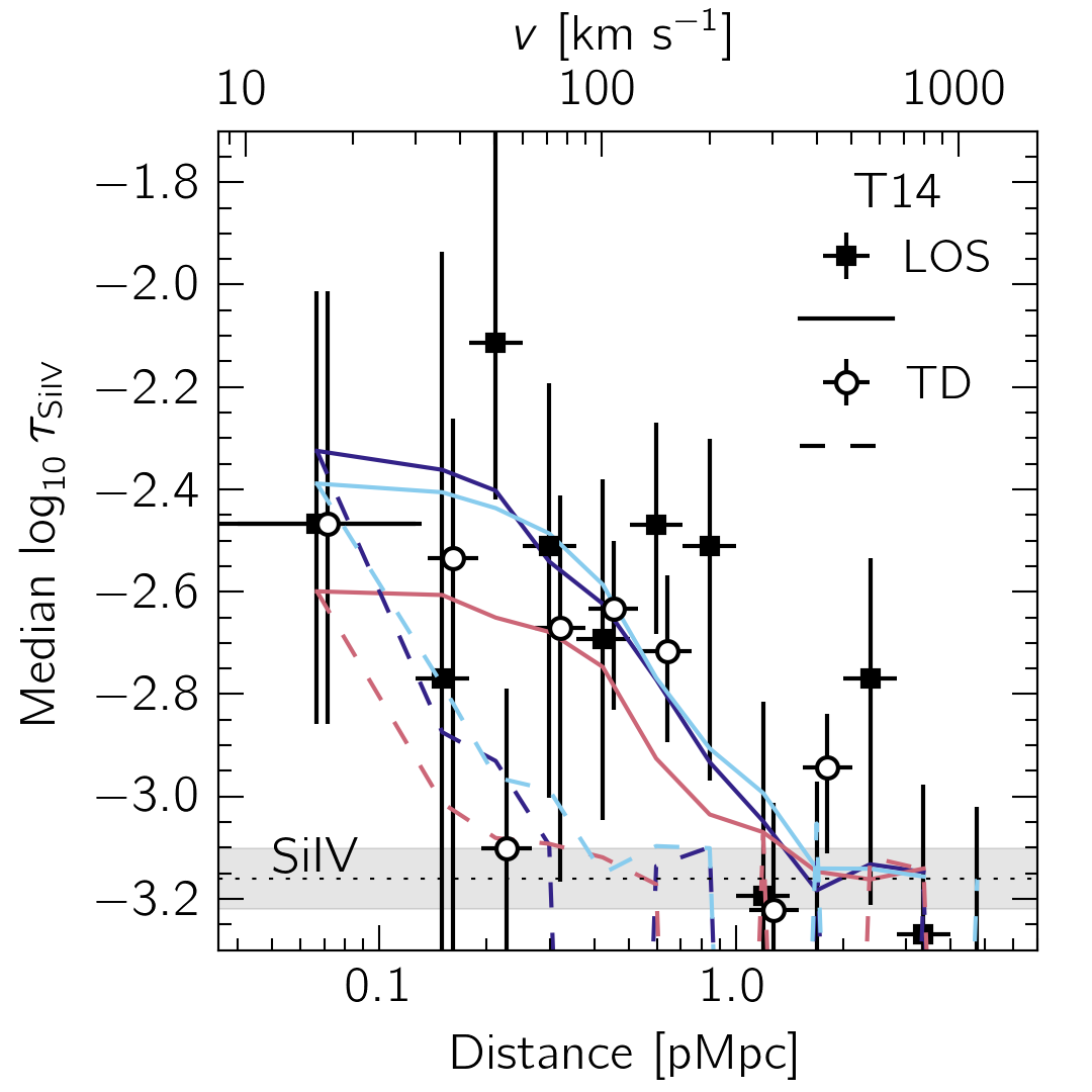
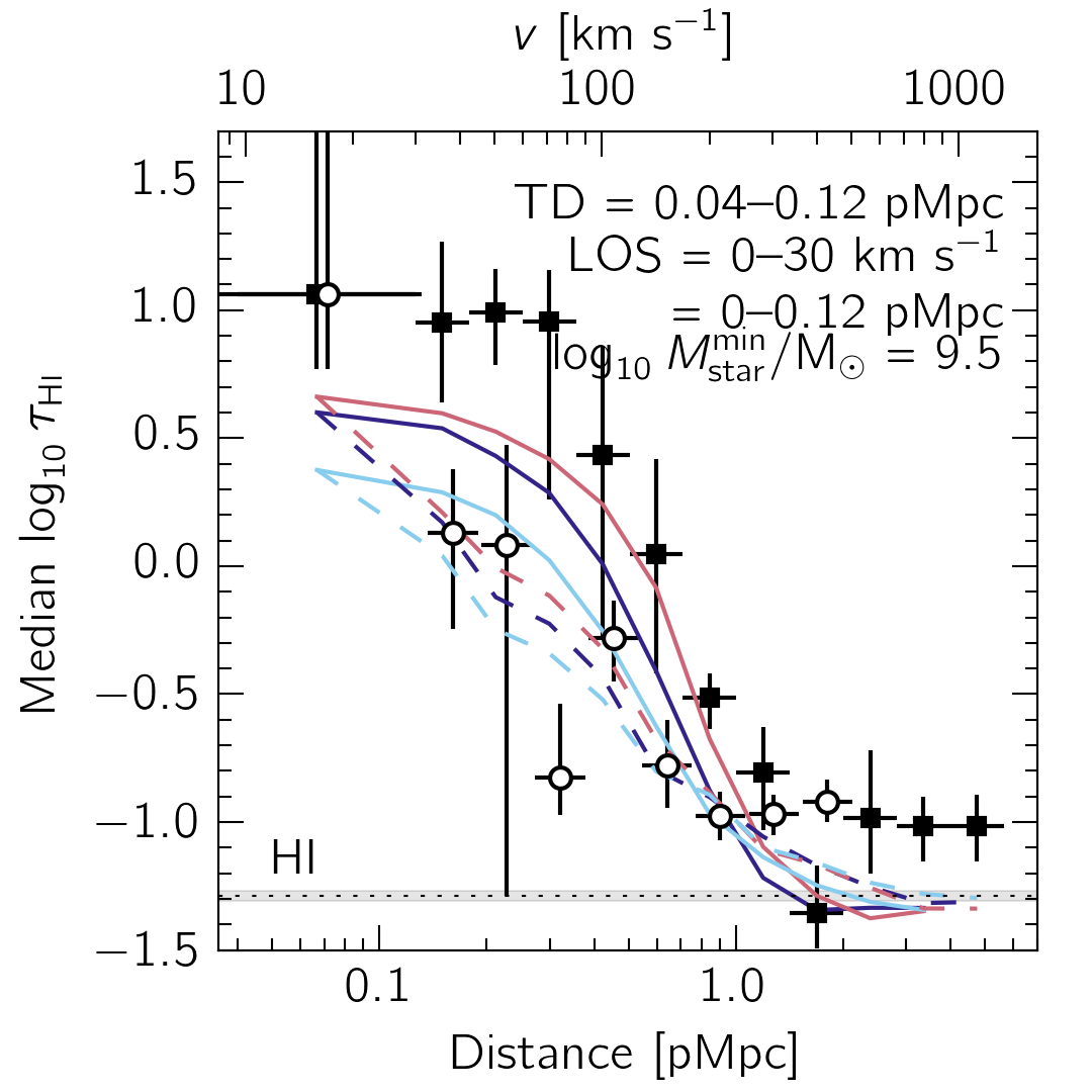
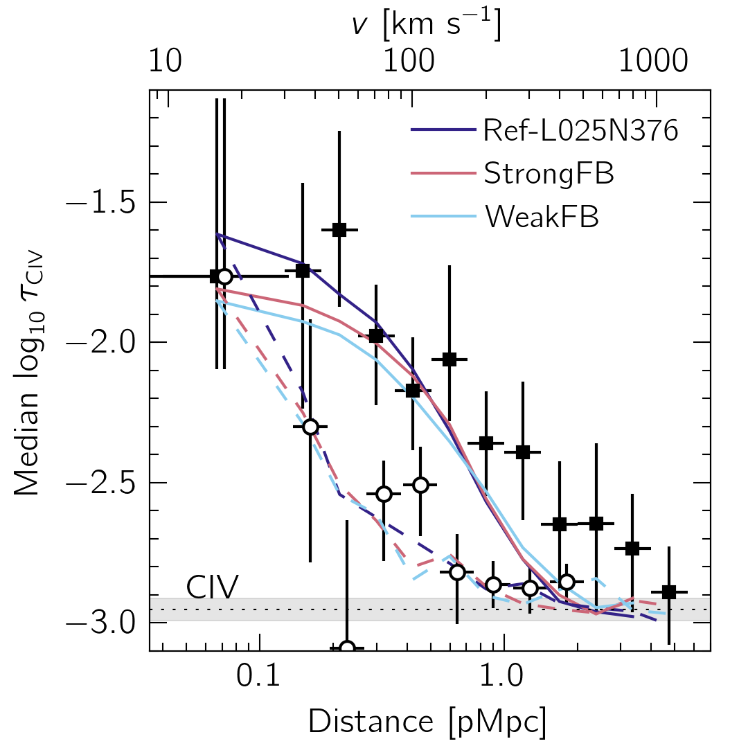
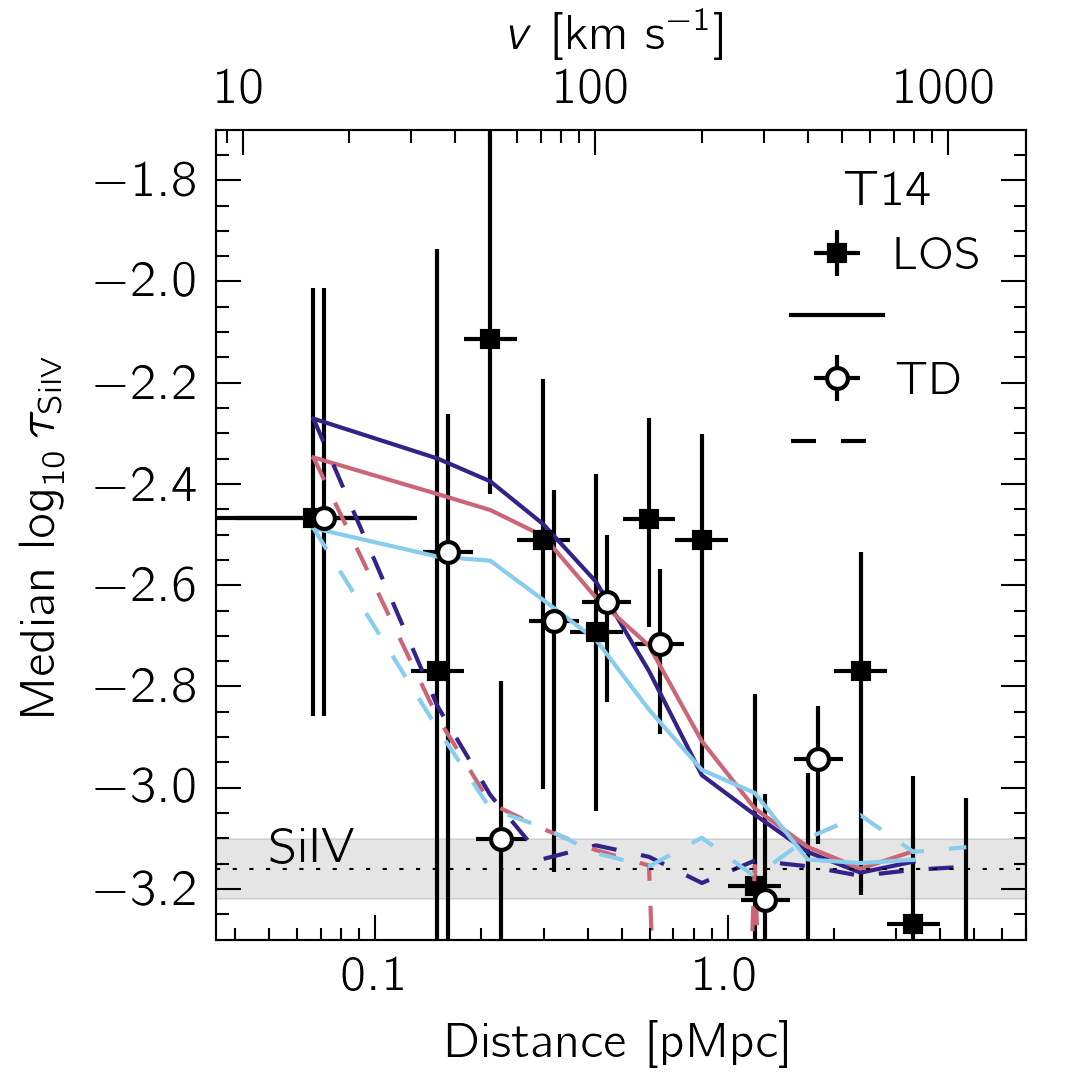
Figure 11: As Fig. 6, but for different EAGLE stellar subgrid prescriptions. In the top row we have used a fixed minimum halo mass of $M_{\rm halo}^{\rm min}=10^{11.5}$ M_⊙, while in the bottom row a fixed stellar mass of $M_{\ast}^{\rm min}=10^{9.5}$ M_⊙is considered. We show the reference model, as well as results from the WeakFB and StrongFB runs, all using a 25 cMpc box. At fixed halo mass, the metal-line absorption around our galaxies does not depend strongly on feedback models. This indicates that the observed redshift-space distortions are likely not dominated by outflows, but rather by infall or virial motions set by the mass of the halo.

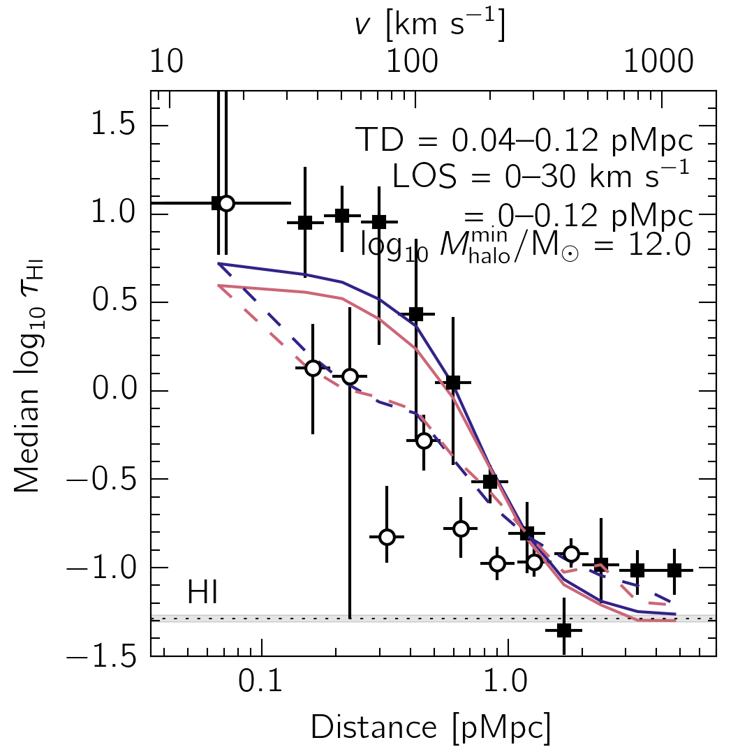
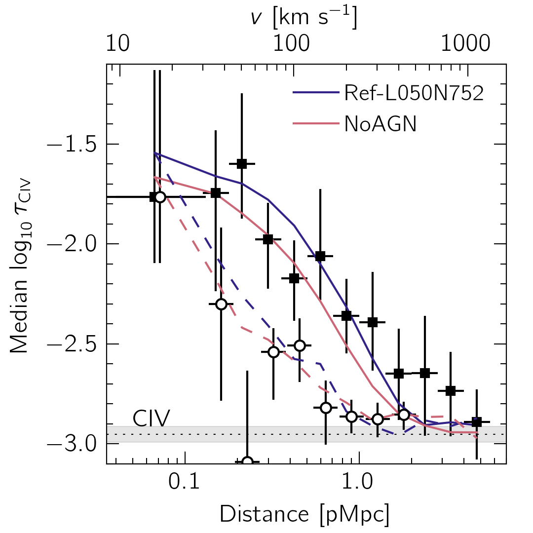
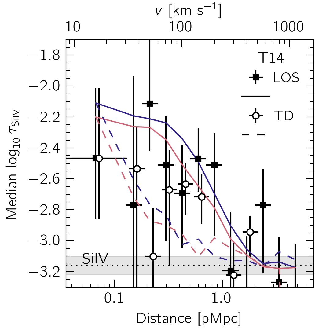
Figure 12: As Fig. 6, but for different AGN feedback prescriptions. We examine both the Ref and NoAGN models using a 50 cMpc box, and find that turning off AGN feedback does not have a significant impact on the optical depth profiles.

In § 4, we explored the effect that varying the stellar feedback models had on velocities of the gas particles, and found that the ion mass-weighted radial velocities depend on halo mass (rather than stellar mass) and are primarily infalling. In this section, we examine the impact that modifying the feedback model has on the metal-line optical depths, and interpret the findings in the context of the results from § 4.

Fig. 11 presents the outcome of varying the subgrid stellar feedback for both a fixed minimum halo mass (top row) and stellar mass (bottom row). We compare the median optical depths from Ref-L025N0376 to the WeakFB and StrongFB runs, which use respectively half and twice as efficient stellar feedback as the reference model. Note that because these models use a 25 cMpc box, so at large transverse distances the results will not be converged with the size of the simulation volume.

First examining the top row, we find that the optical depth profiles for Hi, Civ and Siiv do not depend strongly on the feedback model at fixed minimum halo mass. While there are small differences between the models, these differences are not larger than the errors on the data. This is consistent with the finding from § 4 that the ion mass-weighted gas velocities do not change with feedback model for fixed minimum halo mass, as the gas probed is mainly infalling and has a radial velocity set by halo mass. Furthermore, the results for Hi are in agreement with Rakic et al. (2013), who found that Hi optical depths around galaxies are set primarily by halo mass and are not strongly influenced by feedback model.

Next, in the bottom row of Fig. 11 we show the same optical depth profiles, but using a fixed minimum stellar mass of $10^{9.5}$ M_⊙. In the case of Hi, we see an expected variation of the optical depth with subgrid model, where Hi optical depths increase with feedback strength (or halo mass). On the other hand, for Civ and Siiv we find very little variation with halo mass. This may be due to two competing effects: halo mass and metallicty. Specifically, while we know the the infall velocities increase with halo mass (stronger feedback), we have also found that at fixed stellar mass, Civ- and Siiv-weighted metallicity is higher with decreasing halo mass (weaker feedback), and the two effects my be cancelling out.

Finally, in Fig. 12 we compare the median optical depths from the NoAGN run to the 50 cMpc reference model, Ref-L050N752. We presents results for $M_{\rm halo}^{\rm min}=10^{12.0}$ M_⊙, as we do not expect the exclusion of AGN to have a strong effect below this halo mass. Overall, we do not find that the presence of AGN feedback has a significant impact on the median optical depth profiles.

References

- Aguirre et al. (2002) Aguirre, A., Schaye, J., & Theuns, T. 2002, ApJ, 576, 1
- Bahé et al. (2016) Bahé, Y. M., Crain, R. A., Kauffmann, G., et al. 2016, MNRAS, 456, 1115
- Bielby et al. (2016) Bielby, R. M., Shanks, T., Crighton, N. H. M., et al. 2016, ArXiv e-prints, arXiv:1610.09144
- Booth & Schaye (2009) Booth, C. M., & Schaye, J. 2009, MNRAS, 398, 53
- Chabrier (2003) Chabrier, G. 2003, PASP, 115, 763
- Cowie & Songaila (1998) Cowie, L. L., & Songaila, A. 1998, Nature, 394, 44
- Crain et al. (2015) Crain, R. A., Schaye, J., Bower, R. G., et al. 2015, MNRAS, 450, 1937
- Crain et al. (2017) Crain, R. A., Bahé, Y. M., Lagos, C. d. P., et al. 2017, MNRAS, 464, 4204
- Dalla Vecchia & Schaye (2012) Dalla Vecchia, C., & Schaye, J. 2012, MNRAS, 426, 140
- Dolag et al. (2009) Dolag, K., Borgani, S., Murante, G., & Springel, V. 2009, MNRAS, 399, 497
- Durier & Dalla Vecchia (2012) Durier, F., & Dalla Vecchia, C. 2012, MNRAS, 419, 465
- Ellison et al. (2000) Ellison, S. L., Songaila, A., Schaye, J., & Pettini, M. 2000, AJ, 120, 1175
- Faucher-Giguère et al. (2016) Faucher-Giguère, C.-A., Feldmann, R., Quataert, E., et al. 2016, MNRAS, 461, L32
- Faucher-Giguère et al. (2015) Faucher-Giguère, C.-A., Hopkins, P. F., Kereš, D., et al. 2015, MNRAS, 449, 987
- Ford et al. (2016) Ford, A. B., Werk, J. K., Davé, R., et al. 2016, MNRAS, 459, 1745
- Fumagalli et al. (2014) Fumagalli, M., Hennawi, J. F., Prochaska, J. X., et al. 2014, ApJ, 780, 74
- Furlong et al. (2015a) Furlong, M., Bower, R. G., Theuns, T., et al. 2015a, MNRAS, 450, 4486
- Furlong et al. (2015b) Furlong, M., Bower, R. G., Crain, R. A., et al. 2015b, ArXiv e-prints, arXiv:1510.05645
- Haardt & Madau (2001) Haardt, F., & Madau, P. 2001, in Clusters of Galaxies and the High Redshift Universe Observed in X-rays, ed. D. M. Neumann & J. T. V. Tran
- Hopkins (2013) Hopkins, P. F. 2013, MNRAS, 428, 2840
- Hummels et al. (2013) Hummels, C. B., Bryan, G. L., Smith, B. D., & Turk, M. J. 2013, MNRAS, 430, 1548
- Kawata & Rauch (2007) Kawata, D., & Rauch, M. 2007, ApJ, 663, 38
- McAlpine et al. (2016) McAlpine, S., Helly, J. C., Schaller, M., et al. 2016, Astronomy and Computing, 15, 72
- Meiksin et al. (2017) Meiksin, A., Bolton, J. S., & Puchwein, E. 2017, MNRAS, arXiv:1701.06948
- Meiksin et al. (2015) Meiksin, A., Bolton, J. S., & Tittley, E. R. 2015, MNRAS, 453, 899
- Oppenheimer & Schaye (2013) Oppenheimer, B. D., & Schaye, J. 2013, MNRAS, 434, 1063
- Oppenheimer et al. (2016) Oppenheimer, B. D., Crain, R. A., Schaye, J., et al. 2016, MNRAS, 460, 2157
- Planck Collaboration et al. (2014) Planck Collaboration, Ade, P. A. R., Aghanim, N., et al. 2014, A&A, 571, A16
- Prochaska et al. (2011) Prochaska, J. X., Weiner, B., Chen, H.-W., Mulchaey, J., & Cooksey, K. 2011, ApJ, 740, 91
- Rahmati et al. (2015) Rahmati, A., Schaye, J., Bower, R. G., et al. 2015, MNRAS, 452, 2034
- Rahmati et al. (2016) Rahmati, A., Schaye, J., Crain, R. A., et al. 2016, MNRAS, 459, 310
- Rakic et al. (2013) Rakic, O., Schaye, J., Steidel, C. C., et al. 2013, MNRAS, 433, 3103
- Rakic et al. (2011) Rakic, O., Schaye, J., Steidel, C. C., & Rudie, G. C. 2011, MNRAS, 414, 3265
- Rakic et al. (2012) —. 2012, ApJ, 751, 94
- Rosas-Guevara et al. (2015) Rosas-Guevara, Y. M., Bower, R. G., Schaye, J., et al. 2015, MNRAS, 454, 1038
- Rudie et al. (2012) Rudie, G. C., Steidel, C. C., Trainor, R. F., et al. 2012, ApJ, 750, 67
- Schaller et al. (2015) Schaller, M., Dalla Vecchia, C., Schaye, J., et al. 2015, MNRAS, 454, 2277
- Schaye (2004) Schaye, J. 2004, ApJ, 609, 667
- Schaye et al. (2003) Schaye, J., Aguirre, A., Kim, T.-S., et al. 2003, ApJ, 596, 768
- Schaye & Dalla Vecchia (2008) Schaye, J., & Dalla Vecchia, C. 2008, MNRAS, 383, 1210
- Schaye et al. (2000) Schaye, J., Rauch, M., Sargent, W. L. W., & Kim, T.-S. 2000, ApJ, 541, L1
- Schaye et al. (2010) Schaye, J., Dalla Vecchia, C., Booth, C. M., et al. 2010, MNRAS, 402, 1536
- Schaye et al. (2015) Schaye, J., Crain, R. A., Bower, R. G., et al. 2015, MNRAS, 446, 521
- Segers et al. (2017) Segers, M. C., Oppenheimer, B. D., Schaye, J., & Richings, A. J. 2017, ArXiv e-prints, arXiv:1704.05470
- Shen et al. (2013) Shen, S., Madau, P., Guedes, J., et al. 2013, ApJ, 765, 89
- Springel (2005) Springel, V. 2005, MNRAS, 364, 1105
- Springel et al. (2005) Springel, V., Di Matteo, T., & Hernquist, L. 2005, MNRAS, 361, 776
- Springel et al. (2001) Springel, V., White, S. D. M., Tormen, G., & Kauffmann, G. 2001, MNRAS, 328, 726
- Steidel et al. (2010) Steidel, C. C., Erb, D. K., Shapley, A. E., et al. 2010, ApJ, 717, 289
- Steidel et al. (2014) Steidel, C. C., Rudie, G. C., Strom, A. L., et al. 2014, ApJ, 795, 165
- Stinson et al. (2012) Stinson, G. S., Brook, C., Prochaska, J. X., et al. 2012, MNRAS, 425, 1270
- Suresh et al. (2015a) Suresh, J., Bird, S., Vogelsberger, M., et al. 2015a, MNRAS, 448, 895
- Suresh et al. (2015b) Suresh, J., Rubin, K. H. R., Kannan, R., et al. 2015b, ArXiv e-prints, arXiv:1511.00687
- Theuns et al. (1998) Theuns, T., Leonard, A., Efstathiou, G., Pearce, F. R., & Thomas, P. A. 1998, MNRAS, 301, 478
- Trainor & Steidel (2012) Trainor, R. F., & Steidel, C. C. 2012, ApJ, 752, 39
- Trayford et al. (2015) Trayford, J. W., Theuns, T., Bower, R. G., et al. 2015, MNRAS, 452, 2879
- Tumlinson et al. (2011) Tumlinson, J., Thom, C., Werk, J. K., et al. 2011, Science, 334, 948
- Tummuangpak et al. (2014) Tummuangpak, P., Bielby, R. M., Shanks, T., et al. 2014, MNRAS, 442, 2094
- Turner et al. (2016) Turner, M. L., Schaye, J., Crain, R. A., Theuns, T., & Wendt, M. 2016, MNRAS, 462, 2440
- Turner et al. (2014) Turner, M. L., Schaye, J., Steidel, C. C., Rudie, G. C., & Strom, A. L. 2014, MNRAS, 445, 794
- Turner et al. (2015) —. 2015, MNRAS, 450, 2067
- Wiersma et al. (2009a) Wiersma, R. P. C., Schaye, J., & Smith, B. D. 2009a, MNRAS, 393, 99
- Wiersma et al. (2009b) Wiersma, R. P. C., Schaye, J., Theuns, T., Dalla Vecchia, C., & Tornatore, L. 2009b, MNRAS, 399, 574